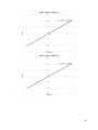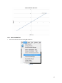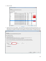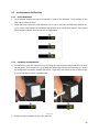
1
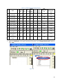
Lab Manual Contributors: Adam Mueller Bilal Ahamed Mohammed Hezha Lutfalla Sadraddinler Ahmad Sear Rahimi Mohammed Ismail Ahmed Xiaoyun Shao Version 2.3 12/02/2014 Western Michigan University’s Laboratory of Earthquake and Structural Simulation (LESS) is located at C113 in the College of Engineering and Applied Sciences (CEAS) building in Kalamazoo, Michigan. It is a state-of-the-art facility for simulating earthquakes and the effects on small scale structures. The major equipment in the LESS includes a uniaxial seismic simulator (commonly called a shake table), two 3 kips hydraulic actuators with the supporting hydraulic power supply and advanced real time controller. Instrumentation available in the lab consists of accelerometers, a linear variable displacement transducer (LVDT), and a wireless sensor network set. Through this equipment, various seismic experiments can be performed, including shake table test, effective force test, and pseudodynamic test in real time and with substructuring. Version 2.3: Improved Shake table testing procedure, added steps to load 10 ground motions with the ground motion information provided (Section 4.4). Added Section 4.5 Shake table motion generation using Seismosignal. Improved Section 5.3 Real-time Controller Formatting and Software Installation using NI Measurement and Automation Explorer (MAX). Specifically, steps on how to choose the Chassis in the MAX and the images of the real-time controller after important steps are provided. Improved Section 5.5 Hybrid Testing Procedure with the steps to input calibration equation of the structural actuator (1) external command; (2) LVDT and (3) Load cell in the workscope of the NI Veristand. Modified method of calibration structure LVDTs using MAX are provided in Section 6.4. Version 2.2: Added command calibration section (3.2.6) Version 2.1: Added instrumentation frame section (section 3.4.3) Updated substructure specimen information (section 3.5.2) Updated logging in hybrid testing procedure (section 5.5) Added section on UI-SimCor and NICON (section 5.6) Updated LVDT installation procedure (section 6.1) Added referenced single-ended (RSE) note to system explorer (section 6.4) 1 Version 2.0: Added actuator tuning procedure (section 3.2.5) Updated hybrid testing procedure (section 5.5) o More information on system mappings o Revised primary control loop rate step o More information on deployment procedure o More information on graph setup o Added instrumentation offset procedure 2 Table of Contents 1 Overview ............................................................................................................................................... 6 2 Test Methods in Earthquake Engineering ............................................................................................. 7 3 2.1 Quasi-Static Testing ...................................................................................................................... 7 2.2 Shake Table Testing ...................................................................................................................... 7 2.3 Effective Force Testing .................................................................................................................. 7 2.4 Pseudodynamic Testing ................................................................................................................ 7 2.5 Real Time Dynamic Hybrid Testing ............................................................................................... 8 Equipment ............................................................................................................................................. 9 3.1 3.1.1 Base Frame ............................................................................................................................ 9 3.1.2 Sliding Table .......................................................................................................................... 9 3.1.3 Capacity ................................................................................................................................. 9 3.2 Hydraulic System......................................................................................................................... 10 3.2.1 Hydraulic Power Supply ...................................................................................................... 10 3.2.2 Hydraulic Controller SC6000 ............................................................................................... 10 3.2.3 Hydraulic Linear Actuators .................................................................................................. 11 3.2.4 Hydraulic System Maintenance .......................................................................................... 11 3.2.5 Actuator Tuning Procedure ................................................................................................. 12 3.2.6 Command Calibration ......................................................................................................... 18 3.3 NI-Controller and Data Acquisition ............................................................................................. 19 3.4 Instrumentation .......................................................................................................................... 19 3.4.1 Accelerometers ................................................................................................................... 19 3.4.2 LVDT .................................................................................................................................... 21 3.4.3 Instrumentation Frame ....................................................................................................... 21 3.5 4 Uniaxial Shake Table ..................................................................................................................... 9 Specimens ................................................................................................................................... 21 3.5.1 Structure Specimen ............................................................................................................. 21 3.5.2 Substructure Specimen ....................................................................................................... 22 Open Loop Testing Procedure ............................................................................................................ 25 4.1 Hydraulic Equipment Startup Procedure .................................................................................... 25 4.2 Hydraulic shut-down procedure ................................................................................................. 28 4.3 Cyclic Testing ............................................................................................................................... 29 3 5 4.4 Shake Table Testing with Earthquake Record............................................................................. 33 4.5 Shake table motion generation using SeismoSignal ................................................................... 38 Hybrid Testing Controller Systems and Operation ............................................................................. 43 5.1 Hardware Integration.................................................................................................................. 43 5.1.1 Internal Hydraulic Control Connection ............................................................................... 43 5.1.2 General DAQ Connection .................................................................................................... 43 5.1.3 External Hybrid Testing Connection.................................................................................... 43 5.2 Software Integration ................................................................................................................... 45 5.3 Real-time Controller (RTC) Formatting and Software Installation using NI Measurement and Automation Explorer (MAX).................................................................................................................... 46 5.4 Creating System Definition File in NI-VeriStand ......................................................................... 52 5.5 Hybrid Testing Procedure ........................................................................................................... 54 5.5.1 BUILD MODEL ...................................................................................................................... 54 5.5.2 DEPLOY MODEL ................................................................................................................... 55 5.5.3 SETUP WORKSPACE............................................................................................................. 59 5.5.4 Input Calibration Equation .................................................................................................. 61 5.5.5 ENABLE EXTERNAL CONTROL .............................................................................................. 62 5.5.6 OFFSET INSTRUMENTATION ............................................................................................... 63 5.5.7 RECORD DATA ..................................................................................................................... 67 5.5.8 RUN TEST............................................................................................................................. 69 5.5.9 DISABLE EXTERNAL CONTROL ............................................................................................. 70 5.5.10 VIEW DATA .......................................................................................................................... 70 5.6 6 Hybrid Testing with UI-SimCor and NICON ................................................................................. 70 5.6.1 UI-SimCor Configuration ..................................................................................................... 70 5.6.2 NICON Configuration........................................................................................................... 71 5.6.3 Procedure ............................................................................................................................ 73 5.6.4 Geographically Distributed Procedure................................................................................ 77 Instrumentation .................................................................................................................................. 79 6.1 LVDT Installation ......................................................................................................................... 79 6.2 Accelerometer Installation.......................................................................................................... 81 6.3 Adding Instrumentation in System Explorer ............................................................................... 82 6.4 LVDT Calibration.......................................................................................................................... 83 4 6.4.1 Operation in the Measurement & Automation Explorer (MAX)......................................... 83 6.4.2 Setting up the sLVDTs for calibration.................................................................................. 84 6.4.3 sLVDT calibration ................................................................................................................ 85 6.4.4 APPLY CALIBRATION ............................................................................................................ 87 6.5 Accelerometer Calibration .......................................................................................................... 89 7 Contact Information............................................................................................................................ 90 8 Appendix 1: Data Acquisition Channels of SCB-68.............................................................................. 91 9 8.1 PXI1Slot2 ..................................................................................................................................... 92 8.2 PXI1Slot8 ..................................................................................................................................... 92 Appendix II: Calibration Equations of all the instruments .................................................................. 93 5 1 Overview Western Michigan University’s Laboratory of Earthquake and Structural Simulation (LESS) is located at C113 in the College of Engineering and Applied Sciences (CEAS) building in Kalamazoo, Michigan. It is a state-of-the-art facility for simulating earthquakes and the effects on small scale structures. The major equipment in the LESS includes a uniaxial seismic simulator (commonly called a shake table), two 3 kips hydraulic actuators with the supporting hydraulic power supply and advanced real time controller. The shake table has a dimension of 3 ft x 3 ft and can subject a specimen with maximum weight of 500 lb to an earthquake time history with peak acceleration up to 4g. Structural dynamic properties and structural response due to seismic attack can be obtained through such a shake table test. Instrumentation available in the lab consists of accelerometers, a linear variable displacement transducer (LVDT), and a wireless sensor network set. Through this equipment, various seismic experiments can be performed, including shake table test, effective force test, and pseudodynamic test in real time and with substructuring. Firstly, several common test methods in earthquake engineering are presented. Next, the LESS equipment is introduced. The function of each component is briefly described followed by basic specifications. Subsequently, open loop testing as well as hybrid testing is explained with specific pictorial instructions. 6 2 Test Methods in Earthquake Engineering There are several common testing methods including quasi-static loading testing (QST), shake table testing (STT), effective force testing (EFT), pseudodynamic (PSD) testing, and real time dynamic hybrid testing (RTDHT). When these experiments are conducted only on the physical substructure and combined with numerical simulation of the remaining numerical substructure, they are defined as hybrid testing, during which the seismic response of the entire system is obtained. 2.1 Quasi-Static Testing The QST method involves slowly applying predefined cyclic displacement or force history to a test structure using hydraulic actuators. QST is generally used for single structural elements or simple subassemblages to obtain their hysteretic responses that can be used to predict the seismic performance in some cases. However QST does not capture the specimen inertia effects that are associated with the dynamic nature of seismic loadings. 2.2 Shake Table Testing The STT is a dynamic testing method during which a structural specimen is mounted on a shake table that will simulate an earthquake ground motion. The effect of inertia force on the structure is naturally developed and can be directly observed and measured. STT allows realistic representation of earthquake effects on the structure under investigation; however, the size of the structure being tested is limited to the size of the shake table. It can be difficult for a small scale specimen to accurately represent a complex full size structural system. In addition to scaling, shake table requires an advanced control system that can reduce actuator lag and compensate for the reaction forces between the structural specimen and the table, which is usually expensive and requires further research to improve. 2.3 Effective Force Testing During EFT the base of a structure is fixed to a strong floor. Dynamic force is applied to the structure representing the real inertia force the structure will experience during an earthquake. This dynamic force is the product of the acceleration of the selected ground motion and the structural mass, and is usually applied utilizing an actuator/reaction loading system. This method removes the dependency on a shake table and allows a full scale structure to be tested. However, the reliability of EFT is highly dependent on the accuracy of the force control in the actuators. Since force measurements are usually sensitive to the noise, actuator force control remains to be a challenge which needs to be conquered to further advance EFT. 2.4 Pseudodynamic Testing PSD test is a hybrid test in essence since it uses numerical simulation during the physical experiment to study the structural dynamic behavior subject to seismic attack. The test structure is usually loaded quasistatically with the simulated displacement response obtained from a computer model, while the corresponding resisting force is fed back to the model to calculate the next step’s displacement command. The real time PSD test was developed to exam the dynamic response of velocity-dependent devices which cannot be accurately captured during quasi-static loading. The advantage of PSD testing is that it allows experimentation on any size of structures, as compared to the general STT that is limited to be performed 7 on reduced size structures. Therefore, PSD testing has been used in numerous earthquake engineering research projects. However, the real time testing still poses a challenge to this method especially when a large scale complex specimen is being tested. 2.5 Real Time Dynamic Hybrid Testing The real time dynamic hybrid testing (RTDHT) method was proposed as a seismic response simulation method that combines numerical computation and physical specimens excited by both shake tables and auxiliary actuators. The loadings generated by the seismic excitations at the interfaces between the physical and numerical substructures, in terms of accelerations and forces, are imposed by shake tables and actuators in a step-by-step manner at a real time rate. The unique aspect of the RTDHT method is the versatile implementation of inertia forces and a force based substructuring. However RTDHT has not been adopted by a research project as a testing method due to some difficulties in numerical simulation and coordinated real time control of both actuators and shake tables. Therefore, more research is necessary to implement this advanced versatile testing method in real research projects. 8 3 Equipment 3.1 Uniaxial Shake Table 3.1.1 Base Frame The dimensions of the base frame are 8 ft x 3 ft x 4 in. Its weight is 1400 lb. The base frame exists solely for the purpose of supporting the shake table and reaction frame. Figure 3-1: Base Frame and Sliding Table 3.1.2 Sliding Table The uniaxial shake table is designed to impose base ground motion to a test specimen. It does this by moving along two 36 in steel guide rails. It can be utilized alone in a shake table test or shake table substructure test, or it can be combined with the actuator/reaction frame to conduct a real time dynamic hybrid test. When only the actuator/reaction frame is used in a hybrid test, the shake table can be used as a strong floor to hold the test specimen with the 2 in (5.08 cm) space bolt hole pattern for easy and flexible installation. Table 3-1: Sliding Table Specifications Dimensions Weight Maximum specimen mass Frequency of operation Maximum specimen acceleration Displacement 3.1.3 3 ft x 3 ft x 2 in aluminum plate 310 lb 500 lb (228 kg) 0 - 20 Hz 4 g (with 500 lb specimen) ± 3 in Capacity Table 3-2: Capacities of Materials used in Shake Table Material Tensile Yield Strength (ksi) Ultimate Tensile Strength (ksi) 37 42 ASTM A500 Grade B Steel • Base Frame • Reaction Frame 45.7 58 A36 Steel • Base Plates 36.3 58 Aluminum 6061-T6 • Sliding Table • End Support Blocks • Pillow Blocks 9 3.2 Hydraulic System 3.2.1 Hydraulic Power Supply The hydraulic power supply (HPS) used in the testing system is a Servo Quality 10 gpm Model No. 110.11S. It sends hydraulic fluid to both actuators with a 20 horsepower electric motor to pump up to 10 gpm at 3000 psi. The hydraulic oil passes through a 3 micron high pressure filter. The HPS contains control buttons to switch between high and low pressure as well as an on/off button. It also has an emergency stop button which allows the immediate shut down of the pump and keeps the pump from turning on until the problem is corrected. Figure 3-2: Hydraulic Power Supply 3.2.2 Hydraulic Controller SC6000 The manufacturer’s generic hydraulic controller adopted herein is a 2 channel (one for each actuator) desk top controller called Shore Western SC6000. It uses Windows XP operating system and commands the entire hydraulic system including the on/off switch, the pressure of the HPS, and the two actuators’ motions. The controller connects the hydraulic system via input/output connectors which are attached to the load cells, LVDTs, servo-valves, service manifolds, and the HPS. It uses a proportional–integral– derivative controller for displacement control of the actuators. Having a user graphical interface the controller can be easily operated to adjust control parameters, run tests, record feedback, and tune the system to reach its optimum performance. See the SC6000 Manual for detailed operation instructions. The hydraulic controller is also capable of tracking external command for real time operation. This feature is essential for this system to conduct hybrid testing. External command of the actuators (i.e. simulated interface motion between the physical and numerical substructures determined from the numerical simulation running in a real-time controller) can therefore be transferred to the hydraulic controller to drive the actuators applying the desired dynamic loading to the structural specimen. 10 Figure 3-3: Hydraulic Controller SC6000 3.2.3 Hydraulic Linear Actuators The hybrid testing system includes two hydraulic linear actuators (Shore Western Model 910D-1.08-6(0)4-1348). Each actuator contains a 2.5 gpm servo-valve and a hydraulic service manifold rated at 15 gpm. The actuators are installed with linear variable differential transducers (LVDT) and load cell sensors, which provide position and loading feedback for both displacement and force control of the actuators. One actuator is used to drive the shake table and is named the table actuator. The other actuator is mounted against the reaction frame to form an actuator/reaction setup and is called the structure actuator. The hybrid testing system developed therefore consists of both shake table and actuator/reaction setup allowing hybrid tests to be conducted using individual loading equipment or both of them simultaneously. This loading capability along with numerical simulation, results in various testing configurations necessary to perform different hybrid testing methods. Table 3-3: Actuator Specifications Force Stroke Swivel Base and End Rod Servo-valve Load Cell Hydraulic Service Manifolds ± 3240 lb at 3000 psi 6 inch, ± 2.5 inch, plus ± 0.5 inch cushions ± 90° swivel, ± 7° tilt 2.5 gpm at 1000 psi 2.5 kip fatigue rated 300% overload capacity 15 gpm at 3000 psi oil service Figure 3-4: Actuators 3.2.4 Hydraulic System Maintenance Always warm up the HPS before performing a dynamic type test. The controller also needs to warm up for calibration (for about 2 hours running). For safety, put the green cable (ground cable) under the LVDT connection or servo valve or ground base plate. 11 When actuators are not being used or are being stored for a relatively long time, fully retract the stroke to avoid dust. If dust is visible on the actuators, wipe it off. Clean oil, clean oil, and clean oil!!! Never open to atmosphere and always put the caps on. Loose cable of the instrument for possible movement of the actuators. Straighten hoses while running HPS. Never step on hoses. Do not put hoses across sharp edge. Check hose once a month for rubber break. Retract stroke of both actuators after each operation. This will prevent dust resting on the stroke and contamination of the oil. No oil on the floor. Never plug/unplug cables when HPS is running. Always make a copy of the folder C:/Programs/ShoreWesternMfg/swcs/. Play with software/setting using copies instead of original one. Change filters every 6 months or 1000 hours of use. First time change shall be around a couple hundred hours of running HPS. Regularly check hoses and connections for leakage. If a leakage is detected: 1) Tighten the fittings, 2) Change fittings, GIC standard off the shelf product. For calibration, follow ASTM E09. Calibrate once a year. 3.2.5 Actuator Tuning Procedure 1. Startup the hydraulic equipment (see Section 4.1). 2. Type 0 into the table actuator displacement command in SC6000. Press enter. If the position is not exactly 0 inches, the valve balance must be adjusted. Figure 3-5 3. To adjust the valve balance, first click the blue triangle in the Valve Driver 1 box in the lower right panel. Figure 3-6 12 4. Now click Valve Balance. Figure 3-7 5. Adjust the slider until the position reading is 0 inches. Figure 3-8 Figure 3-9 6. Right click Waveform in the upper left panel of the screen. Click Change selected cards. Click Card 1, click ADD, and then click OK. Figure 3-10 13 7. In the upper left panel, right click Card 1 and select table actuator. Figure 3-11 8. Right click actuator and click Add Segment. Then click Square Wave. Figure 3-12 9. Use an amplitude of 0.25 inches, a duty cycle of 50%, a frequency of 0.2 Hz, and a large number of cycles. Click OK. Figure 3-13 10. Click the blue triangle in the Servo Amplifier 1 box in the lower right panel. Figure 3-14 14 11. Click Monitor A next to the Internal Command box. Also click the Proportional gain and the Rate gain. The sliders shown below will appear. There is no need to adjust the Integrator gain, so do not click on it. Figure 3-15 Figure 3-16 Figure 3-17 12. Click Select Channels in the upper right panel of the screen and click OK on the dialogue box that appears. The channel colors should change. Make sure only the boxes next to MON A and TABLE POSITION are checked. 15 Figure 3-18 Figure 3-19 13. Click Run in the upper left panel and Start in the upper right panel. Adjust the y-axis and x-axis ranges so that the entire signals can be seen in the plot. Figure 3-20 Figure 3-21 16 14. The plot consists of two signals: the command being sent to the actuator and the actual displacement of the actuator recorded by the LVDT. The objective is to get these to match. 15. Adjusting the proportional gain will have the greatest effect and is the most important. If the actuator is too slow to reach its command displacement, the proportional gain must be increased. If the actuator is overshooting the command, causing vibrations, the proportional gain must be decreased. 16. The rate gain can also be adjusted, but will have less of an effect. Once again, the integrator gain does not need to be adjusted at all. The same steps can be followed to tune the structure actuator. EXAMPLES If the plot looks like this, the proportional gain is too low and needs to be increased. Figure 3-22 If the plot looks like this, the proportional gain is too high and needs to be decreased. 17 Figure 3-23 The following plot depicts a well-tuned actuator. Figure 3-24 3.2.6 Command Calibration The command calibration equations of both actuators may need to be updated periodically. If the LVDT readings are not matching with the displacement commands, performing command calibration will correct this. The command calibration procedure can be found in the SC6000 Software Operating Guide on pages 75-84. 18 3.3 NI-Controller and Data Acquisition The real-time controller consists of a real-time processor and the general purpose data acquisition (DAQ) cards. Both processor and DAQ cards are contained within a single chassis enabling real time data transfer between these two components without any delay. The real-time controller adopted herein is a National Instruments (NI) PXI system that has two DAQ cards, possessing a total of 48 analog input channels, 6 analog output channels, and 72 digital input/output channels. These channels receive the signals from the instrumentations that are attached to the test specimen and send external command to the hydraulic controller through the connections devised. The real-time processor processes the signal being sent and received through the DAQ cards and runs the hybrid testing model developed specifically for each test. Table 3-4: NI-Controller Specifications PXI 1050 Chassis 8-slot 3U PXI Chassis Integrated SCXI Chassis: 4 Signal Conditioning Module Slots PXI 8108 Controller 2.53 GHz Dual Core Embedded Controller PXI Modules PXI-6229: 16-bit, 32 AI, 48 DIO, Multifunction M Series DAQ PXI-6221: 16-bit, 16 AI, 24 DIO, Multifunction M Series DAQ SCB-68 68-pin Shielded Desktop Connector Block All communication to the DAQs travels through connector blocks Figure 3-25: NI-Controller 3.4 Instrumentation For general earthquake experiments, sensors are crucial to understand the performance of the test specimen under investigation. For hybrid testing, the data fed back from the sensors serve a double purpose. In addition to providing the specimen’s seismic response, some of the feedback data is also used to determine the interface loading and to improve the hydraulic loading performance. The sensors currently available for use include accelerometers and LVDTs. 3.4.1 Accelerometers Table 3-5: Wired Accelerometer Specifications 19 Wired Accelerometers (Crossbow Technology CXL04GP3) Input Range ± 4g Measurement 3 axis (x,y,z) Size 0.95" x 2" x 1.2" Weight 1.62 oz Figure 3-26: Wired Accelerometer Table 3-6: Wireless Accelerometer Specifications Wireless Accelerometer Network Set IIB2400 Interface Board Size 1.9" x 1.4" x 0.6" IPR2400 Intel Mote 2 (Imote 2) processor/radio board with external antennae Size 1.4" x 1.9" x 0.35" Structural Health Monitoring Accelerometer (SHM-A) sensor board IBB2400CA battery board with on/off switch Input Range ± 2g Measurement 3 axis (x,y,z) Figure 3-27: Wireless Accelerometer 20 3.4.2 LVDT Table 3-7: LVDT Specifications Input Voltage Stroke Frequency Response Power Supply Converter ± 15 V DC ± 5 in 200 Hz 115 V AC or 230 V AC Figure 3-28: LVDT 3.4.3 Instrumentation Frame The instrumentation frame is a 4’3” tall braced frame with three slots corresponding to story heights of the structure specimen. This allows for adjustment of instrumentation height. Figure 3-29: Instrumentation Frame 3.5 Specimens 3.5.1 Structure Specimen The structure specimen is an idealized lumped mass three degree-of-freedom (DOF) structure. Each story contains a mass which is supported by four columns. The columns are removable and replaceable, allowing for the separation of substructures while using the same materials of the full three story structure 21 test. The test specimen is very lightly damped (about 0.5% damping ratio). Therefore, an external damper is available that can be added to the top story to increase the structural damping to a realistic damping level of general civil structural systems. Number of Stories Story Height Structure Height Column Cross Section Story Weight Structure Weight Story Stiffness Natural Frequencies 3 12" 41 1/2" 1/8" x 1 1/4" 12.6 lb 37.7 lb 0.164 kip/in 5.04 Hz, 14.10 Hz, 20.30 Hz Table 3-8: Structure Specimen Specifications Figure 3-30: Structure Specimen 3.5.2 Substructure Specimen The substructure specimen is a cantilever column with an idealized plastic hinge connection at its base. The plastic hinge emulates nonlinear behavior and can be easily replaced after yielding without permanent damage to the specimen. The HSS 3” x 1.5” x 1/8” column is three feet long and is welded all around the base to a 5” x 12” steel plate with a ½” thickness. Two A307 steel bolts that are 4½” long and ¼” in diameter act as coupons on each side. These bolts have a center to center distance of 8”. They are each secured by two nuts that are fastened to the bottom of the upper plate and the top of the lower plate, which is 15” x 15” x ¾”. This lower plate is bolted in the four corners to the shake table in order to provide a fixed support. Two bearings are attached to 5” x 1¾” x ¾” aluminum plates, which are welded 22 to the bottom plate. The two bearings are 4” apart center to center. Finally, a 6” steel rod with a diameter of ½” connects the two new bearings to the hinge. Figure 3-31: Substructure Specimen Connection Figure 3-32: Substructure Specimen 23 2000 1500 Force (N) 1000 500 0 -500 -1000 -1500 -2000 -10 -5 0 5 Displacement (mm) 10 Figure 3-33: Typical Hysteretic Response of Substructure Specimen 24 4 Open Loop Testing Procedure During an open loop test, a predetermined loading pattern is imposed. Open loop testing does not require force responses to be measured in order to calculate displacement commands. Therefore, no feedback is needed and only a command signal is required. Open loop testing does not involve the use of the realtime controller and is only useful for certain types of tests, such as cyclic testing and shake table testing (STT), which are described in 4.2 and 4.3 respectively. 4.1 Hydraulic Equipment Startup Procedure 1. Make sure the water is turned on with both yellow levers in the up position (If you don’t, the hydraulics could overheat). Figure 4-1 2. If it’s not already on, turn on the computer (push both switches). Figure 4-2 25 If the controller is shut down previously due to an emergency stop such as the “Emergency” button shown below is pushed down, you need to first reset the “Emergency” follow the instruction shown below. 3. Double click the Shore Western start-up icon. Figure 4-3 4. In the lower left panel of the control screen, click the E-STOP RESET button (switching from DISABLED to ENABLED). Figure 4-4 26 5. On the front of the computer (black box) push the lighted red button (not the emergency stop button). Figure 4-5 6. In the lower left panel of the control screen, click the AUTOBALANCE button, then click the button labeled LOW under PUMP CONTROL. This will turn on the pump. Figure 4-6 7. Check hoses and fixtures for leaks. 8. To turn on the actuator, click the button labeled DISABLED for the appropriate actuator (this switches it to ENABLED). 27 Figure 4-7 9. To turn on high pressure, click the button labeled HIGH. Figure 4-8 10. To control the actuator, you can either use the slider in the lower left panel, enter the distance into the box next to the slider, or create a waveform in the upper left panel. 4.2 Hydraulic shut-down procedure When the test is done, fully retract actuator when there’s no specimen attached limiting actuator being fully retracted. This is beneficial to actuator when its stroke is not exposed to dust when not being utilized. To shut down the hydraulic, one may basically follow the inverse steps as done for the startup procedure, which is summarized below: Disable the actuator being used Click “low” to low pressure Click 28 4.3 Cyclic Testing A cyclic test can be performed using a sine wave sweep, but it is preferable to use a triangle wave increasing in amplitude over time. SC6000 has a built-in sine sweep, but does not have a built-in triangle wave. Therefore, a triangle wave must be created. This can be done in Microsoft Excel. When finished, save it as a .txt file. 4.3.1 ASSIGN LOAD 1. Right click Waveform in the upper left panel of the screen. Click Change selected cards. Click Card 1, click ADD, and then click OK. Figure 4-9 2. In the upper left panel, right click Card 1 and select structure actuator. Figure 4-10 3. Right click actuator and click Add Segment. Figure 4-11 4. Click Arbitrary Wave, click Load, select the waveform you created in Excel, and then click OK. 29 Figure 4-12 5. Setup necessary plots. In a scope plot, the x-axis is time. In an x vs. y plot, both axes are customizable. Figure 4-13 4.3.2 SETUP DATA LOGGING AND RUN TEST 1. Click Setup DAS and choose a name for your data file. Figure 4-14 2. Click Start DAS and Enable Logging. 30 Figure 4-15 3. Click Run in the upper left panel. Figure 4-16 4.3.3 PLOT DATA 1. After the test is complete, open MATLAB and click the Import Data button under the Workspace panel. The .txt data file will be in the SC6000_DATA folder on the Desktop. Figure 4-17 2. The Import Wizard will appear. Use 12 lines for the header and click Next. 31 Figure 4-18 3. In the next window, check “data” only. Click Finish. Figure 4-19 4. Type in the following commands into the command window in order to convert the data from metric units to English units and plot the data. Figure 4-20 32 5. The slope of the linear section on the plot is the stiffness (k) of the specimen. Figure 4-21 4.4 Shake Table Testing with Earthquake Record NOTE: The earthquake data must be saved in two columns, where the first column is time, and the second is displacement commands. The data has to be only in .txt file format, which can be created using Excel spreadsheet. The Units must only be in SI system as the SC6000 reads only SI units. Units are seconds for Time and meters for Displacement. Location of the EQ data files on SC6000 controller PC: All the EQ .txt files are saved under a folder by name EQ data which can be reached by the following link C:\Program Files\Shore Western Mfg\SWCS\WAVEFORMS\EQ\EQ data 33 No 1 2 3 4 5 6 7 8 9 1 0 Name NORTHR/MUL009 (Northridge) NORTHR/MUL279 (Northridge) NORTHR/LOS000 (Northridge) NORTHR/LOS270 (Northridge) DUZCE/BOL000 (Duzce, Turkey) DUZCE/BOL090 (Duzce, Turkey) HECTOR/HEC000 (Hector Mine) HECTOR/HEC090 (Hector Mine) IMPVALL/HDLT262 (Imperial Valley) IMPVALL/HDLT352 (Imperial Valley) Table 4-1 Available earthquake motions summary Time of Max. Max. Time of Magnit Scale Max. Max. Displacement EQ Velocity Max. ude Factor Acce. (g) Acce. (in) (in/sec) Vel.(sec) (sec) Time of Max. Displacement (sec) A1 6.7 0.57 0.28 8.04 13.23 8.77 2.95 8.45 A2 6.7 0.68 0.35 4.52 16.81 8.96 2.96 9.23 B1 6.7 0.65 0.27 4.67 11.01 6.38 3.00 4.68 B2 6.7 0.60 0.29 5.02 10.66 4.94 2.95 7.90 C1 7.1 0.33 0.24 10.75 7.34 11.25 3.00 15.96 C2 7.1 0.56 0.46 10.79 13.69 11.08 2.99 11.28 D1 7.1 0.33 0.09 5.98 3.71 11.28 2.93 9.41 D2 7.1 0.54 0.18 8.42 8.88 6.10 2.97 6.46 E1 6.5 0.63 0.15 8.80 6.45 54.22 2.97 54.82 E2 6.5 0.39 0.14 9.21 5.07 30.03 2.99 69.90 1. Right click “Waveform” in the upper left panel of the screen. Click “Change selected cards” and then click “Card” Figure 4-22 34 2. Click “ADD” and select “Card1”, then click “OK”. Figure 4-23 3. Card 1 will be added under the wave form in the upper left corner. Right click “Card 1” and select table actuator. Figure 4-24 4. Actuator will be added under the card 1. Right click actuator and click “Add Segment”. Figure 4-25 35 5. Select “Arbitrary Wave” to open the arbitrary wave load window a. Click “Load” to open the folder that contains the earthquake data files. If not, choose the folder through explorer as indicated in the beginning of this section. Figure 4-26 6. Select the earthquake (c1.txt as shown below as an example) and click “open” the earthquake will be loaded as shown in the “Arbitrary Wave” window. Click “OK” Figure 4-27 36 7. Show in the scope the selected earthquake input history. Select “X Vs Y” plot. Customize the x-axis as time and y-axis as the displacement history of the earthquake. The earthquake input history is now shown in the scope. Figure 4-28 Figure 4-29 8. In order to log and/or plot data, follow the same steps in section 4.2 “Cyclic Testing”. 37 4.5 Shake table motion generation using SeismoSignal SeismoSignal is one of the Seismosoft’s software which processes strong-motion data. It is a simple yet efficient software that performs the derivation of elastic and constant ductility inelastic response spectra, calculation of Fourier amplitude spectra, filtering and scaling high and low frequency records, and expecting other seismological parameters such as the Arian intensity and significant and effective duration. SeismoSignal can be downloaded easily from www.seismosoft.com and it is free for academic purposes. Researchers can obtain academic license within two days after installing software and requesting academic license. The following steps illustrates how to generate a earthquake time-history to be used in the LESS. Please note that the LESS shake table has a peak of +/- 3 inch displacement. 1. Open SeismoSignal then open file to select a time-history that needs to be modified as shown in the figure. Figure 4-30 2. After choosing time-history the following window will appear and perform the following changes to the appeared window. a. Enter last line number of the time column in the last line cell as highlighted in the following figure. 38 Figure 4-31 b. Enter time step value in the Time Step dt cell. Time step value must be same time-history time step value, otherwise, software gives unexpected displacement value as shown in the following figure. Figure 4-32 39 c. Change scale factor to reduce the intensity of the time-history in order to obtain +/- 3 inches displacement. +/- 3 inches displacement can be obtained by trial and error, in other word, entering different scale factor until the displacement become +/- inches as shown in the following factor. Figure 4-33 d. Units should be changed because program default is gravity acceleration (g), centimeter per second (cm/sec), and centimeter (cm) for acceleration, velocity, and displacement respectively as shown in the following figure. Figure 4-34 40 3. When step 2 has been done click on OK. Three time-histories will be presented (acceleration, velocity, and displacement). Check the displacement time-history must be within +/- inches range and check maximum displacement value by choosing Ground Motion Parameters window as shown in the following figure. Figure 4-35 4. Copy acceleration, velocity, or displacement time-history values then paste it in the Microsoft Excel or any notepad++ as shown in the following figure. Figure 4-36 41 Hint: some displacement time histories value will not return to zero. SeismoSignal solve this problem by making base line correction. To return displacement value to zero click on Baseline Correction and Filtering and select Apply Baseline Correction then click Refresh icon to show new displacement time-history as shown in the following two figures. Figure 4-37 Figure 4-38 42 5 Hybrid Testing Controller Systems and Operation 5.1 Hardware Integration 5.1.1 Internal Hydraulic Control Connection The connections between the hydraulic controller, the two actuators, and the HPS are provided by the manufacturer of the equipment as shown in red arrows. The hydraulic controller sends command signals to the servo-valve and the service manifold on the actuators and receives feedback from the embedded LVDTs and load cells. The HPS can be turned on/off by the hydraulic controller through the cable connection. With these connections, the three hardware components form an internal loop hydraulic control that is conventionally utilized in structural experiments to apply a predefined displacement/force history to the structural specimen, during which no feedback from the test specimen is necessary to determine the actuators’ commands (Section 4). 5.1.2 General DAQ Connection On the other hand, during hybrid testing, an online numerical computation is necessary to generate the loading commands of the actuators based on the feedback from the test specimen and/or the actuators. The numerical computation is conducted in the real-time controller and the feedback is collected using both the general DAQ cards and the DAQ embedded in the hydraulic controller. Therefore, a general DAQ connection (green arrow) and an external hybrid testing connection (blue arrows) were created for the hybrid testing purposes. The general DAQ connection is a standard one way connection that transfers measured structural response from the sensors (i.e. LVDTs and accelerometers) to the general DAQ cards. Utilizing combined chassis housing for both the real-time processor and the general DAQ cards for the real-time controller, the structural response data is immediately available for the hybrid testing controller once they are collected from the sensors. 5.1.3 External Hybrid Testing Connection The external hybrid testing connection connects the hydraulic controller, the real-time controller, and the hybrid testing controller as shown in Figure 5-1. The two actuators’ positions and forces are fed back to the general DAQ cards located in the real-time controller through the standard Bayonet Neill–Concelman (BNC) connectors (see Figure 5-2). In addition to the four actuators’ feedback signals, two monitor signals (Monitor A and B) are available for the parallel real time simulation that can be used to check any critical point within the hydraulic control loop. In the opposite direction, two external command signals can be sent to the hydraulic controller from the real-time processor. These two external commands are used to control the table actuator and the structure actuator respectively during hybrid testing. The BNC connections shown in Figure 5-2 are essential for hybrid testing purposes by enabling data transfer between physical experiments conducted using hydraulic equipment and numerical simulation running in the real-time processor. The connection between the real-time controller and the hybrid testing controller is realized through an internet (Ethernet) cable (blue dashed arrow). A hybrid testing model defining a numerical simulation, and/or a control algorithm developed in MATLAB/Simulink, is deployed (downloaded) through this connection to the real-time controller prior to testing, using a software named NI-VeriStand. 43 Figure 5-1: Schematic Diagram of the Developed Hybrid Testing System Figure 5-2: External output/input BNC Connections 44 5.2 Software Integration To perform various hybrid tests, the hybrid testing system was designed to connect the numerical simulation in the hybrid testing controller and the physical test by sending interface loading commands to the hydraulic controller which further drives both actuators to apply desired dynamic loadings. Meanwhile desired sensor data is fed back to the hybrid testing model to calculate the next step’s structural response and/or actuator’s command. The hybrid testing controller runs two software programs. MATLAB/Simulink is used to develop the hybrid testing model. The hybrid testing model can be a numerical substructure simulation utilizing specimen’s response and defining the interface loadings, or it can be an advanced control compensation algorithm that uses the actuator’s feedback and generates compensated driving commands. This hybrid testing model is then deployed using NI-VeriStand to the real-time controller that will be running the model in real time during the test. NI-VeriStand is a testing software, that allows developing control systems and performing real-time testing using hardware input/output and simulation models. The user interface of SC6000 has a function to receive external command from the real-time controller while setting the internal command to zero. This function is activated during a hybrid test that naturally integrates the numerical simulation and the physical testing. To facilitate fast model development in Simulink, a software platform was created (see Figure 5-3) which integrates all the currently available input and output. The input to the hybrid testing model consists of two sources: the structural response data (i.e. displacement and/or acceleration responses) collected by the general DAQ system and the actuators’ response data obtained from the embedded actuators’ sensors. These feedback data can be processed in Simulink with the available or the specially programmed functions before being utilized in the numerical substructure simulation or the control compensation algorithms. The box labeled Hybrid Testing Model contains the main program that may consist of the available Simulink blocks or a function written in MATLAB script. A C/C++ code can also be integrated here if necessary. The output on the right has two parts. Besides the command signals that are sent to the actuators to apply the desired loadings, general output from the numerical model can be recorded and output as data files that will be combined with the physical testing results for complete structural response analysis after each test. 45 Figure 5-3: Hybrid Testing Controller Model 5.3 Real-time Controller (RTC) Formatting and Software Installation using NI Measurement and Automation Explorer (MAX) MAX is a tool that can be used to manage and configure NI components. Under normal circumstances, settings in MAX do not need to be changed, and MAX does not even need to be open during hybrid testing. However, if problems with deployment are experienced, this can indicate a problem in MAX. The following instructions illustrate how to reformat the real-time controller and reinstall software using MAX. From previous experience, this often fixes deployment problems. 46 1. When booting the real-time controller, repeatedly press the Delete key on the keyboard until a blue screen appears. Use the left arrow key to navigate to the LabVIEW RT tab, press enter to change the boot configuration, and select LabVIEW RT Safe Mode. Then navigate to Save and Exit and press enter, the controller will reboot into safe mode. Figure 5-4 2. Open MAX, expand Remote Systems. Right click the real-time controller NI PXI8108 and select Format Disk. Figure 5-5 3. When the format is done and the RTC start to reboot, click “delete” on the RTC keyboard to switch back to “Labview RT” start mode. Make sure the controller is NOT in safe mode anymore. The RTC shall show an image as below. 47 4. In the MAX, press F5 to refresh. The RTC will reappear under Remote Systems. The IP address will be incorrect. Under IP Settings, click Use the following IP address. Type in the following numbers for the IP address, subnet mask, gateway, and DNS server. Then click Apply in the menu above. Figure 5-6 5. MAX will ask to reboot the real-time controller, click yes and the RTC will be reboot and the screen shown below. Figure 5-7 6. In the left pane of MAX, expand the Remote System, right click Software, and select Add/Remove Software. Figure 5-8 48 7. In the popped up window “LabVIEW Real-Time Software Wizard”, left click “NI VeriStand RT Engine 2.0”, select all for install. You will notice several programs associated with it will be highlighted and installed. Then click Next. Continue clicking Next until the software begins installing. When software has finished installing, in the MAX press F5 to refresh. Figure 5-9 Figure 5-10 49 8. Identify PXI chasis might be done manually. Right click on “PXI System” click on “ Identify As” and select “NI PXI 8108”. That will identify “NI-PXI8108” as the real-time engine. Then choose from the list of “NI-PXI050-Chassis1” as the DAQ chassis. Then right Click on “Chassis 1” select “Identify As” and then select “PXI-1050” Figure 5-11 9. Under Tools, select NI-DAQmx Configuration and select Reassign Device Names to Default Values. Figure 5-12 10. The “Reassign Device Names” window will pop up. In the DAQmx Configuration File select Remote. Type in the IP address (141.218.148.2) and click OK. 50 Figure 5-13 11. Device names should now read as follows. Figure 5-14 51 5.4 Creating System Definition File in NI-VeriStand 1. Launch VeriStand and make sure that the Target IP address is the same as below. Figure 5-15 2. To create a new system definition file, click the two blue arrows. Click the open file icon and enter a name for your system definition file. Click OK. Figure 5-16 52 3. Click System Explorer and expand Hardware and Chassis. Click on DAQ and select Add DAQ Device. Figure 5-17 4. Make sure that the device type is MIO. Type in the name “PXI1Slot2”. This name must be the same as it is in MAX. Click OK. See Figure 5-18. 5. To make them easier to identify, you can change the names of the channels that you will be using. For example, if you are using just the structure actuator, you can change AO0 to EXT2, AI12 to LVDT2, and AI14 to LC2. The connector block has each channel labeled for your reference. See Figure 5-19. Figure 5-18 Figure 5-19 53 5.5 Hybrid Testing Procedure 5.5.1 BUILD MODEL 1. Turn on real-time controller. Figure 5-20 2. Open MATLAB, set Current Folder to the folder that contains the Simulink model that you wish to test, click the Current Folder tab on the left side of the screen, and select the Simulink model (.mdl file). Figure 5-21 3. Click on Simulation, Configuration Parameters… Figure 5-22 4. Under Real-Time Workshop, make sure the system target file is NIVeriStand.tlc. If it is not, click Browse and find it. If you cannot find it, restart MATLAB and try again. Once the system target file is NIVeriStand.tlc, click Build. 54 Figure 5-23 5.5.2 DEPLOY MODEL 1. After the model is built, open VeriStand and select the system definition file you wish to use, or create a new one (see Section 5.4). Click System Explorer. Figure 5-24 2. Click on Simulation Models on the left expandable pane, and click Add a Simulation Model. NOTE: Before adding a new model delete already deployed model by selecting the model and clicking on delete. 55 Figure 5-25 3. Click the open folder icon. Find the folder that your Simulink model is in and select the .dll file. Figure 5-26 4. Click the Settings tab and select Initial state paused. Then click OK. Figure 5-27 56 5. Click on Mappings on the left pane and click System Mappings. Disconnect all previous mappings. Figure 5-28 6. To send commands to the actuators, connect External Output under the appropriate simulation model to EXT under Analog Output. Remember, 1 corresponds to the table actuator and 2 corresponds to the structure actuator. Figure 5-29 57 7. To receive feedback from the actuators, connect either the LC or LVDT under the Analog Input to the appropriate inports in the simulation model. Figure 5-30 8. The primary control loop rate depends on the time step of the test (sdt in the Simulink model). To specify the loop rate, click on the Controller and type in sdt at the bottom of the window. Note that sdt needs to be converted to microseconds. For example, if your sdt is 0.01 seconds, type in 10000. If your sdt is 0.001 seconds, type in 1000. Figure 5-31 58 9. Click Tools/Deploy System Definition to RT Target. Figure 5-32 10. Make sure the “Delete current system definition…” box is checked and click OK. Wait for the deployment to finish, and then close out of the System Explorer. Figure 5-33 5.5.3 SETUP WORKSPACE 1. Click Run Workspace on the main VeriStand window. Figure 5-34 2. Click Screen/Edit Mode. Figure 5-35 3. Click Workspace Controls on the left side of the screen, click Model, and then drag Model Control to the workspace. There will already be several graphs in the workspace, but you can drag more graphs from Workspace Controls if desired. Figure 5-36 59 4. After dragging Model Control to the workspace, the Item Properties box will appear. Select the appropriate model and click OK. Figure 5-37 5. To select which channels you want to appear on the graph, click Setup. Click on the desired channels and add them to the graph by clicking the arrow. Click OK. Figure 5-38 6. The maximum and minimum values for the graphs can be edited by clicking on FORMAT & PRECISION 60 5.5.4 Input Calibration Equation 1. It is important to input the calibration for those channels that are mapped between the hybrid simulation model and the hydraulic controllers, including the external commands, LVDTs and LCs of both actuators. To input calibration equations, Click Tools, Channel Scaling & Calibration. Figure 5-39 2. Select the channel which the calibration equations need to be input Figure 5-40 61 3. Click NEXT till the screen below appears Figure 5-41 4. Enter the calibration values from the list of calibration equations, where a0 is the intercept and a1 is the slope. 5. Repeat this calibration for all the required channels with their respective equations. 5.5.5 ENABLE EXTERNAL CONTROL 1. To enable external control on SC6000, first set the actuator to 0 inches. Then, in the lower right panel of the control screen, click the blue arrow on the Servo Amplifier block for the appropriate actuator. Figure 5-42 2. In the lower left panel, click the button of the appropriate actuator under EXT INPUTS. 62 Figure 5-43 3. In the lower right panel, click the span gain button and set it at 100%. Figure 5-44 5.5.6 OFFSET INSTRUMENTATION 1. Click Tools, Channel Scaling & Calibration. Figure 5-45 2. Select the channel you want to offset and click Next. 63 Figure 5-46 3. Continue clicking Next until this screen appears, and then click Finish. This will remove any previous offset, setting the sensor to its actual reading. Figure 5-47 64 4. Take note of the change in the sensor reading. Figure 5-48 5. Repeat steps 2 and 3, but this time, estimate the offset required to set the sensor reading to zero. In this example, it appears that an offset of about 0.3 will work. Figure 5-49 65 6. Take note of the change in the sensor reading. Figure 5-50 7. If a more accurate offset is desired, click Setup on the graph, click the Format & Precision tab, and then adjust the y-axis scale. Figure 5-51 66 8. This will give you a closer look at the graph and enable you to refine your offset. Figure 5-52 5.5.7 RECORD DATA 1. To record data, click this icon in VeriStand: Figure 5-53 2. Enter a folder name and sample number. Figure 5-54 3. Click the Logging tab, enter a name for your test setup, change the File Format from TDMS to ASCII, and select Out of Limits under Logging. Type “inf” into the File Size Limit box. 67 Figure 5-55 4. Click the open folder icon and select Model Time under the appropriate model. Figure 5-56 5. Click the Channels tab and select the channels you need to record. It is recommended to always select Model Time first and external commands (EXT1 and/or EXT2) second. Then desired sensor data should be selected. 68 Figure 5-57 6. Click the green triangle button to begin recording. Click OK on the dialog box that pops up. Figure 5-58 5.5.8 RUN TEST 1. Exit Edit Mode by clicking Screen/Edit Mode again. 2. Click the green triangle button on the Model Control box to run the test. The light under Logging Status will turn bright green once recording has begun. Figure 5-59 69 3. When the test has finished, click Stop Test & Close. Figure 5-60 5.5.9 DISABLE EXTERNAL CONTROL 1. To disable external control on SC6000, first set the actuator to 0 inches. Then set the span gain to 0%. Figure 5-61 2. Click the OFF button in the lower left panel under EXT INPUTS. Figure 5-62 5.5.10 VIEW DATA To view data, go to C:\Users\Public\Documents\National Instruments\VeriStand\Logs. You can also import this data into MATLAB for analysis. 5.6 Hybrid Testing with UI-SimCor and NICON The Multi-Site Substructure Pseudodynamic Simulation Coordinator (UI-SimCor) is a platform used to conduct geographically distributed pseudodynamic (PSD) hybrid simulation. By combining UI-SimCor with the Network Interface for Controllers (NICON), slow PSD testing can be performed using the equipment at LESS. In addition, UI-SimCor and NICON allow LESS to participate in geographically distributed PSD tests and/or be controlled from a remote location. For specific details and instructions on how to use UI-SimCor, visit the user’s manual at http://nees.uiuc.edu/software/docs/UI-SimCor%20v2.6%20Manual.pdf. 5.6.1 UI-SimCor Configuration In the SimConfig.m file that defines the hybrid simulation, the module which represents the physical substructure must be named STATIC. The command should look like this: 70 MDL(i).name = 'STATIC'; where i is the module number. The URL of the physical module must be the IP address of the real-time controller followed by a port number. The command should look like this: MDL(i).URL = '141.218.148.2:11997'; where i is the module number, 141.218.148.2 is the IP address of the real-time controller, and 11997 is the port number. 5.6.2 NICON Configuration 1. The NICON_Config.xml file must be customized for LESS. The port number used in the SimConfig.m file must be specified as follows: Figure 5-63 2. The force offset should be zero, but the displacement offset may change from setup to setup and will be described in section 5.6.3. Figure 5-64 3. The parameters a0, b0, and c0 represent the calibration offsets of the displacement command, LVDT, and load cell, respectively. The parameters a1, b1, and c1 represent the calibration slopes of the displacement command, LVDT, and load cell, respectively. For units of kips and inches, these parameters should be as follows (see Figure 5-65): 71 Figure 5-65 Figure 5-66 4. Displacement and force limits as well as increment limits are defined here too. These should be selected based on the maximum displacement and force expected to be observed during the test (see Figure 5-66). 5. The output channel corresponds to the displacement command, input channel 1 corresponds to the LVDT, and input channel 2 corresponds to the load cell. They should be defined as follows: Figure 5-67 72 Even though output channel 2 is not used, it still must be specified. Since the only remaining output channel is AO1, we use it here: Figure 5-68 The rest of the parameters that are not mentioned in this section can remain at their default values. 5.6.3 Procedure 1. In SC6000, zero out the force in order to determine the corresponding displacement offset. Then type this value into the displacement offset in the NICON_Config.xml file. Then zero out the displacement of the actuator. Figure 5-69 2. Open MAX, expand Remote Systems, right click the real-time controller, and select File Transfer. Figure 5-70 3. Leave Username and Password blank and click OK. Figure 5-71 73 4. In the remote directory, locate /ni-rt/startup, and in the local directory, locate the folder that contains the NICON_Config.xml file. Click the up arrow (To Remote) to transfer the file to the real-time controller. The close the window. Figure 5-72 5. Open the NICON_PXI LabVIEW project, expand the real-time controller, and open the NICON_ver2.1 LabVIEW VI. Figure 5-73 6. Click the run button in the upper left corner of the screen. Figure 5-74 74 7. If you see a Conflict Resolution box, click OK. This will remove all real-time VIs that are necessary to use VeriStand. If you wish to use VeriStand after using NICON, you will need to reinstall the software (see Section 5.3) Figure 5-75 8. Click the Control button in the upper right panel. Figure 5-76 9. Click the User Input tab in the upper left panel, and type zero into the Actuator Stroke box. Figure 5-77 75 10. Click Execute Target CMD in the upper right panel. Figure 5-78 11. Enable External Control in SC6000 by following the same procedure described in Section 5.5. Make sure to increase the span gain slowly. Once it is at 100%, the force reading should be zero in both SC6000 and NICON. The displacement reading should also be zero in NICON. 12. Go back to the Network (PSD Test) tab in the upper left panel, and click Start Server. Figure 5-79 13. Open MATLAB, start UI-SimCor, and click Establish Connection. Figure 5-80 76 14. Click Start Communication in the upper left panel of NICON. Figure 5-81 15. Click the switch in the upper right panel to switch from Manual to Auto. The test will now run automatically. Figure 5-82 5.6.4 Geographically Distributed Procedure If you are running UI-SimCor on a computer outside the WMU network and need to communicate with the controller at LESS, an extra step is needed before the steps listed in section 5.6.3. The WMU network blocks all incoming connections from outside the network, so a VPN is required on the computer which is running UI-SimCor. First, download and install Java from http://www.java.com. Then log onto https://vpn.wmich.edu, type in your Bronco NetID and password, and then click Start next to Network Connect. Figure 5-83 Click Always or Yes on the popup box. If the VPN software has already been installed, this will execute it. If it has not been installed, this will download, install, and execute it. 77 Figure 5-84 78 6 Instrumentation 6.1 LVDT Installation There are currently three LVDTs used for the position measurement of the test specimen, referred to as structure LVDTs (sLVDTs) as compared to those embedded LVDTs in the two actuators. All three sLVDTs needs to be a connected to a DC power supply (i.e. Schaevitz DC LVDT power supply used at LESS) for proper measurement. 1. First connect the sLVDTs to the power supply. For sLVDT 1 (purchased in 2009), the first wire adjacent to the red-strip wire goes into the positive power source and the red-strip wire into the negative power source. For sLVDT 2 & 3 (purchased in 2014), the brown wires are connected to negative power (-15v) source and the orange wires connected to the positive power (+15v) source. A screwdriver shall be used to tighten these wires to their respective outlet. Negative Positive Figure 6-1 2. Then connect the sLVDT to the NI data acquisition box, the SCT-68 68-Pin Shielded Connector Block. The third and fourth wire of sLVDT1 (counted from the red-strip wire) and the yellow/ blue of the sLVDT 2 and 3 are connected to the analog input of the NI SCB-68 as shown in Figure 6-2. The fifth wire of sLVDT1 was not used for the installation purposes and therefore it was cut short. Table 6-1 listed channel number and wire information of the three sLVDTs. Table 6-1: sLVDT with Associated Channels and Signal Devise sLVDT1: sLVDT2: sLVDT3: Pin # sLVDT cables notes Signal Actual LVDT Device Cable When Linked to John's Cable (i.e. sLVDT 2 & 3) When Linked to the our Cable (i.e. sLVDT 1) Red Stripe Second One Next to Red St. Third One Counting from Red Str. Fourth One Counting from Red Str. Fourth One Counting from Red Str. 24 AI GND 57 AI 7 1st Red Orange 32 AI GND 2nd Black Brown 66 AI 9 3rd Green Green 64 AI GND 4th White Blue 31 AI 10 4th White Blue Represent Positive Negative Ground Channel Channel 79 Blue wire in sLVDT2 Green wire in sLVDT2 Blue wire in sLVDT3 Green wire in sLVDT3 4th Wire in sLVDT1 Counting From red stripe 3rd Wire in sLVDT1 Counting From red stripe Figure 6-2 3. Plug in the wires using the same screwdriver method described in step 1. The finished view on the SCB-68 box and closed-up view of sLVDT1 connection are shown in Figure 6-3. Figure 6-3 80 4. To use the structure sLVDTs in an experiment, plug the power supply of the Schaevitz DC supply into an outlet. 5. Install sLVDTs using the instrumentation frame and the bolts as shown in the figures below with a closed-up view on both ends of the sLVDT. Note that two square bolts are used to tightly hold the rod to the structure and make sure the rods touch the test structure. Figure 6-4 6.2 Accelerometer Installation 1. Attach each accelerometer to its corresponding number as shown. Make sure the numbers are facing up on both connections. Each accelerometer has five wires: one for voltage (V), one for ground (G), and one for each axis (X, Y, Z). The labels indicate the order of these wires. Note that the voltage wires are lightly colored red. Figure 6-5 81 2. The label on the connector block indicates the accelerometer number of each set of wires. From here, each voltage wire must be connected to a voltage source (+5 V). Each ground wire must be connected to an analog input ground (AI GND). Each axis wire must be connected to an analog input (AI). Use the chart on the back of the block to determine corresponding pin numbers. Make note of the AI number (channel) used for each axis. Figure 6-6 6.3 Adding Instrumentation in System Explorer 1. In the System Explorer in VeriStand, add a new DAQ device (see step 3 of section 5.4). Make sure that the device type is MIO and the input configuration type is referenced single-ended (RSE). Type in the name “PXI1Slot8”. This name must be the same as it is in MAX. Click OK. Figure 6-7 82 2. To make them easier to identify, you can change the names of the channels that you will be using. Figure 6-8 6.4 LVDT Calibration 6.4.1 Operation in the Measurement & Automation Explorer (MAX) 1. After adding the LVDT in the system explorer (section 6.3), open the MAX. Under the Remote Systems click on the tab NI-PXI8108-2F119B78/Devices and Interfaces/PXI-1050 “Chassis 1”/ 8: NI PXI-6221 “PXI1Slot8”. See Figure 6-9 left for the path. 2. On the right side of the MAX window, a correspoding window will then show for you to operate the PXI1Slot8 as selected. Click on the tab “Test Panels” as shown on the right of Figure 6-9.. Figure 6-9 83 3. Find the associated channel number from the “SCB-68 Quick Reference label” box and state it under the Channel Name table. For Mode, choose Continuous .The Input Configuration should be RSE, short for Reference Single EndedRun Workspace. See Figure 6-9 right. 4. Press start to read the voltage reading of the selected channel. Voltage Value Figure 6-10 6.4.2 Setting up the sLVDTs for calibration 1. Set the desired LVDT that needs calibration on the table 2. Put a paper on top of the table, beneath the LVDT and the caliper to mark your startup point 3. Move the caliper and the LVDT to close to a zero voltage. You can check the Test Panel in the NI-MAX for a voltage value. Now, tape the one end of the caliper on the table and the other end to the rod of the sLVDT, see 4. . Make sure to use duct tape to fix the sLVDT to prevent it from moving. 84 Figure 6-11 5. Zero out the caliper by clicking the red button on the caliper as shown in Figure 6-13. Figure 6-12 6.4.3 sLVDT calibration 1. Write the voltage value in an Excel sheet with “0” as the current position. 2. Move the stroke (rod) of the sLVDT 5 inches to the right with one inch as a time. Write down the voltage reading associated with each one inch position of the sLVDT. Note you don’t need to be exactly at a one inch position, slightly off the inch position is acceptable during sLVDT calibration as long as you write the caliper reading and the corresponding voltage reading in the Excel file. 3. Move the sLVDT rod back to zero point with the help of the voltage reading from the MAX. 4. Then repeat the same steps when moving the sLVDT 5 inches to the left. 5. Once all the caliper and voltage readings are entered in the Excel sheet through the previous steps, one may plot the voltage an X-Y graph using Excel function, where the voltage reading is plotted along the x-axis and the displacement reading from the caliper is plotted on the y-axis. 6. Right click on the data in the X-Y graph and add a trendline to show the line of best fit. The slope of the lines is the slope of the LVDT within the calibration equation. Error! Reference source not found.~Error! Reference source not found. shows the calibration equations of the three sLVDTs that were obtained in November 2014. 85 Figure 6-13 Figure 6-14 86 Figure 6-15 6.4.4 APPLY CALIBRATION 1. Click Tools and select Channel Scaling & Calibration. Figure 6-16 87 2. Select the LVDT. Figure 6-17 3. Click Next until this screen appears. Type the sensitivity that Excel calculated into the box for a1. The offset (a0) is not as important because an arbitrary zero displacement point will likely be chosen when using the LVDT. Therefore, the offset can be handled on a case-by-case basis. Click Next then Finish. Figure 6-18 88 6.5 Accelerometer Calibration 6.5.1 SETUP WORKSPACE 1. This procedure assumes that only accelerometer 1 needs to be calibrated. The procedure for the other two is exactly the same. 2. Follow the same steps as the LVDT calibration, but in step 4, select the accelerometer channels (1x, 1y, 1z). Steps 7 and 8 need to be repeated a total of three times, one for each channel. There should be one numeric indicator for each channel, as shown below. Figure 6-19 6.5.2 CALIBRATE ACCELEROMETER 1. To calibrate the x-axis, first expose it to -1g by placing the x-axis vertical to the ground with the arrow pointing down. Then expose it to +1g by doing the same thing with the arrow pointing up. Record the voltage from the numeric indicator both times. To get the x-axis exactly vertical, it helps to align it to a vertical object, such as a desktop tower. -1g +1g Figure 6-20 2. Follow the same procedure for the y-axis and z-axis. 89 3. Solve for the sensitivity and offset. This can be done the same way as the LVDT in Excel, but since there are only two points (-1g and +1g), a quick hand calculation may be easier. 6.5.3 APPLY CALIBRATION 1. Follow the same steps as the LVDT calibration, but select the accelerometer channels. Unlike the LVDT, for accelerometers the offset (a0) is necessary and must be entered. 7 Contact Information Dr. Xiaoyun Shao Office: G-239 CEAS, Parkview Campus Phone: (269) 276-3202 Fax: (269) 276-3211 Email: [email protected] Website: http://homepages.wmich.edu/~dpb8848/ 90 8 Appendix 1: Data Acquisition Channels of SCB-68 Figure 8-1 Image of the Channel Lables of the NI SCB-68 SCB-68 Pin Shielded Connector Block- E Series 91 8.1 PXI1Slot2 TABLE ACTUATOR Devise LC 1 LVDT1 EXT 1 Devise Monitor B Monitor A STRUCTURE ACTUATOR Pin # 63 29 61 56 21 54 Signal AI 11 AI GND AI 15 AI GND AO 1 AO GND Pin # 31 64 26 59 Signal AI 10 AI GND AI 13 AI GND Devise LC 2 LVDT2 EXT 2 Pin # 58 24 61 27 22 55 Signal AI 14 AI GND AI 12 AI GND AO 0 AO GND 8.2 PXI1Slot8 Device ACCEL 1 Type V GND X Y Z Pin # 8 59 28 60 25 Signal 5V AI GND AI 4 AI 5 AI 6 Devise ACCEL 2 Type V GND X Y Z Device sLVDT1 sLVDT2 sLVDT3 Ist Cable 2nd Cable 3rd Cable 4th Cable 5th Cable Actual LVDT Device Cable Red Black Green White Pin # 8 27 63 61 26 Pin # 57 24 66 32 31 64 Signal 5V AI GND AI 11 AI 12 AI 13 Devise ACCEL 3 Type V GND X Y Z Pin # 14 67 33 65 30 Signal 5V AI GND AI 1 AI 2 AI 3 Signal AI 7 AI GND AI 9 AI GND AI 10 AI GND sLVDT 2 and 3 Cable Designation When Linked to When Linked to the our Cable (i.e. John's Cable (i.e. sLVDT 1) sLVDT 2 & 3) Orange Red Stripe Brown Second One Next to Red St. Green Third One Counting from Red Str. Blue Fourth One Counting from Red Str. Not Used Represent's Positive Negative Ground Channel 92 9 Appendix II: Calibration Equations of all the instruments The following calibration equations were prepared by Adam Mueller in June 2014. TABLE ACTUATOR STRUCTURE ACTUATOR EXT1 (V): Needs recalibration EXT2 (V): -0.0031+2.3773X LVDT1 (in): -0.0038+0.3946X LVDT2 (in): 0.0063+0.4076X LC1 (lb): -0.02+313.32X LC2 (lb): 2.80+32 5.13X Note: Table and Structure actuators’s EXTERNAL LVDTs (in) ACCELEROMETER 1 (g) EXT_LVDT1: 2.0298X 1x: -4.739+1.992X EXT_LVDT2: TBD 1y: -4.706+1.970X EXT_LVDT3: TBD 1z: -4.697+1.982X ACCELEROMETER 2 (g) ACCELEROMETER 3 (g) 2x: -4.694+1.972X 3x: -4.661+1.969X 2y: -4.689+1.978X 3y: -4.727+1.976X 2z: -4.609+1.994X 3z: -4.761+1.990X 93