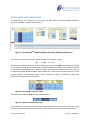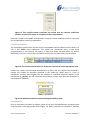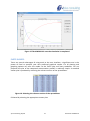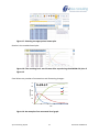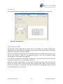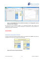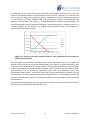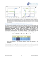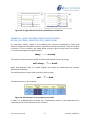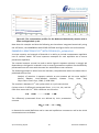
1
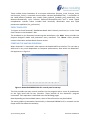
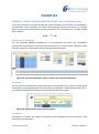
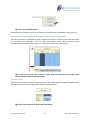
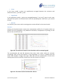
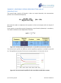
USER MANUAL Reaction Modelling for Kinetic Processes CONTENTS SYSTEM REQUIREMENTS AND INSTALLATION ....................................................................... 3 CONTACT INFORMATION AND SUPPORT .............................................................................. 3 REFERENCE GUIDE ..................................................................................................................... 4 INTRODUCTION ...................................................................................................................... 4 EXAMPLES .............................................................................................................................. 4 EXCEL TEMPLATES .................................................................................................................. 5 STARTING THE MATLAB PROGRAM ....................................................................................... 5 Program Operation ................................................................................................................ 6 Load Excel File .................................................................................................................... 6 Close Excel File ................................................................................................................... 6 MODEL ENTRY AND COMPILATION ....................................................................................... 7 Compile Model ................................................................................................................... 8 Initial Concentrations ......................................................................................................... 9 Constant entry ................................................................................................................... 9 Timebase .......................................................................................................................... 10 Simulate ........................................................................................................................... 11 PLOTS IN EXCEL .................................................................................................................... 12 GRAPH MENU....................................................................................................................... 14 Toggle legend ................................................................................................................... 14 Grid................................................................................................................................... 14 Plot log time ..................................................................................................................... 14 Copy graph to clipboard................................................................................................... 14 Print preview .................................................................................................................... 15 PARAMETER SLIDERS ........................................................................................................... 15 NUMERICAL AND OTHER OPTIONS ...................................................................................... 16 HANDLING PROTONATION EQUILIBRIA, [H], [OH] and Kw .................................................. 17 MODEL ENTRY SYNTAX RULES ............................................................................................. 18 EXAMPLES ................................................................................................................................ 19 Example 1: Simple second order reaction A+B→C (AplusBtoC.xlsx) ................................... 19 Loading the Excel template.............................................................................................. 19 The Model ........................................................................................................................ 19 Jplus Consulting Pty Ltd 2 ReactLab™ KINSIM 1.0 Compilation ...................................................................................................................... 19 Entry of the rate and equilibrium constants and the initial concentrations ................... 20 The time vector ................................................................................................................ 20 Simulate ........................................................................................................................... 21 Example 2: Reversible second order reaction A+B↔C (AplusBeqC.xlsx) ........................... 22 ENZYME KINETICS ................................................................................................................ 23 Example 3: Enzyme kinetics (Enzyme_1.xlsx) ...................................................................... 23 Example 4: Enzyme kinetics revisited (Enzyme_2.xlsx) ....................................................... 24 Example 5: Enzyme kinetics revisited again (Enzyme_3.xlsx) ............................................. 26 Example 6: Lotka-Volterra predator-prey model (Lotka_Volterra_predator_prey_model.xlsx) ...................................................................... 27 Example 7: The Belousov-Zhabotinsky reaction (Belousov-Zhabotinsky.xlsx) .................... 29 Example 8: Reaction of Cu2+ with cyclam (Cu_cyclam.xlsx)................................................. 30 References ........................................................................................................................... 31 SYSTEM REQUIREMENTS AND INSTALLATION Please refer to the ‘System Requirements and Installation Guide’ available on our website, and included with the ReactLab™ download. CONTACT INFORMATION AND SUPPORT [email protected] www.jplusconsulting.com Jplus Consulting Pty Ltd 8 Windsor Road WA 6158, Australia ABN: 83-135-664-603 Jplus Consulting Pty Ltd 3 ReactLab™ KINSIM 1.0 REFERENCE GUIDE INTRODUCTION ReactLab™ KINSIM provides extensive reaction modelling capabilities and allows visualisation and quantitative simulation of complex reaction mechanisms. The program comes in both a free version, ReactLab™ KINSIM, and a licensed version, ReactLab™ KINSIM PLUS. The PLUS version offers extended graphics and visualisation features from the ReactLab GUI and a Parameter Slider feature which allows dynamic adjustments to reaction parameters to be observed interactively. The free version of ReactLab™ KINSIM also limits the available number of reaction steps which can be modelled to six. ReactLab KINSIM ReactLab KINSIM PLUS 6 20 Interactive Parameter sliders No Yes Extended graphics features and print support No Yes Max Reaction Steps In this manual which is applicable to both programs sections referring to features available only in ReactLab™ KINSIM PLUS will be preceded with PLUS START and appended PLUS FINISH The programs, including all algorithms and the GUI front end has been developed in Matlab and compiled to produce the final deployable application. They require the Matlab Compiler Runtime (MCR) library to be installed on the same computer. This allows the programs to run on computers without a standard Matlab installation and is supplied as part of the installation package. Model entry and computational output are organised in Excel Workbooks, which are launched from, and dynamically linked to, the ReactLab™ application. Similarly, all numerical analysis options are organised in the Excel format. It is therefore necessary for Excel to be installed on the same computer as ReactLab™. The benefit of using Excel is that all simulation results can be easily shared and further manipulated using standard Excel tools without further need for ReactLab KINSIM. Excel workbooks are compatible with both the free and PLUS versions of ReactLab KINSIM. The program requires Excel analysis workbooks to retain a strict format, as is provided in the examples and templates. EXAMPLES A selection of example workbooks and a template KINSIM workbook accompanies the program in a subfolder in the installation directory. We recommend you copy this subfolder to your documents library. Feel free to experiment with the parameters in the examples. Jplus Consulting Pty Ltd 4 ReactLab™ KINSIM 1.0 These include three simulations of an enzyme mechanism (Enzyme_1.xlsx, Enzyme_2.xlsx and Enzyme_3.xlsx); a reversible second order reaction (AplusBeqC.xlsx); a simulation of the Lotka-Volterra predator prey model (Lotka_Volterra_predator_prey_model.xlsx); the Belousov-Zhabotinsky cyclic reaction (Belousov-Zhabotinsky.xlsx) and a metal ligand complexation reaction which includes both kinetically observable rates and rapid protonation equilibria (Cu_cyclam.xlsx). EXCEL TEMPLATES To inspect an Excel ReactLab™ KINSIM workbook load it directly into Excel, or via the ‘Load Excel’ button in the ReactLab™ GUI. The workbook is pre-formatted containing two worksheets, the ‘Main’ sheet provides the purpose designed model and parameter entry interfaces. The ‘About’ sheet provides contact information and workbook format version. STARTING THE MATLAB PROGRAM When ReactLab™ is launched it also requires the Matlab MCR to initialise. This can take a while and is very much dependant on computer performance, after which the ReactLab™ GUI appears as in Figure 1. Figure 1: ReactLab KINSIM PLUS GUI control panel at startup This GUI provides the main control interface for the program with a series of pushbuttons on the right hand side for key functions. These provide all the ReactLab™ program commands. Their operation is described over the following pages. Note depending on the workbook status, some of these functions may be disabled. The extra graphics presentation functionality in ReactLab KINSIM PLUS is accessed via the Graph menu item above the toolstrip. Jplus Consulting Pty Ltd 5 ReactLab™ KINSIM 1.0 An About menu item at the top left provide details of the ReactLab™ version and in the case of ReactLab™ KINSIM PLUS important licensing information. PROGRAM OPERATION Load Excel File Press Load Excel File in the ReactLab™ GUI to select and link to an Excel Workbook. This will launch a new instance of Excel and load the requested workbook independent of any other open Excel workbooks. Only the ReactLab™ KINSIM workbook template or already developed spreadsheets can be loaded. Figure 2 shows the opened enzyme_1.xlsx example workbook ‘Main’ worksheet. Figure 2: The Enzyme_1.xlsx workbook Important: Excel is launched as an ActiveX server in an independent process linked to ReactLab™ which communicates with it through its Microsoft component object model (COM) interface. The launch of Excel and ActiveX server linkage is initiated by the Matlab (ReactLab) program. Linking to an already open workbook in Excel is NOT supported. If a workbook is prepared for simulation it should first be saved and re-opened from the running ReactLab™ application. Note all Excel functionality is available to manipulate the workbook as normal while it is linked to ReactLab™. Close Excel File This will close the current workbook and link, prior to opening another. If any changes have been made to the workbook the user must first switch focus to the workbook where he/she will be prompted as to whether the changes to the workbook need to be saved. Jplus Consulting Pty Ltd 6 ReactLab™ KINSIM 1.0 MODEL ENTRY AND COMPILATION To demonstrate the simulation of new data we start with the pre-formatted template, ReactLab_KINSIM_Template (see Figure 3). Figure 3: The ReactLabTM KINSIM template, ReactLab_KINSIM_Template.xlsx The reaction we will model is the simple consecutive reaction scheme k k 2 1 A B C The reaction scheme is entered in the model entry area of the ‘Main’ worksheet, see Figure 4. The species names and reaction types (using drop down list options) are added to the list in the fields headed ‘Reactants’, ‘Reaction Type’ and ‘Products’. Note each reaction step is entered individually A→B and B→C which allows for a one-to-one correspondence of each reaction step to its parameter value in the ‘Parameter’ column. Parameters values and labels are not required for compilation. Figure 4: Entering the A→B→C model A second order reaction A+B→C would be entered as: Figure 5: Syntax for a 2nd order step If the reaction is reversible with individual forward and reveres rates this is entered as two lines using the following syntax. Note the reverse reaction is actually entered ‘backwards’. Jplus Consulting Pty Ltd 7 ReactLab™ KINSIM 1.0 k+ C A + B k- Figure 6: Syntax for a reversible reaction If a reaction comprises a rapid (effectively instantaneous) equilibrium it is entered using the ‘=’ symbol. This is typically the case for protonation equilibria. Figure 7: Using the '=' symbol for a rapid equilibrium In this case the parameter is an equilibrium constant; an equilibrium constant is always entered as its logarithmic (base 10) value. Any fast equilibrium is always entered syntactically as an association constant Kass with the associated product on the right. In addition leading numbers prefixing a species letter or string will be interpreted as stoichiometry coefficient for the species in question e.g. 2A > B. Similarly trailing numbers are used to represent multiple species in a particular complex e.g. ML, ML2, ML3 etc. Essentially, ‘normal’ chemical reaction equations can be used. For further information on the syntax rules see page 18. In all cases a label for each parameter can be provided. This allows easier reference to mechanisms with multiple steps. These labels and the parameter values themselves are not required prior to compilation (see C below). Figure 11 gives an example of annotated rate and equilibrium constants. This relatively simple syntax allows accurate models of realistic complexity to be correctly modelled (see Examples). Important: It is necessary for any new entry in the Excel workbook to be properly completed, i.e. by hitting return or pressing the arrow or return key to take the focus away from the cell in question once the value has been assigned, otherwise the ‘Incomplete worksheet entry’ warning will be raised. Failing to enter values properly prevents ReactLab™ from accessing the worksheet cell through the ActiveX interface. Compile Model When model entry is complete press the Compile Model button. Jplus Consulting Pty Ltd 8 ReactLab™ KINSIM 1.0 Figure 8: The compile button translates the model into the internal coefficient notation required for Kinsim to complete further computations ReactLab™ reads in the model and translates it into an internal coefficient format necessary for its subsequent numerical calculations. Initial Concentrations The compilation process also extracts all the intermediate species names and lists them in a row in the ‘Main’ Excel worksheet. This allows the convenient entry of the initial concentrations to be inserted, see Figure 9. Note that these concentrations are always defined for time zero, not the first time point at which the concentrations are calculated. Figure 9: The initial concentration for all species are entered in the appropriate cells Certain key values are calculated automatically by Excel and are required by ReactLab™, namely the number of reactions specified in the model for which there is a rate or equilibrium constant field (n_par) and the number of individual chemical species in the mechanism (n_species). Do not overwrite the formulae in these cells (they are protected in the templates supplied). Figure 10: Model information automatically generated by Excel Constant entry Prior to simulation estimates or known values for all rate (and equilibrium) constants need to be entered in the appropriate fields (Figure 11). Rates constants are entered as absolute Jplus Consulting Pty Ltd 9 ReactLab™ KINSIM 1.0 values but for equilibrium constants the parameter value must be expressed as its log value; e.g. 3 for Kass=103M-1. Figure 11: Annotated parameter value entry alongside the model in the ‘Main’ sheet Timebase Before the simulation can be completed, information about the time span for which the reaction should be simulated has to be provided. ReactLab KINSIM allows three different modes to define the time vector at which the concentrations will be computed: Linear Logarithmic Manual The preferred time-base mode is selected from the drop-down menu. Figure 12: The time base is chosen from a drop-down menu In the linear mode n_points are chosen equidistantly between the T_min and T_max parameters. In the logarithmic mode each consecutive point is a constant factor times the previous point creating a logarithmin progression of time values. This factor is computed in such a way that there are n_points between the T_min and T_max parameters. In logarithmic mode the initial time point cannot be zero (if a zero value is provided the program will, by default, replace this with 1e-4). In the manual mode the time points can be defined individually in the appropriate column. In this mode the entries for T_min, T_max and n_points are ignored Jplus Consulting Pty Ltd 10 ReactLab™ KINSIM 1.0 Figure 13: Manual entry for a specific time vector Important note: irrespective of the time base and the initial time of the time vector, the initial concentrations defined as in Figure 9, are always defined for time zero. Please note generation of the new time base requires the simulation step (below). Simulate After definition of the model, the initial concentrations and the time vector, the Simulation button starts the computation of the concentration profiles which are written into the appropriate columns of the spreadsheet. Figure 14: The computed concentrations are stored in the appropriate columns The concentration profiles are also displayed in the KINSIM GUI as shown below. Jplus Consulting Pty Ltd 11 ReactLab™ KINSIM 1.0 Figure 15 The KINSIM GUI once the simulation is completed PLOTS IN EXCEL There are several advantages of using excel as the user interface; a significant one is the power of Excel to produce your own preferred graphical output. For all plotting and graphing options we refer the reader to the Excel help and many textbooks. For our purposes the plot of the computed concentration profiles is relatively simple. A standard scatter plot is produced by selecting the relevant section of the spreadsheet: Figure 16: Selecting the relevant section of the spreadsheet Followed by selecting the appropriate scatter plot: Jplus Consulting Pty Ltd 12 ReactLab™ KINSIM 1.0 Figure 17: Selecting the appropriate Scatter plot Results in the standard excel plot: Figure 18: The resulting basic excel Scatter Plot reproducing the KINSIM GUI plot of Figure 15 Excel allows any number of annotations and formatting changes: 0.1 A→B→C concentrations 0.08 A B 0.06 C 0.04 0.02 0 0 10 20 30 40 50 time Figure 19: An example of an annotated Excel graph Jplus Consulting Pty Ltd 13 ReactLab™ KINSIM 1.0 PLUS START GRAPH MENU This menu is disabled in the free version of KINSIM and is available above the toolbar on the KINSIM PLUS GUI. Figure 20: The Graph Menu in KINSIM PLUS Toggle legend Plots the figure legend outside the graphics area to improve trace visibility. Grid Plots a grid on the graphics background. Plot log time Switches between logarithmic and linear display of the time base. Figure 21: KINSIM graphs with grid and logarithmic time base Copy graph to clipboard Copy the graph to the clipboard and a Windows meta-file which can then be directly pasted to other documents. Jplus Consulting Pty Ltd 14 ReactLab™ KINSIM 1.0 Print preview Print preview display allowing the graph to be resized and positioned prior to printing. Figure 22: Print preview PARAMETER SLIDERS The parameter slider dialog box (see Figure 23) is only available as a feature of ReactLab™ KINSIM PLUS and allows dynamic simulation of the concentration profiles while interactively adjusting the parameters using the sliders. Each rate or equilibrium parameter has a slider which allows the adjustment of the value. As soon as the change is made the corresponding values in the Excel workbook change accordingly and all the graphs are updated. If a new value is entered in the edit box the sliders are re-centred around this new value. In this way the range span can be changed as required. Note the rate value slider position is not centred since the span range is set to be from one fifth of the current value to five times the value and the slider range is linear (from the minimum to maximum). Conversely, the sliders are central for the logK parameters as these are adjustable by plus or minus five. Jplus Consulting Pty Ltd 15 ReactLab™ KINSIM 1.0 Figure 23 The KINSIM GUI, Excel workbook example in the background and the Parameter Slider Dialog box. The main use of the parameter sliders is to conveniently observe how sensitive the concentration profiles are to the various parameters involved and to see the effects of adjustments to them interactively. PLUS FINISH NUMERICAL AND OTHER OPTIONS A range of numerical calculation and other options are provided in the ‘Main’ sheet that can be adjusted. There are also a number of software flags. Figure 24: The array of option definitions Jplus Consulting Pty Ltd 16 ReactLab™ KINSIM 1.0 Numerical Several of the numerical options and are included for completeness rather than intended for routine customer use. Numerical Integration Stiff solver: This is switches the numerical integration routine used during the calculation of concentration profiles during update or fitting. It is relevant when very large differences in rates of change occur in concentration profiles. Particularly with multistep reactions with fast second order interactions. The standard solver is a 4 th order Runga-Kutta which is usually reliable and fast, but under stiff conditions can slow down significantly. If the numerical integration takes too long ReactLab issues a warning and suggest a switch the stiff solver. If you suspect you are facing a stiff problem select the Stiff solver option or indeed select it by default prior to saving the workbook. Abs tol/Rel tol: Used to determine tolerances in the numerical integration calculations. Equilibrium Speciation Conv tol/Max Iter: Used for speciation calculations by Newton Raphson algorithm. Only relevant for models with rapid equilibria. Miscellaneous logKw: This is an advanced feature and allows adjustment of the log of the ionic product of water Kw (1.00x10⁻¹⁴M2) if required. LogKw is -14 for pure water at room temperature but changes with mixed solvents, ionic strength and temperature. This equilibrium is included when modeling reactions involving protonation equilibria to correctly deal with [H] and therefore pH. See below for more details. HANDLING PROTONATION EQUILIBRIA, [H], [OH] AND KW In some cases reaction models in aqueous solution may include protonation equilibria. In such instances the autoprotolysis of water has to be taken into account. This is done automatically by ReactLab™ if any of the components in the system is identified as ‘H’ which is interpreted as a proton. This is one of the very few rules about the names of components or species in ReactLab™. As a consequence of the presence of protons it is assumed that the reaction is performed in aqueous solution and the equilibrium KW H2O H+ + OH- is internally added to the present model. Further the hydroxide, OH, will be added automatically to the list of species. The ionic product Kw is represented as: KW = [H+ ] [OH- ] Jplus Consulting Pty Ltd 17 ReactLab™ KINSIM 1.0 The unionized water is omitted from the expression as its concentration is essentially constant. The value of KW is then 1.00x10⁻¹⁴ M2 for pure water at room temperature. If measurements are taken at a different temperature, solvent or ionic strength the correct value for logKw is stored in cell ‘I55’ of the ‘Main’ worksheet. If protons are involved in a process and the autoprotolysis of water should not be implemented automatically, an easy option is to call it ‘P’ or anything but ‘H’. MODEL ENTRY SYNTAX RULES A kinetic reaction step is indicated by the symbol ">", e.g.: A+B>C The parameter associated with “>” is a rate constant (1st or 2nd order). Reversible kinetic steps (slow equilibria) are expressed over two lines i.e. A+B>C C>A+B In this case both forward and reverse rate constants are independently defined and can be fitted. A rapid (instantaneous) equilibrium is indicated by "=". The parameter associated with “=” is an equilibrium constant K. This can be fitted but the microscopic forward and reverse rates are not accessible. The parameter when "=" is used for an equilibrium is log10 of the association equilibrium constant, logK. Note this means it can be negative or positive depending on whether the equilibrium constant itself is less or greater than 1. Each equilibrium can only have one product. No two equilibria can have the same product. Reactants and products within a particular step are combined using the "+" symbol. Species names can be single or multiple characters. The stoichiometries of species in a particular step are indicated by an integer to the left of the species name (no integer is assumed to mean a stoichiometry of 1). The species name ‘H’ is treated as a special case and if present will enable the automatic incorporation of calculations to account for the autoprotolysis of water. In this situation ‘OH’ will also be added to the participating species list. In this version of ReactLab™ OH cannot participate in a kinetic step – only in the auto- equilibrium with H (above) Thus equilibria can be incorporated into a reaction model in two ways. They can be expressed as kinetically observable forward and back reactions, each by using ">" symbol, allowing the individual rates to be potentially fitted. Alternatively they can be expressed as equilibria, using the “=” symbol, where the equilibration is instantaneous at any particular time. In this case the equilibrium is defined by its equilibrium constant and the concentrations of the equilibrium species at a particular time are determined using the law of mass action. This mode of calculation is particularly suited to equilibria where equilibration is so rapid that it cannot be observed (e.g. protonation equilibria). Jplus Consulting Pty Ltd 18 ReactLab™ KINSIM 1.0 EXAMPLES EXAMPLE 1: SIMPLE SECOND ORDER REACTION A+B→C (AplusBtoC.xlsx) In this first example we will go through the steps of setting up the model, the compilation, the definition of the constants, the initial concentrations and the time vector of reaction times at which the concentrations will be computed. The first example is a simple second order reaction: k A +B C Loading the Excel template The file ‘ReactLab_KINSIM_Template.xlsx’ is the template into which the information required for the simulation is entered. After these entries, it is saved under a different name and then ready for re-opening for further changes and simulations. Figure 25: The Excel Template, ready to receive the relevant information The Model The first step is to define the reaction mechanism or the model; this is done by entering the information into the appropriate cells of the Excel spreadsheet. The ReactLab model entry is very flexible and allows the notation that chemists would use on paper. Figure 26: Model entry for the reaction A+B→C Compilation Compilation translates the model as defined in the spreadsheet into the internal code required by the algorithms Jplus Consulting Pty Ltd 19 ReactLab™ KINSIM 1.0 Figure 27: The compile button Compilation also defines the list of all species in row 30 of the spreadsheet, see Figure 28. Entry of the rate and equilibrium constants and the initial concentrations The rate constants are defined for each reaction in column F and the initial concentrations for all species are entered in row 31 under the species names. Note that the initial concentrations are defined for time zero, not the first time in the time vector. Figure 28: Entry of the rate constant in line with the reaction and of the initial concentrations under the species names The time vector There are three options to define the time vector, the Select type drop-down window allows the choice between linear, logarithmic, and manual definition. Figure 29: Three options to define the time vector Jplus Consulting Pty Ltd 20 ReactLab™ KINSIM 1.0 Linear In the linear mode, n_points are equidistantly arranged between the minimum and maximum times, T_min and T_max. Logarithmic In the logarithmic mode, n_points are arranged between T_min and T_max in such a way that each time point is a constant factor times the preceding time. Note that T_min cannot be zero. Manual Any arbitrary time vector with increasing points can be defined in the manual mode. Simulate Clicking the Simulate button creates the concentration profiles for all species which are written into the spreadsheet. Any additional calculation, manipulation or plotting can be done in the normal Excel way. Figure 30: The numerical output of the Simulation with an example graph The concentration [A] and [B] decrease from their initial values while [C] increases accordingly. After 50 sec the reaction is still proceeding, it is easy to re-define the time vector and simulate a longer time span. After 200 sec, the concentration of the minor starting material has essentially reached zero and the reaction is finished. 1.20E-01 1.00E-01 8.00E-02 A 6.00E-02 B C 4.00E-02 2.00E-02 0.00E+00 0.000 50.000 100.000 150.000 200.000 250.000 Figure 31: The same reaction simulated for 200 sec. Jplus Consulting Pty Ltd 21 ReactLab™ KINSIM 1.0 EXAMPLE 2: REVERSIBLE SECOND ORDER REACTION A+B↔C (AplusBeqC.xlsx) The second order reaction of Example 1 does not require ReactLab, the concentration profiles can be calculated analytically. [A] = [A]0 ([B]0 - [A]0 ) [B]0 e([B]0 -[A]0 )kt - [A]0 ([A]0 [B]0 ) We invite the reader to implement the equations in Excel and compare with the output of ReactLab. If the reaction is reversible numerical integration, as performed by ReactLab, is mandatory. The model is defined in two independent reactions. k + C A +B k- Figure 32: The ReactLab model definition for a reversible second order reaction The concentration profiles are different and the equilibrium position is reached in some 20 sec. The equilibrium constant for the rate constants above is of course 10, K=k+/k-. 1.20E-01 1.00E-01 8.00E-02 A 6.00E-02 B C 4.00E-02 2.00E-02 0.00E+00 0.000 10.000 20.000 30.000 40.000 50.000 60.000 Figure 33: The concentration profiles for the reversible second order reaction Jplus Consulting Pty Ltd 22 ReactLab™ KINSIM 1.0 ENZYME KINETICS EXAMPLE 3: ENZYME KINETICS (Enzyme_1.xlsx) Figure 34 displays the ‘Main’ worksheet (Enzyme_1.xlsx) which models the interaction of the substrate S with the enzyme E and subsequent irreversible product formation. k k2 k3 1 ES E + S EP E +P k-1 To see the simulation in the KINSIM GUI select ‘Compile’ and then ‘Simulate’ in the GUI. This is necessary to initialise ReactLab with the model in the workbook and then simulate it according to the initial parameters and timebase. In the first reversible step the enzyme reacts with the substrate to form the intermediate ES which subsequently forms, in an irreversible step, the enzyme product complex EP which in turn decays, also irreversibly, to release the product P and the enzyme which can start another cycle. The advantage of KINSIM is that it can be used to simulate enzyme kinetics under both steady state conditions (see Example 4 below) and to investigate the pre-steady state behaviour when substrate and enzyme first interact. Under steady state conditions high substrate and catalytic enzyme concentrations mean the enzyme bound intermediates are rapidly saturated and remain approximately constant until the substrate is exhausted. Historically this was the only practical way enzyme reactions could be studied and provided the foundation of the development of the steady state assumption and Michealis-Menten kinetic analysis quantifying enzyme behaviour in terms of KM and kcat. No information was available to elucidate the details and specific kinetic events of the underlying enzyme mechanism. We will illustrate this further in later examples. One of the reasons analysis was restricted in this way was because of the limited availability of purified enzyme and insufficiently sensitive kinetic detection technologies. When protein purification improved and enzymes could be produced in larger amounts experiments could be conducted which allowed the formation of enzyme intermediates during the pre-steady state phase to be observed. This also required the development of instrumental techniques such a stopped-flow coupled in particular to highly sensitive fluorescence detection. For further information on the emergence of pre-steady state kinetics and a thorough discussion of the evolution of the study of enzyme kinetics the reader is referred to the references of Fersht and Gutfreund. Fortunately, simulation and modelling of these processes is not hampered by experimental constraints. In a so-called single-turnover experiment we can ‘observe’ the kinetics during an experiment where the substrate and enzyme concentrations are similar ([E]0=10-5M, [S]0=2×10⁻⁵M). For the given initial concentrations ([E]0=10-5M, [S]0=2×10⁻⁵M) and rate constants (k1=106M-1s-1, k-1=10s-1, k2=2s-1 and k3=4s-1) the first fast step is the formation of the ES complex, this phase of the reaction takes about 100 msec. The next phase consists of the transformation of the ES into the EP intermediate which in turn reacts further to release the product. The complete transformation of the substrate takes about 5 sec; at that time Jplus Consulting Pty Ltd 23 ReactLab™ KINSIM 1.0 the enzyme is also released completely and reaches the initial concentration while the product reaches the initial concentration of the substrate. ReactLab KINSIM calculates the concentration profiles for the predefined timespan and stores them in the columns B to G; they can be plotted in Excel in the usual way. Figure 34: The Enzyme_1.xlsx example workbook It is worthwhile noting that the concentrations seen in the above example are often not observable in traditional absorption spectroscopy. In contrast, fluorescence emission spectroscopy can be much more sensitive and for some substrates the above reactions can be observed (see Gutfreund). EXAMPLE 4: ENZYME KINETICS REVISITED (Enzyme_2.xlsx) In this example we continue with the same enzymatic mechanism but explore its bahaviour under different conditions. k k2 k3 1 ES E + S EP E +P k-1 The initial concentration of enzyme, E, and substrate, S, were previously chosen to demonstrate the initial interactions to form the first and second intermediates, ES and EP, and the final product, P. This was a so-called single-turnover or pre-steady-state experiment. Such small concentrations for the substrate enable the pre-steady state transient kinetics to be observed and the mechanism dissected but now we will see how the system behaves under more biologically relevant steady state conditions. In this example we use the same rate constants but have an initial substrate concentration of 0.01 M, the initial enzyme concentration is still 10 -5 M. Plotting the concentration of substrate and product reveals the classical pseudo-zeroth order kinetics: a linear decrease Jplus Consulting Pty Ltd 24 ReactLab™ KINSIM 1.0 of substrate with the concomitant linear increase in the product concentration. This is the result of the limited amount of enzyme which turns over the substrate at a constant rate until it runs out. Under these conditions there is negligible free enzyme during this phase as it is all bound in the form of ES and EP, and the enzyme reaction is proceeding at the maximum rate possible. This is the Vmax in Michaelis-Menten steady state terminology. The rate of continuous product formation during this steady state phase is known as the kcat or turnover number of the enzyme (=Vmax/[E]0) which quantifies how much substrate is converted to product per second. 1.20E-02 1.00E-02 8.00E-03 E S 6.00E-03 ES EP 4.00E-03 P 2.00E-03 0.00E+00 0 200 400 600 800 1000 1200 Figure 35: Pseudo first-order enzyme kinetics, linear decreased and increase of substrate and product The next Figure reveals some interesting details of the simulation. Part a) only shows the profiles for the enzyme and the two intermediates (this requires a highly zoomed-in y-axis to be seen in the ReactLab GUI). Clearly visible is the long section where the concentrations of the intermediates are almost perfectly constant; this of course is the well-known steadystate situation. Part b) features a logarithmic time scale. The formation of the first intermediate takes about 1 msec after which the enzyme concentration reaches very low concentration it is almost quantitatively transformed into the first intermediate. After about 1 sec the transformation into the second intermediate has progressed to the steady-state concentrations. This Figure also demonstrates the ease by which such plots can be created in Excel. We refer to user to many textbook and help files for Excel. Jplus Consulting Pty Ltd 25 ReactLab™ KINSIM 1.0 1.20E-05 1.20E-05 a) 1.00E-05 b) 1.00E-05 8.00E-06 8.00E-06 E 6.00E-06 E 6.00E-06 ES EP 4.00E-06 ES EP 4.00E-06 2.00E-06 2.00E-06 0.00E+00 0.00E+00 0 200 400 600 800 1000 1200 0.000001 0.0001 0.01 1 100 Figure 36: a) the concentration profiles of the intermediate enzyme complexes demonstrate the steady-state behavior; b) a logarithmic time scale reveals the very fast formation of the first intermediate and transformation into the second intermediate. EXAMPLE 5: ENZYME KINETICS REVISITED AGAIN (Enzyme_3.xlsx) The initial interaction between the enzyme and the substrate is very fast and normally not observable. It is then not possible to determine the individual values for the forward and back rate constants (k1 and k-1) and it makes sense to define this first step as an instantaneous equilibrium. ReactLab allows the definition of such equilibria very straightforwardly. The ‘=’ sign in the Reaction Type cell defines the reaction as an, instantaneous, equilibrium. Note that equilibrium constants in the parameter cells are always defined as their logarithms to the base of 10. K1 = k1/k-1 = 106/10 = 105; logK1 = 5. K k2 k3 1 ES E +S EP E +P Figure 37: Definition of the interaction between enzyme and substrate as an equilibrium Comparing Figure 36 with Figure 38 reveals that the concentration profiles are essentially indistinguishable, apart from the first msec where the E+S interaction takes place for the kinetic definition. Here the establishment of the equilibration is instantaneous. Jplus Consulting Pty Ltd 26 ReactLab™ KINSIM 1.0 1.20E-05 1.20E-05 a) 1.00E-05 b) 1.00E-05 8.00E-06 8.00E-06 E 6.00E-06 E 6.00E-06 ES EP 4.00E-06 ES EP 4.00E-06 2.00E-06 2.00E-06 0.00E+00 0.00E+00 0 200 400 600 800 1000 1200 0.000001 0.0001 0.01 1 100 Figure 38: as Figure 36 with the first step defined as equilibrium EXAMPLE 6: LOTKA-VOLTERRA PREDATOR-PREY MODEL (LOTKA_VOLTERRA_PREDATOR_PREY_MODEL.XLSX) An interesting ‘kinetic’ model is the predator-prey ‘reaction’ developed by Lotka and Volterra. Imagine an island with a certain population of sheep and wolves. There are several ‘reactions’: in a first ‘reaction’ the sheep breed, relying on grass as their feed. The reaction is, of course, biologically not quite correct: k 1 sheep 2 sheep The wolves of the island also multiply but they need sheep as source of energy k 2 wolf + sheep 2 wolf (Note that ReactLab does not ‘speak’ English and would not understand the reaction wolf+sheep→2wolves.) The wolf population is kept under control by wolves dying k 3 wolf dead The ReactLab entry is just as above Figure 39: Model entry for the predator-prey model In Excel it is straightforward to delete the ‘concentration profile’ of the dead wolves to reveal the perfect cyclic behavior of this ‘reaction’. Jplus Consulting Pty Ltd 27 ReactLab™ KINSIM 1.0 3.5 3 2.5 2 sheep 1.5 wolf 1 0.5 0 0 2 4 6 8 10 Figure 40: The completely cyclic behavior of the Lotka-Volterra predator-prey model Figure 41: The ReactLab KINSIM window with the concentration profiles. The Parameter slide GUI of ReactLab KINSIM PLUS allows the convenient change of any of the rate constants Jplus Consulting Pty Ltd 28 ReactLab™ KINSIM 1.0 EXAMPLE 7: THE BELOUSOV-ZHABOTINSKY REACTION (BelousovZhabotinsky.xlsx) The Belousov-Zhabotinsky reaction is a famous cyclic reaction. In contrast to the predatorprey model before this reaction one is real. However, the reaction mechanism is not completely understood and a simplified version that is usually used to describe the chemical reaction is chemically/stoichiometrically not quite correct. The Belousov-Zhabotinsky (BZ) reaction involves the oxidation of an organic species such as malonic acid (MA) by an acidified aqueous bromate solution in the presence of a metal ion catalyst such as the Ce(III)/Ce(IV) couple. At excess [MA] the stoichiometry of the net reaction is catalyst 2BrO-3 +3CH2(COOH)2 +2H+ 2BrCH(COOH)2 +3CO2 +4H2O A reasonable approximation for the cyclic behavior results from the following reaction mechanism. k1 BrO-3 +Br- HBrO2 +HOBr k 2 BrO-3 +HBrO2 2HBrO2 +2Mox k3 HBrO2 +Br- 2HOBr k4 2HBrO2 BrO-3 +HOBr k5 MA+Mox 12 Br- With rate constants and initial concentrations as defined in the spreadsheet in Figure 42 the cyclic behavior of Figure 43 results. Figure 42: the Belousov-Zhabotinsky reaction in ReactLab The numerical integration delivers the concentration profiles for all species. Figure 43 a) demonstrates the slow conversion of the malonic acid and bromate to HOBr. The oscillations for the remaining species are not visible as the concentrations are too low. Using a logarithmic concentration axis reveals the oscillations, Figure 43 b). Jplus Consulting Pty Ltd 29 ReactLab™ KINSIM 1.0 1.00E+00 0.3 a) 0.25 BrO3 0.2 b) 1.00E-01 Br 1.00E-02 1.00E-03 HBrO2 0.15 HOBr 0.1 0.05 1.00E-04 Mox 1.00E-05 MA 1.00E-06 Bri 1.00E-07 1.00E-08 0 0 200 400 600 800 0 1000 200 400 600 800 1000 Figure 43: The concentration profiles for the Belousov-Zhabotinsky reaction with a linear and logarithmic y-axis Note that this example and also the following one have been integrated numerically using the stiff solver, see NUMERICAL AND OTHER OPTIONS and Figure 24 for more information. EXAMPLE 8: REACTION OF CU2+ WITH CYCLAM (Cu_cyclam.xlsx) A unique capacity and strength of ReactLab is its ability to include instantaneous equilibria into its reaction model. The most important examples for such equilibria are of course protonation equilibria. The reaction between a metal ion and an amine ligand in aqueous solution is strongly pH dependent as the ligand is involved in one or several protonation equilibria. Each differently protonated form will react with the metal ion with different rate constants. The following example is taken from the literature, the publication where the above idea is published the first time Analysis of reactions in aqueous solution at non-constant pH: No more buffers? Marcel Maeder, Yorck-Michael Neuhold, Graeme Puxty, Peter King Phys. Chem. Chem. Phys., 2003, 5, 2836-2841 The reaction is between Cu2+ and cyclam which is a cyclic tetra-amine. Cyclam exists in 5 differently protonated forms, L, LH, LH2, LH3, and LH4. Each form reacts with Cu2+ with a different rate constant kLHx 2+ Cu2+ + LHx+ + xH+ x CuL N N N N The differently protonated forms are defined by their protonation constant Kx LH(x-1)+ + H+ LHxx x-1 In ReactLab the model definition and its rate and equilibrium constants as well as the initial concentrations are as follows. Jplus Consulting Pty Ltd 30 ReactLab™ KINSIM 1.0 Figure 44: The model for the reaction of Cu2+ with cyclam. The modelling results in the same concentration profiles as in Figure 3(b) of the above publication. 3.5 0.006 3 0.005 pH 2.5 2 ML pH concentration 0.004 0.003 1.5 0.002 LH2 0.001 1 M 0.5 LH4 0 0 LH3 0 5000 10000 15000 20000 25000 30000 time Figure 45: The resulting concentration profiles REFERENCES Marcel Maeder, Yorck-Michael Neuhold. Practical Data Analysis in Chemistry, Elsevier 2007 Jplus Consulting Pty Ltd 31 ReactLab™ KINSIM 1.0 John Ross, Igor Schreiber, Marcel O. Vlad, and Adam Arkin. Determination of Complex Reaction Mechanisms: Analysis of Chemical, Biological, and Genetic Networks. Oxford University Press 2005 Robert W. Hay. Reaction Mechanisms of Metal Complexes. Albion/Harwood Pub 2000 H. Gutfreund. Kinetics for the Life Sciences. Cambridge University Press 1995 James H Espenson. Chemical Kinetics and Reaction Mechanisms (2nd edition). McGraw-Hill 1995 S.K. Scott. Oscillations, Waves, and Chaos in Chemical Kinetics. Oxford. Oxford Chemistry Press 1994. Ralph G. Wilkins. Kinetics and Mechanisms of Reactions of Transition Metal Complexes. VCH 1991 A. Fersht. Enzyme Structure and Mechanism. Freeman 1985 S.W. Benson. The Foundations of Chemical Kinetics. McGraw-Hill New York 1960 Jplus Consulting Pty Ltd 32 ReactLab™ KINSIM 1.0