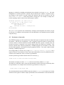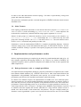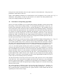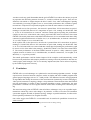
1
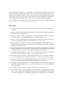
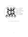
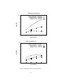
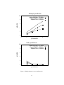
CuPit-2: Portable and Efficient High-Level Parallel
Programming of Neural Networks
Holger Hopp, Lutz Prechelt ([email protected])
Universität Karlsruhe, Fakultät für Informatik, D-76128 Karlsruhe, Germany
Phone: +49/721/608-7344, Fax: -7343
12th January 1998
Submission to the Special Issue on ”Simulation of Artificial Neural Networks”
for the Systems Analysis Modelling Simulation (SAMS) journal
Abstract
CuPit-2 is a special-purpose programming language designed for expressing dynamic neural
network learning algorithms. It provides most of the flexibility of general-purpose languages
such as C or C++, but is more expressive. It allows writing much clearer and more elegant
programs, in particular for algorithms that change the network topology dynamically (constructive algorithms, pruning algorithms). In contrast to other languages, CuPit-2 programs
can be compiled into efficient code for parallel machines without any changes in the source
program, thus providing an easy start for using parallel platforms. This article analyzes the
circumstances under which the CuPit-2 approach is the most useful one, presents a description of most language constructs and reports performance results for CuPit-2 on symmetric
multiprocessors (SMPs). It concludes that in many cases CuPit-2 is a good basis for neural
learning algorithm research on small-scale parallel machines.
Keywords: neural networks, parallel programming, portability, compiler, constructive algorithms,
pruning.
1 Neural network simulation: Requirements and approaches
For simulating artificial neural networks for engineering purposes, there are typically three major
requirements for the simulation system: ease of use, high performance (i.e., execution speed), and
flexibility.
We discuss for which sorts of users which of these requirements are most important, what solutions
are available, and what consequences these solutions have:
1. Ease of use. For rapid development of a neural network solution for a given application
problem (solution engineering) the most important requirement is often to reduce the amount
of human work involved. Hence, the simulation system should allow for simple data handling,
training setup and control, and interactive investigation of strengths and weaknesses of alternative
networks, algorithms, data encodings etc. for the given problem. Furthermore, the software should
be easy to learn.
This sort of requirement is usually best handled by integrated neural network simulators such as
SNNS [23], Xerion [19], NeuroGraph [22], NeuralWorks [11] etc. These programs package multiple well-known learning algorithms with data manipulation functions and interactive graphical
network exploration and manipulation capabilities. They are relatively easy to learn and will often
provide the fastest path to a reasonable solution of a given engineering problem.
The disadvantages of simulators are limited flexibility and often also suboptimal execution speed:
When algorithms beyond the supplied standard ones need to be employed, both ease of use and
ease of learning break down, because internal simulator programming is required. Furthermore,
integrated simulators rarely provide full access to the fastest means of network execution as discussed in the next paragraph.
2. High execution speed. If the networks required for the given learning problem are very large
or there are very many examples, execution speed becomes a dominant factor. In this case, the
simulation system must be optimized for exploiting available hardware performance.
There are three ways for obtaining fast neural network performance: using machine-dependent,
highly optimized libraries for matrix operations, utilizing parallel processors, or employing specialpurpose hardware.
All three kinds of solutions (which may be combined) typically either suffer from limited flexibility or lack ease of use. Not all kinds of learning algorithms can be implemented using given matrix
libraries or special-purpose hardware, the latter may also suffer from problems with computational
precision for some problem domains [20]. On the other hand, general-purpose parallel processors
are quite flexible, yet are typically difficult to program.
3. Flexibility. If one is doing research in neural network learning algorithms or very advanced
development, standard algorithms and network structures may be insufficient; the same is true if
the neural network has to be interwoven (as opposed to interfaced) with other parts of a system.
The worst case are learning algorithms that change the topology of the neural network dynamically during the learning process. We call such algorithms constructive algorithms; they may be
either additive (adding nodes or connections), subtractive (pruning nodes or connections), or both.
Constructive algorithms make network handling very complicated for the simulation system.
In this case, most users end up with handwritten programs in conventional programming languages
such as C or C++. Sometimes, special neural network libraries such as MUME [6] or Sesame [10]
may be used to simplify parts of the programming.
Obviously such flexibility requirements impede or even contradict ease of use. Unfortunately
constructive algorithms also require immense effort for obtaining high execution speed, because
the resulting networks are both irregular and nonstatic; the problem is most pronounced on parallel
computers.
The present paper presents a simulation system based on a special-purpose programming language,
CuPit-2. The system is flexible enough for doing research into constructive learning algorithms,
2
yet allows for exploiting parallel hardware in a machine-independent, portable fashion. Furthermore, the language is problem-oriented and therefore relatively easy to use.
The next section discusses the general idea behind our approach. Subsequent sections informally
present the CuPit-2 language, its implementations, and benchmark results on symmetric multiprocessor machines.
2 The CuPit-2 approach
Our work assumes the following requirements profile:
The user wants to perform research or advanced development of learning algorithms that
modify the topology of the network during the learning phase (constructive algorithms).
To do this, the user will write appropriate simulation programs that implement the new
algorithms.
The user wants to employ general-purpose parallel computers for (some of) the simulations.
The simulation programs must be portable. Their parallel execution should be efficient.
The user is not willing to learn machine-dependent or low-level parallel programming constructs in order to write the simulation programs.
The goal of our work is to provide a simulation system that fits these requirements well. Obviously none of the simulation systems common today fulfills all three requirements: The available
preprogrammed simulators cannot accommodate constructive algorithms, at least not on parallel
machines. The same is true for neural network library approaches. Handwritten implementations
in standard languages such as C or C++ require low-level parallel programming (data distribution,
message passing, work partitioning, thread management, load distribution, etc.) and typically
result in non-portable programs. Finally, high-level general-purpose parallel languages (e.g. Concurrent Aggregates [3]) would be acceptable from the programming point of view, but they cannot
yet be translated into sufficiently efficient parallel code.
Thus we propose to use a special-purpose parallel programming language for neural network learning algorithms. Such a language could be sufficiently simple to learn, because the users understand the abstractions behind its constructs well. It can be made flexible enough to accommodate
constructive algorithms, yet would be completely problem-oriented, thus providing portability
between various parallel and sequential machines. And it could allow for efficient parallel implementation, because knowledge about the behavior of the programs can be built into the compiler
for a special-purpose language.
We have designed a language, called CuPit-2, with these properties. CuPit-2 describes networks
in an object-centered way using special object types “connection”, “node” and “network”. It has
special operations for manipulating network topology and allows for parallel operations by parallel
procedure calls at the network, node group, and connection level.
3
Various proposals for network description languages, often with less clear aims, have been made
by other researchers, e.g. [2, 8, 7, 9, 21]. Most of these cover only static network topologies
and are not full programming languages, thus still exhibit most of the problems of hand-written
implementations. The most advanced of the above proposals is CONNECT [8], which represents a mostly complete programming language, but still has only incomplete support for dynamic
changes of network topology.
3 CuPit-2 language overview
The programming language CuPit-2 [5] views a neural network as a graph of nodes and connections. In the neural network literature, the nodes are often called units or neurons, the connections
are often called links or, misleadingly, weights.
CuPit-2 is based on the observation that neural algorithms predominantly execute local operations
(on nodes or connections), reductions (e. g. sum over all weighted incoming connections) and
broadcasts (e. g. apply a global parameter to all nodes). Operations can be described on local
objects (connections, nodes, network replicates) and can be performed group-wise (connections
of a node, nodes of a node group, replicates of a network, or subsets of any of these). This
leads to three nested levels of parallelism: connection parallelism, node parallelism and example
parallelism. There is usually no other form of parallelism in neural algorithms, such that we can
restrict parallelism to the above three levels without loss of generality.
Modifications of the network topology can also be performed in parallel, either by local operations
(a node splitting or deleting itself, a connection deleting itself) or by global operations (enlarging
or reducing a node group, creating or deleting the connections between two node subgroups).
CuPit-2 is a procedural, object-centered language; there are object types and associated operations
but no inheritance or polymorphism. The identification of network elements is based on four
special categories of object types: connection, node, node group, and network types. A simplified
view of the CuPit-2 network model is shown in the example in Figure 1. CuPit-2’s connections
are always directed, but that does not restrict the flow of information through them.
Fig. 1 !!!
This approach makes a wealth of information readily available to the compiler that would be
difficult to extract from a similar program in a normal parallel programming language. We use
this information to generate efficient parallel and sequential code.
The rest of this section will describe the main parts of a CuPit-2 program consisting of connection, node, and network descriptions (including operations) and a main program that controls the
algorithm.
3.1 Connections
Let us start with an example definition of a connection type that handles weight multiplication
and weight pruning. The following declaration defines a connection type Weight for connecting
two nodes of type SigmoidNode. More precisely: an OUT interface of a SigmoidNode with
4
an IN interface of another (or the same) SigmoidNode. The node type SigmoidNode and its
interfaces will be introduced below.
TYPE Weight IS CONNECTION
FROM SigmoidNode OUT out;
TO
SigmoidNode IN in;
Real weight := 0.0, delta := 0.0;
Real FUNCTION weightMultOutput () IS
RETURN ME.weight * out.data;
END FUNCTION;
PROCEDURE prune (Real CONST threshold) IS
IF abs(ME.weight) < threshold
THEN REPLICATE ME INTO 0; (* self-delete *)
END;
END PROCEDURE;
(* further connection procedures are not shown *)
END TYPE;
As mentioned before, connections are always directed, i. e. , there are no connections between
A and B, but from A to B, so the compiler can co-locate connection data with node data on the
processors of a parallel machine. Nevertheless, data can always be sent along a connection in both
directions.
The Weight connection object is a structure of two data elements weight and delta of the
built-in type Real. Associated with this type are its object functions and procedures. The function weightMultOutput yields the product of the weight with the data element of the
connected FROM node (named out, because it is the out interface of the node). ME always designates the object for which the current procedure is being called.
The prune procedure implements a local topology modification, namely the conditional selfdeletion of the connection. To delete a connection, the connection replicates itself into 0 copies of
itself; the same can be done for nodes including all their connections. Both routines can only be
called from nodes that have connections of type Weight attached, as in the following node type
example.
3.2 Nodes
This is an example definition of a node type that handles forward propagation and connection
pruning.
TYPE SigmoidNode IS NODE
IN Weight in;
OUT Weight out;
Real data, bias;
5
PROCEDURE forwardHidden () IS
Real VAR inData;
REDUCTION ME.in[].weightMultOutput():rsum
INTO inData;
ME.data := activation (inData + ME.bias);
END PROCEDURE;
PROCEDURE prune (Real CONST threshold, Bool CONST hasoutputs) IS
ME.in[].prune (threshold);
(* delete hidden nodes that have become unconnected: *)
IF hasoutputs AND
(MAXINDEX (ME.in[]) < 0 OR MAXINDEX(ME.out[]) < 0) THEN
REPLICATE ME INTO 0;
END;
END PROCEDURE;
(* further node procedures are not shown *)
END TYPE;
The node type SigmoidNode has two data elements, data and bias, and two connection interfaces: in for incoming connections of the above type Weight and out for outgoing connections.
Node procedures operate on all connections attached to an interface at once. For instance the node
procedure prune calls the connection procedure prune on all connections attached to the in
interface of the node. The [] notation stands for “all” and designates parallel calls.
The connection procedure prune is executed in asynchronous parallel fashion for every connection. This call realizes nested parallelism, as the node procedure prune itself may be executed
for several nodes in parallel as well.
To delete a node, the node replicates itself into 0 copies of itself; the same construction is shown
above for connections. MAXINDEX returns the number of objects in a compound object, minus
one (here: the number of connections attached to a connection interface).
The REDUCTION statement in the node procedure forwardHidden combines the results of
weightMultOutput of all connections attached to the in interface using the reduction operator rsum, which is defined by the user as
Real REDUCTION rsum NEUTRAL 0.0 IS
RETURN (ME + YOU);
END REDUCTION;
The result is written into the variable inData and will be the NEUTRAL value of the reduction
operator if there are no connections. The order in which the individual reduction operations (here:
additions) are executed is not defined. Arbitrary reduction operators on arbitrary data types can be
defined in the above manner and will be translated into efficient parallel tree reduction implementations.
The activation function called above is a so-called free subroutine: it is not attached to any
object type and can be called from anywhere.
6
3.3 Networks
Now we will construct a network of SigmoidNodes and their Weight connections:
TYPE Layer
Real
IO
IS GROUP OF SigmoidNode END;
xIn, xOut;
(* I/O-areas, managed externally *)
TYPE Mlp IS NETWORK
Layer
inL, hidL, outL;
Real
totError;
(* three groups of nodes *)
(* total sum squared error *)
PROCEDURE createNet (Int CONST inputs, hidden, outputs) IS
EXTEND ME.inL BY inputs;
(* create input node group *)
EXTEND ME.hidL BY hidden;
(* create hidden node group *)
EXTEND ME.outL BY outputs;
(* create output node group *)
(* create all input-to-hidden and hidden-to-output connections: *)
CONNECT ME.inL[].out TO ME.hidL[].in;
CONNECT ME.hidL[].out TO ME.outL[].in;
END;
PROCEDURE trainEpoch (Int CONST nrOfExamples, repl) IS
Int VAR i := 0;
(* start example index *)
Bool VAR done := false;
(* termination indicator *)
ME.out[].resetErrors();
(* clear output node error sums *)
REPEAT
getExamples (xIn, xOut, repl, nrOfExamples, i, INDEX, done);
(* procedure is not shown *)
ME.inL[].data <-- xIn;
(* write input & output coeffs. *)
ME.outL[].data <-- xOut;
(*
into appropriate nodes *)
ME.hidL[].forwardHidden ();
(* begin forward pass *)
ME.outL[].processOutput ();
(* forward + backward *)
ME.hidL[].backwardHidden ();
(* finish backward pass *)
UNTIL done END REPEAT;
END PROCEDURE;
PROCEDURE prune (Real CONST fractionToPrune) IS
Real VAR threshold;
ME.determinePruningThreshold (fractionToPrune,
threshold); (* procedure is not shown *)
ME.hidL[].prune (threshold, true);
ME.outL[].prune (threshold, false);
END PROCEDURE;
(* further network procedures are not shown *)
END TYPE;
The network type Mlp is a simple three layer perceptron consisting of the node groups inL,
hidL, outL and a floating point value totError. A node group is a dynamic, ordered set
of nodes. The createNet procedure creates the nodes in the groups and the connections between them. Similar operations could also be performed later during the program run. The
trainEpoch procedure executes the forward and backward pass through the network for all
7
input/output example pairs. The prune procedure determines the pruning coefficient threshold
below which connections are to be removed and then calls the actual pruning operation for each
layer of nodes. Note that for brevity the main program given below does not call prune at all.
The individual data values for the example are brought into the network by the <-- operations
via so-called I/O-areas. This mechanism is required because, on one hand, the memory layout of
the input nodes may be complicated and may change several times during program execution, but,
on the other hand, the actual input operations for reading examples from files need to rely on a
particular memory layout for delivering their data. I/O-areas act as mediators.
3.4 Main Program
The following presents a partial main program:
Mlp
VAR
net;
(* THE NETWORK *)
PROCEDURE program () IS
Int VAR epochNr := 0;
Real VAR error;
net[].createNet (inputs, hidden, outputs);
REPLICATE net INTO 1...maxReplicates;
REPEAT
epochNr += 1;
net[].trainEpoch (nrOfExamples, MAXINDEX(net)+1);
MERGE net;
(* sum weight changes from all replicates *)
net[].adapt;
(* modify weights *)
net[].computeTotalError(); (* sum errors over output nodes *)
error := net[0].totError;
maybePrune(epochNr);
UNTIL (error <= stoperror) OR (epochNr >= maxEpochs) END REPEAT;
REPLICATE net INTO 1;
(* merge, then remove replicates *)
END PROCEDURE;
The statement REPLICATE net INTO 1...maxReplicates requests network replication
in order to exploit parallelism over examples. The compiler or run time system can choose how
many replicates to actually use for fastest execution; any number in the range 1 to maxReplicates
is allowed.
During training, the replicates will diverge in their data values but not in their network topology,
since topology modifications are forbidden while a network is replicated. To synchronize data
in replicates, the program calls MERGE net, which executes type-specific user-defined merge
operations in all objects. In the above program, merging is only required for the delta values in
the connections just before the weight update step.
MERGE IS
ME.delta += YOU.delta;
END MERGE;
8
Merging is realized by including the definition shown besides in the type Weight. All other
management of network replicates is implicit and provided by the compiler. To perform topology changes on the network, one must reunite the replicates into just one network by the call
REPLICATE net INTO 1, which also performs a merge first. For example, a simple (nonrealistic) pruning control scheme in the main program could be
PROCEDURE maybePrune (Int CONST epoch) IS
IF (epoch % 50 = 0) AND (epoch >= 100)
THEN REPLICATE net INTO 1;
net[].prune(0.1);
REPLICATE net INTO 1...maxReplicates;
END;
END PROCEDURE;
The REPLICATE operation also automatically rearranges and compactifies the memory layout
(on all types of computers) and reoptimizes the data distribution (on distributed memory parallel
computers only).
3.5 Persistence of networks
The CuPit-2 language provides operations for input and output of complete networks in different
file formats. This has two consequences: First, it supports persistent storage of networks and,
second, it allows to transfer networks between CuPit-2 and other systems. Currently only one
network file format is supported: the network format used by the SNNS [23] simulator. This
means for instance that a network produced by a CuPit-2 program can be written to a file, read
into the SNNS simulator, and analyzed using its graphical interface. The results could be further
trained by a CuPit-2 program etc.
For storing/reading a network only a single net[].fwrite() or net[].fread() call is
required. However, the semantics of these calls must be defined by the user by additional specifications in each connection, node, or network type definition.
First the operation type and file format needs to be selected, e.g.
IOSPEC fwrite IS STYLE snns KIND fileoutput END;
This defines an output procedure fwrite, which uses the library-defined snns style.
The fields of a connection, node, or network that should be written to the file are specified by short
I/O specifications. For example in the connection type definition we may write
IOSPEC fwrite IS ME.weight; END;
The declaration defines that the CuPit-2 connection element weight is to be written out, all other
elements will be ignored. Similar simple specifications must be defined for nodes and networks
9
in order to store other data and the network topology. The latter is represented by writing node
groups and connection interfaces.
This persistence mechanism provides a smooth integration of CuPit-2 with other neural network
simulation tools.
3.6 Other Features
Some topology modification statements are not shown in the above program: DISCONNECT (inverse of CONNECT), node self-cloning (e. g. REPLICATE ME INTO 3, which triplicates the
node and all its connections), and node deletion using negative arguments to EXTEND.
Subsets of node groups (or connection interfaces) can be accessed using a slice notation, e.g.
net.outL[2...5].data --> xOut would output the data value from only the node
group slice consisting of nodes 2 to 5 of outL into the I/O area xOut. The same notation can be
used in CONNECT statements and parallel procedure calls.
Furthermore, it must be mentioned that CuPit-2 is a complete programming language. Common
constructs such as array, record, and enumeration data types, or while and for loops etc. are also
available in CuPit-2. Finally, it is possible to incorporate program parts written in other languages
such as C.
4 Implementations and performance results
We have implemented prototype compilers for the massively parallel MasPar MP-1/MP-2 [14, 15]
(this compiler implements the language CuPit [12, 16], which is very similar to CuPit-2), for
sequential computers, and for symmetric multiprocessors (SMP). We focus on the sequential and
SMP compilers here.
4.1 Basic performance: node vs. example parallelism
For simple feed-forward algorithms (backprop, rprop) the performance of sequential code is a little
better than the SNNS simulator [23]. CuPit-2 is about 10% to 100% faster than SNNS on Sun
SuperSPARC or HyperSPARC, and about the same speed (5%) on DEC Alpha systems. The
performance gain increases for algorithms performing connection pruning.
In contrast to the MasPar compiler, the implementation on SMPs never uses connection parallelism, but makes use of as much example parallelism (network replicates) as allowed. If there is
more than one processor per network replicate, node parallelism will be used. Our results show
performance variation depending on the size of the network: Example parallelism is bad for networks larger than the cache, see Figure 2. The figure shows RPROP [18] performance expressed Fig. 2 !!!
in “Million Connection Updates Per Second” (MCUPS) for a large network (SNNS version of
nettalk, 203+120+26 nodes, 27480 connections, 200 patterns). The poor example-parallel performance on the HyperSPARC system occurs because this network does not fit in the 256KB
10
local processor cache and cache misses are quite expensive on this architecture. Using only node
parallelism is much better in this case.
Figure 3 shows RPROP performance for a small network (vowel recognition, 9+20+3 nodes, 240 Fig. 3 !!!
connections, 5453 patterns). In this case the network is too small to use node parallelism efficiently, but example parallelism is quite efficient.
4.2 Performance with pruning algorithms
However, the point of CuPit-2 is not executing plain learning algorithms, but those that modify
the topology of the network during learning. To investigate the performance in this case, we
perform some benchmarks with the autoprune learning algorithm [4]. This algorithm removes
some fixed fraction of the connections when overfitting is detected during training. Training then
proceeds with the thus pruned network. The connections to be removed are those that rank lowest
on a measure of connection importance defined by the algorithm. autoprune removes 35% of all
connections in the first pruning step, and 10% of the remaining connections in each subsequent
pruning step. With a system that does not support pruning, the performance would decrease after
pruning: Pruned weights would just be fixed at zero, the program would still require the same run
time per epoch, but perform less and less actual work.
Figure 4 shows how the execution speed using example parallelism changes during pruning. Per- Fig. 4 !!!
formance for two problems is shown, both measured on the HyperSPARC machine. The first
is the nettalk problem shown above (with 203+120+26 nodes and 32758 connections initially).
The other is the soybean1 data set taken from the Proben1 benchmark set [13] (with 83+16+8+19
nodes and 4153 connections initially). See [13, 17] for details of the data and algorithm setup.
As we see, the nettalk problem initially shows rather low performance. As discussed above, this
is because the network is too large to fit into the processor cache. The performance is even lower
than in the RPROP measurement above because the autoprune algorithm performs more work and
requires more data. However, as more and more of the network is pruned, performance increases,
because increasingly more of the network fits into the cache. The strong fluctuations are due to
pseudo-random cache conflicts that are more frequent in some memory layouts during pruning
than in others. Cache misses are particularly expensive on the HyperSPARC machine used, yet its
cache is only one-level and only one-way associative.
The downward outliers in the four processor run are due to other processes active on the machine
at the same time. After some point (at roughly epoch 620 in the 4-processor case) performance
decreases again, but only slightly so. The decrease is unavoidable as less parallelism is available in
the ever smaller network, hence the sequential part (reading examples etc.) consumes an increasing
fraction of the run time.
The soybean problem is different in that is fits into the cache from begin on. Therefore, we
observe a steady decrease of performance with each subsequent pruning step. The decrease is
more pronounced than for nettalk because the soybean network is much smaller and thus the
sequential part of the run time is larger.
11
Are these results any good? Remember that the goal of CuPit-2 is to reduce the run time per epoch
in proportion the decreasing amount of actual (i.e., useful) work done per epoch. There are two
situations with which we might compare the above results: First, what would happen if pruning
was realized by just setting weights to zero or, second, what performance does a smaller (regular)
network have compared to our pruned (irregular) one with the same number of connections?
In the nettalk run on four processors, the network is pruned from 32758 connections in epoch 0,
running at 1.03 MCUPS, down to 811 connections in epoch 1179, running at 3.06 MCUPS. That
is, 97.5% of all connections are removed1 and thus without physical pruning the performance
could be at most 2.5% of the initial value, namely 0.025 MCUPS, which is 120 times slower than
CuPit-2! The actual performance of the final CuPit-2 network is even somewhat better than a fully
connected, regular nettalk network of similar size (3 (or 4) hidden nodes, no shortcut connections,
713 (or 916) weights, 2.26 (or 2.69) MCUPS).
In the soybean run on four processors, the network is pruned from 4153 connections in epoch 0,
running at 7.54 MCUPS, down to 769 connections in epoch 2444, running at 4.49 MCUPS. That
is, 81.5% of all connections are removed and thus without physical pruning the performance could
be at most 18.5% of the initial value, namely 1.40 MCUPS, which is 5.4 times slower than CuPit2. The actual performance of the final CuPit-2 network is equal to a fully connected, regular
soybean network of similar size (5+2 hidden nodes, no shortcut connections, 743 weights, 4.45
MCUPS), i.e., as good as possible.
The nettalk performance could be further improved if the compiler would automatically switch
between node parallelism and example parallelism (starting with node parallelism until the network becomes small enough). This is not currently implemented, but can be enforced explicitly
by the CuPit-2 program if necessary.
5 Conclusion
CuPit-2 offers several advantages as a platform for neural learning algorithm research. Its high
expressiveness for neural network constructs results in simpler and more readable programs than
general purpose languages such as C/C++could provide. The difference becomes most pronounced
for algorithms that modify the structure of the neural network dynamically, because CuPit-2 provides special constructs for topology changes. Our performance measurements show that CuPit-2
run time performance is similar to other sequential simulation systems. Furthermore, the same
performance is realized even for irregular networks such as those resulting from connection pruning.
The most interesting point of CuPit-2 is that all of these advantages carry over to parallel implementations without any source code changes. In particular, we know of no other NN simulation
system that supports all kinds of dynamic topology changes on parallel machines, let alone maintains its parallel performance for irregular networks.
Our results suggest that CuPit-2 is a reasonable basis for small-scale parallelism in neural networks research.
1
Note that the best network typically occurs long before this final one during training.
12
However, CuPit-2 is no panacea. If the algorithm is not sufficiently parallelizable at all or if the
program hides the parallelism, the compiler will not be able to produce efficient parallel code.
Similarly, if the problem at hand is too large or too small for the given machine, run time performance suffers as with any other system. On the other hand, it may sometimes be worthwhile to
use CuPit-2 just for its high expressiveness even if no use of parallel machines is planned.
More information on the language and its implementations can be found at the CuPit-2 web page
http://wwwipd.ira.uka.de/˜hopp/cupit.html.
References
[1] 15th IMACS World Congress on Scientific Computation, Modelling, and Applied Mathematics, 1997.
[2] Nikolaus Almássy. Ein Compiler für CONDELA-III. Master’s thesis, Institut für praktische
Informatik, TU Wien, February 1990.
[3] Andrew A. Chien. Concurrent Aggregates: Supporting Modularity in Massively-Parallel
Programs. MIT Press Cambridge, Massachusetts, London, England, 1993.
[4] William Finnoff, Ferdinand Hergert, and Hans Georg Zimmermann. Improving model selection by nonconvergent methods. Neural Networks, 6:771–783, 1993.
[5] Holger Hopp and Lutz Prechelt. CuPit-2: A parallel language for neural algorithms: Language reference and tutorial. Technical Report 4/1997, Fakultät für Informatik, Universität
Karlsruhe, Germany, mar 1997.
[6] Marwan Jabri, Edward Tinker, and Laurens Leerink. MUME: An environment for multi-net
and multi-architectures neural simulation. Technical report, System Engineering and Design
Automation Laboratory, University of Sydney, NSW 2006, Australia, 1993.
[7] Gerd Kock and Thomas Becher. Mind: An environment for the development, integration,
and acceleration of connectionist systems. In [1], pages 499–504, 1997.
[8] Gerd Kock and N.B. Serbedzija. Artificial neural networks: From compact descriptions to
C++. In Proceedings of the International Conference on Artificial Neural Networks, 1994.
[9] Russel R. Leighton. The Aspirin/MIGRAINES neural network software, user’s manual,
release v6.0. Technical Report MP-91W00050, MITRE Corp., October 1999.
[10] Alexander Linden and Christoph Tietz. Combining multiple neural network paradigms and
applications using SESAME. In Proc. of the Int. Joint Conf. on Neural Networks, Baltimore,
June 1992. IEEE.
[11] NeuralWorks Reference Guide, NeuralWare Inc. http://www.neuralware.com/.
[12] Lutz Prechelt. CuPit — a parallel language for neural algorithms: Language reference and tutorial. Technical Report 4/94, Fakultät für Informatik, Universität Karlsruhe, Germany, January 1994. Anonymous FTP: /pub/papers/techreports/1994/1994-04.ps.gz on ftp.ira.uka.de.
13
[13] Lutz Prechelt. PROBEN1 — A set of benchmarks and benchmarking rules for neural network training algorithms. Technical Report 21/94, Fakultät für Informatik, Universität Karlsruhe, Germany, September 1994. Anonymous FTP: /pub/papers/techreports/1994/199421.ps.gz on ftp.ira.uka.de.
[14] Lutz Prechelt. The CuPit compiler for the MasPar — a literate programming document.
Technical Report 1/95, Fakultät für Informatik, Universität Karlsruhe, Germany, January
1995. ftp.ira.uka.de.
[15] Lutz Prechelt. Data locality and load balancing for parallel neural network learning. In
Emilio Zapata, editor, Proc. Fifth Workshop on Compilers for Parallel Computers, pages
111–127, Malaga, Spain, June 28-31, 1995. Dept. of Computer Architecture, University of
Malaga, UMA-DAC-95/09.
[16] Lutz Prechelt. A parallel programming model for irregular dynamic neural networks. In
W.K. Giloi, S. Jähnichen, and B.D. Shriver, editors, Proc. Programming Models for Massively Parallel Computers, page ?, Berlin, Germany, October 1995. GMD First, IEEE
CS Press. by accident the article was not printed in the proceedings volume, but see
http://wwwipd.ira.uka.de/ prechelt/Biblio.
[17] Lutz Prechelt. Connection pruning with static and adaptive pruning schedules. Neurocomputing, 16:49–61, 1997.
[18] Martin Riedmiller and Heinrich Braun. A direct adaptive method for faster backpropagation
learning: The RPROP algorithm. In Proc. of the IEEE Intl. Conf. on Neural Networks, pages
586–591, San Francisco, CA, April 1993.
[19] Drew van Camp. A users guide for the Xerion neural network simulator version 3.1. Technical report, Department of Computer Science, University of Toronto, Toronto, Canada, May
1993.
[20] Sven Wahle. Untersuchungen zur Parallelisierbarkeit von Backpropagation-Netzwerken auf
dem CNAPS Neurocomputer. Master’s thesis, Fakultät für Informatik, Universität Karlsruhe,
Germany, October 1994.
[21] Alfredo Weitzenfeld. NSL — neural simulation language. In Proceedings of the International Workshop on Artificial Neural Networks, number 930 in LNCS, pages 683–688,
Malaga-Torremolinos, Spain, June 1995. Springer.
[22] Peter Wilke and Christian Jacob. The NeuroGraph neural network simulator. In Proceedings
of MASCOTS’93, San Diego, CA, 1993.
[23] Andreas Zell, Günter Mamier, Michael Vogt, Niels Mache, Ralf Hübner, Sven Döring, KaiUwe Herrmann, Tobias Soyez, Michael Schmalzl, Tilman Sommer, Artemis Hatzigeorgiou,
Dietmar Posselt, Tobias Schreiner, Bernward Kett, Gianfranco Clemente, and Jens Wieland.
SNNS User Manual, Version 4.1. Technical Report 6/95, Universität Stuttgart, Institut für
parallele und verteilte Höchstleistungsrechner, November 1995.
14
node group
network
OUT interface
node
IN interface
connection
Figure 1: Terminology of the CuPit-2 network model
15
Example parallelism
10
Alpha 21064A, 275 MHz
HyperSPARC, 100MHz
SuperSPARC, 60MHz
MCUPS
8
6
4
2
0
0
1
2
3
processors
4
5
Node parallelism
10
Alpha 21064A, 275 MHz
HyperSPARC, 100MHz
SuperSPARC, 60MHz
MCUPS
8
6
4
2
0
0
1
2
3
processors
4
Figure 2: SMP performance on a large network
16
5
Example parallelism
10
Alpha 21064A, 275 MHz
HyperSPARC, 100MHz
SuperSPARC, 60MHz
MCUPS
8
6
4
2
0
0
1
2
3
processors
4
5
Node parallelism
10
Alpha 21064A, 275 MHz
HyperSPARC, 100MHz
SuperSPARC, 60MHz
MCUPS
8
6
4
2
0
0
1
2
3
processors
4
Figure 3: SMP performance on a small network
17
5
5
4 processors
2 processors
1 processor
MCUPS
4
3
2
1
0
0
200
400
600
Epoch
800
1000
1200
9
4 processors
2 processors
1 processor
8
7
MCUPS
6
5
4
3
2
1
0
0
500
1000
1500
Epoch
2000
2500
Figure 4: SMP performance using 1, 2, or 4 processors for a large network (nettalk, top figure)
or smaller network (soybean, bottom figure) during the execution of a pruning algorithm. The
horizontal axis shows the training epochs.
18