Download Agilent 1260 Infinity Binary LC

Agilent 1260 Infinity
Binary LC
System User Guide
Agilent Technologies
Notices
© Agilent Technologies, Inc. 2006,
2008-2011, 2013
No part of this manual may be reproduced
in any form or by any means (including electronic storage and retrieval or translation
into a foreign language) without prior agreement and written consent from Agilent
Technologies, Inc. as governed by United
States and international copyright laws.
Manual Part Number
G1312-90303
Edition
02/2013
Printed in Germany
Agilent Technologies
Hewlett-Packard-Strasse 8
76337 Waldbronn
This product may be used as a component of an in vitro diagnostic system if the system is registered with
the appropriate authorities and complies with the relevant regulations.
Otherwise, it is intended only for general laboratory use.
Software Revision
This guide is valid for revision A.01.04 of
Agilent OpenLAB CDS.
Windows ® is U.S. registered trademarks of
Microsoft Corporation.
Warranty
The material contained in this document is provided “as is,” and is subject to being changed, without notice,
in future editions. Further, to the maximum extent permitted by applicable
law, Agilent disclaims all warranties,
either express or implied, with regard
to this manual and any information
contained herein, including but not
limited to the implied warranties of
merchantability and fitness for a particular purpose. Agilent shall not be
liable for errors or for incidental or
consequential damages in connection
with the furnishing, use, or performance of this document or of any
information contained herein. Should
Agilent and the user have a separate
written agreement with warranty
terms covering the material in this
document that conflict with these
terms, the warranty terms in the separate agreement shall control.
receive no greater than Restricted Rights as
defined in FAR 52.227-19(c)(1-2) (June
1987). U.S. Government users will receive
no greater than Limited Rights as defined in
FAR 52.227-14 (June 1987) or DFAR
252.227-7015 (b)(2) (November 1995), as
applicable in any technical data.
Safety Notices
CAUTION
A CAUTION notice denotes a
hazard. It calls attention to an
operating procedure, practice, or
the like that, if not correctly performed or adhered to, could
result in damage to the product
or loss of important data. Do not
proceed beyond a CAUTION
notice until the indicated conditions are fully understood and
met.
Technology Licenses
The hardware and/or software described in
this document are furnished under a license
and may be used or copied only in accordance with the terms of such license.
Restricted Rights Legend
If software is for use in the performance of a
U.S. Government prime contract or subcontract, Software is delivered and licensed as
“Commercial computer software” as
defined in DFAR 252.227-7014 (June 1995),
or as a “commercial item” as defined in FAR
2.101(a) or as “Restricted computer software” as defined in FAR 52.227-19 (June
1987) or any equivalent agency regulation
or contract clause. Use, duplication or disclosure of Software is subject to Agilent
Technologies’ standard commercial license
terms, and non-DOD Departments and
Agencies of the U.S. Government will
WA R N I N G
A WARNING notice denotes a
hazard. It calls attention to an
operating procedure, practice,
or the like that, if not correctly
performed or adhered to, could
result in personal injury or
death. Do not proceed beyond a
WARNING notice until the indicated conditions are fully understood and met.
1260 Infinity Binary LC - System User Guide
In This Guide...
In This Guide...
This manual covers the Agilent 1260 Infinity Binary LC.
1 The Agilent 1260 Infinity Binary LC - Product Description
This chapter discusses the features of the 1260 Infinity Binary LC.
2 Introduction
This chapter gives an introduction to the Agilent 1260 Infinity Binary LC and
the underlying concepts.
3 Optimization of the Agilent 1260 Infinity Binary LC
This chapter considers how to apply the theory and use the features of the LC
system to develop optimized separations.
4 System Setup and Installation
This chapter includes information on software installation, installation of the
modules, and preparing the system for operation.
5 Quick Start Guide
This chapter provides information on data acquisition and data analysis with
the 1260 Infinity Binary LC.
6 Appendix
This chapter provides additional information on safety, legal and web and
about setting up a method.
1260 Infinity Binary LC - System User Guide
3
Contents
Contents
1 The Agilent 1260 Infinity Binary LC - Product Description
Features of the Agilent 1260 Infinity Binary LC
System Components 10
Specifications 22
2 Introduction
7
8
27
Theory of Using Smaller Particles in Liquid Chromatography
Benefits of small particle size columns 34
Frictional Heating 37
3 Optimization of the Agilent 1260 Infinity Binary LC
28
39
How to Configure the Optimum Delay Volume 40
How to Achieve Higher Injection Volumes 47
How to Achieve Shorter Cycle Times 48
How to Achieve Lowest Carry-over 51
How to Achieve Higher Resolution 53
How to Achieve Higher Sensitivity 60
How to Prevent Column Blockages 65
4 System Setup and Installation
67
Installing Software 68
Installing the Modules 70
5 Quick Start Guide
81
About the Quick Start Guide 82
Preparing the System 83
Data Acquisition in Method and Run Control View
Data Analysis 96
4
88
1260 Infinity Binary LC - System User Guide
Contents
6 Appendix
101
Safety Information 102
Solvent Information 105
Agilent Technologies on Internet 110
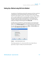
Setting Up a Method using Edit Entire Method
1260 Infinity Binary LC - System User Guide
111
5
Contents
6
1260 Infinity Binary LC - System User Guide
1260 Infinity Binary LC - System User Guide
1
The Agilent 1260 Infinity Binary LC Product Description
Features of the Agilent 1260 Infinity Binary LC
8
System Components 10
1260 Infinity Binary Pump (G1312B) 11
1260 Infinity High Performance Degasser (G4225A) 14
1260 Infinity High Performance Autosampler (G1367E) 15
1290 Infinity Thermostatted Column Compartment (G1316C)
1260 Infinity Diode Array Detector (G4212B) 19
1200 Infinity Series Quick Change Valves 21
Specifications
17
22
This chapter discusses the features of the 1260 Infinity Binary LC.
Agilent Technologies
7
1
The Agilent 1260 Infinity Binary LC - Product Description
Features of the Agilent 1260 Infinity Binary LC
Features of the Agilent 1260 Infinity Binary LC
The design concept of the 1260 Infinity Binary LC is to provide a liquid
chromatograph offering ultra fast and high resolution separation capability
and yet which retains full functionality for standard HPLC applications.
Therefore, it provides full backwards compatibility for your established HPLC
and UHPLC methods. The use of sub-two micron (STM) particles means that
for high flowrates or long columns additional pressure is required to drive the
mobile phase through the column. The flowpath of the 1260 Infinity Binary LC
is optimized to produce minimal backpressure, and ZORBAX RRHT columns
have an engineered particle size distribution that produces significantly less
backpressure than other STM columns.
The design features and benefits of the Agilent 1260 Infinity Binary LC are:
• The configurable delay volume down to 120 μL in the 1260 Infinity Binary
Pump combined with a flow range from 0.05 up to 5 mL/min at pressures
up to 600 bar provides universal applicability from narrow bore (2.1 mm
ID) to standard bore (4.6 mm ID) columns, matching the needs for both LC
and LC/MS.
• The standard delay volume configuration of the 1260 Infinity Binary Pump
allows you to run not only UHPLC but also conventional HPLC methods
without compromising performance or changing chromatographic patterns.
• The next generation flow-through design of the 1260 Infinity High
Performance Autosampler achieves highest precision for a wide range of
injection volumes (from 0.1 up to 100 μL) without changing sample loops.
It is designed for high sample throughput, low carryover, and fast injection
cycles.
• High temperature, up to 100 °C on certain columns, allows more selectivity
flexibility and reduces solvent viscosity to allow even faster separation.
• In the 1290 Infinity Thermostatted Column Compartment, different heater
(1.6 μL) and cooling elements (1.5 μL) for low extra-column volume can be
installed. The temperature is adjustable from 10 °C below ambient up to
100 °C.
8
1260 Infinity Binary LC - System User Guide
The Agilent 1260 Infinity Binary LC - Product Description
Features of the Agilent 1260 Infinity Binary LC
1
• The new pull-out valve drive design and user-exchangeable Quick-Change
valves in the 1290 Infinity Thermostatted Column Compartment boosts
usability and paves the way for ultra high-throughput, multi-method and
automated method development solutions.
• A low dispersion tubing kit and low volume flow cells minimize peak
dispersion for narrow bore columns.
• Baseline robustness and fast spectral acquisition at data rates up to 80 Hz
through the new optical design of the 1260 Infinity Diode Array Detector.
• Different UV detector flow cells for use with 2.1 , 3.0 and 4.6 mm inner
diameter columns are available, including the revolutionary Agilent
Max-Light cartridge flow cell with 60 mm optical path length (typical noise:
<±0.6 μAU/cm) for ultra sensitivity in detection.
A stepwise upgrade from 1100 Series or 1200 Series to Agilent 1260 Infinity
Binary LC is possible; for example a 1100 Series Detector or 1200 Series
Column Compartment can be further used in combination with a 1260 Infinity
Binary Pump.
1260 Infinity Binary LC - System User Guide
9
1
The Agilent 1260 Infinity Binary LC - Product Description
System Components
System Components
Numerous system configurations of the 1260 Infinity Binary LC are possible,
tailored to the needs of your individual application requirements. A few
configurations are described in more detail in this manual (see “System Setup
and Installation” on page 67). The modules that are described in the following
sections are typical components of a 1260 Infinity Binary LC. In addition to
these core components, individual solutions are available for specific
applications (some of which are described in the Chapter "Optimization").
10
1260 Infinity Binary LC - System User Guide
1
The Agilent 1260 Infinity Binary LC - Product Description
System Components
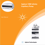
1260 Infinity Binary Pump (G1312B)
The binary pump comprises two identical pumps integrated into one housing.
Binary gradients are created by high-pressure mixing. Pulse damper and
mixer can be bypassed for low flowrate applications or whenever a minimal
transient volume is desirable. Typical applications are high throughput
methods with fast gradients on high resolution 2.1 mm columns. The pump is
capable of delivering flow in the range of 0.1 – 5 mL/min against up to 600 bar.
A solvent selection valve (optional) allows to form binary mixtures (isocratic
or gradient) from one of two solvents per channel. Active seal wash (optional)
is available for use with concentrated buffer solutions.
Principle of operation
The binary pump is based on a two-channel, dual-piston in-series design
which comprises all essential functions that a solvent delivery system has to
fulfill. Metering of solvent and delivery to the high-pressure side are
performed by two pump assemblies which can generate pressure up to
600 bar.
Each channel comprises a pump assembly including pump drive, pump head,
active inlet valve with replaceable cartridge, and outlet valve. The two
channels are fed into a low-volume mixing chamber which is connected via a
restriction capillary coil to a damping unit and a mixer. A pressure sensor
monitors the pump pressure. A purge valve with integrated PTFE frit is fitted
to the pump outlet for convenient priming of the pumping system.
1260 Infinity Binary LC - System User Guide
11
1
The Agilent 1260 Infinity Binary LC - Product Description
System Components
Ejg\ZkVakZ
B^mZg
9VbeZg
EjbedjiaZi
EgZhhjgZ
hZchdg
idlVhiZ
DjiaZi
kVakZ
>caZikVakZ
[gdb
hdakZci
WdiiaZ6
>caZikVakZ
B^m^c\
8]VbWZg
HZVah
E^hidch
Ejbe]ZVY6
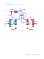
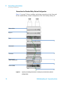
Figure 1
12
DjiaZi
kVakZ
HZVah
[gdb
hdakZci
WdiiaZ7
E^hidch
Ejbe]ZVY7
The Hydraulic Path of the Binary Pump with Damper and Mixer
1260 Infinity Binary LC - System User Guide
The Agilent 1260 Infinity Binary LC - Product Description
System Components
1
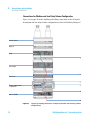
Damper and mixer can be bypassed for lowest delay volume of the binary
pump. This configuration is recommended for low flow rate applications with
steep gradients.
Figure 2 on page 13 illustrates the flow path in low delay volume mode. For
instructions on how to change between the two configurations, see the G1312B
Binary Pump User Manual.
NOTE
Bypassing the mixer while the damper remains in line is not a supported configuration and
may lead to undesired behavior of the binary pump.
B^mZg
9VbeZg
Ejg\ZkVakZ
EjbedjiaZi
EgZhhjgZ
hZchdg
idlVhiZ
DjiaZikVakZ
DjiaZi
kVakZ
>caZi
kVakZ
[gdbhdakZci
WdiiaZ6
>caZikVakZ
B^m^c\X]VbWZg
HZVah
HZVah
E^hidch
E^hidch
Ejbe]ZVY6
Figure 2
[gdbhdakZci
WdiiaZ7
Ejbe]ZVY7
The Hydraulic Path of the Binary Pump with Bypassed Damper and Mixer
1260 Infinity Binary LC - System User Guide
13
1
The Agilent 1260 Infinity Binary LC - Product Description
System Components
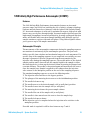
1260 Infinity High Performance Degasser (G4225A)
The Agilent 1260 Infinity High Performance Degasser, model G4225A,
comprises four separate vacuum chambers with semipermeable tubings, a
vacuum pump and control assembly. When the vacuum degasser is switched
on, the control assembly turns on the vacuum pump, which generates a low
pressure in the vacuum chambers. The pressure is measured by a pressure
sensor. The vacuum degasser maintains the low pressure by a controlled leak
in the air inlet filter and a regulation of the vacuum pump using the pressure
sensor.
The LC pump draws the solvents from their bottles through the
semipermeable tubes of the vacuum chambers. When solvents pass through
the vacuum chambers any dissolved gas in the solvents permeates through the
tubings into the vacuum chambers. The solvents will be degassed when leaving
the outlets of the vacuum degasser.
J=EA8
Ejbe
HZchdg
8dcigda
X^gXj^i
KVXjjb
ejbe
)hZeVgViZkVXjjbX]VbWZgh
HdakZci
KVXjjbXdciV^cZg
Figure 3
14
Overview (only one of the four solvent channels is shown)
1260 Infinity Binary LC - System User Guide
The Agilent 1260 Infinity Binary LC - Product Description
System Components
1
1260 Infinity High Performance Autosampler (G1367E)
Features
The 1260 Infinity High Performance Autosampler features an increased
pressure range (up to 600 bar) enabling the use of today’s column technology
(sub-two-micron narrow bore columns) with the Agilent 1260 Infinity Binary
LC. Increased robustness is achieved by optimized new parts, high speed with
lowest carry-over by flow through design, increased sample injection speed for
high sample throughput, increased productivity by using overlapped injection
mode, and flexible and convenient sample handling with different types of
sample containers, such as vials and well plates. Using 384-well plates allows
you to process up to 768 samples unattended.
Autosampler Principle
The movements of the autosampler components during the sampling sequence
are monitored continuously by the autosampler processor. The processor
defines specific time windows and mechanical ranges for each movement. If a
specific step of the sampling sequence is not completed successfully, an error
message is generated. Solvent is bypassed from the autosampler by the
injection valve during the sampling sequence. The needle moves to the desired
sample position and is lowered into the sample liquid in the sample to allow
the metering device to draw up the desired volume by moving its plunger back
a certain distance. The needle is then raised again and moved onto the seat to
close the sample loop. Sample is applied to the column when the injection
valve returns to the mainpass position at the end of the sampling sequence.
The standard sampling sequence occurs in the following order:
1 The injection valve switches to the bypass position.
2 The plunger of the metering device moves to the initialization position.
3 The needle lock moves up.
4 The needle moves to the desired sample vial (or well plate) position.
5 The needle lowers into the sample vial (or well plate).
6 The metering device draws the preset sample volume.
7 The needle lifts out of the sample vial (or well plate).
8 The needle is then moved onto the seat to close the sample loop.
9 The needle lock moves down.
10 The injection cycle is completed when the injection valve switches to the
mainpass position.
If needle wash is required it will be done between step 7 and 8.
1260 Infinity Binary LC - System User Guide
15
1
The Agilent 1260 Infinity Binary LC - Product Description
System Components
Injection Sequence
Before the start of the injection sequence, and during an analysis, the injection
valve is in the mainpass position. In this position, the mobile phase flows
through the autosampler metering device, sample loop, and needle, ensuring
all parts in contact with sample are flushed during the run, thus minimizing
carry-over.
When the sampling sequence begins, the valve unit switches to the bypass
position. Solvent from the pump enters the valve unit at port 1, and flows
directly to the column through port 6.
The final step of the sampling sequence is the inject-and-run step. The six-port
valve is switched to the main-pass position, and directs the flow back through
the sample loop, which now contains a certain amount of sample. The solvent
flow transports the sample onto the column, and separation begins. This is the
beginning of a run within an analysis. In this stage, all major
performance-influencing hardware is flushed internally by the solvent flow.
For standard applications, no additional flushing procedure is required.
Flush the Needle
Before injection and to reduce the carry-over for very sensitive analysis, the
outside of the needle can be washed in a flush port that is located behind the
injector port on the sampling unit. As soon as the needle is on the flush port a
peristaltic pump delivers some solvent during a defined time to clean the
outside of the needle. At the end of this process the needle returns to the
injection port.
16
1260 Infinity Binary LC - System User Guide
The Agilent 1260 Infinity Binary LC - Product Description
System Components
1
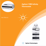
1290 Infinity Thermostatted Column Compartment (G1316C)
The Agilent 1290 Infinity Thermostatted Column Compartment (TCC) controls
the temperature between 10 °C below ambient and up to 100 °C at 2.5 ml/min
and 80 °C at up to 5 ml/min, respectively. The temperature stability
specification is ±0.05 °C and the accuracy specification ±0.5 °C (with
calibration)1. This is achieved by a combination of conduction from contact
with the thermostat vanes, still-air temperature in the column environment
and most importantly by pre-heating (or cooling) the mobile phase by passing
it through a heat exchanger before entering the column. There are two
independent temperature zones in each TCC which can work together for long
columns up to 300 mm length or work at different temperatures for short
columns of 100 mm length or less.
The module comes with a 1.6 μl low dispersion heat exchanger and each valve
kit contains additional low dispersion heat exchangers for each column. The
low dispersion heat exchangers, up to 4, can be mounted flexibly inside the
TCC. For conventional HPLC operation, 3 μl and 6 μl built-in heat exchangers
are also available.
Each TCC can accommodate one internal valve drive to facilitate valve
switching applications from simple switching between two columns to
alternating column regeneration, sample preparation or column back-flushing.
Each valve head comes as a complete kit containing all required capillaries,
additional low dispersion heat exchangers and other parts.
The switching valves have exceptional ease-of-use and flexibility when making
connections to the valve: When pressed, the drive unit of the Quick Change
Valve slides forward for easy access (see Figure 4 on page 18 left). Alternative
valve heads can be interchanged by the user on the drive mechanism for
different applications (see Figure 4 on page 18 right). Note the RFID tag on top
of the valve head.
1
All specifications are valid for distilled water at ambient temperature of 25 °C, setpoint at 40 °C
and a flow range from 0.2 to 5 ml/min.
1260 Infinity Binary LC - System User Guide
17
1
The Agilent 1260 Infinity Binary LC - Product Description
System Components
Figure 4
Quick change valve in TCC
Up to three TCC can be “clustered” to allow advanced applications such as
switching between eight columns for automated method development or to
make additional columns available for different applications. Thus, the column
to be used becomes a simple method parameter. This requires two 8 position/9
port valve heads, one each in two of the TCCs. Clustered TCC are represented
by the software as one unit with one interface for ease of operation.
Further improvements compared to earlier designs include better thermal
insulation, better capillary guides and a “door open” sensor so that methods
can define that the door must be closed – especially useful for low or
high-temperature methods.
18
1260 Infinity Binary LC - System User Guide
The Agilent 1260 Infinity Binary LC - Product Description
System Components
1
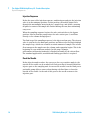
1260 Infinity Diode Array Detector (G4212B)
The 1260 Infinity Diode-Array Detector (DAD) is a new optical design using a
cartridge cell with optofluidic waveguide technology, offering high sensitivity
with low dispersion, a wide linear range, and a very stable baseline for
standard or ultra-fast LC applications. The Agilent Max-Light cartridge cell
dramatically increases the light transmission by utilizing the principle of total
internal reflection along a non-coated fused silica capillary, achieving a new
level of sensitivity without sacrificing resolution through cell volume
dispersion effects. This design minimizes baseline perturbations that are
caused by refractive index or thermal effects and results in more reliable
integration of peak areas.
B^ggdg
<gVi^c\
Deid[aj^Y^XlVkZ\j^YZ
9ZjiZg^jbaVbe
BVm"a^\]iXVgig^Y\ZXZaa
Ha^i
&%')ZaZbZciY^dYZ"VggVn
Figure 5
The light path through the DAD
The module also incorporates electronic temperature control to further
enhance the resistance to ambient temperature effects. Although the hydraulic
volume of the Max-Light cartridge cell is very small, the path length is a
standard 10 mm. However, for even higher sensitivity the alternative Agilent
Max-Light high sensitivity cell is available with a path length of 60 mm. Cells
are easily exchanged by sliding them in or out of the cell holder and they are
auto-aligned in the optical bench. The DAD light source is a deuterium lamp
and the operating wavelength range that is covered is 190 to 640 nm. This is
detected by a diode-array comprising 1024 diodes. The entrance to the
spectrograph is through a fixed optical slit of 4 nm.
1260 Infinity Binary LC - System User Guide
19
1
The Agilent 1260 Infinity Binary LC - Product Description
System Components
The chromatographic signals are extracted from the diode-array data within
the firmware of the module. Up to eight individual signals can be defined.
Each of them comprises a signal wavelength, a diode-bunching bandwidth and
- if required - a reference wavelength and bandwidth. Signals can be output at
80 Hz (80 data points/second) for accurate recording of the fastest
(narrowest) chromatographic peaks. At the same time, the module can also
output full-range spectra to the data system at the same rate of 80 Hz.
For regulated laboratories, it is important that all the method parameters are
recorded. The 1260 Infinity DAD not only records the instrument setpoints but
also has RFID tags (radio-frequency identification tags) incorporated into the
lamp and flow cell cartridge so that the identity and variables of these
important components are also recorded by the system.
20
1260 Infinity Binary LC - System User Guide
The Agilent 1260 Infinity Binary LC - Product Description
System Components
1
1200 Infinity Series Quick Change Valves
Agilent 1200 Infinity Quick Change Valves support a variety of challenging
valve applications. Each valve head comes as a complete kit containing all
required capillaries, additional low dispersion heat exchangers and other
parts.
Some typical applications for Quick Change Valves are:
• Dual column selection
• Sample enrichment
• Sample clean-up
• Alternating column regeneration
• Special applications, such as method development or 2D-LC
For detailed descriptions of these applications, please refer to the Valve
Solution User Guide.
1260 Infinity Binary LC - System User Guide
21
1
The Agilent 1260 Infinity Binary LC - Product Description
Specifications
Specifications
The modular design of the 1260 Infinity Binary LC allows you to configure a
system that exactly meets your individual application requirements. This
individual configuration can be different from the standard configuration
which is described in this System User Guide.
The physical and performance specifications of the 1260 Infinity Binary Pump
are shown below. Information on the specifications of other modules in your
system can be found in the respective module user manuals.
22
1260 Infinity Binary LC - System User Guide
1
The Agilent 1260 Infinity Binary LC - Product Description
Specifications
Physical Specifications 1260 Infinity Binary Pump (G1312B)
Table 1
Physical Specifications
Type
Specification
Weight
15.5 kg (34 lbs)
Dimensions
(height × width × depth)
180 x 345 x 435 mm
(7 x 13.5 x 17 inches)
Line voltage
100 – 240 VAC, ± 10 %
Line frequency
50 or 60 Hz, ± 5 %
Power consumption
220 VA, 74 W / 253 BTU
Ambient operating
temperature
4–55 °C (39–131 °F)
Ambient non-operating
temperature
-40 – 70 °C (-40 – 158 °F)
Humidity
< 95 % r.h. at 40 °C (104 °F)
Operating altitude
Up to 2000 m (6562 ft)
Non-operating altitude
Up to 4600 m (15091 ft)
For storing the module
Safety standards:
IEC, CSA, UL
Installation category II, Pollution degree 2
For indoor use only.
1260 Infinity Binary LC - System User Guide
Comments
Wide-ranging
capability
Maximum
Non-condensing
23
1
The Agilent 1260 Infinity Binary LC - Product Description
Specifications
Performance Specifications
Table 2
24
Performance Specifications of the Agilent 1260 Infinity Binary Pump (G1312B)
Type
Specification
Comments
Hydraulic system
Two dual piston in series pumps with
servo-controlled variable stroke drive,
power transmission by gears and ball
screws, floating pistons
Setable flow range
Set points 0.001 – 5 mL/min, in
0.001 mL/min increments
Flow range
0.05 – 5.0 mL/min
Flow precision
≤0.07 % RSD or ≤0.02 min SD, whatever is
greater
based on retention time at
constant room temperature
Flow accuracy
± 1 % or 10 µL/min, what ever is greater
pumping degassed H2O at
10 MPa (100 bar)
Pressure operating
range
Operating range 0 – 60 MPa (0 – 600 bar,
0 – 8700 psi) up to 5 mL/min
Pressure pulsation
< 2 % amplitude (typically < 1.3 %), or
< 0.3 MPa (3 bar), whatever is greater, at
1 mL/min isopropanol, at all pressures
> 1 MPa (10 bar, 147 psi)
Low delay volume configuration:
< 5 % amplitude (typically < 2 %)
Compressibility
compensation
Pre-defined, based on mobile phase
compressibility
Recommended pH
range
1.0 – 12.5 , solvents with pH < 2.3 should
not contain acids which attack stainless
steel
Gradient formation
High-pressure binary mixing
Delay volume
Standard delay volume configuration:
600 – 800 µL, (includes 400 µL mixer),
dependent on back pressure
Low delay volume configuration:
120 µL
Composition range
settable range: 0 – 100 %
recommended range: 1 – 99 % or
5 µL/min per channel, whatever is greater
measured with water at
1 mL/min (water/caffeine
tracer)
1260 Infinity Binary LC - System User Guide
1
The Agilent 1260 Infinity Binary LC - Product Description
Specifications
Table 2
NOTE
Performance Specifications of the Agilent 1260 Infinity Binary Pump (G1312B)
Type
Specification
Comments
Composition
precision
< 0.15 % RSD or < 0.04 min SD whatever
is greater
at 0.2 and 1 mL/min; based
on retention time at constant
room temperature
Composition
accuracy
± 0.35 % absolute, at 2 mL/min, at
10 MPa (100 bar)
(water/caffeine tracer)
Control
Agilent control software (e.g.
ChemStation, EZChrom, OL, MassHunter)
Local control
Agilent Instant Pilot
Analog output
For pressure monitoring, 1.33 mV/bar,
one output
Communications
Controller-area network (CAN), RS-232C,
APG Remote: ready, start, stop and
shut-down signals, LAN optional
Safety and
maintenance
Extensive support for troubleshooting and
maintenance is provided by the Instant
Pilot, Agilent Lab Advisor, and the
Chromatography Data System.
Safety-related features are leak detection,
safe leak handling, leak output signal for
shutdown of pumping system, and low
voltages in major maintenance areas.
GLP features
Early maintenance feedback (EMF) for
continuous tracking of instrument usage
in terms of seal wear and volume of
pumped mobile phase with pre-defined
and user settable limits and feedback
messages. Electronic records of
maintenance and errors
Housing
All materials are recyclable
Revision B.02.00 or above
For use with flow rates below 500 µl/min or for use without damper and mixer a vacuum
degasser is required.
All specification measurements are done with degassed solvents.
1260 Infinity Binary LC - System User Guide
25
1
26
The Agilent 1260 Infinity Binary LC - Product Description
Specifications
1260 Infinity Binary LC - System User Guide
1260 Infinity Binary LC - System User Guide
2
Introduction
Theory of Using Smaller Particles in Liquid Chromatography
Benefits of small particle size columns
Frictional Heating
28
34
37
This chapter gives an introduction to the Agilent 1260 Infinity Binary LC and the
underlying concepts.
Agilent Technologies
27
2
Introduction
Theory of Using Smaller Particles in Liquid Chromatography
Theory of Using Smaller Particles in Liquid Chromatography
Introduction
In 2003, Agilent introduced the first commercially available, totally porous
silica columns with 1.8 μm particles.
In combination with the Agilent 1260 Infinity Binary LC the sub-two micron
(1.8 μm) particle size columns can be used in pursuit of two main objectives:
1 Faster Chromatography
Short columns with sub-two-micron particles offer the opportunity to
dramatically reduce analysis time by increasing the flow rate without losing
separation performance.
2 Higher Resolution
Long columns with sub-two-micron particles provide higher efficiency and
therefore higher resolution, which is required for the separation of complex
samples.
The pressure that is needed to drive solvent through a column containing STM
(sub-two micron) particles rises rapidly as flow rate is increased for faster
separations and very rapidly as the length of the column increases for more
resolution. Thus the acceptance of STM columns has been synonymous with
the development of UHPLC systems – that is HPLC systems offering higher
pressures than the 400 bar norm that was extant since the early days of HPLC.
Today, Agilent offers the 1290 Infinity LC for highest UHPLC requirements
with pressures up to 1200 bar.
28
1260 Infinity Binary LC - System User Guide
Introduction
Theory of Using Smaller Particles in Liquid Chromatography
2
The Theory
I]ZdgZi^XVaEaViZ=Z^\]i=
Separation efficiency in HPLC can be described by the van Deemter equation
(Figure 6 on page 29). This results from the plate-height model that is used to
measure the dispersion of analytes as they move down the column. H is the
Height Equivalent to a Theoretical Plate (sometimes HETP), dp is the particle
size of the column packing material, u0 is the linear velocity of the mobile
phase and A, B and C are constants that are related to the different dispersive
forces. The A term relates to eddy diffusion or multiple flow paths through the
column; B relates to molecular diffusion along the column axis (longitudinal);
C relates to mass transfer of the analyte between the mobile and stationary
phases. The separation is at its most efficient when H is at a minimum. The
effect of each individual term and the combined equation are shown in
Figure 6 on page 29where the plate height is plotted against the linear flow
rate through the column. This type of plot is known as a Van Deemter Curve
and is used to determine the optimum flow rate (minimum point of the curve)
for best efficiency of separation for a column.
aVg\ZeVgi^XaZ
hbVaaeVgi^XaZ
GZhjai^c\KVc"9ZZbiZgXjgkZ
GZh^hiVcXZidBVhhIgVch[Zg
Bjai^eVi]IZgb!
:YYn9^[[jh^dc
Adc\^ijY^cVaY^[[jh^dc
Figure 6
A^cZVg[adlj
A hypothetical Van Deemter curve
1260 Infinity Binary LC - System User Guide
29
2
Introduction
Theory of Using Smaller Particles in Liquid Chromatography
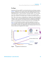
The van Deemter plots in Figure 7 on page 30 show that reducing particle size
increases efficiency. Switching from commonly used 3.5 μm and 5.0 μm
particle sizes to 1.8 μm particles offers significant performance improvements.
The 1.8 μm particles give two to three times lower plate height values and
proportionately higher efficiencies. This allows a shorter column to be used
without sacrificing resolution and hence the analysis time is also reduced by a
factor of two to three. The increased efficiency is derived to a large extent
from the reduction in multiple flow paths as a result of the smaller particles this leads to a smaller A term (eddy diffusion). In addition, smaller particles
mean shorter mass transfer times, reducing the C term, and it can be seen that
the overall effect is a much reduced loss of efficiency as the flow rate increases
(the slope of the line is reduced). This means that the separation on smaller
particles can be further accelerated by increasing the flow rates without
significantly reducing efficiency.
%#%%)*
%#%%)%
=:IEXb$eaViZ
%#%%(*
%#%%(%
%#%%'*
*#%¥b
%#%%'%
%#%%&*
(#*¥b
%#%%&%
&#-¥b
%#%%%*
%#%%%%
*#%ba$b^c
'ba$b^c
"%#%%%*
%#%
%#'
%#)
%#+
%#-
&#%
&#'
&#)
&#+
>ciZghi^i^Vaa^cZVgkZadX^in¥"Xb$hZX
Z
Figure 7
30
Van Deemter curve for different particle sizes
1260 Infinity Binary LC - System User Guide
Introduction
Theory of Using Smaller Particles in Liquid Chromatography
2
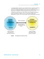
A chromatographic separation can be optimized based on physical parameters
of the HPLC column such as particle size, pore size, morphology of the
particles, the length and diameter of the column, the solvent velocity, and the
temperature. In addition, the thermodynamics of a separation can be
considered and the properties of the solute and the stationary and mobile
phases (percentage of organic solvent, ion strength, and pH) can be
manipulated to achieve the shortest possible retention and highest selectivity.
DEI>B>O:
@>C:I>8H
d[H:E6G6I>DC
Hadl6Y"dg9Zhdgei^dc
DEI>B>O:
I=:GBD9NC6B>8H
d[H:E6G6I>DC
Cdc"a^cZVg^hdi]Zgbh
8]Zb^XVa:fj^a^Wgjbe=
EgZhhjgZ
E=NH>8H
8=:B>HIGN
EVgi^XaZH^oZ!Edgdh^in!
8dajbc9^bZch^dch!
;adlKZadX^in!IZbeZgVijgZ
HiVi^dcVgnVcYBdW^aZ
E]VhZEgdeZgi^Zh!HdajiZ
EgdeZgi^Zh!IZbeZgVijgZ
Figure 8
Selecting optimal conditions for HPLC
1260 Infinity Binary LC - System User Guide
31
2
Introduction
Theory of Using Smaller Particles in Liquid Chromatography
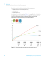
Resolution can be described as a function of three parameters:
• column efficiency or theoretical plates (N),
• selectivity (α),
• retention factor (k).
According to the resolution equation ( Figure 9 on page 32 ), the selectivity has
the biggest impact on resolution (Figure 10 on page 32). This means that the
selection of appropriate mobile and stationary phase properties and
temperature is critical in achieving a successful separation.
32
Figure 9
Resolution equation
Figure 10
Effect of plate number, separation factor and retention factor on R
1260 Infinity Binary LC - System User Guide
Introduction
Theory of Using Smaller Particles in Liquid Chromatography
2
No matter whether the UHPLC separation method is being newly developed or
simply transferred from an existing conventional method, it is clearly
beneficial to have a wide choice of stationary phase chemistries available in a
range of column formats.
Agilent offers more than 140 ZORBAX 1.8 μm Rapid Resolution High
Throughput (RRHT) columns (14 selectivity choices; 15 to 150 mm long; 2.1 ,
3.0 and 4.6 mm internal diameters).
Additionally to the ZORBAX columns, PoroShell columns with nine selectivity
choices are available for use with the Agilent 1260 Infinity Binary LC.
This enables the optimum stationary phase to be selected so that the
selectivity is maximized. The resolution, flow rate, and analysis time can be
optimized by selecting the appropriate column length and diameter and
operation with longer STM columns has become more accessible than ever
before.
PoroShell columns are so-called superficially porous particle (SPP) columns.
In contrast to totally porous silica columns, these SPP columns have a solid
core (1.7 μm in diameter) and a porous silica layer (0.5 μm thickness)
surrounding it. Speed and resolution of PoroShell columns are comparable to
sub-two micron columns with up to 50 % less backpressure. PoroShell columns
have enjoyed a recent resurgence in smaller particle sizes than the older
'pellicular' particle columns. The current interest in this technology is driven
by its re-introduction in smaller particle sizes, such as the sub 3 micron sizes,
for use in typical small molecule reversed phase separations.
Many laboratories perform an extensive screening process to select the best
combination of stationary phase, mobile phase, and temperature for their
separations. The Agilent 1200 Infinity Series Multi-Method Development
Solution facilitates complete automation of this time-consuming selection
process – making method development and method transfer an easy and
reliable task.
ZORBAX 1.8 μm RRHT columns use the same chemistry as ZORBAX columns
with 3.5 and 5 μm particles. As a result, for any particular ZORBAX phase, the
5.0 , 3.5 and 1.8 μm particles provide identical selectivity, which allows easy,
fast, and secure bidirectional method transfer between conventional LC and
UHPLC.
1260 Infinity Binary LC - System User Guide
33
2
Introduction
Benefits of small particle size columns
Benefits of small particle size columns
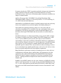
Faster Chromatography
There are several advantages of having shorter run times. High Throughput
labs now have higher capacity and can analyze more samples in less time.
More samples in less time also means lower costs. For example, by reducing
the analysis time from 20 min per sample to 5 min, the cost for 700 samples is
reduced by 79 % (Table 3 on page 34).
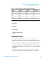
Table 3
Time and cost savings over 700 runs
Cycle time
20 min cycle time
5 min cycle time
Runs
700
700
Approx. costs/analysis1
$ 10.58
$ 2.24
Approx. cost/700runs1
$ 7400
$ 1570
Cost savings
-
$ 5830
Time2
10 days
2.5 days
1
solvents = $ 27/l, disposal = $ 2/l, labor = $ 30/h
2
24 hours/day
The Agilent cost savings calculator provides an easy way to calculate the cost
savings by switching from conventional HPLC to UHPLC using 1.8 μm particle
size columns. This calculator is available on the Agilent Technologies web site
along with a method translator calculator – www.chem.agilent.com. The
results are presented graphically and in tabular form.
Shorter run times also deliver faster answers. This is important in process
control and rapid release testing. Instead of waiting hours to release a single
batch of a drug, all the system suitability, calibration and sample analysis can
now be done in less than an hour. Rapid answers are also important for
synthetic chemists using open access LC/MS systems for compound
confirmation and reaction control. Shorter run times can also accelerate the
method development process significantly.
34
1260 Infinity Binary LC - System User Guide
Introduction
Benefits of small particle size columns
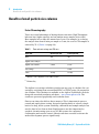
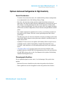
8dajbc
AZc\i]
bb
8dajbc
:[[^X^ZcXn
C*¥b
8dajbc
:[[^X^ZcXn
C(#*¥b
8dajbc
:[[^X^ZcXn
C&#-¥b
&*%
&'!*%%
'&!%%%
(*!%%%
&%%
-!*%%
&)!%%%
'(!'*%
,*
+%%%
&%!*%%
&,!*%%
,!%%%
&'!%%%
2
6cVanh^h
I^bZ
GZYjXi^dc
:[[^X^ZcXn
6cVanh^h
C
I^bZ
"((
"*%
EgZhhjgZ
*%
)!'%%
EZV`
"+,
KdajbZ
(%
C#6#
)!'%%
+!*%%
HdakZci
"-%
JhV\Z
&*
C#6#
Figure 11
'!&%%
'!*%%
".%
Relation between particle size, efficiency and analysis time
Analysis time can be shortened without sacrificing column efficiency by
optimizing particle size and pressure.
1260 Infinity Binary LC - System User Guide
35
2
Introduction
Benefits of small particle size columns
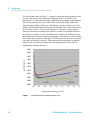
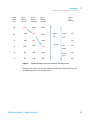
Higher Resolution
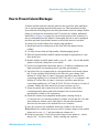
6WhdgWVcXZPb6JR
Long columns packed with smaller particles result in higher efficiency and
higher resolution. This is important for analysis of complex samples from
metabolomics or proteomics studies. Also, applications such as impurity
profiling can benefit from higher separation power. Even the LC/MS analysis
of drugs in biological fluids can benefit from the higher peak capacity, because
of the reduced interference from ion suppression. In general, higher
separation power provides more confidence in the analytical results.
EZV`XVeVX^in2+.)
A8l^i]<8gZhdaji^dc
I^bZPb^cR
Figure 12
36
Peak capacities of more than 700 can be achieved using a ZORBAX RRHT
SB-C18 column (2.1 x 150 mm, 1.8 µm) to analyze a tryptic digest of BSA
1260 Infinity Binary LC - System User Guide
2
Introduction
Frictional Heating
Frictional Heating
Forcing mobile phase through the column at higher pressure and higher flow
rates generates heat. The resulting temperature gradients (radial and
longitudinal) can have an impact on the column efficiency.
where F is the flow rate and p is the pressure.
Powerful column thermostatting (for example, using a water bath) generates a
strong radial temperature gradient, which leads to significant loss in column
efficiency. Still-air column thermostatting reduces the radial temperature
gradient and therefore reduces the efficiency losses, but a higher column
outlet temperature has to be accepted. The raised temperature may have an
effect on selectivity. At lower back-pressure, performance losses due to
frictional heat are minimized so that 4.6 or 3 mm inner diameter
sub-2-micron columns still deliver superior efficiencies compared with the
respective 2.1 mm inner diameter columns.
In summary, the use of sub-two-micron packing material offers benefits of
increased efficiency, higher resolution and faster separations.
The features of the Agilent 1260 Infinity Binary LC are discussed in the
chapter Product Description. The chapter Optimization considers how to
apply the theory and use these features to develop optimized separations.
1260 Infinity Binary LC - System User Guide
37
2
38
Introduction
Frictional Heating
1260 Infinity Binary LC - System User Guide
1260 Infinity Binary LC - System User Guide
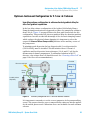
3
Optimization of the Agilent 1260 Infinity
Binary LC
How to Configure the Optimum Delay Volume 40
Delay Volume and Extra-Column Volume 40
Delay Volumes in the Agilent 1260 Infinity Binary LC 42
Optimum Instrument Configuration for 2.1 mm i.d. Columns 43
Optimum Instrument Configuration for 3 and 4.6 mm i.d. Columns
How to Achieve Higher Injection Volumes
45
47
How to Achieve Shorter Cycle Times 48
How to Achieve High Throughput 50
How to Achieve Lowest Carry-over
51
How to Achieve Higher Resolution 53
Optimum Instrument Configuration for High Resolution
How to Achieve Higher Sensitivity 60
Optimum Instrument Configuration for High Sensitivity
Choosing a Flow Cell 63
How to Prevent Column Blockages
56
61
65
This chapter considers how to apply the theory and use the features of the LC
system to develop optimized separations.
Agilent Technologies
39
3
Optimization of the Agilent 1260 Infinity Binary LC
How to Configure the Optimum Delay Volume
How to Configure the Optimum Delay Volume
Delay Volume and Extra-Column Volume
The delay volume is defined as the system volume between the point of mixing
in the pump and the top of the column.
The extra-column volume is defined as the volume between the injection point
and the detection point, excluding the volume in the column.
Delay Volume
In gradient separations, this volume causes a delay between the mixture
changing in the pump and that change reaching the column. The delay
depends on the flow rate and the delay volume of the system. In effect, this
means that in every HPLC system there is an additional isocratic segment in
the gradient profile at the start of every run. Usually the gradient profile is
reported in terms of the mixture settings at the pump and the delay volume is
not quoted even though this will have an effect on the chromatography. This
effect becomes more significant at low flow rates and small column volumes
and can have a large impact on the transferability of gradient methods. It is
important, therefore, for fast gradient separations to have small delay
volumes, especially with narrow bore columns (that is, 2.1 mm i.d.) as often
used with mass spectrometric detection.
As an example, in HPLC methods using 5 μm packing material flow rates of
1 ml/min are typically used in a 4.6 mm i.d. column and about 0.2 ml/min in a
2.1 mm i.d column (same linear velocity in the column). On a system with a
typical delay volume of 1000 μl and using a 2.1 mm column, there would be an
initial “hidden” isocratic segment of 5 min whereas on a system with 600 μl
delay volume the delay would be 3 min. These delay volumes would be too high
for run times of one or two minutes. With sub-two μm packings, the optimum
flow rate (from the Van Deemter curve) is a little higher and so fast
chromatography can use three to five times these flow rates yielding delay
times of about one minute. However, the delay volume must be reduced
further to achieve delay times which are a fraction of the intended run time.
This is achieved with the Agilent 1260 Infinity Binary LC due to the low delay
volume of the pump flow path and low-volume of the flow path through the
autosampler.
40
1260 Infinity Binary LC - System User Guide
Optimization of the Agilent 1260 Infinity Binary LC
How to Configure the Optimum Delay Volume
3
Extra-Column Volume
Extra-column volume is a source of peak dispersion that will reduce the
resolution of the separation and so should be minimized. Smaller diameter
columns require proportionally smaller extra-column volumes to keep peak
dispersion at a minimum.
In a liquid chromatograph the extra-column volume will depend on the
connection tubing between the autosampler, column, and detector; and on the
volume of the flow cell in the detector. The extra-column volume is minimized
with the Agilent 1260 Infinity Binary LC due to the narrow-bore (0.12 mm i.d.)
tubing, the low-volume heat exchangers in the column compartment and the
Max-Light cartridge cell in the detector.
1260 Infinity Binary LC - System User Guide
41
3
Optimization of the Agilent 1260 Infinity Binary LC
How to Configure the Optimum Delay Volume
Delay Volumes in the Agilent 1260 Infinity Binary LC
Table 4 on page 42 and Table 5 on page 42show the component volumes which
contribute to system delay volume in the Agilent 1260 Infinity Binary LC
System.
Table 4
Delay volumes of the 1260 Infinity Binary LC modules
Components
Delay Volume (µL)
Binary Pump1
120
Binary Pump2
600 – 800
Low volume mixer
200
Mixer
400
Autosampler
270
Low dispersion heat exchanger
1.6
Built-in heat exchanger
3 and 6
1
in low delay volume configuration with bypassed damper and mixer
2
in standard delay volume configuration
Table 5
Delay volumes of 1260 Infinity Binary LC configurations
System Configuration
Delay Volume (µL)
Low delay volume configuration
Pump: 120
Autosampler:
Medium delay volume configuration
Pump: 320
Standard delay volume configuration
Pump: 600 – 800
Switching between configurations can be done in two ways:
• manually, by disconnecting and reconnecting capillaries
• automatically, using a 600 bar 2PS/6PT valve (optional)
42
1260 Infinity Binary LC - System User Guide
Optimization of the Agilent 1260 Infinity Binary LC
How to Configure the Optimum Delay Volume
3
Optimum Instrument Configuration for 2.1 mm i.d. Columns
Low delay volume configuration to achieve shortest gradient delay for
ultra-fast gradient separations
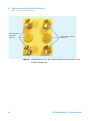
In the low delay volume configuration of the Agilent 1260 Infinity Binary
Pump the damper and mixer are bypassed to reduce the pump delay volume to
about 120 μL. Figure 13 on page 43shows the flow path connections for this
configuration. This provides the shortest gradient delay for ultra-fast gradient
separations. In order to take full advantage of the electronic damping control
which replaces the physical volume damping it is important to select the
respective Enhanced Solvent Compressibility function in the auxiliary screen of
the pump menu.
To minimize peak dispersion the low dispersion kit ( Low dispersion kit
(G1316-68744)) must be installed. This kit includes short 0.12 mm i.d.
capillaries and low dispersion heat exchangers (1.6 μL and 1.5 μL) for the
thermostatted column compartment. To maintain resolution in the UV
detector, a low volume flow cell should be used. See “Choosing a Flow Cell” on
page 63 for flow cell recommendations).
;adlEVi]
9^hXdccZXidcan]ZgZ
B^m^c\"I
EgZhhjgZ
HZchdg
EgZhhjgZ
HZchdg
Ejg\ZKVakZ
AdlYZaVnkdajbZ
&'%¥aYZaVn
6
Figure 13
7
Ejg\Z
KVakZ
Low delay configuration for 2.1 mm inner diameter columns
It is important to remember to set the correct parameter in the pump auxiliary
screen. This ensures that the correct compressibility values are always applied
for the mobile phases used. Calibration curves are available for most common
solvents.
1260 Infinity Binary LC - System User Guide
43
3
Optimization of the Agilent 1260 Infinity Binary LC
How to Configure the Optimum Delay Volume
Medium delay volume configuration to achieve highest UV sensitivity
For high sensitivity UV applications an additional 200 μL mixer ( Low volume
mixer ( 200 μL) (5067-1565)) can be installed to reduce any residual mixing
noise. This small mixer gives the lowest UV baseline noise even under extreme
gradient conditions. See Figure 14 on page 44.
BZY^jbYZaVnkdajbZ
('%¥a
[dgjaigV[VhiVcY
hjeZg^dgJKhZch^i^k^in
l^i]'#&bb>9
Xdajbch
'%%¥aB^mZg
+%%WVg9VbeZg
B^m^c\"I
EgZhhjgZ
HZchdg
EgZhhjgZ
HZchdg
'%%¥a
B^mZg
Ejg\Z
KVakZ
Figure 14
44
Medium delay volume configuration for 2.1 mm ID columns with highest UV
sensitivity
1260 Infinity Binary LC - System User Guide
3
Optimization of the Agilent 1260 Infinity Binary LC
How to Configure the Optimum Delay Volume
Optimum Instrument Configuration for 3 and 4.6 mm i.d. Columns
Standard delay volume configuration for highest UV sensitivity and direct
method transferability
The relative column volumes for 3 mm and 4.6 mm inner diameter columns
are about two and five times larger respectively than for the same length
2.1 mm i.d. columns, and the flow rates that are used are also proportionally
higher. Therefore, the standard delay volume of the binary pump will not
result in a significantly higher gradient delay.
;adlEVi]
9^hXdccZXidcan]ZgZ
)%%¥aB^mZg
B^m^c\"I
+%%WVg9VbeZg
EgZhhjgZ
HZchdg
EgZhhjgZHZchdg
HiYYZaVnkdajbZ
+%%"-%%¥a
Ejg\ZKVakZ
9VbeZg
7
6
)%%¥aB^mZg
Ejg\ZKVakZ
Figure 15
Standard delay volume configuration for 3 and 4.6 mm ID columns with
highest UV sensitivity
1260 Infinity Binary LC - System User Guide
45
3
Optimization of the Agilent 1260 Infinity Binary LC
How to Configure the Optimum Delay Volume
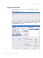
The standard delay volume configuration is also the configuration which
provides direct method transferability from the Agilent 1100 and 1200 Series
LC system to the 1260 Infinity Binary LC or vice versa. Figure Figure 16 on
page 46 shows two overlaid chromatograms of a method for analysis of
paracetamol and related impurities. The method was transferred from an
Agilent 1200 Series LC system to an Agilent 1260 Infinity Binary LC with the
chromatographic conditions (column, mobile phase, pump settings, injection
volume, column temperature, detector settings) left unchanged. As can be
seen, a seamless method transfer is possible.
Figure 16
46
Comparison Agilent 1200 Series and Agilent 1260 Infinity LC system on one
Configuration
1260 Infinity Binary LC - System User Guide
Optimization of the Agilent 1260 Infinity Binary LC
How to Achieve Higher Injection Volumes
3
How to Achieve Higher Injection Volumes
The standard configuration of the Agilent 1260 Infinity Autosampler can inject
a maximum volume of 100 μL with the standard loop capillary. To increase the
injection volume, the Multidraw upgrade kit (G1313-68711)can be installed.
With the kit, you can add a maximum of 400 μL or 1400 μL to the injection
volume of your injector. The total volume is then 500 μL or 1500 μL for the
1260 Infinity Autosampler with 100 μL analytical head. Note that the delay
volume of your autosampler is extended when using the extended seat
capillaries from the multi-draw kit. When calculating the delay volume of the
autosampler you have to double the volume of the extended capillaries. The
system delay volume due to the autosampler will increase accordingly.
Whenever a method is scaled down from a larger column to a smaller column
it is important that the method translation makes an allowance for reducing
the injection volume in proportion to the volume of the column to maintain
the performance of the method. This is to keep the volume of the injection at
the same percentage volume with respect to the column. This is particular
important if the injection solvent is stronger (more eluotropic) than the
starting mobile phase and any increase will affect the separation particularly
for early running peaks (low retention factor). In some cases, it is the cause of
peak distortion and the general rule is to keep the injection solvent the same
or weaker than the starting gradient composition. This has a bearing on
whether, or by how much, the injection volume can be increased and the user
should check for signs of increased dispersion (wider or more skewed peaks
and reduced peak resolution) in trying to increase the injection size. If an
injection is made in a weak solvent, then the volume can probably be increased
further because the effect will be to concentrate the analyte on the head of the
column at the start of the gradient. Conversely if the injection is in a stronger
solvent than the starting mobile phase then increased injection volume will
spread the band of analyte down the column ahead of the gradient resulting in
peak dispersion and loss of resolution.
Perhaps the main consideration in determining injection volume is the
diameter of the column as this will have a large impact on peak dispersion.
Peak heights can be higher on a narrow column than with a larger injection on
a wider column because there is less peak dispersion. With 2.1 mm i.d.
columns, typical injection volumes might range up to 5 to10 μl but it is very
dependent on the chemistry of the analyte and mobile phase as discussed
above. In a gradient separation, injection volumes of about 5 % of the column
volume might be achieved while maintaining good resolution and peak
dispersion.
1260 Infinity Binary LC - System User Guide
47
3
Optimization of the Agilent 1260 Infinity Binary LC
How to Achieve Shorter Cycle Times
How to Achieve Shorter Cycle Times
Shorter cycle times can be achieved by selecting a short column with good
selectivity. The column dimensions are also determined by the detection
system that is used. For UV detection, 3.0 mm inner diameter columns are
ideal, because here the highest linear velocities can be obtained. With 4.6 mm
inner diameter columns, high linear velocities can also be reached, but the
maximum flow rate is limited to 5 mL/min.
The pump should be used in its standard delay volume configuration (see
Figure 13 on page 43) for 4.6 mm inner diameter and 3.0 mm inner diameter
columns. For 2.1 mm inner diameter columns, the low delay volume
configuration should be used. In addition, when using 2.1 mm inner diameter
columns, the low dispersion kit should be installed to provide lowest
extra-column volume. For highest UV sensitivity, it is recommended in
addition to use the short mixer ( Low volume mixer ( 200 μL) (5067-1565)).
Chromatographic conditions strongly depend on the compounds that are to be
analyzed, but some rules of thumb can be used to achieve short run times:
• The flow rates should be as high as possible, depending on the required
resolution, back-pressure and the detection system used.
• Steep gradients should be used.
• High column temperatures are recommended to enable high flow rates to be
used, and to shorten run time even further. Zorbax SB columns can be used
up to 90 °C, at low pH.
Alternating column regeneration
Even shorter cycle times can be achieved by using a column regeneration valve
in combination with a regeneration pump. Using this setup, the regeneration
of the column that is used previously takes place during the analysis on the
second column. This shortens cycle time significantly.
Using two columns, two pumps and one 2-position 10-port valve allows
switching between these columns for shortest cycle times from injection to
injection. Typically, columns of the same chemistry and the same batch
provide a retention time precision that allows data processing using the same
calibration table.
Please refer to the Valve Solution User Guide for a more detailed description of
the alternating column regeneration.
48
1260 Infinity Binary LC - System User Guide
Optimization of the Agilent 1260 Infinity Binary LC
How to Achieve Shorter Cycle Times
3
Automatic delay volume reduction (ADVR)
The Agilent 1260 Infinity High Performance Autosampler offers the possibility
of performing overlapped injections (OI) and/or automatic delay volume
reduction (ADVR). This means that the injection valve is switched out of the
flow path after the sample has reached the top of the column. This reduces the
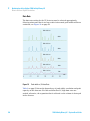
delay volume significantly, see Figure 17 on page 49.
b6J
AdlYZaVnkdajbZhZije 69KG
AdlYZaVnkdajbZhZije
HiVcYVgYhZije 69KG
HiVcYVgYhZije
B^c
Figure 17
Reduction of the delay volume
The lower the flow rate, the greater the negative impact that can be expected
from delay volume. In Figure 17 on page 49, a 2.1 mm inner diameter column
was used at a flow rate of 0.6 mL/min. The delay volume is reduced step by
step from the lowest trace to the top trace. The influence on total run time,
and the impact, especially on peak width and the heights of the first peaks, is
obvious.
The drawback of overlapped injection and automatic delay volume reduction
is that the autosampler is not in the flow path for the complete run time. For
very sticky compounds this could lead to higher carry-over and/or compound
discrimination.
1260 Infinity Binary LC - System User Guide
49
3
Optimization of the Agilent 1260 Infinity Binary LC
How to Achieve Shorter Cycle Times
Carry-over is the percentage of compound that remains in the parts of the
instrument that come into contact with the sample, and is not flushed onto the
column for analysis. It also means that this percentage is lost for quantitative
measurement; it is discriminated. The carry-over can be measured by injecting
pure solvent after the sample run is finished. Discrimination and carry-over
can become even more important if the analyte compounds are non-polar and
the start of the gradient contains a high percentage of water. In the worst case,
the non-polar compound precipitates at the surface of contact. Small plugs of,
for example, dimethylsulfoxide before and after the sample plug can help to
minimize this problem.
For overlapped injection or automated delay volume reduction, the time
before the injection valve is switched to the bypass mode should be increased
using the flush out factor to 20. This extends the time during which the
autosampler delay volume is flushed with mobile phase.
How to Achieve High Throughput
The injection can be optimized for speed remembering that drawing the
sample too fast can reduce the reproducibility. Marginal gains are to be made
here as the sample volumes used tend towards the smaller end of the range in
any case. A significant portion of the injection time is the time taken with the
needle movements to and from the vial and into the flush port. These
manipulations can be performed while the previous separation is running.
This is known as "overlapped injection" and it can be easily turned on from the
autosampler setup screen in the control software. The autosampler can be told
to switch the flow through the autosampler to bypass after the injection has
been made and then after, for example, 3 minutes into a 4 minutes run to start
the process of aspirating the next sample and preparing for injection. This can
typically save 0.5 to 1 minute per injection.
50
1260 Infinity Binary LC - System User Guide
3
Optimization of the Agilent 1260 Infinity Binary LC
How to Achieve Lowest Carry-over
How to Achieve Lowest Carry-over
Carryover is measured when residual peaks from a previous active-containing
injection appear in a subsequent blank solvent injection. There will be
carryover between active injections which may lead to erroneous results. The
level of carryover is reported as the area of the peak in the blank solution that
is expressed as a percentage of the area in the previous active injection. The
Agilent 1260 Infinity Autosampler is optimized for lowest carryover by careful
design of the flow path and use of materials in which sample adsorption is
minimized. A carryover figure of 0.002 % should be achievable even when a
triple quadrupole mass spectrometer is the detector. Operating settings of the
autosampler allow the user to set appropriate parameters to minimize
carryover in any application involving compounds liable to stick in the system.
The following functions of the autosampler can be used to minimize carryover:
• Internal needle wash
• External needle wash
• Needle seat backflush
• Injection valve cleaning
The flow path, including the inside of the needle, is continuously flushed in
normal operation, providing good elimination of carryover for most situations.
Automated delay volume reduction (ADVR) will reduce the delay volume but
will also reduce the flushing of the autosampler and should not be used with
analytes where carryover might be a problem.
To ensure lowest carry-over, consider the following recommendations:
• Always use the autosampler with the injection valve in mainpass position.
• Flush the exterior of the needle with an appropriate solvent using the flush
port. The flush time should be a minimum of 10 s.
• If possible, reduce the draw speed to 10 μL/min.
• Use Agilent capped 2 mL vials (Screw cap vial, 2 mL (5182-0556)).
• If the seat is contaminated, use an appropriate seat-flush procedure.
• Use flushing solvents that are capable of dissolving the sample compounds.
• Use acidic mobile phases for basic compounds.
1260 Infinity Binary LC - System User Guide
51
3
Optimization of the Agilent 1260 Infinity Binary LC
How to Achieve Lowest Carry-over
Flushing and cleaning of the autosampler to achieve near zero carry-over
During the injection routine, the sample loop, the inside of the needle, the seat
capillary, and the main channel of the injection valve are in the flow path, and
remain there throughout the duration of the run. This means that these parts
are flushed continuously with mobile phase during the complete analysis. It is
only during aspiration of the sample that the injection valve is switched out of
the flow path. In this position, the pump effluent is led directly to the column.
Prior to injection, the outside surfaces of the needle are washed with fresh
solvent. This is achieved using the flush port of the autosampler, and prevents
contamination of the needle seat. The flush port of the autosampler is refilled
with fresh solvent by a peristaltic pump that is installed in the autosampler
housing. The flush port has a volume of about 680 μL, and the pump delivers
6 mL/min. Setting the wash time to 10 s means that the flush port volume is
refilled more than once with fresh solvent, which is sufficient in most cases to
clean the outside of the needle.
52
1260 Infinity Binary LC - System User Guide
Optimization of the Agilent 1260 Infinity Binary LC
How to Achieve Higher Resolution
3
How to Achieve Higher Resolution
Increased resolution in a separation will improve the qualitative and
quantitative data analysis, allow more peaks to be separated or offer further
scope for speeding up the separation. This section explains how resolution can
be increased by examining the following points:
• Optimize selectivity
• Smaller particle-size packing
• Longer columns
• Shallower gradients, faster flow
• Minimal extra-column volume
• Optimize injection solvent and volume
• Fast enough data collection
Resolution between two peaks is described by the resolution equation:
where
• Rs=resolution,
• N=plate count (measure of column efficiency),
• α=selectivity (between two peaks),
• k2=retention factor of second peak (formerly called capacity factor).
The term with the most significant effect on resolution is the selectivity, α, and
practically varying this term involves changing the type of stationary phase
(C18, C8, phenyl, nitrile etc.), the mobile phase and temperature to maximize
the selectivity differences between the solutes to be separated. This is a
substantial piece of work which is best done with an automated method
development system which allows a wide range of conditions on different
columns and mobile phases to be assessed in an ordered scouting protocol.
This section considers how to get higher resolution with any chosen stationary
and mobile phases. If an automated method development system was used in
the decision on phases, it is likely that short columns were used for fast
analysis in each step of the scouting.
1260 Infinity Binary LC - System User Guide
53
3
Optimization of the Agilent 1260 Infinity Binary LC
How to Achieve Higher Resolution
The resolution equation shows that the next most significant term is the plate
count or efficiency, N, which can be optimized in a number of ways. N is
inversely proportional to the particle size and directly proportional to the
length of a column and so smaller particle size and a longer column will give a
higher plate number. The pressure rises with the inverse square of the particle
size and proportionally with the length of the column. Resolution increases
with the square root of N so doubling the length of the column will increase
resolution by a factor of 1.4 . What is achievable depends on the viscosity of
the mobile phase as this relates directly to the pressure. Methanol mixtures
will generate more back pressure than acetonitrile mixtures. Acetonitrile is
often preferred because peak shapes are better and narrower in addition to
the lower viscosity but methanol generally yields better selectivity (certainly
for small molecules less than about 500 Da). The viscosity can be reduced by
increasing the temperature but it should be remembered that this can change
the selectivity of the separation. Experiment will show if this leads to increase
or decrease in selectivity. As flow and pressure are increased, it should be
remembered that frictional heating inside the column will increase. That can
lead to slightly increased dispersion and possibly a small selectivity change
both of which could be seen as a reduction in resolution. The latter case might
be offset by reducing the temperature of the thermostat by a few degrees and
again experiment will reveal the answer.
The van Deemter curve shows that the optimum flow rate through an STM
column is higher than for larger particles and is fairly flat as the flow rate
increases. Typical, close to optimum, flow rates for STM columns are:
2 ml/min for 4.6 mm i.d.; and 0.4 ml/min for 2.1 mm i.d. columns.
54
1260 Infinity Binary LC - System User Guide
3
Optimization of the Agilent 1260 Infinity Binary LC
How to Achieve Higher Resolution
In isocratic separations, increasing the retention factor, k, results in better
resolution because the solute is retained longer. In gradient separations, the
retention is described by k* in the following equation:
where:
• k* = mean k value,
• tG = time length of gradient (or segment of gradient) (min),
• F = flow (ml/min),
• Vm = column delay volume,
• Δ%B = change in fraction of solvent B during the gradient,
• S = constant (ca. 4-5 for small molecules).
This shows that k and hence resolution can be increased by having a shallower
gradient (2 to 5 %/min change is a guideline), higher flow rate and a smaller
volume column. This equation also shows how to speed up an existing gradient
– if the flow is doubled but the gradient time is halved, k* remains constant
and the separation looks the same but happens in half the time.
Any reduction in extra-column volume will reduce dispersion and give better
resolution. This is already optimized in the 1260 Infinity Binary LC with
narrow bore (0.12 mm i.d.) capillaries (check that the shortest length is used
between column and detector) and the Max-light cartridge flow cell.
Finally, any gains in resolution must be preserved by having data collection
which is fast enough to accurately profile the narrow peaks.
In summary, the following steps should be considered to increase resolution:
• The first step in improving resolution is always to test different stationary
phases and to select the column with the best separation. This is the
parameter that is of most importance for resolution.
• The second step is to use long columns or even coupled columns to increase
the plate number.
• A third step is to shift peaks to higher retention factors. For k values of 5 to
10, the impact is significant. With higher k values, the effect is very low.
In practice, this means that longer columns with appropriate selectivity give
better resolution.
1260 Infinity Binary LC - System User Guide
55
3
Optimization of the Agilent 1260 Infinity Binary LC
How to Achieve Higher Resolution
Optimum Instrument Configuration for High Resolution
Column Compartment
The column compartment can be used in its standard version for 4.6 mm inner
diameter columns. At flow rates above 2 mL/min, and temperatures above
60 °C, the column effluent should be cooled down to the temperature of the
detector by using the 1.5 μL cooler/heater in the column compartment. This
ensures lowest noise level with UV detectors, even at 5 mL/min and 80 °C (see
Figure 18 on page 56 ).
Cdgb#
L^i]edhiXdajbcXdda^c\
Cd^hZEidE2%#-'-.b6J
CdedhiXdajbcXdda^c\ H$C[dgeZV`)2)-'
Cd^hZEidE2&#*.%*b6J
H$C[dgeZV`)2(.'
8dda^c\cZZYZY3'ba$b^c
b^c
Figure 18
Influence of post column cooling (PCC) on baseline noise
If 2.1 mm inner diameter columns are used at low flow rates, the small heating
device should be used for lowest extra-column volume.
56
1260 Infinity Binary LC - System User Guide
Optimization of the Agilent 1260 Infinity Binary LC
How to Achieve Higher Resolution
3
Extra-column Volume
To maintain the high resolution achieved on the column, the extra-column
volume, especially after the column, should be as low as possible.
• For 4.6 mm inner diameter columns the standard delay configuration
should be used for the pump, see Figure 15 on page 45.
• For 2.1 mm inner diameter columns, the low delay configuration should be
used for the pump, and the low dispersion kit should be installed in the
column compartment. For highest UV sensitivity, the short mixer is also
recommended. See Figure 13 on page 43 and Figure 14 on page 44.
• The injection volume is also of importance, especially if the sample is
dissolved in an organic solvent. In this case, the gradient should start with a
low percentage of organic phase to focus the compounds at the top of the
column. This avoids peaks dispersion due to the injection.
• The 10 mm Max-Light cartridge cell has a low dispersion volume (σ volume
1.0 μL) and no further volume optimization is required.
• In situations where the alternative 60 mm Max-Light high sensitivity cell is
used to get higher sensitivity the cell volume is optimized for the use with
3 mm and 4.6 mm inner diameter columns.
1260 Infinity Binary LC - System User Guide
57
3
Optimization of the Agilent 1260 Infinity Binary LC
How to Achieve Higher Resolution
Data Rate
The data rate setting for the UV detector must be selected appropriately.
Selecting a data rate that is too low results in increased peak width and lower
resolution, see Figure 19 on page 58.
EL2%#(%hZX
-%=o
EL2%#((hZX
)%=o
EL2%#)'hZX
'%=o
EL2%#+,hZX
&%=o
EL2&#')hZX
*=o
b^c#
Figure 19
Peak width vs, UV data Rate
Table 6 on page 59 shows the dependency of peak width, resolution and peak
capacity on the data rate. For fast and ultra-fast LC, high data rates are
needed; otherwise, the separation that is achieved on the column is destroyed
in the detector.
58
1260 Infinity Binary LC - System User Guide
Optimization of the Agilent 1260 Infinity Binary LC
How to Achieve Higher Resolution
Table 6
3
Relation between data rate and chromatographic performance
Data Rate
Peak Width
Resolution
Peak Capacity
80 Hz
0.300
2.25
60
40 Hz
0.329
2.05
55
20 Hz
0.416
1.71
45
10 Hz
0.666
1.17
29
5 Hz
1.236
0.67
16
80 Hz data rate compared with 20 Hz data rate results in improvements in:
• Peak Width:
– 30 %
• Resolution:
+ 30 %
• Peak capacity:
+ 40 %
• Apparent column efficiency:
+ 70 %
Chromatographic Conditions
As already stated previously, chromatographic conditions depend on the
compounds to be analyzed. But here also, some rules of thumb exist.
• Moderate flow rates should be used, but recent experiments have shown
that elevated flow rates can also be advantageous for improved separation.
For 4.6 mm inner diameter columns packed with sub-2-micron particles, a
flow rate of 2 mL/min is recommended as a starting value. For 2.1 mm
inner diameter sub-2-micron columns, 0.4 mL/min is a good starting point.
• Moderate gradients should be used, for example, 2 – 5 % gradient change
per minute.
• The column temperature is an additional parameter for optimization.
Temperature can influence a separation, and should not be overlooked.
1260 Infinity Binary LC - System User Guide
59
3
Optimization of the Agilent 1260 Infinity Binary LC
How to Achieve Higher Sensitivity
How to Achieve Higher Sensitivity
The sensitivity of a separation method is linked to the choice of stationary and
mobile phases as good separation with narrow peaks and a stable baseline
with minimal noise are desirable. The choice of instrument configuration will
have an effect and a major impact is the setup of the detector.
60
1260 Infinity Binary LC - System User Guide
3
Optimization of the Agilent 1260 Infinity Binary LC
How to Achieve Higher Sensitivity
Optimum Instrument Configuration for High Sensitivity
General Considerations
• To achieve lowest baseline noise, the standard delay volume configuration
is recommended for the 1260 Infinity Binary Pump.
• Here also, the injection volume and the sample dissolution solvent are
important. Care must be taken that the compounds are focused at the top of
the column, to avoid peak dispersion due to the injection, which would
cause a reduced peak height. In order to achieve this, the sample should be
dissolved in a solvent composition of lower elution strength than the mobile
phase.
• The column temperature should not be too low, to avoid long retention of
the peaks on the column. This also creates peak dispersion and a lower
peak height.
• The data rate of the UV detector should be selected according to the actual
peak width. Higher than necessary data rates should be avoided because of
higher noise levels.
• Available UV detectors are the Agilent 1260 Infinity Diode Array Detector
(G4212B) and the Agilent 1260 Infinity Variable Wavelength Detector
(G1314F), with data rates of 80 Hz and significantly lower noise and drift
levels.
• “Choosing a Flow Cell” on page 63 gives an overview of the flow cells
available with the G4212B DAD. For information on flow cells used with the
G1314F VWD, please refer to the User Manual of the Agilent 1260 Infinity
Variable Wavelength Detector.
Chromatographic Conditions
For an optimum signal-to-noise ratio, it is of advantage if the peaks elute
quickly.
• Elevated flow rates should be used to elute the peaks at low k’values.
• Faster gradients can also be applied to elute the peaks at low k’values.
1260 Infinity Binary LC - System User Guide
61
3
Optimization of the Agilent 1260 Infinity Binary LC
How to Achieve Higher Sensitivity
Columns
Sensitivity is specified as a signal-to-noise ratio (S/N) and hence the need to
maximize peak height and minimize baseline noise. Any reduction in peak
dispersion will help to maintain peak height and so extra-column volume
should be minimized by use of short, narrow internal diameter, connection
capillaries and correctly installed fittings. Using smaller inner diameter
columns should result in higher peak height and is therefore ideal for
applications with limited sample amounts. If the same sample amount can be
injected on a smaller i.d. column, then the dilution due to column diameter
will be less and the sensitivity will increase. For example, decreasing the
column i.d. from 4.6 mm to 2.1 mm results in a theoretical gain in peak height
of 4.7 times due to the decreased dilution in the column. For a mass
spectrometer detector, the lower flow rates of narrow columns can result in
higher ionization efficiencies and therefore higher sensitivity.
Detector Settings
The detector has a number of parameters that are used to optimize
performance. The following sections describe how the detector parameters
affect performance characteristics:
• Flow cell affects sensitivity,
• Wavelength and bandwidth affect sensitivity, selectivity and linearity,
• Slit Width affects sensitivity, spectral resolution and linearity,
• Peak Width affects sensitivity and resolution.
62
1260 Infinity Binary LC - System User Guide
3
Optimization of the Agilent 1260 Infinity Binary LC
How to Achieve Higher Sensitivity
Choosing a Flow Cell
Several flavors of the Max-Light Cartridge Flow Cell are available, see (Table 7
on page 63).
Table 7
Specifications for Max-Light Cartridge Flow Cells
Cartridge Cells
•
•
•
•
•
•
•
Max-Light Cartridge Cell ( 10 mm, V(σ) 1.0 µL) (G4212-60008)
Max-Light Cartridge Cell Bio-inert ( 10 mm, V(σ) 1.0 µL) (G5615-60018)
Max-Light Cartridge Cell ( 60 mm, V(σ) 4.0 µL) (G4212-60007)
Max-Light Cartridge Cell Bio-inert ( 60 mm, V(σ) 4.0 µL) (G5615-60017)
HDR Max-Light Cartridge Cell ( 3.7 mm, V(σ) 0.4 µL) (G4212-60032)
ULD Max-Light Cartridge Cell ( 10 mm, V(σ) 0.6 µL) (G4212-60038)
Max-Light Cartridge Test Cell (G4212-60011)
Maximum
pressure
70 bar (1015 psi) Maximum Operating Pressure (MOP)1
150 bar (2175 psi) Maximum Incidential Pressure (MIP)2
pH range
1.0-12.5 (solvent dependent)
1
Maximum Operating Pressure (MOP): The maximum pressure at which the system can operate
continuously under normal conditions.
2
Maximum Incidential Pressure (MIP): The maximum pressure which the system can experience
during a short time.
Normal Applications
The Max-Light Cartridge Cell ( 10 mm, V(σ) 1.0 μL) (G4212-60008) covers a
wide range of applications:
• all column diameter down to at least 2.1 mm ID or even less
• applications with peak dispersion (Peakwidth x flow) down to ~2 μL
[example: pw = 0.04 min at flow = 0.1 mL/min gives peak dispersion of
0.04 min x 0.1 mL/min = 0.004 mL = 4 μL]
High Sensitiviy
If higher sensitivity is necessary, the Max-Light Cartridge Cell ( 60 mm,
V(σ) 4.0 μL) (G4212-60007) can be used. This cell enhances the detector by
lowering the limit of detection (LOD) by a factor of about 3 (depending on the
application).
1260 Infinity Binary LC - System User Guide
63
3
Optimization of the Agilent 1260 Infinity Binary LC
How to Achieve Higher Sensitivity
Ultra-Low Dispersion
The Max-Light Cartridge ULD cell can be used with the G4212A DAD and
G4212B DAD. The cell is a requirement for the Ultra-Low Dispersion Kit
solution which currently exists as 1290 Infinity Ultra-Low Dispersion Kit
(5067-5189). The cell should be part of the ultra-low dispersion solution.
High Dynamic Range
The Max-Light Cartridge HDR cell can be used with the G4212A DAD and
G4212B DAD. The cell is required as a part of the High Dynamic Range (HDR)
solution which will be introduced March/April 2013.
NOTE
64
To protect the flow cell against overpressure (e.g. in systems with LC/MS) install Inline
Pressure Relief Valve Kit (G4212-68001), see Agilent 1200 Infinity Series Diode Array
Detectors manual.
1260 Infinity Binary LC - System User Guide
3
Optimization of the Agilent 1260 Infinity Binary LC
How to Prevent Column Blockages
How to Prevent Column Blockages
Columns packed with sub-2-micron particles also need frits with small pore
size to prevent packing material being swept out. This immediately brings
increased risk of blocking these frits with particulates from the sample, mobile
phase or/and from the instrument itself. To protect the column, additional
small filters ( Figure 20 on page 66) can be used in front of the column. It is
also recommended that the sample is thoroughly filtered or/and centrifuged,
and that any kind of particulate matter in the mobile phases is avoided.
To ensure best results follow these simple usage guidance:
1 Install and run the column only in the flow direction marked on the
column.
2 Use only solvents that are high quality, chromatography grade.
3 Filter all aqueous buffers and all samples through an appropriate 0.2 μm
filter before use.
4 Replace bottles of mobile phase buffer every 24 – 48 h — do not add mobile
phase to the bottle; always use a new bottle.
5 Do not use a high buffer salt mobile phase (> 50 mM) in combination with
high acetonitrile concentrations due to possible precipitation.
6 An in-line filter is recommended to catch particulates and extend column
life. Use the suitable 1260 Infinity In-line filter for your column: 1260
Infinity LC in-line filter, 2.1 mm, 0.2 μm pore size filter, max 600 bar,
connecting capillary 70 x 0.12 mm SS (5067-1551) for 2.1 i.d. columns, 1260
Infinity LC in-line filter, 4.6 mm, 0.2 μm pore size filter, max 600 bar,
connecting capillary 90 x 0.17 mm SS (5067-1553) for 4.6 mm or 3.0 mm i.d.
columns. Change the filter when the pressure increases by 10 %.
7 Purge the pumps (the connections up to the column) of any buffer
containing mobile phases and flush through 5 mL of solvent before
attaching the column to the instrument.
8 Flush the column with compatible mobile phase starting slowly at
0.1 mL/min for a 2.1 mm inner diameter column, 0.2 mL/min for a 3.0 mm
inner diameter column, and 0.4 mL/min for 4.6 mm inner diameter.
Increase the flow rate to the desired flow over 5 minutes.
9 Once the pressure has stabilized, attach the column to the detector.
10 Equilibrate the column and detector with 10 column volumes of the mobile
phase prior to use. (1 – 5 mL depending on column size.)
11 Avoid over-pressure. Check the pressure range of your gradient — which
may be 100 – 130 bar or more — before starting any sequence.
1260 Infinity Binary LC - System User Guide
65
3
Optimization of the Agilent 1260 Infinity Binary LC
How to Prevent Column Blockages
;dg'#&bb;g^ihjhZ
^chZgihl^i]
hbVaaXdcZ
;dg)#+bb;g^ihjhZ^chZgih
l^i]W^\XdcZ
Figure 20
66
Protection for 4.6 and 2.1 mm id columns packed with 1.8 µm particles, inlet
frit with 0.2 µm pore size
1260 Infinity Binary LC - System User Guide
1260 Infinity Binary LC - System User Guide
4
System Setup and Installation
Installing Software
68
Installing the Modules 70
Installing the System Modules 70
Integration Into the Network 70
Capillary and Tubing Connections in Flow Path
Priming the System 76
71
This chapter includes information on software installation, installation of the
modules, and preparing the system for operation.
Agilent Technologies
67
4
System Setup and Installation
Installing Software
Installing Software
Installing the Software Controller and Data System
For details of installation procedures for the software, refer to the detector
manual and the software manuals.
68
1260 Infinity Binary LC - System User Guide
4
System Setup and Installation
Installing Software
Installing the Agilent Lab Advisor Software
For details of installation procedures for the Agilent Lab Advisor software,
refer to the software documentation on the Lab Advisor DVD.
Agilent Lab Advisor replaces and extends the diagnostic functions that were
formerly available only in the ChemStation software.
Agilent Lab Advisor is a Windows-based application that continuously
monitors instruments in the lab in real time and increases productivity
through automatic notification of maintenance and service needs with the use
of advanced counters. This allows a problem to be fixed before it impacts
results. The software includes an extensive suite of user information and
documentation, a set of calculators and tools to help set up, calibrate, and
maintain your instrument, and tests and diagnostic routines to verify proper
performance. Agilent Lab Advisor also provides feedback and solutions for
any instrument errors that may arise. The software will work with or without
Agilent data systems.
The software monitors:
• LC module status
• Early Maintenance Feedback (to determine the need for upgrade or
replacement)
In addition, the software:
• Automates useful tests,
• Attempts to identify supported LAN-based instruments that are powered
on and connected to your PC or lab’s network,
• Automatically suggests replacements parts and troubleshooting tasks for
some common instrument problems.
1260 Infinity Binary LC - System User Guide
69
4
System Setup and Installation
Installing the Modules
Installing the Modules
Installing the System Modules
For details of installation procedures for the modules, refer to the individual
module manuals. These manuals also contain information on specifications,
maintenance and parts.
Integration Into the Network
For network integration of your system refer to user manuals of your modules
(chapter LAN Configuration).
70
1260 Infinity Binary LC - System User Guide
System Setup and Installation
Installing the Modules
4
Capillary and Tubing Connections in Flow Path
Depending on the system configuration, capillaries of different lengths and
diameters are used. These are described below.
See module manuals for module-internal capillary and tubing connections.
1260 Infinity Binary LC - System User Guide
71
4
System Setup and Installation
Installing the Modules
Connections for Standard Delay Volume Configuration
Figure 21 on page 72 shows capillary and tubing connections in the flow path
for the standard delay volume configuration of the 1260 Infinity Binary LC.
HdakZciXVW^cZi
9Z\VhhZg
Ejbe
&
6jidhVbeaZg
I]ZgbdhiVi
'
I]ZgbdhiViiZY
XdajbcXdbeVgibZci
(
4
9ZiZXidg969
*
Figure 21
72
Capillary and tubing connections in flow path (standard delay volume
configuration)
1260 Infinity Binary LC - System User Guide
System Setup and Installation
Installing the Modules
Item
p/n
Description
1
G1312-87303
Capillary ST 0.17 mm x 400 mm S/S
(Pump to autosampler)
1
G1312-87304
Capillary ST 0.17 mm x 700 mm S/S
(Pump to cooled Autosampler)
2
G1367-87304
Capillary ST 0.17 mm x 250 mm S/S
(Autosampler to TCC)
2
01090-87306
Capillary ST 0.17 mm x 380 nm S/S
(Cooled Autosampler to TCC)
3
G1316-87300
Capillary ST 0.17 x 90 mm S/S
(TCC to Column)
4
G1315-87311
Capillary ST 0.17 mm x 380 mm S/S
(Column to DAD)
5
5062-2462
Tube PTFE 0.8 mm x 2 m, re-order 5 m
(DAD to waste)
5
5062-8535
Waste accessory kit
(VWD to waste)
1260 Infinity Binary LC - System User Guide
4
73
4
System Setup and Installation
Installing the Modules
Connections for Medium and Low Delay Volume Configuration
Figure 22 on page 74 shows capillary and tubing connections in the flow path
for medium and low delay volume configurations of the 1260 Infinity Binary LC.
HdakZciXVW^cZi
9Z\VhhZg
Ejbe
&
6jidhVbeaZg
'
I]ZgbdhiVi
(
I]ZgbdhiViiZYXdajbc
XdbeVgibZci
)
*
9ZiZXidg969
+
Figure 22
74
Capillary and tubing connections in flow path (medium and low delay volume
configurations)
1260 Infinity Binary LC - System User Guide
System Setup and Installation
Installing the Modules
Item
p/n
Description
1
G1312-87303
Capillary ST 0.17 mm x 400 mm S/S
(Pump to autosampler)
1
G1312-87304
Capillary ST 0.17 mm x 700 mm S/S
(Pump to cooled Autosampler)
2
G1313-87304
Capillary ST 0.12 mm x 180 mm S/S
(Autosampler to TCC)
2
01090-87610
Capillary ST 0.12 mmx 280 mm S/S
(cooled Autosampler to TCC or to item 3 if installed)
3
G1316-80002
Heater long-up (0.12 mm i.d., 1.6 µL internal volume)
3
G1316-80003
Heater long-down (0.12 mm i.d., 1.6 µL internal volume)
4
01090-87611
Capillary ST 0.12 mmx 105 mm S/S
(TCC to Column, not needed if item 3 is installed)
5
G1315-87312
Capillary ST 0.12 mm x 150 mm S/S
(Column to DAD)
6
5062-2462
Tube PTFE 0.8 mm x 2 m, re-order 5 m
(DAD to waste)
1260 Infinity Binary LC - System User Guide
4
75
4
System Setup and Installation
Installing the Modules
Priming the System
Initial Priming
When
Before a degasser or solvent tubing can be used, it is necessary to prime the system. Isopropanol is
recommended as priming solvent due to its miscibility with nearly all HPLC solvents and its
excellent wetting properties.
Parts required
Preparations
#
Description
1
Isopropanol
Connect all modules hydraulically as described in the respective module manuals.
Fill each solvent bottle with 100 mL isopropanol
Switch the system on
WA R N I N G
When opening capillary or tube fittings, solvents may leak out.
The handling of toxic and hazardous solvents and reagents can carry health risks.
➔ Observe appropriate safety procedures (for example, wear goggles, safety gloves
and protective clothing) as described in the material handling and safety data sheet
supplied by the solvent vendor, especially when toxic or hazardous solvents are
used.
76
NOTE
The purge tool of the Lab Advisor can be used to purge the pump automatically.
NOTE
If the pump is not able to draw in the solvent from the bottles, use a syringe to move the
solvent manually through tubing and degasser.
NOTE
When priming the vacuum degasser with a syringe, the solvent is drawn through the
degasser tubes very quickly. The solvent at the degasser outlet will therefore not be fully
degassed. Pump for approximately 10 minutes at your desired flow rate before starting an
analysis. This will allow the vacuum degasser to properly degas the solvent in the degasser
tubes.
1260 Infinity Binary LC - System User Guide
System Setup and Installation
Installing the Modules
4
1 Open the purge valve of the pump
2 Set the flow rate to 5 mL/min.
3 Select channel A1
4 Turn the flow on
5 Observe if the solvent in the tubing of channel A1 is advancing towards the
pump. If it isn’t, disconnect the solvent tubing from the solvent selection
valve, attach a syringe with a syringe adapter and pull the liquid through
the degasser. Reattach the tubing to the solvent selection valve.
6 Pump 30 mL isopropanol to remove residual air bubbles.
7 Switch to the next solvent channel and repeat steps 5 and 6 until all
channels have been purged.
8 Turn the flow off and close the purge valve.
1260 Infinity Binary LC - System User Guide
77
4
System Setup and Installation
Installing the Modules
Regular Priming
When
When the pumping system has been turned off for a certain time (for example, overnight) air will
rediffuse into the solvent channel between the vacuum degasser and the pump. If solvents
containing volatile components are left in the degasser without flow for a prolonged period, there
will be a slight loss of the volatile components.
Preparations
Switch the system on
NOTE
The purge tool of the Lab Advisor can be used for automatically purging the pump.
1 Open the purge valve of your pump by turning it counterclockwise and set
the flow rate to 5 mL/min.
2 Flush the vacuum degasser and all tubes with at least 10 mL of solvent.
3 Repeat step 1 and 2 for the other channel(s) of the pump.
4 Set the required composition and flow rate for your application and close
the purge valve.
5 Pump for approximately 10 minutes before starting your application.
78
1260 Infinity Binary LC - System User Guide
4
System Setup and Installation
Installing the Modules
Changing Solvents
When
Parts required
When the solvent of a channel is to be replaced by another solvent that is not compatible (solvents
are immiscible or one solvent contains a buffer), it is necessary to follow the procedure below to
prevent clogging of the pump by salt precipitation or residual liquid droplets in parts of the system.
#
p/n
1
1
Preparations
Description
Purging solvent(s), see Table 8 on page 80
5022-2184
Union ZDV
Remove the column and replace it by a ZDV fitting
Prepare bottles with appropriate intermediate solvents (see Table 8 on page 80)
1 If the channel is not filled with buffer, proceed to step 4.
2 Place the solvent intake filter into a bottle of water.
3 Flush the channel at a flow rate suitable for the installed tubing (typically
3 – 5 mL/min) for 10 min.
4 Modify the flow path of your system as required for your application.
CAUTION
Buffer salt of aqueous buffers may precipitate in residual isopropanol.
Capillaries and filter may be clogged by precipitating salt.
➔ Flush solvent lines containing high concentration of salts first with water before
introducing organic solvent.
➔ Do not perform steps 5 to 7 for channels running with aqueous buffer as solvent.
5 Replace the solvent bottle by a bottle of isopropanol.
6 Flush the channel at a flow rate suitable for the installed tubing (typically
3 – 5 mL/min) for 5 min.
7 Swap the bottle of isopropanol with a bottle of solvent for your application.
8 Repeat steps 1 to 7 for the other channel(s) of the pump.
9 Install the desired column, set the required composition and flow rate for
your application and equilibrate the system for approx. 10 minutes prior to
starting a run.
1260 Infinity Binary LC - System User Guide
79
4
System Setup and Installation
Installing the Modules
Table 8
80
Choice of Priming Solvents for Different Purposes
Activity
Solvent
Comments
After an installation
When switching between
reverse phase and normal
phase (both times)
Isopropanol
Isopropanol
Best solvent to flush air out of
the system
Miscible with almost all
solvents
After an installation
Ethanol or methanol
Alternative to isopropanol
(second choice) if no
isopropanol is available
To clean the system when
using buffers
After changing aqueous
solvents
HPLC grade water
Best solvent to re-dissolve
buffer crystals
Best solvent to re-dissolve
buffer crystals
After the installation of normal
phase seals (PE seals
(pack of 2) (0905-1420))
Hexane + 5 % isopropanol
HPLC grade water
Good wetting properties
1260 Infinity Binary LC - System User Guide
1260 Infinity Binary LC - System User Guide
5
Quick Start Guide
About the Quick Start Guide
82
Preparing the System 83
Turning the System ON 83
Loading the Default Method 84
Configuring the Online Plot 85
Purging the Pump 87
Data Acquisition in Method and Run Control View 88
Method Parameters for System Checkout with Isocratic Checkout
Sample 88
Setting Up the Method 92
Running the Method for a Single Injection 94
Data Analysis 96
Data Analysis View 97
Integrating a Signal 98
Specify the Report 99
This chapter provides information on data acquisition and data analysis with
the 1260 Infinity Binary LC.
Agilent Technologies
81
5
Quick Start Guide
About the Quick Start Guide
About the Quick Start Guide
This chapter provides information on running the Agilent 1260 Infinity Binary
LC. It can be used as a guide to quickly running a first analysis after
installation, serving both as a tutorial example and a check on the overall
functioning of the system. It also includes more detailed information about
method parameters.
This example demonstrates setting up and running an analysis using the
columns and checkout sample that are provided with the Agilent 1260 Infinity
Binary LC. The example refers to menus and commands in OpenLAB CDS
ChemStation Edition, but identical functions are also available on the
alternative control options such as OpenLAB CDS EZChrom Edition and
MassHunter software.
In the following, the terms ChemStation and EZChrom always refer to Agilent
OpenLAB CDS ChemStation Edition and Agilent OpenLAB CDS EZChrom
Edition respectively.
NOTE
82
The starting point assumes that the system has been installed, turned on and initially
primed (see “Initial Priming” on page 76). The UV lamp should be turned on at least 30
minutes before starting any quantitative work.
1260 Infinity Binary LC - System User Guide
5
Quick Start Guide
Preparing the System
Preparing the System
Turning the System ON
If the system is not already fully on with the software showing Ready status,
follow these steps:
1 Turn on the computer system and wait for the Windows desktop to appear.
2 Turn on the electrical power to the LC modules using the button at the
lower left of each module.
A green power on light will be visible in the center of the button.
3 Start the control software on the computer by clicking the icon (if
configured). Alternatively, you can select Start > All Programs > Agilent
Technologies > OpenLAB > OpenLAB Control Panel. Select the relevant
instrument in the navigation pane under Instruments, and click Launch online.
The ChemStation software opens in the Method and Run Control view. The
modules are initially in Standby mode and Not Ready status, except for the
autosampler which immediately initializes and becomes Ready.
4 To switch on each module individually, right-click the relevant icon and
select Switch [module name] on from the context menu.
Alternatively, you can turn on all modules simultaneously in the system by
clicking the System On/Off button in the bottom right of the system diagram.
The system status changes from Not Ready (yellow indication) to Ready
(green indication) after a short delay as the setpoints are attained.
1260 Infinity Binary LC - System User Guide
83
5
Quick Start Guide
Preparing the System
Loading the Default Method
The ChemStation has a default method named DEF_LC.M which is loaded at
first execution or whenever a new blank method template is required. It
contains default settings for all modules.
With this procedure, you load the method DEF_LC.M. You can use it to set all
parameters to default settings, or to get a blank method template before
setting up a new method.
1 Go to Method and Run Control view of the ChemStation.
2 On the menu bar, select Method > New Method..., and select DEF_LC.M from
the context menu.
Alternatively, you can use the Load Method icon
under the menu bar, or
double-click the method name DEF_LC.M in the Methods tab of the
Navigation Pane.
The default method (DEF_LC.M) has a set of default parameters which can then
be modified to create a new method. For instance, the flow rate is set to zero,
and the Method Information and Method History are blank.
NOTE
84
Note that this method can never be overwritten with new parameters. Hence clicking on
Save will re-direct you into the Save As... function, so that you must enter a different
method name.
1260 Infinity Binary LC - System User Guide
5
Quick Start Guide
Preparing the System
Configuring the Online Plot
1 If the Online Plot window is not visible: Click View > Online Signals > Signal
Window 1 to display the window.
2 To configure the desired signal(s) in the Online Plot window, click Change….
The Edit Signal Plot setup page opens.
1260 Infinity Binary LC - System User Guide
85
5
Quick Start Guide
Preparing the System
3 In the Available Signals box, highlight the required signal(s), and click Add to
move them to the Selected Signals box.
4 To configure the individual settings for each signal, highlight the signal in
the Selected Signal box and set the required values in the lower half of the
page.
NOTE
In addition to the detector signals, parameter traces such as temperature and pressure can
also be plotted. With Apply to Method, the settings in this page can be stored into the
method.
The Online Plot window behaves like electronic chart paper, continuously
recording the output from the detector(s) and other output parameters. The
signals are drawn at the right of the window and move away to the left. Up to
90 min of past data is accessible. This is useful for checking the baseline and
looking at previous injections. The X and Y-axis scales can be adjusted directly
with the up/down buttons on each axis.
The Adjust button in the Online Plot window moves the current point on the
selected signal to the zero line. The selected signal is indicated by the color of
the Y-axis labels. A particular signal may be selected by clicking on the signal
or by clicking on the relevant signal description at the top of the plot.
The Balance button zeroes all detectors when pressed.
NOTE
86
Changes made in the Online Plot page do not in any way affect the data stored into the
individual data files.
1260 Infinity Binary LC - System User Guide
Quick Start Guide
Preparing the System
5
Purging the Pump
Purge the pump, if ...
• The pump has been primed for the first time.
• The pump is to be purged with fresh solvent before using the system, or
when the solvent is to be exchanged for another.
• The pump has been idle for a few hours or more (air may have diffused into
the solvent lines and purging is recommended).
• The solvent reservoirs are refilled, and the pump requires purging to fill the
system with fresh solvent. If different solvents are to be used, ensure that
the new solvent is miscible with the previous solvent and if necessary use
an intermediate step with a co-miscible solvent (isopropanol is often a good
choice, check with a solvent miscibility table).
For details on the purging procedure, refer to “Regular Priming” on page 78.
1260 Infinity Binary LC - System User Guide
87
5
Quick Start Guide
Data Acquisition in Method and Run Control View
Data Acquisition in Method and Run Control View
Method Parameters for System Checkout with Isocratic Checkout
Sample
For checkout of the 1260 Infinity Binary LC, a test run with an isocratic test
mixture (Agilent isocratic checkout sample (01080-68704)) will be performed
on the column ordered and delivered with your system.
Agilent isocratic checkout sample (01080-68704) contains the following
components dissolved in methanol:
• dimethyl phthalate
• diethyl phthalate
• biphenyl
• o-terphenyl
The method parameters for separation of this test mixture are summarized in
Table 9 on page 89 for the standard delay volume configuration and in
Table 10 on page 90 for the low delay volume configuration.
88
1260 Infinity Binary LC - System User Guide
5
Quick Start Guide
Data Acquisition in Method and Run Control View
Table 9
Method parameters for first separation run - standard delay volume configuration
Module
Parameter
Setting
Pump
Solvent A
Water
Solvent B
Acetonitrile
Flow rate
4.0 mL/min
Solvent
Composition
40 % A, 60 % B
Stop Time
1 min (1 min post time)
Autosampler
Injection
1 µL
Column
Compartment
Column
•
•
•
Detector
Column Eclipse Plus C18, 4.6 x 100 mm, 3.5 µm
(959961-902)
Column Poroshell 120 EC-C18, 3.0 x 50 mm, 2.7 µm
(699975-302)
Column Poroshell 120 EC-C18, 4.6 x 50 mm, 2.7 µm
(699975-902)
Temperature
40 °C
Signal A
Wavelength: 250 nm, Bandwidth: 4 nm
Reference Wavelength: 360 nm, Reference
Bandwidth: 100 nm
1260 Infinity Binary LC - System User Guide
89
5
Quick Start Guide
Data Acquisition in Method and Run Control View
Table 10
Method parameters for first separation run - low delay volume configuration
Module
Parameter
Setting
Pump
Solvent A
Water
Solvent B
Acetonitrile
Flow rate
0.75 mL/min
Solvent
Composition
40 % A, 60 % B
Stop Time
1.2 min (1 min post time)
Autosampler
Injection
1 µL
Column
Compartment
Column
Column: SB-C18, 4.6x 50 mm, 1.8 µm, 600 bar
(827975-902)
Temperature
40 °C
Signal
Wavelength: 250 nm, Bandwidth: 4 nm
Reference Wavelength: 360 nm, Reference
Bandwidth: 100 nm
Detector
Checkout specifications:
• four peaks are visible in the chromatogram
• Intensity Test – pass
• Wavelength Calibration ±1 nm
90
1260 Infinity Binary LC - System User Guide
5
Quick Start Guide
Data Acquisition in Method and Run Control View
Checkout Preparation
1 Fill solvent bottle A with HPLC grade Water. Fill solvent bottle B with HPLC
grade Acetonitrile.
2 If installed, purge each channel of the on-line degasser using the supplied
syringe.
3 Open the purge valve of the pump, and purge each channel at 5 mL/min.
This should be sufficient to remove air in the system.
4 Install the supplied column into the column compartment.
5 Flush the flow-cell with HPLC-grade water for 5 min.
6 Run a Wavelength Calibration and Intensity Test where applicable.
7 Allow the system to equilibrate at the checkout conditions listed in Table 9
on page 89 and Table 10 on page 90 for 10 min.
8 Prepare a vial of the isocratic checkout sample.
1260 Infinity Binary LC - System User Guide
91
5
Quick Start Guide
Data Acquisition in Method and Run Control View
Setting Up the Method
This section shows how to quickly set the method conditions for an analysis.
Prerequisites
The default method DEF_LC.M has been loaded ready to prepare the new method. Now the
key parameters can be edited to create the new method.
1 To quickly access the Method page for each module, right-click in the system
diagram for the module and select Method... from the context menu.
Each of the modules will be set up in this way.
2 Right-click the pump area, and select Method... in the context menu.
a In the Method page for the 1260 Infinity Binary Pump, enter the following
parameters:
• Flow rate: 4.0 ml/min
• Solvent A: Select Water from the compressibility drop-down list.
• Solvent B: Select the check box to make Solvent B active.
• Set the value for %B to 60 %
• Stop Time: 1 min
• Post Time: 1 min
b Other parameters can remain at their default settings. Click OK to exit
the window.
The changes are sent to the pump module.
3 Right-click the autosampler area, and select Method... in the context menu.
a In the Method page for the 1260 Infinity Autosampler, enter the following
parameters:
• Injection volume: 1.0 μl
• Injection with Needle Wash
• Mode Flush Port, Time: 6 s
b Other parameters can remain at their default settings. Click OK to exit
the window.
The changes are sent to the autosampler module.
92
1260 Infinity Binary LC - System User Guide
Quick Start Guide
Data Acquisition in Method and Run Control View
5
4 Right-click the Thermostatted Column Compartment (TCC) area, and select
Method... in the context menu.
a In the Method page for the 1290 Infinity TCC, enter the following
parameters:
• Left Temperature 40 °C
• Right Temperature Combined
b Other parameters can remain at their default settings. Click OK to exit
the window.
The changes are sent to the TCC module.
5 Right-click the Diode-Array Detector area, and select Method... in the
context menu.
a In the Method page for the 1260 Infinity DAD, enter the following
parameters:
• Use Signal: Turn all signals except Signal A off by clearing the check
boxes.
• Signal A: 254 nm, bw 4 nm, ref 550 nm, bw 100 nm
• Peak width: 0.02
b In the Advanced section, set Spectrum Store to All.
c Other parameters can remain at their default settings. Click OK to exit
the window.
The changes are sent to the DAD module.
6 All the required module parameters have now been entered. Select Method >
Save Method As... and enter
ISO-1.M to save the method with a new name.
The ChemStation does not allow the method to be saved as DEF_LC.M so that
the default method template is not altered.
7 Allow the system to equilibrate for at least 10 min, and check that the
baseline in the Online Plot is stable before starting the analysis.
1260 Infinity Binary LC - System User Guide
93
5
Quick Start Guide
Data Acquisition in Method and Run Control View
Running the Method for a Single Injection
This section shows how to run a single injection of the isocratic checkout
sample using the conditions entered in the previous section.
Analyses on the ChemStation can be run in two modes:
• Run Method — single injections, for example, in interactive method
development, using the parameter settings current at the time;
• Run Sequence — automated series of injections from multiple vials, possibly
with multiple methods. For further details refer to the ChemStation
manuals.
1 Click the Select Run Method Task icon
.
2 If required method conditions are not currently loaded, select Method > Load
Method or the icon
NOTE
under the menu bar to load them.
If changes have been made to a loaded method and not yet saved, this is indicated by a
yellow asterisk on the method status icon. The injection can be made without first saving
those parameters changes. The ChemStation always stores a copy of the acquisition
parameters in the data file as ACQ.TXT to ensure the preservation of the original method
parameters.
3 Place the sample vial in position 1 — this is the front position of the 10 x
2 ml vial positions on the right hand side of the sample tray.
4 Select Run Control > Sample Info, and enter the required sample parameters.
For example:
• Subdirectory (optional)
• Name Pattern
• Vial/Location
• Sample name
• Comment
5 If the system is already equilibrated and the baseline is stable, click Run
Method in the Sample Info page to start the injection. Alternatively, click OK,
and when ready, select Run Control > Run Method. The item will be added to
the Run Queue and then automatically started from there.
94
1260 Infinity Binary LC - System User Guide
Quick Start Guide
Data Acquisition in Method and Run Control View
5
6 The injection is made, and the chromatogram appears in the Online Plot. The
data acquisition will stop when the Stop Time is reached.
The chromatogram should look similar to the one below:
1260 Infinity Binary LC - System User Guide
95
5
Quick Start Guide
Data Analysis
Data Analysis
A method in the ChemStation contains all the parameters for data acquisition
(controlling the system) and data analysis (processing the data to give
quantitative and qualitative results). This section looks briefly at integration
and reports in data analysis so that the separations generated earlier in this
chapter can be integrated and printed. For more detailed information on data
analysis including the use of calibration for quantification refer to the
ChemStation manual.
BZi]dYhdjgXZ
CVk^\Vi^dciVWaZ
>ciZ\gVi^dciVh`
HeZXigjbiVh`
CVk^\Vi^dceVcZa
96
1260 Infinity Binary LC - System User Guide
5
Quick Start Guide
Data Analysis
Data Analysis View
To open a chromatogram in the Data Analysis view:
1 Launch an offline ChemStation.
2 Click Data Analysis in the bottom left of the screen.
3 In the Navigation Panel, find the data directory containing the data files.
All the single injection data are represented as a subset called Single Runs.
Double click Single Runs to load these data files into the Navigation Table.
4 Select a file in the Navigation Table, and double click it to load the
chromatogram into the viewer.
1260 Infinity Binary LC - System User Guide
97
5
Quick Start Guide
Data Analysis
Integrating a Signal
1 Select the Integration Task Tool (see figure below). The Integrate icon and
the Set Integration Events Table icon are highlighted in the figure shown below.
2 Click the Set Integration Events Table icon
to open the table as shown.
3 Set Baseline Correction to Advanced for gradient runs.
4 Set Slope Sensitivity to 5 .
Higher numbers will integrate steeper peaks and ignore less steep peaks.
5 Set the Peak Width value to the narrowest peak of interest, approximately
0.02 in this case.
6 Area Reject and Height Reject can be set to reject the smallest peaks.
7 Click the Integrate icon
to update the results using these new settings.
8 Exit from the Integration Events table using the green tick icon
98
.
1260 Infinity Binary LC - System User Guide
5
Quick Start Guide
Data Analysis
Specify the Report
1 On the menu bar click Report > Specify Report to display the window shown
in the figure below.
1260 Infinity Binary LC - System User Guide
99
5
Quick Start Guide
Data Analysis
2 With the example settings shown in the figures above you can produce an
Area Percent report on the screen.
3 In the Destination section, select Printer for a paper copy, and select File and
PDF to obtain a useful PDF report file stored into the datafile (the data file
with .D suffix is actually a directory. The report file can be viewed directly
in ChemStation or it can be found in the directory using the normal
Windows File Explorer).
4 Save the method once again to ensure the report settings are stored for
future use by the method.
When the method is used again, these integration events and report settings
will be used to produce the report.
This completes a brief look at using the Data Analysis part of the ChemStation
software. Consult the ChemStation manuals and the online help system for
further details about the powerful features of the ChemStation.
100
1260 Infinity Binary LC - System User Guide
1260 Infinity Binary LC - System User Guide
6
Appendix
Safety Information
102
Solvent Information 105
Material Information 105
Agilent Technologies on Internet
110
Setting Up a Method using Edit Entire Method
Method Information 113
Instrument/Acquisition 114
Data Analysis 129
Run Time Checklist 136
111
This chapter provides additional information on safety, legal and web and about
setting up a method.
Agilent Technologies
101
6
Appendix
Safety Information
Safety Information
General Safety Information
The following general safety precautions must be observed during all phases of
operation, service, and repair of this instrument. Failure to comply with these
precautions or with specific warnings elsewhere in this manual violates safety
standards of design, manufacture, and intended use of the instrument. Agilent
Technologies assumes no liability for the customer’s failure to comply with
these requirements.
WA R N I N G
Ensure the proper usage of the equipment.
The protection provided by the equipment may be impaired.
➔ The operator of this instrument is advised to use the equipment in a manner as
specified in this manual.
Safety Standards
This is a Safety Class I instrument (provided with terminal for protective
earthing) and has been manufactured and tested according to international
safety standards.
102
1260 Infinity Binary LC - System User Guide
6
Appendix
Safety Information
Operation
Before applying power, comply with the installation section. Additionally the
following must be observed.
Do not remove instrument covers when operating. Before the instrument is
switched on, all protective earth terminals, extension cords,
auto-transformers, and devices connected to it must be connected to a
protective earth via a ground socket. Any interruption of the protective earth
grounding will cause a potential shock hazard that could result in serious
personal injury. Whenever it is likely that the protection has been impaired,
the instrument must be made inoperative and be secured against any intended
operation.
Make sure that only fuses with the required rated current and of the specified
type (normal blow, time delay, and so on) are used for replacement. The use of
repaired fuses and the short-circuiting of fuse holders must be avoided.
Some adjustments described in the manual, are made with power supplied to
the instrument, and protective covers removed. Energy available at many
points may, if contacted, result in personal injury.
Any adjustment, maintenance, and repair of the opened instrument under
voltage should be avoided whenever possible. When inevitable, this has to be
carried out by a skilled person who is aware of the hazard involved. Do not
attempt internal service or adjustment unless another person, capable of
rendering first aid and resuscitation, is present. Do not replace components
with power cable connected.
Do not operate the instrument in the presence of flammable gases or fumes.
Operation of any electrical instrument in such an environment constitutes a
definite safety hazard.
Do not install substitute parts or make any unauthorized modification to the
instrument.
Capacitors inside the instrument may still be charged, even though the
instrument has been disconnected from its source of supply. Dangerous
voltages, capable of causing serious personal injury, are present in this
instrument. Use extreme caution when handling, testing and adjusting.
When working with solvents, observe appropriate safety procedures (for
example, goggles, safety gloves and protective clothing) as described in the
material handling and safety data sheet by the solvent vendor, especially when
toxic or hazardous solvents are used.
1260 Infinity Binary LC - System User Guide
103
6
Appendix
Safety Information
Safety Symbols
Table 11
Safety Symbols
Symbol
Description
The apparatus is marked with this symbol when the user should refer to
the instruction manual in order to protect risk of harm to the operator and
to protect the apparatus against damage.
Indicates dangerous voltages.
Indicates a protected ground terminal.
Indicates eye damage may result from directly viewing the light produced
by the deuterium lamp used in this product.
The apparatus is marked with this symbol when hot surfaces are available
and the user should not touch it when heated up.
WA R N I N G
A WARNING
alerts you to situations that could cause physical injury or death.
➔ Do not proceed beyond a warning until you have fully understood and met the
indicated conditions.
CAUTION
A CAUTION
alerts you to situations that could cause loss of data, or damage of equipment.
➔ Do not proceed beyond a caution until you have fully understood and met the
indicated conditions.
104
1260 Infinity Binary LC - System User Guide
Appendix
Solvent Information
6
Solvent Information
Observe the following recommendations on the use of solvents.
• Follow recommendations for avoiding the growth of algae, see pump
manuals.
• Small particles can permanently block capillaries and valves. Therefore,
always filter solvents through 0.4 μm filters.
• Avoid or minimize the use of solvents that may corrode parts in the flow
path. Consider specifications for the pH range given for different materials
like flow cells, valve materials etc. and recommendations in subsequent
sections.
Material Information
Materials in the flow path are carefully selected based on Agilent’s
experiences in developing highest quality instruments for HPLC analysis over
several decades. These materials exhibit excellent robustness under typical
HPLC conditions. For any special conditions please consult the material
information section or contact Agilent.
Disclaimer
Subsequent data were collected from external resources and are meant as a
reference. Agilent cannot guarantee the correctness and completeness of such
information. Data is based on compatibility libraries, which are not specific
for estimating the long-term life time under specific but highly variable
conditions of UHPLC systems, solvents, solvent mixtures and samples.
Information can also not be generalized due to catalytic effects of impurities
like metal ions, complexing agents, oxygen etc. Apart from pure chemical
corrosion, other effects like electro corrosion, electrostatic charging
(especially for non-conductive organic solvents), swelling of polymer parts etc.
need to be considered. Most data available refers to room temperature
(typically 20 – 25 °C, 68 – 77 °F). If corrosion is possible, it usually accelerates
at higher temperatures. If in doubt, please consult technical literature on
chemical compatibility of materials.
1260 Infinity Binary LC - System User Guide
105
6
Appendix
Solvent Information
PEEK
PEEK (Polyether-Ether Ketones) combines excellent properties with regard to
chemical resistance, mechanical and thermal stability. It is stable in a pH
range of 1 to 12.5 and inert to many common solvents. There are several
known incompatibilities with chemicals such as chloroform, methylene
chloride, THF, DMSO > 1 %, strong acids (nitric acid > 10 %, sulphuric acid >
10 %, trichloroacetic acid, sulfonic acids), halogenes or aequous halogene
solutions, phenol and derivatives (cresols, salicylic acid etc.). When used
above room temperature, PEEK is sensitive to bases and various organic
solvents, which can cause it to swell.
Polyimide
Agilent uses semi-crystalline polyimide for rotor seals in valves and needle
seats in autosamplers. One supplier of polyimide is DuPont, which brands
polyimide as Vespel, which is also used by Agilent.
Polyimide is stable in a pH range between 1 and 10 and in most organic
solvents. It is incompatible with concentrated mineral acids (e.g. sulphuric
acid), glacial acetic acid, DMSO and THF. It is also degraded by nucleophilic
substances like ammonia (e.g. ammonium salts in basic conditions) or
acetates.
Polyethylene (PE)
Agilent uses UHMW (ultra-high molecular weight)-PE/PTFE blends for yellow
piston and wash seals, which are used in 1290 Infinity pumps and for normal
phase applications in 1260 Infinity pumps.
Polyethylene has a good stability for most common inorganic solvents
including acids and bases in a pH range of 1 to 12.5 . It is compatible to many
organic solvents used in chromatographic systems like methanol, acetonitrile
and isopropanol. It has limited stability with aliphatic, aromatic and
halogenated hydrocarbons, THF, phenol and derivatives, concentrated acids
and bases. For normal phase applications, the maximum pressure should be
limited to 200 bar.
106
1260 Infinity Binary LC - System User Guide
6
Appendix
Solvent Information
Tantalum (Ta)
Tantalum is inert to most common HPLC solvents and almost all acids except
fluoric acid and acids with free sulfur trioxide. It can be corroded by strong
bases (e.g. hydroxide solutions > 10 %, diethylamine). It is not recommended
for the use with fluoric acid and fluorides.
Stainless Steel (SST)
Stainless steel is inert against many common solvents. It is stable in the
presence of acids and bases in a pH range of 1 to 12.5 . It can be corroded by
acids below pH 2.3 . It can also corrode in following solvents:
• Solutions of alkali halides, their respective acids (for example, lithium
iodide, potassium chloride, and so on) and aqueous solutions of halogens.
• High concentrations of inorganic acids like nitric acid, sulfuric acid and
organic solvents especially at higher temperatures (replace, if your
chromatography method allows, by phosphoric acid or phosphate buffer
which are less corrosive against stainless steel).
• Halogenated solvents or mixtures which form radicals and/or acids, for
example:
2 CHCl3 + O2→ 2 COCl2 + 2 HCl
This reaction, in which stainless steel probably acts as a catalyst, occurs
quickly with dried chloroform if the drying process removes the stabilizing
alcohol.
• Chromatographic grade ethers, which can contain peroxides (for example,
THF, dioxane, di-isopropylether). Such ethers should be filtered through
dry aluminium oxide which adsorbs the peroxides.
• Solutions of organic acids (acetic acid, formic acid, and so on) in organic
solvents. For example, a 1 % solution of acetic acid in methanol will attack
steel.
• Solutions containing strong complexing agents (for example, EDTA,
ethylene diamine tetra-acetic acid).
• Mixtures of carbon tetrachloride with 2-propanol or THF.
Diamond-Like Carbon (DLC)
Diamond-Like Carbon is inert to almost all common acids, bases and solvents.
There are no documented incompatibilities for HPLC applications.
1260 Infinity Binary LC - System User Guide
107
6
Appendix
Solvent Information
Fused silica and Quartz (SiO2)
Fused silica is used in 1290 Infinity Flow Cells and capillaries. Quartz is used
for classical flow cell windows. It is inert against all common solvents and
acids except hydrofluoric acid and acidic solvents containing fluorides. It is
corroded by strong bases and should not be used above pH 12 at room
temperature. The corrosion of flow cell windows can negatively affect
measurement results. For a pH greater than 12, the use of flow cells with
sapphire windows is recommended.
Gold
Gold is inert to all common HPLC solvents, acids and bases within the
specified pH range. It can be corroded by complexing cyanides and
concentrated acids like aqua regia.
Zirconium Oxide (ZrO2)
Zirconium Oxide is inert to almost all common acids, bases and solvents.
There are no documented incompatibilities for HPLC applications.
Platinum/Iridium
Platinum/Iridium is inert to almost all common acids, bases and solvents.
There are no documented incompatibilities for HPLC applications.
Fluorinated polymers (PTFE, PFA, FEP, FFKM)
Fluorinated polymers like PTFE (polytetrafluorethylene), PFA
(perfluoroalkoxy) and FEP (fluorinated ethylene propylene) are inert to
almost all common acids, bases, and solvents. FFKM is perfluorinated rubber,
which is also resistant to most chemicals. As an elastomer, it may swell in
some organic solvents like halogenated hydrocarbons.
TFE/PDD copolymer tubings, which are used in all Agilent degassers except
G1322A, are not compatible with fluorinated solvents like Freon, Fluorinert,
or Vertrel. They have limited life time in the presence of
Hexafluoroisopropanol (HFIP). To ensure the longest possible life with HFIP, it
is best to dedicate a particular chamber to this solvent, not to switch solvents,
and not to let dry out the chamber. For optimizing the life of the pressure
sensor, do not leave HFIP in the chamber when the unit is off.
108
1260 Infinity Binary LC - System User Guide
Appendix
Solvent Information
6
Sapphire, Ruby and Al2O3-based ceramics
Sapphire, ruby and ceramics based on aluminum oxide Al2O3 are inert to
almost all common acids, bases and solvents. There are no documented
incompatibilities for HPLC applications.
1260 Infinity Binary LC - System User Guide
109
6
Appendix
Agilent Technologies on Internet
Agilent Technologies on Internet
For the latest information on products and services visit our worldwide web
site on the Internet at:
http://www.agilent.com
110
1260 Infinity Binary LC - System User Guide
Appendix
Setting Up a Method using Edit Entire Method
6
Setting Up a Method using Edit Entire Method
A method in the ChemStation contains all the parameters for Data Acquisition
(controlling the system) and Data Analysis (processing the data to give
quantitative and qualitative results). The parameters are accessed through a
series of screens which each focus on one module or function. These screens
are accessed by clicking an icon on the graphical user interface (GUI) or
through the menu bar with its drop-down menus. A new method can be
created by loading and editing an existing method, or it can be created by
loading and editing the blank template method DEF_LC.M.
To change only a few parameters, you can go directly to the relevant setup
pages for the parameters to be altered. Less experienced users may find it
easier to use the Edit Entire Method function as this automatically steps through
the pages. This is accessed through the menu Method > Edit Entire Method, and
opens the Check Method Sections to Edit dialog:
Figure 23
Check Method Sections to Edit
This dialog summarizes the sections that will be viewed, and offers an
opportunity to bypass certain parts by deselecting them.
1260 Infinity Binary LC - System User Guide
111
6
Appendix
Setting Up a Method using Edit Entire Method
Depending on the selected parts, the function sequentially shows several
screens:
• Method Information comprises a text description about the method.
• Instrument/Acquisition comprises:
• injector parameters,
• pump parameters,
• oven parameters,
• detector parameters, and
• instrument curves.
• Data Analysis comprises:
• signal details,
• integration parameters, and
• reporting parameters.
• Run Time Checklist comprises the parts of the method that will be executed.
NOTE
During Edit Entire Method, clicking OK will close the current entry screen and move on to
the next screen. It is a one-way process.
If you inadvertently pressed OK before all entries have been made, then use Cancel and
restart Edit Entire Method. Alternatively, carry on and return to the unfinished screen at the
end. Clicking Cancel offers a button to Skip the remaining screens.
112
1260 Infinity Binary LC - System User Guide
Appendix
Setting Up a Method using Edit Entire Method
6
Method Information
The Method Information screen can also be directly accessed through the menu
Method > Method Information or by right-clicking on the graphical user interface.
This box allows information about the method to be entered. This information
will be displayed above the system diagram on the Method and Run Control
screen whenever this method is loaded and resident in memory.
Figure 24
Method Information
1260 Infinity Binary LC - System User Guide
113
6
Appendix
Setting Up a Method using Edit Entire Method
Instrument/Acquisition
Setup Instrument Method
The Setup Method screen can be directly accessed through the menu Instrument
> Setup Instrument Method..., or by right-clicking on the graphical user interface
on any module icon and then selecting Method... in the context menu. This next
stage in Edit Entire Method is the Setup Method screen with six tab dividers for
different modules or functions .
The tabs are:
• High Performance Autosampler (HiP-ALS)
• HiP-ALS Injector Program
• Binary Pump (BinPump)
• Thermostatted Column Compartment (TCC)
• Diode-array Detector (DAD)
• Instrument Curves
To move between the tabs, click on the tab name at the top of the screen. When
parameter changes have been entered they can be immediately sent to the
instrument by clicking Apply or when all tabs have been completed clicking OK
will send all parameters to the modules, close the screen and move on to the
next stage.
The parameter entry tabs look similar in all the control programs
(ChemStation, EZChrom, MassHunter et al.) due to the Agilent concept of
common RC.Net drivers for the instrument modules.
To run the example separation, as with most methods, it is not necessary to
change every available parameter but for completeness they are described in
the next sections.
114
1260 Infinity Binary LC - System User Guide
Appendix
Setting Up a Method using Edit Entire Method
6
Autosampler tab
Figure 25
Setup Method screen – High Performance Autosampler tab
• Injection Mode
• Injection volume sets the volume to be injected (example 1 μl),
• Standard injection indicates that no external needle wash is done,
• Injection with needle wash is used to reduce potential carryover. This is the
recommended option and is configured in the next entry.
• Needle Wash – if selected above.
• Mode determines how the outside of the needle will be rinsed: either
actively in the Flush Port or by dipping into a specified Wash Vial.
• Time in seconds the peristaltic pump connected to the flush port will
pump the rinse solvent. It then pumps for a further 15 s to clear the flush
port.
• Location determines which vial or well plate will be used, if Wash Vial was
selected.
NOTE
Vials should not have a septum i.e., they should be open to avoid transfer of carryover
material on the septum.
1260 Infinity Binary LC - System User Guide
115
6
Appendix
Setting Up a Method using Edit Entire Method
• Repeat determines, if Wash Vial was selected, how many times the needle
dips into the vial (default 3, maximum 5).
• Stop Time / Post Time are set to No Limit / Off and these values are taken care
of in the pump tab.
• Advanced - Auxiliary
• Draw speed is the speed that the sample is pulled into the needle. Default
value is 100 μl/min. It should be slowed down for viscous samples or for
greater precision with small sample volumes (<2 μL).
• Eject speed is the speed of delivery from the needle.
• Draw position is the vertical offset from the nominal injection position of
10 mm above the bottom of a vial. This is about half-way up a 2 ml vial so
should be given a negative offset to take the sample from near the bottom
of the vial, for example, a value of -7 mm would place the tip of the
needle 3 mm above the bottom of the vial.
• Equilibration time is a delay time between drawing the sample and moving
the needle.
• Sample flush out factor determines how long the autosampler would wait
after injection before allowing the valve to turn to bypass. This ensures
that the sample zone has cleared from the needle, seat and injection
valve. Default value is 5.
• Vial/Well bottom sensing is an alternative to using draw position offset.
The needle slowly moves down until it touches the bottom of the vial or
well and then lifts up 1 mm. This is a versatile way of ensuring the needle
is close to the bottom of the vial but it takes slightly longer to complete
the injection and should not be used if there are particulates at the
bottom of the vial which might block the needle.
116
1260 Infinity Binary LC - System User Guide
6
Appendix
Setting Up a Method using Edit Entire Method
• Advanced - High Throughput
• Automatic delay volume reduction (ADVR) switches the injection valve from
mainpass to bypass after the injection has taken place and a volume
defined by the sample flush out factor has swept through the injector.
This reduces the delay volume of the system by about 70 μl and allows
the gradient changes to reach the column sooner.
• Enable overlapped injection also switches the injection valve from mainpass
to bypass after the injection has taken place either after the sample has
flushed out of the injector or at some specified later time in the run. The
injector will then aspirate the next sample in readiness for the next
injection thus reducing the overall cycle time and increasing the sample
throughput.
• Injection Valve Cleaning
• Injector Cleaning allows the injection system to be flushed with solvent.
• Injection Valve Cleaning allows the valve to be switched at setpoints during
the run to minimize carryover when problem compounds are injected.
1260 Infinity Binary LC - System User Guide
117
6
Appendix
Setting Up a Method using Edit Entire Method
High Performance Autosampler (HiP-ALS Injector Program) Tab
Figure 26
Setup Method screen - HiP Autosampler Injector Program tab
This allows specialized injection procedures to be constructed which involve
the manipulation of aliquots from multiple vials as, for instance, in
pre-column derivatization. Reagent chemicals are automatically mixed with
the sample to enhance detectability or sensitivity. A commonly used example
is the derivatization of amino acids with OPA and FMOC reagents. For details,
please refer to the Agilent 1260 Infinity High Performance Autosampler
manual.
118
1260 Infinity Binary LC - System User Guide
Appendix
Setting Up a Method using Edit Entire Method
6
Binary Pump Tab
Figure 27
Setup Method screen – Binary Pump tab
• Flow sets the flow rate up to 5 mL/min. For the example separation
4 mL/minis used. If the back pressure briefly reaches the maximum
pressure setting, the flow will be reduced for a few seconds to lower the
pressure. If the pressure continues to be limited in this way, an error
condition will be created and the flow will be stopped.
1260 Infinity Binary LC - System User Guide
119
6
Appendix
Setting Up a Method using Edit Entire Method
• Solvents defines the mobile phases that are available and the percentage
proportions that are pumped on the two channels, A and B. On each
channel, a drop-down box allows the selection of a solvent from a list so
that the pump control uses the optimum compressibility settings. This will
optimize the flow characteristics as described in “Optimum Instrument
Configuration for 2.1 mm i.d. Columns” on page 43. A second text box
allows a description of the mobile phase to be entered. If the solvent
selection valve is installed in the pump, each channel has two solvent
options and the correct option for the method is selected with the radio
button to the left of the solvent description. The pump will form binary
mixtures of the selected A and B channels, for example A2 and B1; it is not
possible to mix A1 with A2 or B1 with B2. The value that is entered for the
proportions of A and B defines the composition of an isocratic method or
they define the starting conditions of a gradient method and the
equilibration conditions between gradient runs. Only the value of B is
entered, A will then update to show 100 % minus B when the cursor is
moved. For the example separation, set A to water and B to acetonitrile at
60 %. A will be 40 %.
• Timetable details the changes that should occur during the run to the
percentage composition of A and B in the mobile phase or, if required, to
the flow rate and maximum pressure allowed. The timetable makes linear
changes to the parameters between the given setpoints. The settings that
are made elsewhere on this screen act as the initial conditions and will only
change if an entry is made in the timetable. For example, if the flow is
constant during the run then there is no need to make an entry about the
flow in the timetable. To make an entry in the timetable click the Add button
to add a line to the timetable; enter the time of the setpoint, select the type
of entry from the drop-down list (composition, flow, pressure) and click the
Parameter box to reveal the entry box for the value. If timetable entries are
made out of logical sequence, the entries are automatically re-ordered into
time order. Timetable lines can be edited directly and the Cut, Paste, and
Remove buttons can be used to add and remove lines. Multiple lines can be
added to give a series of linear gradient segments to create any gradient
profile. To set up a simple gradient, first clear the timetable with the Clear
all button if it is not already empty, then add a line and enter the time and
solvent composition required. If a step gradient is required, it can be
formed by making two entries with the ‘before step’ and ‘after step’ settings
separated by 0.01 min. This is often used to rapidly elute strongly retained
peaks from a column near the end of a run by increasing the stronger
solvent and/or the flow rate in a step gradient; for example, the % B might
be stepped up from 75 % to 95 %. It is not necessary to enter the settings for
120
1260 Infinity Binary LC - System User Guide
6
Appendix
Setting Up a Method using Edit Entire Method
time 0.00 min into the timetable, these values are picked up from other
setpoints on this screen. However, some users like to see a ‘complete’ list in
the timetable and make an entry for 0.00 min. There is no problem with this
but if the initial conditions are ever changed then the new settings must be
entered in both the timetable and the setpoints in the Solvents section of the
screen.
• Show timetable graph displays the timetable changes graphically when the
box is ticked.
• Stop Timedefines the overall time for the separation or run and is sometimes
referred to as the ‘Run Time’ by some users. This is the time (counted in
minutes since the injection was made) when the run ends, which means
that data acquisition will stop, the flow, composition, and other system
settings will revert to the initial values for the method and the system will
become available to make the next injection. It should always be at least as
long as the last entry in the timetable or else the run will stop and revert to
starting conditions before the timetable events are complete. Stop Time can
be set to No Limit in which case the user must manually stop the run. While
all the system modules have Stop Time parameters, the Stop Time in the pump
is considered to be the master and the other modules will usually be set to
follow this value.
• Post Time defines a countdown period after the end of a run during which
the next injection is prevented. It allows time for the system to
re-equilibrate after a gradient run. For an isocratic method it can be set to
Off. For a gradient method, the value can be determined experimentally by
observing the baseline behavior but typically will need time for the delay
volume of the system plus at least three to five column volumes to be
flushed through the system.
• Pressure Limits control the behavior of the pump regarding pressure. The
maximum pressure of the 1260 Infinity Binary Pump is 600 bar but some
columns can only withstand lower pressure and by setting this value here
the column will be protected. The pump will generate an error condition if
this pressure is exceeded. Any run in progress will be stopped and the
pump switched to standby mode with no flow. Information about the
maximum pressure for a particular column is supplied with the column.
Agilent ZORBAX RRHT columns are suitable for operation at 600 bar. The
Low Pressure limit is ‘Off’ when the value is zero but at any other value the
pump will generate an error if the pressure goes below this value during
operation. This is used as an alternative safeguard when the column is not
inside a module with a leak sensor or in case the system is pumped dry. A
value of 10 to 20 bar for minimum pressure limit is typical.
1260 Infinity Binary LC - System User Guide
121
6
Appendix
Setting Up a Method using Edit Entire Method
Thermostatted Column Compartment (TCC) tab
Figure 28
Setup Method screen – Thermostatted Column Compartment tab
• Temperature defines the temperature of the left and right-hand side column
holders which can be independently controlled or linked together by
clicking the Combined radio button on. When combined the settings for the
left side control both sections and this is certainly necessary when the
column is longer than 15 cm and needs to be supported by both sections.
The two sides can be operated separately when it is required to have two
columns operating at different temperatures – this can be implemented
when a column switching valve is also installed to switch between them.
Another use of separate temperature zones is when the column is operated
at a high temperature (e.g. above 60 °C) on one side and the heat exchanger
on the other side is used to cool the eluent before it enters the detector
thereby reducing noise due to thermal effects in the flow cell. Selecting the
As Detector Cell option will automatically read the temperature from the cell
in the detector.
122
1260 Infinity Binary LC - System User Guide
Appendix
Setting Up a Method using Edit Entire Method
6
The temperature of each zone can be set from -5 °C to 100 °C and the user
should check that the column is suitable for operation at that temperature.
(Agilent ZORBAX RRHT StableBond phases can be used at the higher end of
the range). The temperature is controlled to ± 0.15 °C down to 10 °C below
ambient although it should be noted that there are very few applications
operating below 12-15 °C. Avoid using the TCC at such low temperature
that condensation of water from humid air occurs as this will trigger the
leak sensor.
• Column Switching Valve is an active option only when a valve is fitted between
the column holders. Three types of valve are available:
• 2-position 6-port – used to switch between 2 columns
• 2-position 10-port – used for alternating column regeneration
• 8-position 9-port – used for multiple column selection in MDS
1260 Infinity Binary LC - System User Guide
123
6
Appendix
Setting Up a Method using Edit Entire Method
Diode Array Detector Tab
Figure 29
Setup Method screen – Diode Array Detector tab
• Signals: Up to eight separate signals (chromatograms) can be recorded. To
mark a signal for collection, check the Use Signal box for that signal, define
the wavelength and bandwidth, and if a reference signal is required also
check and define that box.
• Wavelength sets the central wavelength (nm) of the signal,
• Bandwidth sets the width (nm) of the signal,
124
1260 Infinity Binary LC - System User Guide
6
Appendix
Setting Up a Method using Edit Entire Method
• Reference Wavelength sets the central wavelength (nm) of the reference
band which is subtracted from the analytical signal,
• Reference Bandwidth sets the width (nm) of the reference band.
• Peakwidth sets the data collection rate and signal filtering.
• Stoptime / Posttime are set to As Pump/Injector and Off and these values are
usually taken care of in the Pump tab. However, a detector stop time that is
different from the pump stop time can be set if it is required to stop data
analysis before the end of the run which is defined in the pump. This can be
the case when a gradient equilibration ramp has been set at the end of the
gradient. For instance, the %B may rise to 95 % at 10 min and it is expected
that all peaks have eluted from the column. The run is essentially at an end
but an extra gradient segment is added which takes %B back down to the
initial value over two minutes to gently start the re-equilibration of the
column. No useful data is expected during this downwards ramp so the
detector stop time is set to 10 min and data collection stops while the pump
stop time is 12 min to allow the downwards ramp to complete. This is a
matter of user choice and some accept that the final minutes of the
chromatogram cannot contain useful data but record it anyway to avoid the
inconvenience of having a different stop time for the detector. The detector
stop time does not override the pump and cause the run to end as would an
earlier stop time in any other module hence the convenience of setting stop
time to As Pump/Injector.
• Timetable operates in the same way as other modules: add a line, select the
function to be changed and enter the new values for that function. The
changes for the detector will take place immediately at the specified time.
The following functions can be changed during the run:
• Balance
• Change Signal
• Change Threshold
• Change Peak –detector Peakwidth
• Change Spectra Acquisition Mode
• Change Contacts
1260 Infinity Binary LC - System User Guide
125
6
Appendix
Setting Up a Method using Edit Entire Method
• Advanced - Spectrum
Spectra can be saved during the run on a continuous or peak-controlled
basis (this applies to the ChemStation software. Some software packages,
e.g. EZChrom, only support continuous collection of all spectra and the
peak-controlled options do not appear). Spectral collection and signal
collection are independent operations that are performed by the detector
firmware and are not dependent on the computer software extracting data
from the 3D data matrix. The rate at which spectra are taken is determined
by the Peakwidth setting and eight spectra are taken during the time that is
specified in Peakwidth. The firmware does peak detection on signal A only
to determine when peak-controlled spectra should be saved. For multiple
signals, it may be necessary to have signal A set as a broadband detector to
ensure that peak spectra are available for all the different wavelength
signals.
• Store controls the spectral collection mode with the following options:
None – no spectra are stored,
Apex+Baselines – three spectra are taken at the start, apex, and end of
peak,
Apex+Slopes+Baselines – five spectra are taken at the start, upslope,
apex, downslope, and end of peak,
All in Peak – all the available spectra within a peak are stored,
All – all spectra throughout the run are stored,
Every 2nd Spectrum – stores only alternate spectra that are acquired
throughout the run.
• Range – Spectra can be saved across the full range of the detector,
190 nmto 640 nm, or any reduced range that is chosen as appropriate by
the user. (This also reduces the number of data to be stored).
• Step– controls the interval (nm) of the data that are stored in a spectrum
and hence affects the spectral resolution seen. The default setting of
2 nm is a good choice for most applications.
• Threshold – determines that spectra are not stored for peak heights below
this value (mAU).
126
1260 Infinity Binary LC - System User Guide
6
Appendix
Setting Up a Method using Edit Entire Method
• Advanced - Analog Output
The 1260 Infinity DAD has one analog signal output connector for use with
data systems that do not accept a digital input. The following may be set:
• Zero Offset places the zero level at a set percentage of the output signal
hence allowing some scope for negative drift,
• Attenuation scales the set absorbance to the full output.
• Advanced - Margin for Negative Absorbance
The default setting is 100 mAU, which means the detector has sufficient
dynamic range, considering where the zero level was set, to measure down
to this value. To measure larger negative peaks or follow a baseline with a
strong negative drift, the value needs to be adjusted downwards to prevent
the signal flat-lining at the bottom of the range. However, it should not be
changed without good reason, as making it more negative will increase
baseline noise and reduce the range available for measuring positive peaks.
• Advanced - Autobalancesets the absorbance level to zero at all wavelengths
(that is, balances all points on the spectrum to zero) and hence also zeroes
the baseline signal. Prerun is selected to balance just before the start of the
run, which is the normal situation. Sometimes Postrun is alternatively
selected to balance at the end of the run after the postrun time has expired.
For example, if the signal always shows a negative drift and the user prefers
the run to end at zero absorbance, then this will set the correct zero level
for the following run. It will not retrospectively change the run at the end of
which it performed the balance.
• Advanced - Lamps on required for acquisition: the 1260 Infinity DAD has one UV
lamp and it needs to be on for analysis so this box should be checked.
1260 Infinity Binary LC - System User Guide
127
6
Appendix
Setting Up a Method using Edit Entire Method
Instrument Curves Tab
Figure 30
Setup Method screen – Instrument Curves tab
The instrument curves tab allows monitored data streams other than detector
signals to be stored with the data by checking the relevant box. These are
primarily used for diagnostic purposes. They are:
• Pump:
• Pressure
• Flow
• A/B Composition — can be useful for overlaying the gradient profile on a
chromatogram.
• Thermostatted Column Compartment:
• Left/Right temperature
• Detector:
• Board temperature
• Optical unit temperature
• UV lamp anode voltage
128
1260 Infinity Binary LC - System User Guide
6
Appendix
Setting Up a Method using Edit Entire Method
Data Analysis
Signal Details
The Signal Details screen can also be directly accessed in Method and Run Control
view: right-click on the graphical user interface on the Calibration icon, and
then select Signal Details in the context menu. In the Data Analysis view, it can
be accessed through the menu Calibration > Signal Details.
The Signal Details screen is the next step in Edit Entire Method and it tells Data
Analysis which of the acquired signals to process. The drop-down box lists the
available signals, including the analytical signals defined in the detector
settings, and recorded parameters such as temperature, flow, composition,
pressure and diagnostic traces. Select a signal and click Add to Method to
transfer it to the Signal Details table shown in the lower part of the screen. You
can select any or all of the acquired detector signals for processing. If no
signals are selected, the table is empty; in this situation, ChemStation will
default to processing all of the acquired detector signals.
Sometimes the user might edit an existing method to create a new method and
is faced with a Parameter Mismatch error when attempting to run the method.
What has happened is that in the old method the Signal Details contained a
specified signal, for example 250 nm with 8 nm bandwidth, and this is
changed in the new method to 254 nm/12 nm for example. The Signal Details
table still contains the original details and is being told to process a signal
which is no longer acquired. Highlighting the old signal in the table and using
the Delete Row button will correct the problem.
If a system uses multiple detectors such as the diode-array detector and a
mass spectrometer, the Signal Description lines allow delay times for the
downstream detector to be entered so that the software can align the peaks
from the different detectors.
1260 Infinity Binary LC - System User Guide
129
6
Appendix
Setting Up a Method using Edit Entire Method
Figure 31
130
Signal details
1260 Infinity Binary LC - System User Guide
6
Appendix
Setting Up a Method using Edit Entire Method
Edit Integration Events
The Edit Integration Events screen can also be directly accessed in Method and Run
Control view by right-clicking on the graphical user interface on the Integration
Events icon and then clicking Edit Integration Events in the context menu. In the
Data Analysis view it can be accessed through the menu Integration > Integration
Events... or the Edit Integration Events task icon.
Figure 32
Edit Integration Events screen
Integration, calibration and reporting are the data analysis part of the
method. Integration parameters and the calibration table are easier to setup
once data have been acquired and the data are being reviewed in Data
Analysis view. The integration events can be optimized at that time and
default settings are often used for the initial acquisition runs.
1260 Infinity Binary LC - System User Guide
131
6
Appendix
Setting Up a Method using Edit Entire Method
The Edit Integration Events screen has two tables:
• Initial Events For All Signals contains events (integration parameters) that
apply to all signals acquired with the method,
• Specific Events For Signal contains events which are specific for one type of
detector or specific to different signals from the same detector.
Key parameters in this table are:
• Slope Sensitivity represents the slope and curvature of the baseline
needed to mark the start and end of a peak;
• Peak Width: the width at half-height of the narrowest peak of interest
should be entered. This helps the integrator to distinguish between noise
and very small peaks;
• Area Reject / Height Reject values that control rejection from the results of
peaks whose area or height falls below these values;
• Integration OFF/ON suppresses integration between set limits. Almost
always used to inhibit integration in the region from injection to solvent
front or unretained peak marker.
Lines such as Integration OFF/ON are added to the table using the icons at the
top of the window.
Click OK to exit and the next screen in the Edit Entire Method process will
open.
132
1260 Infinity Binary LC - System User Guide
6
Appendix
Setting Up a Method using Edit Entire Method
Specify Report
The Specify Report screen can also be directly accessed in Method and Run Control
view by right-clicking on the graphical user interface on the Report icon and
then selecting Specify Report in the context menu. In the Data Analysis view it
can be accessed through the menu Report > Specify Report or the Specify Report
task icon.
Figure 33
Specify Report Screen
To setup a simple area% report with Classic Reporting, which prints to the
printer and to a PDF file, enter the following settings in these sections of the
Specify Report screen:
On the Reporting settings tab:
• Report mode: Use Classic Reporting
• Style
• Report Style: Short
• Quantitative results sorted by: Signal
• Add Chromatogram Output: Checked
1260 Infinity Binary LC - System User Guide
133
6
Appendix
Setting Up a Method using Edit Entire Method
• Chromatogram Output: Portrait
• Size:
• Time axis 100 % of page
• Response axis 40 % of page
• Destination
• Printer: Checked
• Screen: Unchecked
• File: Checked
• File Setting:
• PDF: Checked
• Unique PDF file name: Checked
On the Quantitation settings tab:
• Calculation mode
• Calculate: Percent
• Based on: Area
Click OK to exit and the next screen in the Edit Entire Method process will
open.
134
1260 Infinity Binary LC - System User Guide
Appendix
Setting Up a Method using Edit Entire Method
6
Instrument Curves
Figure 34
Instrument Curves screen
The Instrument Curves checkboxes allow these recorded parameters to be
overlaid as a graph on the chromatogram.
1260 Infinity Binary LC - System User Guide
135
6
Appendix
Setting Up a Method using Edit Entire Method
Run Time Checklist
The Run Time Checklist can also be directly accessed through the menu Method >
Run Time Checklist... or by clicking on the Run Time Checklist icon at the top right
of the screen.
Figure 35
Run Time Checklist Screen
The Run Time Checklist selects whether the method should run both data
acquisition and data analysis and also offers an opportunity to link macro
commands or programs into the work flow at various points. In most cases the
Data Acquisition and Standard Data Analysis check-boxes are checked. If no data
analysis is required, for example, in a series of method development runs,
Standard Data Analysis can be unchecked so that no report is produced and the
data can be visually assessed later in the Data Analysis view.
To link in a macro program at one of the access points the relevant box is
checked and the name of the macro is typed in the text box to the right. The
software looks for the macro in the C:\Chem32\Core directory; include the path
if it is located elsewhere.
136
1260 Infinity Binary LC - System User Guide
Appendix
Setting Up a Method using Edit Entire Method
6
The access points in the work flow of the method are:
• Pre-Run Command / Macro
• Customized Data Analysis Macro
• Post-Run Command / Macro
Save Method with Data saves a copy of the method in the data file and names it
RUN.M. This is not needed if the ChemStation is operated in the usual
configuration as the software always saves the method in the data file (all
versions since B.02.01). Only if the ChemStation has been configured such that
Unique Sequence Folder Creation is turned off and hence methods are not
routinely copied into the data file, this option will be relevant.
As this is the final screen in the process, clicking OK will exit from Run Time
Checklist and from the Edit Entire Method process. The method should now be
saved into the master methods directory, by default C:\Chem32\1\Methods,
using File > Save As > Method or Method Menu > Save Method As.
1260 Infinity Binary LC - System User Guide
137
Index
Index
A
active seal wash 11
ADVR 49
Agilent
on internet 110
alternating column regeneration 48
ambient non-operating temperature 23
ambient operating temperature 23
analog signal output 25
analysis
data 96
automatic delay volume reduction 49
B
binary pump 11
buffer solutions 11
C
calculator
costs 34
carry-over 50, 51
changing solvents 79
column blockages
prevent 65
column
temperature 37
thermostatting 37
columns
Sub-2-micron particles 34
compensation, compressibility 24
composition accuracy 25
composition precision 25
composition range 24
138
F
compressibility compensation 24
configuration
low delay volume 43
medium delay volume 44
standard delay volume 45
configuring
online plot 85
control and data evaluation 25
control assembly 14
cycle time
instrument configuration 48
flow accuracy 24
flow cell 63
flow precision 24
flow range 11
operational 24
setable 24
frequency range 23
frictional heating 37
D
gradient formation
G
data analysis 112
data
analysis 96
data evaluation and control 25
DEF_LC.M 111
delay volume
automatic switching 42
description 40
example 40
design 11
detector
achieving higher sensitivity 62
dimensions 23
diode-array detector
description 19
dual-piston in-series design 11
24
H
high-pressure mixing 11
humidity 23
hydraulic system 24
I
E
injection volume
achieving higher volumes 47
installing
data system 68
Lab Advisor 69
software controller 68
Instrument/Acquisition 112
integration events table 98
integration 98
internet 110
introduction to the degasser 14
extra-column volume
description 41
L
line frequency
23
1260 Infinity Binary LC - System User Guide
Index
line voltage 23
loading
default 84
low delay volume configuration
extra-column volume 57
optimizing
flow cell 63
overlapped injections 49
43
M
medium delay volume configuration
Method Information 112, 113
method
default 111
edit entire method 111
setting up 92
single injection 94
mixer 11
P
network integration 70
non-operating altitude 23
non-operating temperature 23
performance
specifications 24
pH range 24
physical specifications 23
power consumption 23
pressure sensor 14
pressure
operating range 24
pulsation 24
priming
with a pump 78
principle of operation 14
purging 87
O
Q
online plot
configuring 85
operating Altitude 23
operating temperature 23
optimization
achieving higher resolution 53
achieving higher sensitivity 60
chromatographic separation 31
column use 62
conditions for HPLC 31
detector sensitivity 62
injection volumes 47
optimized configuration
2.1 mm i.d. columns 43
3 and 4 mm i.d. columns 45
optimizing resolution
chromatographic conditions 59
column compartment 56
data rate 58
quick start guide
introduction
N
44
82
R
recommended pH range 24
report
specification 99
resolution
increase 53
Optimization 53
retention factor 32
Run Time Checklist 112
S
safety class I 102
safety
general information
standards 23
1260 Infinity Binary LC - System User Guide
102
symbols 104
sensitivity
instrument configuration 61
optimization 60
setable flow range 24
setup instrument method 114
solvent selection valve 11
solvents, change 79
specification
physical 23
specifications
analog signal output 25
communications 25
control and data evaluation 25
performance 24
standard delay volume configuration 45
sub-2-micron particles 34
system components
diode-array detector 19
thermostatted column
compartment 17
system setup and installation
network Integration 70
system
turning on 83
T
theoretical plates 32
Thermostatted Column Compartment
description 17
V
vacuum degasser 25
vacuum pump 14
van Deemter Equation 29
voltage range 23
W
weight
23
139
www.agilent.com
In This Book
This manual contains information about the
Agilent 1260 Infinity Binary LC.
The manual describes the following:
• Product description,
• introduction,
• specifications,
• system optimization,
• system setup and installation,
• quick start guide.
© Agilent Technologies 2006, 2008-2011, 2013
Printed in Germany
02/2013
*G1312-90303*
*G1312-90303*
G1312-90303
Agilent Technologies