1
Carlson TakeOff R1
Carlson Software Inc.
User’s manual
April 28, 2006
ii
Contents
Chapter 1.
Tutorial
1
CAD File TakeOff . . . . . . . . . . . . . . . . . . . . . . . . . . . . . . . . . . . . . . . . . . . .
2
Road Work . . . . . . . . . . . . . . . . . . . . . . . . . . . . . . . . . . . . . . . . . . . . . . .
16
Trench Network . . . . . . . . . . . . . . . . . . . . . . . . . . . . . . . . . . . . . . . . . . . . .
28
Drillhole and Strata . . . . . . . . . . . . . . . . . . . . . . . . . . . . . . . . . . . . . . . . . . .
41
Digitizing . . . . . . . . . . . . . . . . . . . . . . . . . . . . . . . . . . . . . . . . . . . . . . . .
47
Chapter 2.
AutoCAD Overview
67
Issuing Commands . . . . . . . . . . . . . . . . . . . . . . . . . . . . . . . . . . . . . . . . . . .
68
Selection of Items . . . . . . . . . . . . . . . . . . . . . . . . . . . . . . . . . . . . . . . . . . . .
69
General Commands . . . . . . . . . . . . . . . . . . . . . . . . . . . . . . . . . . . . . . . . . . .
70
Properties and Layers . . . . . . . . . . . . . . . . . . . . . . . . . . . . . . . . . . . . . . . . . .
71
Properties . . . . . . . . . . . . . . . . . . . . . . . . . . . . . . . . . . . . . . . . . . . . . . . .
72
Chapter 3.
File Menu
73
New . . . . . . . . . . . . . . . . . . . . . . . . . . . . . . . . . . . . . . . . . . . . . . . . . . .
74
Open . . . . . . . . . . . . . . . . . . . . . . . . . . . . . . . . . . . . . . . . . . . . . . . . . . .
75
Close . . . . . . . . . . . . . . . . . . . . . . . . . . . . . . . . . . . . . . . . . . . . . . . . . .
75
Save . . . . . . . . . . . . . . . . . . . . . . . . . . . . . . . . . . . . . . . . . . . . . . . . . . .
75
Save As . . . . . . . . . . . . . . . . . . . . . . . . . . . . . . . . . . . . . . . . . . . . . . . . .
75
Plot . . . . . . . . . . . . . . . . . . . . . . . . . . . . . . . . . . . . . . . . . . . . . . . . . . .
76
Recover . . . . . . . . . . . . . . . . . . . . . . . . . . . . . . . . . . . . . . . . . . . . . . . . .
80
Audit . . . . . . . . . . . . . . . . . . . . . . . . . . . . . . . . . . . . . . . . . . . . . . . . . .
81
Purge . . . . . . . . . . . . . . . . . . . . . . . . . . . . . . . . . . . . . . . . . . . . . . . . . .
81
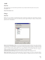
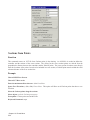
Store Project Archive . . . . . . . . . . . . . . . . . . . . . . . . . . . . . . . . . . . . . . . . . .
82
Extract Project Archive . . . . . . . . . . . . . . . . . . . . . . . . . . . . . . . . . . . . . . . . .
82
Import Xref to Current Drawing . . . . . . . . . . . . . . . . . . . . . . . . . . . . . . . . . . . .
83
Xref Manager . . . . . . . . . . . . . . . . . . . . . . . . . . . . . . . . . . . . . . . . . . . . . .
83
Import-Export . . . . . . . . . . . . . . . . . . . . . . . . . . . . . . . . . . . . . . . . . . . . . .
85
Data Collectors . . . . . . . . . . . . . . . . . . . . . . . . . . . . . . . . . . . . . . . . .
85
Convert LDD-AEC Contours . . . . . . . . . . . . . . . . . . . . . . . . . . . . . . . . . . 108
Import/Export LandXML Files . . . . . . . . . . . . . . . . . . . . . . . . . . . . . . . . . 109
iii
Import/Export Carlson Triangulation Files . . . . . . . . . . . . . . . . . . . . . . . . . . . 110
Import/Export DXF Files . . . . . . . . . . . . . . . . . . . . . . . . . . . . . . . . . . . . 111
Import Polyline File . . . . . . . . . . . . . . . . . . . . . . . . . . . . . . . . . . . . . . 111
Export Polyline File . . . . . . . . . . . . . . . . . . . . . . . . . . . . . . . . . . . . . . 112
Export Surface DXF Files . . . . . . . . . . . . . . . . . . . . . . . . . . . . . . . . . . . 113
Export Topcon Tin File . . . . . . . . . . . . . . . . . . . . . . . . . . . . . . . . . . . . . 113
Clipboard . . . . . . . . . . . . . . . . . . . . . . . . . . . . . . . . . . . . . . . . . . . . . . . . 116
Display Last Report . . . . . . . . . . . . . . . . . . . . . . . . . . . . . . . . . . . . . . . . . . . 118
Exit . . . . . . . . . . . . . . . . . . . . . . . . . . . . . . . . . . . . . . . . . . . . . . . . . . . 118
Chapter 4.
Tools Menu
119
Drawing Cleanup . . . . . . . . . . . . . . . . . . . . . . . . . . . . . . . . . . . . . . . . . . . . 120
Define Layer Target/Material/Subgrade
. . . . . . . . . . . . . . . . . . . . . . . . . . . . . . . . 123
Edit Selected Layer . . . . . . . . . . . . . . . . . . . . . . . . . . . . . . . . . . . . . . . . . . . 126
Set Layer For Existing . . . . . . . . . . . . . . . . . . . . . . . . . . . . . . . . . . . . . . . . . 126
Set Layer For Design . . . . . . . . . . . . . . . . . . . . . . . . . . . . . . . . . . . . . . . . . . 127
Set Layer For Other . . . . . . . . . . . . . . . . . . . . . . . . . . . . . . . . . . . . . . . . . . . 127
Boundary Polyline . . . . . . . . . . . . . . . . . . . . . . . . . . . . . . . . . . . . . . . . . . . 127
Areas Of Interest . . . . . . . . . . . . . . . . . . . . . . . . . . . . . . . . . . . . . . . . . . . . 128
Topsoil Removal and Replament Options . . . . . . . . . . . . . . . . . . . . . . . . . . . . . . . 130
Make Existing Ground Surface . . . . . . . . . . . . . . . . . . . . . . . . . . . . . . . . . . . . . 134
Make Design Surface . . . . . . . . . . . . . . . . . . . . . . . . . . . . . . . . . . . . . . . . . . 136
Adjust Design Surface . . . . . . . . . . . . . . . . . . . . . . . . . . . . . . . . . . . . . . . . . 137
Overexcavate Surface . . . . . . . . . . . . . . . . . . . . . . . . . . . . . . . . . . . . . . . . . . 137
Make Overexcavation Surface From Exsting/Design Surface . . . . . . . . . . . . . . . . . 137
Make Overexcavation Surface From Strata Surface . . . . . . . . . . . . . . . . . . . . . . 138
Make Overexcavate Surface From Screen Entities . . . . . . . . . . . . . . . . . . . . . . . 138
Adjust Overexcavate Surface . . . . . . . . . . . . . . . . . . . . . . . . . . . . . . . . . . 139
View Overexcavate Surface . . . . . . . . . . . . . . . . . . . . . . . . . . . . . . . . . . 139
Draw Overexcavate Surface 3D Faces . . . . . . . . . . . . . . . . . . . . . . . . . . . . . 139
Erase Overexcavate Surface 3D Faces . . . . . . . . . . . . . . . . . . . . . . . . . . . . . 140
Draw Overexcavate Cut Color Map . . . . . . . . . . . . . . . . . . . . . . . . . . . . . . 140
Erase Overexcavate Cut Color Map . . . . . . . . . . . . . . . . . . . . . . . . . . . . . . 140
Clear Overexcavate Surface . . . . . . . . . . . . . . . . . . . . . . . . . . . . . . . . . . 140
Surface Manager . . . . . . . . . . . . . . . . . . . . . . . . . . . . . . . . . . . . . . . . . . . . 141
Make User-Defined Surface . . . . . . . . . . . . . . . . . . . . . . . . . . . . . . . . . . . . . . . 142
Contents
iv
Set Active Surfaces . . . . . . . . . . . . . . . . . . . . . . . . . . . . . . . . . . . . . . . . . . . 142
Design Surface Vertical Offset . . . . . . . . . . . . . . . . . . . . . . . . . . . . . . . . . . . . . 143
Existing Surface Vertical Offset
. . . . . . . . . . . . . . . . . . . . . . . . . . . . . . . . . . . . 143
Merge Existing With Design . . . . . . . . . . . . . . . . . . . . . . . . . . . . . . . . . . . . . . 143
Triangulate & Contour . . . . . . . . . . . . . . . . . . . . . . . . . . . . . . . . . . . . . . . . . 144
Triangulation File Utilities . . . . . . . . . . . . . . . . . . . . . . . . . . . . . . . . . . . . . . . 153
Volumes By Triangulation . . . . . . . . . . . . . . . . . . . . . . . . . . . . . . . . . . . . . . . 157
Draw 3DPoly Perimeter . . . . . . . . . . . . . . . . . . . . . . . . . . . . . . . . . . . . . . . . . 158
Draw 3DPoly Base Breakline . . . . . . . . . . . . . . . . . . . . . . . . . . . . . . . . . . . . . . 159
Calculate Stockpile Volume . . . . . . . . . . . . . . . . . . . . . . . . . . . . . . . . . . . . . . . 159
Calculate Pond/Pit Volume . . . . . . . . . . . . . . . . . . . . . . . . . . . . . . . . . . . . . . . 161
Calculate Total Volumes . . . . . . . . . . . . . . . . . . . . . . . . . . . . . . . . . . . . . . . . 162
Calculate Volumes Inside Perimeter . . . . . . . . . . . . . . . . . . . . . . . . . . . . . . . . . . 168
Material Quantities . . . . . . . . . . . . . . . . . . . . . . . . . . . . . . . . . . . . . . . . . . . 168
Chapter 5.
Edit Menu
177
Undo . . . . . . . . . . . . . . . . . . . . . . . . . . . . . . . . . . . . . . . . . . . . . . . . . . 178
Redo . . . . . . . . . . . . . . . . . . . . . . . . . . . . . . . . . . . . . . . . . . . . . . . . . . . 178
Erase, Select . . . . . . . . . . . . . . . . . . . . . . . . . . . . . . . . . . . . . . . . . . . . . . . 178
Erase by Layer . . . . . . . . . . . . . . . . . . . . . . . . . . . . . . . . . . . . . . . . . . . . . 178
Erase by Closed Polyline . . . . . . . . . . . . . . . . . . . . . . . . . . . . . . . . . . . . . . . . 179
Erase Outside . . . . . . . . . . . . . . . . . . . . . . . . . . . . . . . . . . . . . . . . . . . . . . 180
Move . . . . . . . . . . . . . . . . . . . . . . . . . . . . . . . . . . . . . . . . . . . . . . . . . . 180
Standard Copy
. . . . . . . . . . . . . . . . . . . . . . . . . . . . . . . . . . . . . . . . . . . . . 180
Copy To Layer . . . . . . . . . . . . . . . . . . . . . . . . . . . . . . . . . . . . . . . . . . . . . 180
Standard Explode . . . . . . . . . . . . . . . . . . . . . . . . . . . . . . . . . . . . . . . . . . . . 181
Block Explode
. . . . . . . . . . . . . . . . . . . . . . . . . . . . . . . . . . . . . . . . . . . . . 182
Align . . . . . . . . . . . . . . . . . . . . . . . . . . . . . . . . . . . . . . . . . . . . . . . . . . 182
2D Align . . . . . . . . . . . . . . . . . . . . . . . . . . . . . . . . . . . . . . . . . . . . . . . . 183
Trim . . . . . . . . . . . . . . . . . . . . . . . . . . . . . . . . . . . . . . . . . . . . . . . . . . . 183
Scale . . . . . . . . . . . . . . . . . . . . . . . . . . . . . . . . . . . . . . . . . . . . . . . . . . . 184
Extend To Edge . . . . . . . . . . . . . . . . . . . . . . . . . . . . . . . . . . . . . . . . . . . . . 184
Extend by Distance . . . . . . . . . . . . . . . . . . . . . . . . . . . . . . . . . . . . . . . . . . . 185
Break by Closed Polyline . . . . . . . . . . . . . . . . . . . . . . . . . . . . . . . . . . . . . . . . 186
Break At Selected Point . . . . . . . . . . . . . . . . . . . . . . . . . . . . . . . . . . . . . . . . . 187
Break Polyline at Specified Distances . . . . . . . . . . . . . . . . . . . . . . . . . . . . . . . . . 187
Contents
v
Break at Intersection . . . . . . . . . . . . . . . . . . . . . . . . . . . . . . . . . . . . . . . . . . 187
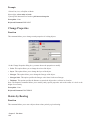
Change Properties . . . . . . . . . . . . . . . . . . . . . . . . . . . . . . . . . . . . . . . . . . . . 188
Rotate by Bearing . . . . . . . . . . . . . . . . . . . . . . . . . . . . . . . . . . . . . . . . . . . . 188
Standard Rotate . . . . . . . . . . . . . . . . . . . . . . . . . . . . . . . . . . . . . . . . . . . . . 189
Edit Text . . . . . . . . . . . . . . . . . . . . . . . . . . . . . . . . . . . . . . . . . . . . . . . . . 189
Find and Replace Text . . . . . . . . . . . . . . . . . . . . . . . . . . . . . . . . . . . . . . . . . 189
Text EnlargeReduce . . . . . . . . . . . . . . . . . . . . . . . . . . . . . . . . . . . . . . . . . . . 190
Text Explode To Polylines . . . . . . . . . . . . . . . . . . . . . . . . . . . . . . . . . . . . . . . 190
Image Frame . . . . . . . . . . . . . . . . . . . . . . . . . . . . . . . . . . . . . . . . . . . . . . 191
Image Clip . . . . . . . . . . . . . . . . . . . . . . . . . . . . . . . . . . . . . . . . . . . . . . . 191
Image Adjust . . . . . . . . . . . . . . . . . . . . . . . . . . . . . . . . . . . . . . . . . . . . . . 192
Remove Groups . . . . . . . . . . . . . . . . . . . . . . . . . . . . . . . . . . . . . . . . . . . . . 193
Join Nearest . . . . . . . . . . . . . . . . . . . . . . . . . . . . . . . . . . . . . . . . . . . . . . . 193
Offset Polyline . . . . . . . . . . . . . . . . . . . . . . . . . . . . . . . . . . . . . . . . . . . . . 194
Perimeter Polylines Properties . . . . . . . . . . . . . . . . . . . . . . . . . . . . . . . . . . . . . 195
3D Entity to 2D . . . . . . . . . . . . . . . . . . . . . . . . . . . . . . . . . . . . . . . . . . . . . 195
Perimeter Polylines Properties . . . . . . . . . . . . . . . . . . . . . . . . . . . . . . . . . . . . . 196
Entities to Polylines . . . . . . . . . . . . . . . . . . . . . . . . . . . . . . . . . . . . . . . . . . . 196
Reverse Polyline . . . . . . . . . . . . . . . . . . . . . . . . . . . . . . . . . . . . . . . . . . . . 197
Reduce Polyline Vertices . . . . . . . . . . . . . . . . . . . . . . . . . . . . . . . . . . . . . . . . 197
Densify Polyline Vertices . . . . . . . . . . . . . . . . . . . . . . . . . . . . . . . . . . . . . . . . 198
Draw Polyline Blips . . . . . . . . . . . . . . . . . . . . . . . . . . . . . . . . . . . . . . . . . . . 198
Set Polyline Origin . . . . . . . . . . . . . . . . . . . . . . . . . . . . . . . . . . . . . . . . . . . 199
Add Intersection Points . . . . . . . . . . . . . . . . . . . . . . . . . . . . . . . . . . . . . . . . . 199
Add Polyline Vertex . . . . . . . . . . . . . . . . . . . . . . . . . . . . . . . . . . . . . . . . . . . 199
Edit Polyline Vertex . . . . . . . . . . . . . . . . . . . . . . . . . . . . . . . . . . . . . . . . . . . 200
Edit Polyline Section . . . . . . . . . . . . . . . . . . . . . . . . . . . . . . . . . . . . . . . . . . 200
Remove Duplicate Polylines . . . . . . . . . . . . . . . . . . . . . . . . . . . . . . . . . . . . . . 202
Remove Polyline Arcs . . . . . . . . . . . . . . . . . . . . . . . . . . . . . . . . . . . . . . . . . 202
Remove Polyline Segment . . . . . . . . . . . . . . . . . . . . . . . . . . . . . . . . . . . . . . . 202
Remove Polyline Vertex . . . . . . . . . . . . . . . . . . . . . . . . . . . . . . . . . . . . . . . . 203
Break 3D Polyline by Surface . . . . . . . . . . . . . . . . . . . . . . . . . . . . . . . . . . . . . 203
Tag Hard Breakline Polylines . . . . . . . . . . . . . . . . . . . . . . . . . . . . . . . . . . . . . . 203
Untag Hard Breakline Polylines . . . . . . . . . . . . . . . . . . . . . . . . . . . . . . . . . . . . 204
Smooth Polyline . . . . . . . . . . . . . . . . . . . . . . . . . . . . . . . . . . . . . . . . . . . . . 204
Change Polyline Width . . . . . . . . . . . . . . . . . . . . . . . . . . . . . . . . . . . . . . . . . 205
Contents
vi
Check Elevation Range . . . . . . . . . . . . . . . . . . . . . . . . . . . . . . . . . . . . . . . . . 205
Close Polylines . . . . . . . . . . . . . . . . . . . . . . . . . . . . . . . . . . . . . . . . . . . . . 206
Open Polylines . . . . . . . . . . . . . . . . . . . . . . . . . . . . . . . . . . . . . . . . . . . . . 206
Highlight Crossing Plines . . . . . . . . . . . . . . . . . . . . . . . . . . . . . . . . . . . . . . . . 206
Select by Filter . . . . . . . . . . . . . . . . . . . . . . . . . . . . . . . . . . . . . . . . . . . . . 208
Select by Elevation . . . . . . . . . . . . . . . . . . . . . . . . . . . . . . . . . . . . . . . . . . . 208
Select by Area . . . . . . . . . . . . . . . . . . . . . . . . . . . . . . . . . . . . . . . . . . . . . . 209
Chapter 6.
View Menu
211
Redraw . . . . . . . . . . . . . . . . . . . . . . . . . . . . . . . . . . . . . . . . . . . . . . . . . 212
Regenerate
. . . . . . . . . . . . . . . . . . . . . . . . . . . . . . . . . . . . . . . . . . . . . . . 212
Zoom - Window . . . . . . . . . . . . . . . . . . . . . . . . . . . . . . . . . . . . . . . . . . . . . 212
Zoom - Dynamic . . . . . . . . . . . . . . . . . . . . . . . . . . . . . . . . . . . . . . . . . . . . 212
Zoom - Previous . . . . . . . . . . . . . . . . . . . . . . . . . . . . . . . . . . . . . . . . . . . . . 212
Zoom - Center . . . . . . . . . . . . . . . . . . . . . . . . . . . . . . . . . . . . . . . . . . . . . . 213
Zoom - Extents . . . . . . . . . . . . . . . . . . . . . . . . . . . . . . . . . . . . . . . . . . . . . 213
Zoom IN . . . . . . . . . . . . . . . . . . . . . . . . . . . . . . . . . . . . . . . . . . . . . . . . . 213
Zoom OUT . . . . . . . . . . . . . . . . . . . . . . . . . . . . . . . . . . . . . . . . . . . . . . . 213
Zoom Point(s) . . . . . . . . . . . . . . . . . . . . . . . . . . . . . . . . . . . . . . . . . . . . . . 214
Pan . . . . . . . . . . . . . . . . . . . . . . . . . . . . . . . . . . . . . . . . . . . . . . . . . . . 214
Twist Screen Standard
. . . . . . . . . . . . . . . . . . . . . . . . . . . . . . . . . . . . . . . . . 214
Twist Screen Line . . . . . . . . . . . . . . . . . . . . . . . . . . . . . . . . . . . . . . . . . . . . 215
Twist Screen Surveyor . . . . . . . . . . . . . . . . . . . . . . . . . . . . . . . . . . . . . . . . . 215
Restore Due North . . . . . . . . . . . . . . . . . . . . . . . . . . . . . . . . . . . . . . . . . . . 215
Display Order . . . . . . . . . . . . . . . . . . . . . . . . . . . . . . . . . . . . . . . . . . . . . . 215
Update Colors For Set Elevations . . . . . . . . . . . . . . . . . . . . . . . . . . . . . . . . . . . . 216
3D Drive Simutation . . . . . . . . . . . . . . . . . . . . . . . . . . . . . . . . . . . . . . . . . . 216
Existing Surface 3D Viewer . . . . . . . . . . . . . . . . . . . . . . . . . . . . . . . . . . . . . . 218
Design Surface 3D Viewer . . . . . . . . . . . . . . . . . . . . . . . . . . . . . . . . . . . . . . . 219
FlyOver Along 3D Polyline . . . . . . . . . . . . . . . . . . . . . . . . . . . . . . . . . . . . . . . 221
3D Viewer Window . . . . . . . . . . . . . . . . . . . . . . . . . . . . . . . . . . . . . . . . . . . 223
Viewpoint 3D . . . . . . . . . . . . . . . . . . . . . . . . . . . . . . . . . . . . . . . . . . . . . . 225
Layer Control . . . . . . . . . . . . . . . . . . . . . . . . . . . . . . . . . . . . . . . . . . . . . . 226
Change Layer . . . . . . . . . . . . . . . . . . . . . . . . . . . . . . . . . . . . . . . . . . . . . . 228
Freeze Layer . . . . . . . . . . . . . . . . . . . . . . . . . . . . . . . . . . . . . . . . . . . . . . 229
Thaw Layer . . . . . . . . . . . . . . . . . . . . . . . . . . . . . . . . . . . . . . . . . . . . . . . 229
Contents
vii
Isolate Layer . . . . . . . . . . . . . . . . . . . . . . . . . . . . . . . . . . . . . . . . . . . . . . 229
Restore Layer . . . . . . . . . . . . . . . . . . . . . . . . . . . . . . . . . . . . . . . . . . . . . . 229
Set Layer . . . . . . . . . . . . . . . . . . . . . . . . . . . . . . . . . . . . . . . . . . . . . . . . 229
Chapter 7.
Draw Menu
231
Line . . . . . . . . . . . . . . . . . . . . . . . . . . . . . . . . . . . . . . . . . . . . . . . . . . . 232
2D Polyline . . . . . . . . . . . . . . . . . . . . . . . . . . . . . . . . . . . . . . . . . . . . . . . 232
3D Polyline . . . . . . . . . . . . . . . . . . . . . . . . . . . . . . . . . . . . . . . . . . . . . . . 234
Circle . . . . . . . . . . . . . . . . . . . . . . . . . . . . . . . . . . . . . . . . . . . . . . . . . . 235
Insert Symbols . . . . . . . . . . . . . . . . . . . . . . . . . . . . . . . . . . . . . . . . . . . . . 235
Insert Drawing . . . . . . . . . . . . . . . . . . . . . . . . . . . . . . . . . . . . . . . . . . . . . 237
Write Block . . . . . . . . . . . . . . . . . . . . . . . . . . . . . . . . . . . . . . . . . . . . . . . 238
Text . . . . . . . . . . . . . . . . . . . . . . . . . . . . . . . . . . . . . . . . . . . . . . . . . . . 240
Hatch . . . . . . . . . . . . . . . . . . . . . . . . . . . . . . . . . . . . . . . . . . . . . . . . . . 241
2 Tangents Radius . . . . . . . . . . . . . . . . . . . . . . . . . . . . . . . . . . . . . . . . . . . . 244
2 Tangents Arc Length . . . . . . . . . . . . . . . . . . . . . . . . . . . . . . . . . . . . . . . . . 245
2 Tangents Chord Length . . . . . . . . . . . . . . . . . . . . . . . . . . . . . . . . . . . . . . . . 245
3 Point Curve . . . . . . . . . . . . . . . . . . . . . . . . . . . . . . . . . . . . . . . . . . . . . . 245
PC PT Radius Point . . . . . . . . . . . . . . . . . . . . . . . . . . . . . . . . . . . . . . . . . . . 246
PC Radius Chord . . . . . . . . . . . . . . . . . . . . . . . . . . . . . . . . . . . . . . . . . . . . 246
Raster Image . . . . . . . . . . . . . . . . . . . . . . . . . . . . . . . . . . . . . . . . . . . . . . 247
Place Image by World File . . . . . . . . . . . . . . . . . . . . . . . . . . . . . . . . . . . . . . . 249
Closed Polyline By Interior Point . . . . . . . . . . . . . . . . . . . . . . . . . . . . . . . . . . . . 249
ShrinkWrap Entities . . . . . . . . . . . . . . . . . . . . . . . . . . . . . . . . . . . . . . . . . . . 250
Building Envelope Polyline . . . . . . . . . . . . . . . . . . . . . . . . . . . . . . . . . . . . . . . 251
Design Pad Template . . . . . . . . . . . . . . . . . . . . . . . . . . . . . . . . . . . . . . . . . . 252
Title Block . . . . . . . . . . . . . . . . . . . . . . . . . . . . . . . . . . . . . . . . . . . . . . . 260
Distance with Leader . . . . . . . . . . . . . . . . . . . . . . . . . . . . . . . . . . . . . . . . . . 262
Curve Arrow . . . . . . . . . . . . . . . . . . . . . . . . . . . . . . . . . . . . . . . . . . . . . . 262
Bar Scale . . . . . . . . . . . . . . . . . . . . . . . . . . . . . . . . . . . . . . . . . . . . . . . . 263
North Arrow . . . . . . . . . . . . . . . . . . . . . . . . . . . . . . . . . . . . . . . . . . . . . . . 263
Contour Elevation Label . . . . . . . . . . . . . . . . . . . . . . . . . . . . . . . . . . . . . . . . 264
Color Contours by Elevation . . . . . . . . . . . . . . . . . . . . . . . . . . . . . . . . . . . . . . 266
Color Contours by Interval . . . . . . . . . . . . . . . . . . . . . . . . . . . . . . . . . . . . . . . 267
Draw Triangular Surface . . . . . . . . . . . . . . . . . . . . . . . . . . . . . . . . . . . . . . . . 268
Run Off Tracking . . . . . . . . . . . . . . . . . . . . . . . . . . . . . . . . . . . . . . . . . . . . 269
Contents
viii
Slope At Point . . . . . . . . . . . . . . . . . . . . . . . . . . . . . . . . . . . . . . . . . . . . . 270
Cut Fill Map Legend . . . . . . . . . . . . . . . . . . . . . . . . . . . . . . . . . . . . . . . . . . 271
Cut Fill Labels . . . . . . . . . . . . . . . . . . . . . . . . . . . . . . . . . . . . . . . . . . . . . 271
Cut Fill Centroids . . . . . . . . . . . . . . . . . . . . . . . . . . . . . . . . . . . . . . . . . . . . 273
Point Defaults . . . . . . . . . . . . . . . . . . . . . . . . . . . . . . . . . . . . . . . . . . . . . . 275
Draw-Locate Points . . . . . . . . . . . . . . . . . . . . . . . . . . . . . . . . . . . . . . . . . . . 277
Field to Finish . . . . . . . . . . . . . . . . . . . . . . . . . . . . . . . . . . . . . . . . . . . . . . 280
Spreadsheet Edit Points . . . . . . . . . . . . . . . . . . . . . . . . . . . . . . . . . . . . . . . . . 296
On-Screen Edit Points . . . . . . . . . . . . . . . . . . . . . . . . . . . . . . . . . . . . . . . . . . 297
Scale Point Attributes
. . . . . . . . . . . . . . . . . . . . . . . . . . . . . . . . . . . . . . . . . 297
Resize Point Attributes . . . . . . . . . . . . . . . . . . . . . . . . . . . . . . . . . . . . . . . . . 298
Twist Point Attributes . . . . . . . . . . . . . . . . . . . . . . . . . . . . . . . . . . . . . . . . . . 298
Erase Points . . . . . . . . . . . . . . . . . . . . . . . . . . . . . . . . . . . . . . . . . . . . . . . 299
Create Points from Entities . . . . . . . . . . . . . . . . . . . . . . . . . . . . . . . . . . . . . . . 300
Coordinate File Utilities
. . . . . . . . . . . . . . . . . . . . . . . . . . . . . . . . . . . . . . . . 301
Point Group Manager . . . . . . . . . . . . . . . . . . . . . . . . . . . . . . . . . . . . . . . . . . 308
Interpolate Points . . . . . . . . . . . . . . . . . . . . . . . . . . . . . . . . . . . . . . . . . . . . 316
Spot Elevation . . . . . . . . . . . . . . . . . . . . . . . . . . . . . . . . . . . . . . . . . . . . . 318
Create Points On Surface . . . . . . . . . . . . . . . . . . . . . . . . . . . . . . . . . . . . . . . . 319
Set Point Elevations To Surface . . . . . . . . . . . . . . . . . . . . . . . . . . . . . . . . . . . . . 320
Import Text/ASCII File . . . . . . . . . . . . . . . . . . . . . . . . . . . . . . . . . . . . . . . . . 321
Import TDS RD5 File . . . . . . . . . . . . . . . . . . . . . . . . . . . . . . . . . . . . . . . . . . 323
Import LDD MDB File . . . . . . . . . . . . . . . . . . . . . . . . . . . . . . . . . . . . . . . . . 323
Export Text/ASCII File . . . . . . . . . . . . . . . . . . . . . . . . . . . . . . . . . . . . . . . . . 323
Convert Points to AECC POINTs . . . . . . . . . . . . . . . . . . . . . . . . . . . . . . . . . . . . 325
Convert Points to Softdesk . . . . . . . . . . . . . . . . . . . . . . . . . . . . . . . . . . . . . . . 325
Convert Points to C&G . . . . . . . . . . . . . . . . . . . . . . . . . . . . . . . . . . . . . . . . . 325
Convert Wild/Leica to Points . . . . . . . . . . . . . . . . . . . . . . . . . . . . . . . . . . . . . . 326
Convert Points to Eagle Point . . . . . . . . . . . . . . . . . . . . . . . . . . . . . . . . . . . . . . 326
Chapter 8.
Digitize Menu
327
Digitizer Setup . . . . . . . . . . . . . . . . . . . . . . . . . . . . . . . . . . . . . . . . . . . . . 328
Tablet On . . . . . . . . . . . . . . . . . . . . . . . . . . . . . . . . . . . . . . . . . . . . . . . . 329
Tablet Off . . . . . . . . . . . . . . . . . . . . . . . . . . . . . . . . . . . . . . . . . . . . . . . . 329
Tablet Calibrate . . . . . . . . . . . . . . . . . . . . . . . . . . . . . . . . . . . . . . . . . . . . . 330
Save Tablet Calibration . . . . . . . . . . . . . . . . . . . . . . . . . . . . . . . . . . . . . . . . . 332
Contents
ix
Load Tablet Calibration . . . . . . . . . . . . . . . . . . . . . . . . . . . . . . . . . . . . . . . . . 332
Digitizer Settings . . . . . . . . . . . . . . . . . . . . . . . . . . . . . . . . . . . . . . . . . . . . 332
Existing . . . . . . . . . . . . . . . . . . . . . . . . . . . . . . . . . . . . . . . . . . . . . . . . . 334
Design . . . . . . . . . . . . . . . . . . . . . . . . . . . . . . . . . . . . . . . . . . . . . . . . . . 334
Other . . . . . . . . . . . . . . . . . . . . . . . . . . . . . . . . . . . . . . . . . . . . . . . . . . 334
Point . . . . . . . . . . . . . . . . . . . . . . . . . . . . . . . . . . . . . . . . . . . . . . . . . . . 334
Spot Elevation . . . . . . . . . . . . . . . . . . . . . . . . . . . . . . . . . . . . . . . . . . . . . . 335
2D Polyline . . . . . . . . . . . . . . . . . . . . . . . . . . . . . . . . . . . . . . . . . . . . . . . 337
3D Polyline . . . . . . . . . . . . . . . . . . . . . . . . . . . . . . . . . . . . . . . . . . . . . . . 338
Perimeter . . . . . . . . . . . . . . . . . . . . . . . . . . . . . . . . . . . . . . . . . . . . . . . . 339
Areas . . . . . . . . . . . . . . . . . . . . . . . . . . . . . . . . . . . . . . . . . . . . . . . . . . 340
Contour Polyline . . . . . . . . . . . . . . . . . . . . . . . . . . . . . . . . . . . . . . . . . . . . 341
Sections . . . . . . . . . . . . . . . . . . . . . . . . . . . . . . . . . . . . . . . . . . . . . . . . . 342
End Areas . . . . . . . . . . . . . . . . . . . . . . . . . . . . . . . . . . . . . . . . . . . . . . . . 345
Chapter 9.
Elevate Menu
347
Change Elevations . . . . . . . . . . . . . . . . . . . . . . . . . . . . . . . . . . . . . . . . . . . 348
Set Polyline to Elevation . . . . . . . . . . . . . . . . . . . . . . . . . . . . . . . . . . . . . . . . 348
Edit-Assign Polyline to Elevations . . . . . . . . . . . . . . . . . . . . . . . . . . . . . . . . . . . 349
Edit Polyline Vertex . . . . . . . . . . . . . . . . . . . . . . . . . . . . . . . . . . . . . . . . . . . 350
2D to 3D Polyline by Points . . . . . . . . . . . . . . . . . . . . . . . . . . . . . . . . . . . . . . 351
2D to 3D Polyline-By Text . . . . . . . . . . . . . . . . . . . . . . . . . . . . . . . . . . . . . . . 352
2D to 3D-By Text With Leader . . . . . . . . . . . . . . . . . . . . . . . . . . . . . . . . . . . . . 353
2D to 3D Polyline by Start/End Elevations . . . . . . . . . . . . . . . . . . . . . . . . . . . . . . . 355
Pad Polyline By Interior Text . . . . . . . . . . . . . . . . . . . . . . . . . . . . . . . . . . . . . . 356
Drape 3D Polyline On Surface . . . . . . . . . . . . . . . . . . . . . . . . . . . . . . . . . . . . . 358
Convert Spot Elev To Points . . . . . . . . . . . . . . . . . . . . . . . . . . . . . . . . . . . . . . 359
Assign Contour Elevations - Multiple in Series . . . . . . . . . . . . . . . . . . . . . . . . . . . . 362
Assign Contour Elevations - From Contour Labels . . . . . . . . . . . . . . . . . . . . . . . . . . . 364
Assign Contour Elevations - Single Elevation Group
. . . . . . . . . . . . . . . . . . . . . . . . . 365
Edit Contours . . . . . . . . . . . . . . . . . . . . . . . . . . . . . . . . . . . . . . . . . . . . . . 365
Chapter 10.
Inquiry Menu
367
List . . . . . . . . . . . . . . . . . . . . . . . . . . . . . . . . . . . . . . . . . . . . . . . . . . . 368
Point ID . . . . . . . . . . . . . . . . . . . . . . . . . . . . . . . . . . . . . . . . . . . . . . . . . 369
Layer ID . . . . . . . . . . . . . . . . . . . . . . . . . . . . . . . . . . . . . . . . . . . . . . . . . 369
Contents
x
Curve Info . . . . . . . . . . . . . . . . . . . . . . . . . . . . . . . . . . . . . . . . . . . . . . . . 370
Polyline Info . . . . . . . . . . . . . . . . . . . . . . . . . . . . . . . . . . . . . . . . . . . . . . 370
Surface Inspector . . . . . . . . . . . . . . . . . . . . . . . . . . . . . . . . . . . . . . . . . . . . 370
Surface Report . . . . . . . . . . . . . . . . . . . . . . . . . . . . . . . . . . . . . . . . . . . . . 371
Drawing Inspector
. . . . . . . . . . . . . . . . . . . . . . . . . . . . . . . . . . . . . . . . . . . 372
Layer Inspector . . . . . . . . . . . . . . . . . . . . . . . . . . . . . . . . . . . . . . . . . . . . . 374
Layer Report . . . . . . . . . . . . . . . . . . . . . . . . . . . . . . . . . . . . . . . . . . . . . . 374
Hatch Subgrade Areas . . . . . . . . . . . . . . . . . . . . . . . . . . . . . . . . . . . . . . . . . 375
Erase Subgrade Hatches
. . . . . . . . . . . . . . . . . . . . . . . . . . . . . . . . . . . . . . . . 377
Hatch Subgrade Areas . . . . . . . . . . . . . . . . . . . . . . . . . . . . . . . . . . . . . . . . . 377
Label Subgrade Areas . . . . . . . . . . . . . . . . . . . . . . . . . . . . . . . . . . . . . . . . . . 378
Erase Subgrade Labels . . . . . . . . . . . . . . . . . . . . . . . . . . . . . . . . . . . . . . . . . 378
List Elevation . . . . . . . . . . . . . . . . . . . . . . . . . . . . . . . . . . . . . . . . . . . . . . 378
Distance Report . . . . . . . . . . . . . . . . . . . . . . . . . . . . . . . . . . . . . . . . . . . . . 379
Bearing and Distance . . . . . . . . . . . . . . . . . . . . . . . . . . . . . . . . . . . . . . . . . . 379
Label Angle . . . . . . . . . . . . . . . . . . . . . . . . . . . . . . . . . . . . . . . . . . . . . . . 379
Polyline Report . . . . . . . . . . . . . . . . . . . . . . . . . . . . . . . . . . . . . . . . . . . . . 380
Slope Report . . . . . . . . . . . . . . . . . . . . . . . . . . . . . . . . . . . . . . . . . . . . . . 382
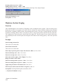
Slope Zone Analysis . . . . . . . . . . . . . . . . . . . . . . . . . . . . . . . . . . . . . . . . . . 383
Elevation Zone Analysis . . . . . . . . . . . . . . . . . . . . . . . . . . . . . . . . . . . . . . . . 387
Story Stake From Surface Entities . . . . . . . . . . . . . . . . . . . . . . . . . . . . . . . . . . . 390
Story Stake By Points/Polyline . . . . . . . . . . . . . . . . . . . . . . . . . . . . . . . . . . . . . 391
Area Defaults . . . . . . . . . . . . . . . . . . . . . . . . . . . . . . . . . . . . . . . . . . . . . . 392
Area by Inverse . . . . . . . . . . . . . . . . . . . . . . . . . . . . . . . . . . . . . . . . . . . . . 394
Area by Lines & Arcs . . . . . . . . . . . . . . . . . . . . . . . . . . . . . . . . . . . . . . . . . . 394
Area by Interior Point . . . . . . . . . . . . . . . . . . . . . . . . . . . . . . . . . . . . . . . . . . 395
Area by Closed Polylines . . . . . . . . . . . . . . . . . . . . . . . . . . . . . . . . . . . . . . . . 395
Area Descriptions . . . . . . . . . . . . . . . . . . . . . . . . . . . . . . . . . . . . . . . . . . . . 396
Chapter 11.
Settings Menu
399
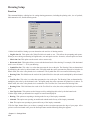
Drawing Setup . . . . . . . . . . . . . . . . . . . . . . . . . . . . . . . . . . . . . . . . . . . . . 400
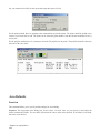
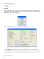
Preferences . . . . . . . . . . . . . . . . . . . . . . . . . . . . . . . . . . . . . . . . . . . . . . . 401
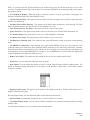
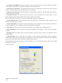
Configure . . . . . . . . . . . . . . . . . . . . . . . . . . . . . . . . . . . . . . . . . . . . . . . . 402
Edit Symbol Library . . . . . . . . . . . . . . . . . . . . . . . . . . . . . . . . . . . . . . . . . . 407
Toolbars . . . . . . . . . . . . . . . . . . . . . . . . . . . . . . . . . . . . . . . . . . . . . . . . . 408
Text Style . . . . . . . . . . . . . . . . . . . . . . . . . . . . . . . . . . . . . . . . . . . . . . . . 409
Contents
xi
Units Control . . . . . . . . . . . . . . . . . . . . . . . . . . . . . . . . . . . . . . . . . . . . . . 410
Object Snap . . . . . . . . . . . . . . . . . . . . . . . . . . . . . . . . . . . . . . . . . . . . . . . 412
Mouse Clicking Settings . . . . . . . . . . . . . . . . . . . . . . . . . . . . . . . . . . . . . . . . 415
Crosshairs . . . . . . . . . . . . . . . . . . . . . . . . . . . . . . . . . . . . . . . . . . . . . . . . 415
Set UCS to World . . . . . . . . . . . . . . . . . . . . . . . . . . . . . . . . . . . . . . . . . . . . 416
Set Environment Variables . . . . . . . . . . . . . . . . . . . . . . . . . . . . . . . . . . . . . . . 416
Chapter 12.
Drillhole Menu
419
Drillhole Strata Settings . . . . . . . . . . . . . . . . . . . . . . . . . . . . . . . . . . . . . . . . . 420
Drillhole Import . . . . . . . . . . . . . . . . . . . . . . . . . . . . . . . . . . . . . . . . . . . . . 422
Place Drillhole . . . . . . . . . . . . . . . . . . . . . . . . . . . . . . . . . . . . . . . . . . . . . 424
Edit Drillhole . . . . . . . . . . . . . . . . . . . . . . . . . . . . . . . . . . . . . . . . . . . . . . 426
Reports . . . . . . . . . . . . . . . . . . . . . . . . . . . . . . . . . . . . . . . . . . . . . . . . . 428
Make Strata Surface . . . . . . . . . . . . . . . . . . . . . . . . . . . . . . . . . . . . . . . . . . . 430
Clear Strata Surface . . . . . . . . . . . . . . . . . . . . . . . . . . . . . . . . . . . . . . . . . . . 430
Draw Strata Cut Depth Contours . . . . . . . . . . . . . . . . . . . . . . . . . . . . . . . . . . . . 431
Erase Strata Cut Depth Contours . . . . . . . . . . . . . . . . . . . . . . . . . . . . . . . . . . . . 431
Draw Strata Cut Color Map . . . . . . . . . . . . . . . . . . . . . . . . . . . . . . . . . . . . . . . 432
Erase Strata Cut Color Map . . . . . . . . . . . . . . . . . . . . . . . . . . . . . . . . . . . . . . . 432
Draw Strata Surface . . . . . . . . . . . . . . . . . . . . . . . . . . . . . . . . . . . . . . . . . . . 433
Erase Strata Surface . . . . . . . . . . . . . . . . . . . . . . . . . . . . . . . . . . . . . . . . . . . 433
Chapter 13.
Trench Menu
435
Input Trench From Polyline . . . . . . . . . . . . . . . . . . . . . . . . . . . . . . . . . . . . . . . 436
Create Trench Network Structure . . . . . . . . . . . . . . . . . . . . . . . . . . . . . . . . . . . . 437
Edit Trench Network Structure . . . . . . . . . . . . . . . . . . . . . . . . . . . . . . . . . . . . . 439
Remove Trench Network Structure . . . . . . . . . . . . . . . . . . . . . . . . . . . . . . . . . . . 440
Find Trench Network Structure . . . . . . . . . . . . . . . . . . . . . . . . . . . . . . . . . . . . . 441
Export Trench Network Data . . . . . . . . . . . . . . . . . . . . . . . . . . . . . . . . . . . . . . 441
Trench Network File Backup . . . . . . . . . . . . . . . . . . . . . . . . . . . . . . . . . . . . . . 442
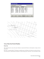
Draw Trench Network Plan View . . . . . . . . . . . . . . . . . . . . . . . . . . . . . . . . . . . . 442
Draw Trench Network Profile . . . . . . . . . . . . . . . . . . . . . . . . . . . . . . . . . . . . . . 442
Plain View Label Settings . . . . . . . . . . . . . . . . . . . . . . . . . . . . . . . . . . . . . . . . 446
Input Edit Trench Template . . . . . . . . . . . . . . . . . . . . . . . . . . . . . . . . . . . . . . . 448
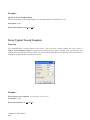
Draw Typical Trench Template . . . . . . . . . . . . . . . . . . . . . . . . . . . . . . . . . . . . . 450
Trench Subgrade Areas . . . . . . . . . . . . . . . . . . . . . . . . . . . . . . . . . . . . . . . . . 451
Contents
xii
Trench Network Quantities . . . . . . . . . . . . . . . . . . . . . . . . . . . . . . . . . . . . . . . 451
Report Trench Network . . . . . . . . . . . . . . . . . . . . . . . . . . . . . . . . . . . . . . . . . 453
Chapter 14.
Roads Menu
455
Input-Edit Centerline File . . . . . . . . . . . . . . . . . . . . . . . . . . . . . . . . . . . . . . . . 456
Polyline to Centerline File . . . . . . . . . . . . . . . . . . . . . . . . . . . . . . . . . . . . . . . 462
Draw Centerline File . . . . . . . . . . . . . . . . . . . . . . . . . . . . . . . . . . . . . . . . . . 462
Centerline Report . . . . . . . . . . . . . . . . . . . . . . . . . . . . . . . . . . . . . . . . . . . . 463
Import Centerline . . . . . . . . . . . . . . . . . . . . . . . . . . . . . . . . . . . . . . . . . . . . 464
Station Polyline/Centerline . . . . . . . . . . . . . . . . . . . . . . . . . . . . . . . . . . . . . . . 464
Label Station-Offset . . . . . . . . . . . . . . . . . . . . . . . . . . . . . . . . . . . . . . . . . . . 470
Offset Point Entry . . . . . . . . . . . . . . . . . . . . . . . . . . . . . . . . . . . . . . . . . . . . 473
Calculate Offsets . . . . . . . . . . . . . . . . . . . . . . . . . . . . . . . . . . . . . . . . . . . . 475
Quick Profile From Surfaces . . . . . . . . . . . . . . . . . . . . . . . . . . . . . . . . . . . . . . 477
Profile From Existing Surface
. . . . . . . . . . . . . . . . . . . . . . . . . . . . . . . . . . . . . 479
Profile from Design Surface . . . . . . . . . . . . . . . . . . . . . . . . . . . . . . . . . . . . . . 479
Design Road Profile . . . . . . . . . . . . . . . . . . . . . . . . . . . . . . . . . . . . . . . . . . . 480
Design Sewer/Pipe Profile . . . . . . . . . . . . . . . . . . . . . . . . . . . . . . . . . . . . . . . 482
Quick Profile from Screen Entities . . . . . . . . . . . . . . . . . . . . . . . . . . . . . . . . . . . 489
Profile from Screen Entities . . . . . . . . . . . . . . . . . . . . . . . . . . . . . . . . . . . . . . . 491
Profile from Grid or TIN File . . . . . . . . . . . . . . . . . . . . . . . . . . . . . . . . . . . . . . 492
Profile from 2D Polyline . . . . . . . . . . . . . . . . . . . . . . . . . . . . . . . . . . . . . . . . 492
Profile from 3D Polyline . . . . . . . . . . . . . . . . . . . . . . . . . . . . . . . . . . . . . . . . 493
Profile from Points on Centerline . . . . . . . . . . . . . . . . . . . . . . . . . . . . . . . . . . . . 493
Import Profile . . . . . . . . . . . . . . . . . . . . . . . . . . . . . . . . . . . . . . . . . . . . . . 494
Profile To 3D Polyline . . . . . . . . . . . . . . . . . . . . . . . . . . . . . . . . . . . . . . . . . 494
Profile To Points . . . . . . . . . . . . . . . . . . . . . . . . . . . . . . . . . . . . . . . . . . . . . 495
Input-Edit Profile File . . . . . . . . . . . . . . . . . . . . . . . . . . . . . . . . . . . . . . . . . . 497
Draw Profile . . . . . . . . . . . . . . . . . . . . . . . . . . . . . . . . . . . . . . . . . . . . . . . 499
Polyline Slope Report . . . . . . . . . . . . . . . . . . . . . . . . . . . . . . . . . . . . . . . . . . 507
Pipe Depth Summary . . . . . . . . . . . . . . . . . . . . . . . . . . . . . . . . . . . . . . . . . . 509
Profile Report . . . . . . . . . . . . . . . . . . . . . . . . . . . . . . . . . . . . . . . . . . . . . . 511
Quick Section . . . . . . . . . . . . . . . . . . . . . . . . . . . . . . . . . . . . . . . . . . . . . . 512
Input-Edit Section Alignment . . . . . . . . . . . . . . . . . . . . . . . . . . . . . . . . . . . . . . 515
Sections From Existing Surface . . . . . . . . . . . . . . . . . . . . . . . . . . . . . . . . . . . . . 517
Sections From Design Surface . . . . . . . . . . . . . . . . . . . . . . . . . . . . . . . . . . . . . 517
Contents
xiii
Sections from Screen Entities . . . . . . . . . . . . . . . . . . . . . . . . . . . . . . . . . . . . . . 518
Sections from Grid or TIN File . . . . . . . . . . . . . . . . . . . . . . . . . . . . . . . . . . . . . 520
Sections from Polylines . . . . . . . . . . . . . . . . . . . . . . . . . . . . . . . . . . . . . . . . . 520
Sections from Points . . . . . . . . . . . . . . . . . . . . . . . . . . . . . . . . . . . . . . . . . . 522
Import Sections . . . . . . . . . . . . . . . . . . . . . . . . . . . . . . . . . . . . . . . . . . . . . 523
Sections to 3D Polylines . . . . . . . . . . . . . . . . . . . . . . . . . . . . . . . . . . . . . . . . 523
Sections to Points . . . . . . . . . . . . . . . . . . . . . . . . . . . . . . . . . . . . . . . . . . . . 524
Slope Zone Section Analysis . . . . . . . . . . . . . . . . . . . . . . . . . . . . . . . . . . . . . . 525
Highway Section Staging . . . . . . . . . . . . . . . . . . . . . . . . . . . . . . . . . . . . . . . . 526
Input-Edit Section File . . . . . . . . . . . . . . . . . . . . . . . . . . . . . . . . . . . . . . . . . 527
Draw Section File . . . . . . . . . . . . . . . . . . . . . . . . . . . . . . . . . . . . . . . . . . . . 532
Section Report . . . . . . . . . . . . . . . . . . . . . . . . . . . . . . . . . . . . . . . . . . . . . 543
Calculate Sections Volume . . . . . . . . . . . . . . . . . . . . . . . . . . . . . . . . . . . . . . . 545
Mass Haul Analysis . . . . . . . . . . . . . . . . . . . . . . . . . . . . . . . . . . . . . . . . . . . 546
Calculate End Area . . . . . . . . . . . . . . . . . . . . . . . . . . . . . . . . . . . . . . . . . . . 548
Input Edit End Area File . . . . . . . . . . . . . . . . . . . . . . . . . . . . . . . . . . . . . . . . 549
Print Earthwork File Report . . . . . . . . . . . . . . . . . . . . . . . . . . . . . . . . . . . . . . . 550
Design Template . . . . . . . . . . . . . . . . . . . . . . . . . . . . . . . . . . . . . . . . . . . . 551
Draw Typical Template . . . . . . . . . . . . . . . . . . . . . . . . . . . . . . . . . . . . . . . . . 562
Template Transition . . . . . . . . . . . . . . . . . . . . . . . . . . . . . . . . . . . . . . . . . . . 564
Input-Edit Super Elevation . . . . . . . . . . . . . . . . . . . . . . . . . . . . . . . . . . . . . . . 567
Input-Edit Template Series . . . . . . . . . . . . . . . . . . . . . . . . . . . . . . . . . . . . . . . 569
Topsoil Removal/Replacement . . . . . . . . . . . . . . . . . . . . . . . . . . . . . . . . . . . . . 570
Assign Template Point Profile . . . . . . . . . . . . . . . . . . . . . . . . . . . . . . . . . . . . . 572
Assign Template Point Centerline . . . . . . . . . . . . . . . . . . . . . . . . . . . . . . . . . . . 573
Process Road Design . . . . . . . . . . . . . . . . . . . . . . . . . . . . . . . . . . . . . . . . . . 577
Chapter 15.
Display Menu
587
Existing Drawing . . . . . . . . . . . . . . . . . . . . . . . . . . . . . . . . . . . . . . . . . . . . 588
Existing Contours . . . . . . . . . . . . . . . . . . . . . . . . . . . . . . . . . . . . . . . . . . . . 588
Existing Surface . . . . . . . . . . . . . . . . . . . . . . . . . . . . . . . . . . . . . . . . . . . . . 589
Design Drawing . . . . . . . . . . . . . . . . . . . . . . . . . . . . . . . . . . . . . . . . . . . . . 590
Design Contours . . . . . . . . . . . . . . . . . . . . . . . . . . . . . . . . . . . . . . . . . . . . 590
Design Surface . . . . . . . . . . . . . . . . . . . . . . . . . . . . . . . . . . . . . . . . . . . . . 591
Cut Fill Contours . . . . . . . . . . . . . . . . . . . . . . . . . . . . . . . . . . . . . . . . . . . . 592
Cut Fill Labels . . . . . . . . . . . . . . . . . . . . . . . . . . . . . . . . . . . . . . . . . . . . . 592
Contents
xiv
Cut Fill Color Map . . . . . . . . . . . . . . . . . . . . . . . . . . . . . . . . . . . . . . . . . . . 593
Other Drawing . . . . . . . . . . . . . . . . . . . . . . . . . . . . . . . . . . . . . . . . . . . . . 594
Display Options . . . . . . . . . . . . . . . . . . . . . . . . . . . . . . . . . . . . . . . . . . . . . 595
Chapter 16.
Window Menu
603
Chapter 17.
Help Menu
605
Project Checklist . . . . . . . . . . . . . . . . . . . . . . . . . . . . . . . . . . . . . . . . . . . . 606
OnLine Help . . . . . . . . . . . . . . . . . . . . . . . . . . . . . . . . . . . . . . . . . . . . . . 606
Training Movies . . . . . . . . . . . . . . . . . . . . . . . . . . . . . . . . . . . . . . . . . . . . . 606
Carlson WebSite . . . . . . . . . . . . . . . . . . . . . . . . . . . . . . . . . . . . . . . . . . . . 606
About Carlson TakeOff . . . . . . . . . . . . . . . . . . . . . . . . . . . . . . . . . . . . . . . . . 607
Contents
xv
Contents
xvi
Tutorial
1
1
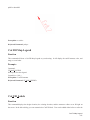
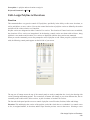
CAD File TakeOff
Note: Completing these tutorials will alter the drawing files (demo1.dwg, demo2.dwg, demo3.dwg). To run
through the tutorials a second time, copy over the original drawing files (.dwg) provided on the CD under
''Tutorials''. In addition, all demo .flt, .tin, .trg, .ini, .cl, .pro, .lot, .tpl, .bak, .sew, and .tch files need to be
deleted from the folder under C:\Program Files\Carlson TakeOff R1\WORK. If you have your own drawing
files, be sure to only delete files named demo1, demo2, or demo3, and not a file attached to one of your own drawing.
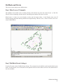
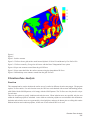
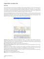
This lesson takes a drawing file from cleanup to volume calculations and surface viewing.
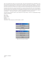
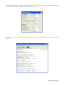
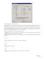
Step 1 (Start Takeoff):
Click the Windows icon for Takeoff to launch the program. You may be presented with a ''Startup Wizard'' dialog
and if so, click Exit.
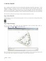
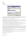
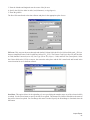
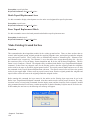
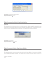
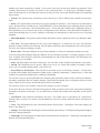
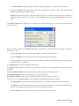
Step 2 (Open Drawing):
From the File menu, choose Open and select DEMO1.dwg from the TakeOff Work folder (ie.
C:\Program files\Carlson TakeOff R1\WORK\DEMO1.dwg).
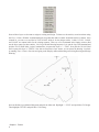
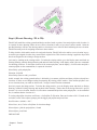
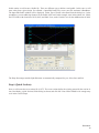
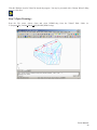
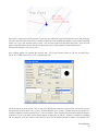
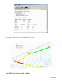
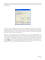
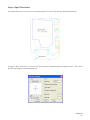
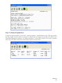
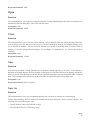
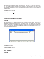
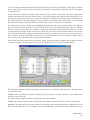
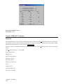
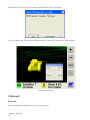
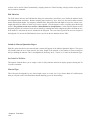
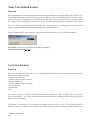
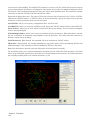
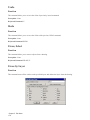
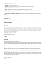
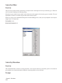
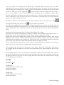
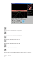
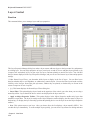
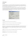
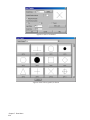
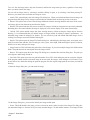
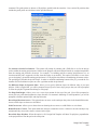
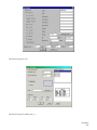
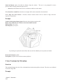
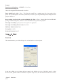
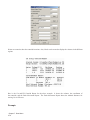
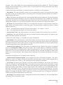
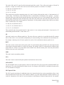
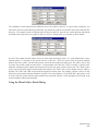
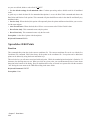
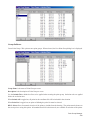
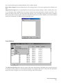
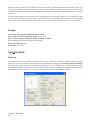
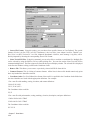
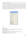
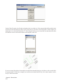
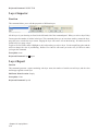
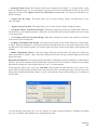
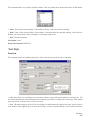
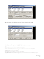
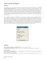
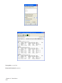
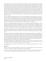
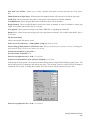
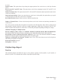
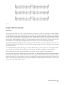
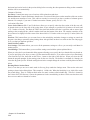
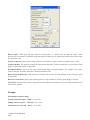
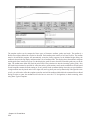
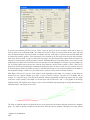
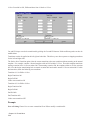
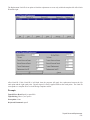
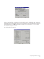
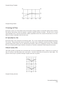
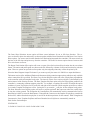
Now we can begin to process this drawing. The main TakeOff commands are listed in processing sequence in the
Tools menu. Many of these commands are also grouped as icons in the toolbar shown here.
Chapter 1. Tutorial
2
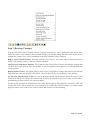
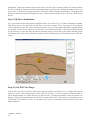
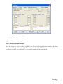
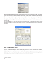
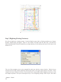
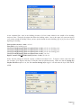
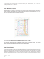
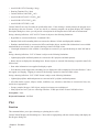
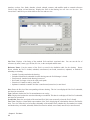
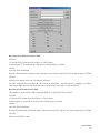
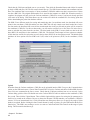
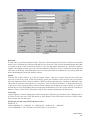
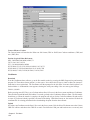
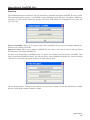
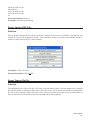
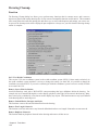
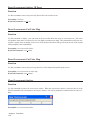
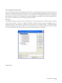
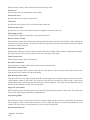
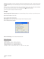
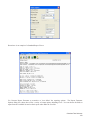
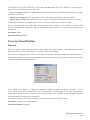
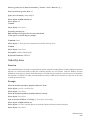
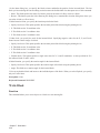
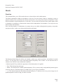
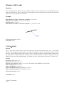
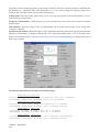
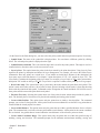
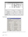
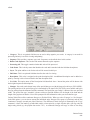
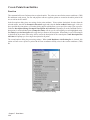
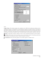
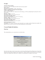
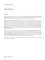
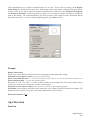
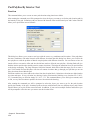
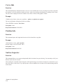
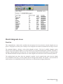
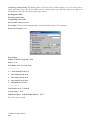
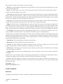
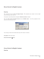
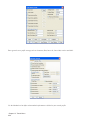
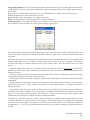
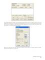
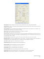
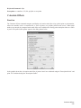
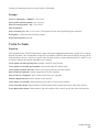
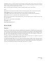
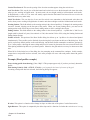
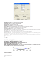
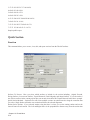
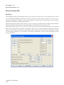
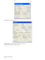
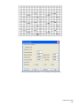
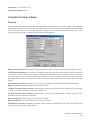
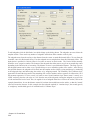
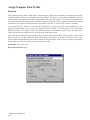
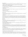
Step 3 (Drawing Cleanup):
From the Tools menu, choose Drawing Cleanup. Typically, drawings have lots of drafting fixes that must be done
before the surfaces can be modeled. This command will apply the selected cleanup functions on the drawing to help
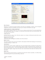
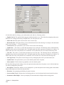
automate the cleanup. Here's a brief explaination of the most important of these functions:
Remove Layers With No Entities: Drawings often have lots of layers. This routine removes layers that have no
entities in the drawing so that we don't have to deal with them.
Join Linework With Same Endpoints: This routine will take linework that is broken into multiple segments and
join them into a single linework entity. For example, it will join together broken segments of a contour polyline into
a single polyline.
Reduce Polyline Vertices: This routine removes extra vertices from polylines as long as the removing does not shift
the polyline more than the specified Offset Cutoff. This will reduce the size and complexity of the drawing.
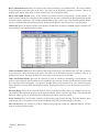
Set Elevation Outside Range To Zero: In case the drawing contains entities that are outside the range of valid
elevations for the site, this routine will set them to zero elevation. The program treats zero elevations as ''no elevation''
and modeling will filter out these zero elevation entities.
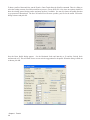
For this site, the elevations are around 800. So let's set the Min elevation to 500 and the Max elevation to 1000. The
cleanup will set any entities outside this elevation range to zero. With other TakeOff functions, we can later assign
proper elevations to any of these zero elevation entities that need to be used in modeling.
CAD File TakeOff
3
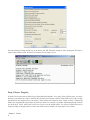
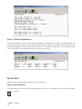
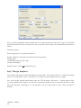
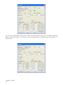
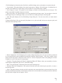
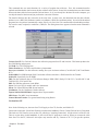
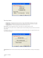
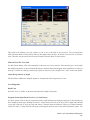
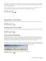
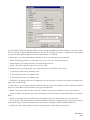
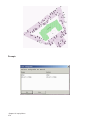
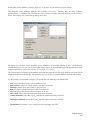
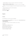
Once the Drawing Cleanup options are set as shown, pick OK. When the cleanup is done, the program will show a
report of the cleanup results. Pick the Exit button to exit the report viewer.
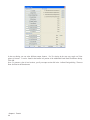
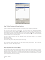
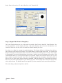
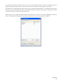
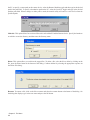
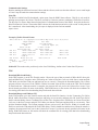
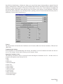
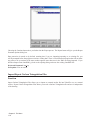
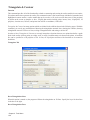
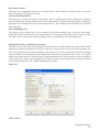
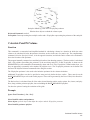
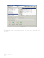
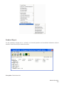
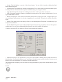
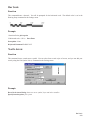
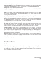
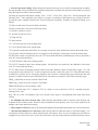
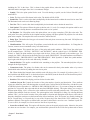
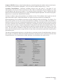
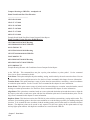
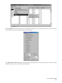
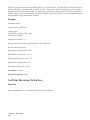
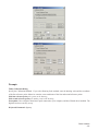
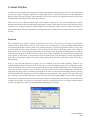
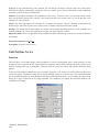
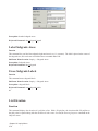
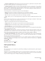
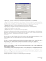
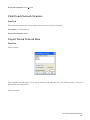
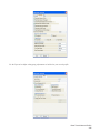
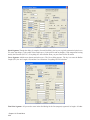
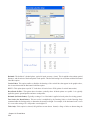
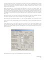
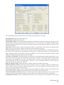
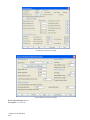
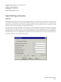
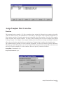
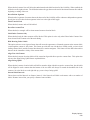
Step 4 (Layer Targets):
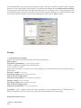
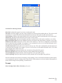
From the Tools menu, choose Define Layer Target/Material/Subgrade. Every entity (line, polyline, point, etc) in the
drawing is assigned a layer name. TakeOff uses the entity layer names to define which entities are for the existing
ground surface, the design surface or no surface. These surfaces are referred to as the ''Target'' surfaces. The drawing
entities are assigned their target surface by their layer name. For example, if polylines representing design contours
are on the layer ''Final'', then ''Final'' will be set as a layer for the design surface. For layers of entities that are for
neither existing nor design surfaces (such as text labels for street names), the layer target is set to Other.
Chapter 1. Tutorial
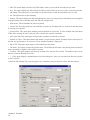
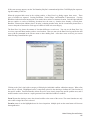
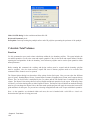
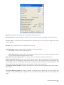
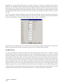
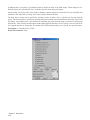
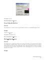
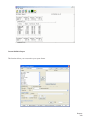
4
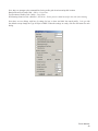
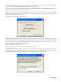
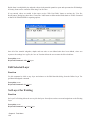
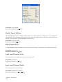
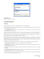
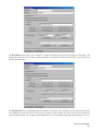
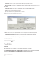
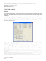
The Define Layer Targets dialog has three lists of layers: Existing, Design and Other. To switch between lists, pick
the tabs at the top of the dialog.
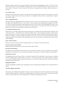
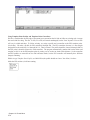
In this drawing, all the contours are for the existing ground surface. In the layer list, all the layers that start with
INDEX and INTER are for these contours. So highlight these layers and then choose Move To Existing. To highlight
multiple layers at a time, hold down the keyboard Ctrl key while picking with the mouse.
Next move the layer names that start with ''PR'' (for proposed) to the Design surface by highlighting these layers and
choosing Move To Design. Also move the layer ''PAD'' to design.
Next pick the Save button to save our changes and then pick Exit.
There are more tools for assigning layer targets. In the Display menu, you can turn on/off whether to display layer
targets by using Existing Drawing, Design Drawing and Other Drawing. For example, when Design Drawing is
checked, then picking this menu item will uncheck it and turn off all the layers for the design surface. Likewise,
picking Design Drawing when it is unchecked will make it checked and turn on the design surface layers.
Practice turning on/off the Existing, Design and Other Drawing in the Display menu. When only Existing Drawing
is on, you should see just the contours. When only Design Drawing is on, you should see just the design polylines
and leader labels. When only Other Drawing is on, you should see the entities that are assigned to neither existing
nor design.
CAD File TakeOff
5
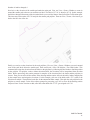
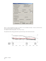
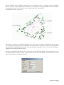
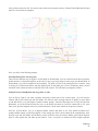
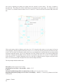
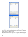
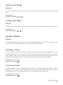
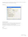
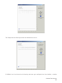
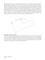
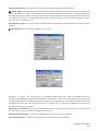
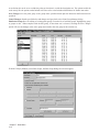
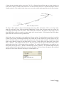
Some of these layers we do want to assign to existing and design. To better see the entities, zoom in on them using
the View->Zoom->Window command and pick two points that make a window around the entities as shown. Once
zoomed in, you can see a text label of ''818.70 PAD'' which is for the design surface. Labels ''817.00'', ''818.00''
and ''819.00'' are contour labels for the existing contours. There are a few commands in the Inquiry menu to find
out the layer names for these entities: List, Layer ID and Drawing Inspector. Let's run the Layer ID command and
pick the ''818.70 PAD'' label. At the Command line, it reports this layer is ''—-TX07''. Next pick the ''818.00'' label
and it reports this layer is ''TEXTS''. Now that we know these layer names, we can return the drawing view back
by running View->Zoom->Previous and going to the Display menu and checking on Existing Drawing and Design
Drawing.
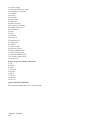
Next run Define Layer/Material/Subgrade and pick the Other tab. Highlight ''—-TX07'' and pick Move To Design.
Then highlight ''TEXTS'' and pick Move To Existing.
Chapter 1. Tutorial
6
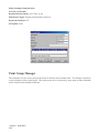
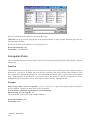
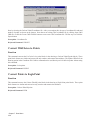
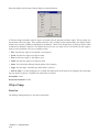
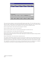
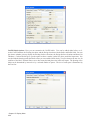
CAD File TakeOff
7
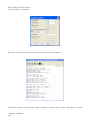
Check that your Layer Targets match the three lists shown here. Then pick Save and Exit.
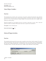
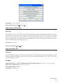
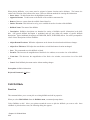
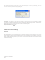
Step 5 (Define Material/SubGrade):
Besides assigning target surfaces by layer, layers are also used to define material names and subgrades depths. By
assigning material names and depths to layers, the volume, area, length and count for entities on these layers can be
reported. Also the depth is used to vertically adjust the design surface. The polylines used for subgrade depth must
be closed polylines. TakeOff supports nested subgrade polylines for exclusion areas such as islands by counting how
many subgrade polylines surround an area. If the number is odd, then the area is inside the subgrade. Otherwise the
area is not part of the subgrade.
First, we need to know the layer names for our subgrades. Go to the Display menu and check on Design Drawing, uncheck Existing Drawing and uncheck Other Drawing. Then run Inquiry->Layer ID and pick the large pad
polyline. It reports that this layer is PAD. Next use Layer ID to pick the curb polyline. It reports that this layer is
PR-FC-CURB.
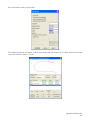
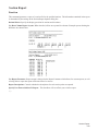
Next we need to make sure that these polylines are closed. In this example, the outside curb polyline is open at
the top. To close the polylines, run Edit->Polyline Utilities->Close Polylines. Then pick each of the pad and curb
polylines and press Enter when done selecting. Here are the Command line prompts:
Select Polylines to set closed.
Select objects: 1 found
Select objects: 1 found, 2 total
Select objects: 1 found, 3 total
Select objects: 1 found, 4 total
Select objects: 1 found, 5 total
Chapter 1. Tutorial
8
Select objects: 1 found, 6 total
Select objects: (Press Enter)
5 polylines already closed.
Closed 1 polylines.
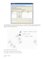
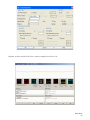
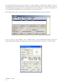
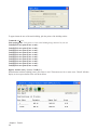
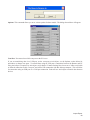
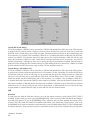
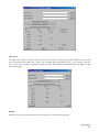
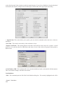
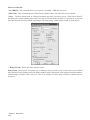
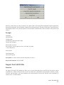
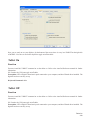
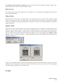
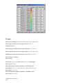
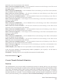
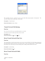
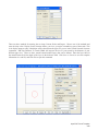
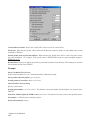
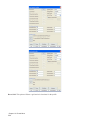
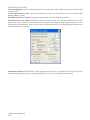
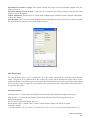
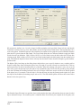
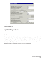
Now run Define Layer Target/Material/Subgrade and pick the Design tab. Highlight layer PAD and pick the Edit
button. A dialog appears for defining the pad material properties. Check on the Include In Material Report option,
enter the Material Name as ''Pad'', set the first subgrade name to ''Pad'', and set the Depth as 1. Once the dialog is
filled out as shown, pick OK.
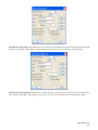
Next pick layer PR-FC-CURB and choose Edit. In the Edit Materials dialog, check on Include In Material Report,
set the Material Name to ''Pavement'', set the first subgrade name to ''Pavement'', and set the Depth to 1.5. Then pick
OK.
To save the subgrade changes, pick the Save button on the Define Layer Targets dialog. Then choose Exit.
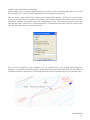
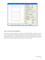
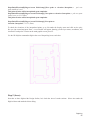
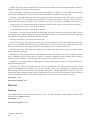
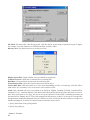
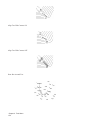
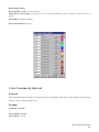
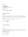
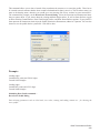
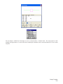
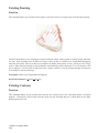
Now let's visually verify the subgrade areas. In the Inquiry menu, run Subgrade Areas->Hatch Subgrade Areas.
There is a dialog to select which subgrade to hatch. Choose the Pavement. Then there is a dialog for the hatch
pattern and color. Click OK. Then run Hatch Subgrade Areas again. This time choose Pad and set the hatch pattern
to Hex with green color. The resulting hatch areas show where the subgrade is applied. Notice how the islands are
not hatched because they are curb polylines that are already inside another curb polyline. Also note that the smaller
pad area is not hatched because this polyline layer is different than the bigger pad polyline. When finished viewing
the subgrade areas, run Inquiry->Subgrade Areas->Erase Subgrade Hatches.
CAD File TakeOff
9
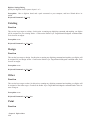
Step 6 (Elevate Drawing - 2D to 3D):
TakeOff will model the existing ground and design surfaces based on points, lines and polylines with elevation. It
is essential for these drawing entities to have correct elevations in order to get correct surface models. Often the
provided drawings will have the drawing entities at elevation of zero with text labels indicating the true elevation.
TakeOff has many tools for assigning elevations to these entities.
To help visualize which entities need to be assigned elevation, TakeOff will color entities at zero elevation in grey.
As entities get assigned elevation, they return to their original color. This elevation coloring is applied to layers that
have been assigned to the existing or design surfaces.
Let's start by working on the existing surface. To isolate the existing entities, go to the Display menu and check on
Existing Drawing, uncheck Design Drawing and uncheck Other Drawing. In the Inquiry menu, there are commands
for checking elevations. To check the elevation of the contour polylines, run the Inquiry->List Elevation and pick a
contour polyline At the command line, it reports the elevation.
Select Entity: pick pad polyline
Elevation: 816.0000
Select Entity (Enter to end): press Enter
In this example, the existing ground surface is defined by just contour polylines and these polylines already have
elevation. So there are no changes needed for preparing the existing surface entities. If the contour polylines were
at zero elevation, then you could use the Elevate->Assign Contour Elevation commands.
Next let's prepare the design surface. To isolate the design entities, go to the Display menu and check on Design
Drawing, uncheck Existing Drawing and uncheck Other Drawing. Notice that all the design linework is greyed
because it is at zero elevation. Run the List Elevation command and pick the main pad polyline. At the command
line, it confirms that the elevation is 0.
To set the pad polyline elevation, run Elevate->Set Polyline To Elevation. Enter an elevation of 818.7 (based on the
text label). At the Select objects prompt, pick the bigger pad polyline and press Enter.
New Elevation <0.0000>: 818.7
Select Lines, Arcs, Circles or Polylines for elevation change.
Select objects: (pick the pad polyline) 1 found
Select objects: press Enter
LWPOLYLINE
Chapter 1. Tutorial
10
Number of entities changed> 1
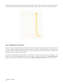
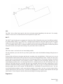
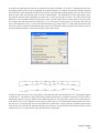
Next let's set the elevation of the smaller pad under the main pad. First, use View->Zoom->Window to zoom in
around the smaller pad so that we can read the text label. The label of ''17.56'' is short for 817.56. In this example,
the 800 was dropped from many of the elevation labels to save on label clutter. Run Set Polyline To Elevation again.
This time enter an elevation of 817.56 and pick the smaller pad polyline. Then run View->Zoom->Previous to get
back to the full view of the site.
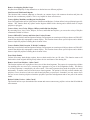
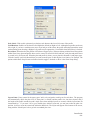
Finally, we need to set the elevations for the curb polylines. First, use View->Zoom->Window to zoom in around
some of the curb labels below the smaller pad. Then run Elevate->2D to 3D Polyline->Text With Leader. This
command will assign the elevations from the labels to the polylines by following the label leader to find the position
on the polyline. For polyline vertices without elevation labels, the elevations will be interpolated from the other
labels. Before processing, this routine prompts for samples of the elevation label, the leader and the polylines to
convert. Then you can select all the entities in the drawing and the routine will sort the labels, leaders and polyline
by the sample layers and assign the elevations. For this example, pick one of the labels with a ''TC'' suffix as the
elevation text sample. Then pick the leader line for the annotation leader sample. Then pick the curb polyline for the
polyline to convert sample. At the Select objects prompt for processing, type ''all'' to select all the drawing entities
and press Enter. For the elevation to add, enter 800 so that labels like ''17.81'' get assigned as 817.81.
CAD File TakeOff
11
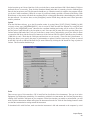
Next a dialog appears for selecting which labels names to use. When TakeOff detects different text labels within
the elevation labels, you need to choose which ones to process. In this case, we only want the labels with ''TC''. So
highlight TC, pick Add and then pick OK.
Select sample of elevation text: pick label
Select sample of an annotation leader: pick leader line
Select sample of a polyline to convert: pick curb polyline
Chapter 1. Tutorial
12
Select polylines to convert, leaders and elevation labels to process.
Select objects: all
Select objects: press Enter
Joining adjacent polylines...
Reading the selection set ...
Enter elevation to add to label values <0.00>: 800
Pre-processing entity #420 of 420
Processing leader #141
Remaking polyline #4
All the curb polylines now have elevations.
Now run View->Zoom->Previous to return to the full site view. The design polylines should now have colors
because the elevations are assigned.
Step 7 (Boundary Polyline):
The limits of the site are defined by a closed polyline. This polyline is used as the boundary for the models and
the volumes. In this example, there is a closed polyline on the PERIMETER layer. The layer target for this layer
is Other. Go to the Display menu and check on Other Drawing so that the perimeter is displayed. Then run Tools>Boundary Polyline->Set Boundary Polyline and pick the perimeter polyline. This selected polyline is now set as
the boundary polyline for the rest of the TakeOff routines.
Step 8 (Model Existing and Design Surfaces):
To calculate volumes, TakeOff needs two surfaces: existing ground and design. These surfaces are modeled by
CAD File TakeOff
13
triangulation. With the preparation of the previous steps, we're now ready to make the models. The drawing entities
have been cleaned up, assigned elevations and assigned target surfaces by layer. Making the models is now a one
step process. To make the existing ground surface, run Tools->Make Existing Ground Surface. The program will
process the entities and make the triangulation surface. Then to make the design surface, run Tools->Make Design
Surface.
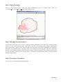
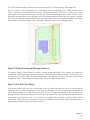
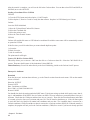
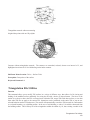
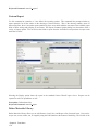
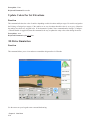
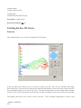
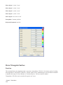
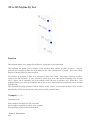
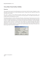
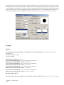
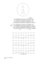
Step 9 (3D Drive Simulation):
As a visual check that the design surface modeled correctly, let's run the View->3D Drive Simulation command.
This routine shows a 3D view of the site and allows you to drive around. This is a good way to check that the
surface modeled correctly. We want to make sure that there are no elevation spikes and that the subgrade depths
are modeled. To drive the site, choose a View Direction, View Position and Vehicle. Then pick the Run button and
use the arrow keys to turn. Pick the Stop button to pause the moving. You can also try the Surface Shading options
for different views of the surface. When done with the 3D Drive Simulation, pick the Exit button (Arrow with door
image).
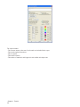
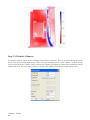
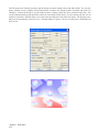
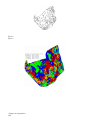
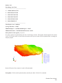
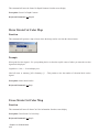
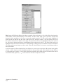
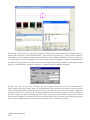
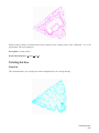
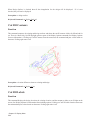
Step 10 (Cut/Fill Color Map):
Cut/Fill color maps can be used for a visual output of the site cut/fill areas and also serves as another check that the
models are correct. In the Display menu, choose Cut/Fill Color Map. Cut areas are drawn in different shades of
red for different depths of cut while fill areas are drawn in blue. To change the resolution of the color blocks, run
Display->Display Options and change the Cut/Fill Color Map Subdivisions. This parameter is the number of rows
and columns of color blocks to create. To turn off the color map, go to the Display menu and pick Cut/Fill Color
Map to uncheck it.
Chapter 1. Tutorial
14
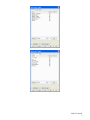
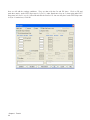
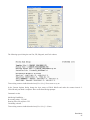
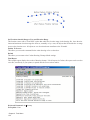
Step 11 (Calculate Volumes):
To calculate volumes, run the Tools->Calculate Total Volumes command. There is an options dialog for setting
the cut swell factor and fill shrink factor. These values get multipled into the cut/fill volumes. Set these factors
as desired and click OK. Then the routine calculates the volumes and display the report which includes the cut/fill
volumes and areas. The report can be printed or saved to a file. Pick the Exit button to exit the report viewer.
CAD File TakeOff
15
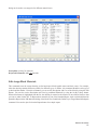
Step 12 (Material Quantities):
To report the quantities, run the Tools->Material Quantities->Standard Report routine. The report includes the
count, length, area and volume for each type of material that was assigned for reporting in the Define Layer Target/Material/Subgrade command. The Material Quantities->Custom Report routine can be used to reporting these
values with control of the report format and the option to export to Excel.
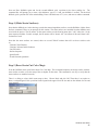
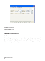
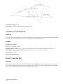
Road Work
This lesson takes a drawing file through the steps of road design.
Step 1 (Start Takeoff):
Click the Windows icon for Takeoff to launch the program. You may be presented with a ''Startup Wizard'' dialog
and if so, click Exit.
Chapter 1. Tutorial
16
Step 2 (Open Drawing):
From the File menu, choose Open and select DEMO2.dwg from the Takeoff Work folder (ie.
C:\Program files\Carlson Takeoff 2004\WORK\DEMO2.dwg).
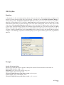
Step 3 (Existing Ground Surface):
For the road cut/fill slopes to be created, it needs the existing ground surface to tie into. First we need to define
the layers of the existing ground surface. Run Tools-> Set Layer For Existing, pick on both a light-lined and
heavy-lined contour, a spot elevation, and press Enter. This will set the layers CTR, CTRINDEX, and TO-PREMSPOT-PNT to the existing surface. The limits of the site are defined by a closed polyline. Run Tools->Boundary
Polyline->Set Boundary Polyline and pick the black polyline around the perimeter. This selected polyline is now
set as the boundary polyline for the existing surface. To make the existing ground surface, run Tools->Make
Existing Ground Surface.
Step 4 (Creating a Centerline):
Now we will use commands under the Roads menu.
Road Work
17
Notice that the Roads menu is broken down into four sections: Centerline commands, Profile commands,
Section commands, and Template commands. A road needs design input from all four sections to be created. It
does not matter in what order the commands are run, but in this example we will run the commands in descending
order.
A centerline file is necessary for the final road design routine. We will do the simplest variation, which is
picking a polyline. There are other methods to design a centerline, and they are documented in the manual. Go
to Polyline to Centerline File in the first grouping of commands under Roads. A file selection dialog will appear.
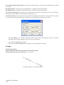
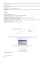
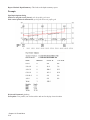
Enter a centerline file name of demo2.cl and pick save. Follow the prompting:
Beginning Station <0+00>: Press Enter
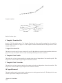
Polyline should have been drawn in direction of increasing stations.
Select polyline that represents centerline: Select the polyline that crosses the middle of the site with the layer name
CLINE.
Station North(y) East(x) Description
———————————————————
0.0000 159718.2034 1857460.9166 LI
1798.2055 159058.6315 1859133.7908 PC
2912.2263 158347.2903 1859964.4134 LI
3755.6840 157619.5351 1860390.7855 LI
Press ENTER to continue.
Your Command Line should have the same values as these, as they are from the same line. Hit the F2 key
or press Enter to return to the main screen.
Step 5 (Input-Edit Profile):
Chapter 1. Tutorial
18
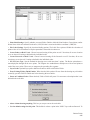
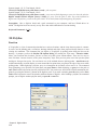
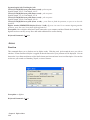
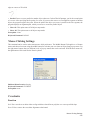
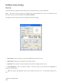
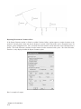
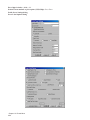
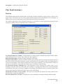
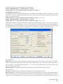
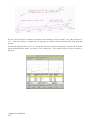
In this routine we will create a Profile file. There are different ways to define a road profile. In this case we will
enter values from a given design. Go to Roads-> Input-Edit Profile File, create a new file, and name it Roaddemo.
The Input-Edit Profile window will be displayed. Under Type of Profile select Road from the dialog box. In the
spreadsheet, you can add design features for the Profile of the road. In this example, enter in the stations 0.0, 1500.0,
and 3755.6840, with elevations of 2030, 2005, and 2040. Next, set the Vertical Curve for the middle station at 300.0.
The Slope Percentages and the Sight Distances are automatically computed for you. Select Save and Exit.
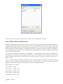
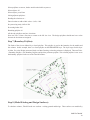
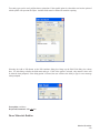
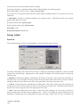
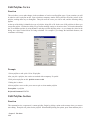
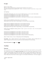
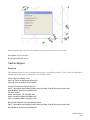
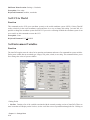
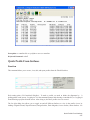
Step 6 (Quick Section):
Now we will create the cross section file (*.SCT). The cross sections define the existing ground for the road to tie
into. Run Roads->Quick Section, fill the dialog as shown, and click OK. Your Offsets should be far enough away
to tie in the Cut/Fill slopes.
Road Work
19
Next, you will be prompted to load a centerline file or to to pick a polyline from the screen. Type C for Centerline
and select the demo2.cl file we created earlier. Your section file is now created, your Command line should read as
follows:
Command: quicksct
Pick starting point (CL-Centerline,P-Polyline): c
Polyline should have been drawn in direction of increasing stations.
Loading edges...
Loaded 4244 points and 12207 edges
Created 7964 triangles
Writing section C:\Takeoff 2004\demo2a-og.sct
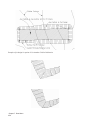
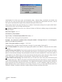
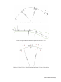
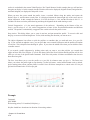
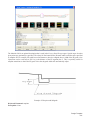
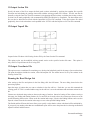
Step 7 (Design Template):
Let's design a wide boulevard with curb and gutter on the outside. The cut slope will be 2:1. In fill, the condition
will be 3:1 in all fill under 6' and 2:1 in all fill over 6' in depth. Pavement depths will be 4'' of asphalt.
First, select Design Template under Roads, name the .TPL file demo2, and open it. A dialog appears where
you enter segments of the template. We will enter a symmetrical template, with 13.5' pavement sections on either
side of the centerline, connecting to a 2' curb and gutter, with 18'' of gutter and 6'' of curb. Then we'll add a 6'
shoulder.
Chapter 1. Tutorial
20
For the lanes, click the Grades Icon.
The above 'child' dialog is shown, enter in: Slope: -2, Horizontal Distance: 13.5, and ID: EP. Click OK.
You'll note that the lanes draw in the little preview window.
Click on the Curb Icon. Fill out as shown below and click OK.
Road Work
21
Next up, we will add a shoulder, going up hill at 4% for 8'. Click on Grades again and enter in a slope of
4, a Horizontal Distance of 8, and the ID as SH.
We are now finished with the surface and can set subgrade. Select the Subgrade icon, second from the right
(yellow color). We will create an asphalt subgrade which will run straight out and hit the curb.
Chapter 1. Tutorial
22
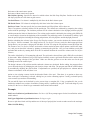
Complete as shown and click OK. Here's what our template looks like so far:
Road Work
23
Now we will add the outslope conditions. They are done with the Cut and Fill icons. Click on Fill and
make three entries: under LEFT Slope enter in 3 (for 3:1), under Depth enter 6 (up to 6'), then again under LEFT
Slope enter in 2 (for 2:1 over 6'). Select OK and click the icon for Cut. Just one entry here: under LEFT Slope enter
in 2 (for 2:1 normal cut). Click OK.
Chapter 1. Tutorial
24
Now click Save. The template is complete.
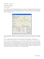
Step 8 (Process Road Design):
This is the routine that weaves everything together. Select Process Road Design, the last command in the Roads
menu. The Specify Input Files column on the left allows you to choose the files to be used in the road design. We
have already created the four needed files, go ahead and select them now and then click OK.
Road Work
25
In the next dialog you can select different output features. For 3D viewing in the next step, toggle on Triangulate & Contour . It can be found in the bottom left portion of the Additional Earth Works Parameters dialog.
Click OK.
Note: To generate a plot of road sections, specify an output section file in the 1st Road Design dialog. Then run
Draw Sections in the Roads menu.
Chapter 1. Tutorial
26
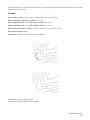
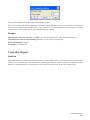
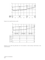
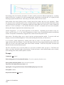
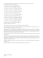
The following report listing the total Cut, Fill, Subgrade, and Curb volumes.
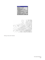
Trim existing contours inside disturbed area [Yes/<No>]? Press enter to say no
In the Contour Options dialog change the layer name to FINAL ROAD and make the contour interval 2.
Click OK and your Road is complete! Here are the Road Design prompts:
Command: eworks
Initializing EarthWorks ...
Processing station: 3755.680
Drawing offset 3D polylines: TIE
Calculating volumes ...
Trim existing contours inside disturbed area [Yes/<No>]? <Enter>
Road Work
27
Reading points... 2631
Inserted 2631 points
Inserted 2618 breakline segments
Drawing Triangulation 3D Faces ...
Contouring elevation 2040
Inserted 811 contour vertices.
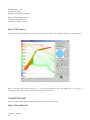
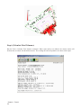
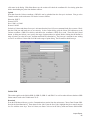
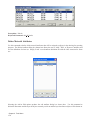
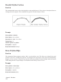
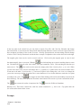
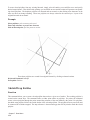
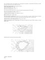
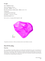
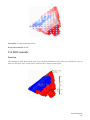
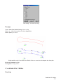
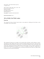
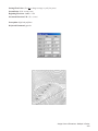
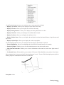
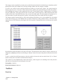
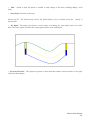
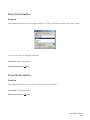
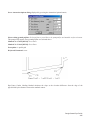
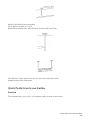
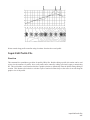
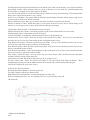
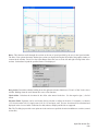
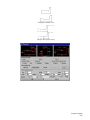
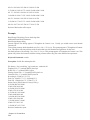
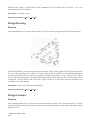
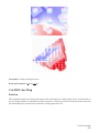
Step 9 (3D Viewer):
Now that your Road is complete lets view it in 3D. Go to View, 3D Viewer Window, type in ALL, and press enter.
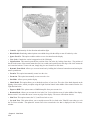
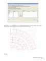
Here is our road with a Vertical Scale of 4. Color By Elevation has also been toggled on. Use the X, Y,
and Z control bars at the bottom to rotate the drawing in the 3D viewer.
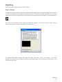
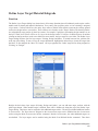
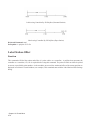
Trench Network
This lesson takes a drawing file through the steps of trench network quantities.
Step 1 (Start Takeoff):
Chapter 1. Tutorial
28
Click the Windows icon for Takeoff to launch the program. You may be presented with a ''Startup Wizard'' dialog
and if so, click Exit.
Step 2 (Open Drawing):
From the File menu, choose Open and select DEMO3.dwg from the Takeoff Work folder (ie.
C:\Program files\Carlson Takeoff 2004\WORK\DEMO3.dwg).
Trench Network
29
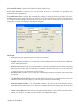
Step 3 (Make Existing and Design Surfaces):
In order to calculate trench quantities and profiles, we need surfaces for the existing ground and design.
First we need to define the layers of the surfaces. Run Tools->Define Layer Target/Material/Subgrade.
Then from the tab labeled ''Other'', highlight ''EX CTR'' from the layer list, pick ''Existing'' from the Move To list
and pick the Move To button. Next, highlight ''RD RF CONT'', choose ''Design'' from the Move To list and pick the
Move To button. Now choose the Save and then Exit buttons. This assigned layer ''EX CTR'' to the existing ground
surface and ''RD RF CONT'' to the design surface.
Next, let's set the site perimeter. Run Tools->Boundary Polyline->Set Boundary Polyline. At the command
line, there is a prompt:
Select boundary polyline:
Pick anywhere along the six sided perimeter polyline in the drawing.
Now, to make the existing ground surface, run Tools->Make Existing Ground Surface.
design surface, run Tools->Make Design Surface.
Then to make the
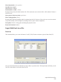
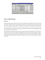
Step 4 (Input Trench Network Data):
The trench network data consists of linked structures where each structure has a name, location (x,y), invert-in,
invert-out and rim elevation. Each structure link has a pipe size. There are two ways of entering the trench data.
When the drawing contains polylines for the trench lines and labels with the trench data, then you can use Input
Trench From Polyline. Otherwise, there is the Create Trench Network Structure command which let's you pick the
structure locations and enter the data in a dialog.
Chapter 1. Tutorial
30
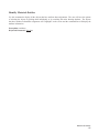
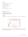
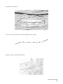
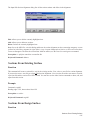
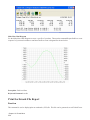
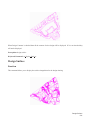
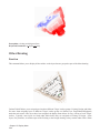
Method 1 (Input Trench Data From Polyline):
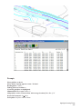
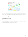
In this example, there is trench data already drawn in the drawing. Zoom in around the upper right area of trench
line by running View->Zoom->Window and picking two corner points around this area.
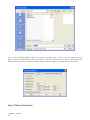
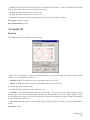
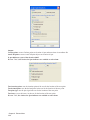
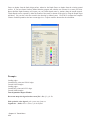
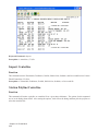
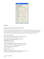
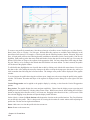
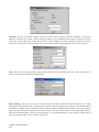
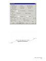
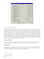
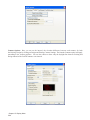
Then run Trench->Input Trench From Polyline and an options dialog appears. In this case, we want Trench
Type as Sewer because there are manhole rim elevations. Also Prompt For Invert-In Elevations is active since this
example has a manhole with multiple connections with different invert-ins. And Connected Network is used so that
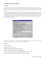
the trench data can be used by the rest of the trench routines. The Individual Profile option will only create a profile
(.pro) file. Fill out the dialog as shown and click OK.
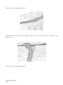
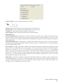
The rest of the prompting for this command is on the command line as the program walks through the
trench line. For each point in the trench polyline, the program zooms the drawing to that point. The trench data can
be picked from labels in the drawing. If the drawing doesn't have labels for the data, then you can enter the values.
Trench Network
31
Pick a polyline that represents a trench reach: Pick the trench polyline
Starting Station of trench reach <0.0>: 0.0
For station 0.00 ...
Enter/<Select text of Manhole ID>: Pick the DCB 368 label. (If you had a drawing without a manhole ID label,
then type E for Enter and enter the ID)
ID: DCB 368
Undo/Enter/<Select text of Invert-in elevation>: Pick the I Out=174 label. (Since this is the upstream starting
manhole, there really isn't a separate invert-in. So we are using the invert-out).
Invert-In: 174.000
Undo/Enter/<Select text of Invert-out elevation>: Pick the I Out=174 label.
Invert-Out: 174.000
Undo/Enter/<Select text of manhole rim elevation>: Pick the R=178.75 label.
Rim: 178.750
For station 201.44 ...
Enter/<Select text of Manhole ID>: Pick the DCB 367 label.
ID: DCB 367
Undo/Enter/<Select text of Invert-in elevation>: Pick the I In=172.85 label.
Invert-In: 172.850
Undo/Enter/<Select text of Invert-out elevation>: Pick the I Out=172.35 label.
Invert-Out: 172.350
Undo/Enter/<Select text of manhole rim elevation>: Pick the R=178.5 label.
Rim: 178.500
Undo/Enter/<Select text of pipe size>: Pick the 15'' HDPE label.
Pipe Size: 15.0
For station 327.09 ...
Enter/<Select text of Manhole ID>: Pick the CB 347 label.
ID: CB 347
Undo/Enter/<Select text of Invert-in elevation>: Pick the I In=170.540 (CB 367) label. (This is the invert-in for
the connection to the CB 367 structure that this trench line connects to.)
Invert-In: 170.540
Undo/Enter/<Select text of Invert-out elevation>: Pick the I Out=166.1 label.
Invert-Out: 166.100
Undo/Enter/<Select text of manhole rim elevation>: Pick the R=176.5 label.
Rim: 176.500
Undo/Enter/<Select text of pipe size>: Pick the 15'' HDPE label.
Pipe Size: 15.0
Another Polyline [<Yes>/No]? N for no.
That completes this trench run and Takeoff draws its own trench polyline and labels.
Method 2 (Create Trench Network Structure):
The drawing contains another trench polyline and we could use Input Trench Data From Polyline again. Instead for
practice, let's use the Create Trench Network Structure method. First we need to zoom to the new trench location.
Run View->Zoom->Extents and then View->Zoom->Window and pick two points for a window around the lower
right trench point (CB 349). Then run Trench->Create Trench Network Structure. At the command line, there is a
prompt for how to locate the structure position. Choose Pick.
Locate by pick point, point number or station-offset [<Pick>/Number/CL]? Pick
Chapter 1. Tutorial
32
Next, there is a prompt to pick the position. To get the exact end point of the trench polyline, use the end point snap.
The end point snap can be turned on by a number of different ways including the Settings->Object Snap command.
In this case, type ''end'' and then space or enter. This puts the program in end point snap mode. Now move the
pointer along the trench polyline until the end point snap icon is at the manhole location and then pick.
Pick structure location: end of (pick point)
Now a dialog appears for entering the structure data. Fill in the Structure Name as CB 349, the Rim Elevation as 187.8 and the Invert-Out as 178.3 and then pick OK.
All the structures are now created. The last step is to link this new structure to the network. We need to zoom to
the next trench location. Run View->Zoom->Extents and then View->Zoom->Window and pick two points for a
window around the left trench point (CB 347). Now run Trench->Edit Trench Network Structure and pick either the
symbol for CB 347 or the label. Then a dialog appears with the data for CB 347. From the Available list, highlight
CB 349 and pick Add. This creates a link from CB 347 to CB 349 and the link data is shown at the bottom of the
Trench Network
33
dialog. Enter the Invert-In as 171 and the Pipe Size as 24. Then pick OK.
Step 5 (Input-Edit Trench Template):
The Trench Template defines the size of the trench for quantities. Run Trench->Input-Edit Trench Template. You
are first prompted for a trench template file name. The Trench Template data is stored in a file that has a .tch
extension. Choose the New tab, enter a file name like DEMO3 and then pick Open.
Next, there is a dialog for entering the trench dimensions. The Bottom Offset is the distance from the bottom of the pipe to the bottom of the trench. The Trench Width is the base width of the trench. The Vertical Side
Height is the height from the bottom that the side walls are vertical until switching to the cut slope. If the surface
is not reached by the vertical side height, then the cut slope is used for the rest of the distance to the surface. Edit
Trench Benches allows you to set up to four benches in your trench. Display Sewer Structure allows you to see your
pipe or manhole as part of the trench. Note: This is for display purposes only, calculations will be drawn from the
pipe size you set in the Trench Network Structure commands. Add Pipe Diameter To Trench Width will increase
the size of your trench by the diameter of your different pipe sizes. The Cut Slope can be entered in slope percent,
ratio or degree format. The Backfill materials are optional. Up to three materials can be entered from the bottom.
Fill out the dialog as shown and pick Save and Exit.
Chapter 1. Tutorial
34
Step 6 (Trench Network Quantities):
To calculate and report the trench quantities, run Trench->Trench Network Quantities. A dialog sets the report
options. Check on Calculate All Trenches to get the quantities for the whole network. To get the trench cut volume,
check Use Trench Template For Quantities and pick Set Trench Template and pick DEMO3.TCH. Also turn on
Report Backfill Volumes to use our backfill material settings from the trench template. Finally, fill out the depth
zones in the intervals that you are interested in. In this case, use 15, 20 and 25. The depth zones will be colored in
the plain view. Once the dialog is filled out as shown, pick OK and the report is shown.
Trench Network
35
The report includes:
- The structure names at the start of each trench run included in the report.
- The trench template dimensions.
- The cut volume.
- The backfill volumes.
- The number of manholes and length of trench within each depth zone.
Chapter 1. Tutorial
36
The depth zones in the plain view with Zone Map Color Legend.
Step 8 (Draw Trench Network Profile):
Trench Network
37
To draw a profile of the trench line, run the Trench->Draw Trench Network (Profile) command. There is a dialog to
select the starting structure for which trench line to process. Choose DCB 368. Also, there are options whether to
draw the existing ground, design surface and strata surfaces if available. You can also choose the profile direction
to go upstream or downstream. The Save To Profile File will create a profile (.pro) file for the trench. Fill out the
dialog as shown and pick OK.
Next the Draw Profile dialog appears. Set the Horizontal Scale and intervals to 50 and the Vertical Scale
and intervals to 25. This will make for two to one vertical exaggeration for the profile. When the dialog is filled out
as shown, pick OK.
Chapter 1. Tutorial
38
Next, there are prompts at the command line for the profile grid elevations and profile location.
Bottom Elevation of Profile Grid <150.0>: Press Enter
Top Elevation of Profile Grid <200.0>: Press Enter
Pick Starting Point for Grid <409458.0 , 207303.0>: Pick a point in a blank area off to the side of the drawing.
Next there are two dialogs with lots of settings for how to draw and label the trench profile. Let's go with
the defaults except change the Type Of Pipe to HDPE. When the settings are ready, click the OK button for each
dialog.
Trench Network
39
There is a final command line prompt for whether to use the manhole elevations. Enter Yes which will use
the rim elevations defined in our trench network.
Use manhole elevations from profile [<Yes>/No]? Y for yes.
The profile shows the existing ground at the top, then the design surface and then the trench.
Chapter 1. Tutorial
40
Drillhole and Strata
This lesson creates and processes drillhole data.
Step 1 (Run Lesson 1 Example):
This drillhole lesson builds on the resulting drawing called demo1.dwg from the tutorial lesson 1 (CAD File
Takeoff). Before continuing with this tutorial, run through and complete this lesson 1 tutorial.
When lesson 1 is done, let's set the display to show only the design entities. In the Display menu, turn off
Existing Drawing and Other Drawing and turn on Design Drawing. Then run, View->Zoom->Extents. Now we're
ready to add drillholes.
Step 2 (Drillhole/Strata Settings):
From the File menu, choose Drillhole/Strata Settings. This command sets the drillhole symbol and the default strata
names. For this tutorial, we are interested in rock quantities and we need to define two strata: Dirt (material above
the rock) and Rock.
Drillhole and Strata
41
Pick the Add button which brings up another dialog that defines a strata. Enter a strata name of ''DIRT'' and a density
of 125 which will be used to calculate tons in the volume report. You can also have a strata specific cut swell factor.
The strata can be modeled either by the elevations from the drillholes or by the depth from the existing ground. In
this case, we will model by strata elevation. When the dialog is filled out as shown, pick OK.
Next, pick the Add button again. This time, fill out the dialog with a strata name of ''ROCK'' and density of 150.
Then pick OK.
The Strata Definitions in the main dialog need to be in top to bottom order. To change the order, highlight a strata
name and use the Move Up or Move Down buttons. In this case, we want Dirt then Rock. Click OK now from the
main dialog.
Step 3 (Input Drillhole Data):
There are two different methods for entering drillhole data into Takeoff: Drillhole Import and Place Drillhole.
Drillhole Import reads the drillhole data from a text file. This command supports customizing the sequence of
drillhole data fields to match the format of the text file. Place Drillhole creates the drillholes at picked positions in
the drawing and enters the data in a dialog. For this tutorial, we will use Place Drillhole.
Chapter 1. Tutorial
42
Run the Drillhole->Place Drillhole command. At the command line, there is a prompt to pick the drillhole
location. If you know the coordinates for the drillhole, you can type in the easting,northing instead of picking on
the screen. In this case, let's pick a point above the upper right of the main building.
Pick Drillhole Location: pick a point
Then there is a dialog for entering the drillhole data. The surface elevation is automatically filled in using
the existing ground surface model. The Drillhole Name and Description are optional. The list of strata defaults to
the strata defined in Drillhole/Strata Settings. Each strata defaults to a thickness of zero. To set the strata thickness,
highlight the strata and pick the Edit button.
For this case, highlight Dirt and pick Edit. This brings up the Edit Strata dialog. The strata position can be
defined by thickness, elevation or depth. Setting any one of these fields will update the other fields. For our dirt
stata, fill in a thickness of 2 and then pick OK.
Drillhole and Strata
43
Next, pick Rock from the strata list and pick Edit. For this example, we only know the depth to the top of
rock depth and not the total rock thickness. We will treat all cut below the top of rock as rock strata. So we will set
the rock thickness deep enough to be lower than the deepest cut on site. In this case, we will use a rock thickness of
15. So in the Edit Strata dialog for rock, enter a thickness of 15 and then pick OK.
After editing the rock strata, we are returned to the main Edit Drillhole dialog. Pick the Save button.
Now let's locate two more drillholes using a different method. Return Drillhole/Strata Settings dialog and
change Place Drillhole Prompts to Thickness. Also, check on Default Thickness and set it to 15 feet, Press OK.
Chapter 1. Tutorial
44
Now run Place Drillhole again and for the second drillhole, pick a position in the lower parking lot. The
command line will prompt you to enter a dirt thickness, type in 1.5 and your drillhole is created. For the third
drillhole, pick a position left of the main building. Enter a dirt thickness of 3.0, save, and enter to end the command.
Step 4 (Make Strata Surfaces):
Now that the drillholes are in the drawing, to make the strata triangulation surfaces, run the Drillhole->Make Strata
Surfaces command. There are no prompts for this routine. The strata surfaces are modeled from the drillholes and
saved with the project. The file names for the strata surfaces use the drawing name plus ''-ch#'' where the # is the
strata sequence number. For this example, the file names will be ''demo1-ch1'' for bottom of dirt and ''demo1-ch2''
for bottom of rock.
Now that the strata surfaces are created, there are several Takeoff routines that will use these surfaces such
as:
- Calculate Total Volumes
- Calculate Volumes Inside Perimeter
- Cut/Fill Labels
- Surface Inspector
- Quick Profile
- Trench Network Quantities
Step 5 (Draw Strata Cut Color Map):
From the Drillhole menu, pick Draw Strata Cut Color Map. This command compares the design surface with the
strata surface to make a cut color map of the cut depths for the strata. This command is one way to verify that the
strata surfaces are modeled correctly.
There is a dialog to select which strata map to draw. Choose Rock and pick OK. Then there is an option to
draw a cut depth legend. Pick a position for the legend in the upper left of the site and use the defaults for size and
zone summary.
Drillhole and Strata
45
Step 6 (Calculate Total Volumes):
Run the Tools->Calculate Total Volumes command. When strata surfaces are defined, the volume routine will
breakout the cut volume into the different strata. The resulting dirt and rock quantities are shown in the report.
Chapter 1. Tutorial
46
Digitizing
This lesson tranfers a paper plan into Carlson Takeoff.
Step 1 (Setup):
To digitize in Carlson Takeoff, you need to install the Wintab digitizer driver. See Digitizer Setup in the manual if
you have not installed or have problems with the Wintab driver. If Wintab is installed, then make sure your drawing board is on and take the paper plan provided with the Carlson Takeoff manual and place it on your drawing board.
Now, click on the Windows icon for Takeoff to launch the program. You may be presented with a ''Startup
Wizard'' dialog similar to the one shown below, if so click New.
If a Startup Wizard did not appear, then under File menu, select New to start a new drawing. You will be
prompted for a template to use. Templates determine the default settings for your drawing. For this tutorial, select
site.dwt and click Open.
Digitizing
47
Next, the New Drawing Wizard appears for setting the drawing name. Click on the Set button at the top
dialog. In the file selection dialog, enter the file name of ''digitize'' and pick the Save button. Then Exit the New
Drawing Wizard. From here, a Data Files dialog appears where no changes are needed. Pick the Exit button.
Step 2 (Tablet Calibration):
Chapter 1. Tutorial
48
To start things off, you need to set the coordinate system for the paper plan by running the Calibrate command
under Digitize menu and sub-menu Tablet. Calibration is required to let the program know the orientation and scale
of the paper plan.
There are two different Calibration Methods: Known Reference Points and Drawing Scale with New Reference Points. Known Reference Points allows you to enter in the coordinates of two marked points on the paper plan.
This method applies when you know the coordinates of at least two points on the paper plans. Drawing Scale with
New Reference Points allows you to setup a coordinate system for the plans by entering the plan scale and picking
any two points from the paper plan with the digitizer puck.
In this case, we will use Drawing Scale with New Reference Points. First, enter in the Drawing Scale listed
on the paper plan. On this drawing, the scale is 1:40, so enter in 40. Use the default coordinates for Point 1 and
click OK. Now Carlson Takeoff will prompt you for your First and Second Reference points. Generally, you want
to pick to points on the drawing that you can find and use again in case you need to recalibrate. Also, the further
away the points are from each other, the more accurate the coordinate system will be. With the digitizer puck,
icon in the lower left and upper right of the drawing for the two Reference Points. The firstpoint is
pick on the
assigned the coordinates of 1000,1000 from the dialog and the second point is assigned coordinates to match with
the plan scale. From now on, all of your points will be in relation to these two points.
Digitizing
49
Step 3 (Digitizing Existing Contours):
We will now digitize the existing contours. Under the Digitize menu, click on Existing and then go to Contour
Polyline, and this dialog will appear. Enter in a Layer Name of XCONT and select OK. Note: your Elevation
Interval should match the intervals marked on your paper drawing. In this drawing, the interval is the same as the
default of 1.00.
The rest of the prompting occurs at the command line and starts with the contour elevation. Find the lowest
elevation for the existing contours labeled in bottom right corner of the paper plan zoomed in on below. In this
example, the lowest elevation is 624 feet. The elevation can be entered either with the digitizer puck keys or with
the computer keyboard. The layout of the digitizer keys is set in Digitizing Settings->Puck Layout. Press Enter
Chapter 1. Tutorial
50
after you have entered in 624. You want to enter in the lowest contour so that as Carlson Takeoff adds the Elevation
Interval, it is from lowest to highest.
Next, you will see the following prompt:
Sketch[0]/Exit[A]/Pick the first point:
There are two different ways to digitize: in Pick Mode or Sketch Mode. You can switch between them at anytime.
In this tutorial we will run through how to do both. For now, type in [0] and press enter to get into Sketch Mode. In
Sketch Mode, you will be prompted to Pick and drag. The point you pick is the starting point of a contour. Drag
is asking you to follow that contour with the digitizer puck on the paper plan. Click a second time when you have
traced the entire contour and have reached the end of the contour. You will then be prompted as follows:
Pick[0]/Close[A]/Undo[B]/Pick and drag (Enter to end):
Type in [B] for Undo if you made a mistake and need to sketch part of the contour again. [A] will close the
contour, and [0] will switch you into Pick Mode. We still have more existing contours to digitize, so press Enter
to end and answer yes to the Digitize Another Contour prompt. Takeoff will prompt you to verify the elevation.
Remember, we set the Elevation Interval to one, so the default elevation for your next contour line is 625, press
Enter. Now, pick the endpoint of the next contour and trace it in the same manner as the previous contour.
Now let's try Pick Mode. Say yes to digitize another contour and check to see if the default elevation corresponds with the contour your about to digitize. If not, simply type in the correct number in the command line. Next,
pick [0] to get into Pick Mode. In Pick Mode, you do not have to trace the contour. Rather, pick with the digitizer
puck to create points that will make up the contour. Note: Less picks are needed on fairly straight segments.
Digitizing
51
Conversely, more picks will give you a more acurrate contour. Press Enter when you have reach the end of the
contour. Repeat this until you have digitized all of the existing contours you want to have in Takeoff (see below).
Step 4 (Digitizing the Design):
Now we will digitize the building and curb linework of the Design Surface using the Digitize 2D Polyline and 3D
Polyline commands. Besides drawing the linework positions, we will also assign layer names to the linework that
we will use later to identify the types of linework. In this example, there are no design contours, only the design
building and curb linework and spot elevations.
Let's begin by digitizing the main building. Under Digitize, check on Design and go to 2D Polyline. 2D
Polyline is used to digitize linework enities with one elevation. Toggle off the check box Use current drawing
layer and name the layer NEW BUILD. Toggle on the Prompt For Polylne Elevation option. Then click OK.
Chapter 1. Tutorial
52
At the command line, enter in the building elevation of 634.41 found labeled in the middle of the building
and press Enter. Then pick the points that define the building outline. Start in the upper left corner and pick at
every corner around the building. When you have picked around the entire building, type in [A] for close to finish
digitizing the building.
Enter polyline elevation <0.00>: 634.41
First point: pick a building point
Close[A]/Undo[B]/Osnap[.]/Pick next point (Enter to end): pick the next building point
Close[A]/Undo[B]/Osnap[.]/Pick next point (Enter to end): pick the next building point
Close[A]/Undo[B]/Osnap[.]/Pick next point (Enter to end): pick the last building point
Close[A]/Undo[B]/Osnap[.]/Pick next point (Enter to end): A to close
Digitize Another NEW BUILD Polyline [Yes(A)/<No(B)>]? B for No
Notice that the parking lot linework consists of different elevation levels. To digitize entities with more than
one elevation, go to Digitize and select 3D Polyline from the pull-down menu. Make sure that the Prompt For
Polyline Elevation option is on, the Use current drawing layer toggle is off and name the layer NEW EDGE
ASPH.
Digitizing
53
Let's start by digitizing the parking lot starting from the zoomed in section below. The edge of asphalt is
the inside line. The parking lot elevation labels have been shortened on the paper plan. For example, they read
35.37 and 35.12, when the actual elevations are 635.37 and 635.12. Enter in 600 as the Elevation Adder, then click
OK.
Click on the point with the digitizer puck where the 35.37 elevation label points to in the upper left corner
of the parking lot. When prompted for Elevation enter in 35.37. Pick below the first point where the linework starts
to curve. We do not have an elevation for this point, but we can interpolate the elevation from the two points around
it using the interpolate option. Type in I for interpolate or hit the A button on the Puck. Next pick the middle point
of the curve and again use Interpolate for the elevation. Next pick the end of the curve at the 35.12 label and enter
in the elevation 35.12. Continue digitizing for the rest of the edge of asphalt linework. Digitize each point where
there is an elevation label and each point where the curb line changes direction.
The first prompts should resemble these:
First point: pick first point (at 35.37 label)
Interpolate[A]/screen Pick/<Elevation[B]> <0.00>: 35.37
Z: 635.37
Close[A]/Undo[B]/Osnap[.]/Pick next point (Enter to end): pick next point (start of curve)
Slope/Ratio/Interpolate[A]/Degree/screen Pick/<Elevation[B]> <635.37>: Press the [A] button on the Puck
for Interpolate
Chapter 1. Tutorial
54
Slope/Ratio/Elevation[B]/Degree/screen Pick/Osnap[.]/Next point or elevation<Interpolate>: pick next
point (middle of curve)
This point elevation will be interpolated upon completion.
Slope/Ratio/Elevation[B]/Degree/screen Pick/Osnap[.]/Next point or elevation<Interpolate>: pick next point
(end of curve, at 35.12 label)
This point elevation will be interpolated upon completion.
Slope/Ratio/Elevation[B]/Degree/screen Pick/Osnap[.]/Next point or
elevation<Interpolate>: 35.12 (Enter)
To check the elevations of the interpolated points go to List under the Inquiry menu and click on the polyline you just created and press Enter. A text window will appear showing you the layer name, coordinates, and
elevation of each point. To return to the main graphic screen, press F2.
Use the 3D Polyline command to digitize the rest of the parking lot as seen below.
Step 5 (Area):
Now that we have digitized the Design Surface, let's check the Area of certain sections. Select Area under the
Digitize Menu and match the below dialog.
Digitizing
55
To approximate the area of the main building, pick the points of the building outline.
Command: dig area
Pick starting point: Pick points as close to the building design linework as you can
Undo[B]/Pick next point (Enter to end):
Undo[B]/Pick next point (Enter to end):
Undo[B]/Pick next point (Enter to end):
Undo[B]/Pick next point (Enter to end):
Undo[B]/Pick next point (Enter to end):
Undo[B]/Pick next point (Enter to end):
Undo[B]/Pick next point (Enter to end):
Undo[B]/Pick next point (Enter to end):
Undo[B]/Pick next point (Enter to end):
Undo[B]/Pick next point (Enter to end):
Digitize Another Area [<Yes(A)>/No(B)]? B
When finished with the building points, press Enter to end. Then answer no for no more areas. Takeoff will then
display an Area report similar to the one shown below.
Chapter 1. Tutorial
56
Step 6 (Spot Elevations):
In our paper drawing, we have two spot elevations labeled 32.57 and 32.41 shown in the bottom left below.
To digitize these elevations, we can use the Spot Elevation command under the Digitize menu. Fill out the
Spot Elevation dialog as shown and pick OK.
Digitizing
57
In the paper plan, find and click on the spot elevations with the puck. When prompted, enter in their corresponding elevations of 632.57 and 632.41.
Step 7 (Boundary Polyline):
The limits of the site are defined by a closed polyline. This polyline is used as the boundary for the models and the
volumes. Under the digitize menu, check on Other and then select Perimeter. Type in PERIMETER as the layer
name. Now digitize around the bold, outside line shown below.
Say No to the prompt: Digitize Another PERIMETER Polyline [Yes(A)/<No(B)>]?
Now run Tools->Boundary Polyline->Set Boundary Polyline and pick the perimeter polyline. This selected
polyline is now set as the boundary polyline for the rest of the Takeoff routines.
Step 8 (Layer Targets):
From the Tools menu, choose Define Layer Target/Material/Subgrade. Every entity (line, polyline, point, etc) in the
drawing is assigned a layer name. Takeoff uses the entity layer names to define which entities are for the existing
ground surface, the design surface or no surface. These surfaces are referred to as the ''Target'' surfaces. The drawing
entities are assigned their target surface by their layer name. For example, if polylines representing design contours
Chapter 1. Tutorial
58
are on the layer ''NEW'', then ''NEW'' will be set as a layer for the design surface. For layers of entities that are for
neither existing nor design surfaces (such as text labels for street names), the layer target is set to Other.
The Define Layer Targets dialog has three lists of layers: Existing, Design and Other. To switch between lists, pick
the tabs at the top of the dialog. We have already defined the layers for their correct targets. We did this by check
on Existing, Design, or Other in the pull-down menu.
Check that your Layer Targets resemble the three lists shown here. If a layer is out of place, highlight it, and hit the
''Move To'' button after selecting the correct target to send it to. After reviewing, pick Save and Exit.
Digitizing
59
Now that the layer targets are defined, there are several commands that can be applied. In the Display menu, you can
turn on/off whether to display layer targets by using Existing Drawing, Design Drawing and Other Drawing, or by
right-clicking with your mouse. For example, when Design Drawing is checked, then picking this menu item will
uncheck it and turn off all the layers for the design surface. Likewise, picking Design Drawing when it is unchecked
will make it checked and turn on the design surface layers.
Practice turning on/off the Existing, Design and Other Drawing in the Display menu. When only Existing Drawing
is on, you should see just the contours. When only Design Drawing is on, you should see just the design polylines
Chapter 1. Tutorial
60
and leader labels. When only Other Drawing is on, you should see the entities that are assigned to neither existing
nor design.
Step 9 (Define Material/SubGrade):
Besides assigning target surfaces by layer, layers are also used to define material names and subgrade depths. By
assigning material names and depths to layers, the volume, area, length and count for entities on these layers can be
reported. Also the depth is used to vertically adjust the design surface. The polylines used for subgrade depth must
be closed polylines. Takeoff supports nested subgrade polylines for exclusion areas such as islands by counting how
many subgrade polylines surround an area. If the number is odd, then the area is inside the subgrade. Otherwise the
area is not part of the subgrade.
First, let's confirm the layer names for our subgrades. Go to the Display menu and check on Design Drawing,
uncheck Existing Drawing and uncheck Other Drawing. Then run Inquiry->Layer ID and pick the large pad polyline. It reports that this layer is NEW BUILD. Next use Layer ID to pick the curb polyline. It reports that this layer
is NEW EDGE ASPH.
Now run Define Layer Target/Material/Subgrade and pick the Design tab. Highlight layer NEW BUILD and pick
the Edit button. A dialog appears for defining the pad material properties. Check on the Include In Material Report
option, enter the Material Name as ''Pad'', set the first subgrade name to ''Pad'', and set the Depth as 1. Once the
dialog is filled out as shown, pick OK.
Digitizing
61
Next pick layer NEW EDGE ASPH and choose Edit. In the Edit Materials dialog, check on Include In Material
Report, set the Material Name to ''Pavement'', set the first subgrade name to ''Pavement'', and set the Depth to 1.5.
Then pick OK.
Chapter 1. Tutorial
62
To save the subgrade changes, pick the Save button on the Define Layer Targets dialog. Then choose Exit.
Now let's visually verify the subgrade areas. In the Inquiry menu, run Subgrade Areas->Hatch Subgrade Areas.
There is a dialog to select which subgrade to hatch. Choose the Pavement. Then there is a dialog for the hatch
pattern and color. Change the color to green and click OK. Then run Hatch Subgrade Areas again. This time choose
Pad and set the hatch pattern to Hex with blue color. The resulting hatch areas show where the subgrade is applied.
Notice how the islands are not hatched because they are curb polylines that are already inside another curb polyline.
When finished viewing the subgrade areas, run Inquiry->Subgrade Areas->Erase Subgrade Hatches.
Step 10 (Model Existing and Design Surfaces):
To calculate volumes, Takeoff needs two surfaces: existing ground and design. These surfaces are modeled by
triangulation. With the preparation of the previous steps, we're now ready to make the models. To make the existing
ground surface, run Tools->Make Existing Ground Surface. The program will process the entities and make the
triangulation surface. Then to make the design surface, run Tools->Make Design Surface.
Step 11 (Cut/Fill Color Map):
Cut/Fill color maps can be used for a visual output of the site cut/fill areas and also serves as a check that the
models are correct. In the Display menu, choose Cut/Fill Color Map. Cut areas are drawn in different shades of
red for different depths of cut while fill areas are drawn in blue. To change the resolution of the color blocks, run
Display->Display Options and change the Cut/Fill Color Map Subdivisions. This parameter is the number of rows
and columns of color blocks to create. You can also draw a legend for the Color Map by going to Draw, Cut/Fill
Map Legend. Pick a point on your drawing to locate the legend and press Enter. To turn off the color map, go to the
Display menu and pick Cut/Fill Color Map to uncheck it.
Digitizing
63
Step 12 (Calculate Volumes):
To calculate volumes, run the Tools->Calculate Total Volumes command. There is an options dialog for setting
the cut swell factor and fill shrink factor. These values get multipled into the cut/fill volumes. Set these factors
as desired and click OK. Then the routine calculates the volumes and display the report which includes the cut/fill
volumes and areas. The report can be printed or saved to a file. Pick the Exit button to exit the report viewer.
Chapter 1. Tutorial
64
Step 13 (Material Quantities):
To report the material quantities, run the Tools->Material Quantities->Standard Report routine. The report includes
the count, length, area and volume for each type of material that was assigned for reporting in the Define Layer
Target/Material/Subgrade command. The Material Quantities->Custom Report routine can be used to reporting
these values with control of the report format and the option to export to Excel.
Digitizing
65
Chapter 1. Tutorial
66
AutoCAD Overview
2
67
Issuing Commands
Carlson Takeoff is build on the AutoCAD engine. This section will review some basics of AutoCAD that will be
useful in running Carlson Takeoff.
Virtually all commands in AutoCAD have three or more ways they can be initiated. The two most common are the
menu (if you can find the command you want) and the toolbar (those cute little buttons), but the command line (DOS
lives!) can many times be a very easy method of working through commands. Using the menu and toolbar should
be second nature to Windows users, so this section will mainly focus on the command line usage in AutoCAD.
Command Line Prompt-Command:
AutoCAD has a command line prompt where commands are ''issued'' and the status of a command is reported.
When you select a command from the menu or toolbar, that command name is sent to the command line and is
executed. Before most commands can begin, all other commands must be terminated. The exceptions are referred
to as transparent commands. The easiest way to see if no commands are running is to look at the command line. If
it displays Command: no commands are currently in progress.
Enter
When you are required to press the Enter key in AutoCAD, you can use the Enter key on the keyboard or you can
press the spacebar or click the right mouse button.
Pressing the Enter key will perform different operations depending on your location within AutoCAD. If you are
in the process of running a command, the Enter key will end the command (if there are no available options) or it
will select one of the options available (see below). If you are at the command line Command: prompt, pressing the
Enter key will repeat the last command.
Right Mouse Button
As mentioned above, the right mouse button can be used as enter. However, with AutoCAD 14 and 2000, you can
set the right mouse button to perform different functions. When you click the right mouse button, you will get a
drop down list of the options and can select the desired one. Move the cursor the desired option and click on it with
the left mouse button.
Getting Out of a Command-Esc
For commands that provide no options, the Enter key (or spacebar or right mouse button) will end the command
you are using. Also, when a command is issued in AutoCAD, this action will also automatically end the previous
command. However, there are exceptions to these two rules.
To avoid any problems with using the above methods to end a command, you can press the Escape (Esc) key. For
example, if the command line displays something other than Command: or if a command you want to run does not
start because you are using another command,you will want to end the command and return to the command prompt.
Using the Escape (Esc) key will accomplish this every time.
Note: Some commands have several optional levels which will require the escape key to be pressed more than once.
If you accidentally select a location on the screen and start a selection window, the command prompt will prompt
for another corner. Either select another point on the screen to finish the selection (not advised) or press the Esc key
to return to the Command: prompt.
Chapter 2. AutoCAD Overview
68
Commands Option
When any command is issued, the command line acts as a status bar that will show the available options and ''ask''
for input from you.
When there are options for the command you are currently running, these options will be shown on the command line
with capital letters in the option name. To use one of the options, type the capital letter(s) at the prompt. For example,
if you issue the Zoom command, the command prompt will show All/Center/Dynamic/Extents/...<Realtime>: To
select the Dynamic option, typeD at the command line, then press the Enter key. If you do not input an option and
just hit enter, you will be selecting the option that appears in the <> brackets. For the example shown, that is the
Realtime Zoom option.
Transparent Commands
Several commands in AutoCAD can be run transparently. This means that they can be performed while another
command is running. For example, if you are in a command and are trying to select something in the drawing but it
is too small to see, you can use the zoom command transparently. Zoom to the area where the object is, then select
the object without ending the initial command. The most commonly used commands are the View commands of
Zoom and Pan, and the Properties commands including the Layer dialog box.
To issue a transparent command, type an ' (apostrophe) before the command name. For example, 'Z would be
transparent zoom. Note that many commands will automatically be assumed to be transparent if they are issued
from the toolbar while another command is running.
When you are in a command that is running transparently, this will be indicated with a >> at the far left of the
command line preceding any options or other text. When a transparent command iscomplete, you will return to the
command you were previously running. If you are in a transparent command and want to end the command to get
back to the command prompt, you will need to press the Esc key twice.
Note: If you select a View command while running another command, the other command will not end. You will be
running the View command transparently. This is one of the exceptions to the rules for ending a command. If you
do not want to run the View command transparently, you need to complete the other command or end it by pressing
the Esc key.
Selection of Items
Most commands in AutoCAD require the selection of objects. When you need to select objects, the command line
will prompt Select objects:. When you are at this prompt, your next step will be to create a selection set. While
creating the selection set, the prompt Select Objects: repeats and you can continue to select objects until you press
the Enter key, at which time the command you are using will continue and use the objects selected. If you are
selecting object for an Eagle Point Software command, the objects selected will be then used for that command.
Selection Sets
There are several ways to create a selection set from the Select objects: prompt. With all selection methods, the
number of objects selected will be displayed in the command line along with any objects that were duplicated.
Following are the most commonly used methods for creating a selection set:
Single
A single selection is made when you move the object selection target to an object on the screen and click on it. The
selected object will highlight and the select objects prompt will return. The cursor changes to a small square when
Selection of Items
69
the command line displays Select objects:.
Window
A Window will select all objects completely inside of the rectangle drawn. Create a window by selecting a point
on the view screen and then moving the cursor right. The window will display as a solid rectangle. You can also
create a window by typing W at the select object prompt. In this case you can move the cursor to the left to create
the window.
Crossing
A crossing will select all objects within the rectangle as well as those touched by the rectangle. If you select a point
on the view screen and move the cursor to the left, you are creating a crossing. The crossing will display as a dashed
rectangle. You can force a crossing by typing C at the select objects prompt, allowing you to move the cursor to the
right and create the crossing.
Previous
After you select several objects, they will be temporarily stored as a selection set. Should you want to re-use the
same objects that were selected by the last command, you can type P at the Select objects: prompt.
Remove
If you select incorrect objects, you can type R to remove objects from the selection set. When you are in Remove
mode, the prompt will be Remove objects:. Click on the objects that you do not want to include in your selection.
To return to select or add mode, type A at the command line.
Grips
Objects may also be selected before issuing the command and receiving the Select objects: prompt. This selection
will turn on AutoCAD ''grips.'' Grips appear as small blue squares in the drawing. All objects with grips will be used
when a command is issued. Grips are turned on similar to selecting objects as described in the previous section, but
with the command line at the Command: prompt, not the Select Objects: prompt. You can select single objects by
clicking on an object with the standard cursor or you can select multiple objects by clicking in the view where there
are no objects, then creating the window (right) or crossing (left). To remove grips, press the Esc key twice.
Using Grips
Grips can also be used to edit or change the location of objects in the drawing. Move your cursor to a grip and click.
You should notice the cursor ''snap'' to the grip. The grip will turn from blue to red. The object grip is now attached
to the cursor so you can move the object to the desired location and release it by clicking again.
General Commands
Enter
When you are required to press the Enter key in AutoCAD, you can use the Enter key, the spacebar on the keyboard
or click on the right mouse button.
Repeating Commands
Chapter 2. AutoCAD Overview
70
When you press the Enter key at the command line Command: prompt, you will repeat the last command.
Cancel
The Escape key (ESC)key can be used to cancel any command. Some commands may require pressing the Escape
key more than once.
Command Options
The command line changes as a command is running. When there are options available for the command you are
running, they will display at the command line. To select one of the options, type the capital letter(s) in the name of
the option and press the Enter key.
Properties and Layers
Properties define how an object in AutoCAD is stored. One of the most common properties is the Layer. Layers can
be turned off or frozen so the objects on that layer are hidden from the view of the drawing. Layers that are turned
off can still be selected while frozen layers are essentially removed from the working set of the drawing. After layers
are turned off or on, a redraw (which is done automatically) will update the view. A redraw of a file is a rather quick
process. After a frozen layer is thawed, a regeneration may be required to update the view. Regenerations on large
files may take a considerable amount of time depending on your hardware.
Layer Dialog Box
The Layer dialog box provides control of the drawing layers. You can turn layers on, off, freeze or thaw them,
change the layer color and linetype, set the current layer, add new layers, delete layers, etc. To perform any of these
functions, click on the Layersbutton
.
In the Layer dialog box, you can highlight several individual layers to perform actions on at once by holding down the
Control key and clicking on the desired layers. You can also highlight a continuous range of layers by highlighting
one layer, holding down the Shift key, and clicking on another layer. All layers between the two will be selected. To
select all of the layers, hold down the CTRL key and press A on the keyboard.
Layer Drop List
To turn layers on/off or freeze/thaw, you can also use the drop list on the toolbars. When you click on the symbols
in the list, the layer's status will be changed appropriately.
Setting Current Layer
The current layer will be the one shown in the Layer drop list box. You can change the current layer by selecting the
desired current layer from the drop list. You can also use the Set Current Layer button and select an object on the
layer. The layer the object is on will become the current layer. Finally, you can highlight a layer in the Layer dialog
box and click on the Current button to make the highlighted layer current.
You cannot freeze the current layer, but you can turn that layer off (not recommended).
Changing Properties
To change the properties of an object in the drawing, use the Properties button on the toolbar or the Change command
from the command line. This command will allow you to change the layer an object is on, the color or linetype of
Properties and Layers
71
the object. The color and linetype can be set to bylayer or to a specific setting. Bylayer means that when the property
for a layer is changed, so does the property for the object. For example, the specific setting of an object may be the
color blue. No matter what color you set for the layer the object is on, that object will be blue.
Properties
If this toolbar (or any toolbar) is not displayed, you can open it using the Toolbars dialog box. Type toolbars at the
command line.
Layer
The Layer dialog box is used to modify layers properties (color or linetype) or status (on/off, freeze/thaw).
Key-in: LA or ddlmodes
Toolbar:
Current Layer
The Current Layer is the layer that you are on and will be working with. The Current Layer is the one shown in the
Layer drop list. For example, in the above toolbar illustration, the Current Layer is Water.
Toolbar:
Change
The Change command allows you to modify the properties of an object, such as layer and color.
Key-in: CH
Toolbar:
Chapter 2. AutoCAD Overview
72
File Menu
3
73
New
Function
This command allows you to create a new drawing file.
This command defines the settings for a new drawing. There are two methods that you can use to create a new
drawing. (The first option, Open a Drawing, is not available from the NEW command. To open an existing drawing,
use the OPEN command.) Choose one of the icons at the top of the dialog box.
1 Under Start from Scratch, you can start a new drawing file.
This command starts a new drawing using default settings defined in either the surv.dwt or surviso.dwt template,
depending on the measurement system you've chosen. You cannot modify the surv.dwt or surviso.dwt templates. To
start a new drawing based on a customized template, see Use a Template.
• English: This option starts a new drawing based on the Imperial measurement system. The drawing is based on
the surv.dwt template, and the default drawing boundary (the drawing limits) is 12 × 9 inches.
• Metric: This option starts a new drawing based on the metric measurement system. The drawing is based on the
surviso.dwt template, and the default drawing boundary (the drawing limits) is 429 × 297 millimeters.
2 Under Use a Template, you can start a new drawing based on a customized template.
This command creates a new drawing using the settings defined in a template drawing you select. Template drawings
store all the settings for a drawing and may also include predefined layers, dimension styles, and views. Template
drawings are distinguished from other drawing files by the .dwt file extension. They are normally kept in the template
directory. Several template drawings are included with Carlson TakeOff. You can make additional template drawings
by changing the extensions of drawing file names to .dwt.
• Select a Template: This option lists all template files that currently exist in the drawing template file location,
which is specified in the Options dialog box. Choose a file to use as a starting point for your new drawing. A preview
image of the selected file is displayed to the right.
• Browse: This option displays the Select a Template File dialog box (a standard file selection dialog box) where
you can access template files in other directions.
Prerequisite: None
Chapter 3. File Menu
74
Keyboard Command: NEW
Open
Function
This command allows you to open an existing drawing file. Carlson TakeOff displays the Select File dialog box (a
standard file selection dialog box). Select a file and click Open.
Prerequisite: None
Keyboard Command: OPEN
Close
Function
This command allows you to close the current drawing. Carlson TakeOff closes the current drawing if there have
been no changes since the drawing was last saved. If you have modified the drawing, the program prompts you to
save or discard the changes. You can close a file that has been opened in Read-only mode if you have made no
changes or if you are willing to discard changes. To save changes to a read-only file, you must use the SAVEAS
command.
Prerequisite: None
Keyboard Command: CLOSE
Save
Function
If the drawing is named, Carlson TakeOff saves the drawing without requesting a file name. If the drawing is
unnamed, the program displays the Save Drawing As dialog box (see SAVEAS) and saves the drawing with the file
name you specify. If the drawing is read-only, use the SAVEAS command to save the changed file under a different
name. This command allows you to save the drawing under the current file name or a specified name
Prerequisite: None
Keyboard Command: SAVE or QSAVE
Save As
Function
This command allows you to save an unnamed drawing with a file name or renames the current drawing.
Carlson TakeOff displays the Save Drawing As standard file selection dialog box. Enter a file name and type. You
can select any of the following file types:
• Carlson Software 2002/AutoCAD 2000 (*.dwg)
• AutoCAD R14/LT 98/LT 97 Drawing (*.dwg)
Open
75
• AutoCAD R13/LT 95 Drawing (*.dwg)
• Drawing Template File (*.dwt)
• Carlson Software 2002 DXF (*.dxf)
• AutoCAD R14/LT 98/LT 97 DXF (*.dxf)
• AutoCAD R13/LT 95 DXF (*.dxf)
• AutoCAD R12/LT2 DXF (*.dxf)
Carlson TakeOff saves the file under the specified file name. If the drawing is already named, the program saves
the drawing to the new file name. If you save the file as a drawing template, the program displays the Template
Description dialog box, where you can provide a description for the template and set the units of measurement.
Saving a drawing in Release 14/LT 98/LT 97 format is subject to the following limitations:
• Hyperlinks are converted to Release 14 attached URLs.
• Database links and freestanding labels are converted to Release 14 links and displayable attributes.
• Database attached labels are converted to MText and leader objects, and their link information is not available.
Attached labels are restored if you open the drawing in AutoCAD 2000 or later.
• Lineweight information is not available. Lineweights are restored if you open the drawing in AutoCAD 2000 or
later.
Saving a drawing in Release 13/LT 95 format is subject to the following limitations:
• Lightweight polyline and hatch patterns are converted to R13 polylines and hatch patterns.
• Raster objects are displayed as bounding boxes. Raster objects are restored if the drawing is opened in AutoCAD
2000 or later.
• Draw order information is not applied for display or print.
• Xrefs that have been clipped with a boundary box are displayed in full as attached xrefs because Release 13 does
not support xref clipping. Clipping is restored if the drawing is opened in AutoCAD 2000 or later.
Saving a drawing in Release 12/LT 2 DXF format is subject to the following limitations:
• Lightweight polylines and hatch patterns are converted to R12 polylines and hatch patterns.
• All solids, bodies, regions, ellipses, leaders, multilines, rays, tolerances, and xlines are converted to lines, arcs,
and circles as appropriate.
• Groups, complex linetypes, OLE objects, and preview images are not displayed.
• Many objects are lost if you save a drawing as Release 12 and open it later in AutoCAD 2000 or later.
Prerequisite: None
Keyboard Command: SAVEAS
Plot
Function
This command allows you to plot a drawing to a plotting device or file.
Carlson TakeOff displays the Plot dialog box. Choose OK to begin plotting with the current settings and display the
Plot Progress dialog box.
Chapter 3. File Menu
76
1 The Plot dialog box includes the tabs, Plot Device and Plot Settings, and several options to customize the plot.
• Layout Name: This option displays the current layout name or displays ''Selected layouts'' if multiple tabs are
selected. If the Model tab is current when you choose Plot, the Layout Name shows ''Model.''
• Save Changes to Layout: This option saves the changes you make in the Plot dialog box in the layout. This
option is unavailable if multiple layouts are selected.
• Page Setup Name: This option displays a list of any named and saved page setups. You can choose to base the
current page setup on a named page setup, or you can add a new named page setup by choosing Add.
• Add: This option displays the User Defined Page Setups dialog box. You can create, delete, or rename named
page setups.
2 Under the Plot Device Tab you can specify the plotter to use, a plot style table, the layout or layouts to plot, and
information about plotting to a file.
• Plotter Configuration: This field displays the currently configured plotting device, the port to which it's connected
or its network location, and any additional user-defined comments about the plotter. A list of the available system
printers and PC3 file names is displayed in the Name list. An icon is displayed in front of the plotting device name
to identify it as a PC3 file name or a system printer.
• Properties: The option displays the Plotter Configuration Editor (PC3 Editor), where you can modify or view the
current plotter configuration, ports, device, and media settings.
• Hints: This option displays information about the specific plotting device.
• Plot Style Table (Pen Assignments): This option sets the plot style table, edits the plot style table, or creates a
new plot style table.
• Name: This option displays the plot style table assigned to the current Model tab or layout tab and a list of the
currently available plot style tables. If more than one layout tab is selected and the selected layout tabs have different
plot style tables assigned, the list displays ''Varies.''
Plot
77
• Edit: This option displays the Plot Style Table Editor, where you can edit the selected plot style table.
• New: This option displays the Add-a-Plot-Style-Table wizard, which you can use to create a new plot style table.
• Plot Stamp: This option places a plot stamp on a specified corner of each drawing and/or logs it to a file.
• On: This options turns on plot stamping.
• Settings: This option displays the Plot Stamp dialog box, where you can specify the information you want applied
to the plot stamp, such as drawing name, date and time, and plot scale.
• What to Plot: This field defines the tabs to be plotted.
• Current Tab: This option plots the current Model or layout tab. If multiple tabs are selected, the tab that shows
its viewing area is plotted.
• Selected Tabs: This option plots multiple preselected Model or layout tabs. To select multiple tabs, hold down
CTRL while selecting the tabs. If only one tab is selected, this option is unavailable.
• All Layout Tabs: This option plots all layout tabs, regardless of which tab is selected.
• Number of Copies: This option denotes the number of copies that are plotted. If multiple layouts and copies are
selected, any layouts that are set to plot to a file or AutoSpool produce a single plot.
• Plot to File: This option plots output to a file rather than to the plotter.
• File Name: This option specifies the plot file name. The default plot file name is the drawing name and the tab
name, separated by a hyphen, with a .plt file extension.
• Location: This option displays the directory location where the plot file is stored. The default location is the
directory where the drawing file resides.
• [...]: This option displays a standard Browse for Folder dialog box, where you can choose the directory location
to store a plot file.
3 Under the Plot Settings Tab you specify paper size, orientation, plot area and scale, offset, and other options.
Chapter 3. File Menu
78
• Paper Size and Paper Units: This field displays standard paper sizes available for the selected plotting device.
Actual paper sizes are indicated by the width (X axis direction) and height (Y axis direction). If no plotter is selected,
the full standard paper size list is displayed and available for selection. A default paper size is set for the plotting
device when you create a PC3 file with the Add-a-Plotter wizard. The paper size you select is saved with a layout
and overrides the PC3 file settings. If you are plotting a raster image, such as a BMP or TIFF file, the size of the plot
is specified in pixels, not in inches or millimeters.
• Plot Device: This field displays the name of the currently selected plot device.
• Paper Size: This field displays a list of the available paper sizes.
• Printable Area: This field displays the actual area on the paper that is used for the plot based on the current paper
size.
• Inches: This option allows you to specify inches for the plotting units.
• MM: This option allows you to specify millimeters for the plotting units.
• Drawing Orientation: This option specifies the orientation of the drawing on the paper for plotters that support
landscape or portrait orientation. You can change the drawing orientation to achieve a 0-, 90-, 180-, or 270-degree
plot rotation by selecting Portrait, Landscape, or Plot Upside-Down. The paper icon represents the media orientation
of the selected paper. The letter icon represents the orientation of the drawing on the page.
• Portrait: This option orients and plots the drawing so that the short edge of the paper represents the top of the
page.
• Landscape: This option orients and plots the drawing so that the long edge of the paper represents the top of the
page.
• Plot Upside-Down: This option orients and plots the drawing upside down.
• Plot Area: This option specifies the portion of the drawing to be plotted.
• Layout: This option plots everything within the margins of the specified paper size, with the origin calculated
from 0,0 in the layout. Available only when a layout is selected. If you choose to turn off the paper image and layout
background on the Display tab of the Options dialog box, the Layouts selection becomes Limits.
• Limits: This option plots the entire drawing area defined by the drawing limits. If the current viewport does not
display a plan view, this option has the same effect as the Extents option. Available only when the Model tab is
selected.
• Extents: This option plots the portion of the current space of the drawing that contains objects. All geometry in
the current space is plotted. TakeOff may regenerate the drawing to recalculate the extents before plotting.
• Display: This option plots the view in the current viewport in the selected Model tab or the current paper space
view in the layout.
• View: This option plots a previously saved view. You can select a named view from the list provided. If there are
no saved views in the drawing, this option is unavailable.
• Window: This option plots any portion of the drawing you specify. If you select Window, the Window button
becomes available. Choose the Window button to use the pointing device to specify the two corners of the area to
be plotted or enter coordinate values.
• Plot Scale: This option controls the plot area. The default scale setting is 1:1 when plotting a layout. The default
setting is Scaled to Fit when plotting a Model tab. When you select a standard scale, the scale is displayed in Custom.
• Scale: This option defines the exact scale for the plot. The four most recently used standard scales are displayed
at the top of the list.
Plot
79
• Custom: This option creates a custom scale. You can create a custom scale by entering the number of inches or
millimeters equal to the number of drawing units.
• Scale Lineweights: This option scales lineweights in proportion to the plot scale. Lineweights normally specify
the linewidth of printed objects and are plotted with the linewidth size regardless of the plot scale.
• Plot Offset: This field specifies an offset of the plotting area from the lower-left corner of the paper. In a layout,
the lower-left corner of a specified plot area is positioned at the lower-left margin of the paper. You can offset the
origin by entering a positive or negative value. The plotter unit values are in inches or millimeters on the paper.
• Center the Plot: This option automatically calculates the X and Y offset values to center the plot on the paper.
• X: This field specifies the plot origin in the X direction.
• Y: This field specifies the plot origin in the Y direction.
• Plot Options: This field specifies options for lineweights, plot styles, and the current plot style table. You can
select whether lineweights are plotted. By selecting Plot with Plot Styles, you plot using the object plot styles that
are assigned to the geometry, as defined by the plot style table.
• Plot object lineweights: This option plots lineweights.
• Plot with Plot Styles: This option plots using the plot styles applied to objects and defined in the plot style
table. All style definitions with different property characteristics are stored in the plot style tables and can be easily
attached to the geometry. This setting can replace pen mapping in earlier versions of AutoCAD.
• Plot Paperspace Last: This option plots model space geometry first. Paper space geometry is usually plotted
before model space geometry.
• Hide Objects: This option plots layouts with hidden lines removed for objects in the layout environment (paper
space). Hidden line removal for model space objects in viewports is controlled by the Viewports Hide property in
the Object Property Manager. This is displayed in the plot preview, but not in the layout.
• Full Preview: This option displays the drawing as it will appear when plotted on paper. To exit the print preview,
right-click and choose Exit.
• Partial Preview: This option quickly shows an accurate representation of the effective plot area relative to the
paper size and printable area. Partial preview also gives advance notice of any warnings that you might encounter
when plotting. The final location of the plot depends on the plotter. Changes that modify the effective plot area
include those made to the plot origin, which you define under Plot Offset on the Plot Settings tab. If you offset the
origin so much that the effective area extends outside the preview area, the program displays a warning.
Prerequisite: None
Keyboard Command: PLOT
Recover
Function
This command opens a drawing file and scans it for errors. Use this command if Carlson TakeOff crashes while
using the regular Open command.
Prerequisite: none
Keyboard Command: recover
Chapter 3. File Menu
80
Audit
Function
This command scans your current drawing and looks for any corruption and has the option to fix any errors.
Prerequisite: none
Keyboard Command: audit
Purge
Function
Displays a tree view summary of all named objects that can and can't be purged in the current drawing. The View
Items You Can Purge and View Items You Cannot Purge options toggle the dialog box display, showing different
options and tree view summaries.
Items Not Used in Drawing: Displays a tree view of all named object categories (blocks, layers, and so on) in the
current drawing. A plus sign appears next to the object category names that you can purge. Clicking the plus sign
or double-clicking an object category expands the tree view, displaying all unused named objects that exist for the
category. To purge all unused named objects, select All Items in the tree view, and choose Purge All. To purge a
specific named object category, select the category in the tree view, and choose Purge.
Confirm Each Item to Be Purged: Displays the Verify Purge dialog box when you purge an item.
Purge Nested Items: Removes all unused named objects from the drawing even if they are contained within or
referenced by other unused named objects. The Verify Purge dialog box is displayed, and you can cancel or confirm
Audit
81
the items to be purged.
Prerequisite: None
Keyboard Command: purge
Store Project Archive
Function
This command creates an archive of the current project. The archive contains the drawing file (.dwg) and all the
associated data file such as the surfaces and layer target definitions. This archive can be used as a backup for the
project or as a way to transfer the project to another computer. The format of the archive file is a standard .zip file
which can be used by WinZip.
When this command is run, the program will ask for a file name of the archive to create. Enter a name and
pick the Save button. The number of files stored to the archive is reported at the command line.
Prerequisite: an active Takeoff project
Keyboard Command: zip project
Extract Project Archive
Function
This command reads the project files from an archive created by the Store Project Archive command. The archive
contains the drawing file (.dwg) and all the associated data file such as the surfaces and layer target definitions.
Since the archive contains the drawing file, you should not have the same project drawing open in Takeoff while
extracting the archive. The format of the archive file is a standard .zip file which can be used by WinZip.
Chapter 3. File Menu
82
The command starts by prompting for the archive file to open. Then there is a dialog with extraction options. You can either extract the files to the specified folder or use the folder names stored in the archive. When
using the archive folders, there is a setting to choose the target drive because the archive has the folder names but
not the drive names.
Prerequisite: a Takeoff archive file
Keyboard Command: unzip project
Import Xref to Current Drawing
Function
This command allows you to import external reference files (Xrefs) into the current drawing. Before Xrefs are
imported, the drawing data from the Xrefs can be viewed but not modified. This import routine has a simplier
method for importing than the Xref Manager command. A list is shown of the Xrefs that are attached to the current
drawing. If the Xref file is not found, you can pick the Set Path button to locate the drawing file. To import an Xref,
highlight the file name and Pick Import.
Prerequisite: files to import
Keyboard Command: import xref
Xref Manager
Function
Import Xref to Current Drawing
83
Attaches, overlays, lists, binds, detaches, reloads, unloads, renames, and modifies paths to external references
(Xrefs) in the current (or host) drawing. Displays the Xrefs in the drawing in a tree view or a list view. You
can use the F3 and F4 keys to switch between list view and tree view.
List View: Displays a flat listing of the attached Xrefs and their associated data. You can sort the list of
references by name, status, type, file date, file size, or the saved path and file name.
Reference Name: Lists the names of the Xrefs as stored in the definition table for the drawing. Status:
Shows whether the Xref is loaded, unloaded, unreferenced, not found, unresolved, orphaned, or marked for
unloading or reloading.
•
•
•
•
•
•
Loaded: Currently attached to the drawing.
Unloaded: Marked to be unloaded from the drawing once the Xref Manager is closed.
Unreferenced: Attached to the drawing but erased.
Not Found: No longer exists in the valid search paths.
Unresolved: Cannot be read by AutoCAD.
Orphaned: Attached to another Xref that is unreferenced, unresolved, or not found.
Size: Shows the file size of the corresponding reference drawing. The size is not displayed if the Xref is unloaded,
not found, or unresolved.
Type: Indicates whether the Xref is an attachment or an overlay.
Date: Displays the last date the associated drawing was modified. This date is not displayed if the Xref is unloaded,
not found, or unresolved.
Saved Path: Shows the saved path of the associated Xref (this is not necessarily where the Xref is found).
Tree View: Displays a hierarchical representation of the Xrefs, displaying the relationships between Xref definitions. Tree view shows the level of nesting relationship of the attached Xrefs, whether they are attached or overlaid,
and whether they are loaded, unloaded, marked for reload or unload, or not found, unresolved, or unreferenced.
Chapter 3. File Menu
84
Attach: Displays the External Reference dialog box if an external reference is selected or displays the Select Reference File dialog box if no external reference is selected.
Detach: Detaches one or more Xrefs from your drawing, erasing all instances of a specified Xref and marking
the Xref definition for deletion from the symbol table. Only the Xrefs attached or overlaid directly to the current
drawing can be detached; nested Xrefs cannot be detached. Carlson TakeOff cannot detach an Xrefreferenced by
another Xref or block.
Reload: Marks one or more Xrefs for reloading. This option rereads and displays the most recently saved version
of the drawing.
Unload: Unloads one or more Xrefs. Unloaded Xrefs can be easily reloaded. Unlike detaching, unloading does
not remove the Xref permanently. It merely suppressesthe display and regeneration of the Xrefdefinition to improve
performance.
Bind:Displays the Bind Xrefs dialog box Xref. The Bind option makes the selected Xrefand its dependent symbols
(such as blocks, teXreft styles,dimension styles, layers, and linetypes) a part of the current drawing.
Found At: Displays the full path of the currently selected Xref. This is where the Xref is actually found and is not
necessarily the same as the savedpath.
Browse: Displays the Select New Path dialog boXref (a standard file selection dialog boXref), in which you can
select a different path or filename.
Save Path: Saves the path, as it appears in XrefFound At, to the currently selected Xref.
Prompts
Command: Xref
Overlay Xref ''example1'': ..\..\..\..\Program Files\Carlson TakeOff
2004\WORK\example1.dwg
''example1'' loaded: G:\oem4\src2\work\example1.dwg
Specify insertion point or [Scale/X/Y/Z/Rotate/PScale/PX/PY/PZ/PRotate]:
Command: Specify opposite corner:
Select objects: Enter
Prerequisite: multiple files
Keyboard Command: Xref
Import-Export
Data Collectors
Function
Import-Export
85
This command does two main functions for a variety of popular data collectors. First, this command transfers
(uploads and downloads) data between the data collector and Carlson. Second, this command converts data formats
between the data collector format and the Carlson format. So, if you already have the data file on the computer, you
can skip the transfer function and just perform the conversion function.
The transfer function does the conversion at the same time. In most cases, the download from the data collector
produces a raw (.RW5) file (field notes) and/or a coordinate (.CRD) file (coordinate points). Several of the download
programs have an option to automatically run the Edit-Process Raw Data File command after downloading raw data.
You can also send, or upload, a coordinate (.CRD) file. The dialog shown here appears when the menu command is
selected.
Carlson SurvCE: For Carlson Software data collection programs SurvCE and SurvStar. This button produces the
SurvCOM dialog and program.
CG Field: For CG Field programs.
Thales FastSurvey: For Thales and FastSurvey intstruments.
Surveyors Assistant: For data collectors running Surveyors Assistant software (Corvallis MC2, MC5 and Pentax
SC5).
Sokkia SDR: For SDR2 through SDR 33 and other collectors that have a SDR format like the Trimble.
Sokkia G2: Specifically for the SDR2.
TDS: For data collectors that use TDS software (Ranger, HP48, HP95, Husky FS-2 & FS-3, Corvallis MC-V and
TOPCON FS2, FC95 and FC48).
SMI: For SMI data collectors on the HP48.
Leica: For Leica GIF-10 module and Leica instruments.
Nikon: For Nikon DTM and DR-48 total stations.
Geodimeter: For the Geodimeter Geodat collector.
Topcon 210/310/220/GPT2000: Supports these Topcon models.
MDL Laser: For MDL Laser instruments.
General Kermit Transfer: For general transferring using Kermit.
Carlson SurvCE
Note: In the following text, the term SurvCE will apply to SurvCE, SurvStar, and Sokkia G2
Connect the serial cable. Select Data Transfer from the on the handheld. Choose Carlson/Carlson Survey Download.
This leads to a File Transfer screen on SurvCE, which says ''Awaiting Connection''. All the action is on the PC side.
There is no time delay in this handshake. It will wait for the PC program to catch up. When you connect the cable
from SurvCE to the PC, Microsoft ActiveSync may interfere and say ''Connect to PC?'' If you get this question,
Chapter 3. File Menu
86
say No or otherwise terminate the Microsoft ActiveSync linkage. Start the Carlson portion of this link by choosing
Survey, Data Collectors, then the SurvCE option. If connection is automatically established, SurvCE will display,
''Connected to PC''.
If only the left side of the screen displays data, then you do not yet have a connection. Press the Connect button
located at the bottom left of the file transfer dialog. The transfer program will respond with Retrieving File List.
Once the file list has been retrieved, the left side of the dialog box will show files located in the specified path on the
PC and the right side of the dialog displays the files located in the designated path on the remote. You can change
directories by scrolling to the top of the file list and choosing Up One Level (just like in Windows).
To transfer one or more files, simply select or highlight the desired files and select the transfer button. More than one
file can be transferred from the remote to the PC or from the PC to the remote during the transfer process. Standard
Windows selection options apply. For example, selecting one file and then while pressing the shift key on the PC,
selecting another file deeper on the list will select all the files in between the first and last selected. You can also
select the first file to transfer and press and hold down the shift key and use the down arrow to specify the range of
files to transfer. Pressing and holding the control key on the keyboard allows for the selection of multiple files in
any selection order, by picking the files with the left mouse button.
After the files have been selected, press the transfer button. When the transfer is complete, the program will return
a ''Transfer Complete'' message, and will then proceed to update the file lists on the PC and the Remote.
The following information describes the buttons on the bottom row of the SurvCOM dialog box. The button name
is on the left in bold:
Connect: After selecting Data Transfer in SurvCE, press this button to start the connection. Once connection is
made, the status line on the
file transfer utility dialog box will show Connected to the remote machine.
Transfer: Pressing this button transfers selected files from either the Remote to the PC, or the PC to the Remote.
Set Path: This option allows for the specification of the desired source and destination drives and folders for both
the PC and the Remote device. For example, if you were downloading, or copying files from the Remote device to
Import-Export
87
the PC, to specify a source path on the remote device, select the Remote Machine toggle and then type in the desired
path in the path field. To specify a destination path on the PC, select the Local PC toggle and type in the desired
path the path field. When a change to either path is made, the transfer utility will retrieve a new file list from the
specified paths.
Make dir: This option allows for creation of directories on both the PC and the Remote device. Specify the hardware
on which to create the directory and then enter the directory name.
Delete: This option allows you to delete the tagged files. To delete a file, select the file to delete by clicking on the
file, press the delete button at the bottom of the dialog. Confirm deletion by selecting the appropriate response on
the Delete File dialog.
Rename: To rename a file, click on the file to rename and select the rename button at the button of the dialog. On
the dialog that displays type in the new name and press the OK button.
Chapter 3. File Menu
88
Options: This command allows you to set various options for data transfer. The dialog shown below will appear.
Com Port: You must select which com port on the PC to use.
If you are transferring data via a USB port, set the com port to ActiveSync, see the Options section below for
procedures to change com ports. To transfer data using an USB port a connection between the Remote and PC
using ActiveSync is required. In ActiveSync verify that the ''Connect Settings'' have been set to ''Allow serial cable
or infrared connection to this Com port'' and Allow USB connection with this desktop computer. This will allow
for connection using an USB port or a COM port connection. Both will use ActiveSync to transfer data between
devices.
Import-Export
89
File Mask: You must select a file filtering syntax. This filter allows for the setting of specific file types to display.
For example if you only wanted to see CRD files the filter would be *.CRD.
Directory Sort: You must select how to sort the list of files.
Display Special Files: Toggle whether or not you should see special files.
Confirm Overwrite: Check this to confirm before overwriting files.
Baud Rate: You must choose the baud rate for transferring data.
Protect Remote Files: Check this to protect files on the mobile device.
Archive RW5 Files: With this option set to YES, when downloading rw5 files, a second copy of the file will be
made with a .SC5 extension to serve as an archive of the original rw5 file.
Geoid: This command will carve out a portion of the Geoid 99, EGM96, Canadian CGC2000, Canadian HT2.0,
Canadian HT 1.01, Australian GDA94, Great Britain OSG-MO2 and Geoid 2003 grid files, and send it to SurvCE.
Since these geoid grids are very large, this carves out a precise portion of it and avoids overloading the memory on
the remote device running SurvCE. You will be prompted for the directory on the PC of the source Geoid grid file,
the approximate latitude and longitude of the job, and the size of the area desired in miles, kilometers or degrees of
latitude and longitude. To define a Geoid area, make sure that this criteria is met:
1. Specify the location of the geoid grid files.
2. Specify the geoid type.
Chapter 3. File Menu
90
3. Enter the latitude and longitude near the center of the job area.
4. Specify the Grid size either in miles, km (kilometers), or deg (degrees).
5. Name the grid file.
The file will be transferred to the data collector and place in the appropriate place for use.
F2F conv: This converts the more thorough and detailed Carlson field code file (for field-to-finish work,*.FLD) to
the more simplified Feature Code List that runs in SurvCE (*.FCL). The Feature Code List in SurvCE (not SurvStar
or Field) handles Linework (on or off), Line Type (2D or 3D), Layer (= Code) and Full Text (Description). Select
the Carlson field code (*.FLD) to convert, the conversion takes place and the file is transferred and located in the
correct location for use in the data collector.
Send Pnts: This option allows for the uploading of a user specified point number range out of the selected crd file
to unload. Use the Select button to specify the crd file to upload. The Remote File Name will default to the name of
the crd file selected to upload. You can change this name if needed. Specify the Point Range to Send and select the
OK button.
Import-Export
91
Exit: This command will exit the File Transfer Utility
The following information describes the buttons on the Data Collection Programs dialog box that come after the
Carlson SurvCE buttom, moving from left to right and then from top to bottom. The command/button name is on
the far left margin, in bold:
CG Field
To transfer data to and from data collectors using CGField software, first make sure that the Baud Rate is set to
9600 and the Parity is set to NONE then follow the steps outlined below.
Receiving a Coordinate File from CGField
CGField:
1) Go to the UTILS menu and select Option 1, C&G Transfer.
2) Select Option 4, ''Send Coords''
3) Select the Coordinate file to send.
Stop here in CGField and go to Carlson.
Carlson:
Leave the FILE fields blank.
Press the ''Download Coordinates'' button to ready Carlson to receive the file.
Stop here in Carlson and go back to CGField to complete the transfer process.
CGField:
Select the points to send
1) For All points
2) To select Blocks of points.
3) From .PTS file (the set of points in a Batch Point File).
The coordinates will be transferred. After the transfer is complete, you will be asked for the CRD file name. The
C&G CRD file will automatically be converted to a Carlson CRD file. With Point Protect on, the routine will check
the coordinate file for existing point data before downloading the point from the data collector.
Chapter 3. File Menu
92
Receiving a Raw Data File from CGField
CGField:
1) Go to the UTILS menu and select Option 1, C&G Transfer.
2) Select Option 2, ''Send Raw Data''. Stop here in CGField and go to Carlson.
Carlson:
Leave the FILE fields blank.
Press the ''Download Raw'' button to ready Carlson to receive the file. Stop here in Carlson and go back to CGField.
CGField:
Select the raw data file to be sent. The transfer will begin.
The C&G .RAW file will be transferred and saved in the data folder. After the transfer is complete, you will be
asked for the RW5 file name. The RAW file will be automatically converted to a Carlson RW5 file.
Receiving an ASCII file from CGField
This will allow you to transfer a C&G report file (RPT) or an ASCII NEZ file to Carlson.
CGField:
1) Go to the UTILS menu and select Option 1, C&G Transfer.
2) Select Option 6, ''Send ASCII''. Stop here in CGField and go to Carlson.
Carlson:
Leave the FILE fields blank.
Press the ''Download ASCII'' button to ready Carlson to receive the file. Stop here in Carlson and go back to CGField.
CGField:
Select the ASCII file to send.
Import-Export
93
After the transfer is complete, you will see the file in the Carlson editor. You can then select FILE and SAVE (or
SAVEAS) to save the ASCII file.
Sending a Coordinate File to CGField
CGField:
1) Go to the UTILS menu and select Option 1, C&G Transfer.
2) Select Option 3, ''Receive Coords'' to ready the data collector. Stop here in CGField and go to Carlson.
Carlson:
Leave the FILE fields blank.
1) Press the ''Upload (Send Carlson File)'' button.
2) Select the Coordinate file.
3) Select the points to send.
4) Press the ''Start Transfer'' button.
CGField:
Carlson will send the file name to CGField and a coordinate file with the same name will be automatically created
or opened in CGField.
If the file exists you will be asked how you want to handle duplicate points:
1) Overwrite
2) Don't Overwrite
3) Ask for each Point
The point transfer will begin.
Convert CG .RAW to Carlson .RW5
This utility allows you to convert a C&G raw data file to a Carlson raw data file. Select the C&G .RAW file to
convert. Then enter the file name of the destination Carlson RW5 file.
Thales/FastSurvey You will be taken directly to the SurvCOM dialog, similar to the Carlson SurvCE process.
Surveyor's Assistant
Download
From the Surveyor's Assistant data collector, go to the Transfer routine from the main menu. Fill out the transfer
screen as follows:
Direction: OUTPUT
Format: LIETZ
Data: Coordinate or All Data
Port: COM1 or COM2 Ckh Hold: NO
Protocol: NONE
You should also check the settings under the PORT menu. Typical port settings are baud=9600, parity=none, data=8,
stop=1 and handshake=XON/XOFF. Now in Carlson, run Data Collection in the Survey menu and choose Surveyor's
Assistant. Check that the COM port and baud rate are set correctly. Then click the Download button and within
10 seconds go back to Surveyor's Assistant and press GO. The file transfer should now go. If the All Data option
is used, then the Leitz format will contain both coordinate and raw data. The coordinate data is converted to a
Carlson coordinate (.CRD) file and the raw data is converted to a Carlson raw data (.RW5) file. When the transfer is
complete, the program will ask you for the Carlson coordinate (.CRD) file to create if you haven't already specified
Chapter 3. File Menu
94
a file name in the dialog. With Point Protect on, the routine will check the coordinate file for existing point data
before downloading the point from the data collector.
Upload
Point data from the Carlson coordinate (.CRD) file can be uploaded into the Surveyor's Assistant. First go to the
Transfer routine on the main menu. Fill out the screen as follows:
Direction: INPUT
Format: LEITZ
Port: COM1 or COM2
Protocol: NONE
Go back to Carlson and choose Surveyor's Assistant from the Data Collection command in the Survey menu. Check
that the COM port and baud rate are set correctly. In the Carlson dialog, pick the Select File button next to the
Carlson coordinate (.CRD) File edit box and choose the coordinate (.CRD) file to send. Then click the Upload
button. A dialog now allows you to specify the range of point numbers to upload. Before clicking the OK button for
range of points, go to the Surveyor's Assistant and hit the GO function key. The Surveyor's Assistant is now waiting
to receive so return to Carlson and click OK on the range of point dialog. The file transfer should now go.
Sokkia SDR
This routine applies to the Sokkia SDR-20, SDR-22, SDR-31 and SDR-33 as well as other collectors that have SDR
format transfer such as the Trimble and C & G.
Download
From the SDR data collector, go to the Communications routine from the main menu. Choose Data Format SDR.
Next hit the Send function key. Then choose Select Jobs. From the list of jobs, highlight the job to transfer and set
it to Yes with the arrow keys. Now in Carlson, run Data Collection in the Survey menu and choose Sokkia/SDR.
Import-Export
95
Check that the COM port and baud rate are set correctly. Then click the Download button and within 10 seconds
go back to SDR and press OK. The file transfer should now go. The SDR format contains both coordinate and raw
data. The coordinate data is converted to a Carlson coordinate (.CRD) file and the raw data is converted to a Carlson
raw data (.RW5) file. The original SDR transfer file is stored on the computer as a RAW file. When the transfer is
complete, the program will ask you for the Carlson coordinate (.CRD) file to create if you haven't already specified
a file name in the dialog. With Point Protect on, the routine will check the coordinate file for existing point data
before downloading the point from the data collector.
The SDR-33 has different modes for storing and transferring data. In coordinate mode, the download will create
points in the coordinate (.CRD) file and the raw data (.RW5) file will only contain some basic header lines. In the
raw data mode, the download will create all the measurement data in the raw file and no points will be created in
the coordinate (.CRD) file. For this raw data mode, you will need to run Edit-Process Raw Data File in the Survey
menu to calculate the points from the raw data. The third mode in the SDR-33 creates both raw data in the raw
data (.RW5) file and points in the coordinate (.CRD) file. The Include Time Stamps in Notes option sets whether
all the date-time records for each point are put in the raw data (.RW5) file as description records. The Include Point
Attributes in Notes option will store SDR code 13(AT) codes to the point note (.NOT) for the coordinate (.CRD)
file.
Upload
Point data from the Carlson coordinate (.CRD) file can be uploaded into the SDR. First go to the Communications
routine on the SDR main menu. Choose Data Format SDR. Go back to Carlson and choose Sokkia/SDR from the
Data Collection command in the Survey menu. Check that the COM port and baud rate are set correctly. In the
Carlson dialog, pick the Select File button next to the Carlson CRD File edit box and choose the coordinate (.CRD)
file to send. Then click the Upload button. Then a Sokkia Options dialog appears for setting the job parameters for
the file to be created on the collector. Be sure to choose the Distance Unit that matches your coordinate (.CRD) file
(meters, US feet or international feet). Click OK and the next dialog now allows you to specify the range of point
numbers to upload. Before clicking the Start Transfer button for range of points, go to the SDR and hit the Receive
function key. The SDR is now waiting to receive so return to Carlson and click Start Transfer on the range of point
dialog. The file transfer should now go.
Chapter 3. File Menu
96
Communication Settings
Besides matching the baud rate between Carlson and the collector, make sure that the collector is set to word length
of 8 and 1 stop bit under the communication settings.
Print File
The Receive Sokkia Print File downloads a print report from the SDR33 data collector. This file is only used for
printing report purposes in Carlson. This file is not used by Carlson to generate coordinate (.CRD) files or raw files.
The first step is to choose Data format=Printed in the Communications menu of the SDR33. Next pick the Receive
Print File button in Carlson. Then on the SDR33 choose the Send function and select a job to send. At this point the
file is transferred. After downloading, the job report is displayed in the Carlson standard
report viewer.
Example of Sokkia Printed Format:
SDR33 V04-04.25 (C) Copyright 1998 Sokkia May-29-80 23:39 01/29/1999
Angle Degrees
Dist Feet
Temp Farenht
Coord N-E-Elev
JOB
TRAV
Point Id Alpha (14)
Atmos crn No
C and R crn No
Record elev Yes
Sea level crn No
POS TP 1
North 10050.000
East 10000.000
Elev 0.000
POS TP 2
North 10000.000
East 10000.000
Elev 0.000
POS TP 3
North 9515.636
East 9551.975
Elev 37.611
Code T3
POS TP 403
North 4967.527
East 5074.632
Elev 0.000
NOTE TS
Jan-01-80 00:14
** End of report **
Sokkia G2 This routine takes you directly to the SurvCOM dialog, similar to the Carlson SurvCE process.
TDS
Download [HP-48 and Husky]
In the TDS program, go to the File Transfer routine. Choose the type of data to transfer (CRD or RAW). Next pick
the Send function key. Stop here on the TDS and go to Carlson to run Data Collection in the Survey menu and pick
TDS. Make sure that the COM port and baud rate are set correctly. Then pick the Download button. The Carlson
program will now wait to receive the TDS file. Within 10 seconds select the file to send on the TDS. The file should
be transferred now. When the transfer is complete, the program will ask you for the Carlson file to create if you
haven't already specified a file name in the dialog. With Point Protect on, the routine will check the coordinate file
for existing point data before downloading the point from the data collector.
Download [Ranger and Windows CE]
In the TDS program, go to the Transfer routine and pick the Send File function. Set the ''Connecting To'' field to
HP-48. Make sure that the COM port, baud rate and parity are set correctly and then pick OK. In the Type field of
the file selection dialog, choose Coordinate Files or Raw Files. Stop here on the TDS and go to Carlson to run Data
Collection in the Survey menu and pick TDS. Make sure that the COM port and baud rate are set correctly. Then
pick the Download button. The Carlson program will now wait to receive the TDS file. Within 10 seconds select
the file to send on the TDS and pick OK in the TDS dialog. The file should be transferred now. When the transfer is
complete, the program will ask you for the Carlson file to create if you haven't already specified a file name in the
dialog. With Point Protect on, the routine will check the coordinate file for existing point data before downloading
the point from the data collector.
Import-Export
97
Upload [HP-48 and Husky]
A Carlson coordinate (.CRD) file can be converted to a CR5 file and uploaded into TDS. Start in the TDS program,
by going to the File Transfer routine. Then move back to Carlson and run Data Collection in the Survey menu and
pick TDS. In the Carlson dialog, enter a TDS File name. This name should not include the drive and directory path
or file extension. For example, if the coordinate (.CRD) file is c:\scadxml\data\simo2.crd then the TDS File name
could be just SIMO2. Next pick the Select File button next to the Carlson coordinate (.CRD) File edit box and
choose the coordinate (.CRD) file to send. Check that the COM port and baud rate are set correctly. Now pick the
Carlson Upload button. A dialog now allows you to specify the range of point numbers to upload. Enter the range of
points but before clicking the Start Transfer button go to TDS and hit the Receive function key. Within 10 seconds
go back and click the OK button on the range of points. The file should then transfer.
Upload [Ranger and Windows CE]
A Carlson coordinate (.CRD) file can be converted to a CR5 file and uploaded into TDS. Start in the TDS program,
by going to the Transfer routine and pick the Receive File function. Set the ''Connecting To'' field to HP-48. Make
sure that the COM port, baud rate and parity are set correctly and then pick OK. Then move back to Carlson and
run Data Collection in the Survey menu and pick TDS. In the Carlson dialog, enter a TDS File name. This name
should not include the drive and directory path or file extension. For example, if the coordinate (.CRD) file is
c:\scadxml\data\simo2.crd then the TDS File name could be just SIMO2. Next pick the Select File button next to
the Carlson coordinate (.CRD) file edit box and choose the coordinate (.CRD) file to send. Check that the COM port
and baud rate are set correctly. Now pick the Carlson Upload button. A dialog now allows you to specify the range
of point numbers to upload. Enter the range of points and click the Start Transfer button.
SMI
Download
To send point data from the SMI data collector, go to the file transfer routine by typing [More] [NXT] [TOPC]
[COMM]. In SMI version 6 or later, type [Job][KERM][SEND]. Also in version 6, make sure that the first function
key reads [NE] and not [XY] in the [Job][KERM] screen. Otherwise the coordinate northing and easting will be
reversed. The [NE] stands for North-East coordinate order which is the format that Carlson expects. Also in the
[Job][KERM] screen, make sure that the second function key reads [COMM] and not [SPACE]. The [COMM] stands
for comma separators. Then enter the first point to send followed by the last point to send but before pressing Enter
Chapter 3. File Menu
98
for the last point go to Carlson. Run Data Collection in the Survey menu and choose SMI. Check that the COM port
and baud rate are set correctly. Then click the Download button and within 10 seconds go back to SMI and press
Enter for the last point to send. The file transfer should now go. When the transfer is complete, the program will ask
you for the Carlson coordinate (.CRD) file to create if you haven't already specified a file name in the dialog. With
Point Protect on, the routine will check the coordinate file for existing point data before downloading the point from
the data collector. To send raw data, use the [Print][Raw] routine in SMI along with the same Carlson procedure
used for point data.
Upload
From the SMI data collector, go to the file transfer routine by typing [More] [NXT] [TO48] [COMM]. In SMI
version 6 or later, type [Job][KERM][RECV]. Also in version 6, make sure that first function key reads [NE] and
not [XY] in the [Job][KERM] screen. Otherwise the coordinate northing and easting will be reversed. Then enter
the first point to send followed by the last point to send. Next enter the job name but before pressing Enter go to
Carlson and run SMI under Data Collection in the Survey menu. In the Carlson dialog, specify the same job name
as entered in SMI. Next pick the Select File button next to the Carlson CRD File edit box and choose the coordinate
(.CRD) file to send. Check that the COM port and baud rate are set correctly. Then click the Upload button. A
dialog now allows you to specify the range of point numbers to upload. Enter the same range of points as entered
on the SMI. Go back to SMI and hit Enter for job name followed by clicking the OK button for range of points in
Carlson. The file transfer should now go.
Leica
There are two types of Leica transfers: GIF-10 and GeoCom for all other Leica instruments. The type is set in the
Equipment Type field on the main dialog. For transferring with the Leica instruments, the GeoCom program shows
a dialog of the available COM ports on your computer. On the first time that you transfer to an instrument, you will
need to pick the Instruments button and register the instrument from the list. Pick the Port Settings button to make
sure that the communication settings match the instrument.
To download a file with GeoCom, make sure that the instrument is ON and connected to the computer by serial
Import-Export
99
cable. The instrument also needs to be in GeoCom mode. Then pick the Download in the Carlson dialog. In the
GeoCom program, open the computer COM port that the instrument is connected to by picking the '+'. Then open
the Memory Card and GSI folders. Next select the file to transfer and click the OK button. With Point Protect on,
the routine will check the coordinate file for existing point data before downloading the point from the data collector.
To upload a file with GeoCom, specify the file name to be created on the instrument in the Leica File field and pick
the Upload button in the Carlson dialog. Then the program will prompt for the range of points to transfer. Fill out
the range and pick the Start Transfer button. Then the GeoCom program will start. Open the computer COM port
by picking the '+'. Then open the Memory Card folder and highlight the GSI folder and click OK.
The upload and download file transfer works with the GIF-10 data collector. The GIF-10 communication settings
should be the following:
Baud: 9600
Parity: NONE
Protocol: NONE
Stop Bit: 1
End Mark: CR/LF
Connected As: Some computers use DCE and others use DTE
First Leica dialog
When Leica 1200 Series is chosen
Chapter 3. File Menu
100
All others
Download
From the GIF-10, go to the file transfer routine. Then go to Carlson and run Data Collection in the Survey menu and
choose Leica. Check that the COM port and baud rate are set correctly. Then click the Download button and within
10 seconds go back to GIF-10 and select the file to send. The file transfer should now go. When the transfer is
complete, the program will ask you for the Carlson coordinate (.CRD) file to create if you haven't already specified
a file name in the dialog. With Point Protect on, the routine will check the coordinate file for existing point data
before downloading the point from the data collector.
Upload
From the GIF-10 data collector, go to the file transfer routine. Then go to Carlson and run Leica under Data
Collection in the Survey menu. In the Carlson dialog, specify the job name in the Leica File field. Next pick the
Select File button next to the Carlson coordinate (.CRD) File edit box and choose the coordinate (.CRD) file to send.
Check that the COM port and baud rate are set correctly. Then click the Upload button. A dialog now allows you
to specify the range of point numbers to upload. Before clicking the OK button for range of points, go to GIF-10
and start the receive by highlighting Receive and pressing the Run button. The GIF-10 now shows the available job
numbers. Choose a job to receive the transfer using the arrow buttons and then press the Run button.
Converting
Carlson supports raw and coordinate data collected using three different Leica Operation Codes: Wildsoft and 1020-30-40 as well as the newer LISCAD. Moreover, data could be in the GSI8 format or the newer GSI16 format.
Some example files are shown here.
GSI8 format data file using LISCAD Operation codes:
WILD GIF-12
410149+00000001 42....+00005003 43....+00005.42 44....+00005.25 45....+00005000
110150+00005000 21.324+35959480 22.324+09238590 31..01+00228271
Import-Export
101
410151+00000005
110152+00005001
410153+00000005
410154+00000014
110155+00007082
410156+00000005
42....+00010100
21.324+35156390 22.324+09303500 31..01+00133532
42....+00070100
42....+00000ELM
21.324+34739450 22.324+09322050 31..01+00137685
42....+00070102
GSI16 format data file using LISCAD Operation codes:
*110001+0000000000000001 84..11+0000010000000000 85..11+0000003000000000
86..11+0000000001000000 87..11+0000000000005170
*410002+0000000000000009 42....+0000000000000001 43....+000010000000.000 44....+000003000000.000
45....+000000001000.000
*410003+0000000000000001 42....+0000000000000001 43....+000000000005.330 44....+000000000000.000
*410004+0000000000000004 42....+00000000178.1530
*410005+0000000000000003 42....+0000000000000002 43....+0000000000000001
*110006+00000000000000RO 21.324+0000000017815300 22.324+0000000008424260
31..01+0000000000000000
*410007+0000000000000100
*410008+0000000000000012 42....+000000000005.090
*110009+0000000000000002 21.324+0000000000831230 22.324+0000000008130270
31..01+0000000000089996
*110010+0000000000000002 21.324+0000000018831230 22.324+0000000027829250
31..01+0000000000089996
*110011+00000000000000RO 21.324+0000000035815170 22.324+0000000027539300
31..01+0000000000000000
GSI8 format data file using Wildsoft Operation codes:
410001+00000001 42....+00000013 43....+00000000 44....+00000012 45....+00981101
410002+00000002 42....+00000013 43....+00005.42 44....+00000012 45....+00000000
410003+00000032 42....+00000500 43....+00004.26 44....+00000012 45....+00000000
410004+000000TP 42....+00000000 43....+00000000 44....+00000000 45....+00000000
110005+00000501 21.124+00000000 22.104+09136260 31...1+00000000 51..0.+0012+000
110006+00000502 21.124+03741320 22.104+08915570 31...1+00246818 51..0.+0012+000
110007+00000503 21.124+03915180 22.104+08919040 31...1+00251956 51..0.+0012+000
110008+00000504 21.124+06530420 22.104+08839360 31...1+00113998 51..0.+0012+000
Leica raw files usually have a .RAW or .GSI extension. The primary difference in the GSI8 and GSI16 formats is
that information is contained in data blocks of 16 characters in the GSI16 format, while it is contained in blocks
of 8 characters in the GSI8 format. Leica instruments make it possible to have both the GSI8 as well as GSI16
data formats in the same raw file. However, lines with the GSI16 format data will always start with an asterisk (*)
character, to distinguish them from the GSI8 format. There is no distinction between Leica raw files collected in the
Wildsoft and LISCAD operation codes.
Supported LISCAD codes:
1: New instrument setup
2: New target height
3: Sets of directions
4: Fixed azimuth
5: Feature code
6: Measured offset
8: Line creation for sub-codes 1 (straight string), 2 (curved string) and 6 (arc by 3 points)
Chapter 3. File Menu
102
9: Fixed coordinates
11: Close string
14: Additional description
20: Start of job
27: Feature code
90: Split feature code
100+: Descriptions
The Convert button can be used to convert any Leica format file into a Carlson format file. For example, if you
have a Leica PCMCIA card then there is no serial cable transfer to do. Instead use the Convert routine to make the
Carlson raw data (.RW5) and coordinate (.CRD) files. Since there is no distinction between Wildsoft and LISCAD
files, the user must know in advance which format has been used in the file. Then, select that particular option
(Wildsoft, 10-20-30-40 or LISCAD) under the ''Coding System'' option at the bottom of the dialog box, as shown in
the previous page. Another option that the user needs to choose is the order in which foresight-backsight readings
have been recorded in the raw file, BFFB or BFBF, as explained in the dialog box. Then, the user can simply pick
the ''Convert'' button and the program prompts for the input'' Wild/Leica File'' (raw file), and the output'' Carlson
RW5 file'' and ''Carlson CRD file'', if they are not already filled.
Nikon
Download
First choose the equipment and data type under the Transfer Type list. Also check that the communication and data
format settings match your collector. Then click the Download button and follow the on-screen directions. When
the transfer is complete, the program will ask you for the Carlson coordinate file (.CRD) and raw file (.RW5) to
create if you haven't already specified a file name in the dialog. With Point Protect on, the routine will check the
coordinate file for existing point data before downloading the point from the data collector. The original data from
the collector is stored in a file name with the same name as the coordinate file except with a .TRN extension. For
example, job5.crd would have job5.trn.
Upload
Pick the Select File button next to the Carlson CRD File edit box and choose the CRD file to send. Check that the
COM port and baud rate are set correctly and then click the Upload button. A dialog now allows you to specify the
range of point numbers to upload. Set the points and then click the Start Transfer button. The file transfer should
now go.
Import-Export
103
Convert Nikon to Carlson
The Convert button will translate the Nikon raw file format (.TRN or .RAW) into Carlson coordinate (.CRD) and
raw (.RW5) files.
Portion of typical Nikon file format:
MP,1,,5000.0000,5000.0000,0.0000,T/1
CO,31-Oct-1999 11:42:38
ST,1,,2,,0.0000,0.00000,0.00000
SS,3,0.0000,152.1510,359.59590,90.44100,11:43:38,T/2
SS,4,0.0000,127.5560,0.06040,90.40110,11:44:45,CON
SS,5,0.0000,97.1820,2.19580,90.52460,11:45:43,CON
Geodimeter
Download
From the Geodimeter data collector, go to the file transfer routine by pressing the PRG (Program) key and entering
program 54. Then choose Imem (option 1) as the source. Next choose the file type to send as either Job (measurement data) or Area (point data). The Geodimeter will then prompt for the job name. Next enter Serial (option 3) as
the destination. A confirmation screen appears showing the serial port settings. Here are some typical settings:
COM=1,8,0,9600
Before pressing enter (ENT key), go to Carlson and run Data Collection in the Survey menu and choose Geodimeter.
Then click the Download button and within 15 seconds, go back to the Geodimeter and press Enter. The file transfer
should now go. When the transfer is complete, the program will ask you for the Carlson coordinate file and raw file
to create if you haven't already specified a file name in the dialog. With Point Protect on, the routine will check the
coordinate file for existing point data before downloading the point from the data collector.
Upload
In Carlson, run Geodimeter under Data Collection in the Survey menu. Pick the Select File button next to the Carlson
CRD File edit box and choose the CRD file to send. Check that the COM port and baud rate are set correctly and
Chapter 3. File Menu
104
then click the Upload button. A dialog now allows you to specify the range of point numbers to upload. Enter the
points to send but before clicking OK, go to the Geodimeter data collector. Start the file transfer routine by pressing
the PRG key and entering program 54. Then choose Serial (option 3) as the source. The Geodimeter will display the
serial port settings. Check these values and press enter. Next choose Area (option 2) as the destination. Then enter
the job name. The Geodimeter is now listening for data. Quickly go back to Carlson and click OK on the points to
send dialog. The file transfer should now go
Convert
The Convert button will translate the Geodimeter raw file format (.OBS) into Carlson coordinate (.CRD) and raw
(.RW5) files.
Communication Settings
If the Geodimeter is not communicating with Carlson, run function 79 on the Geodimeter and make sure that it is
set to 4. This setting is for the transfer message end of sequence format.
Supported Geodimeter Codes
The following Geodimeter codes are processed when converting the Geodimeter raw file. All other codes are
recorded as descriptions in the Carlson rw5 file.
0=Info
1=Data
2=Station No
3=Instrument Height
4=Point Code
5=Point Number
6=Signal Height
7=Horizontal Angle
8=Vertical Angle
9=Slope Distance
11=Horizontal Distance
17=Horizontal Angle
Import-Export
105
18=Vertical Angle
21=Horizontal Reference Angle
30=Atmospheric Correction
37=Northing
38=Easting
39=Elevation
40=Delta North
41=Delta East
42=Delta Elevation
45=Correction To Bearing
46=Standard Deviation
50=Job Number
51=Date
52=Time
53=Operator
54=Project Id
55=Instrument Id
56=Temperature
60=Shot Id
61=Activity Code
62=Reference Object
70=Entered Radial Offset
71=Entered Angle Offset
72=Calculated Radial Offset
73=Calculated Angle Offset
74=Air Pressure
Portion of typical Geodimeter file format
5=108
4=13POC
6=5.000
7=238.0708
8=89.2236
9=440.39
37=767.42
38=4626.07
39=699.795
Topcon 210/310/220/GPT2000
This command supports these above Topcon models.
Chapter 3. File Menu
106
MDL Laser
The MDL Laser outputs a raw file of angles, distances and codes as one long string of data which can be converted
into a Carlson raw data (.RW5) file. There is no coordinate data in the MDL raw file. So you need to run EditProcess Raw File to calculate coordinates from the raw data. The Download button will transfer the MDL raw data
from a BDI logger.
Kermit
Kermit can be also used for transfering files with accuracy. The dialog looks like this:
Import-Export
107
Keyboard Command: datacolt
Prerequisite: None
Convert LDD-AEC Contours
Function
This command allows you to convert LandDesktop contours (known as AECC CONTOUR objects) into polylines.
You must have the AEC Object Enabler installed before using this command. If you do not have the object enabler
installed, download the latest version from www.autodesk.com.
You can use the List command to determine if contours are polylines or AECC Contour objects. Here is an example
listing:
AECC CONTOUR Layer: ''CONT-MJR''
Space: Model space
Handle = 429
Major Contour Interval
Elevation: 1005.00
Smoothing: None
Number of Vertices: 48
Open
Length: 560.25
Constant width: 0.00
Style Name: Standard
Chapter 3. File Menu
108
Import/Export LandXML Files
Function
This command performs two functions: Export Carlson files to LandXML and Import LandXML files into Carlson.
This command supports version 1.0 of LandXML and the following Carlson file types: Coordinate (.CRD) files,
Centerline (.CL) files, Profile (.PRO) files, Section (.SCT) files, Grid (.GRD) files, Triangulation (.FLT) files, and
Lot (.LOT) files.
Export to LandXML: Allows you to export a Carlson file to LandXML. Choose a new or existing LandXML file,
then choose an existing Carlson file.
Import to Carlson: Allows you to import a LandXML file into Carlson. First, choose a new or existing Carlson
file, then choose an existing LandXML file.
You first see the Import/Export LandXML dialog. To Export, for example, first click Export to LandXML. Then
click Current Drawing Data Files button. You will then see the Select LandXML File dialog box. Select an existing
.XML file to be exported from the list of files on the right and click Open.
The next dialog appears, showing the new buttons to be used for the Export. Choose the Add, Remove, Change
Directory and/or Report buttons, and then Continue.
Import-Export
109
Choosing the Continue button takes you further into the Export process. The Report button will give you the Report
Formatter Options dialog box.
Data protection is turned on by default, meaning that if you are importing/exporting to an existing file, you
will be prompted before the program overwrites existing data. There is a Point Protection option that will not allow
any points to be overwritten if the same number appears more than once in the XML file being imported. If you
decide to Import From LandXML, go back to the opening dialog an choose the existing LandXML file.
Keyboard Command: imp exp
Prerequisite: Files to convert
Import/Export Carlson Triangulation Files
Function
Import Carlson Triangulation Files allows you to import an external surface file into TakeOff to use as a named
surface. Export Carlson Triangulation Files allows you to take a Surface Triangulation file and save it independent
of the drawing.
Chapter 3. File Menu
110
Prerequisite: .TIN or .FLT files
Keyboard Command: import tin, export tin
Import/Export DXF Files
Function
Import DXF File allows you to import an external DXF file into the Carlson TakeOff drawing (DWG). Export DXF
File exports selected entities from the Carlson TakeOff drawing (DWG) to a DXF file. The DXF file is another
format for the drawing objects of the DWG file. Typically, other CAD programs at least support DXF files if
they don't support DWG. So the DXF file (Drawing eXchange File) can be used to transfer drawing data between
Carlson Takeoff and other non-DWG programs.
Prerequisite: a DXF file
Keyboard Command: dxfin, dxfout
Import Polyline File
Function
This command draws polylines from the selected polyline file. These polylines are drawn in the current layer. This
command supports the following formats: Carlson (.PLN), Idan (.DIS), MicroStation (.TXT), MOSS (.INP, .PRN)
and Topcon Pocket 3D (.TXT).
Prompts
Polyline file format [<Carlson>/DTM/Idan/MicroStation/MOSS/Topcon]? press Enter to accept Carlson
Polyline File to Read Dialog select existing .PLN file
Keyboard Command: polydraw
Prerequisite: A polyline file
Import-Export
111
Export Polyline File
Function
This command creates a polyline file that contains the point data of the select polylines. The objects supported by
this tool include polylines, arcs and lines. If you want to include text, you must use the Text Explode To Polylines
command found in the Edit menu to convert the text to polylines before running this command. This polyline file
is a text file that has three formats. The Carlson format (.PLN) is used by machine control (Carlson Grade, Dozer
2000, GradeStar) for the plan view. Each polyline begins with a line of ''POLYLINE, Color number''. Then the
points for the polyline are listed on separate lines in X,Y,Z format. Here is a list of the available color numbers:
0 = Black
1 = Blue
2 = Green
3 = Cyan
4 = Red
5 = Magenta
6 = Brown
7 = Light Gray
8 = Dark Gray
9 = Light Blue
10 = Light Green
11 = Light Cyan
12 = Light Red
13 = Light Magenta
14 = Yellow
15 = White
The MicroStation format (.txt) can be imported into MicroStation. This format has the coordinates as space delimited
for each polyline point. There is an extra column with a 1 or 0 where 1 specifies the start of a new polyline. The
DTM and Idan formats create linework files for the DTM and Idan programs.
Prompts
Polyline file format [<Carlson>/DTM/Idan/MicroStation]? press Enter for Carlson format
Specify File to Write dialog create a new file or append to existing
Polyline file for Grid File Utilities macro [Yes/<No>]? press Enter The option will write a polyline file that can
be used with Grid File Utilities for inclusion/exclusion perimeters.
Include Z coordinate in polyline file [Yes/<No>]? press Enter This option controls whether the polyline vertices
are written in 2D or 3D.
Specify Exclusion/Warning Polylines [Yes/<No>]? press Enter This option applies to machine control for
warning areas.
Specify WorkZone Polylines [Yes/<No>]? press Enter This option applies to machine control for working areas.
Reduce Polyline Vertices [<Yes>/No]? press Enter This option applies Reduce Polyline to the polyline vertices
before writing the file.
Enter reduce offset cutoff <0.1>: press Enter
Decimal places for coordinates <2>: press Enter
Select polylines, lines and arcs to write.
Select objects: pick the entities to process
Done.
Sample Polyline File:
POLYLINE,15
47639.82,74540.11,0.00
47670.49,74565.79,0.00
47701.08,74591.49,0.00
49375.61,76358.47,0.00
Chapter 3. File Menu
112
50066.86,76846.75,0.00
POLYLINE,15
47633.24,74547.97,0.00
47663.90,74573.65,0.00
etc...
Keyboard Command: polywrite
Prerequisite: Polylines in the drawing
Export Surface DXF Files
Function
Export Carlson Triangulation Files allows you to take a Surface file and save it as a DXF file. The DXF file will
contain 3D Faces for the triangulation surface. This command is another way besides the LandXML routine to
transfer a Carlson Takeoff surface to other programs.
Prerequisite: .TIN or .FLT files
Keyboard Command: EXPORT DXF
Export Topcon Tin File
Function
This command writes a Topcon TIN file (.TN3) from a Carlson Takeoff surface. The first prompt at the Command
line chooses whether to export the surface from a file or the screen. The file option will prompt for a triangulation
file (.tin or .flt) and then the Topcon TIN file to create. The screen option can be used to export a surface from 3d
Faces or TIN lines from the drawing. The screen option has the following prompts:
Import-Export
113
•
Choose Type of Export
• Triangle Faces: Triangulation networks that consist of edge matched 3DFaces defined by three points.
• Triangle Edges: Triangulation Networks that consist of edges drawn with Lines defined by two points.
• Triangulation File: A Carlson triangulation file (with a DOS extension of .flt).
Source Units: Select the appropriate unit type of the entities to be exported, then press NEXT.
If the Triangulation File option is chosen, a standard windows file selection dialog will open to allow for the selection
of the .flt file.
If Triangulation Edges or Faces are used for the export, you must select the entities to be exported from the screen.
The following dialog opens:
Manually Select allows on-screen selection with any of the various methods (Window, Crossing, Crossing Polygon,
etc.)
Chapter 3. File Menu
114
All on a Selected Layer allows selection of a single entity. The command then selects all Lines or 3DFaces on the
layer of the selected entity forexport, filtering entities not on selected layer.
Generally, you can select any entities drawn on the screen without special care. The command filters out all types
except Lines or 3DFaces depending on the type selected.
When Processing Lines: Crossings, crossing polygon, and fence selection sets can often result in ''spikes'' around the
edges. The command generally discards these spikes, or reconnects them. In any case, better results are developed
with clean selections of drawing entities.
Pressing NEXT will open the following dialog:
Other Features to Export: Often times, landmark lines, or other features will assist in orientation to the user when
using the TN3 file in the field. For example: Property lines, project centerlines, or other well established reference
lines. These features may be added and displayed on the TN3 by choosing them at this prompting. The Other
Features dialog opens with all three Source Formats.
Selections are made as described above.
Once the selections are made and the dialog reappears, press NEXT.
Naming the TN3 File: After all the triangulation and feature items are selected from the graphics screen, the
command requests a name for the output file. Once a name is given, the following dialog reviews all the selections
made. A description for the job can be added at this time. Press Finish when ready to proceed.
Import-Export
115
The program will process the selected entities and/or files and report as shown here:
To view the final output, press the Run Simulation button, or press Exit to return to the Carlson program.
Run Simulation Dialog
Clipboard
Function
This command allows for different cut, copy, and paste options.
Chapter 3. File Menu
116
Cut
To cut objects to the Clipboard.
• Select the objects you want to cut.
• From the Clipboard command, choose Cut.
The objects are available to be pasted into other Windows applications.
Copy
To copy objects to the Clipboard.
• Select the objects you want to copy.
• From the Clipboard command, choose Copy.
Copy with Base Point
To copy objects to the Clipboard. When the objects are pasted into a drawing, the program places them relative to
the specified base point.
• Select the objects you want to copy.
• From the Clipboard command, choose Copy with Base Point.
• Specify the base point.
Paste
The objects currently on the Clipboard are pasted into the drawing at the specified insertion point.
• From Clipboard command, choose Paste.
Paste as Block
The objects currently on the Clipboard are pasted into the drawing as a block at the specified insertion point.
• From Clipboard command, choose Paste as Block.
Paste to Original Coordinates
The objects currently on the Clipboard are pasted into the drawing using the coordinates from the original drawing.
• From Clipboard command, choose Paste to Original Coordinates.
Clipboard
117
Display Last Report
Function
This brings up the last report generated by any Carlson Takeoff command that uses the standard report viewer.
Prerequisite: a previously generated report
Keyboard Command: last report
Exit
Function
This command allows you to exit Carlson TakeOff.
This option allows you to quit the program if there have been no changes since the drawing was last saved. If the
drawing has been modified, the program displays the Drawing Modification dialog box to prompt you to save or
discard the changes before quitting.
You can close a file that has been opened in read-only mode if you have made no modifications or if you are willing
to discard them. To save modifications to a read-only drawing, use the SAVE AS command under the File menu.
Prerequisite: None
Keyboard Command: QUIT
Chapter 3. File Menu
118
Tools Menu
4
119
Drawing Cleanup
Function
The Drawing Cleanup dialog box allows you to perform many functions that fix common errors, and it removes
unnecessary data found in many drawing files. It also converts incompatible data into useful entities. This command
offers many filters that audit the drawing file and allows you to select which options and settings you want to use.
A report of the cleanup results will be displayed upon completion. Always save your file when the drawing cleanup
routine is complete.
Set UCS to World Coordinates
This sets the UCS (user coordinate system) to the world coordinate system (WCS). Carlson works exclusively in
the world coordinate system and there is no way to change this setting. In AutoCAD, it is possible to change the
coordinate system from WCS. If you receive a drawing in which the coordinate system is not set to world, click this
on to restore the UCS.
Remove Layers With No Entities
AutoCAD drawings work with a ''BYLAYER'' concept meaning that layer definitions define the drawing. For
example, the layer named EOP might be used to display polylines at the Edge Of Pavement in the drawing. Many
times extra layers get defined by a user but not used to display any objects. This function removes any layers defined
in the drawing that are not being used.
Remove Unused Blocks, Linetypes and Styles
This functions removes this unused information from the drawing.
Remove Zero Length Linework
This function seeks out and removes any linework definition that have zero length. Point nodes are not removed.
Remove Duplicate Linework
This function finds any duplicate linework in the drawing and removes all but one set.
Chapter 4. Tools Menu
120
Remove Overlapping Polyline Loops
Polylines that completely overlap themselves are broken into two different polylines.
Join Linework With Same Endpoint
This function finds common endpoints on linework on common layers with common elevations and joins the
linework into a continuous polylines. This is very helpful for future selection sets.
Convert Splines, Multilines and Regions Into Polylines
Some CAD applications utilize Spline Object Definitions and Regions, Carlson utilizes basic polyline/polygon definitions. This function finds any Splines and/or Regions defined in the drawing and re-defines them as simple
polylines or polygons.
Convert Lines, Arcs, Circles, Ellipses, 3DFaces and Solids Into Polylines
By converting Lines, Arcs, Circles, Ellipses, 3D Faces, and Solids into Polylines, you can use the variety of Polyline
commands available in Carlson.
Convert LDD-AEC Contours and Points Into Carlson Format
Drawings created in the Land Development Desktop CAD program can contain special objects known as LDD-AEC
contours that define their topographic contour display. This function locates those special objects and re-defines
them as simple 2D polylines retaining their elevation values.
Convert Entities With Extrusion To World Coordinates
Drawings created in the Land Development Desktop CAD program can contain special objects known as LDD-AEC
contours that define their topographic contour display. This function locates those special objects and re-defines
them as simple 2D polylines retaining their elevation values.
Erase Hatch Entities
Carlson offers many hatch display options, however hatch entities have no 3D value. This function removes all
hatch entities in the original drawing to help reduce the size and clutter of the drawing file.
Remove Arcs From Polylines - Offset Cutoff
This function replaces arcs in polylines with a series of short chord segments. The purpose is to prepare the polylines
for modeling since arcs need to be converted into segments to be part of the triangulation model. The density
of of chord segments is controlled by the offset cutoff. This cutoff represents how much the polyline can move
horizontally. A smaller cutoff will result in more chord segments. The option for 3D Only controls whether only
polylines at zero elevation or both zero and elevated polylines get processed. Sometimes you may want to leave
the arcs in zero elevation polylines when these polylines represent road alignments and are not part of the surface
model.
Reduce Polyline Vertices - Offset Cutoff
This function utilizes a pre determined offset amount and removes unnecessary polyline vertices that fall within the
offset amount.
Drawing Cleanup
121
Set Elevations Outside Range to Zero and Elevation Range
This function comes with a ''Scan DWG'' option that audits the elevation range in the drawing file. Once the minimum and maximum elevation range has been set, manually or by a scan, all objects that fall outside the set range
are moved to elevation zero. All objects at zero elevation do not contribute to the 3D model.
Entities To Process...
This allows you to run the command for the entire drawing or for a selected set.
Default
This allows you to return to the Carlson Drawing Cleanup default settings.
Final Report
This example report displays the results of drawing cleanup. Like all reports in Carlson, this report can be saved to
a text file, sent directly to your printer, or pasted onto the screen ad text entities.
Keyboard Command: dwg cleanup
Prerequisite: None
Chapter 4. Tools Menu
122
Define Layer Target/Material/Subgrade
Function
The Define Layer Targets dialog box (shown here) offers many functions that will ultimately make up the surface
models used in volume and material calculations. Every entity (line, polyline, point, etc) in a drawing is assigned
a layer name. Carlson Takeoff uses the entity layer names to define which entities represent the existing ground
surface, the design surface or no surface. These surfaces are referred to as the ''Target'' surfaces.The drawing entities
are assigned their target surface by their layer name. For example, if polylines representing design contours are on
the layer ''Final'', then ''Final'' will be set as a layer for the design surface. For layers of entities that are for neither
existing nor design surfaces (such as text labels for street names), the layer target is set to Other. The Define Layer
Targets dialog has three lists for layer targets: Existing, Design and Other. To switch between lists, pick the tabs
at the top of the dialog. To move a layer to a target destination, highlight the desired layer, choose the target from
the Move To list and pick the ''Move To'' button. All layers populate the ''Other'' target before being assigned to
''Existing'' or ''Design''.
Besides the basic three layer targets (Existing, Design and Other), you can add more target surfaces with the
Add Target button. When another target is defined, there will be another tab along the top of the Define Layer
Targets dialog. Then layers can be assigned to this additional target surface. The only pre-defined additional surface
is Overexcavate. The layers that are assigned to the Overexcavate target can be modeled into the Overexcavate
surface using the Make Overexcavate Surface command. Besides Overexcavate, the other additional targets are
user-defined. The layer targets can be modeled using the Make User-Defined Surface command. Then these
Define Layer Target/Material/Subgrade
123
surfaces can be used in Takeoff commands by assigning them to a Takeoff existing or design surface using the Set
Active Surfaces command.
Edit Materials
The ''Edit'' button activates the Edit Material dialog box (shown here) and allows you to define the Material name
and Subgrade depths and names. Besides assigning target surfaces by layer, layers are also used to define material
names and subgrades depths. By assigning a material name, Subgrade names and depths to layers, the volume, area,
length and count for entities on these layers can be reported. Also the depth is used to vertically adjust the design
surface. The polylines on the layer used for a Materialmust be closedpolylines. Carlson Takeoff supports nested
Subgrade polylines for exclusion areas such as islands by counting how many Subgrade polylines surround an area.
If the number is odd, then the area is included in the Subgrade. The even count regions in the area are not part of
the Subgrade. To activate the Edit Material, select a layer from the list and then choose ''Edit''.
Include in Material Quantities Report
With this option checked on, the material that is named will appear in the Material Quantities Report. The report
will include either the area of the material, the linear length of the material, or the number of items counted on
the layer defining the material. This is accomplished by choosing ''Area'', ''Linear'', or ''Count'' for the Material Type.
Set Color For 3D Drive
This options checked allows you to assign a color for this particular material for display purposes during the 3D
view/drive simulator.
Material Type
This will report the subgrade by area, linear length, count, or as curb area. If you choose Back of Curb/Pavement
then you can pick on the Curb Dimensions button and bring you to the below dialog:
Chapter 4. Tools Menu
124
This option will calculate your curb volume as well as act as the limit of the pavement. The pavement limit
will be from the Back of Curb polyline offset by the length of the Curb base. In the above case the base is 30 inches
wide. Therefore, the pavement area will stop 30 inches before the Back of Curb polyline.
Material Cost Per Cost Unit
Use this field to add the value of the multiplier for the unit cost of your material. If the material type is an area that
has multiple subgrades, use the available fields below to add each individual subgrade name, depth and cost value per
unit type. If a linear or count type material type option is selected, use the ''length in feet'', or the ''count'' unit options.
Adjust Design Surface by Depth
This determines whether the subgrade depths are incorporated in the design surface or not.
Area Subgrades
Depth Units
Select the ''feet'' or ''inches'' as the unit value desired for depth of subgrades.
Subgrade Name Depth Shrink Cost Per Cost Unit Density
Use these options for areas that are represented with a single/multiple closed polygon/polygons in the drawing, but
have multiple material types defining the surface. Simply name each ''lift'' in the area, issue a depth value and add
a cost unit if desired, or click on select and choose a material from the Materials Library (see Define Materials
Library for more). Carlson Takeoff will report each subgrade material vaule in the material quantities report. The
Define Layer Target/Material/Subgrade
125
Shrink factor is multiplied by the subgrade volume in the material quantities report and represents the fill shrinkage.
A Density factor can be entered in when using Cost Per Tons.
If user entered values are needed in the report use the ''Edit User-Fields'' button to activate the ''User Defined Features'' dialog box shown here. Choose the ''Add'' button to define needed fields shuch as TONS of material
or BAGS OF GRASS SEED for reporting options.
Once all of the material subgrades, depths and cost units or user defined units have been defined, select save
to prserve the settings in a .trg file, the ''save as'' function allows the user to name the file to load later.
Prerequisite: none
Keyboard Command: define tk layers
Edit Selected Layer
Function
Use this command to click on any layer and advance to the Edit Materials dialog from the Define Layer Target/Material/Subgrade command.
Prerequisite: none
Keyboard Command: edit tk layer
Set Layer For Existing
Function
Set Layer For Existing allows the user to pick the layers from objects on the screen and assign them to the Existing
Layer.
Prerequisite: none
Keyboard Command: set existing layer
Chapter 4. Tools Menu
126
Set Layer For Design
Function
Set Layer For Design allows the user to pick the layers from objects on the screen and assign them to the Design
Layer.
Prerequisite: none
Keyboard Command: set design layer
Set Layer For Other
Function
Set Layer For Other allows the user to pick the layers from objects on the screen and assign them to the Other Layer.
Prerequisite: none
Keyboard Command: set other layer
Boundary Polyline
Function
The Boundary Polyline options allow the user to Set the Boundary Polyline, Set the Exclusion Polylines, Clear
Exclusion Polylines, Hatch the Boundary Area, Erase the Boundary Hatched area.
Set Boundary Polyline
Use this command to select the ''CLOSED'' polyline that defines the outer most limit of the disturbed area. This
boundary should dissect the site at the point where the design contours meet the existing contours, or where the
limit of work will occur. If your site contains seperated areas (such as different phases or isolated sections of work),
then multiple Boundry Polylines can be used. Volume calculation will take place inside this boundary.
Prerequisite: a closed polyline
Keyboard Command: tag inclu
Set Exclusion Polylines
Use this command to select the ''CLOSED'' polylines the define the areas inside the Boundary Polyline that will not
be disturbed. These boundarys should also be at the intersection of the proposed and existing surface. A pond or
wetland that will not be removed during construction is a good example of an Exclusion Area.
Prerequisite: a closed polyline
Keyboard Command: tag exclu
Set Layer For Design
127
Clear Exclusion Polylines
Use this command to select polylines that were previously defined as exclusion polylines but are no longer needed
as exclusion areas.
Prerequisite:
Keyboard Command: untag exclu
Highlight Boundary Polylines
This command highlights the polyline you set as the Boundary Polyline.
Prerequisite: a boundry polyline
Keyboard Command: highlight boundary
Hatch Boundary Area
Use this command to confirm the boundary polylines that have been selected are correct. This hatched area can also
be utilized in exhibits of the drawing.
Prerequisite: a bountry polyline
Keyboard Command: hatch boundary
Erase Boundary Hatch
This command erases the hatch drawn in the plan view.
Prerequisite: a boundry hatch
Keyboard Command: erase boundary
Areas Of Interest
Function
Areas of Interest can be used to calculate volumes and material quantities within a specified area. The Area Of
Interest perimeters are defined by user-selected closed polylines and each area is assigned a name. The Area Of
Interest polylines can be assigned either as inclusion or exclusion perimeters for the area. You can have any number
of exclusion perimeters within an inclusion but inclusion perimeters cannot be inside exclusions.
The Areas Of Interest (AOI) commands allow you to Tag/Untag Areas of Interest, Identify/Report Areas of
Interest and Hatch/Label Areas of Interest.
Tag Area Of Interest
Chapter 4. Tools Menu
128
This command allows the user to select polylines and exclusion perimeters that define phases of a project. Carlson
Takeoff will separate each area of interest in the volume and material reports.
Prerequisite: a desired polyline
Keyboard Command: tag aoi
Area Of Interest by Interior Text
This command allows the user to select text from the screen to name AOIs and linework to determine the area.
Prerequisite: area linework and text
Keyboard Command: txt2aoi
Untag Area Of Interest
This command allows the user to remove previously tagged areas.
Prerequisite: an area of interest
Keyboard Command: untag aoi
Identify Area Of Interest
This command allows users to identify AOI by either picking on a polyline(s) or by searching the entire drawing.
The command will then report the AOI name, layer, type, starting point, and highlight the polyline in the plan view.
Prerequisite: an area of interest
Keyboard Command: id aoi
Report Area Of Interest Areas
Use this command to report the Inclusion or Exclusion area (SF), the name, the layer, and the starting point.
Prerequisite: an area of interest
Keyboard Command: report aoi
Hatch Area Of Interest Areas
This command allows the user to visually see AOIs in the plain view.
Prerequisite: an area of interest
Keyboard Command: hatch aoi
Erase Area Of Interest Hatch
Areas Of Interest
129
This command erases AOI hatching.
Prerequisite: hatched area of interest
Keyboard Command: erase aoi hatch
Label Area Of Interest Areas
This command labels the AOI name and area in the plain view.
Prerequisite: an area of interest
Keyboard Command: label aoi
Erase Area Of Interest Labels
This command erases AOI labeling.
Prerequisite: hatched area of interest
Keyboard Command: erase aoi labels
Topsoil Removal and Replament Options
Function
The Topsoil Removal and Replacement options (shown here) allow the user to Define Topsoil removal and
replacement depths, Set topsoil removal and replacement areas by selecting closed polylines, Clear the selected
boundary polylines if needed, Hatch the topsoil removal and replacement areas and Erase the hatched areas.
Chapter 4. Tools Menu
130
Define Topsoil Depths
This command requires user input to define the depth, or strata, of topsoil removal and replacement. Fill in the
options available in the Define Topsoil Depths dialog (shown here). Carlson Takeoff will preform four functions
with these values. First, the value set for the Removal Depth, or the Top Strata if selected, will be the ''defined''
removal amount from the Existing Ground Surface. Second, the calculated volume of topsoil removed will
be included in the reporting options. Third, the value set for the Replacement Depth will be added ''BELOW''
the Finished Ground Surface model. Fourth, the amount of topsoil replaced will be included in the reporting options.
When topsoil depths are defined, the volume report routines will include the topsoil quantities.
soil quantities are in addition to the cut/fill for the existing to design surfaces for the site.
These top-
The Removal Swell Factor and Replacement Shrink Factor are multiplied by the topsoil removal and replacement quantities respectively in the volume report routines. The Density is used to report topsoil tons when the
volume report option for tons is active.
The Topsoil Offset Method choose between offseting the topsoil depth vertically or perpendicular to the surface. The perpendicular method will result in more topsoil quantities since it represents applying the topsoil depth
to the slope area of the surface whereas the vertical method represents applying the topsoil depth to the horizontal
area.
Topsoil Removal and Replament Options
131
Prerequisite: topsoil depths
Keyboard Command: define topsoil
Identify Topsoil Polylines
This command allows users to identify topsoil polylines by either picking on a polyline(s) or by searching the
entire drawing. The command will then report the layer name and starting point for both removal and replacement
polylines. These polylines are also highlighted in the plain view.
Prerequisite: topsoil polylines
Keyboard Command: id topsoil
Report Topsoil Areas
Use this command to report the Inclusion or Exclusion area (SF), the type, the depth, the layer, and the starting point.
Prerequisite: topsoil areas
Keyboard Command: report topsoil
Label Area Of Interest Areas
This command labels the topsoil type and area in the plain view.
Prerequisite: topsoil area
Keyboard Command: label topsoil
Erase Area Of Interest Labels
This command erases topsoil labeling.
Prerequisite: hatched area of interest
Keyboard Command: erase topsoil labels
Chapter 4. Tools Menu
132
Set Topsoil Removal Polylines
Use this command to select the ''CLOSED'' polyline boundary defining the extents of topsoil removal and any
''CLOSED'' interior polylines that will not have topsoil removed. The outer boundary usually is the same polyline
that defined the ''Boundary Polyline'' selected earlier. The internal polylines usually are those that have been
selected as the ''Exclusion Polylines''. The layer names for these boundarys is irrelevant. You will be prompted to
use the Removal Depth defined in the Define Topsoil Depths command or to customize your depth.
Prerequisite: polylines for removal
Keyboard Command: tag topsoil remove
Clear Topsoil Removal Polylines
This command allows the user to remove and previously selected Topsoil Removal Polyline boundarys.
Prerequisite: topsoil polylines
Keyboard Command: untag topsoil remove
Hatch Topsoil Removal Area
Use this command to display a hatch pattern over the entire area designated for topsoil removal.
Prerequisite: topsoil areas
Keyboard Command: hatch topsoil remove
Erase Topsoil Removal Hatch
Use this command to remove the hatch pattern that defined the topsoil removal area.
Prerequisite: hatched topsoil
Keyboard Command: erase topsoil remove
Set Topsoil Replacement Polylines
Use this command to select the ''CLOSED'' polyline boundary defining the extents of topsoil replacement, and any
''CLOSED'' interior polylines that will not have topsoil replaced. The layer names for these boundarys is irrelevant.
You will be prompted to use the Topsoil Replacement amount defined in the Define Topsoil Depths command or to
customize your amount.
Prerequisite: polylines for replacement
Keyboard Command: tag topsoil replace
Clear Topsoil Replacement Polylines
This command allows the user to remove and previously selected Topsoil Replacement Polyline boundarys.
Topsoil Removal and Replament Options
133
Prerequisite: topsoil polylines
Keyboard Command: untag topsoil replace
Hatch Topsoil Replacement Area
Use this command to display a hatch pattern over the entire area designated for topsoil replacement.
Prerequisite: topsoil areas
Keyboard Command: hatch topsoil replace
Erase Topsoil Replacement Hatch
Use this command to remove the hatch pattern that defined the topsoil replacement area.
Prerequisite: hatched topsoil
Keyboard Command: erase topsoil replace
Make Existing Ground Surface
Function
This command makes the triangulation models for the existing ground surface. There are three surfaces that are
created: initial original ground, original ground after applying subgrade zones, and original ground after subgrade
zones and topsoil removal. These surface files are automatically named as ''filename-og.tin'', ''filename-ze.tin''
and ''filename-ex.tin'' respectively. The ''filename'' is set to the name of the current drawing (dwg) file. Also, the
file extension will be .tin for the binary format triangultion and .flt for the ASCII format triangulation. This file
format is set in Configure->Takeoff. The subgrade zones are defined in the Define Layer Target/Material/Subgrade
command. If there aren't any subgrade zones for the Existing surface, then the original ground after subgrades
surface with be the same as the initial original ground surface. The topsoil removal depths and areas are set with
the commands in the Topsoil Removal/Replacement sub-menu. The topsoil removal areas will lower the ground
surface by the topsoil depth. If there aren't any topsoil removal areas, then the original ground after subgrade and
topsoil surface will be the same as the original ground after subgrade surface.
Before running this command, the layer names for the entities on the Existing layer target must be set in the
Define Layer Target/Material/Subgrade command. Also these entities must be at their proper elevations. The entity
elevations can be reviewed using commands from the Inquiry menu and the elevations can be assigned if needed
using command from the Elevate menu. Another prerequisite is that the Boundary Polyline must be set for the site.
If the boundary has not been set, the following error message will appear.
Chapter 4. Tools Menu
134
If this error message appears, run the ''Set Boundary Polyline'' command and pick the CLOSED polyline representing the boundary of the site.
When the program finds errors in the existing entities, a Data Error Log dialog reports these errors. Three
types of conflicts are reported: Crossing Breaklines, Vertical Edges, and Breakline T-Intersections. Crossing
Breaklines indicates that the intersection of two entities does not have a common elevation. Vertical Edges indicates
that two entities or vertices of differing elevations have the same x-y location, thus forming a vertical plane.
Breakline T-Intersections indicates that a 3d entity is abutting another entity, but the second entity doesn't have a
vertex at the point of intersection. Each type of conflict is listed in its own category.
The Data Error Log shows the amount of elevation difference at each error. You can use the Data Error Log
to review, report and draw markers at these error locations. Then you can exit the Data Error Log and fix the data
errors with the commands in the Elevate menu or other drafting tools. After these errors are fixed, you can run
Make Existing Ground Surface again.
Clicking to the ''plus'' sign beside a category will display the individual conflicts within that category. When a line
item error is selected, a highlighted arrow is temporarily placed in the drawing to indicate the exact location of
the specific conflict. Zoom functionality allows the user to more closely inspect the specific problem area, and if
needed a marker can be drawn or a report generated for an individual conflict or conflicts.
Zoom To pans the drawing to move the selected conflict to the center of the screen. The zoom functions are only
active when a single line item is selected.
Zoom In zooms in on the highlighted area for closer inspection. Multiple picks on the zoom button will increase
the magnification.
Make Existing Ground Surface
135
Zoom Out zooms out away from the highlighted area.
Report All/One toggles between One and All depending whether a single line item conflict or a category is selected
from the error log. An error report is generated listing the x-y position and the elevation difference of the entities in
conflict.
Draw All/One toggles between One and All depending whether a single conflict or a category is selected from the
list. This option draws an ''X'' symbol at each selected conflict. The layer and size of the symbol is controlled in the
fields below.
Continue closes the Error Log and proceeds with the contouring operation.
Settings has controls for the tolerances for error reporting and for the Layer Name and Symbol Size to use
with the Draw function.
Prerequisite: a boundary polyline and elevated entities on the Existing layer target
Keyboard Command: mk exist tin
Make Design Surface
Function
This command makes the triangulation models for the design surface. There are three surfaces that are created:
initial design, design after applying subgrade zones, and design after subgrade zones and topsoil replacement. These
surface files are automatically named as ''filename-bs.tin'', ''filename-zn.tin'' and ''filename-fn.tin'' respectively. The
''filename'' is set to the name of the current drawing (dwg) file. Also, the file extension will be .tin for the binary
format triangultion and .flt for the ASCII format triangulation. This file format is set in Configure->Takeoff. The
subgrade zones are defined in the Define Layer Target/Material/Subgrade command. If there aren't any subgrade
zones for the Design surface, then the design after subgrades surface with be the same as the initial design
surface. The topsoil replacement depths and areas are set with the commands in the Topsoil Removal/Replacement
sub-menu. The topsoil replacement areas will lower the design surface by the topsoil depth to leave room for the
topsoil replacement. If there aren't any topsoil replacement areas, then the design after subgrade and topsoil surface
will be the same as the design after subgrade surface.
Before running this command, the layer names for the entities on the Design layer target must be set in the
Define Layer Target/Material/Subgrade command. Also these entities must be at their proper elevations. The entity
elevations can be reviewed using commands from the Inquiry menu and the elevations can be assigned if needed
using command from the Elevate menu. Another prerequisite is that the Boundary Polyline must be set for the site.
When the program finds errors in the existing entities, a Data Error Log dialog reports these errors. Refer
to the Make Existing Surface command for more information on the Data Error Log dialog.
Prerequisite: a boundary polyline and elevated entities on the Existing layer target
Keyboard Command: mk final tin
Chapter 4. Tools Menu
136
Adjust Design Surface
Function
The commands in this sub-menu adjust the design surface.
Vertical Offset
Use this command to vertically move the design surface model up or down. Carlson Takeoff offers vertical adjustments to the entire site, or to designated areas of the site represented by selecting CLOSED polyline boundaries. To
vertically move the entire site, or select areas of the site, ''UP'', enter a positive value in feet and/or tenths of feet. A
negative value will move the site down. For example, a value of 1.1 would move the site up 1.1 feet.
Merge With Existing
This command merges the existing ground surface model onto a portion of the design surface. This routine can be
used when a section of the site is completed and you want to set part of the model as done. The area to merge is
defined by selecting inclusion polylines which must by closed polylines. There is also the option to select exclusion
polylines for areas not to merge.
Prerequisite: design surface
Keyboard Command: adjust final
Overexcavate Surface
Make Overexcavation Surface From Exsting/Design Surface
Function
The Initialize Overexcavation Surfaced dialog box shown here allows the user to select which surface model to
overexcavate and to enter in the depth value for the desired adjustment. Use the Min Existing/Design option to set
the overexcavate as the minimum of the existing and design surfaces. If a single surface is selected the value entered
will be applied to that surface only. The resulting surface of Make Overexcavate Surface is stored in a triangulation
file that is named with ''-ox'' appended to the current drawing name.
Adjust Design Surface
137
Prerequisite: Existing and/or Design surfaces
Keyboard Command: set overx
Make Overexcavation Surface From Strata Surface
Function
This command sets the Overexcavate surface to a selected strata surface. Before running this command, the strata
surface must be created with the Make Strata Surfaces command in the Drillhole menu. The resulting overexcavate
surface is stored in a triangulation file that is named with ''-ox'' appended to the current drawing name.
Prerequisite: Strata surfaces
Keyboard Command: overx by strata
Make Overexcavate Surface From Screen Entities
Function
This command makes the overexcavate surface from entities on the layers defined as Overexcavate in the Define
Layer Target/Material/Subgrade command. The resulting surface of Make Overexcavate Surface is stored in a
Chapter 4. Tools Menu
138
triangulation file that is named with ''-ox'' appended to the current drawing name.
Prerequisite: overexcavate entities
Keyboard Command: mk overx tin
Adjust Overexcavate Surface
Function
This command adjusts the overexcavate surface vertically within the selected perimeter polylines. This command
allows the site to be overexcavated at a variety of depths in specified areas represented with CLOSED polyline
boundaries. Select the desired areas to be adjusted when prompted at the command line.
Prerequisite: an overexcavate surface
Keyboard Command: adjust overx
View Overexcavate Surface
Function
Use this command to view the current overexcavate surface. The Takeoff 3D Viewer will display the 3D faces of
the adjusted surface. Shade the 3D model and adjust its perspective to view a rendered display. The surface that is
displayed will depend on the latest surface created using the make and adjust routines.
Prerequisite: an overexcavate surface
Keyboard Command: cube overx
Draw Overexcavate Surface 3D Faces
Function
Use this command to draw the 3D faces of the overexcavated surface model on the screen. The 3D faces will be
drawn in the TK OVERX SURFACE layer and will depend on the latest surface created using the make and adjust
routines.
Prerequisite: An overexcavate surface
Keyboard Command: draw overx
Overexcavate Surface
139
Erase Overexcavate Surface 3D Faces
Function
Use this command to remove the previously drawn 3D Faces from the screen.
Prerequisite: 3D Faces
Keyboard Command: erase overx
Draw Overexcavate Cut Color Map
Function
Use this command to display a cut color map on the screen that shows the areas of overexcavate cut. The colors
will graduate from white to red based on zero cut depth to maximum cut depth. This command also offers the user
to place a legend of the cut depths on the screen. Pick the desired location and type the desired scale of the legend
when prompted at the command line.
Prerequisite: An overexcavate surface
Keyboard Command: overx cfmap
Erase Overexcavate Cut Color Map
Function
Use this command to remove the previously drawn Cut Color Map and Legend from the screen.
Prerequisite: An overexcavate cut color map
Keyboard Command: overx cfmap2
Clear Overexcavate Surface
Function
Use this command to remove the overexcavate surface. When the overexcavate surface is removed, the rest of the
Takeoff commands will not calculate overexcavate volumes. You will be prompted to confirm before the remove is
done.
Prerequisite: An overexcavate surface
Chapter 4. Tools Menu
140
Keyboard Command: clear overx
Surface Manager
Function
This command allows the user to name and manage multiple surface models. The Surface Manager dialog shown
here has options to name and save the current ''existing and design'' surface models. The ''current'' surface is dictated
by the layers that populate a target and the Make Surface command. If layers are removed from a target, and others
assigned, multiple surfaces can be created and stored. Highlight a named surface and select the Set Current From
List option to make that model active. Use the Remove From List option to remove a named surface model from the
list.
Selecting the Save Current To List options brings up the Surface Name dialog box shown here. Type the desired
name that describes a particular surface model and select OK.
Prerequisite: none
Keyboard Command: surf mgr
Surface Manager
141
Make User-Defined Surface
Function
This command makes a surface from the entities on the layers defined as user-defined targets in the Define Layer
Target/Material/Subgrade command. The purpose of user-defined surfaces is for modeling surfaces besides existing
ground and design. The drawing needs to contain entities that represent the elevations of the user-defined surface.
For example, the user-defined surface could be for alluvial soil and the drawing has contour polylines for this surface.
There is a dialog to select which surface to make. The surface is stored in a triangulation file that is named
after the current drawing name with the user-defined surface name appended.
This user-defined surface can be applied to Takeoff routines by running the Set Active Surfaces command.
Prerequisite: Define Layer Target/Material/Subgrade command
Keyboard Command: mk user tin
Set Active Surfaces
Function
This command assigns which surfaces to use for initial and final. These surfaces are used by all the Takeoff routine
that compare surfaces including:
- Calculate Total Volumes
- Calculate Volumes Inside Perimeter
- 3D Drive Simulation
- Cut/Fill Contours/Labels/Color Map
- Surface Inspector
- Quick Profile
- etc.
The surface created by the Make Existing Ground Surface command is called ''Existing'' and is the default
for the Initial Surface. The surface created by the Make Design Surface command is called ''Design'' and is the
default for the Final Surface.
The purpose of this routine to for selecting user-defined surfaces to use in place of the existing ground or
the design surface. For example, there could be a user-defined surface for alluvial soil that is set as the initial surface
Chapter 4. Tools Menu
142
while design is set to the final surface. Then the calculate volume routines will report the quantities between alluvial
soil and design. Also the Display->Cut/Fill Color Map routine will make the map for the difference between the
alluvial soil and design surfaces.
These user-defined surfaces can be created using the Add Target function in the Define Layer Target/Material/Subgrade command combined with the Make User-Defined Surface command.
Prerequisite: a suface model
Keyboard Command: set active tins
Design Surface Vertical Offset
This command can be used to lower or raise the design surface within a defined perimeter or by the entire surface.
Prerequisite: a design surface
Keyboard Command: adjust final
Existing Surface Vertical Offset
This command can be used to lower or raise the existing surface within a defined perimeter or by the entire surface.
Prerequisite: an existing surface
Keyboard Command: adjust exist
Merge Existing With Design
This command allows you to merge the existing surface with design surface within perimeter polylines. The
resulting merged surface can be saved to update either the Existing or Design surfaces. The program prompts for
inclusion and exclusion perimeter polylines. These polylines must be closed. The merge will be applied inside the
inclusion perimeters and not inside the exclusion perimeters. The exclusion perimeters are optional.
For example, if a portion of the site is completed, you can update the existing surface to match the design
for the completed area. First, draw a closed polyline around the completed area. Then run Merge Existing With
Design and choose the merge results target as Existing. Then select the perimeter polyline.
Prerequisite: existing and design surfaces and an inclusion perimeter polyline
Keyboard Command: merge final
Design Surface Vertical Offset
143
Triangulate & Contour
Function
This command provides all of the functionality related to contouring and creating tin surface models in one routine.
Given data entities that represent the surface, this command creates a final contour map with labeled, smoothed, and
highlighted contours and/or a surface model that can be saved to a file (to be used in other areas of the program)
or drawn on the screen as triangles or faces. Eligible data entities include points, inserts, lines, 2d polylines, 3d
polylines, elevation text, 3d faces, and points from ASCII or coordinate (.CRD) files.
Triangulate & Contour has many options which are defined in the exhibits shown in the following pages. With this
command, you can do any combination of drawing the triangulation network lines, drawing the contours, drawing
triangulation network 3D Faces or lines, writing a triangulation file and storing a surface file.
In order to force Triangulate & Contour to correctly interpolate elevations between two points that define a grade
break in the surface (such as points on a ridge, wall, or road), a breakline must exist between the points. A breakline
line can be specified as a 3D polyline or line. In fact, all 3d polyines and lines with elevatioin are be treated as
breaklines.
Triangulate Tab
Draw Triangulation Lines
When this option is turned on, the program will draw the triangulation as 3D lines. Specify the layer for these lines
in the box to the right.
Draw Triangulation Faces
Chapter 4. Tools Menu
144
When this option is turned on, the program will draw each triangle in the triangulation network as a 3D Face. These
3D Faces can then be used in AutoCAD's modeling routines such as HIDE and SHADE or in routines such as 3D
Viewer Window, 3D Surface FlyOver and Slope Zone Analysis. Specify the layer for these 3DFaces in the box to
the right.
Store Surface Data
This option names and creates a surface or surfaces that are associated with the drawing. The creation of a surface
is necessary in order for the Surface Tools to function. A Triangulation file must also be specified before using the
Store Surface option.
Write Triangulation File
This option stores the triangulation surface model as an .flt or a .tin file. The .flt file format is a text file depicting
the edges in the triangulation network. The .tin file is a new binary file format depicting the triangualtion network.
The .tin file is much faster and more efficient than the previous .flt file format. The triangulation file/s can be used
by several commands such as Volumes By Triangulation, Spot Elevations, and Profile from FLT File. Either type in
the file name to create or press the Browse button to select a file name.
Use Inclusion/Exclusion Areas
When this box is activated, the program will later prompt you for inclusion and exclusion polylines which are used
to trim the contours. The inclusion and exclusion polylines must be closed polylines and must be drawn before
starting Triangulate & Contour. Only the parts of the contour lines that are within the inclusion polylines will be
drawn. For example, an inclusion could be the perimeter of the site. The parts of contour lines that are inside the
exclusion polylines are not drawn. Exclusion polylines can be used for areas where you don't want contours such as
within buildings.
Ignore Zero Elevations
When activated, this setting will filter out all data points at an elevation of zero from the data set.
Erase Previous Contour Entities
When activated, this setting will erase previously drawn contour entities.
Specify Elevation Range
The program will automatically contour from the lowest elevation in the data set up to the highest at the increment
specified in Contour Interval. If you would like to manually set the range over which to contour, select this option.
Pick Reference Plane
The triangulation network is based on the x,y position of the points. This option allows you to contour an overhang
or cliff by changing the reference plane to a side view. The reference plane can be specified by first using the
Viewpoint 3D command and then using the View option, or you can specify three data points on the cliff (two along
the bottom and one at the top).
Highlight Breaklines
This option highlights breaklines in the triangulation network by drawing the triangulation lines along breaklines in
yellow.
Interpolate Ridges and Valleys
This option creates additional triagulation in a ridge or valley situation to more accurately define the feature during
surface modeling operations. This option would commonly be used when creating a surface model from existing
contours, since it replaces the need to manually draw 3d polylines along ridges and valleys.
Triangulate & Contour
145
Interpolate Summits and Pits
This option creates additional triagulation in a summit or pit situation to more accurately define the feature during
surface modeling operations. This option would commonly be used when creating a surface model from existing
contours.
Before: Surface made from an existing contour map. Note the flat spots in the bottom of the valley when Interpolate
Ridges and Valleys is disabled.
After: The same surface with Interpolate Ridges and Valleys enabled.
Chapter 4. Tools Menu
146
Max Triangle Mesh Line Length
This value limits the length of the triangulation network lines. Any triangulation line that exceeds this limit will not
be drawn or included in contouring. This allows you to avoid abnormally long triangulation lines where you have
relatively too few data points and on the outskirts of your data points. The Exterior value applies to triangulation
lines around the perimeter of the triangulation area and the Interior value applies all the other triangulation lines.
Generally you would have the exterior value larger than the interior.
Error Log
The following dialog box appears when the Triangulate & Contour routine finds a conflict between breaklines
or other surface entities. The type of conflict is identified, and when an item is chosen, a highlighted arrow is
temporarily placed in the drawing to indicate the exact location of the specific conflict. Crossing Breaklines
indicates that the intersection of two entites has two differing elevations. Verticle Edges indicates that two entities
or vertexes of differing elevations have the same xy location, thus forming a vertical plane.
Contour Tab
Triangulate & Contour
147
Draw Contours
When this box is checked, the program will draw contour lines after triangulating. Otherwise, only the designated
triangulation operations are performed. Specify the layer for contours in the edit box to the right.
Contour by Interval or Contour an Elevation
Select whether to contour by interval (ie: every 10 feet) or to contour a certain elevation. The elevation option allows
you to contour specific values. For example, if you want just the 100ft contour, then select elevation and enter 100.
The default mode is by interval.
Contour Interval
Specify the interval to contour. Note: If the above option is set to Contour an Elevation, then this field is used to
specify the elevation to contour.
Minimum Contour Length
Contour lines whose total length is less than this value will not be drawn.
Reduce Vertices
This option attempts to remove extra vertices from the contour polylines which has the advantages of a faster drawing
and smaller drawing size. Default is ON
Offset Distance
When the Reduce Verticies option is enabled, This value is the maximum tolerance for shifting the original contour
line in order to reduce vertices. The reduced contour polyline will shift no more than this value, at any point, away
from the original contour line. A lower value will decrease the number of vertices removed and keep the contour
line closer to the original. A higher value will remove more vertices and allows the contour line to shift more from
the original.
Hatch Zones
When activated, this option will allow you to hatch the area between the contours sequentially. A secondary dialog
will load allowing the user to specify the hatch type and color.
Chapter 4. Tools Menu
148
Draw Index Contours
This option creates highlighted contours at a specified interval. When enabled, the fields for Index Layer, Index
Interval and Index Line Width are activated.
Contour Smoothing Method
Select the type of contour smoothing to be performed. Bezier smoothing holds all the contour points calculated
from the triangulation and only smooths between the calculated points. Polynomial smoothing applies a fifth degree
polynomial for smooth transition between the triangulation faces. The smoothing factor described below affects the
smoothing bulge.
Bezier Smoothing Factor
The contour preview window shows you an example of how much smoothing can be expected at each setting.
Sliding the bar to the left results in a lower setting which have less looping or less freedom to curve between contour
line points. Likewise, moving the slider to the right results in a setting that increases the looping effect.
Subdivisional Surfaces / Subdivisions Generation
This option causes each triangle in the triangulation surface model to be subdivided into an average of three smaller
triangles per subdivision generation, with the new temporary vertices raised or lowered to provide smoother contours. More generations increases the smoothness of the algorithm at a cost of increased processing time. If Straight
Lines are chosen as the contouring drawing method, then the contours are guaranteed never to cross. The original
points of the surface model are always preserved. These modifications to the surface model are only for contouring
purposes and are not written to the triangulation (.FLT) file or inserted into the drawing. If some contour movement
is too small for appearance's sake, consider enabling Reduce Vertices.
Labels Tab
Label Contours
Triangulate & Contour
149
When activated, contours will be labeled based on the settings below.
Label Layer
Specifies layer name for intermediate contour labels.
Index Label Layer
Specifies layer name for index contour labels.
Label Style
Specifies the text style that will be used for the contour label text.
Label Text Size Scaler
Specifies the size of the contour labels based on a multiplier of the horizontal scale.
Min Length to Label
Contours whose length is less than this value will not be labeled.
Break Contours at Label
When checked, contour lines will be broken and trimmed at the label location for label visibility. When enabled, the
Offset box to the right acitvates. The Offset determines the gap between the end of the trimmed contour line and the
beginning or ending of the text.
Draw Broken Segments
When checked, segments of contours that are broken out for label visibility will be redrawn as independent segments.
Specify the layer for these broken segments in the box to the right of this toggle.
Label Contour Ends
When checked, contour ends will be labeled.
Draw Box Around Text
When checked, a rectangle will be drawn around contour elevation labels.
Label Index Contours Only
When checked, only the index contours will be labeled. This option is active only when ''Draw Index Contours'' has
been selected in the Contour tab of the main dialog.
Hide Drawing Under Labels
This option activates a text wipeout feature that will create the appearance of trimmed segments at the contour label,
even though the contour is fully intact. This feature provides the user with the best of both worlds; you have clean
looking contour labels, and the contour lines themselves remain contiguous. This feature will also hide other entities
that area in the immediate vicinity of the contour label.
Align Text with Contour
When checked, contour elevation labels will be rotated to align with thier respective contour lines. This option also
acitvates the Align Facing Uphill feature explained below.
Align Facing Uphill
When checked, contour elevation labels will still be rotated to align with thier respective contour lines, but the labels
will be flipped in such a manner that the bottom of the text label will always be toward the downhill side of the
contours. So as the labels are read right side up, you are always facing uphill.
Internal Label Intervals
Chapter 4. Tools Menu
150
Choose between label intervals or distance interval. Label intervals will label each contour with a set number of
labels. Distance interval lets you specify a distance between labels.
Selection Tab
Specify Selection Options
When checked, this allows you to control what type of entities Triangulate & Contour uses.
Points, 3D Polylines, 2D Polylines, Lines, Inserts are standard AutoCAD entities types.
Spot/Bottom Elevation Inserts include text entities that start with 'X'.
From File allows you to triangulate from the points in a coordinate (.CRD) or ASCII file.
Label Contour Ends
Triangulate & Contour
151
Align Text With Contour ON
Align Text With Contour OFF
Draw Box Around Text
Chapter 4. Tools Menu
152
Triangulation network without contouring
Original data points with one 3D polyline
Contours without triangulation network. The contours are smoothed, reduced, drawn at an interval of 2, and
highlighted at an interval of 10 with labeling on the index contours.
Pull-Down Menu Location: Tools-> Surface Tools
Prerequisite: Data points of the surface
Keyboard Command: tri
Triangulation File Utilities
Function
This command allows you to modify TIN surfaces in a variety of different ways, then allows for 3d viewing and
shading of the modified surface and finally for saving the file with a choice of output formats. The focus of the
routine is to elevate or lower the TIN or selected areas within the TIN, merge TINs with other surfaces, or use data
from other TIN files to apply to the current TIN. Operations can be performed on the entire TIN or just on user
selected Inclusion and/or Exclusion areas. The routine will automatically rework the TIN network for conformation
to a selected boundary, say a building outline. In the case of said building, a value of 10 could be subtracted from
the building outline. This will drop all of the triangulation within the outline by 10', thus creating a model of the
Triangulation File Utilities
153
excavated area for the building. The modified TIN can then be saved to a new file, which could be used to compute
an excavation volume with Volumes by Triangulation. This routine does not allow for manual reconfiguration of the
TIN network. This is performed under Surface Tools, also in the Contour pulldown menu. This routine also includes
conversions to and from TIN files, DXF files and 3D Face entities.
Begin with the dialog shown here. First select a TIN model. You may choose between an .flt or .tin file, a DXF file
(that includes 3DFACE entities), or 3DFACE entities in the current drawing. Specify the subject area by choosing
inclusion or exclusion perimeters, then press the next button.
Load TIN File: Allows you to specify a triangulation (.flt or .tin) file to load.
Load DXF File: Allows you to specify a DXF file to load. Only loads 3DFACE entities from the selected DXF file.
Select 3D Faces: Allows you to select 3DFACE entities from the current drawing. This also includes rectangular
3d faces from a plotted grid.
Pick Bounding Polylines: Allows you to select any inclusion/exclusion perimeter(s). When this button is selected,
the user is taken back to the drawing and prompted to select the perimeters. Press Enter when the selections are
finished to return back to the dialog.
Fast TIN Intersect: When checked, this command will not try and intersect 3DFACE entities.
Fill-in-holes: When checked, any missing triangulation or gap in the surface will be automatically filled in with
additional triangles. This option has to set before loading the TIN file to take effect.
Next: Press this button to proceed to the next dialog after all selections have been made .
The next dialog allows you to perform mathematical operation(s) on the loaded TIN. Each operation is described
below. Keep in mind that generally these operations are to be performed on an area inside your inclusion perimeter
(but excluding anything inside your exclusion perimeters). If you
Chapter 4. Tools Menu
154
do not specify any perimeters, the desired operation/s will be performed on the entire TIN.
Elev-Value: Specify either an elevation or value depending on the operation. The value specified will be used for
subsequent operations.
Set New Elevation: Sets all TIN faces in the subject area to the elevation specified in the Elev-Value field.
Set NULL's to Elevation: Sets all NULL values in the subject area to the elevation specified in the Elev-Value field.
Set Elevation's to NULL: Sets all of the elevation values in the subject area to NULL.
Set Elevation by Surface: Sets all TIN faces within the subject area to the elevations from a second surface file
within the same area. You will be prompted to select a second TIN file or grid file. Only areas common to both
surfaces will be applied to the subject TIN.
Add: Adds the value specified in the Elev-Value field to the subject area of the TIN.
Subtract: Subtracts the value specified in the Elev-Value field to the subject area of the TIN.
Multiply: Multiplies by the value specified in the Elev-Value field to the subject area of the TIN.
Divide: Divides by the value specified in the Elev-Value field to the subject area of the TIN.
Offset: Performs a perpendicular offset of the TIN surface by the specified amount.
Tolerance: This setting is used by the Simplify command described below. Specify the maximum average distance
that any point can be moved outside of the plane of any triangle that connects to that point. Values might range from
.01 to .1 for most purposes.
Triangulation File Utilities
155
Simplify: Causes edges within the Tin mesh to be collapsed to reduce the number of triangles, edges, and points
within the mesh while having a minimal impact on the overall shape of the mesh.
Add TIN: Raises the subject area of the current TIN by the elevation value from a second user selected TIN file.
This function is most applicable to applying a strata thickness TIN.
Subtract TIN: Lowers the subject area of the current TIN by the elevation value from a second user selected TIN
file.
Min TIN: This does a comparison between the current TIN and a second user selected TIN file, and applies the
lower value of the two TINs to the subject area.
Max TIN: This does a comparison between the current TIN and a second user selected TIN file, and applies the
higher value of the two TINs to the subject area.
Join TIN: Merges the existing subject TIN into a second user selected TIN file. The subject TIN file should be the
smaller of the two surfaces since the subject file will be joined or merged into the second file.
Insides: If this is the only option checked, only changes made within the inclusion perimeter will be saved. TIN
entities outside of the perimeter will not be saved.
Border:
Outsides: If this is the only option checked, TIN entities inside of the inclusion perimeter will not be saved.
Everything outside of the perimeter will be saved.
SaveAs TIN: Saves the current TIN as an .flt or .tin file.
SaveAs DXF: Saves the current TIN as a DXF file. This format can be used by many other CAD
programs.
Draw As 3DFaces: Draws the current TIN as 3D Faces in the current viewport. The Layer window is used to
specify the layer that the faces will be created in.
This icon converts the right mouse button to a zoom function. Hold the button down and move the mouse up or
down to zoom in and out.
This icon converts the right mouse button to a rotate function. Hold the button down to rotate the view in
any X, Y or Z direction. When the XY appears in the window, the rotation will occur relative to the XY axis. When
the mouse is moved toward the outer perimeter of the window, the XY will change to a Z. Holding the button down
while the Z is visible will rotate the drawing on the Z axis.
This icon converts the right mouse button to a pan function. Hold down on the button while moving the
mouse to pan. Holding down the mouse wheel will also serve as a pan function in any of the above modes.
Chapter 4. Tools Menu
156
This icon toggles shading on and off.
This icon restores the graphics to plan view.
This icon reverses the effects of all operations performed on the TIN and reverts it back to its original status.
This icon exits the routine. If the TIN has been modified, you will be prompted to save.
Pull-Down Menu Location: Tools-> Surface Tools
Prerequisite: 3D Faces, a TIN file or a DXF file.
Keyboard Command: TINUTIL
Volumes By Triangulation
Function
Volumes By Triangulation is an alternative volume method that compares two triangulation networks. This method
is different from the grid based volume routines (Stockpile Volumes, etc.) and the cross section volume routine
(Calculate Section Volume). Volumes by Triangulation calculates faster in most cases than the other methods, and
it is the most accurate because it uses true TIN to TIN primodal volumes. This added accuracy in general is very
small. The grid resolution is usually sufficient to model the surface for the grid based volumes. The Volume By
Triangulation accuracy applies well when there is a feature like a 5 foot wide ditch. Then the grid resolution would
need to be less than 5 foot to model the ditch which might be difficult on a large site.
The disadvantage to this routine is that it lacks the output options that help the analysis of the volume such as
Difference Contours. Also Volumes by Triangulation does no extrapolation and stops calculating volume at the
perimeter of the smaller of the two triangulation networks. Volumes By Triangulation is better when used with point
data instead of contour data because contour data requires triangulating all the contour polylines as breaklines which
creates a large triangulation network and is slower.
The triangulation networks to compare are defined in .flt files that are created by Triangulate & Contour with
the Write Triangulation File option. Before using this command, run Triangulate & Contour twice to create an
triangulation (.TIN) file for each surface. The volume calculation is limited by either the extent of the triangulation
networks or by an inclusion/exclusion perimeter(s). These perimeters must be closed polylines.
Output data includes area, tons by density, average thickness, shrink and swell, ratio, and total volume.
Prompts
Select EXISTING surface Tmesh File
Choose a .tin file
Volumes By Triangulation
157
Select FINAL surface Tmesh File
Choose another .tin file
Pick inclusion perimeter polyline (ENTER for none): pick a closed polyline perimeter
Calculating ...
Write report to file (Yes/<No>)? Press Enter
Write report to printer (Yes/<No>)? Press Enter
Comparing Triangulation files: C:\SCADXML\DATA\TRI1.FLT
and C:\SCADXML\DATA\TRI2.FLT
Cut volume: 66891.35 C.F., 2477.46 C.Y.
Fill volume: 43458.01 C.F., 1609.56 C.Y.
Pull-Down Menu Location: Tools-> Surface Tools
Prerequisite: Two .tin files.
Keyboard Command: trivol
Draw 3DPoly Perimeter
Function
This command draws a 3D polyline in the PERIMETER layer. This polyline is required by the Calculate Stockpile
Volume and Calculate Pond/Pit Volume routines. In these routines, this polyline is used as the inclusion perimeter
for volumes. You may want to set your AutoCAD Object Snap prior to running this routine so that you obtain the
elevations of existing points while creating the 3D polyline.
Prompts
Select the 3Dpolyline options you want and press enter.
Command: 3dperim
[Continue/Extend/Follow/Options/<Pick point or point numbers>]: (Pick)
Interpolate/screen Pick/<Elevation> <0.00>: 818
Z: 818.00
[Arc/Close/Direction/Follow/Undo/<Pick point or point numbers>]: (Pick)
Slope/Ratio/Interpolate/Degree/screen Pick/<Elevation> <0.00>: 814
Z: 814.00, Hz dist: 60.64, Slope dist: 60.77, Slope: -6.6% Ratio: -15.2:1
[Arc/Close/Direction/Extend/Follow/Undo/<Pick point or point numbers>]: (Pick)
Slope/Ratio/Interpolate/Degree/screen Pick/<Elevation> <0.00>: 815
Z: 815.00, Hz dist: 26.32, Slope dist: 26.33, Slope: 3.8% Ratio: 26.3:1
[Arc/Close/Direction/Extend/Follow/Undo/<Pick point or point numbers>]: c for close
Pull-Down Menu Location: Tools-> Surface Tools
Keyboard Command: 3dperim
Prerequisite: None
Chapter 4. Tools Menu
158
Draw 3DPoly Base Breakline
Function
This command draws a 3D polyline in the BASE BREAKLINE layer. This polyline is used by the Calculate
Stockpile Volume and Calculate Pond/Pit Volume routines to model the base surface. You may want to set your
AutoCAD Object Snap prior to running this routine so that you obtain the elevations of existing points while creating
the 3D polyline.
Prompts
Select the 3Dpolyline options you want and press enter.
command: 3DBASE
[Continue/Extend/Follow/Options/<Pick point or point numbers>]: (Pick)
Interpolate/screen Pick/<Elevation> <0.00>: 818
Z: 818.00
[Arc/Close/Direction/Follow/Undo/<Pick point or point numbers>]: (Pick)
Slope/Ratio/Interpolate/Degree/screen Pick/<Elevation> <0.00>: 814
Z: 814.00, Hz dist: 60.64, Slope dist: 60.77, Slope: -6.6% Ratio: -15.2:1
[Arc/Close/Direction/Extend/Follow/Undo/<Pick point or point numbers>]: (Pick)
Slope/Ratio/Interpolate/Degree/screen Pick/<Elevation> <0.00>: 815
Z: 815.00, Hz dist: 26.32, Slope dist: 26.33, Slope: 3.8% Ratio: 26.3:1
[Arc/Close/Direction/Extend/Follow/Undo/<Pick point or point numbers>]: (Enter)
Pull-Down Menu Location: Tools->Surface Tools
Prerequisite: None
Keyboard Command: 3dbase
Calculate Stockpile Volume
Function
This command is a customized and simplified method for calculating volumes in a situation in which the entire
volume to be calculated is above the perimeter elevation, such as in the case of a stockpile of material. The
complimentary command, Calculate Pond/Pit Volume, is for the opposite situation, in which the entire volume to
be calculated is below the elevation of the perimeter.
The program internally computes base and final grid surfaces from drawing geometry. The base surface is calculated
from a 3D polyline representing the perimeter of the area being analyzed. If that 3D polyline is drawn on the
PERIMETER layer, the command will automatically detect and use it. If no 3D polyline is found on that layer, you
have an opportunity to manually select another 3D polyline to use. The 3D polyline perimeter can be drawn with
the Draw 3D Polyline Perimeter command before using this routine.
The 3D polyline perimeter is also used as the inclusion perimeter for the volume calculation.
Draw 3DPoly Base Breakline
159
Additional 3D polylines can also be specified to more precisely define the base surface. These must be on the
BASE BREAKLINE layer to be used for this purpose. These can be generated by the Draw 3DPoly Base Breakline
routine.
The final surface is calculated from all of the other selected drawing entities such as points, line, inserts, and polylines, along with the perimeter polyline, but not including the BASE BREAKLINE polylines.
You have the option of setting the resolution of the grids.
Prompts
Material density lbs/ftˆ3 (Enter for none): enter a material density in lbs per cubic foot, or press Enter for none
Ignore Zero Elevations [<Yes>/No]?
Select stockpile entities and perimeter.
Select objects: pick the objects that define the stockpile and the 3D polyline perimeter
Select stockpile perimeter polyline:
Make Grid File dialog Set the resolution and then click OK.
Sample volume report
Volume report
Lower left grid corner: 15965.45,12657.05
Upper right grid corner: 16269.40,12906.29
X grid resolution: 50, Y grid resolution: 50
X grid cell size: 6.08, Y grid cell size: 4.98
Stockpile volume: 1191674.87825 cubic ft, 44136.107 cubic yards
Chapter 4. Tools Menu
160
Stockpile defined by points and a 3D polyline perimeter
Window these objects to obtain the volume report
Keyboard Command: stockvol
Prerequisite: Data representing the stockpile surface and a 3D polyline representing the perimeter of the stockpile.
Calculate Pond/Pit Volume
Function
This command is a customized and simplified method for calculating volumes in a situation in which the entire
volume to be calculated is below the perimeter elevation, such as in the case of a pond or pit. The complimentary
command, Calculate Stockpile Volume, is for the opposite situation, in which the entire volume to be calculated is
above the elevation of the perimeter.
The program internally computes base and final grid surfaces from drawing geometry. The base surface is calculated
from a 3D polyline representing the perimeter of the area being analyzed. If that 3D polyline is drawn on the
PERIMETER layer, the command will automatically detect and use it. If no 3D polyline is found on that layer, you
have an opportunity to manually select another 3D polyline to use. The 3D polyline perimeter can be drawn with
the Draw 3D Polyline Perimeter command before using this routine.
The 3D polyline perimeter is also used as the inclusion perimeter for the volume calculation.
Additional 3D polylines can also be specified to more precisely define the base surface. These must be on the
BASE BREAKLINE layer to be used for this purpose. These can be generated by the Draw 3DPoly Base Breakline
routine.
The final surface is calculated from all of the other selected drawing entities such as points, line, inserts, and polylines, along with the perimeter polyline, but not including the BASE BREAKLINE polylines.
You have the option of setting the resolution of the grids.
Prompts
Ignore Zero Elevations [<Yes>/No]?
Select Pond/Pit entities and perimeter.
Select objects: pick the objects that define the surface and the 3D polyline perimeter
Select Pond/Pit perimeter polyline:
Calculate Pond/Pit Volume
161
Make Grid File dialog Set the resolution and then click OK.
Keyboard Command: pitvol
Prerequisite: Data representing the pond/pit surface and a 3D polyline representing the perimeter of the pond/pit.
Calculate Total Volumes
Function
Use this command to report total volume calculations within the site boundary polyline. The report includes the
cut and fill quantities as well as the strata and topsoil quantities if the site has strata and topsoil defined. Besides
reporting the total quantities for the site boundary, Area Of Interest polylines can be used to report quantities within
named perimeters.
Before running this command, the exisiting and design surfaces must be created and the boundary polyline
must be assigned. Also, the strata surfaces, topsoil and Area Of Interest polylines need to be set before this
command if those features are to be reported.
The Volume Options dialog box shown here offers options for the final report. Here you can select four different
types of reports: Standard Report Viewer, Custom Report Formatter, Expanded Auto Format, and Compressed Auto
Format. The Cut Swell Factor is multiplied by the cut volume and the Fill Shrink Factor is multiplied by the fill
volume. The Report Units setting chooses between English and Metric quantities for the report. In Drawing Setup
in Takeoff, you set the drawing units as either English or Metric. The Report Units will default to match the drawing
units but you can change the Report Units to the other mode and the program will apply the conversion between English and Metric for the report. So you can have a drawing in English units and create a report with Metric quantities.
Note: As the quantities are calculated within each area, the area is hatched with a solid fill as a visual verification that the right area is being processed.
Chapter 4. Tools Menu
162
Shown here is an example of a Standard Report Viewer.
Use Customs Report Formatter to customize or ''user define'' the reporting options. The Report Formatter
Options dialog box shown here offers a variety of output options including Excel. You can choose the fields to
report from the Available list and set their report order under the Used list.
Calculate Total Volumes
163
The Expanded Auto Format is shown in this report preview. You can also send the report to MS Word in
this command.
Chapter 4. Tools Menu
164
The Compressed Auto Format puts all the area information on one row.
If drillholes have been located on the drawing and strata types and depths have been defined, a calculate
Calculate Total Volumes
165
Strata Depth Zones Volume option
becomes available as shown here.
Shown here is an example of the report if strata depth intervals have been defined.
The Balance Cut/Fill option shown here allows an import or export volume in cubic yards option. Use these
Chapter 4. Tools Menu
166
options if waste material is available or needed elsewhere. If this option is used the resulting report indicates the
vertical movement of the site needed to satisfy the balance option.
Shown here is a report with a 500 CY importation of material and suggests that the site be vertically raised
0.859 feet.
Calculate Total Volumes
167
If the adjusted surface is satisfactory, Carlson Takeoff offers the option to save the adjusted surface as shown here
in the Balance Cut/Fill dialog box.
Prerequisite: Existing and design surfaces and a boundary polyline
Keyboard Command: tin volume
Calculate Volumes Inside Perimeter
Function
Use this command to create volume reports inside the selected closed perimeter polyline. The same reporting
options are available for this command as are for the Calculate Total Volumes command.
Prerequisite: Existing and Design surfaces and a closed perimeter polyline
Keyboard Command: tin volume2
Material Quantities
Function
The Material Quantities flyout shown here offers many options for quantity reporting including the option for user
defined attributes. Entities with attributes can be drawn, edited, and identified. Standard and custom report options
are also available.
Material Quantities are counted from the entities in the drawing. Several entity properties can be reported
including entity count, length, area and volume. Also user-defined attributes can be assigned to the entities and
reported. The type of material for each entity is determined by the layer for the entity. In the Define Layer
Target/Material/Subgrade, you can assign the material types by layer.
Chapter 4. Tools Menu
168
Standard Report
Use this command to display all or a selected set of material quantities and user-defined information with the
standard Carlson Takeoff report format shown here.
Prerequisite: Defined materials
Material Quantities
169
Keyboard Command: materials report2
Custom Report
Use this command to customize or ''user define'' the reporting options. This command first prompts whether to
report quantities for all the entities in the drawing or selected entities. Then if the drawing contains Areas Of
Interest polylines, there is an option report quantities by these areas which adds the area name to the available report
fields to allow sorting and grouping by area name. The Report Formatter Options dialog box shown here offers a
variety of output options. You can choose the fields to report from the Available list and put them in report order
under the Used list.
Selecting the Display option shows the report in the standard Carlson Takeoff report viewer. Reports can be
exported to an Excel spreadsheet as well.
Prerequisite: Defined materials
Keyboard Command: materials report
Define Materials Library
Define Materials Library allows you to Add, Remove, Load, Save, and Report a list of material costs. Costs can be
set per area, count, volume, ton, or length by using the Edit function at the bottom of the dialog. The left side of the
Chapter 4. Tools Menu
170
dialog can be used to set categories for different material costs.
Prerequisite: pricing for materials
Keyboard Command: define tk materials
Edit-Assign Block Materials
This command scans the current drawing to find and report block/symbol names and their count. For example,
when the drawing contains different symbols for different types of utilities, this command identifies each type of
symbol and the number. From this command, you can set the Description and Cost of the block by using the Edit
buttom. You can also set the Description and Cost by predefined Materials by using the Set By Library button.
When a block name is highlighted from the list, the drawing is zoomed to the location of one of those blocks so that
you can see what it looks like. To Report these materials as part of the Standard Report, check on Include Materials
Quantities Report in the Edit Materials dialog of the block layer found in the Define Layer Target/Material/Subgrade
command. You can also just click on the Report button for a simple report.
Material Quantities
171
Prerequisite: Blocks
Keyboard Command: edit all blocks
Define Material Attributes
Use this command to define all the material attributes that will be assigned to objects in the drawing for reporting
purposes. The Define Attribute dialog box shown here allows the user to ''Add'', ''Edit'', or ''Remove'' attributes and
save the definitions for later use. Simply ''Load'' a saved attribute definition file with the ''tkd'' extension for future
use.
Selecting the Add or Edit options produce the edit attribute dialog box shown here. Use this command to
define the Data name and the layer the objects currently reside on and the layer that future objects will be drawn on.
Chapter 4. Tools Menu
172
Two entity types can be used, polyline data or point data. If the symbol option is selected the user has the option of
which symbol will represent the object. Attribute fields must be defined for material reporting.
Selecting the Add or Edit button on the Edit Attribute dialog box brings up the Edit Field dialog box shown
here. Use this dialog to define the field name and type. If the Value option is selected, only numeric values will
be allowed when prompted. If the String option is selected, the user will have the ability to type in a text message
when prompted.
Prerequisite: attributes
Keyboard Command: define tk data
Draw Materials Entities
Material Quantities
173
Use this command to apply attribute data to objects as you draw or digitize them. Select the predefined attribute
type to draw from the list available in the Select Attribute to Draw dialog box shown here.
The command line will prompt the user to pick the points of the desired location of the object and allow the
attribute data fields to be filled out upon completion or each ''enter''.
Prerequisite: defined attributes
Keyboard Command: draw tk data
Input-Edit Material Attributes
Use this command to assign predefined attribute information to an object already existing in the drawing. The
command line prompt will require the user to select the object that attribute information is to be applied, and offer
the Input-Edit Attribute dialog box shown here. This dialog box will display all predefined fields for that particular
attribute type.
Prerequisite: predefined attribute information
Keyboard Command: edit tk data
Chapter 4. Tools Menu
174
Identify Materials Entities
Use this command to display all the objects that have attribute data assignments. The user will have the options
of selecting the objects by picking them individually or by searching the entire drawing database. The objects
that have attribute information assignments will ''highlight'' on the screen and the command line will display the
attribute information.
Prerequisite: attributes
Keyboard Command: id tk data
Material Quantities
175
Chapter 4. Tools Menu
176
Edit Menu
5
177
Undo
Function
This command allows you to reverse the effect of previously issued commands.
Prerequisite: None
Keyboard Command: U
Redo
Function
This command allows you to reverse the effects of the previous UNDO command.
Prerequisite: None
Keyboard Command: REDO
Erase, Select
Function
This command allows you to remove objects from a drawing.
Prerequisite: None
Keyboard Command: ERASE, E
Erase by Layer
Function
This command erases all the entities on the specified layers and deletes the layers from the drawing.
Chapter 5. Edit Menu
178
1 In the Erase by Layer/Type dialog box, you can enter the name of the layer to be deleted, or you can specify a
layer to delete by picking an entity on that layer.
• Layers of entities to erase: This field displays the layer names to be erased. You also have the option of typing
layer names in this field.
• Select Layers from Screen: This option allows you to select entities on the layers you want deleted.
• Select Layers by Name: This option allows you to choose a layer name from the list of layers in the drawing.
2 Under Types of entities on matching layers to erase, you specify which types of entities to erase.
You can clear All and specify which entity types to include in the selection set. For instance, if you have both
linework and points on the same layer, and you want to erase only the linework, you can clear All and select Line
and Polyline.
Prerequisite: None
Keyboard Command: LDEL
Erase by Closed Polyline
Function
This tool is used to cleanup drawing geometry at the extents of a polyline boundary. It provides options to erase
adjacent geometry as well as trim geometry crossing the fence of the polyline.
First select the boundary polyline, only one can be selected. Designate the desired options in the following dialog.
The top section allows you to toggle which object types should be affected by the operation. Note that some objects
such as text and inserts cannot be trimmed.
In the middle of the dialog is a toggle that determines whether to prompt for objects to process. If you
want to isolate the drawings contents to that of the selected polyline, turn this toggle on. Note that all geometry in
the drawing is effected, even that outside the current viewport. Many users will prefer to turn this toggle off so they
will be prompted for the geometry to manipulate.
The bottom row allows you to choose whether to erase all geometry on the inside or outside.
Prerequisite: Entities, and a closed polyline
Keyboard Command: erasepline
Erase by Closed Polyline
179
Erase Outside
Function
This command erases all the entities outside of a user specified window. This can be useful if you somehow place
entities way outside your drawing limits and want to easily erase them.
Pull-Down Menu Location: Edit, Erase->
Prerequisite: Entities to erase
Keyboard Command: eraseout
Move
Function
This command allows you to displace objects a specified distance in a specified direction.
Prerequisite: None
Keyboard Command: MOVE, M
Standard Copy
Function
This command copies all objects you select to the Clipboard. You can paste the contents of the Clipboard into a
document or drawing as an OLE object.
You can also use CTRL+C to run this command. If the cursor is in the drawing area, Carlson TakeOff copies the
selected objects to the Clipboard. If the cursor is on the command line or in the text window, the program copies the
selected text to the Clipboard.
Prerequisite: None
Keyboard Command: COPY
Copy To Layer
Function
This command copies all objects you select to the Layer you decide.
Chapter 5. Edit Menu
180
Prerequisite: None
Keyboard Command: copy2layer
Standard Explode
Function
This command allows you to break a compound object into its component objects.
Results differ depending on the type of compound object you're exploding. The following is a list of objects that can
be exploded and the results for each.
• All Explodable Objects: Produces object geometry that may look the same, but the color, linetype, and
lineweight of the object may change.
• Block: Removes one grouping level at a time. If a block contains a polyline or a nested block, exploding the
block exposes the polyline or nested block object, which must then be exploded to expose its individual objects.
Blocks with equal X, Y, and Z scales explode into their component objects. Blocks with unequal X, Y, and Z scales
(nonuniformly scaled blocks) might explode into unexpected objects.
When nonuniformly scaled blocks contain objects that cannot be exploded, they are collected into an anonymous
block (named with a ''*E'' prefix) and referenced with the nonuniform scaling. If all the objects in such a block
cannot be exploded, the selected block reference will not be exploded. Body, 3D Solid, and Region entities in a
nonuniformly scaled block cannot be exploded.
Exploding a block that contains attributes deletes the attribute values and redisplays the attribute definitions.
• 2D and Lightweight Polyline: Discards any associated width or tangent information.
• Wide Polyline: Places the resulting lines and arcs along the center of the polyline. TakeOff discards any associated width or tangent information.
• 3D Polyline: Explodes into line segments. Any linetype assigned to the 3D polyline is applied to each resulting
line segment.
• Text Explode to Polylines: Explodes polylines depending on the font used for various annotations, this can make
the resulting polylines more efficient in terms of vertex count.
• Leaders: Explodes into lines, splines, solids (arrow heads), block inserts (arrow heads, annotation blocks),
Mtext, or tolerance objects, depending on the leader.
Standard Explode
181
• Mtext: Explodes into text entities
• Multiline: Explodes into lines and arcs.
• 3D Solid: Explodes planar surfaces into regions. Nonplanar surfaces explode into bodies.
• Region: Explodes into lines, arcs, or splines.
• Body: Explodes into a single-surface body (nonplanar surfaces), regions, or curves.
• Polyface Mesh: Explodes one-vertex meshes into a point object. Two-vertex meshes explode into a line. Threevertex meshes explode into 3D faces.
• Circle Within a Nonuniformly Scaled Block: Explodes a circle within a nonuniformly scaled block into ellipses.
• Arc Within a Nonuniformly Scaled Block: Explodes an arc within a nonuniformly scaled block into elliptical
arcs.
Prerequisite: None
Keyboard Command: EXPLODE, X
Block Explode
Function
This command retains the values of attributes when a block is exploded. The standard AutoCAD Explode command
changes the attribute values back to the attribute type. For example, using Explode, a Carlson point block would
become PNTNO, PNTELEV, PNTDESC. Block Explode would keep the point attribute values such as 10, 1000.0,
EP. The layer names of the exploded block attributes can be either the insert layer of the parent block or the original
attribute layers from the block definition.
Prerequisite: A block to be exploded
Keyboard Command: explode2
Align
Function
Aligns objects with other objects in 2D and 3D
You use ALIGN to move, rotate, or scale objects into alignment with other objects. Add source points to the objects
you want to align, and add destination points to the objects to which you want the source objects to align. You can
add up to three pairs of source and destination points to align an object.
The first set of source and destination points defines the base point for the alignment. The second set of points
defines the angle of rotation.
When you select three point pairs, you can move and rotate the selected objects in 3D to align with other objects.
If you use two source and destination points to perform a 3D alignment on nonperpendicular working planes, you
get unpredictable results.
After you enter the points, Takeoff prompts you to scale the object. The program uses the distance between the first
and second destination points as the reference length to which the object is scaled. Scaling is available only when
you are aligning objects using two point pairs.
Chapter 5. Edit Menu
182
Prompts
1 Specify first source point: pick point
2 Specify first desitination point: pick point
3 Specify second source point: pick point
4 Specify second desitination point: pick point
5 Specify third source point or <continue>: Press Enter
6 Scale objects based on alignment points? [Yes/No] <N>: Press Enter
Prerequisite: None
Keyboard Command: ALIGN
2D Align
Function
This command will align (translate, rotate and scale) the selected objects using two pairs of source and destination
control points. The difference between the first source point and first destination point determines the translation
amount. The difference between the angle and distance from the first and second source points compared to the
angle and distance from the first and second destination points determines the rotation and scale. The scale part of
the alignment is optional. This 2D Align function is the same as the AutoCAD Align function except that this 2D
Align function does not use elevations so that the alignment is always in 2D. The control points can be screen picked
or entered by point numbers.
Prompts
Select entities to align.
Select objects: pick entities to process
First Source Point?
Pick point or point number: pick a point
First Destination Point?
Pick point or point number: pick a point
Second Source Point?
Pick point or point number: pick a point
Second Destination Point?
Pick point or point number: pick a point
Scale factor: 1.00434258
Scale objects based on alignment points [Yes/<No>]? N
Keyboard Command: scalign
Prerequisite: None
Trim
Function
2D Align
183
This command allows you to trim objects at a cutting edge defined by other objects.
Prompts
1 Select cutting edges ...
Select objects: pick entity
2 Select object to trim or shift-select to extend or [Project/Edge/Undo]: select entity to be trimmed
• Project: You can project the object to be trimmed in order to trim objects that do not intersect.
• Edge: You can project the trimming edge in order to trim objects that do not intersect.
• Undo: This option allows you to undo the above projections.
Prerequisite: None
Keyboard Command: TRIM, TR
Scale
Function
This command allows you to enlarge or reduce selected objects equally in the X, Y, and Z directions.
Prompts
1 Select objects: pick entities
2 Specify base point: pick point on screen as reference
3 Specify scale factor or [Reference]: scale to desired size
Prerequisite: None
Keyboard Command: SC
Extend To Edge
Function
This command allows you to extend an object to meet another object.
Prompts
1 Select boundary edges ...
Select objects: pick entity
2 Select object to extend or shift-select to trim or [Project/Edge/Undo]: pick entity
You have the option of trimming or projecting objects and edges.
Prerequisite: None
Keyboard Command: EXTEND
Chapter 5. Edit Menu
184
Extend by Distance
Function
This command extends a line or polyline, or creates a new line or polyline from an existing one, using a specified
distance. The new segment of the line or polyline is drawn from the current position in the direction indicated by
the current position arrowhead.
You start by selecting an existing line or polyline. Initially, the current position is the closest vertex to the location
where the line or polyline was selected. Extending from the endpoint of a polyline will add a new point to that
polyline, while extending from any other point will create a new polyline.
There are two modes of operation: draw mode (D) and move mode (M). When you are in draw mode, extending
will draw line or polyline segments. When you are in move mode, the current position arrowhead can be moved
without drawing segments. The orientation of the current position arrowhead can be changed with the Right, Left,
and Angle commands.
Here is a list of the Extend by Distance options:
Key Name Action
D
M
#
R
L
E
Draw mode
Move mode
Number
Right rotate
Left rotate
Extend to edge
T#
Total distance
A#
Angle change
A
B
Align
Bearing
S
Switch
N
Next
P
Previous
U
C
O
Help
Undo
Actions draw or extend the line or
polyline
Actions only move the pointer
Distance to draw or extend
Rotates clockwise 90 degrees
Rotates counterclockwise 90 degrees
Extends to intersection with a selected
line or polyline
Sets current segment to specified distance
Rotates pointer by specified number
of degrees
Rotates pointer to align with segment
Sets pointer direction by bearing in
format: Qdd.mmss with Q-quadrant,
d-degrees, m-minutes, s-seconds (e.g.
130.1005 is NE 30 degrees, 10 minutes, and 5 seconds)
Reverses pointer direction
Moves pointer to next point
Moves pointer to previous point
Undo the last Extend by Distance
command
Close
Closes the polyline
Open
Help
Opens the polyline
Displays this list
Prompts
Extend by Distance
185
1 Select line or pline to extend: select line or polyline
Pick the polyline near the place to extend
2 Enter or pick distance to draw (A,B,C,E,L,M,N,O,P,R,S,T,U,Help): T50
The line is extended to a total length of 50 units.
3 Enter or pick distance to draw (A,B,C,E,L,M,N,O,P,R,S,T,U,Help): R
The pointer is turned to the right.
4 Enter or pick distance to draw (A,B,C,E,L,M,N,O,P,R,S,T,U,Help): 75
A polyline is drawn to 75 units.
5 Enter or pick distance to draw (A,B,C,E,L,M,N,O,P,R,S,T,U,Help): B145.0000
The pointer is turned toward NE at a bearing of 45 degrees.
6 Enter or pick distance to draw (A,B,C,E,L,M,N,O,P,R,S,T,U,Help): 50
A polyline is drawn to 50 units.
7 Enter or pick distance to draw (A,B,C,E,L,M,N,O,P,R,S,T,U,Help): Press Enter
Press Enter to end the command.
Prerequisite: An existing line or polyline with at least one segment from which to start.
Keyboard Command: EXTENDER
Break by Closed Polyline
Function
This command will force a break where all lines and polylines cross the ''break'' polyline. In addition to breaking
lines and polylines, you can also put the segments to new layers based on whether the segments are inside or outside
the break polyline. Polylines with arc segments are not handled. To reconnect the broken lines and polylines, use
the Join Nearest command.
Prompts
1 Select the clip edge polyline: pick a closed polyline
2 Select the polylines and lines to be clipped.
Select Objects: pick the entities to break
3 Specify layer names for Inside segments (Yes/<No>)? Yes
4 Enter a layer name for the Inside segments <0>: Press Enter
5 Specify layer names for Outside segments (Yes/<No>)? Yes
6 Enter a layer name for the Outside segments <0>: Final
Prerequisite: A closed polyline
Keyboard Command: CLIPLINE
Chapter 5. Edit Menu
186
Break At Selected Point
Function
This command allows you to break an object by selecting the object. Only one pick is necessary since TakeOff both
selects the object and treats the selection point as the break point.
Prompts
1 Select object: select entity to break
Select an object to break
Prerequisite: None
Keyboard Command: BREAK
Break Polyline at Specified Distances
Function
This command allows you to pick a polyline and break it at a specified distances along the polyline. Following the
prompts below, the beginning of the polyline in the illustration was broken into three 55-foot segments.
Prompts
Select polyline to break: select polyline
Total Distance: 779.429 This is the length of the polyline reported.
Distance Along Polyline For Break: 55.0
Distance Along Polyline For Break (Enter to end): 110
Distance Along Polyline For Break (Enter to end): 165
Distance Along Polyline For Break (Enter to end): press Enter
3 polyline breaks created.
Keyboard Command: breakpl
Prerequisite: A polyline to break
Break at Intersection
Function
This command allows you to break a line, arc, or polyline at the intersection of another line, arc, or polyline. This
command is often used in conjunction with the Area by Lines & Arcs command because many times, to get the
correct area of a figure, you must break it from adjoining lines.
Break At Selected Point
187
Prompts
1 Select Line, Arc, or Polyline to Break
Select object: select entity to break
2 [int on] Pick Intersection to break at: pick intersection point
Prerequisite: None
Keyboard Command: BREAKAT
Change Properties
Function
This command allows you to change certain properties of existing objects.
1 In the Change Properties dialog box, you must choose the properties to modify.
• Color: This option allows you to change the color of the object.
• Layer: This option allows you to change the layer of the object.
• Linetype: This option allows you to change the linetype of the object.
• Linetype Scale: This option specifies the linetype scale factor for the new linetype.
• Thickness: This option specifies the distance to extrude the object above or below its elevation.
Note: The Properties command allows you to modify entity specific properties such as the radius of a circle or the
height of a text entity.
Prerequisite: None
Keyboard Command: DDCHPROP
Rotate by Bearing
Function
This command allows you to move objects about a base point by a given bearing.
Chapter 5. Edit Menu
188
Prompts
1 Select entities to rotate.
Select objects: pick entities
2 Base pivot point?
Pick point or point number: pick a point
3 Reference Bearing point?
Pick point or point number: pick a point
4 Azimuth/<New Bearing (Qdd.mmss)>: enter a bearing
Prerequisite: None
Keyboard Command: BROT
Standard Rotate
Function
This command allows you to move objects about a base point using a point as a rotation reference.
Prompts
1 Select objects: pick entities
2 Specify base point: pick point on screen as reference
3 Specify rotation angle or [Reference]: rotate to desired location
Prerequisite: None
Keyboard Command: ROTATE
Edit Text
Function
This command allows you to edit text and attribute labels.
1 Select Text to Edit: select the text
You can modify text in provided text field.
Prerequisite: Text
Keyboard Command: EDITXT
Find and Replace Text
Function
With this command, you can find, replace, select, or zoom to text contained in the current drawing.
Standard Rotate
189
Keyboard Command: find
Prerequisite: Text
Text EnlargeReduce
Function
This command allows you to scale text entities up or down in size. The command prompts for a scale multiplier and
a selection set of text objects. If you want to enlarge the text, enter a value greater than one. If you want to reduce
the text, enter a decimal fraction such as .5, which would reduce the text size by 50%. Use this command if you
set up your drawing for one plotting scale and then decide to change to a new plotting scale. The Change Text Size
command can alternatively be used to set the text size to a specific value.
Prompts
1 Scaling Multiplier: enter value
Select Text for Scaling.
2 Select objects: select the text
Prerequisite: Text
Keyboard Command: TXTENL
Text Explode To Polylines
Function
This command converts the selected text into polylines. This function is generally used when preparing a plan view
file for Dozer 2000 before using the Write Polyline File command.
Prompts
Select text to be EXPLODED.
Select objects: select the text
1 text object(s) have been exploded to lines.
The line objects have been placed on layer 0.
Reading the selection set ...
Joining ...
Converting ...
Prerequisite: Text
Keyboard Command: textexp
Chapter 5. Edit Menu
190
Image Frame
Function
This command controls whether TakeOff displays the image frame or hides it from view.
Because you select an image by clicking its frame, setting the image frame to off prevents you from selecting an
image.
Prompts
1 Enter image frame setting [ON/OFF] <current>: enter an option or Press Enter
• On: Displays image frames so you can select images.
• Off: Hides image frames so you cannot select images.
Prerequisite: None
Keyboard Command: IMAGEFRAME
Image Clip
Function
This command allows you to create new clipping boundaries for an image object.
Prompts
1 Select image to clip: select the edge of an image
2 Enter image clipping option [ON/OFF/Delete/New boundary] <New>: enter an option or Press Enter
The boundary you specify must be in a plane parallel to the image object.
• On: Turns on clipping and displays the image clipped to the previously defined boundary.
• Off: Turns off clipping and displays the entire image and frame. If you reclip the image while clipping is turned
off, the program automatically turns clipping back on. The program prompts you to delete the old boundary even
when clipping is turned off and the clipping boundary is not visible.
• Delete: Removes a predefined clipping boundary and redisplays the full original image.
• New Boundary: Specifies a new clipping boundary. The boundary can be rectangular or polygonal, and consists
only of straight line segments. When defining a clipping boundary, specify vertices within the image boundary.
Self-intersecting vertices are valid. Rectangular is the default option. If you use the pointing device to specify a
point at the Enter Clipping Type prompt, the program interprets the point as the first corner of a rectangle.
3 Enter clipping type [Polygonal/Rectangular] <Rectangular>: enter P or Press Enter
• Polygonal: Uses specified points to define a polygonal boundary.
Specify first point: Specify a point
Specify next point or [Undo]: specify a point or enter u
Specify next point or [Undo]: specify a point or enter u
Specify next point or [Close/Undo]: specify a point, or enter c or u
Image Frame
191
You must specify at least three points to define a polygon.
If the image already has a clipping boundary defined, TakeOff displays the following prompt:
Delete old boundary? [No/Yes] <Yes>: enter N or Press Enter
If you choose Yes, the program redraws the entire image and the command continues; if you choose No, the command ends.
• Rectangular: Specifies a rectangular boundary by its opposite corners. TakeOff always draws the rectangle
parallel to the edges of the image.
Specify first corner point: specify a point
Specify opposite corner point: specify a point
Prerequisite: None
Keyboard Command: IMAGECLIP
Image Adjust
Function
This command controls the display of the brightness, contrast, and fade values of images.
The Image Adjust dialog box controls how the image is displayed by adjusting the brightness, contrast, and fade
settings of the selected image. Adjusting these values changes the display of the image but does not change the
image file itself.
• Brightness: Controls the brightness, and indirectly the contrast, of the image. Values range from 0 through 100.
The greater the value, the brighter the image and the more pixels that become white when you increase contrast.
Moving the slider to the left decreases the value; moving the slider to the right increases the value.
• Contrast: Controls the contrast, and indirectly the fading effect, of the image. Values range from 0 through 100.
The greater the value, the more each pixel is forced to its primary or secondary color. Moving the slider to the left
decreases the value; moving the slider to the right increases the value.
• Fade: Controls the fading effect of the image. Values range from 0 through 100. The greater the value, the
more the image blends with the current background color. A value of 100 blends the image completely into the
background. Changing the screen background color causes the image to fade to the new color. In plotting, the
Chapter 5. Edit Menu
192
background color for fade is white. Moving the slider to the left decreases the value; moving the slider to the right
increases the value.
• Image Preview: Displays a preview of the selected image. The preview image updates dynamically to reflect
changes to the brightness, contrast, and fade settings.
• Reset: Resets values for brightness, contrast, and fade to default settings (50, 50, and 0, respectively).
Prerequisite: None
Keyboard Command: IMAGEADJUST
Remove Groups
Function
This command breaks up AutoCAD groups into more managable entities.
Prerequisite: Groups
Keyboard Command: rmgroup
Join Nearest
Function
This command joins lines or polylines together, and allows you to join lines that do not exactly meet. You specify
the maximum distance to join, along with other options, in the dialog box shown below. You can join many entities
at once.
1 First, specify the maximum separation distance parameter and the maximum deflection angle. Entities beyond this
distance or angle will not join.
Remove Groups
193
2 Under Connection Method you must determine how entities are connected.
• Average Endpoints Together: This option averages together the endpoints of the two entities when joined.
• Directly Connect Endpoints: This option directly connects the endpoints of the two entities with a polyline.
• Fillet With Radius Zero: This option will perform a tight fillet on the two entities.
3 In the Join Nearest Options dialog box you can choose to join only lines with common elevations or layers.
• Convert lines into polylines: The option will automatically convert any lines in the selection set into polylines.
• Join only identical layers: This option will join entities on the same layer.
• Join only common elevations: This option will join entities with identical elevations.
Prerequisite: Lines or Polylines to be joined.
Keyboard Command: NEARJOIN
Offset Polyline
Function
This command allows you to offset a 3D polyline entity in both the horizontal and vertical directions. There are three
offset methods. The Interval method applies one horizontal and one vertical offset to all the vertices of the polyline.
The Constant method uses a horizontal offset and sets the elevation of the polyline to one constant elevation. The
Variable method allows you to specify each horizontal and vertical offset individually, either by polyline segment or
for each point. The vertical offset can be specified by actual vertical distance, percent slope, or slope ratio.
Prompts
1 Enter the offset method (<Interval>/Constant/Variable): Press Enter
2 Vertical/<Horizontal offset amount>: 15
3 Percent/Ratio/Vertical offset amount <0>: 10
4 Select a polyline to offset (Enter for none): select a 3D polyline
5 Select side to offset: pick point
Select a point on the graphics screen in the direction of the desired offset.
Prerequisite: 3D polylines
Keyboard Command: OFFSET3D
Chapter 5. Edit Menu
194
Perimeter Polylines Properties
Function
This command allows you to control the properties of any perimeter polyline (Note: Perimeter polylines also have to
be closed polylines). Select a polyline and the following dialog appears. Here you can define the functionality of the
polyline in regards to, the Site Boundry, Areas of Interest, and Topsoil Removal/Replacement. These properties can
also be set separately using the Boundry Polyline, Areas of Interest, and Topsoil Removal/Replacement commands
found under the Tools menu of Carlson Takeoff.
Prerequisite: a polyline
Keyboard Command: perim prop
3D Entity to 2D
Function
This command changes a 3D Arc, Line, or Polyline to a 2D Line or Polyline, resulting in an entity whose endpoints
or vertices all have the same Z coordinate. When you select a 3D polyline with all vertices with the same elevation,
you can use an option that converts it to a 2D polyline with this elevation. If the vertices of the selected polyline
have different elevations, you must enter an elevation.
Prompts
1 New Elevation <0.00>: Press Enter
Perimeter Polylines Properties
195
2 Select Lines, Arcs or Polylines for elevation change.
Select objects: pick a 3D entity
Prerequisite: 3D entities
Keyboard Command: 3DTO2D
Perimeter Polylines Properties
Function
This command allows you to control the properties of any perimeter polyline (Note: Perimeter polylines also have to
be closed polylines). Select a polyline and the following dialog appears. Here you can define the functionality of the
polyline in regards to, the Site Boundry, Areas of Interest, and Topsoil Removal/Replacement. These properties can
also be set separately using the Boundry Polyline, Areas of Interest, and Topsoil Removal/Replacement commands
found under the Tools menu of Carlson Takeoff.
Prerequisite: a polyline
Keyboard Command: perim prop
Entities to Polylines
Function
Chapter 5. Edit Menu
196
This command converts selected lines, arcs, circles, 3Dfaces, and solids into individual polylines. You may use Join
Nearest to convert adjoining lines and arcs into continuous polylines.
Prompts
1 Select lines, arcs, circles, 3Dfaces and solids to convert.
Select objects: pick entities
Prerequisite: Lines, arcs or other entities to convert.
Keyboard Command: TOPLINE
Reverse Polyline
Function
This command reverses the order of the line and/or arc segments of a polyline. This can be used in conjunction
with the commands such as Station Polyline/Centerline or Profile from Surface Entities, since the polyline must be
plotted in the direction of increasing stations. If it is more convenient to draft a polyline in one direction you may
do so and then use the Reverse Polyline command to change its order. This command can also be used to reverse a
3D Polyline Breakline or a 3D Pad Template. Temporary arrows are drawn along the polyline to graphically show
the new polyline direction.
Prompts
1 Select the Polyline to Reverse: pick point on polyline
Prerequisite: A polyline
Keyboard Command: REVPLINE
Reduce Polyline Vertices
Function
This command removes points from a polyline without significantly changing the polyline. The offset cutoff is the
maximum distance that the polyline can move when you remove a point. For example, in a polyline with three points
in a straight line, the middle point can be removed without changing the polyline.
Prompts
1 Enter the offset cutoff <0.1>: .5
2 Select polylines to reduce.
Select objects: pick polylines
Prerequisite: A polyline
Keyboard Command: REDUCE
Reverse Polyline
197
Densify Polyline Vertices
Function
This command adds vertices to the selected polylines at the specified interval. These points are interpolated between
existing points in the polyline. This command is the opposite of Reduce Polyline Vertices.
Prompts
Select polylines to densify.
Select objects: select polylines
Point interval <10.0>: Press Enter
Testing Entity> 1
Added 17 points to 1 polyline.
Prerequisite: A polyline.
Keyboard Command: densepl
Draw Polyline Blips
Function
This command will draw temporary markers, ''blips'', at each polyline vertex. This allows you to identify the actual
location of each vertex. The Blips are temporary. Any change to the viewport (pan, zoom, regen) will make the blips
disappear. In later versions of AutoCAD, you can also click on the polyline to activate the grips which will remain
visible during and after viewport changes. See illustration under Densify Polyline Vertices.
Prompts
Select polylines to draw blips.
Select objects: select polyline(s)
Prerequisite: A polyline.
Keyboard Command: plblip
Chapter 5. Edit Menu
198
Set Polyline Origin
Function
This command sets the starting vertex of a closed polyline. Select the polyline, then pick near the point you want to
set as the starting point.
Prompts
1 Select Polyline: pick a polyline
2 Pick Near New Origin Point: pick a point on the polyline to be the starting point
Prerequisite: A closed polyline
Keyboard Command: PLCHGORG
Add Intersection Points
Function
This command allows you to add points to lines or polylines at intersections with other lines or polylines. This
can be useful for commands such as Auto Annotate. For example, use Add Intersection Points to add points to a
boundary polyline where the lot lines intersect. Then use Auto Annotate to label the boundary distance along each
lot. This command does not add intersection points on arcs.
Prompts
1 Select lines and polylines to process.
Select objects: pick lines or polylines
Prerequisite: Polylines or lines
Keyboard Command: ADDINT
Add Polyline Vertex
Function
This command allows you to add points to a polyline. Select the polyline to modify, then pick or enter the coordinates
for the new point. The new point is inserted into the polyline at the nearest polyline segment. On a 3D polyline, the
elevation of the new vertex is calculated for you.
Prompts
1 Select polyline to add to: pick a polyline
2 Pick or enter point to add: pick a point
Prerequisite: A polyline
Keyboard Command: ADDPL
Set Polyline Origin
199
Edit Polyline Vertex
Function
This tool allows you to make changes in the coordinates of vertices on all polyline types. Upon execution you will
be asked to select a polyline to edit. Upon selection a temporary marker will be placed at all of the vertices of the
polyline, making them easy to distinguish. Then pick near the vertex you wish to edit, and the following dialog
appears.
At the top of the dialog it identifies the type of polyline, being 2D or 3D. In the case of 2D polylines it allows you
convert the polyine. You have the ability to type in new northing, easting or elevation values. You can also determine
the 3D coordinate position by using distances and slope to/from adjacent points. As you change the values in the
dialog, new values for derivatives are being calculated. For example if you change the horizontal distances, the
coordinates will change.
Prompts
1 Select polyline to edit: pick a 2D or 3D polyline
After you pick a polyline, the vertices are marked with a temporary X symbol
2 Pick point on polyline to edit: pick the vertex to edit
3 Dialog box is shown
4 Select polyline vertex to edit: press enter to quit or select another polyline
Prerequisite: A polyline
Keyboard Command: EDITPL
Edit Polyline Section
Function
This command revises a segment of a contour polyline. Begin by picking a point on the contour where you want to
start editing. Then pick new points for the polyline. When finished picking new points, press Enter and then pick a
Chapter 5. Edit Menu
200
point on the contour to connect with the new points. The polyline segment between the start and end points is then
replaced with the new points.
Prompts
Select contour to edit: pick the contour polyline at the place to start editing
Pick intermediate point (Enter to End): pick a point
Pick intermediate point ('U' to Undo, Enter to End): pick a point
Pick intermediate point ('U' to Undo, Enter to End): Press Enter
Pick reconnection point on contour: pick the contour polyline at the place to join
Keyboard Command: editpl2
Prerequisite: polylines with elevation (contour polylines)
Edit this contour by picking new points
Contour with segment replaced with new points
Edit Polyline Section
201
Remove Duplicate Polylines
Function
This command finds any duplicate linework in your selection and removes all but one set.
Prerequisite: duplicate linework
Keyboard Command: rmduplwork
Remove Polyline Arcs
Function
This command allows you to replace arc segments in polylines with chords. Removing arcs is a prerequisite to some
commands that don't handle arcs, such as Break by Closed Polyline and Make 3D Grid file. This command can add
many vertices to the polyline.
Prompts
1 Select polylines to remove arcs from.
Select objects: pick polylines
2 Offset cutoff <0.5>: Press Enter
This specifies the maximum distance that any point on the arc will be allowed to shift.
Prerequisite: A polyline
Keyboard Command: RMARC
Remove Polyline Segment
Function
This command allows you to remove a specified segment from a polyline. (A polyline segment is the section between
two vertices of the polyline.) There are two options for removing the segment. When you specify the Continuous
option, the two vertices of the removed segments are averaged together to keep the polyline continuous. When you
specify the Break option, the segment is left missing in the polyline, resulting in two separate polylines.
Prompts
1 Break polyline at removal or keep continuous [<Break>/Continuous]? C
2 Select polyline segment to remove: pick point on polyline segment
Prerequisite: A polyline
Keyboard Command: REMOVEPL
Chapter 5. Edit Menu
202
Remove Polyline Vertex
Function
This command allows you to remove the selected vertex from a polyline.
Prompts
1 Select polyline vertex to remove: pick point on polyline
Select the vertex to remove
Prerequisite: A polyline
Keyboard Command: RMVERTEX
Break 3D Polyline by Surface
Function
This command breaks 3D polylines at the intersection with a surface.
Prompts
Select Surface
Select polylines to clip.
Select objects: pick the 3D polylines
Erase polyline below surface [<Yes>/No]? press Enter If you answer yes, the segments of the polylines below
the surface will be erased from the intersection, if any, of the polyline with the surface. Otherwise the polylines will
only be broken into separate polylines at the intersection.
After Break 3D Polyline by Surface
Before Break 3D Polyline by Surface
Keyboard Command: surfbreak
Prerequisite: 3D Polylines to break and a surface.
Tag Hard Breakline Polylines
Function
This command tags polylines with a description so that Triangulate & Contour can identify these polylines as hard
breaklines. The tag is invisible and doesn't change the polyline. Triangulate & Contour will not smooth the contours
as they crosses these hard breaklines. For example you could tag 3D polylines that represent a wall so that the
contours go straight across the wall without smoothing curves.
Remove Polyline Vertex
203
Prompts
Select hard breaklines.
Select objects: select polylines
Prerequisite: Polylines.
Keyboard Command: hardbrk
Untag Hard Breakline Polylines
Function
This command removes description tags from polylines. These tags are used by Triangulate & Contour to identify
polylines as hard breaklines. Contours are not smoothed as they cross these hard breaklines. This routine untags
polylines so that contours are smoothed across them.
Prompts
Select polylines to remove hard breakline tag from.
Select objects: select polylines
Prerequisite: Polylines with hard breakline tag.
Keyboard Command: softbrk
Smooth Polyline
Function
This command allows you to smooth selected polylines using a modified Bezier method. The resulting polyline
passes through all the original points, and only the segments between the original points are smoothed. The looping
factor controls the smoothing amount. A higher factor gives more looping.
Prompts
1 Enter the looping factor (1-10) <5>: 7
2 Enter the offset cutoff <0.05>: Press Enter
3 Select polylines to smooth.
Select objects: pick polylines
Prerequisite: A polyline
Chapter 5. Edit Menu
204
Keyboard Command: SMOOTHPL
Change Polyline Width
Function
This command sets the width of the selected polylines. You can change the width of multiple polylines at one time.
Prompts
1 New width <1.0>: 2
2 Select Contours/Plines to change width of:
Select objects: pick polylines
Prerequisite: A polyline
Keyboard Command: CWIDTH
Check Elevation Range
Function
This command finds elevations outside a specified range and highlights them on the drawing for easy viewing. This
is useful for finding polylines with incorrect elevations.
You will be prompted for the minimum and maximum elevations in the range and than for the polyline(s) to
check. You can either pick on individual polylines, window around a group polylines, or type in ALL for all the
polylines, when you are done press ENTER. Next you can set the polylines outside the range to zero elevation so
that they are easier to edit, or you say No to keep there elevations. When you are done than every elevation outside
the range will be highlighted, if you chance the zoom of the drawing the blips will disappear.
Prompts
Command: checkpl
Enter elevation range minimum: 800
Enter elevation range maximum: 850
Select polylines to check.
Select objects: Specify opposite corner: 3310 found
3179 were filtered out.
Select objects: 1 found, 131 total
1 was filtered out.
Change Polyline Width
205
Select objects:
Found 8 polylines outside of elevation range.
Set polylines outside elevation range to zero elevation [Yes/<No>]?
Prerequisite: elevations
Keyboard Command: checkpl
Close Polylines
Function
This command allows you to close a selection set of open polylines.
Prerequisite: Open polyline(s).
Keyboard Command: CLOSEPL
Open Polylines
Function
This command allows you to open a selection set of closed polylines.
Prerequisite: Closed polyline(s).
Keyboard Command: OPENPL
Highlight Crossing Plines
Function
This command highlights selected polylines that are crossing in the drawing. Every intersection point where the
polylines cross are marked with an X. A report is provided at the end where the X and Y of the intersection points
are displayed with the two Z values and the Z difference.
Chapter 5. Edit Menu
206
Prompts
Select polylines to check.
Select objects: Specify opposite corner: 32 found
Reading points ... 1677
Finding points on breaklines ...
19 crossing polylines are highlighted.
Minimum delta Z to report <0.0>: 2
Add polyline vertices at intersections with average elevation [Yes/<No>]? N
Keyboard Command: xing plines
Prerequisite: Polylines with elevations
Highlight Crossing Plines
207
Select by Filter
Function
This tool can be used to build a selection set of objects inside a drawing based on layer and entity type. When the
tool is executed it displays the following dialog.
Select the layer(s) on the left you wish to select, then turn on the toggle(s) for the entity types to consider. The tool
then builds a selection set of those objects that resides on those layers.
When you execute your command following this selection building process, when you are prompted to select objects
simply enter ''P'' for previous.
Prerequisite: none
Keyboard Command: fsel
Select by Elevation
Function
This command builds a selection set using elevations. You can select entities by all entities greater or less than the
given number are selected and entities within the exclusion polylines are not selected.
Prompts
Chapter 5. Edit Menu
208
Select by greater, less or between elevations [<Greater>/Less/<Between>]? g
Enter elevation for greater than: 99
Ignore zero elevations [<Yes>/No]? Y
Select objects to build selection set.
Select objects: all
76 found
Select objects: Press Enter
Processing selection set ...
Built selection of 25 objects for elev more than 99.00.
To use type 'P' at Select objects: prompt.
Command: Erase
Select objects: P To use previous selection set created by Select by Area
43 found
Select objects: Press Enter
Prerequisite: entities with elevation
Keyboard Command: ZSELECT
Select by Area
Function
This command builds a selection set using inclusion and/or exclusion closed polylines. Entities within the inclusion
polylines are selected and entities within the exclusion polylines are not selected. With the Window selection
method, the entity must be entirely inside the inclusion area and entirely outside the exclusion area to be included in
the selection set. With the Crossing selection method, an entity is added to the selection set if any part of the entity
is inside the inclusion area.
Prompts
Select the Inclusion perimeter polylines (Enter for None).
Select objects: pick the closed polyline
Select objects: Press Enter
Select the Exclusion perimeter polylines (Enter for None).
Select objects: Press Enter
Type of selection (Window/<Crossing>)? Press Enter for crossing
Select objects to build selection set.
Select objects: All These selected objects are checked with the inclusion/exclusion polylines.
Select objects: Press Enter
Select by Area
209
Built selection set with 43 objects.
Command: Erase
Select objects: P To use previous selection set created by Select by Area
43 found
Select objects: Press Enter
Prerequisite: closed perimeter polylines
Keyboard Command: ssgetarea
Chapter 5. Edit Menu
210
View Menu
6
211
Redraw
Function
This command refreshes the display in the current viewport.
Prerequisite: None
Keyboard Command: R
Regenerate
Function
This command regenerates the drawing and refreshes the current viewport.
Prerequisite: None
Keyboard Command: REGEN
Zoom - Window
Function
This commands zooms to display an area you specify by two opposite corners of a rectangular window.
Prerequisite: None
Keyboard Command: ZOOM, W
Zoom - Dynamic
Function
This command zooms to display the generated portion of the drawing using a view box. The view box represents
your viewport, which you can shrink or enlarge and move around the drawing. Positioning and sizing the view box
pans or zooms the viewport, filling it with the image inside the view box.
Prerequisite: None
Keyboard Command: ZOOM, D
Zoom - Previous
Function
This command zooms to display a previous view. You can restore up to 10 previous views.
Prerequisite: None
Keyboard Command: ZOOM, P
Chapter 6. View Menu
212
Zoom - Center
Function
This command zooms to display a window you define by picking a center point and a magnification value or height.
A smaller value for the height increases the magnification. A larger value decreases the magnification.
Prompts
1 Specify center point: pick a point
2 Enter magnification or height <226.66>: enter a value
Prerequisite: None
Keyboard Command: ZOOM, C
Zoom - Extents
Function
This command zooms to display the drawing extents. You can use Zoom Extents transparently, but it always regenerates the drawing.
Prerequisite: None
Keyboard Command: ZOOM, E
Zoom IN
Function
This command increases the zoom factor of the current viewport by a factor of 2.0.
Prerequisite: None
Keyboard Command: ZOOM, 2.0x
Zoom OUT
Function
This command decreases the zoom factor of the current viewport by a factor of 0.5.
Prerequisite: None
Keyboard Command: ZOOM, 0.5x
Zoom - Center
213
Zoom Point(s)
Function
This command centers the screen around a point, or range of points, you specify using either the point number or
description. The command searches the current coordinate file. In addition to centering the screen, you can also
change the magnification value. The default value is the current magnification. To zoom in, enter a smaller value.
To zoom out, enter a larger value.
Prompts
1 Find by point number or description [<Number>/Desc]: Press Enter
2 Point number or range of point numbers to find <1>: 8-12
3 Magnification or Height <323.00>: Press Enter
Prerequisite: Current coordinate (.CRD) file
Keyboard Command: ZOOMPNT
Pan
Function
This command moves the drawing display in the current viewport. The cursor changes to a hand cursor. By holding
down the pick button on the pointing device, you lock the cursor to its current location relative to the viewport
coordinate system. The drawing display is moved in the same direction as the cursor.
When you reach a logical extent (the edge of the drawing space), a bar is displayed on the hand cursor on the side
where the extent has been reached. Depending on whether the logical extent is at the top, bottom, or side of the
drawing, the bar is either horizontal (top or bottom) or vertical (left or right side).
When you release the pick button, panning stops. You can release the pick button, move the cursor to another
location in the drawing, and then press the pick button again to pan the display from that location.
To stop panning at any time, press Enter or ESC.
Prerequisite: None
Keyboard Command: P
Twist Screen Standard
Function
Chapter 6. View Menu
214
This command allows you to ''twist'' the screen's orientation so that a direction other than North is toward the top of
the screen and the drawing. It does not do a coordinate rotation, and it leaves the database unchanged. The ROTATE
and MOVE commands in the Edit menu can be used to do a coordinate rotation and translation.
This command prompts you for the twist angle, then adjusts the screen and crosshairs to that angle. The twist angle
is always measured counterclockwise, with 0 degrees at the east/right.
Prerequisite: None
Keyboard Command: TWIST1
Twist Screen Line
Function
This command is a variation of Twist Screen Standard. The command aligns a selected line, polyline or text to be
parallel to the east-west direction of your graphics screen.
Think of what you select as a pointer or arrow that will be moved to point in the east direction of the screen. Select
the line, polyline or text closest to the endpoint that you want it to point in the horizontal or east direction of the
screen.
Prerequisite: None
Keyboard Command: TWIST2
Twist Screen Surveyor
Function
This command is another variation of Twist Screen Standard. You enter the angle/azimuth that you want to be
aligned parallel to the east-west direction of the graphics screen.
Prerequisite: None
Keyboard Command: TWIST3
Restore Due North
Function
This command twists the screen to make due north vertical.
Prerequisite: None
Keyboard Command: TWIST4
Display Order
Function
This command allows you to change the display order of objects by repositioning an entity from either the background to the forefront of the drawing view or from the forefront to the background of the drawing view.
Twist Screen Line
215
Prerequisite: None
Keyboard Command: draworder
Update Colors For Set Elevations
Function
This command refreshes the color of entities depending on their elevation and layer target. For entities assigned to
the Existing or Design layer targets, if the entities are at zero elevation then their color is set to grey. Otherwise
the entities have their true, original color. If the Automatic Update Colors command under Settings->Configure>Takeoff Module is toggled off, then this command is the way to update the entity colors after editing elevations.
Prerequisites: none
Keyboard Command: update tk colors
3D Drive Simutation
Function
This command allows you to view and move around the design surface in 3D mode.
Use the arrows on your keypad to move around the drawing.
Chapter 6. View Menu
216
At the very bottom of the window you will find the basic commands: Run will start to drive your vehicle
around the surface, once your vehicle is moving the Run button turns into the Stop button. The arrows moves your
vehicle left and right. The magnify glass zooms in and out. Click and drag up to zoom in and click and drag down
icon can be used to rotate the vantage point of the viewer by
to zoom out. When your vehicle is stopped the
the x, y, or z axis. When you move the cursor to the screen it will change into a x, y symbol or a z symbol. Move
the cursor around to move it from one to the other. If you have the x, y cursor move right or left to change the x axis
view, or to change the y move the cursor up or down. If you have the z cursor than move it in a circular fashion to
rotate the view point according to the z axis.
The hand icon allows you to pan around the viewer. Click and drag the direction you want to move. The
icon toggles the shading of the surfaces. The
icon exits 3D Driver Simulation.
Above the basic command buttons you can change the Elevation and Distance away from your vehicle. Also, you
can set the speed at which your vehicle travels. For a smaller drawing you may want to move around slower, for
a larger drawing faster. Note: Unrealistic speeds such as 500 mph in a doozer may cause 3D Drive Simulation to
freeze.
View Direction: Sets the direction of the view from the Front, Back, Left, or Right.
Vehicle Icon: You can select which Vehicle you want to use whether: Doozer, Hummer, School Bus or none at all.
View Position: Sets the elevation and distance to either that of the driver, a pedestrian, or bird.
Shading: Here you can set the shading of the surface to either Flat, Smooth, Elevation, Cut/Fill, or none. Flat just
shades the contours as the are. Smooth smooths contours to look for realistic. Elevation colors different elevations
in different colors so differences can visual be seen. Cut/Fill colors areas of cut differently than areas of fill so they
can be visually seen. None merely shows the triangulation.and does not shade in a surface.
You can select the Surface, High, and Low color by enter in an AutoCAD defined color number or you can choose
Select to pick a color. The circle on the right determines the shade of the color.
In the top right of the 3D viewer is an aerial map of your surface. Below that the Elevation, Slope percentage, Azimuth, and Roll are updated as your vehicle moves around the surface. Slope and Roll are shown visually
here as well.
On the bottom right you can set the Vertical Scale and check to Ignore Zero Elev, Display Trail, and Display Cut/Fill. If you increase the Vertical Scale than elevation differences can be seen easier. Ignore Zero Elev does
not display elevations of zero in the 3D viewer. Display Trail draws a line where your vehicle has driven. Display
Cut/Fill displays the cut and the fill.
Prompts
Command: tk flyby
Loading edges...
Loaded 5057 points and 14923 edges
Created 9866 triangles
Loading reference file...
Loading edges...
Loaded 574 points and 1393 edges
Created 820 triangles
3D Drive Simutation
217
Loading entities...
Loading vehicle icon file...
Loading edges...
Loaded 926 points and 2150 edges
Prerequisite: a design surface
Keyboard Command: tk flyby
Existing Surface 3D Viewer
Function
This command allows you to view the existing surface in 3D mode.
In the top right of the control bar you can check to Ignore Zero Elev and Color By Elevation and change
the Vertical Scale. If you increase the Vertical Scale than elevation differences can be seen easier. Ignore Zero Elev
does not displayelevations of zero in the 3D viewer. Color By Elevation shows elevation change with the change
of colors. Note: Color By Elevation is used in the above example. To adjust the color use the color circle on the right.
The magnify glass icons can be used to zoom in and out.
Chapter 6. View Menu
218
Click on theplus magnifyglass to zoom in and
theminus magnifyglass to zoomout. With the
icon click and drag up to zoom in and drag down to zoomout.
The hand icon below the color circle allows you to pan around theviewer. Click and drag the direction you want to
icon can be used to rotate the vantage point of the viewer by the x, y, or z axis. When you movethe
move. The
cursor to the screen it will change into a x, y symbol or a z symbol. Move the cursor around to move it from one
to the other. If you have the x, y cursor move right or left to change the x axis view, or to change the y move the
cursor up or down. If you have the z cursor than move it in a circular fashion to rotate the view point according to
the zaxis.The
icon toggles on and off the shading of the surface. The arrow icon reports the elevations at the
bottom of the screenas you move around the surface. The
icon restores the surface viewpoint to flat. The
icon exits 3D Driver Simulation.
Rotation Axis: These three control bars rotate the surface around the x, y, and z axis. Clip plane trims the
size of the surface shown in the viewer.
Prompts
Command: cube exist
Loading entities...
Loading edges...
Loaded 574 points and 1393 edges
Loading edges...
Loaded 574 points and 1393 edges
Loading edges...
Loaded 574 points and 1393 edges
Loading edges...
Loaded 574 points and 1393 edges
Prerequisite: a existing surface
Keyboard Command: cube exist
Design Surface 3D Viewer
Function
This command allows you to view the design surface in 3D mode.
Design Surface 3D Viewer
219
In the top right of the control bar you can check to Ignore Zero Elev and Color By Elevation and change
the Vertical Scale. If you increase the Vertical Scale than elevation differences can be seen easier. Ignore Zero Elev
does not display elevations of zero in the 3D viewer. Color By Elevation shows elevation change with the change
of colors. Note: Color By Elevation is used in the above example. To adjust the color use the color circle on the right.
The magnify glass icons can be used to zoom in and out. Click on the plus magnify glass to zoom in and
icon click and drag up to zoom in and drag down to zoom
the minus magnify glass to zoom out. With the
out. The hand icon below the color circle allows you to pan around the viewer. Click and drag the direction you
icon can be used to rotate the vantage point of the viewer by the x, y, or z axis. When
want to move. The
you move the cursor to the screen it will change into a x, y symbol or a z symbol. Move the cursor around to move
it from one to the other. If you have the x, y cursor move right or left to change the x axis view, or to change the
y move the cursor up or down. If you have the z cursor than move it in a circular fashion to rotate the view point
icon toggles on and off the shading of the surface (the shading is shown in the
according to the z axis. The
above drawing). The arrow icon reports the elevations at the bottom of the screen as you move around the surface.
The
icon restores the surface viewpoint to flat. The
icon exits 3D Driver Simulation.
Rotation Axis: These three control bars rotate the surface around the x, y, and z axis. Clip plane trims the
size of the surface shown in the viewer.
Prompts
Chapter 6. View Menu
220
Command: cube design
Loading entities...
Loading edges...
Loaded 5057 points and 14923 edges
Prerequisite: a design surface
Keyboard Command: cube design
FlyOver Along 3D Polyline
Function
This command allows you to view a self guided animation of following a path through a 3D surface model. There
are two variations to this command. When the command is started, you must specify whether you want to use a
surface model from file or screen entities.
Surface model from file: Using this method, you can select either a triangulation (.TIN) file or a grid (.GRD) file,
then you have the option of following a polyline or following a ''free'' path. If you choose the polyline method, then
the animation is limited to following the polyline. If you choose the ''free'' path method, you first specify two points
to obtain a starting direction, the while inside the viewer you can point the animation in any direction.
Screen entities: Using this method, you must select a 3D polyline to follow. The animation is limited to following
the polyline.
After making the above selections, the 3D graphics window is opened. The main window is for the animation, the
smaller upper right window shows you the overall plan view, and the smaller window located at middle right shows
you the current elevation, slope and azimuth. While following a ''free'' path, you will have a 3rd small window
located at lower right which shows you the amount of roll at your current position.
FlyOver Along 3D Polyline
221
This button raises the elevation of your viewing position.
This button lowers the elevation of your viewing position.
This button turns your viewing position to the left.
This button turns your viewing position to the right.
This button allows you to zoom in and out.
This button allows you to rotate the main animation window in any X, Y or Z direction.
Chapter 6. View Menu
222
This button allows you to pan.
This button toggles shading on and off.
This button starts the animation in the main window.
This button stops the animation.
This button exits the 3D Surface FlyOver command
Control for position of the light source, viewed from above.
Prerequisite: Surface Model and optionally a 3D Polyline
Keyboard Command: flyby
3D Viewer Window
Function
This command allows you to view the selected 3D faces, polylines, lines, and points in 3D using the OpenGL
graphics library for rendering, which gives it superior performance. This command gives you the ability to zoom in
and out, pan, rotate around the X, Y, or Z axis, and shade in user-positioned lighting. You also have the option to
export the view to a windows bitmap (.BMP) file. The window below is displayed after you select the entities to be
shown. To pan the display, click on the image and drag the pointer.
3D Viewer Window
223
• Controls: Light intensity for the direction and ambient light.
• Block Models: Rendering method options were added along with the ability to turn off entities by color.
• Ignore Zero Elv: This option excludes entities on zero elevation from the display.
• Vert. Scale: Controls the vertical exaggeration of the 3D display.
• Light Position: This control represents the position of the sun in the sky looking from above. The position of
the sun in the center of the control means the sun is in a zenith, and a position near the edge of the circle means the
sun is near the horizon. To move the sun, simply drag it to new location or click there.
• Dynamic Zoom Mode: Allows you to zoom in and out by holding the left mouse button down and moving the
mouse up and down.
• Zoom In: This option incrementally zooms in to the view.
• Zoom Out: This option incrementally zooms out to the view.
• Pan Mode: Allows you to pan the display
• Shade Model: This option allows you to shade the surfaces of your view. The color of the shade depends on the
lighting of the surface, which you adjust using the Light Position control in the middle of the controls window. See
Light Position below.
• Export to BMP: This option creates a .BMP bitmap file from your current view.
• Rotation Mode: Allows you to rotate the view in the X or Y axis while the cursor is in the middle of the display.
Rotates on the Z axis when the cursor is near any edge of the display. The cursor will indicate the axis.
• Plan View: This option restores the X, Y, and Z axes back to zero.
• Set Acad View: This option allows you to send the current 3D view back to the TakeOff screen when you exit
the 3D Viewer window. You update the current CAD view to match the view that is displayed in the 3D viewer
window.
Chapter 6. View Menu
224
• Z-Axis: This slider rotates the view on the Z axis. The range of these sliders is -180 to +180 degrees with middle
being 0, which is the default position when the viewer starts.
• Y-Axis: This slider rotates the view on the Y axis.
• X-Axis: This slider rotates the view on the X axis.
• General: This tool uses the same background color as the AutoCAD graphics window.
Prerequisite: Entities to display.
Keyboard Command: CUBE
Viewpoint 3D
Function
This command allows you to define 3D view settings.
1 Under Set Viewing Angles, you must set the direction of the view relative to either the world coordinate system
(WCS) or a user coordinate system (UCS).
• Absolute to WCS: This option sets the view direction relative to the WCS.
• Relative to UCS: This option sets the view direction relative to the current UCS.
2 You must specify the viewing angles.
• X Axis: This field specifies the angle from the X axis.
• XY Plane: This field specifies the angle from the XY plane. You can also use the sample image to specify
viewing angles. The black arm indicates the new angle. The red arm indicates the current angle. Specify an angle
by selecting the inner region of the circle or half-circle. Selecting the bounded outer regions rounds off the angle to
the value displayed in that region.
• Set to Plan View: This option sets the viewing angles to display the plan view relative to the selected coordinate
system.
Prerequisite: None.
Viewpoint 3D
225
Keyboard Command: DDVPOINT
Layer Control
Function
This command allows you to manage layers and layer properties.
This Layer Properties Manager dialog box makes a layer current, adds new layers to the layer name list, and renames
an existing layer. You can assign properties to layers, turn layers on and off, freeze and thaw layers globally or by
viewport, lock and unlock layers, set plot styles for layers, and turn plotting on and off for layers. You can filter
the layer names displayed in the Layer Properties Manager, and you can save and restore layer states and properties
settings.
1 Under Named Layer Filters, you determine which layers to display in the list of layers. You can filter layers
based on whether they're xref-dependent, or whether they contain objects. You can also filter layers based on name,
visibility, color, linetype, lineweight, plot style name, whether they are plotted, or whether they are frozen in the
current viewport or in new viewports.
• [...]: This button displays the Named Layer Filters dialog box.
• Invert Filter: This option displays layers based on the opposites of the criteria you select when you are using a
named layer filter. Layers that fit the inverse criteria are displayed in the layer name list.
• Apply to Object Properties Toolbar: This option displays in the Object Properties toolbar only layers that
match the current filter. The layer list tooltip on the Object Properties toolbar displays the filter status of layers in
the drawing. (To display the layer list tooltip, position the pointing device over the layer list on the Object Properties
toolbar.)
• New: This option creates a new layer. After you choose New, the list displays a layer named LAYER1. You
can edit this layer immediately. To create multiple layers quickly, you can select a layer name for editing and enter
Chapter 6. View Menu
226
multiple layer names separated by commas. If you create a new layer, the new layer inherits the properties of the
currently selected layer in the layer list (such as Color, and On/Off state). To create layers with default settings,
make sure that there are no selected layers in the list or that you select a layer with default settings before beginning
layer creation.
• Current: This option sets the selected layer as the current layer. The CLAYER system variable stores the layer
name.
• Delete: This option deletes selected layers from the drawing file definition. You can delete only unreferenced
layers. Referenced layers include layers 0 and DEFPOINTS, layers containing objects (including objects in block
definitions), the current layer, and xref-dependent layers. Layers that don't contain objects (including objects in
block definitions), are not current, and are not xref-dependent can be deleted by using the PURGE command. Be
careful about deleting layers if you are working on a drawing in a shared project or one based on a set of layering
standards.
• Show/Hide Details: This option controls whether the Details section is displayed in the Layer Properties Manager.
• Save State: This option displays the Save Layer States dialog box, in which you save layer state and layer
properties settings of all layers in a drawing. You can choose which layer states and properties you want to preserve.
You save a layer state by assigning it a name.
• Restore State: This option displays the Layer States Manager, in which you can manage named layer states.
2 The Layer Properties Manager dialog box displays all layers and their properties. To modify a property, click its
icon. To quickly select all layers, right-click your pointing device and use the shortcut menu. The following are the
layer properties you can modify:
• Name: This field displays the names of the layers. You can select a name, and then click and enter a new name.
• On/Off: This field turns layers on and off. When a layer is on, it is visible and available for plotting. When a
layer is off, it is invisible and not plotted, even if Plot is on.
• Freeze/Thaw in All Viewports: This field freezes and thaws layers in all floating viewports. A frozen layer
is invisible and excluded from regeneration, hiding objects, rendering, and plotting. A thawed layer is visible and
available for regeneration, hiding objects, rendering, and plotting.
You can freeze layers to speed up ZOOM, PAN, and many other operations, improve object selection performance,
and reduce regeneration time for complex drawings. TakeOff does not display, plot, or regenerate objects on frozen
layers. Objects on frozen layers do not hide objects and are not rendered.
You can freeze layers in all viewports, in the current viewport, or in new viewports.
Freeze layers that you want to be invisible for long periods. When you thaw a frozen layer, the program regenerates
and displays the objects on that layer. If you switch between visible and invisible states frequently, use the On/Off
setting.
• Lock/Unlock: This field locks and unlocks the layers. You cannot select or edit objects on a locked layer.
Locking a layer is useful if you want to view information on a layer for reference but do not want to edit objects on
that layer.
• Color: This field changes the color associated with the selected layers. Clicking the color name displays the
Select Color dialog box.
• Linetype: This field changes the linetype associated with the selected layers. Clicking any linetype name displays
the Select Linetype dialog box.
• Lineweight: This field changes the lineweight associated with the selected layers. Clicking any lineweight name
displays the Lineweight dialog box.
Layer Control
227
• Plot Style: This field changes the plot style associated with the selected layers. If you are working with colordependent plot styles (the PSTYLEPOLICY system variable is set to 1), you cannot change the plot style associated
with a layer. Clicking any plot style displays the Select Plot Style dialog box.
• Plot/Don't Plot: This field controls whether the selected layers are plotted. If you turn off plotting for a layer,
the objects on that layer are still displayed. Turning off plotting for a layer affects only visible layers in the drawing
(layers that are on and thawed). If a layer is set to plot, but is currently frozen or off in the drawing, TakeOff does
not plot the layer. Turning off plotting for layers containing reference information such as construction lines can be
useful.
Prerequisite: None
Keyboard Command: LAYER
Change Layer
Function
This command allows you to change the layer of a group of entities you select. The layer name can be either typed,
selected from a list or read from an existing entity you select from the drawing.
Prompts
Select entities to be changed.
Select objects: pick entities
Select Layer Dialog
Prerequisite: None
Keyboard Command: lchg
Chapter 6. View Menu
228
Freeze Layer
Function
This command allows you to freeze layers assigned to the entities you select.
Prerequisite: None
Keyboard Command: LOFF
Thaw Layer
Function
This command allows you to thaw the layers frozen by the Freeze Layer command.
Prerequisite: None
Keyboard Command: LON
Isolate Layer
Function
This command allows you to freeze all layers except the layers assigned to the entities you select.
Prompts
Select objects on layers to isolate.
Select objects: pick entities
Prerequisite: None
Keyboard Command: ISOLATE
Restore Layer
Function
This command thaws the layers frozen by the Isolate Layer command.
Prerequisite: You must have previously run the Isolate Layer command
Keyboard Command: RESTORE
Set Layer
Function
This command allows you to change the current layer by selecting an entity on the desired layer.
Freeze Layer
229
Prerequisite: Entity to select.
Keyboard Command: LSET
Chapter 6. View Menu
230
Draw Menu
7
231
Line
Function
This command allows you to draw a line entity by picking points on the screen or by supplying the coordinate values
using the point number and associated coordinates stored in the current coordinate file. The Line command links the
line with the points when the line is drawn using point numbers if the Link Linework with Points option is turned
on. This option is set under General Settings in the Configure command in the Settings menu. With links active,
changing a point with a command like Move Points automatically updates the line. This command always draws 2D
lines with a zero elevation.
Prompts
1 Pick point or point numbers: 1-3
You may enter a single point number or a range of point numbers
2 Undo/Distance/<Pick point or point numbers>: 16
3 Undo/+/-/Close/Distance/<Pick point or point numbers>: 35
4 Undo/+/-/Close/Distance/<Pick point or point numbers>: +
The + or - activates an additional prompt option that allows you to plot line segments at a 90 degree deflection angle
from the last line.
5 Perpendicular Distance Right: 80
6 Undo/+/-/Close/Distance/<Pick point or point numbers>: The + or - activates an additional prompt option that allows you to plot line segments at a 90 degree deflection angle
from the last line.
7 Perpendicular Distance Left: 105.12
8 Undo/+/-/Close/Distance/<Pick point or point numbers>: D
The distance option allows you to input a distance for the next line segment. The position of the cursor determines
the angle.
9 Enter distance: 174.32
10Undo/+/-/Close/Distance/<Pick point or point numbers>: C
The close option draws a line segment back to the original starting point
Prerequisite: None
Keyboard Command: 2DLINE
2D Polyline
Function
This command allows you to draw a polyline entity in a variety of ways, including: Continue, Extend, Follow, Arc,
Direction, Close, Pick point, or point numbers. A Polyline is a series of line and/or arc segments joined together in
one entity or object.
Chapter 7. Draw Menu
232
This dialog automatically comes up when you run the command. If you do not want it to come up ever time you
run the command then toggle off the first dialog box called Show options on startup. In this dialog you can set
the elevation of the polyline as well as the layer it will appear on. Auto-Zoom mode regenerates the screen as you
draw your polyline to give you the best view as youare working. Always means it will always regenrate the screen.
Proximity regenrates the screen according to the Proximity ZoomLevel %. Never toggles off this feature.
Prompts
[Continue/Extend/Follow/Options/<Pick point or point numbers>]:
Continue allows you to run Arc, Direction, Close, Extend, or Follow for an existingpolyline.
Extend allows you to extend an existing polyline by picking or entering in adistance.
Follow allows you to match the path of your polyline with an existing polyline. You are prompted toselect the
point in which your polyline first intersects with the existing polyline and the point in which it exits. If the existing
polyline is a closed polyline than you will be prompted to approve the direction in which your polyline follows the
existing closed polyline.
Options brings up the Polyline 2D Options dialog thatappears when you first run the command.
Pick point allows you topick a point on the screen to start your polyline.
Pointnumbers allows you to enter in coordinates to start your polyline.
Arc allows you to draw an arc by Arc length/Chord/Radius/Second point in your polyline. The + or - activates an
additional prompt option that allows you to plot line segments at a 90 degree deflection angle from the last line. This
is useful for plotting buildings.
Distance for an angle code, a backsight point, an angle (dd.mmss), and a distance to draw your polyline.
Close will connect the ends of your polyine making it a closed polyline.
Prerequisite: None
Keyboard Command: 2DP
2D Polyline
233
3D Polyline
Function
This command allows you to set a specified layer and plot a 3D polyline which can be used to define breaklines and
features to better define surface models. You can pick points from the graphics screen or use point numbers from
the current coordinate file. You can also specify a range of point numbers. For example, entering ''3-1,5,10'' would
draw 3D Line segments from point number 3 to 2 to 1 to 5 to 10.
You can choose to pick points from a surface model that is stored in a file, which can be either a grid (.GRD) file
or triangulation (.TIN) file. When a point is picked or a point number is entered, the program uses the northing and
easting of this point and calculates the elevation from the surface model. You can also draw a 3D polyline entity
by Continue, Extend, Follow, Arc, Direction, or Close in this command. A Polyline is a series of line and/or arc
segments joined together in one entity or object.
Prompts
[Continue/Extend/Follow/Options/<Pick point or point numbers>]:
Continue allows you to run Arc, Direction, Close, Extend, or Follow for an existingpolyline.
Extend allows you to extend an existing polyline by picking or entering in adistance.
Follow allows you to match the path of your polyline with an existing polyline. You are prompted toselect the
point in which your polyline first intersects with the existing polyline and the point in which it exits. If the existing
polyline is a closed polyline than you will be prompted to approve the direction in which your polyline follows the
existing closed polyline.
Options brings up the Polyline 2D Options dialog thatappears when you first run the command.
Pick point allows you topick a point on the screen to start your polyline.
Pointnumbers allows you to enter in coordinates to start your polyline.
Chapter 7. Draw Menu
234
Arc allows you to draw an arc by Arc length/Chord/Radius/Second point in your polyline. The + or - activates an
additional prompt option that allows you to plot line segments at a 90 degree deflection angle from the last line. This
is useful for plotting buildings.
Distance for an angle code, a backsight point, an angle (dd.mmss), and a distance to draw your polyline.
Close will connect the ends of your polyine making it a closed polyline.
Prerequisite: None
Keyboard Command: 3DP
Circle
Function
This command allows you to draw a circle.
Prompts
1 Pick center point or point number or [3P/2P/TTR]: pick point or specify option
• 3P: This option draws a circle based on three points on the circumference.
• 2P: This option draws a circle based on two endpoints of the diameter.
• TTR-Tangent, Tangent, Radius: This option draws a circle with a specified radius tangent to two objects.
2 Specify radius of circle or [Diameter]: enter a value
Sometimes more than one circle matches the criteria specified in the command. The circle whose tangent points are
closest to the selected points is drawn.
Prerequisite: None
Keyboard Command: SCIRCLE
Insert Symbols
Function
This command inserts symbols from the symbol library into the drawing. The symbol library may be edited using
the Edit Symbol Library command. The locations for the symbols can be specified by picking points, specifying
point numbers in the current coordinate (.CRD) file or by entering the northing and easting. If you specify a point
number, and that point number already has a symbol on it, you will be prompted whether or not to replace the
existing symbol. Selecting the Enter coords option allows you to insert the symbol by entering a northing, easting
and elevation. Using the Select entities option, symbols can also be placed on arcs, faces, points, text, lines and
polylines. Under the Options command, you can turn prompting for rotation on or off. With rotation off, the symbol
will be inserted horizontal to the current twist screen. Choose a symbol from the Select Symbol dialog by clicking
on it. The Symbol Category choices are Points, Trees and Map Symbols. You may select a category by choosing
the Symbol Category dropdown list. Within each category, use the scroll bar to view all of the symbols.
Circle
235
Appears at start of command
Appears when Select (symbol) is chosen
Chapter 7. Draw Menu
236
Select entities dialog box
Prompts
Insert Symbols dialog choose variables and click OK
Options/Select entities/Enter coords/<Pick point or point numbers>: pick a point
Options/Select entities/Enter coords/<Pick point or point numbers>: 5-10 Inserts symbols at points 5-10 from
the current coordinate file.
Options/Select entities/Enter coords/<Pick point or point numbers>: S
Insert Symbols dialog
Select arcs, faces, points, text, lines and polylines. select objects
Options/Select entities/Enter coords/<Pick point or point numbers>: press Enter to end
Keyboard Command: ptsym
Prerequisite: None
Insert Drawing
Function
This command allows you to place a named block or drawing into the current drawing.
Insert Drawing
237
1 In the Insert dialog box, you specify the block to insert and define the position for the inserted block. The last
block you insert during the current editing session becomes the default block for subsequent uses of this command.
• Name: This field specifies the name of a block to insert or the name of a file to insert as a block.
• Browse: This button opens the Select Drawing File dialog box (a standard file selection dialog box) where you
can select a block or a file to insert.
2 Under Insertion Point, you specify the insertion point for the block.
• Specify On-Screen: This option specifies the insertion point of the block using the pointing device.
• X: This field sets the X coordinate value.
• Y: This field sets the Y coordinate value.
• Z: This field sets the Z coordinate value.
3 Under Scale, you specify the scale for the inserted block. Specifying negative values for the X, Y, and Z scale
factors inserts a mirror image of a block.
• Specify On-Screen: This option specifies the insertion point of the block using the pointing device.
• X: This field sets the X coordinate value.
• Y: This field sets the Y coordinate value.
• Z: This field sets the Z coordinate value.
• Uniform Scale: This option specifies a single scale value for X, Y, and Z coordinates. A value specified for X is
also reflected in the Y and Z values.
4 Under Rotation, you specify the rotation angle for the inserted block.
• Specify On-Screen: This option specifies the rotation angle of the block using the pointing device.
• Angle: This field sets a rotation angle for the inserted block.
5 You can explode the block and inserts to the individual parts of the block. When you select Explode, you specify
only an X scale factor.
Prerequisite: None
Keyboard Command: DDINSERT
Write Block
Function
This command allows you to write objects or a block to a new drawing file.
Chapter 7. Draw Menu
238
The Write Block dialog box displays different default settings depending on whether nothing is selected, a single
block is selected, or objects other than blocks are selected. For example, if you have a single block selected when
you open the Write Block dialog box, the Source radio button is set to Block.
1 Under Source, you write selected blocks and objects out as a file, and specify insertion points.
• Block: This option specifies an existing block to save as a file. Select a name from the list.
• Entire Drawing: This option selects the current drawing as a block.
• Objects: This option specifies objects to be saved as a file.
2 Under Base Point, you must specify a base point for the block. The default value is 0,0,0.
• X: This field specifies the X coordinate value.
• Y: This field specifies the Y coordinate value.
• Z: This field specifies the Z coordinate value.
• Pick Point: This option allows you to temporarily close the dialog box so that you can specify an insertion base
point in the current drawing.
3 Under Objects, you specify the objects to include in the new block and whether to retain or delete the selected
objects or convert them to a block instance after you create the block.
• Retain: This option retains the selected objects as distinct objects in the drawing after you create the block.
• Convert to block: This option converts the selected objects to a block instance in the drawing after you create the
block.
• Delete from drawing: This option deletes the selected objects from the drawing after you create the block.
• Select objects: This option dismisses the Block Definition dialog box temporarily while you select the objects
for the block. When you finish selecting objects, press Enter to redisplay the Block Definition dialog box.
• Quick Select: This option displays the Quick Select dialog box, which defines a selection set.
Write Block
239
• Objects Selected: This option displays the number of selected objects.
4 Under Destination, specify the name, location, and unit value used for the objects in the file.
• File Name: This field specifies a file name that the block or objects will be saved to.
• Location: This field specifies the drive and directory path for the file.
• Insert Units: This field specifies the unit value to be used when the new file is inserted as a block. Enter 0 (zero)
if you do not want to scale the drawing to a specific value as you insert it.
Prerequisite: Drawing entities
Keyboard Command: WBLOCK
Text
Function
Creates a single-line text object.
You can use the TEXT to enter several lines of text that you can rotate, justify, and resize. As you type at the Enter
Text prompt, the text you are typing is displayed on the screen. Each line of text is a separate object. To end a line
and begin another, press Enter after entering characters at the Enter Text prompt. To end the TEXT command, press
Enter without entering any characters at the Enter Text prompt.
By applying a style to the text, you can use a variety of character patterns or fonts that you can stretch, compress,
make oblique, mirror, or align in a vertical column.
If TEXT was the last command entered, pressing ENTER at the Specify Start Point of Text prompt skips the prompts
for height and rotation angle and immediately displays the Enter Text prompt. The text is placed directly beneath
the previous line of text. The point specified at the prompt is also stored as the Insertion Point object snap.
Prompts
1 Current text style: ''MONO'' Text height: 4.00
2 Specify start point of text or [Justify/Style]: S
The style option lets you change the textstyle on the fly
3 Enter style name or [?] <MONO>: STANDARD
4 Current text style: ''STANDARD'' Text height: 4.00
5 Specify start point of text or [Justify/Style]: J
The justify option lets you specify the justification for the text.
6 Enter an option [Align/Fit/Center/Middle/Right/TL/TC/TR/ML/MC/MR/BL/BC/BR]: BC
In this case BC = Bottom Center
7 Specify bottom-center point of text: pick point or enter coordinates
8 Specify height <4.00>: press enter to select default or enter text height
9 Specify rotation angle of text <0d0'0''>: press enter to select default or enter angle
10Enter text: Found Iron Pin
11Enter text: press enter to end
Chapter 7. Draw Menu
240
Prerequisite: None
Keyboard Command: DTEXT, TEXT
Hatch
Function
This command allows you to fill an enclosed area or selected objects with a hatch pattern.
The Hatch command first defines the boundaries of the area you want to hatch, either by computing a region or
polyline boundary from a specified point within an enclosed area, or by using selected objects as boundaries. It then
fills the boundaries with a hatch pattern or a solid color. You can create an associative hatch, which updates when
its boundaries are modified, or a nonassociative hatch, which is independent of its boundaries. You can preview any
hatch and adjust the definition.
Due to the large number of combinations of geometry that you can hatch, editing hatched geometry can produce
unexpected results. In this event, delete the hatch object and rehatch.
The Boundary Hatch dialog box defines the boundary, pattern type, pattern properties, and attributes for hatch
objects. Use the Quick Tab to work with hatch patterns and quickly create a hatch. Use the Advanced Tab to
customize how TakeOff creates and hatches boundaries.
1 Under the Quick Tab you define the appearance of the hatch pattern to be applied.
• Type: This field sets the pattern type.
• Pattern: This field lists the available predefined patterns. The six most recently used predefined patterns appear
at the top of the list. The Pattern option is available only if you set Type to Predefined.
• [...]: This button displays the Hatch Pattern Palette dialog box, in which you can view preview images for all
predefined patterns at once to help you make a selection.
Hatch
241
• Swatch: This field displays a preview of the selected pattern. You can click the swatch to display the Hatch
Pattern Palette dialog box.
• Custom Pattern: This field lists the available custom patterns. The six most-recently used custom patterns appear
at the top of the list. The Custom Pattern option is available only if you set Type to Custom.
• Angle: This field specifies an angle for the hatch pattern relative to the X axis of the current UCS.
• Scale: This option expands or contracts a predefined or custom pattern. This option is available only if you set
Type to Predefined or Custom.
• Relative to Paper Space: This option scales the hatch pattern relative to paper space units. Using this option, you
can easily display hatch patterns at a scale that is appropriate for your layout. This option is available only from a
layout.
• Spacing: This option specifies the spacing of lines in a user-defined pattern. This option is available only if you
set Type to User Defined.
• ISO Pen Width: This option scales an ISO predefined pattern based on the pen width you choose. This option is
available only if you set Type to Predefined and set Pattern to one of the available ISO patterns.
2 Under the Advanced Tab you define how TakeOff creates and hatches boundaries.
• Island Detection Style: This option allows you to specify the method for hatching objects within the outermost
hatch boundary. If no internal boundaries exist, specifying an Island Detection style has no effect. Because you can
define a precise set of boundaries, it's often best to use the Normal style.
The illustrations that accompany each style show how the program hatches a group of three nested boundary objects
in each case.
Normal
Chapter 7. Draw Menu
242
Hatches inward from the outer boundary. If the program encounters an internal intersection, it turns off hatching
until it encounters another intersection. Thus, areas separated from the outside of the hatched area by an odd number
of intersections are hatched, and areas separated by an even number of intersections are not.
Outer
Hatches inward from the outer boundary. The program turns hatching off if it encounters an internal intersection.
Because this process starts from both ends of each hatch line, the program hatches only the outermost level of the
structure and leaves the internal structure blank.
Ignore
Ignores all internal objects and hatches through them.
Hatching concave curves with the Outer and Ignore styles can cause hatching discrepancies.
The Normal, Outer, and Ignore options are also available from a shortcut menu by right-clicking in the drawing area
while you specify points or select objects to define your boundaries.
• Object Type: This option allows you to specify whether to retain boundaries as objects, and specifies the object
type TakeOff applies to those boundary objects. Object Type controls the type of the new boundary object. TakeOff
creates the boundary as a region or a polyline. This option is available only if you select Retain Boundaries.
• Retain Boundaries: This option adds the temporary boundary objects to the drawing.
• Boundary Set: This field defines the set of objects TakeOff analyzes when defining a boundary from a specified
point. The selected boundary set has no effect when you use Select Objects to define a boundary. By default,
when you use Pick Points to define a boundary, the program analyzes all objects visible in the current viewport. By
redefining the boundary set, you can disregard certain objects when defining boundaries without having to hide or
remove those objects. For large drawings, redefining the boundary set can also produce the boundary faster because
the program examines fewer objects.
• New: This option prompts you to select the objects that define the boundary set. When you choose this option,
the dialog box temporarily closes, prompting you to select objects. TakeOff includes only the hatchable objects you
select when it constructs the new boundary set. TakeOff discards any existing boundary set, replacing it with the
new boundary set defined by the objects you select. If you don't select any hatchable objects, the program retains
any current set. Until you exit the Hatch command or create a new boundary set, TakeOff ignores objects that do
not exist in the boundary set when you define your boundaries using Pick Points.
• Island Detection Method: This option allows you to specify whether to include objects within the outermost
boundary as boundary objects. These internal objects are known as islands.
• Flood: This option includes islands as boundary objects.
• Ray Casting: This option runs a line from the point you specify to the nearest object and then traces the boundary
in a counterclockwise direction, thus excluding islands as boundary objects.
3 In the Boundary Hatch dialog box, you set the options the define the selection set.
• Pick Points: This option determines a boundary from existing objects that form an enclosed area. How TakeOff
detects objects using this option depends on the selected Island Detection Method on the Advanced tab. For example,
Hatch
243
if the Island Detection Method is Flood, the program detects objects within the outermost boundary as islands and
includes them in the boundary definition. The Island Detection Style (which you also set on the Advanced tab) then
determines how to hatch the detected islands. When you choose Pick Points, the dialog box closes temporarily, and
the program prompts for point specification.
• Select Objects: This option allows you to select specific objects for hatching. The dialog box closes temporarily,
and the program prompts you for object selection. When you define your boundaries using Select Objects, the
program does not detect interior objects automatically. You must select the objects within the selected boundary
to hatch those objects according to the current Island Detection Style (which you set on the Advanced tab). Each
time you choose Select Objects, the program clears the previous selection set. While selecting objects, you can
right-click at any time in the drawing area to display a shortcut menu. You can undo the last or all selections, change
the selection method, change the island detection style, or preview the hatch.
• Remove Islands: This option removes from the boundary definition any of the objects that the program detects
as islands when you use Pick Points. You cannot remove the outer boundary.
• View Selections: This option temporarily dismisses the dialog box and displays the currently defined boundaries
with the hatch settings that you last previewed. This option is unavailable when you have not yet specified points or
selected objects.
• Inherit Properties: This option hatches specified boundaries using the hatch properties of one object. After
selecting the associative hatch object whose properties you want the hatch to inherit, you can right-click in the
drawing area and use the shortcut menu to toggle between the Select Objects and Pick Internal Point options to
create boundaries.
• Double: For user-defined patterns, this option draws a second set of lines positioned at 90 degrees to the original
lines, creating a crosshatch. This option is available only if you set Type to User Defined on the Quick tab.
• Associative: This option creates an associative hatch, meaning that the hatch is updated when you modify its
boundaries.
• Nonassociative: This option creates a nonassociative hatch, meaning that it is independent of its boundaries.
• Preview: This option temporarily dismisses the dialog box and displays the currently defined boundaries with
the current hatch settings. This option is not available when you have not yet specified points or selected objects to
define your boundaries.
Prerequisite: None
Keyboard Command: BHATCH
2 Tangents Radius
Function
This command fits a curve between two tangent lines using a known radius. The command prompts for the radius
and the points on the two tangent lines.
Prompts
1 Radius of Arc <0.0>: enter radius value
2 [nea] Pick Point on 1st Tangent Line: pick a point
3 [nea] Pick Point on 2nd Tangent Line: pick a point
Menu Location: Draw, Curves >
Chapter 7. Draw Menu
244
Prerequisite: Tangent lines should be drawn before execution
Keyboard Command: 2TANLIN
2 Tangents Arc Length
Function
This command fits a curve between two tangent lines and a known arc length. It prompts for the arc length, the P.I.
(point of intersection of the tangent lines), and the points on the two tangent lines.
Prompts
1 Arc Length <0.0>: enter or pick distance
2 [int on] Pick P.I. of curve: pick intersection of tangent lines
3 [nea on] Pick point on 1st Tangent Line: pick point
4 [nea on] Pick point on 2nd Tangent Line: pick point
Prerequisite: Tangent lines should be drawn before execution.
Keyboard Command: 2TANLAL
2 Tangents Chord Length
Function
This command fits a curve between two tangent lines and a known chord length. It prompts for the chord length, the
P.I. (point of intersection of the tangent lines), and points on the two tangent lines.
Prompts
1 Chord Length <0.0>: enter or pick distance
2 [int on] Pick P.I. of curve: pick intersection of tangent lines
3 [nea on] Pick point on 1st Tangent Line: pick point
4 [nea on] Pick point on 2nd Tangent Line: pick point
Prerequisite: Tangent lines should be drawn before execution.
Keyboard Command: 2TANLCL
3 Point Curve
Function
This command draws an arc between three points. The first point is the PC, the second is a point on the arc, and the
third is the PT. The points can either be picked on-screen or specified by point number.
Prompts
2 Tangents Arc Length
245
1 Pick PC point or point numbers: 101
2 Pick Second point or point number: 102
3 Pick PT point or point number: 103
Prerequisite: None
Keyboard Command: 3PA
PC PT Radius Point
Function
This command draws an arc between the PC point, radius point, and PT point. The points can either be picked
on-screen or specified by point number. Given these points, the arc can be drawn clockwise or counterclockwise.
The program shows one direction and asks if it is correct. If you want the arc to go in the other direction, enter No.
Prompts
1 Pick PC point or point number: 101
2 Pick Radius point or point number: 102
3 Pick PT point or point number: 103
4 Is the direction of this arc correct ? No/<Yes>: N
The arc draws in the other direction.
Prerequisite: None
Keyboard Command: PCA
PC Radius Chord
Function
This command draws an arc given the PC point, radius length, chord length, and chord bearing. The PC point can
either be picked on-screen or specified by point number. Given these points, the arc can be drawn clockwise or
counterclockwise. The program shows one direction and asks if it is correct. If you want the arc to go in the other
direction, enter No.
Prompts
1 Radius of Arc <-40.00>: 500
2 PC Start Point ?
Pick point or point number: pick a point
3 Chord bearing or chord endpoint (<Bearing>/Point)? Press Enter
4 Enter Bearing (Qdd.mmss) <90.0000>: 145.1041 (for NE 45°10'41'')
5 Chord Length <200.46>: 200
6 Is this arc in the correct direction (<Yes>/No)? Press Enter
Chapter 7. Draw Menu
246
Prerequisite: None
Keyboard Command: SRCB
Raster Image
Function
This command allows you to manage raster images.
1 The Image Manager dialog box lists all the image files attached to the current drawing. You can view the parameters and details for selected images. You can attach new image files and detach, locate, reload, and unload existing
images.
• List View: This button lists the image definitions attached to the drawing. Each image name appears only once
regardless of how many times you attach (insert) the image. You can sort the list of images by name, status (loaded,
unloaded, or not found), size, type (TIFF, for example), date, or the saved path and file name. By default, TakeOff
displays the list alphabetically by image name.
To select multiple images, hold down SHIFT or CTRL while selecting items.
To sort the list alphabetically or numerically by a specific column, click that column's heading.
To change the width of the column, drag the line between the column headings to the right or left. The program
saves and restores the settings when you reopen the dialog box.
To change an image name, select it and then click it again, or select it and then press F2. You cannot edit names
of images that reside in external references (xrefs). Image names can include up to 255 characters and can contain
letters, digits, spaces, and any special characters not used by Microsoft® Windows® or TakeOff. The image name
can be identical to the file name, but changing the image name does not change the file name.
• Tree View: This button displays all the image definitions and the levels of nesting of images within xrefs. The top
level of the tree view shows images that you attached directly to the drawing, images nested in block references, and
the names of externally referenced drawings containing images. The names of the images attached to the externally
referenced drawings appear nested within the drawing at the next tree level. To insert a copy of an already attached
image, select it, and then choose Attach.
Raster Image
247
Tree view lists the image names only (not file names) and lists the image name just once, regardless of how many
times you attach (insert) the image.
You can edit an image name by selecting it and then clicking it again, or by selecting it and then pressing F2.
However, you cannot select more than one image at a time.
• Attach: This option displays the Select Image File dialog box. When you unload and then reload an image, the
program draws that image on top. Images remain loaded or unloaded from one drawing session to the next.
• Detach: This option removes the selected image definitions from the drawing database and erases all the associated image objects from the drawing and from the display.
• Reload: This option loads the most recent version of an image or reloads an image that was previously unloaded.
Reloading does not control whether the image is displayed, but it ensures display of the most current image.
• Unload: This option unloads image data from working memory without erasing the image objects from the
drawing. It is recommended that you unload images no longer needed for editing to improve performance. An
unloaded image cannot be displayed or plotted. You can selectively load and unload individual images from a
working list of images associated with the drawing file.
• Details: This option opens the Image File Details dialog box, which displays the image name, saved path, active
path, file creation date and time, file size and type, color system, color depth, width and height in pixels, resolution,
default size in units, and a preview image.
• Image Found At: This field shows the path of the selected image. If you select multiple images, this field remains
blank. The path shown is the actual path where the image resides.
• Browse: This option opens the Select Image File dialog box (a standard file selection dialog box). The path you
select appears under Image Found At.
• Save Path: This option stores the new path information. Press ESC while editing the path to restore the old path.
If the program cannot find the referenced image in the new path, the image's status changes to Not Found. If you
do not choose Save Path after editing the path, the program uses the original image path the next time you load the
drawing.
2 Under the Image dialog box, you can attach an image.
3 In the Image dialog box, you must first identify the image and the path.
• Name: This field identifies the image you have selected to attach, either from the Select Image File dialog box
(an unattached image) or from the list of previously attached images. To add another instance of an image file that
Chapter 7. Draw Menu
248
is already attached, select the image name from the list and choose OK.
• Browse: This option opens the Select Image File dialog box (a standard file selection dialog box). If Show
Preview is selected, the program displays a preview of the selected file.
• Retain Path: This option saves the path of the image file with the image definition. If Retain Path is not selected,
only the image name is saved and TakeOff searches the Support File Search Path.
4 Under Insertion Point, you must specify the insertion point for the selected image. Specify On-Screen is the
default. The default insertion point is 0,0.
• Specify On-Screen: This option directs input to the command line or the pointing device. If Specify On-Screen
is cleared, enter the insertion point in X, Y, and Z.
• X: This field sets the X coordinate value.
• Y: This field sets the Y coordinate value.
• Z: This field sets the Z coordinate value.
5 Under Scale, you must specify the scale factor of the selected image. Specify On-Screen directs input to the
command line or the pointing device. If Specify On-Screen is cleared, enter a value for the scale factor. The default
scale factor is 1.
6 Under Rotation, you must specify the rotation angle of the selected image. If Specify On-Screen is selected, you
may wait until you exit the dialog box to rotate the object with your pointing device or enter a rotation angle value
on the command line. If Specify On-Screen is cleared, enter the rotation angle value in the dialog box. The default
rotation angle is 0.
Prerequisite: Raster image
Keyboard Command: IMAGE
Place Image by World File
Function
This function allows you to insert Geo-Referenced TIF files into AutoCAD drawings. This process requires the
presence of an accompanying TFW file. The TFW file contains information about the location and scaling of the
actual raster image TIF file. This eliminates the guesswork in inserting, moving, and rotating raster images to the
project area. You begin by selecting the TFW or JGW file to process. If the related TIF file is present in the same
directory, the image will be inserted into the proper coordinates.
Prompts
Select World File: choose existing .TFW or .JGW file
Keyboard Command: geotiff
Prerequisite: None
Closed Polyline By Interior Point
Function
Place Image by World File
249
To create closed polylines from any existing linework, simply select all entities you would like to use and specify
desired snap tolerance. Then click inside openings you would like to trace and the routine will generate corresponding closed polylines. The duplicate polylines are detected and not created, so that clicking more than once in the
same area does not change anything. These new polylines are always created in the current layer. Layers of the
original linework do not matter.
Prompts
Select polylines: pick an entities to be used
Enter snap tolerance or press Enter for none:
Pick an internal point: pick the points to enclose
These three polylines are created from original linework by clicking at shown locations
Keyboard Command: boundpl
Prerequisite: Entities
ShrinkWrap Entities
Function
This command allows you to create a closed polyline that encloses a given set of entities. The resulting polyline is
created on the current layer. The command works on either point entities or polylines. For points, the command
creates a closed polyline through the points around the perimeter of the area defined by the points. For polylines,
the shrink-wrap polyline follows the outside border of the selected polylines. The polylines that are processed must
be connected to be shrink-wrapped. The snap tolerance is the maximum gap that will be joined to make the closed
polyline.
Chapter 7. Draw Menu
250
Prompts
1 Entities to shrink wrap [Points/<Linework>]? P
Select the points to shrink-wrap.
2 Select objects: select points
3 Select objects: press enter to continue
Reading points ... 205
Triangulating points ... 205
4 Create 2D or 3D Polyline (<2D>/3D)? 3D
Prerequisite: Entities on screen.
Keyboard Command: SWPLINES
Building Envelope Polyline
Function
This command creates a rectangler polyline around selected linework. This can be used to give a building all one
elevation.
Select the entities that make up the building. Next you will be prompted to name the layer and to set an offset
distance (The above example is offset by 5 feet). Also, you can set the elevation of the envelope and trim crossing
linework to ensure you have a flat pad.
Building Envelope Polyline
251
Prompts
Draw Building Envelope dialog
Select building lines.
Select objects: pick the linework that makes up the perimeter of the building
Draw another building envelope [<Yes>/No]? N
Prerequisite: a pad
Keyboard Command: bldg perim
Design Pad Template
Function
This command creates design slopes from a perimeter polyline at specified cut/fill slopes to reach existing ground.
This routine can be used to design building pads, pits, roads, ditches, stockpiles, etc. The design is drawn as 3D
polylines for the cut/fill slopes and for the daylight perimeter where the design meets existing ground. Before
beginning this routine, you must have drawn the polyline perimeter. The polyline perimeter can be either a 2D or
3D closed or open polyline. For a 2D polyline, the program will prompt for an elevation for the pad perimeter. With
a 3D polyline, the pad perimeter is set to the elevations of the 3D polyline. For an open polyline, the program will
prompt for the side for the design. With a closed polyline, the program designs the slopes either outward or inward
depending on the setting in the dialog.
Source of Surface Model: Choose between a surface file, screen entities, or a flat elevation.
Slope Direction from Closed Polylines: For closed pad perimeters, there is an option to draw the slopes inward
or outward from the perimeter. The outward method starts the slopes at the design elevation of the perimeter and
projects out to intersect the existing surface. The inward method projects the slopes inside to reach the grid surface
or a set elevation.
Design Slope Formula: Choose between Slope, Ratio, or Template. The template (.TPL) file is created in the
Design Template routine in the Section Profile module. When using a template, the pad perimeter represents the
centerline. One way to create the pad perimeter for the template
is to use the Profile to 3D Polyline command which converts a 2D centerline to a 3D polyline using a design profile.
With a template, the program uses not only the cut and fill slopes from the template file but also draws all the
template grade points such as edge of road, curb and ditch. The subgrade, superelevation and template transition
options of the template file are not used in this command. These options are only applied in the Process Road Design
Chapter 7. Draw Menu
252
command. The grade points are drawn as 3D polylines parallel with the centerline. Cross section 3D polylines that
include the grade points are also drawn at the specified interval.
Use Another Grid for Pad Interior: This option will prompt for another grid (.GRD) file to use for the design
surface within the starting pad perimeter. Otherwise the program will model the pad interior by straight interpolation
from the starting pad perimeter elevations. For example, if a building pad has a starting pad perimeter at a set
elevation and the pad is supposed to be flat, then this option is not needed. This option is needed in a case where
you are designing a pit and the starting pad perimeter is a 3D polyline that follows an undulating pit bottom surface.
The pad design will model the pit side slopes. In order to model the undulating bottom of the pit, you need the Use
Another Grid for Pad Interior option to select a grid that models the pit bottom.
Use Different Slopes for Separate Sides: Allows you to specify different slopes for different sides of your pad
polyline. If this is toggled ON, you will be prompted to specify two of more slope groups, then you will be prompted
to select the polyline segments that belong to each group.
Use Slope Pad Design: Allows you to set a cross slope amount for the top of the pad. You will be prompted to
screen pick two points that designate the slope direction. For automatic balancing of cut/fill quantities, you will be
prompted to find the optimal slope and slope direction.
Draw Slope Direction Arrows: This option draws an arrow on the outslopes that points in the downhill direction.
Arrows on fill slopes are drawn as solid filled.
Solid Cut Arrows: Allows you to choose between drawing the cut arrows as solid filled or as wire frame.
Round Exterior Corners: This option holds the outslopes around the corners. Otherwise the side outslopes stay
straight until they meet at the corners as shown in the figure.
Draw Side Slope Polylines: When this option is ON, Design Pad Template will draw 3D polylines perpendicular
to the pad perimeter from the pad to the catch point.
Design Pad Template
253
Example of pit design for option of Use Another Grid for Pad Interior
Chapter 7. Draw Menu
254
Pad corner with round corners option.
Pad corner without round corners option.
Side Polyline Spacing: Specifies the interval at which to draw the Side Slope Polylines. Besides at the interval,
side slope polylines are also drawn at grid corners.
Cut Swell Factor: Cut volume is multiplied by this factor in the final volume report.
Fill Shrink Factor: Fill volume is multiplied by this factor in the final volume report.
Pad Layer Name: You must specify the layer name that the pad 3D polylines will be drawn on.
There is an option to calculate volumes for the pad design. The volumes are calculated by comparing the existing
surface with the pad design. The inclusion perimeter for the volume calculation is the daylight perimeter polyline
which represents the limits of disturbed area. The existing surface model is defined by the existing grid (.GRD) file
or screen entities selected at the beginning of the command. The pad design surface is calculated by making a grid
from the pad 3D polylines including the starting pad perimeter, the side polylines and the daylight perimeter.
Besides calculating the volumes in the Design Pad Template routine, you can also calculate the volumes with the
Two Surface Volumes command. The design surface for Two Surface Volumes can be the final output grid from
Design Pad or you can create a design grid with Make 3D Grid File using the 3D polylines created in Design Pad.
The reasons to use Two Surface Volumes are that this volume routine has more output options (cut/fill color maps,
etc.) and you can check the volumes by plotting or contouring the grid files. Also you can combine several pads
and other final surfaces by running Make 3D Grid File and then calculate the overall site volumes with Two Surface
Volumes.
The surface is defined by a 3D rectangular grid mesh. The grid can be selected from a grid (.GRD) file or calculated
by the routine. When calculated, Design Pad Template internally creates a grid mesh from the surface entities found
by doing a crossing selection of the grid limit. Make sure that the grid area covers the entire area for the pad
including room for the cut/fill slopes.
The design is drawn as 3D polylines and the earthwork volumes are calculated. Before ending, the program allows
you to adjust the design by changing the pad elevation, slopes and offset. The program can find the cut/fill balance
by automatically adjusting the pad elevation. If adjustments are specified, the pad polylines are redrawn and the
volumes recalculated. At the end, there is an
option to trim existing contours inside the disturbed limits of the pad. Then there is an option to draw contours on the pad. If contouring is selected, a dialog lets you set the contouring options. Usually you should specify
a new contour layer and turn off smoothing.
The cut and fill slopes can be defined by ratio, percent slope or template file. Using a template file lets you do
road design without cross sections. Instead the existing surface is modeled by the grid. To do road design by cross
section, use the Process Road Design command in the Section Profile module.
Prompts
Pick Lower Left limit of pad disturbed area: Pick lower left These prompts appear for the Screen Entities surface
model method.
Pick Upper Right limit of pad disturbed area: Pick upper right
Be sure to pick these limits well beyond the area of the top of pad polyline in order to make room for the outslopes.
Make Grid File Dialog
Design Pad Template
255
After selecting the limits of the disturbed area the program will generate a 3D grid that represents the surface.
Specify the grid resolution desired and select OK.
Pick the top of pad polyline: Select perimeter polyline
Enter the fill outslope ratio <2.0>: 2.5
Enter the cut outslope ratio <2.0>: 2.5
After entering outslopes slope ratios, a range of elevations along the pad top will be noted.
Enter the pad perimeter elevation <29.54>: 39
Calculate earthwork volumes (<Yes>/No)? Press Enter
Report Viewer Reports cut/fill volume
Write final surface to grid file (Yes/<No>)? Press Enter. This option will output a grid file using the elevations
of the pad within the disturbed area polyline and using the original ground surface everywhere else.
Adjust parameters and redesign pond (Yes/<No>)? Press Enter
Update surface file [Yes/<No>]? Press Enter. This option will merge the new pad .TIN file with the rest of the
design surface.
Existing contours with top of pad perimeter polyline
Chapter 7. Draw Menu
256
Pad template with contours
3D view of pad with DTM of surface and triangulation faces of pad
Template to apply in Design Pad Template
Design Pad Template
257
Existing surface with 3D polyline centerline
Result of Design Pad Template showing template grade polylines, cross section polylines, cut/fill slopes, and
final contours.
Viewpoint 3D view of Design Pad Template
Chapter 7. Draw Menu
258
Design Pad Template can also handle self-intersecting side slopes
Viewpoint 3D view of intersecting side slopes
Prerequisite: A pad perimeter polyline and surface entities or a surface file
Keyboard Command: pad
Design Pad Template
259
Title Block
This function is different depending on your AutoCAD version
Function (AutoCAD R14)
This command draws a border and title block for the selected sheet size. The margins to useare specified at the
bottom of the dialog. Margins are needed so that the border fits in theplotter's plotable area. For sheet 11x17 or
smaller, a 1/2 inch margin is typical. For larger sheets, atypical margin is 3/4 inch. The LIMITS of the drawing can be
set to the lower left and upper rightcorners of the border. To change the title block, edit the drawing TBLOCK.DWG
in the \SUP directory.Click the toggle User Defined to set a custom sheet size. The default user defined size can
be storedin the Configure TakOff command under the General Settings option. After the title blockis drawn, the
contents can be edited using the Attribute Edit command under the Modify menu.The Change Scale button will
change the scale for the title block and for the drawing.
Function (AutoCAD R2000 and up)
This command draws a border and title block for the selected sheet size. At the top of thedialog, choose your
horizontal scale and sheet size. The *other* choice at the bottom of each list willallow you to add your own scale or
size if yours is not listed. Anything added to these lists will beretained for future use. Next, choose either ''landscape''
or ''portrait'' format. A blue rectangle next tothis choice shows you the difference. Below this, you can choose what
layer to draw the borderand title block on. The margins to use are specified next at the bottom of the dialog. On
the righthand side of the dialog. you can choose from several title blocks. As you choose each one, apreview will
be shown below this list. This routine looks for all drawings named ''tblock'' in the\SUP directory. If you want to
add your own title block, simply create a new drawing (or copy anexisting one) in the \SUP directory and give it a
name that starts with tblock. Example: tblock22.dwgand tblock-Jones.dwg are both valid names for this routine, but
''MyTitleblk.dwg'' is not. Afteryou have made all your decisions in the dialog box, press OK. Depending on your
current zoomlevel, your drawing may be zoomed out to allow you to see the entire area that will be covered bythe
drawing border. At this point, you have the border attached to your cursor and itis waiting for you to pick a point for
insertion. As soon as you do this, a secondarydialog will appear for you to fill out theattributes associated with the
particular title blockyou selected.
Prerequisite: set horizontal scale in Drawing Setup
<>Keyboard Command: tblock
Chapter 7. Draw Menu
260
Title Block Dialog for R14
Title Block Dialog for R2000 & up</>
Title Block
261
Distance with Leader
Function
This command labels the distance of a line or polyline segment at a point then draws a user specified leader line to
point to the defining line. There is the ability for multi-segment leaders, and the option to align the label horizontal
to the current view or parallel to the linework.
Prompts
Define distance by, Points/<Select line or polyline>: select a line
Pick point to start leader: pick a point near the line
Label Position: pick a point
Define distance by, Points/<select line or polyline>: press Enter to end
Keyboard Command: distlead
Prerequisite: None
Curve Arrow
Function
Curve - Arrow can be used to draw a section of contour line or create leader pointer lines. Curve - Arrow draws
a Bezier curve through user specified points. After choosing endpoints, each time an intermediate points is picked
the curve will be redrawn through all the points. There is an option to draw an arrowhead at the starting point.
The arrowhead size is determined by the AutoCAD system variable ''DIMASZ''. In order to change this size, type
DIMASZ at the AutoCAD command prompt. This routine also has a Zorro option which creates a Z leader curve.
Prompts
Do the zorro (Yes/<No>)? N
Include an arrow (Yes/<No>)? Y
Enter the arrow head size <4.00>: press Enter This defaults to the DIMASZ system variable.
Pick a starting point: pick a point
Pick an ending point: pick a point
Pick an intermediate point (U to Undo): pick a point
Pick an intermediate point (U to Undo): press Enter
Keyboard Command: carrow
Prerequisite: None
Chapter 7. Draw Menu
262
Bar Scale
Function
This command draws a barscale. You will be prompted for the horizontal scale. The default value is set in the
Drawing Setup command in the Settings menu.
Prompts
1 Insertion Point: pick a point
2 Horizontal scale <50.0>: Press Enter
Prerequisite: None
Keyboard Command: BARSCALE
North Arrow
Function
This command inserts a north arrow symbol. You can select from several styles of arrows, and you can add your
own by using the Edit Symbol Library command on the Settings menu.
Prompts
Draw North Arrow Dialog choose an arrow symbol, layer and other variables
Specify insertion point: pick a point
Bar Scale
263
Keyboard Command: narrow
Prerequisite: None
Contour Elevation Label
Function
This command can be used to simultaneously create elevation labels on a group or groups of contour polylines at
elevation. To place the labels, pick two points crossing the contour polylines at the desired label location. The
program will find all the contour polylines that intersect the picked line (defined by the two picked points) and
will place labels at the intersection point of each contour. A second crossing line can be initiated immediately, so
multiple areas can be quickly labeled while remaining in the command. The actual ''z'' elevation of the contour line
determines the label value.
Contour Label Options Dialog
Chapter 7. Draw Menu
264
Label Layer specifies layer name for the contour labels that will be created.
Horizontal Scale is used in conjunction with the Text Size Scaler to determine unit height of the contour labels.
Text Size Scaler is a scaler that will be multiplied by the horizontal scale to set the actual text height of the labels
in AutoCAD units.
Decimals sets the decimal precision for the labels to be created.
Label Position determines the label position in relation to the contour polyline.
• On Contour centers the label on the contour line.
• Above Contour places the label above the contour line. If this option is used, the options for Break Contours
at Label and Draw Broken Segments become inactive.
Ignore Zero Elevation Polylines enables the routine to filter out all entities with an elevation of zero.
Hide Drawing Under Labels activates a text wipeout feature that will create the appearance of trimmed segments
at the contour label, even though the contour line is still fully intact. This feature provides the user with the best
of both worlds; you have clean looking contour labels, yet the contour lines themselves remain contiguous. This
feature will also hide other entities that are in the immediate vicinity of the contour label.
When Break Contours at Label is checked, the contour lines will be broken and trimmed at the label location for
label visibility.
When Draw Broken Segments is checked, segments of contours that are broken out for label visibility will
be redrawn as independent segments. Specify the layer for these broken segments in the box to the right of this
toggle.
Contour Elevation Label
265
Label By Distance places the labels by distance along the contour.
picks of contour crossing when this option is used.
The user is not prompted for screen
• Interval sets the distance interval to be used between labels on each contour.
When Draw Box Around Text is checked, a rectangle will be drawn around the elevation labels.
When Align Text with Contour is checked, contour elevation labels will be rotated to align with their
respective contour lines.
Prompts
Contour Label Options Dialog Opens Select the desired options and press OK.
Define a line which slices the contours at the desired label locations.
Pick 1st point: pick a point
Pick 2nd point: pick a point
By selecting two points the contour lines that cross the line defined by the two points are labeled.
Keyboard Command: gclabel
Prerequisite: polylines with elevation (contour polylines)
Color Contours by Elevation
Function
This command changes the color of the selectedpolylines based on the polyline elevation. The color to use isdefined
in elevation range table.
Prompts
Chapter 7. Draw Menu
266
Define Ranges Dialog
Select polylines to color: pick the polylines
Pick point for color legend: pick a point to a clear areaof the drawing to place a legend or press Enter for no
legend
Prerequisite: Contours polylines
Keyboard Command: ctrcolor
Color Contours by Interval
Function
This command changes the color of the selected polylines according to their interval. The polylines can be selected
from the screen or chosen by their layer.
Prompts
Command: ctrcolor2
Select polylines to color.
Select objects: 1 found
Color Contours by Interval
267
Select objects: 1 found, 2 total
Select objects: 1 found, 3 total
Select objects: 1 found, 4 total
Select objects: 1 found, 5 total
Select objects: Press Enter to end
Prerequisite: Contours polylines
Keyboard Command: ctrcolor2
Draw Triangular Surface
Function
This command draws the triangulation that is stored in a triangulation (.TIN) file. You havethe option of plotting
the triangulation as 3D LINES or 3DFACEs. 3DFACE entities can be shadedusing the AutoCAD shade command
or shaded while using 3D Viewer Window or 3D SurfaceFlyOver. 3D Lines cannot be shaded.
Triangulation (.TIN) files can be created byTriangulate & Contour.
Chapter 7. Draw Menu
268
Prompts
Select TMESH File to Draw
Choose a triangulation (.TIN) file
Layer name <TMESH>: Press Enter
Draw TIN as 3D Lines or 3DFaces [Lines/<3DFaces>]?Press Enter
Loading edges...
Loaded 198 points and 234 edges
Prerequisite: A triangulation (.TIN) file
Keyboard Command: drawtri
Before and after of swapping middle triangulation edgB
Triangulation mesh drawn as 3DFaces and shaded with the AutoCAD Shade command
Run Off Tracking
Function
This command draws 3D polylines starting at user picked points downhill until they reach a local minimum or
the end of the TIN. In effect it simulates the path of a rain drop. The surface is modeled by a tin file created by
'make existing' or 'make design' surface. The program also reports the horizontal and slope distances, average slope,
maximum slope, and vertical drop. These values can be used for time of concentration calculations. Runoff tracking
is a convenient way to identify distinct watershed areas.
Run Off Tracking
269
Prompts
Enter the run off path layer <RUNOFF>: Press Enter
tin File Selection dialog box
Choose the triangulation file that models the surface.
Enter rainfall level <6.00>: Enter. This allows the runoff line to continue past flat or low points in the
grid or TIN, by allowing these area to fill up with water, in essence, up to the specified depth, thus letting the runoff
polyline continue on.
Draw tracking for all grid cells or pick individualls [All/<Pick>]: Enter. Pressing Enter leads to individual
picking of runoff tracking lines, while A for All would fill the drawing with runoff polylines.
Pick origin of rain drop: pick a point at the top of the run off polyline
Pick origin of rain drop (Enter to end): Press Enter
Pull-Down Menu Location: Draw
Prerequisite: a tin file
Keyboard Command: runoff
Slope At Point
Function
This command allows you to label the slope of a selected surface at a selected point.
In the above dialog you can choose the layer name for the labeling, the size of the label, enter in a label
Prefix or Suffix, pick the number of decimals to report the slope out to, and also the direction the arrow is draw,
Chapter 7. Draw Menu
270
uphill or downhill.
Prerequisite: a surface
Keyboard Command: ptslope
Cut Fill Map Legend
Function
This command will draw a Cut/Fill Map Legend on your drawing. It will display the cut/fill amount, color, and
range, as seen below.
Prompts:
Command:
CF MAP LEGEND
Select point for color legend:
Legend size <10.0>:
Prerequisite: Cut/Fill amounts
Keyboard Command: CF MAP LEGEND
Cut Fill Labels
Function
This command displays the design elevation, the existing elevation, and the amount to either cut or fill right on
the screen. In the below dialog you can customize the Cut/Fill labels. Text can be added either before or after the
Cut Fill Map Legend
271
Cut/Fill amount, the Existing elevation, and the Design elevation with the Prefix and Suffix fields. You can also
choose whether or not to display the Existing Surface elevations, the Design Surface elevations and Strata Cut
Thickness. Carlson TakeOff gives you the option to draw a marker symbol for where each label represents. You
can also hide the drawing under the labels so that you can read the labels clearly. Text Size chooses the text size for
each line of the label. Decimal Places sets to how many decimal places the labels will report. The Spacing of the
labels can be determined by intervals or by a selected number of spaces. The size of each space is determined by
the Text Size.
Chapter 7. Draw Menu
272
Prerequisite: existing and design surfaces
Keyboard Command: elevdiff
Cut Fill Centroids
Function
This command visually shows cut/fill areas in your drawing and finds the center of mass or centriods for every cut
and every fill region. Also, a report can be created to show volumes in each region.
Cut Fill Centroids
273
Points are created to show the centroids locations. Also, labels can be created to display the volumes in the different
regions.
Here is the Cut and Fill Centriod Report for the above example. It shows the volumes, the coordinates of
the centroids, and the Earth Movement Report. The Earth Movement Report shows the minimal distances for
moving Cut to Fill areas.
Prompts
Chapter 7. Draw Menu
274
Command: tk cutfillc
Loading edges...
Loaded 1199 points and 3391 edges
Created 2193 triangles
Loading edges...
Loaded 574 points and 1393 edges
Created 820 triangles
Loading edges...
Loaded 8732 points and 25651 edges
Created 16920 triangles
Generating report:
Region #2
3053.7 Fill
Reading the selection set ...
Joining ...
Joined 437 entities.
Region #1
3822.9 Cut
Reading the selection set ...
Joining ...
Joined 636 entities.
Region #3
1.8 Fill
Reading the selection set ...
Joining ...
Joined 49 entities.
Prerequisite: Existing and Design surfaces
Keyboard Command: tk cutfillc
Point Defaults
Function
This command sets Carlson point options.
Descriptions: Specify whether you are prompted for a point description when creating points and whether the point
descriptions are labeled in the point block.
Elevations: Specify whether you are prompted for a point elevations when creating points and whether the point
elevations are labeled in the point block.
Locate on Real Z Axis: When checked, points are located at their actual elevation, otherwise points will be located
zero elevation.
Attribute Layout ID: Controls the location of the point number, elevation and description. These attribute layouts
Point Defaults
275
are defined in AutoCAD drawings that are stored in the Carlson SUP directory with the file name of SRVPNO plus
the ID number (i.e. SRVPNO1.DWG, SRVPNO2.DWG, etc.). If you want to change the attribute positions for a
layout ID, then open and edit the associated SRVPNO drawing.
Symbol Name: Enter the default symbol name to use. You may also pick the Select Symbol button to select a
symbol from the symbol library.
Prompt for Symbol Names: When checked, you will be prompted for each symbol name instead of using the
default symbol.
Point Numbers: When this toggle is OFF, no point number will be created and no points will be stored in the
coordinate (.CRD) file.
Automatic Point Numbers: When this toggle is OFF, commands that locate a point will prompt for a point number.
Otherwise, point numbers are numbered sequentially. If the Start Point Number field is set to 0, no point will be
plotted. An exception to this is when you use the Draw-Locate Points command and use the Range option, then a
point entity is plotted.
The following table illustrates the effects of elevation settings:
Elevations Yes Real Z No
Picked Point Labels point, Prompts for elevation, uses 0 for z coordinate
Point Number Labels point, No Prompt, uses 0 for z coordinate
Elevations Yes Real Z Yes
Picked Point Labels point, Prompts for elevation for z coordinate
Point Number Labels point, No Prompt, uses z coordinate from file
Real Z No
Elevations No
Picked Point No Label, No Prompt, uses 0 for z coordinate
Point Number No Label, No Prompt, uses 0 for z coordinate
Real Z Yes
Elevations No
Picked Point Labels point, No Prompt, uses z coordinate of picked point
Point Number Labels point, No Prompt, uses z coordinate from file
Chapter 7. Draw Menu
276
Start Point Number: Specify the next point number to use.
Vertical Angle Mode: Specify how Carlson should prompt you for vertical angles. None means no prompt. Applies
to creating points with commands such as Traverse. The vertical angle is used to calculate the point elevation.
Separate Layers: Specify settings for point attribute layers.
None: The point symbol, point number, elevation and description use the layer names PNTMARK, PNTNO,
PNTELEV and PNTDESC.
Points: The point number, elevation and description layers are composed by concatenating the point layer and the
string NO, ELEV, and DESC respectively. For example, if the point layer is UTIL then the attribute layers will be
UTILNO, UTILELEV and UTILDESC.
Symbols: The point symbol layer is composed by concatenating the point layer and the string MARK. For example,
if the point layer is UTIL then the symbol layer will be UTILMARK.
Both: The point symbol, point number, elevation and description layers are composed by concatenating the point
layer and the string MARK, NO, ELEV, and DESC respectively. For example, if the point layer is UTIL then the
symbol/attribute layers will be UTILMARK, UTILNO, UTILELEV and UTILDESC.
Layer for Points: Specify the layer name for Carlson points.
Auto Zoom: When checked, AutoCAD will perform a Zoom—Center around new points to keep the display
centered around current working area. This only applies during commands such as Traverse. This setting is also
available in Configure Carlson under General Settings where it is called Auto Zoom Center for New Points.
Use Field to Finish For: Allows you to use the code definitions from Field to Finish for the Point Symbols, Layers, Descriptions, Attribute Layout IDs and whether to locate the point on the ''Real Z'' and whether to
Separate Attribute Layers when creating new points. For example, when creating a point with description ''EP'',
Carlson would look up ''EP'' in the Field to Finish table and will use the field code definitions to establish the point
instead of the definitions defined in Point Defaults.
GIS File: This option lets you specify a GIS file to be used when creating new points. The GIS file contains a list
of fields to prompt for. For each point that is created, the program will prompt for these fields and store the results
to the note file (.not) associated with the current CRD file.
Keyboard Command: ptsetup
Prerequisite: None
Draw-Locate Points
Function
The Draw-Locate Point dialog box allows you to insert either new or existing points into the drawing. You can
create new points either by picking points on the screen or by entering northing and easting coordinates. You can
place existing points by entering point numbers which reference the current coordinate file. You are prompted to
choose a coordinate file if no coordinate file is current.
Draw-Locate Points
277
1 In the Draw-Locate Point dialog box, you must select the point symbol and select placement options if necessary.
• Symbol Name: The name of the symbol file is displayed here. You can choose a different symbol by clicking
Select. The selected point symbol is displayed on the right.
• Symbol Rotation Azimuth: This is the rotation angle that is used for the point symbols. This angle is used in a
counterclockwise direction relative to the current twist screen.
• Layer by Desc: This option inserts the points in the layer named by the point description. Using Layer by Desc
organizes the points by description and allows for layer management. For example, you can use the Isolate Layers
command to show only points on a certain layer. If you include an invalid layer character in the description, the
layer name stops at the bad character. For example, a point description of ''UP / 105'' would use layer ''UP''. The
Layer Prefix is added to the beginning of the layer name. For example, a Layer Prefix of ''PT '' and a point with the
description ''EP'' would use the layer ''PT EP''. Layer Prefix is optional. It allows all the point layers to be grouped.
• Draw Nodes Only: This option inserts only a point entity (the node) and not the point block and symbol. This
option is most useful when you have a lot of points to insert, because inserting only the nodes is faster than inserting
nodes with the point block and symbol. Commands such as Triangulate & Contour and Make 3D Grid File can use
these points and do not need the point block and symbol.
• Elevation Text Only: Selecting this option draws text of the point elevation without the point block, symbol, or
node. The decimal place of elevation text is placed at the northing and easting point location.
• Locate within Polyline: This option inserts only the points that are inside a closed polyline. The command
prompts you to select a closed polyline. All the points in the current coordinate file are checked. Any points that are
located within the closed polyline are drawn.
• Locate within Distance: This option inserts only the points that are within a specified distance from a reference
point. The command asks you for the reference point and the search distance. All the points in the current coordinate
file are checked. Any points that are located within the search distance of the reference point are drawn.
• Locate within Coordinate Range: This option inserts only the points that are within the specified range of
northing, easting, and elevation. The command prompts for the minimum and maximum northing, easting, and
Chapter 7. Draw Menu
278
elevations. These values default to the actual minimum and maximum in the coordinate file. Then the command
prompts for the point number range of points to check. The points that fall in both the point number range and the
coordinate range are drawn.
2 Under Point Prompt-Label Settings, you determine attributes for which you will be prompted.
• Descriptions: This option determines whether you are prompted for descriptions for each point when creating
new points. When you are placing both new and existing points, Descriptions determine whether this attribute is
labeled with the point inserts.
• Notes: This option works with the note file (.not) associated with the current coordinate file. The note file contains
unlimited point descriptions in addition to the fixed 32 character point descriptions in the coordinate file. When you
create points with Notes on, the command will prompt for point notes to be stored with the point. When you draw
existing points with Notes on, any notes for the points are drawn as text entities below the point description.
• Elevations: This option determines whether you are prompted for elevations for each point when creating new
points. When you are placing both new and existing points, Elevations determine whether this attribute is labeled
with the point inserts.
• Use '+': This option labels the positive elevations with a leading '+'. For example, ''+159.43''.
• Use '-': This option labels the negative elevations with a leading '-'.
• Locate on Real Z Axis: This option determines if the points are placed at their elevations or at zero elevation.
• Label Zeros: This option will label points with zero elevation when the Elevations option is on. Otherwise only
points with nonzero elevation will be labeled.
3 Under Point Number Settings, you determine how points will numbered.
• Point Numbers: This option determines whether the complete point block is drawn or just the symbol and node.
When you create new points with Point Numbers off, no points are stored in the current coordinate file, and only the
point symbol and node are drawn. When you draw existing points with Point Numbers off, the point attribute block
is not drawn and only the point symbol and node are drawn.
• Automatic Point Numbering: This option applies to creating new points. With this option active, the command
will use the Starting Point Number for the first new point. The next point number is automatically incremented.
Before storing the point, the command checks whether the point number is used. If the point number is used and
point protect is on (set in the Coordinate File Utilities command), then the command will prompt for another point
number or to overwrite the point. With Automatic Point Numbering off, the command will prompt for the point
numbers.
4 Determine how the points are to be displayed and in what layer.
• Wildcard match of point description: You can display only points with specific descriptions. This can be
thought of as a filter. For example, entering IP, would display only points that are labeled with the description IP, or
Iron Pin. The default is the asterisk (*), this will display all points regardless of description.
• Layer Name: This allows you to designate a layer for the points to be displayed. You can enter a new name or
choose an existing layer by clicking Select Layer. An Carlson point consists of a block insert with attributes, a point
symbol, and a point entity. The point entity is used for picking the point by OSNAP Node in other commands. The
block insert includes a point number, elevation, and description. These attributes are in the PNTMARK, PNTNO,
PNTELEV, and PNTDESC layers. The points are also in an overall layer as specified in this dialog box. This layer
setup allows you to freeze a group of points by the main layer name or freeze point attributes for all the points in the
drawing. For example, freezing layer ''PNTS'' would freeze all the points in this layer. Freezing layer ''PNTELEV''
would freeze the point elevation attribute for all the points.
• Draw Range: Thiscommand will draw existing points from the current coordinate file. The Draw Range button
will prompt for the point numbers to draw.
Draw-Locate Points
279
• Draw All: This command will draw all the points in the coordinate file and then zoom the extents of the display
to show the points.
• Enter & Assign: This command can be used to create new points using the point northing and easting.
• Screen Pick Point: This command allows you to create points by picking the point coordinate on the screen. For
example, you could set the Object Snap to EndPoint and pick the end point of a building polyline to create a point
at the building corner.
Prompts
To create a new point.
In the Draw-Locate Point dialog box Choose Screen Pick Point.
Pick point to create: pick point
Select/<Enter Point Elevation <0.00>: Enter elevation or Press S and enter to select text to set elevation.
Enter/<Select text of elevation>: Select text entity that defines elevation of point.
These prompts appear only if elevation prompting is turned on.
Enter point description: HUB
This prompt only appears if description prompting is turned on.
To locate a point in the coordinate file (point number 3 in this example).
1 In the Draw-Locate Point dialog box Choose Draw Range.
Point numbers to draw: 3
PtNo. North(y) East(x) Elev(z) Description
3 4154.28 4147.35 0.00
2 Point numbers to draw: 1-2
Locates a range of points. From 1 to 2.
PtNo. North(y) East(x) Elev(z) Description
1 4252.76 4158.32 0.00 RADPT
2 4258.11 4059.38 0.00
3 Point numbers to draw: Press Enter
This ends the command.
Prerequisite: You may want to execute the Drawing Setup command under the Setting menu to set the scale and
size. You also need a CRD file.
Keyboard Command: LPOINT
Field to Finish
Function
This command turns data collector field notes into a final AutoCAD drawing by matching the descriptions of the
field points with user-defined codes. The points are brought into the drawing with attributes defined by the code
including layer, symbol, size, line type, etc. Field to Finish replaces PointCAD. Field to Finish uses an improved
Chapter 7. Draw Menu
280
coding method but still handles the PointCAD method which should make switching to Field to Finish easier for
PointCAD users.
Two files are used in Field to Finish - a data file and a code file. The data file consists of x,y,z points with text
description fields. The description fields contain codes for the Field to Finish processing. The data file can be either
a coordinate (.CRD) file or an ASCII file. The code file defines the layer, symbol, size and other actions to apply
with each code. These file names are displayed at the top line of the Field to Finish dialog box.
Field to Finish can translate the field points into Carlson TakeOff points with a symbol, layer, and size defined by
the code. The point settings of whether to label the description, point number, and elevation and whether to locate
the point at zero or at the real Z are defined in the Point Defaults routine under the Points menu. The Draw-Locate
Points command provides a simpler method for drawing points compared with Field to Finish.
There are two different methods for connecting linework. One method creates line work by connecting points with
the same code. The line type is defined by the code as either points only (no line work), lines, 2D polylines, or 3D
polylines (breaklines). Distinct lines with the same code are defined by adding a group number to the end of the
code name in the data file. With this method, all points with the description CODE1 will be one line while points
with CODE2 will be another line. Both CODE1 and CODE2 use the definition for CODE. For example, the code
EP could be a code for edge of pavement that is to be connected as 3D polylines. If there are two separate edge of
pavement lines on the left and right sides of a road, all the points for the left side could have the description EP1 and
the points on the right side could be EP2.
The second method is the PointCAD format. This method also connects points with the same code. The difference
is that instead of using a number after the code for distinct lines, you use the same code with an additional code for
starting and ending the line. For example, +0 is used to start a line and -0 to end. So the coding for a segment of
edge of pavement could be EP+0, EP, EP, EP-0. Another special code that has been added to Field to Finish is +7,
-7. This 7 code will use the line type definition of line, 2D polyline or 3D polyline defined by the Field to Finish
code. For example, if EP is defined as a 3D polyline, then the coding EP+7, EP, EP, EP-7 will create a 3D polyline.
Otherwise codes like +0, -0, which is defined as start and end line, will draw EP as a line.
The advantage to the PointCAD method is that you don't have to keep track of line numbers. For example, if you are
surveying 50 curb lines, the first method would require you to use 50 distinct curb numbers. The advantage to the
first method is that you don't have to use the start and end codes. Also the Nearest Found connection option applies
to the first method.
The main Field to Finish dialog box allows you to load the data and code files, view and edit the code definitions,
and then process the files. The top section displays the code definitions. The middle section has two rows of buttons
for changing the selected code definitions. The bottom section has three columns of functions.
Carlson TakeOff points in the drawing have point attributes including a description. When Field-to-Finish draws the
points, the point description from the data file is processed to match a code. The code then defines the description
that is drawn with the point. For example, consider a code of ''UP'' with a description of ''POLE'' and a data point
with the description ''UP''. The data point description ''UP'' would be matched with the code ''UP'' and the point
would end up being drawn with the description ''POLE''. A special character ''/'' (the divide key) can be used for
an unprocessed description to append. Everything after the ''/'' is added directly to the point description and is not
considered a code. For example, a data point with the description ''UP / 150'' with the same code ''UP'' definition
above would be drawn with the description ''POLE 150''.
Multiple codes are defined by including each code in the point description field separated by a space. A single data
point can be used in different lines by assigning it multiple codes. For instance, a point might be part of both a
curb line and a driveway line with a description of ''CURB DRW''. Field-to-Finish uses spaces as the delimiter for
multiple codes. You should avoid spaces in the descriptions except for where multiple codes are intended or after the
''/'' character. For example, a code for light post should not be ''LGT POST'' but instead could be ''LGTPOST''. When
Field-to-Finish detects spaces in the descriptions at start up, there is an option of whether to process the multiple
Field to Finish
281
codes.
Field to Finish recognizes several special codes suffixes. A special code comes after the regular code. A space
separates the codes. Here is a listing of the default special codes.
Special Codes
PC
This code begins a three point arc. The point with this special code is the first point on the arc. The next point with
the code is considered a point on the arc, and third point with the code is the arc endpoint. For example (in point
number, X, Y, Z, description format),
10, 500, 500, 0, EP PC - start curve
11, 525, 527, 0, EP- second point on curve
12, 531, 533, 0, EP- end point of curve
PT
This is a special code that can be used with ''PC'' to define a curve with more than three points. Starting at the point
with the ''PC'', the program will look for a ''PT''. If the ''PT'' is found, all the points between the ''PC'' and ''PT'' are
used for the curve which is drawn as a smoothed polyline that passes through all points and only curves the polyline
between points. If no ''PT'' is found, then the regular three point arc is applied as explained above.
CLO
This code forces the lines drawn between a series of points with the same code to close back to the first point with
the same code. For example, shots 1-4 all have the BLD description with the exception of point 4. Its description
is BLD CLO. This will force the linework drawn for the BLD code to close back to point 1 which is the first point
with the description of BLD.
NE
This code represents no elevation. A point with this special code is located at zero elevation.
OH & OV
Chapter 7. Draw Menu
282
The codes ''OH'' and ''OV'' stand for offset horizontal and offset vertical. These offset codes apply to 2D and 3D
polylines. A single set of offset codes can be used to offset the polyline a set amount. For example,
10, 500, 500, 100, EP OH2.5 OV-.5
11, 525, 527, 101, EP
12, 531, 533, 103, EP
This would create a polyline connecting points 10,11 and 12 and an offset polyline with a 2.5 horizontal and -0.5
vertical offset. The direction of the horizontal offset is determined by the direction of the polyline. A positive
horizontal offset goes right from the polyline direction and a negative goes left. The horizontal and vertical offset
amounts apply starting at the point with the offset codes until a new offset code or the end of the polyline. Only one
horizontal and vertical offset can be applied to 2D polylines. For 3D polylines, multiple offset codes can be used to
make a variable offset. For example,
10, 500, 500, 100, EP OH2.5 OV-.5
11, 525, 527, 101, EP OH5.5 OV-.75
12, 531, 533, 103, EP OH7.5
This would offset the first point horizontal 2.5 and vertical -0.5, the second point horizontal 5.5 and vertical -0.75
and the third point horizontal 7.5 and vertical -0.75.
SZ
This code is used to set a different symbol size. The value of the new symbol size is specified after the SZ (example
SZ0.2). This value is a size scaler that is multiplied by the current drawing scale to determine the actual drawn size.
For example, a drawing scale of 50 and a symbol size scaler of 0.2 would make the drawn symbol size 10.
ROT
This code is used to set the rotation of the point symbol. If a point number follows the ROT code, then angle from the
current point to this point number is used for the rotation. For example, ''ROT45'' would rotate the symbol towards
point number 45. If there is no point number after the ROT code, then the rotation point is the next point number
with the same code as the current point.
SMO
This code is used to smooth the polyline.
SCA
This code is used to control multi-point symbols described later in this section.
AZI & DIST
The AZI and DIST codes are used together to locate an offset point. The AZI sets the offset azimuth and DIST sets
the distance. The values should directly follow the code. For example, AZI25 DIST4.2 would draw the point offset
4.2 at an azimuth of 25 degrees.
JOG Special Code
The ''JOG'' special code allows for additional points to be inserted into the line work at perpendicular offsets. Only
offsets should follow the JOG code. Positive numbers indicate a jog to the right and negative numbers indicate a jog
to the left. Alternatively, ''R#'' and ''L#'' can be used where # is the distance to either the right or the left. For example,
Field to Finish
283
''BLDG JOG R5 L12.2 L5 L12.2'' or equivalently ''BLDG JOG 5 -12.2 -5 -12.2'' draws a closed rectangle on the
right hand side of an existing line. The offsets are always done in the X-Y plane. If the current line is vertical, an
offset to the right is along the positive X-axis. Just as ''cb pc'' shown above uses the ''pc'' special code to launch into a
3-point arc, by default, the ''jog'' special code, following any normal user-defined code, enables the entry of left and
right ''jogs'' or segments of a polyline. This is useful for drawing buildings based on tape measurements, as opposed
to trying to physically survey each building corner by total station or GPS. The key is to take 2 measurements on a
building, which establishes a ''line'' or vector. Assuming you used bld for building, the second bld would be followed
by the reserved word ''jog'', which in turn would be followed by the left and right measurements in the form of bld
jog 10 -20 10 40 20. The ''-'' or negative sign indicates a left-hand jog. All ''jogs'' are at right angles to the previous
segment. With Carlson TakeOff, the JOG option no longer creates duplicate points for each jog segment. The
additional segments are drawn with no associated point numbers, minimizing point file size.
Straight JOG within JOG command
It is possible to add a straight ''jog'' instead of the conventional right and left jogs. This is done by using the S# option,
as in S10, for 10 units, which must follow the ''JOG'' expression. You cannot use S10 as a reserved, ''understood''
command unless it follows JOG. This ''straight jog'' option makes the most sense when there is a need to extend the
vector or line of the first 2 building points surveyed. If you can't see or obtain a shot at the true, second building
corner, you could take 2 shots where you can obtain them, then measure the additional distance to the true corner,
recording it as a straight jog. Here is an example, displayed graphically.
Chapter 7. Draw Menu
284
JPN
The ''JPN'' (Join to Point Name) special code joins to the point named immediately after the code. For example,
''JPN205'' causes a line to be drawn from the current point to the point ''205''.
RECT
The ''RECT'' special code causes a rectangle to be formed on a 2D or 3D polyline using one of two different methods.
If a number follows ''RECT'' (e.g., ''RECT10''), a rectangle will be drawn 10 units to the right of the last two points
ending on the point with the ''RECT'' code. Use a negative offset to place the rectangle on the left side (e.g., ''RECT2.5''). If no number follows ''RECT'', then the polyline will be closed by shooting right angles from the first point of
the polyline and the current point and creating a new point where those two lines cross.
COAL
This code creates a coal section for use in the Mining module.
You may substitute your own code for any of these special codes in the Code Definition Settings dialog shown on
page 260.
Field-to-Finish will layerize the points and linework according to the code definitions. If the layers to use are not
already defined, Field-to-Finish will create the necessary layers and assign different colors. To have the same colors
for these layers in all your drawings, define the layers in the prototype drawing. The prototype drawing is the default
drawing that is loaded whenever a new drawing is created. To define layers in the prototype drawing, save your
current drawing and then start a new drawing with the New command. Don't give the new drawing a name, just
click OK. Then define the layers as desired with the Layer command. When you are done creating layers, use the
SAVEAS command and change to Drawing Template (.DWT) under Save as Type. In Carlson TakeOff, the default
drawing template that is used is named 15SCDRAW.DWT (or 14SCDRAW for AutoCAD R14 users). You can
overwrite this default template or make a new drawing template. If you make a new one, you may want to edit the
Carlson TakeOff icon to use the new one. To edit the icon, highlight the icon with one click and then click the right
mouse button. Choose Properties and then Shortcut and change the drawing template name.
Sequences
Field to Finish
285
Sequences are a way to simplify field entry of a sequence of codes. For example, a road cross-section could be
SHD1 EP1 CL EP2 SHD2. Instead of entering these different descriptions, one sequence definition can store these
descriptions in order. Then just the sequence code (such as RD) is used in the field. The cross-section can be shot in
left to right then left right order, right to left then right to left order, or alternating left to right then right to left order.
The alternating method is known as the Zorro style. The one restriction is that the shots always start from a right or
left edge.
To set up a sequence, choose the Sequence toggle in the Edit Code dialog. Then pick the Define Code Sequence
button. This brings up a dialog for entering the sequence codes in order. These sequence codes should be defined as
normal codes somewhere else in the Field to Finish code table (ie SHD as a 3D polyline).
In the field, the one template code is used for all the cross-sections shots (ie RD for all the points). Then Field to
Finish will substitute this template code with the sequence codes (ie substitute RD with SHD).
Symbol Points
For each code definition, the symbol insertion points can be defined with up to three points. To define the symbol
insertion points, choose the Symbol Pts button in the Edit Code Definition dialog box. By default, the symbol
insertion is defined by one point at the symbol center (0,0). A one-point insertion definition can be used to insert a
symbol offset from the center. With a two insertion point definitions, the program will rotate and scale the symbol.
For example, two insertion points can be used to insert a tree symbol to size the tree, where the first point is for
the tree center and the second is for the drip line. With three insertion point definitions, the program will rotate and
scale the symbol in both X and Y. For example, three points can be used to insert a car symbol with the first point
being the front drivers side, the second point as the back driver side (to rotate and scale the length) and the third as
the back passenger side (to scale the width). Besides the insertion point coordinates, you can define a description for
each point which is used for the drawn point description and is used for prompting in the Insert Multi-Point Symbol
command and in Carlson Software's Tsunami data collection. See a three point symbol example below.
Chapter 7. Draw Menu
286
The coordinates for the insertion point definitions are for the symbol at unit size. To figure these coordinates, you
will need to open the symbol drawing (.DWG) file. By default, the symbols are located in the Carlson TakeOff SUP
directory. For example to make an insertion point for the tree drip line, open the tree symbol drawing and find the
coordinate at the edge of the tree symbol (in this case 0.5,0.0). Shown below is a two point symbol example.
Not all of the symbol insertion points need to be used when drawing the points. If a code definition has a three
insertion points, it is possible to use just the first two or first one. There are special codes to associate multiple
points to the same symbol. The first code point is used as the first symbol insertion point. The ''2ND'' code is used
to specify the second symbol insertion point. A point number can follow the ''2ND'' to identify a specific point.
Otherwise without the point number, the program will use the next point with the current code. The ''3RD'' code is
used to specify the third symbol insertion point and similar to the ''2ND'' code, a point number after the ''3RD'' is
optional. The ''2ND'' and ''3RD'' codes should be assigned to the first point. For example, consider a code of ''CAR''
with a three point symbol insertion definition. If point #1 has a description of ''CAR 2ND 3RD'', then point #1 will
be used as the first symbol insertion point and the next two points with the ''CAR'' description will be used as the
second and third symbol insertion points.
Using the Main Field to Finish Dialog
Field to Finish
287
Code Table Settings
1 Select Code Table - This command opens the Code Definition Settings dialog shown below.
• Select: Choose this button to specify a new code table. The name of the current table is shown in the field to the
right of this button.
Chapter 7. Draw Menu
288
• Process Eagle Point Coding: When checked, this option allows the user to switch from interpreting coordinate
files based on the Carlson Field-to-Finish method to interpreting coordinate files where the field coding was entered
using the Eagle Point Data Collection method.
Currently the supported designators include, ''Line'', ''Curve'', ''Close Line'', ''Stop Line'', ''Insert Description'' and
''Bearing Close''. Also supported is the ability to recognize overwriting of descriptions just as Eagle Point does
by using the space separator instead of the ''Insert Description'' designator. Examples of supported coding are as
follows:
.TC Places a node and or line per the field code library.
TC Places a node and or line per the field code library.
.TC Specifies a point on a curve.
TC- Specifies a point on a curve.
..TC Stops the line.
TC! Stops the line.
.TC+ Closes the line back to the starting point.
TC+ Closes the line back to the starting point.
.TC# Typically coded on the third corner of a rectangle to close the figure with having to locate the fourth corner.
TC# Typically coded on the third corner of a rectangle to close the figure with having to locate the fourth corner.
WV.W1 Places a node as specified by the code ''WV'' in the field code library and then begins a line as specified by
code ''W'' in the field code library.
.TC.EP.FL Results in three lines coming together.
TC1.TC2.TC3 Results in three lines coming together. All three lines are specified by the definition of the single
code ''TC'' in the field code library.
TC.TC1 When used in conjunction with the ''Draw Field Codes Without a Suffix as Points Only'' toggle, ''TC'' will
be recognized as the node and ''TC1'' will be recognized as the line so that if the code ''TC'' in the field code library
is defined as a polyline, line or 3D polyline, duplicate lines will not be unintentionally placed when this shot only
pertains to a single element. Keep in mind that all line work must have a numeric suffix when using this toggle.
TREE * OAK Result on screen would be: TREE OAK
TREE OAK * Result on screen would be: OAK TREE
TREE OAK Result on screen would be: OAK
TC1!.TC2-.VLT6# Stops ''TC1'', continues ''TC2'' as a point on a curve and closes VLT6 as a rectangle using the
''Bearing Close'' code.
Note: The use of the ''Use Multiple Codes for Linework Only'' toggle is recommended when using Eagle Point
Coding.
• Use Multiple Codes for Linework Only: When checked, and multiple codes are detected, only linework will
be drawn for the secondary codes. Points are only created based on the primary code. If you want symbols for all
multiple codes, then uncheck this setting.
• Max Length for Linework: Specify the maximum length that Field to finish should draw any section of linework.
• Max Elevation Difference for Linework: With Carlson TakeOff, within the option ''Code Table Settings'', you
can limit the elevation difference within which linework will connect. Thus, if you were taking fence line shots on
a ridgeline fence, then took a series of fence line shots in the valley, the ridge linework would stop and not connect
Field to Finish
289
to the valley linework if the elevation exceeded an entered amount. If you wish to disable this ''elevation detection''
for linework, then keep the setting for the elevation high, as shown below in the upper right of the dialog.
• Special Codes: This section allows you to specify your own code for commands such as start curve, end curve,
and offsets.
2 Sort Table - This sorts the code table by either code name or layer.
3 Report Codes/Points - This routine prints the code table or the data file to the screen, file, or printer. A useful
option here is to print the data file (CRD Points) and choose Sort by Codes which will group the data points by
distinct codes.
4 Code Table by CRD - This command will create code table definitions based on the data file field descriptions.
This is useful when creating a code table from scratch.
Code Definitions
1 Edit - This command opens the Edit Field Code Definition dialog box. The currently highlighted code will be
Chapter 7. Draw Menu
290
edited.
• Category: This is an optional field that can to used to help organize your codes. A category is not used for
processing and only is useful in viewing and printing.
• Sequence: This specifies a sequence type code. Sequences are described above in this section.
• Define Code Sequence: This sets the code names that make up the sequence.
• Processing ON: This toggle controls whether this code will be processed.
• Code Name: This is the key name that identities the code and is matched with the field data descriptions.
• Layer: The point and line work for the code will be created in this layer.
• Full Name: This is an optional field that describes the code for viewing.
• Description: This value is assigned to the point description field. An additional description can be added to a
point by entering it after a forward slash in the data description field.
• Use Code: This option turns off the Description field described above. Instead the points will be drawn with
their original unprocessed descriptions.
• Linetype: Line work can be drawn in any of the special linetypes or with the linetype for the layer (''BYLAYER'').
The spacing and size of the special line types is determined by the AutoCAD LTSCALE system variable and by the
line type settings from the Annotate Defaults command. The special line type ''hedge'' is drawn with a user specified
width. The special line type ''userdash'' is drawn with user specified distances for the length of the dash and the
length of the gap between dashes. You will be prompted for this information when you select that line type.
Carlson TakeOff also offers continuous linetypes to Field-to-Finish. When you select ''Linetype'' or ''Set Linetype''
in the Edit options, you can choose among the individual entity linetypes (first group of selections) and the true
''continuous'' linetypes (second part of the selections). The difference in these linetypes is illustrated by the ''Copy''
command. A fence line made up of individual entities, when copied by a single selection pick, will copy only the
single entity picked (eg. the polyline but not the ''X's''). A continuous linetype will copy or offset as one entity,
Field to Finish
291
including the ''X's'' in the fence. This is shown in the graphic below, where the lower fence line is made up of
individual entities and upper fence line is a continuous linetype.
• Symbol: This is the point symbol for the code. To avoid drawing a symbol, use the Carlson TakeOff symbol
named SPT0.
• Color: The line work will be drawn in this color. The default is BYLAYER.
• Symbol Size: This is a scaler value that is multiplied by the horizontal scale to obtain the actual size in AutoCAD.
The horizontal scale can be set in Drawing Setup.
• Text Size: This is a scaler value that is multiplied by the horizontal scale to obtain the actual size.
• Unit Symbol: This option will draw the point symbol at unit (1:1) scale. For example, this option could be used
for a symbol that is already drawn to actual dimensions such as a car symbol.
• Set Template: For 3D polyline codes, this option allows you to assign a template (.TPL) file to the code. The
code points act as the centerline for the template and the program will drawn parallel 3D polylines for each break
point in the template. The template file can be created in Carlson TakeOff.
• Entity Type: This defines the line type to be created. Points only does not create any line work. 3D Polyline can
be used for breaklines.
• Hard Breakline: This will tag the 3D polylines created with this code as hard breaklines. In Triangulate &
Contour, contours are not smoothed as they cross hard barriers.
• Separate Layers: This controls the layers of the point and symbol attributes. With ''None'' the point layers
are the standard layers, ''PNTNO'', ''PNTELEV'' and ''PNTDESC'', and the symbol layer is ''PNTMARK''. With
''Points'' or ''Both'' the point attribute layers begin with the layer for the code followed by the attribute type. For
example, the ''DWL'' code shown in this dialog has a layer name ''DRIVEWAY''. The point attributes would then be
''DRIVEWAYNO'', ''DRIVEWAYELEV'' and ''DRIVEWAYDESC''. With ''Symbols'' or ''Both'' the symbol attribute
layer begins with the layer for the code followed by ''MARK''.
• Smooth Polyline: This applies a modified bezier smoothing to the polyline. The smoothed polyline will pass
through all the original points.
• Connection Order: The points of a distinct code can be connected in their point number order or by nearest
found which makes the line by adding the next closest point.
• Tie: When checked the linework drawn with this code will always close. For example if you have points 1, 2, 3,
and 4 with the code BLDG and Tie is checked on for the code BLDG, then the linework will be drawn from point 1
to 2 to 3 to 4 and then back to point 1, closing the figure
• Precision: This controls the display precision for the elevation label.
• Attribute Layout ID: Controls the location of the point number, elevation and description. These attribute
layouts are defined in AutoCAD drawings that are stored in the Carlson TakeOff SUP directory with the file name
of SRVPNO plus the ID number (i.e. SRVPNO1.DWG, SRVPNO2.DWG, etc.). If you want to change the attribute
positions for a layout ID, then open and edit the associated SRVPNO drawing. This option allows you to assign a
different point display ''style'' (referred to as the attribute layout ID) with each particular code. This option is also
available when multiple codes are selected. The option appears in the ''Multiple Set'' dialog. By selecting different
attribute ''ID's'', you can set the location of the point number, elevation and description with respect to the node of
the point, change the rotation or set the font and color of these attributes. New ''ID Layouts'' are made by loading the
file for ''Srvpno1.dwg'' or ''Srvpno2.dwg'' or any of the ''Srvpnox.dwg'' files found in the ''SUP'' subdirectory. The
attributes and their colors appear as shown below, and can be edited and re-saved as a new ''Attribute Layout ID''.
To save as ID 6, for example, use SaveAs and save the file as Srvpno6.dwg.
• Locate Pts on Real Z Axis: This option will draw the points at the actual point elevation. Otherwise the points
are drawn at zero elevation. For example, you could turn this option off for the FH for fire hydrant code to drawn
Chapter 7. Draw Menu
292
them at zero. Then the GND code could have this option on to draw the ground shots at their elevations.
• Random Rotate: This option will randomly rotate the symbol. For example, this option could be used for tree
symbols to have the trees drawn in various orientations.
• Line Width: This controls the width for the linework. Only applies to 2D polylines.
• Distinct Point Layer: When this toggle is selected, the line work is created in the layer defined in the Layer
field and the points are created in the specified distinct point layer. For example, you could have DRIVEWAY for
linework and DRIVEWAY PNT for the points.
• Entity Type (3D and 2D): This option allows polylines to be drawn as both 3D and 2D. When clicked on, the
''Additional 2D Polyline Layer option, near the top of the standard Edit dialog, allows you to place the 2D polyline
on a different layer than the 3D polyline. A curved polyline coded with the PC or equivalent ''start curve'' code, for
example, would plot with a true arc for the 2D polyline and with a series of 3D interpolated vertices through the arc
in the case of the 3D polyline.
2 Add - The new code definition is inserted in the list in the position after the currently selected one. If none are
selected for positioning, the new code is placed at the top. Only one code definition may be highlighted before
running this routine.
3 Copy- The ''Copy'' command requires that you first select and highlight a single code, and then it captures all the
settings in the standard Edit dialog, but leaves the code name blank requiring entry of a new code name. It might be
used to add a new IPF (iron pin found) by borrowing from IP, changing nothing but the symbol, as shown below:
4 Cut - This command will remove the highlighted code definitions from the list and puts them in a buffer for
retrieval with Paste.
5 Paste - This command will insert the code definitions put in the buffer by the Cut command. These codes will be
inserted after the row of the currently highlighted code or at the top.
6 Search - Allows you to search for a specific code in the list.
7 Save - Saves the Field to Finish code list (.FLD) file.
Field to Finish
293
Set/Process Data File
1 Set CRD File - This command allows you to specify a coordinate (.CRD) file to process.
2 Edit Points - This command opens the Edit Points spreadsheet editor. See Edit Points for more details.
3 Draw - The Draw Option leads to a dialog that controls the range of points to process. With Carlson TakeOff,
this dialog also controls whether points only, lines only or lines and points are plotted. If you choose to plot lines
only, that selection will be the default until changed. The Draw dialog, within Field-to-Finish, is shown below:
• Range of Points: Specify the range of points to draw.
Point Groups: Point Groups are another way of defining a range of points to plot. Point Groups can be defined
using the Point Group Manager under the Points pulldown menu, and include points sharing certain descriptions,
elevation ranges, locations on the screen, etc. Here is an example of a Point Group selection set (points with zero
elevation):
Chapter 7. Draw Menu
294
• Point Label Settings: Specify whether you want Field to Finish to label the Point Numbers, Descriptions, and/or
Points Notes which are contained in the note (.NOT) file that is associated with the coordinate (.CRD) file.
• Elev Label Settings: Specify the elevation labeling options. The Label Zeros option will label the elevations of
points with z=0 Use Parentheses will place parenthesis around the elevation text.
• Locate Points on Real Z Axis: Choose between locating all the points at real Z elevation, all at zero elevation
or to use the real Z setting as defined in the individual codes.
• Locate Linework on Real Z Axis: Choose between locating all the linework at real Z elevation, all at zero
elevation or to use the real Z setting as defined in the individual codes.
• PC-PT Curve Type: Sets the method for drawing curves with more than 3 points. The Bezier option draws a
smooth polyline through all the curve points. The Tangent Arcs method draws multiple arcs with arc end points at
each of the curve points. These arcs are tangent to the preceding line segment.
• Layer Prefix: Optional layer prefix added to all entities drawn with Field to Finish.
• Erase Existing Field to Finish Entities: When checked, this option will erase from the drawing any old entities
created by previous Field-To-Finish runs before drawing the new entities.
• Pause on Undefined Codes: When checked, Field to Finish will pause if it encounters a description that is not
defined in the code table.
• Abort without drawing anything: This lets you stop to correct the code table.
• Use the default settings for this point: This default is to draw a point in the ''MISC'' layer with no linework. To
Field to Finish
295
set your own default, define a code called ''SC DFLT''.
• Use the default settings for all undefined codes: Continue processing and use default code for all undefined
codes.
A good way to check the data file for unmatched descriptions is to use the Print Table command and choose the
Data Points and Distinct Code options. This command will print the different codes in the data file and identify any
undefined codes.
• Preview Only: When checked, this option will temporarily draw the points and linework and allow you to review
it with zoom and pan.
• Auto Zoom Extents: When checked, this will force a zoom extents after Field to Finish is done.
• Draw Points Only: This command creates only the points.
• Draw Lines Only: This command creates only the line work.
Prerequisite: A data file of points with descriptions.
Keyboard Command: fld2fin
Spreadsheet Edit Points
Function
This command edits point data in the current coordinate file. The current coordinate file can be set with the Set
Coordinate File command. Edit Points shows all the points in the coordinate file. New points can be added and
points can be deleted by using the Insert and Delete keys.
This tool also lets you edit notes associated with each point. While the standard point description is limited to 32
characters, the drawing notes are not. When you click on a given point, you can add numerous lines of notes about
that point in the bottom of the dialog. Keep in mind that these notes are stored in a separate file with the extension
''.not'' having the same name as the CRD and residing in the same folder.
Keyboard Command: EDITPT
Prerequisite: None
Chapter 7. Draw Menu
296
On-Screen Edit Points
Function
This command will edit the attributes of a TakeOff point such as the symbol type, point number, elevation and
description. When this command is invoked, the command line will prompt the user: Select point to edit (Enter
to end). At this point, you can select any part of the point including the symbol, elevation, point number or the
description. Next, a dialog will appear as shown.
To change the symbol, either type in a new symbol name in the edit box, or choose the ''Select Symbol'' button where
you can choose from a list of symbols. To change any of the other properties of the point, simply change or replace
the contents of the edit box with the new information. If you change the point number to a number that already exists
in the current CRD file, and point protect is ON, you will be prompted [O]verwrite w/new coordinates, overwrite
[A]ll, or use number <1000>:. You can choose to use the next available point number in the CRD file (this is the
default) or overwrite the point number. The properties that you modify with this command will update the current
CRD file and the screen entities.
You may also choose to use the AutoCAD DDATTE command to change the attributes of a point. If you do this,
then the CRD file will not be updated and if you change the elevation attribute, the point will not change its current
Z location.
Prerequisite: TakeOff points
Keyboard Command: EDITPNT
Scale Point Attributes
Function
This command will scale point attribute text (number, elevation and descriptions) and point symbols up or down in
size. The routine prompts for a scale multiplier and a selection set of objects. If you want to enlarge, enter a value
On-Screen Edit Points
297
greater than one. If you want to reduce, enter a decimal fraction such as .5. This would reduce the text size by
50%. This command is very useful if you have set up your drawing for one plotting scale and decide to change to a
new plotting scale. This command has the added benefit that it will adjust the point attributes and symbols to a new
screen twist angle.
Prompts
<>Scaling Multiplier <0.5>: 2.5 This response would enlarge the point attributes and symbols by 250 percent.
This command will adjust the point attributes to the current screen twist !
Select Takeoff Point Attributes & Symbols to Enlarge/Reduce.
Select objects: C
First corner: pick a point
Other corner: pick a point
Select objects: press Enter
Number of entities changed 30
Keyboard Command: pntenl
Prerequisite: points</>
Resize Point Attributes
Function
This command sets the size of the selected point attributes (point number, elevation, description) and point symbols.
This command is similar to Scale Point Attributes but instead of scaling the size by a factor, all the select points are
set to the same specified size.
Prompts
<>Enter point attribute and symbol size <4.0>: press Enter
Select SurvCADD Point Attributes & Symbols to resize.
Select objects: pick the point entities
Finding Takeoff Point Attributes ....
Number of entities changed> 39
Keyboard Command: sizepnt
Prerequisite: points
</>
Twist Point Attributes
Function
This command will rotate the orientation of the text of Carlson point attributes (point #, elevation, description) and
point symbols. The Twist Screen option aligns the point attributes to appear horizontal in the current twist screen.
The Azimuth option allows you to enter an azimuth or pick two points to align the point attributes. The Entity
Segment option aligns the point attributes by the selected line or polyline segment in the direction the entity is
drawn. The Follow Polyline option aligns the point attributes by the polyline segment that is closest to the point.
Chapter 7. Draw Menu
298
Prompts
Twist by [<Twist screen>/Azimuth/Entity segment/Follow polyline]? F
Select reference polylines to follow. pick a polyline
Select objects: 1 found
Select objects:
Select points from screen, group or by point number [<Screen>/Group/Number]? select Enter
Select Carlson Software points.
Select objects: pick the Carlson point inserts
Point attributes aligned by Follow Polyline option of Twist Point
Keyboard Command: twistpts
Prerequisite: None
Erase Points
Function
This command erases Carlson points from the drawing. The points to erase can either be selected from the screen or
specified by point number. Erasing a Carlson point will erase the point symbol, point attributes, and point node. The
points may optionally be erased from the coordinate file. As long as the points are not deleted from the coordinate
file, they can be redrawn with the Draw-Locate Points command.
Prompts
1 Select points from screen or by point number (Screen/<Number>)? Enter
2 Point numbers to erase: 5
3 Delete points from coordinate file (Yes/<No>)? Y
Erased 1 point from CRD file.
Erased 1 point from drawing.
Prerequisite: Carlson points.
Keyboard Command: DELPT
Erase Points
299
Create Points from Entities
Function
This command will create Carlson points on selected entities. The points are stored in the current coordinate (.CRD)
file and drawn on the screen. For arcs and polylines with arc segments, points are created at the radius points of the
arcs as well as the PC and PT.
In the first options dialog, there are settings for the point attributes. To have points obtain their elevation from the
selected entities, unselect the Prompt for Elevations toggle and select the Locate on Real Z Axis toggle. After you
have specified the point options, a secondary dialog appears which allows you to specify the entity types to process.
Under the Description Settings, Prompt for Description At Each Point will prompt you at the command line for a
description for each individual point. Prompt Per Entity will ask you for a description per each highlighted entity.
Use Entity Layer for Description will assign the layer name to the description. When Entity Layer for Description
is checked, the layer name of the entity will be used as the description for the created point. Same Description For
All Points will prompt you for a single description for all points.
The second options dialog has processing settings. When Avoid Duplicates with Existing Pts is checked, this
routine will not create a point if a point with the same coordinates already exists in the current coordinate (.CRD)
file.
Routine begins with this dialog
Chapter 7. Draw Menu
300
After clicking OK on the first dialog
Prompts
Create Points From Entities Dialogs Choose settings
Select arcs, circles, faces, points, text, lines and polylines.
Select objects: pick entities
Before and after using Create Points from Entities. Points are created at each endpoint and radius point.
Keyboard Command: autopnts
Prerequisite: drawing entities
Coordinate File Utilities
Function
Coordinate File Utilities
301
This command allows you to manipulate the coordinates stored in a coordinate (.CRD) file. One of the most important commands is the Update CRD File from Drawing which allows you to update the file after editing the drawing
with commands such as Erase, Move, Rotate or Change Elevations. Another handy option is the Draw Entities by
Point Number which allows the user to input point number ranges and plot Lines, Arcs, Polylines or 3D polylines.
Coordinate files have either numeric or alphanumeric point numbers. Alphanumeric point numbers consist of nine
or less digits and letters (i.e. point number 7A). The type of point number format is displayed at the top title bar of
the dialog shown on the next page.
Coordinate File Utilities Options
Open CRD File: Allows the user to switch to another file. When you exit Coordinate File Utilities this will be the
current file that you work with in TakeOff.
Copy CRD File: Copies a coordinate file to another file name. This can be used to make a backup of your coordinate
file.
Switch Point Number Format: Allows you to convert the current CRD file from numeric format to alphanumeric
format.
Import Text/ASCII File: This routine converts point data from a text file into the current coordinate (.CRD) file.
See the Import Text/ASCII File command in this chapter for more information.
Export Text/ASCII Text File: This routine outputs point data from the current coordinate (.CRD) file to a ASCII
Text file. See the Export Text/ASCII File command in this chapter for more information.
Edit Header: Enter or edit the job information associ
ated with the coordinate file. Fields include Job Description, Job Number and Job Date.
Chapter 7. Draw Menu
302
Compress CRD File: Removes unused point numbers by renumbering high point numbers into the unused spaces.
For example, for an original file with points 1,2,105,107,108,109 would be compressed to 1,2,3,4,5,6.
Coordinate Transformation: Transforms coordinates between local, state plane 27, state plane 83, latitude/longitude, and Universal Transverse Mercator (UTM). Works on individually entered coordinates, by range
of point numbers and with on-screen entities. For converting between state plane 27 and 83, TakeOff calls upon
NADCON from the National Geodetic Survey to apply the latitude/longitude adjustment. The NADCON program,
ndcon210.exe, is stored in the TakeOff EXEC directory.
The Enter Coordinates input option transforms one coordinate at a time. The coordinates can be typed in or use the
Input Point Number option. Output Point Number is an option to store the results in the coordinate file.
When transforming a local coordinate system, there are three methods as shown in this dialog. The Align by Two
Pairs of Points option uses two pairs of source and destination coordinates. The first pair defines the translation as
the difference between the source and destination northing and easting. This destination point is also the pivot point
for rotation. Rotation can be entered directly or defined by a second pair of points where the bearing between the
first and second source points is rotated to align with the bearing from the first and second destination points. There
is an option to also apply scaling. The scaling holds the angle between points and adjusts the distances by the scale
factor. The scale factor is calculated for each point as the elevation factor at the first source point times the grid
factor at the first destination point averaged with the elevation factor at the transform point times the grid factor at
the transform point.
The other local transformation options are used when there are more than two pairs for translation points. Since two
pairs of points are sufficient to define the translation and rotation, more than two pairs of points provides more than
enough information. Over Determination by Plane Similarity is used to find the least squares best fit
Coordinate File Utilities
303
transformation for all the given source and destination points. Besides doing a translation and rotation, this
option will also scales the points during the transformation. The Rigid Body Transformation also does a best fit
least squares transformation but applies only translation and rotation with no scale.
When running TakeOff with AutoCAD Map, the Coordinate Transformation dialog has an option called ''Other''
which activates all the AutoCAD Map transformations.
Draw Entities by Point#'s: Draw Lines, Arcs, 3DLines, Polylines or 3DPolys by defining a range of point numbers.
Example Prompts:
Enter Menu Option? <L>: P
Plot Entities by Point Number
Type of entity, Arc/Polyline/3dpoly/2dline/Exit/<Line>: P
This response causes the program to plot polylines.
Example: ‘1*4-7-10*12-5-8' would draw lines from point number's 1 through 4 then to 7, to 10 through 12,
then to 5 to 8. (limit 132 characters)
Undo/<Enter point numbers or ranges>: 1*10-20*30
The program draws a polyline from point number 1 through 10 to point number 20 through 30.
New Last Point Number: This option sets the highest point number in the CRD file. All points above this number
are erased.
Update Drawing from CRD File: This function updates the position of TakeOff points in the drawing to match the
position stored in the coordinate file. This command also has options to erase and draw points. For the erase option,
point are erased from the drawing if the point number does not exist in the coordinate file. For the draw option, if
a point number in the CRD file does not exist in the drawing, then this point is drawn using the settings from the
dialog. The number of points modified, erased and drawn is reported at the end of the command.
Update CRD File from Drawing: This function allows you to select all or some of the points in the drawing and
add or update them to the .CRD file. The points can be filtered with AutoCAD's Select Objects: selection mechanism
and/or wild card matching of the point descriptions. The Update Point Descriptions option determines whether the
point descriptions from the drawing will be stored to the CRD file. Use this command to update the file after a
global edit such as Move, Rotate, Renumber Points, Change Elevations, Erase, etc. This routine directly reads Leica
(Wildsoft), Softdesk, Geodimeter, InRoads, Land Development Desktop, and Eagle Point point
Chapter 7. Draw Menu
304
blocks.
Compare Points: This function compares the coordinates in the .CRD file with either the coordinates for the
matching point numbers in the drawing file, with matching point numbers from another CRD file or with different
point numbers from the same CRD file. A report is created for any differences that shows the point numbers and the
differences. The difference can be reported as a bearing and distance between the two points, as distance North/South
and East/West or as the delta-X and delta-Y. There is an option whether to include the point coordinates in the report.
List Points: List the points stored in the .CRD file. See the List Points command in this chapter for more information.
Delete Points: Deletes points in the file by defining a range of point numbers to delete or by picking a polyline that
defines a perimeter from which points inside or outside the perimeter are deleted.
Screen Pick Point: Pick a point on the graphics screen and add or update it's coordinate values
Coordinate File Utilities
305
Compare Drawing to CRD File> northpark.crd
Point# North South East West Elevation
————————————–
1125 0.28 0.30 0.00
1124 1.97 1.73 0.00
1123 1.99 1.45 0.00
1085 1.53 1.45 0.00
1084 1.53 1.73 0.00
1083 0.17 0.31 0.00
Example North-South-East-West format Compare Points Report
Point# Northing Easting Elevation HzDiff Bearing
1125 5000.14 4939.65 89.97 Drawing
1125 4999.86 4939.35 89.97 CRD File
0.41 S 47d36'46'' W
1123 5079.43 4941.93 90.94 Drawing
1123 5077.44 4940.48 90.94 CRD File
2.46 S 36d02'36'' W
1083 4999.03 4875.04 89.95 Drawing
1083 4999.21 4874.73 89.95 CRD File
0.35 N 60d26'44'' W
Example Bearing-Distance with Coordinates format Compare Points Report
to the .CRD file. This command does not plot a point, point attributes or point symbol. Use the command
Draw-Locate Points command to do this.
Scale Points: This option multiplies the point northing, easting, and elevation by the scale conversion factor. You can
use this routine for metric-english conversion. See the Scale Points command in this chapter for more information.
Translate Points: This option translates a range of points based on entered delta x and delta y, entered coordinates
or translation point numbers. See the Translate Points command in this chapter for more information.
Rotate Points: This option rotates a range of points based on entered degrees or rotation, entered azimuths, entered
bearings or rotation point numbers. See the Rotate Points command in this chapter for more information.
Align Points: This option does a translate based on a source point and destination point and then rotates to align the
first source point and a second source point with the first destination point and a second destination point. See the
Align Points command in this chapter for more information.
Duplicate Points: This function searches the CRD file for points with the same northing, easting and elevation. The
tolerances for considering points to have the same coordinate are set in the dialog separately for northing/easting and
elevation. To be counted the same coordinate, both the northing/easting and elevation must be within the tolerance
distance. The duplicate points can be erased or only reported. For the erase option, the first point number is kept
and any higher point numbers with duplicate coordinates are erased from the CRD file.
Chapter 7. Draw Menu
306
Point Number Report: This routine list the used and unused point numbers in the .CRD file.
Renumber Points: This option renumbers points in the user-specified range starting from a new point number. The
old point numbers are erased. The condense points will renumber such that there are no unused point numbers in
the renumbered range. Otherwise the spaces between the points is maintained. In the example shown, renumbering
1-25 with points 1,2,24,25 to starting point number 101 will result in points 101,102,103,104 if condense is on or
101,102,124,125 if condense is off.
Description for Points: This option sets the point description field with the user-specified text for a range of point
numbers.
Input-Edit Point: Enter or edit the coordinate values or the
description of a point. The Notes section is for adding optional point notes which are additional point descriptions. The standard description field is limited to 32 characters. Under notes, any number of lines of text can
be assigned to the point. A list box shows the lines of notes. To add a note line, pick a blank line in the list box and
then type in the note in the edit box belong the list box and press Enter. To edit a note, highlight the line in the list
box and edit the text in the edit box.
Map Points from 2nd File: This routine adds point to the current CRD file from points stored in a second CRD
file. The points to copy are specified by numbers one at a time.
Destination Point Number: 55 This is the point number to create in the current CRD file.
Source Point Number: 25 This is the point number to copy from the second CRD file.
Coordinate File Utilities
307
Point# Northing Easting Elevation
25 52.516 13.328 0.000
Destination Point Number: Press Enter to end
Point Protect Toggle: Toggles point protection on and off.
Keyboard Command: CFU
Prerequisite: None
Point Group Manager
This command is used to create point groups based on inclusion and exclusion filters. The manager can perform
various functions on these point groups. Also point groups can be referenced by group name in other commands
such as Field to Finish and Data Collection.
Chapter 7. Draw Menu
308
Groups Pulldown
Create Point Group: This option creates point groups. When selected, the New Point Group dialog box is displayed.
Group Name is the name of Point Group to create.
Description is the description of Point Group to create.
Use the Include Tab to define the filters to be applied when creating the point group. Inclusion rules are applied
before the exclusion rules.
When Include All is toggled on, all points in the coordinate file will be included in the selection.
When Point List is toggled on, an option of defining the point list must be selected.
DWG: Select allows for manual selection of the points to include from the drawing. The points must be drawn on
the screen prior to using this option. All standard AutoCAD selection tools, are available for selection of the points.
Point Group Manager
309
DWG: Add Within Circle allows for selection of the points to include by a user defined circle. The circle is defined
by specifying the center and radius of the circle. The radius can be defined by entering in a numeric value or by
picking on the screen. Points must be drawn to the screen prior to using this option.
DWG: Add Within Polyline allows for the selection of points to include by referencing a closed polyline. All
points located within the closed polyline will be included in the selection. Prompts for the inclusion polyline and the
exclusion polyline will display. The inclusion polyline limits of the selection area. The exclusion polyline defines
the area to exclude within the inclusion polyline. Points must be drawn to the screen prior to using this option.
CRD: Select allows for manual selection of the points to include from a point list. Standard window selection tools
are available for selecting the points to include.
CRD: Add Within Circle allows for selection of the points to include by a user defined circle. The circle is defined
by specifying the center and radius of the circle. The radius can be defined by entering in a numeric value or by
picking on the screen. The points do NOT have to be drawn to the screen prior to selection.
CRD: Add Within Polyline allows for the selection of points to include by referencing a closed polyline. All
points located within the closed polyline will be included in the selection. Prompts for the inclusion polyline and
the exclusion polyline will display. The inclusion polyline limits of the selection area. The exclusion polyline
defines the area to exclude within the inclusion polyline. The points do NOT have to be drawn to the screen prior to
selection.
Elevation Range allows for the selection of points within a specified elevation range to be included in the group.
The minimum and maximum elevations can be entered manually in their respective data fields. The minimum and
maximum values can also be specified by the Set By Selection and Set From List options.
Set By Selection allows for selection of points to include in the group from the drawing. The points must be drawn
to the screen prior to using this selection method. Standard AutoCAD selection methods are available.
Set From List allows for selection of points to include in the group from a point list. Standard Windows selection
tools are available with this option.
Chapter 7. Draw Menu
310
The Description option allows for a selection of points to include based upon the description of the point. The
description to filter for can be entered in the data field or by using the Set By Selection and/or the Set From List
options described above.
The Exclude Tab allows for defining rules that pertain to the points to be excluded from the Inclusion selection.
After defining the inclusion rules for the group, the options on the Exclude tab can be used to filter for points to
exclude from the group. For example, if the inclusion rules call for all points within the elevation range of 8 to 12,
Point Group Manager
311
an exclusion rule can be set to exclude the points on elevation 9 or with the description tree. The options on this tab
work exactly like the options on the Include tab. Please refer to the Include tab definitions for further instruction.
Save Changes saves the point group to the group name specified based upon the Inclusion and Exclusion rules
specified.
Cancel Changes discards specified rules and changes and goes back to the Point Group Manager dialog.
Edit Point Group allows for editing of existing point groups. From the list of available groups, highlight the group
or groups to edit. When complete with the first group, if more than one is selected, selecting the Save Changes
option will save the changes to the active group and switch to the next group in the selection set.
From the Groups pulldown, select Edit Groups, the Edit Group dialog box will now appear.
Chapter 7. Draw Menu
312
See Create Point Groups for further definitions of the available options.
Delete Point Groups deletes specified groups for the existing group list. One or more groups can be deleted at one
time.
Import Point Groups allows for importing filters from point group manager settings of other coordinate files. This
is a useful option when coordinate files are going to contain same point group names with the same filters. This
option only brings in the filters into the point group manager, it does not import actual points into the coordinate
file by group name. Existing points in the active coordinate file that meet the filter definitions of the imported point
groups will automatically be added to the corresponding group.
Points Pulldown
The Insert into Drawing option draws the points in the group in the drawing. Individual points or point ranges can
be selected from the group to be erased from the drawing. For example points 264-275 and point 298 contained in
group Wet Lands are tagged to be erased from the drawing in the following figure.
Point Group Manager
313
The symbol to be used and the attribute layout are determined by the Point Default Settings. The symbol size and
the point attribute size are determined by the settings in the Drawing Setup routine.
Erase from Drawing erases specified point group/groups or specified points from within the group from the drawing.
Erase from Coordinate File and Drawing erases the points in the specified group/groups or specified points from
within the group from the drawing and will also permanently delete the points from the CRD file. You will be
prompted with a warning as follows:
Selecting Yes will complete the command and erase the points from the screen and also the coordinate file. Selecting
No will cancel the command leaving the drawing and the coordinate file unchanged.
The Report option will generate a point list of the points contained in the selected group/groups or specified points
from within the group.
The Highlight option highlights the specified objects in the drawing. This makes them distinguishable from the
other points on the screen.
The Draw 2D Line option draws a 2d polyline between the points contained in the group/groups or between specified points in a group.
The Export command exports the selected group/groups or the specified point(s) or range of points from within the
group to various formats. The available formats are ASCII/Text, Carlson Software CRD and C&G CRD files.
Chapter 7. Draw Menu
314
When ASCII/Text is selected, the Export Text/ASCII File dialog box will be displayed. Please refer to the Export
Text/ASCII File section of the manual for more information.
The CRD-Carlson software command writes the selected group/groups or the specified point(s) or range of points
within the group to a new Carlson formatted CRD file.
Point Group Manager
315
Specify the file name of the CRD file to create and press save.
CRD-C&G writes the selected group/groups or the specified point(s) or range of points within the group to a new
C&G formatted CRD file.
Specify the file name of the CRD file to create and press save.
Keyboard Commands: pgm
Prerequisite: A coordinate file
Interpolate Points
These command interpolates points by either: Point on Arc, Divide Between Points, Divide Along Entity, or Interval
Along Entity.
Function
This command locates a point on an arc. You can select an arc entity, an arc polyline segment or enter three points to
define an arc. After the arc is defined, the screen preview arrow shows the occupied point and the distance to solve
for is entered. The command then displays the curve information and locates/inserts a point symbol at the computed
point. When prompted for the distance, use a positive value if the distance is from the 1st endpoint (PC the one
highlighted by the screen preview arrow) and a negative value if from the 2nd endpoint (PT).
Prompts
Define arc by, Points/<select arc or polyline>: pick arc or polyline arc segment Pick a point on the arc somewhere
near it's midpoint. The preview arrow points to the 1st endpoint.
Precede distance with minus sign if distance from 2nd endpoint.
Distance along arc from 1st point: 100
The command then plots a point at the computed distance.
Keyboard Command: ptarc
Prerequisite: None
Chapter 7. Draw Menu
316
Function
This command divides the distance between two points and inserts one of the point symbols at the specified distances. It can also interpolate elevations (to interpolate the elevations, the points picked must be at their real Z axis
elevation).
Prompts
Interpolate elevations [Yes/<No>]? hit Enter
Point to divide-interpolate from?
Pick point or point number: 1
PointNo. Northing(Y) Easting(X) Elev(Z) Description
1
4252.76
4158.32
0.00
Point to divide-interpolate to?
Pick point or point number: pick a point
Number of Segments-Divisions: 3
Enter Point Description <>:hit Enter
The command then locates two points.
Keyboard Command: divlin
Prerequisite: 2 points
Function
This command locates points along an entity such as a line, polyline, spline or arc. You must specify the number of
divisions.
Prompts
Interpolate Elevations [Yes/<No>]: press Enter
Select Entity to Divide: pick point on entity
Number of Divisions/Segments: 15
The command then locates 14 points.
Keyboard Command: divent
Prerequisite: 2 points if you want to interpolate elevations
Function
This command creates points at a specified distance along an entity such as a line, arc, spline or polyline. The
points are listed out on the text screen, stored in the current coordinate (.CRD) file and drawn on the screen. For
example, you might use this command to locate lot corner points along a frontage line. When Break Entity at Points
is checked, the selected entity will be broken at every located point. When Create Point at Endpoint is checked,
Interpolate Points
317
points will also be located at the endpoints of the selected entity. Horizontal Distance Between Points allow you
to specify the distance between located points. There is also an option to create points on curved portions of the
centerline at a different interval than on tangent portions (to reduce chord lengths, a shorter interval may be suitable
for curves).
For improved descriptions on the points, there is an option, in this main dialog, allowing you to determine whether
or not to label elevations on the new points. And for the purposes of describing the points, there is an option that
allows you to set the same description to all of the points. For more options related to points, see Point Defaults.
Prompts
Select entity near endpoint which defines first station.
[nea on] Select Entity to Interpolate Points: select entity
[nea on] Select Entity to Interpolate Points: Locating 13 Points
The command locates points along the selected entity.
Keyboard Command: ptint
Prerequisite: An entity
Spot Elevation
Function
This command allows you to label points with their elevation. The point can either be digitized from a drawing,
picked on a screen or specified by a point number. The command first prompts you the Label Spot Elevation Dialog
for entering layer name, label prefix and suffix and symbol types etc. Click OK to start. After specifying the point,
the command prompts you to enter the elevation if its elevation is unknown and then pick an angle from the location
of the point to label the elevation. You can repeat labeling points until you press Enter to finish.
Chapter 7. Draw Menu
318
Prompts
Label Spot Elevation Dialog
Specify a layer name, label prefix and suffix and select the spot symbol.
Point to Label ?
Pick point or point number: 2 Enter a point number.
PointNo. Northing(Y) Easting(X) Elev(Z) Description
2 1231.16 1099.17 30.00 bb
Note: If the point number you entered is not in the drawing, you will be prompted again to pick point or enter a
point number.
Elevation <30.000>: press enter
Pick angle for label: pick an angle from the spot
Point to Label (ENTER to End)?
Pick point or point number: pick a point on the drawing
Elevation <0.000>: enter elevation
Pick angle for label: pick an angle from the spot
Point to Label (ENTER to End)?
Pick point or point number: press enter to finish
Keyboard Command: LABSPOT
Prerequisite: Have a digitizer board and a puck connected to your computer, and have Wintab driver installed. The
digitizer has been correctly set up. Have done tablet calibration for current drawing.
Create Points On Surface
Function
This command allows you to create points on a selected surface.
Select the surface that you want to create points on, either Design With Subgrade/Topsoil Replacement, Design With
Subgrade, Design Without Subgrade/Topsoil Replacement, Original Ground After Topsoil Removal, and Original
Ground. This command will calculate the z coordinate of any point that falls within the surface model.
Create Points On Surface
319
Points can created at various user-specified points or at a specific interval. For individual spot elevations, the user
picks or enters the x,y coordinates for each spot elevations. The elevation at the current position of the crosshairs is
displayed in real-time in a small window. For interval spot elevations, the alignment for the intervals is defined by a
polyline. Then you will be prompted for the interval along the polyline, the number of left offsets and unit interval,
and the number of right offsets and unit interval.
Prompts
Command: spotelv
Layer for points <POINTS>:
Loading edges...
Loaded 5057 points and 14923 edges
Created 9866 triangles
Starting Point Number <1>:
Pick spot elevations or interval along polyline [<Pick>/Interval]? i
Pick the centerline polyline:
Enter interval along polyline <50.0>:
Enter number of left offsets <0>: 4
Enter left offset interval <50.0>: 20
Enter number of right offsets <4>:
Enter right offset interval <20.0>:
Prerequisite: a surface
Keyboard Command: spotelv
Set Point Elevations To Surface
Function
This command allows you to set point elevations on a selected surface.
Chapter 7. Draw Menu
320
Select the surface that you want elevations to be added, either from Design With Subgrade/Topsoil Replacement,
Design With Subgrade, Design Without Subgrade/Topsoil Replacement, Original Ground After Topsoil Removal,
and Original Ground. Next, pick the points to convert and this command will set the elevations of the points to the
surface.
Prompts
Command:
3DCONVERT
Loading edges...
Loaded 5057 points and 14923 edges
Created 9866 triangles
Select points to convert.
Select objects: Specify opposite corner: 86 found, 25 groups
11 were filtered out.
Select objects:
Converting points...
Converted 25 points.
Prerequisite: a surface with an elevation and points to convert
Keyboard Command: 3DCONVERT
Import Text/ASCII File
Function
The Import Text/ASCII File dialog box allows you to convert point data from an ASCII text file into the current
coordinate file (.CRD). Each line of the text file can contain any combination of point number, northing, easting,
elevation, and description. All of the information for a point should be on one line with the values separated by a
comma, space, or other delimiter.
Import Text/ASCII File
321
• Source File Format: Using this setting, you can choose from specific formats or User-Defined. The special
formats of Leica *.gsi files, TDS *.cr5 files, Geodimeter *.obs/*.raw files, Laser Atlanta *.txt files, Trimble *.pos
files, Zeiss *.txt files, Traverse PC *.trv files, Maptech, Benchmark *.dat files, and Cavantage *.cog files, can be
directly imported by choosing the corresponding Source File Format.
• Select Text/ASCII Files: Using this command, you can select files to read into a coordinate file. Multiple files
can be selected by using the Shift or Ctrl keys while picking files. You can also run the Select Text/ASCII Files
command multiple times. The files to import are listed in the top scroll display window. The selected file is displayed
in the Preview Window to help you fill out the Coordinate Order.
• Remove File: This allows you to remove a previously selected ASCII file from the list.
• Common Formats: This is a listing of common formats. All the lines in the text file should contain only point
data. Any header lines should be removed.
• Coordinate Order: For User-Defined, the format of the text file is specified in the Coordinate Order field where
the value identifiers are listed with the appropriate delimiters. For example:
1 For a text file with northing, easting, elevation, and comma delimiters:
5100.0,5150.5,485.1
5127.1,5190.3,487.3
The Coordinate Order would be:
Y,X,Z
2 For a text file with point number, easting, northing, elevation, description, and space delimiters:
1 5000.0 5000.0 490.3 TRAV
2 5030.4 4930.5 495.5 TRAV
The Coordinate Order would be:
PXYZD
Chapter 7. Draw Menu
322
3 When the Coordinate Order is set, click OK to read the text file.
• Wild Card Descriptions Match: This allows for only points with matching descriptions to be imported.
• Header Lines to Skip: This is an easy way to skip a header in the file to be read. Enter the number of lines not
to be processed at the beginning of the text file.
• Value to Add to Point #'s: This option allows you to renumber the points as they are imported.
• Point Protect: With this option active, the command will check if a point number already exists in the coordinate
file before importing the point. If a point conflict is found, you can either assign a new point number or overwrite
the old point.
• Process Multiple Files Options: The point data from all the imported files can be stored to the current coordinate file or to separate files for each import file. The All Into Current CRD option allows you to import one or
multiple ASCII files into the current coordinate file. The Create Separate CRD Files for Each option will name
the coordinate files by the imported file name with a .CRD file extension. For example, the import of file job125.txt
would create job125.crd.
Prerequisite: A text file to read.
Keyboard Command: READPT
Import TDS RD5 File
Function
This command converts a TDS RD5 road file into TakeOff centerline (.CL) and profile (.PRO) files.
Prerequisite: a TDS RD5 file
Keyboard Command: importrd5
Import LDD MDB File
Function
This command converts a LDD MDB file into TakeOff centerline (.CL) and profile (.PRO) files.
Prerequisite: a LDD MDB file
Keyboard Command: ldd crd
Export Text/ASCII File
Function
This command outputs point data from the current TakeOff coordinate file to an ASCII text file. Specify the type of
file to write with the Coordinate Order radio buttons. There are several variations on point number, northing, easting,
elevation and descriptions as well as specific formats for Leica, Geodimeter, Zeiss, Maptech and D45 formats.
Import TDS RD5 File
323
In addition there is an option, User-Defined Format, to define the order of the fields output. When using the UserDefined format, after selecting OK, the User-Define Export Format dialog will appear.
On this dialog, specify the order of the fields by defining a number sequence in each field. You can skip fields and
omit data in the output file by leaving None in the sequence field for this data.
The point data to export can be specified by selecting a range of points, or by a selection set of points from the
screen. The desired option is specified by selecting the option under the Selection Method on the Export Text/ASCII
File dialog. A description filter is also available for exporting only points from the range or selection set with certain
descriptions. After selecting the OK button, another dialog appears that allows you to specify a new text?ASCII file
or to append data into an existing file. The standard file selection dialog allows you to specify the export file name.
Prerequisite: A Coordinate File (.CRD)
Keyboard Command: writep
Chapter 7. Draw Menu
324
Convert Points to AECC POINTs
Function
This command converts Carlson TakeOff points to the AECC POINT format used by Autodesk Land Development
Desktop (LDD). Requires successful installation of the proper Autodesk Object Enabler. This component can be
downloaded from the Autodesk web site at http://pointa.autodesk.com/
Prompts
Loading AecBase...
Loading AecCivilBase...
1 Convert all or selected points [All/<Selected>]? A
Prerequisite: Points on the screen
Keyboard Command: PT AEC
Convert Points to Softdesk
Function
This command converts the Carlson TakeOff point blocks in the drawing to Softdesk point blocks. These point block
formats are similar and conversion only reorders and renames the attributes.
Prerequisite: Carlson TakeOff points
Keyboard Command: 2SOFT
Convert Points to C&G
Function
This command converts a Carlson Takeoff coordinate file into a C&G coordinate file.
Convert Points to AECC POINTs
325
Start by selecting the Carlson TakeOff coordinate file. After you complete this, the type of coordinate file and total
number of points are shown at the bottom. Next choose an existing C&G coordinate file by clicking Open C&G
CRD file, or click the Create C&G CRD file button to create a new C&G coordinate file. The last step is to click the
Export button.
Prerequisite: Coordinate file
Keyboard Command: CRD2CG
Convert Wild/Leica to Points
Function
This command converts the LisCad or Leica point blocks in the drawing to Carlson TakeOff point blocks. These
point block formats are similar and conversion only reorders and renames the attributes. The Update CRD file from
Drawing option in the Coordinate File Utilities command can be used directly on LisCad/Leica points without using
this command.
Prerequisite: Leica points
Keyboard Command: 2SURV3
Convert Points to Eagle Point
Function
This command converts the Carlson TakeOff point blocks in the drawing to Eagle Point point blocks. These point
block formats are similar and conversion only reorders and renames the attributes.
Prerequisite: Carlson TakeOff points
Keyboard Command: 2EDS
Chapter 7. Draw Menu
326
Digitize Menu
8
327
Digitizer Setup
Digitizing is the act of inputting data into the computer by tracing the data from a plan sheet. You need
to have a digitizer board, puck, Carlson Takeoff, your computer and your plan to do digitizing. Wintab
is a digitizer driver that lets you to use the digitizer cursor as both a digitizer cursor and a mouse. You
need to install Wintab when you install Carlson Takeoff. Wintab can be downloaded from GTCO web site:
http://www.gtcocalcomp.com/supportgtcosoftware.htm. Select the driver version that suits the type of your digitizer board well.
After you installed Wintab driver on your computer, you set up you digitizer to the correct point mode. In Windows
2000/XP, go to Start->Settings->Control Panel->TabletWorks, high light the 16-Btn Cursor, and select Mouse
as the Pointing Mode, which lets the digitizer cursormoves relatively to the screen coordinates. This step is indicated in the following TabletWorks Control Panel dialog.
The next is to set up the pointing device in Carlson Takeoff. Open up Takeoff and go to pull-down Settings>Preferences, click tab System, select Wintab Compatible Digitizer as Current Pointing Device, and set the
Accept input from to Digitize and mouse. Please refer to the following Options dialog.
Chapter 8. Digitize Menu
328
Now, you are ready to use your digitizer. On the bottom of the screen, there is a tray icon TABLET on the right side
of MODEL. You can use accelerator key F4 to toggle on/off the tablet.
Tablet On
Function
Executes AutoCad's TABLET command to set the tablet on. Refer to the AutoCad Reference manual for further
information.
P.S. Function key [F4] can toggle on/off tablet.
Prerequisite: Have a digitizer board and a puck connected to your computer, and have Wintab driver installed. The
digitizer has been correctly set up.
Keyboard Command: tablet
Tablet Off
Function
Executes AutoCad's TABLET command to set the tablet on. Refer to the AutoCad Reference manual for further
information.
P.S. Function key [F4] can toggle on/off tablet.
Prerequisite: Have a digitizer board and a puck connected to your computer, and have Wintab driver installed. The
digitizer has been correctly set up.
Tablet On
329
Keyboard Command: tablet
Tablet Calibrate
Function
You can calibrate the tablet/digitizer in one of two ways: Known Reference Points or Drawing Scale with New
Reference Points. Reference points are the foundations of whatever data you digitize into the computer. Takeoff
bases everything from drawing location to drawing scale on the reference points you digitize.
Drawing Scale with New Reference Points method is very convenient when you don't know the precise
coordinates of the entities on your drawing. As long as your can obtain the drawing scale from your plan, this
method can establish a coordinate system relative to the position of the plan on the digitizer board. In addition to the
drawing scale, you are required to enter a random coordinate for the first reference point, the default coordinate is
(1000,1000). Takeoff would computer the coordinate of the second reference point that you pick based on the first
point. The coordinates of these two reference points would be saved and will be display on the Tablet Calibration
Dialog next time when you calibrate the tablet, so you can digitize back to the previous coordinates using Know
Reference Points method if you are working on the same drawing, though you might have moved or rotated your
drawing on the digitize board..
If you know the precise coordinates of two points, you can select Known Reference Points method, which
establishes a coordinate system that is exactly match the coordinates in the field or on your drawing. Furthermore,
Takeoff saves the coordinates of the two reference points from previous calibration and displays them on the Tablet
Calibration Dialog next time when you calibrate the tablet. If you want to continue to work on the same drawing,
you can use the Know Reference Points method with the saved coordinates to digitize back to your previous
coordinates although you might have moved or rotated your drawing on the digitizer board.
For accurate takeoff calculations, choose two points that can be easily found in the field and are farther
apart rather than closer together.
Chapter 8. Digitize Menu
330
Prompts
Tablet Calibration Dialog
Specify the Calibration Methods. If you select Drawing Scale method, enter the drawing scale and the coordinate
of the first reference point. Otherwise enter the exact coordinates of the first and second reference points.
Pick first reference point:pick a point on the drawing
Pick second reference point:pick another point on the drawing
Prerequisite: Have a digitizer board and a puck connected to your computer, and have Wintab driver installed. The
digitizer has been correctly set up.
Keyboard Command: digsetup
Tablet Calibrate
331
Save Tablet Calibration
Function
This command saves current tablet calibration to a file. You are prompted to enter a file name.
Prerequisite:
Have a digitizer board and a puck connected to your computer, and have Wintab driver installed. The digitizer has
been correctly set up. Have done tablet calibration for current drawing.
Keyboard Command: tablet1
Load Tablet Calibration
Function
This command restores the tablet calibration parameters from a file and load it into the current drawing. You are
prompted to specify a file name.
Prerequisite: Have a digitizer board and a puck connected to your computer, and have Wintab driver installed. The digitizer has been correctly set up. The calibration file should be associated to the current drawing, and
the current drawing shouldn't have been moved on the digitizer board since last calibration.
Keyboard Command: tablet2
Digitizer Settings
This command allows you to select the puck layout and set Auto On/Off features.
Auto Tablet On For Digitize Commands means after you select a digitize command your puck will automatically
be put in Digitize Mode. If this is toggle off, then you will need to turn Tablet on seperately from running a digitize
command.
Chapter 8. Digitize Menu
332
Auto Tablet Off After Digitize Commands means you will return to Mouse Mode after running a digitize command. Read below for more on Mouse and Digitize Mode.
Puck Layout
The 16-button puck can be used as either a mouse or a digitizer. It's very important to understand how the 16 buttons
are mapped in both modes.
Mouse Mode:
When the tablet is off, the puck is in Mouse Mode. The top-left button is the left mouse click, and the top-right
button is the right mouse click. The labels on the other buttons do not mean anything. All buttons are mapped
as same as the buttons of the default pointing device in AutoCad . Please refer to AutoCad Reference manual for
further information.
Digitize Mode:
When tablet has been calibrated and is on, the puck is in digitize mode. It is mapped as a small keyboard, which
enables you to enter numerous values such as elevation, thickness and offset etc., and also provide you some functionality to digitize various entities. Currently there are two puck layouts in Takeoff, shown in the figure below.
After you install Carlson Takeoff and finish setting up the digitizer, you go to the pull-down menu Digitize->Puck
Layout to select a 16-button puck layout. A button mapping would be created andTakeoff would recognize the
buttons as represented.
Layout 1 is Carlson Puck Layout, which is the most common layout used in Carlson Takeoff. Layout 2 is for users
who don't have a Carlson Puck. If your puck is different than these two layouts, please contact Technical Support
for help setting the mapping for your 16 button puck.
Prompts
Digitizer Settings
333
Digitizer Settings Dialog
Specify the Digitizer Puck Layout to layout 1 or 2
Prerequisite: Have a digitizer board and a puck connected to your computer, and have Wintab driver installed.
Keyboard Command: dig config
Existing
Function
This sets the layer target to existing. Set this prior to running any digitizing command and anything you digitize
will be assigned for your existing surface. Checkout the Define Layer Target/Material/Subgrade command under
Tools for more on targets.
Prerequisite: none
Keyboard Command: set digit exist
Design
Function
This sets the layer target to design. Set this prior to running any digitizing command and anything you digitize will
be assigned for your design surface. Checkout the Define Layer Target/Material/Subgrade command under Tools
for more on targets.
Prerequisite: none
Keyboard Command: set digit final
Other
Function
This sets the layer target to other. Set this prior to running any digitizing command and anything you digitize will
be assigned to the Other target. Checkout the Define Layer Target/Material/Subgrade command under Tools for
more on targets.
Prerequisite: none
Keyboard Command: set digit other
Point
Function
Chapter 8. Digitize Menu
334
This command allows you to digitize individual points one at a time. The first time it prompts you the Digitize
Points Dialog for entering point symbol styles, point prompt settings and number settings,starting point number
and layer name. If you want to enter the elevation and description for each point, select Prompt for Descriptions
and Prompt for Elevations. Afterhaving digitized a point, you can continue to digitize next point by picking the
point on the drawing. The command defaults to the last layer name, point symbol, elevation, description and the
last point number plus 1. If you have finished digitizing points, press Enter to finish.
Prompts
Digitize Points Dialog
Specify a layer name and select the point symbol, point prompt settings and number settings.
Pick point to create (Enter to end): pick a point on the drawing
Select/<Enter Point Elevation <>>:enter the elevation or type <Select> to select the elevation text on the screen
Enter Point Description <>:enter the point description
Result like ''N: 1231.16 E: 1099.17 Z: 30.00'' would be display on the command line, and a point would be drawn
on the screen with the text of its number, elevation and description.
Pick point to create (Enter to end):pick next point or press Enter to finish digitizing points
Prerequisite: Have a digitizer board and a puck connected to your computer, and have Wintab driver installed. The
digitizer has been correctly set up. Have done tablet calibration for current drawing.
Keyboard Command: dig pt
Spot Elevation
Function
Spot Elevation
335
This command allows you to label points with their elevation. The point can either be digitized from a drawing,
picked on a screen or specified by a point number. The command first prompts you the Label Spot Elevation Dialog
for entering layer name, label prefix and suffix and symbol types etc. Click OK to start. After specifying the point,
the command prompts you to enter the elevation if its elevation is unknown and then pick an angle from the location
of the point to label the elevation. You can repeat labeling points until you press Enter to finish.
Prompts
<>Label Spot Elevation Dialog
Specify a layer name, label prefix and suffix and select the spot symbol.
Point to Label ?
Pick point or point number: 2 (enter a point number)
PointNo. Northing(Y) Easting(X) Elev(Z) Description
2 1231.16 1099.17 30.00 bb
Note: if the point number you entered is not in the drawing, you will be prompted again to pick point or enter a
point number.
Elevation <30.000>: press enter
Pick angle for label: pick an angle from the spot
Point to Label (ENTER to End)?
Pick point or point number: pick a point on the drawing
Elevation <0.000>: enter elevation
Pick angle for label: pick an angle from the spot
Point to Label (ENTER to End)?
Pick point or point number: press enter to finish
Prerequisite: Have a digitizer board and a puck connected to your computer, and have Wintab driver installed. The digitizer has been correctly set up. Have done tablet calibration for current drawing.
Keyboard Command: labspot
Chapter 8. Digitize Menu
336
2D Polyline
Function
A 2D polyline is a line of connected points that have the same elevation. This command lets you digitize a 2D
polyline by picking points along the lines on the drawing. It prompts you first the Polyline 2D Options Dialog for
entering the layer name. Prompt For Polyline Elevation option allows you to enter the elevation for each polyline,
otherwise all 2D polylines have 0.0 elevation. Auto-Zoom mode would automatically zoom the display to center
around the last point when you getnear the edge of the screen while picking points. There are three ways to enter
a layer name, Use current drawing layer, Select from a list of layername, or Pick an entity on the screen to get
its layer name. While digitizing a polyline, the command keeps prompting you to pick next point until your press
Enter to finish digitizing, or press A on the puck or enter Close on the keyboard to close the polyline on itself . If
you make a mistake, press B on the puck or enter Undo on the keyboard to remove the mistake and then continue
to digitize. After finishing a polyline, the command prompts your to digitize another polyline until you press B or
enter No.
Prompts
Polyline 2D Options Dialog
Enter the layer name and select the options of Prompt For Polyline Elevation and Auto-Zoom mode etc.
Enter default elevation <0.00>: 100
First point: pick a point on the drawing using puck
Segment length: 0.00, Total length: 0.00
Close[A]/Undo[B]/Pick next point (Enter to end): pick next point
Segment length: 119.03, Total length: 119.03
Close[A]/Undo[B]/Pick next point (Enter to end): pick next point
2D Polyline
337
Segment length: 121.76, Total length: 240.80
Close[A]/Undo[B]/Pick next point (Enter to end): pick next point
Segment length: 115.23, Total length: 356.03
Close[A]/Undo[B]/Pick next point (Enter to end): press enter to finish digitizing or press A to close the polyline
Digitize Another FINAL Polyline [Yes(A)/<No(B)>]? press A on the puck or enter Yes on the keyboard to
digitize next 2D polyline, press B on the puck orenter No on the keyboard to finish digitizing 2D polyline.
Prerequisite: Have a digitizer board and a puck connected to your computer, and have Wintab driver installed. The digitizer has been correctly set up. Have done tablet calibration for current drawing.
Keyboard Command: dig 2dp
3D Polyline
Function
A 3D polyline is a line of connected points that have various elevations, and the slope between points is constant.
It can be used in defining pads, excavations, drainage ditched and slopes from proposed design features to meet
existing site conditions. This command lets you digitize a 3D polyline by picking points along the lines on the
drawing. It prompts you first the Polyline 3D Options Dialog for entering the layer name. Elevation Adder
allows you to truncate the elevations you have to enter in by add a given amount tothem. There are five ways to
enter elevations: known elevation of the point, interpolate, slope from previous point, ratio from previous point
and degree from previous point. You can choose one of the methods between picking points. Auto-Zoom mode
would automatically zoom the display to center around the last point when you getnear the edge of the screen while
picking points. While digitizing a polyline, press A to interpolate the elevation or B to enter it in. The command
keeps prompting you to pick the next point until your press Enter to finish digitizing, or press A on the puck or
enter Close on the keyboard to close the polyline on itself. You can also use AutoCAD's OSNAP command to pick
points by pressing the decimal [.] button on the digitizer puck. If you make a mistake, press B on the puck or enter
Undo on the keyboard to remove the mistake and then continue to digitize. After finishing a polyline, the command
prompts your to digitize another polyline until you press B or enter No.
Chapter 8. Digitize Menu
338
Prompts
First point:
Interpolate[A]/screen Pick/<Elevation[B]> <0.00>: 256
Z: 256.00
Close[A]/Undo[B]/Osnap[.]/Pick next point (Enter to end): Pick point
Slope/Ratio/Interpolate[A]/Degree/screen Pick/<Elevation[B]> <256.00>: A
Slope/Ratio/Elevation[B]/Degree/screen Pick/Osnap[.]/Next point or
elevation<Interpolate>: Pick point
This point elevation will be interpolated upon completion.
Slope/Ratio/Elevation[B]/Degree/screen Pick/Osnap[.]/Next point or
elevation<Interpolate>: 279
Z: 279.00, Hz dist: 30.01, Slope dist: 37.81, Slope: 76.6% Ratio: 1.3:1
Close[A]/Undo[B]/Osnap[.]/Pick next point (Enter to end): Pick point
Slope/Ratio/Elevation[B]/Degree/screen Pick/Osnap[.]/Next point or
elevation<Interpolate>: Press Enter
Z: 279.00, Hz dist: 24.18, Slope dist: 24.18, Slope: 0.0% Ratio: 0.0:1
Close[A]/Undo[B]/Osnap[.]/Pick next point (Enter to end): A
Digitize Another EXIST PLINE Polyline [Yes(A)/<No(B)>]? B
<Tablet Off>
Prerequisite:
Have a digitizer board and a puck connected to your computer, and have Wintab driver installed. The digitizer has
been correctly set up. Have done tablet calibration for current drawing.
Keyboard Command:
dig 3dp
Perimeter
Function
Perimeter is a 2D polyline that all points on it have the same elevation. It can be used as boundary polyline of
your targets on your drawing. This command allows you to digitize a perimeter by picking points on the drawing.
While digitizing a polyline, the command keeps prompting you to pick next point until your press Enter to finish
digitizing, or press A on the puck orenter Close on the keyboard to close the polyline on itself . If you make a
mistake, press B on the puck or enter Undo on the keyboard to remove the mistake and then continue to digitize.
After finishing a perimeter, the command prompts your to digitize another polyline until you press B or enter No.
Prompts
First point: pick a point on the drawing using puck
Perimeter
339
Segment length: 0.00, Total length: 0.00
Close[A]/Undo[B]/Pick next point (Enter to end): pick next point
Segment length: 104.27, Total length: 104.27
Close[A]/Undo[B]/Pick next point (Enter to end): pick next point
Segment length: 153.14, Total length: 257.41
Close[A]/Undo[B]/Pick next point (Enter to end): pick next point
Segment length: 104.89, Total length: 362.30
Close[A]/Undo[B]/Pick next point (Enter to end): press Enter to finish the perimeter, or press A to close the
perimeter
Digitize Another PERIMETER Polyline [Yes(A)/<No(B)>]? press A or enter Yes to continue digitizing another
perimeter, press B or enter No to finish digitizingperimeters.
Prerequisite: Have a digitizer board and a puck connected to your computer, and have Wintab driver installed. The
digitizer has been correctly set up. Have done tablet calibration for current drawing.
Keyboard Command: dig perim
Areas
Function
This command allows you to find an area in digitize mode. With the puck, pick around the area you wish to
calculate. If Draw Perimeter Polyline is toggled on then the linework of your perimeter will be displayed. You can
then set the Layer Name and choose to label the Perimeter and Area and enter in an Area Description. You can also
set the area you created as a Boundary, Topsoil, or Area of Interest.
Prerequisite: a digitizer
Keyboard Command: dig area
Chapter 8. Digitize Menu
340
Contour Polyline
A contour is a line of points with a constant elevation, representing the natural contour of the site. In Takeoff, there
are two layer targets: Existing Ground Surface and Design Surface. Contour Polyline has two sub-command to
digitize contour lines into Existing Contour and Final Contour layers directly for assigning them easily into Existing
Ground Surface and Design Surface in the future analysis.
There are two ways to digitize contour lines: sketch mode or point mode. You can start digitizing a contour
with one mode and switch to the other during digitizing the contour. Sketch mode uses more points than pick mode.
In general, we recommend using pick mode to digitize the straight parts of lines because it reduces the number of
points and speeds up Takeoff's calculations, but using sketch mode to digitize the curved parts because it is fast and
accurate.
Function
This command lets you digitize contours as polylines one at a time. The first time it prompts you the Digitize
Contours Dialog. Enter the layer name or select it from a list of existing layer. Look at your plans and determine
an elevation interval that is between most of the contours and enter it in the Elevation Interval field. You are able
to modify both the value and the direction of the elevation interval between digitizing contour lines, using the
buttons on the puck. To have Takeoff automatically close contours whose beginning and ending points are within a
specified range, check the Auto Detect Close Contour. Draw Labels would draw the elevation at the starting point
of the contour. In Pick mode, if you want the Takeoff to automatically zoom the display to center around the last
point when you get near the edge of the screen while picking points, check the Auto Zoom Center. Click OK to
start digitizing.
If this is your first time digitizing a contour, you are defaulted to the Pick Mode digitizing, otherwise you
would be defaulted to the last digitize mode. If you want to use the other digitize mode, press 0 on the puck or enter
0 from the keyboard. Place your cursor at one end of the contour line and begin digitizing the line. While digitizing
a line, you can force a contour to close on itself by pressing A on the puck to end the contour and connect the last
point to the first point, remove a mistake by pressing B on the puck, or switch to the other digitize mode by pressing
0. During Sketch Mode digitizing, you can stop digitizing by pressing Pick or Enter button on the puck, take some
rest or changes, and start sketching again. At the end of the contour line, press Enter on your puck or keyboard.
The contour is completed, and the elevation for the next contour is automatically incremented. You would be asked
to digitize next contour. If you press A on the puck or enter Yes on the keyboard, you can digitize another contour,
or press B on the puck or enter No on the keyboard to finish digitizing contours.
Contour Polyline
341
Prompts
Digitize Contours Dialog
Enter Layer Name, Elevation Interval, and toggle on/off Auto Detect Close Contour etc.
Increment(1.00)[A]/Direction(+)[B]/Elevation <573.00>: 450 (enter elevation or press Enter to accept current
value)
Start Digitizing...
Sketch[0]/Pick the first point: pick a point to start Pick Mode digitizing ( press 0 to switch to Sketch Mode)
Sketch[0]/Close[A]/Undo[B]/Pick next point (Enter to end): pick next point
Sketch[0]/Close[A]/Undo[B]/Pick next point (Enter to end): pick next point
Sketch[0]/Close[A]/Undo[B]/Pick next point (Enter to end): 0(press 0 on the puck or enter 0 on the keyboard to use
Sketch Mode)
Pick[0]/Close[A]/Undo[B]/Pick and drag (Enter to end): pick and drag
Drag to digitize (Pick or press Enter to stop sketching)... pick or press Enter to stop sketching
Pick[0]/Close[A]/Undo[B]/Pick and drag (Enter to end):
Pick[0]/Close[A]/Undo[B]/Pick and drag (Enter to end):
Pick[0]/Close[A]/Undo[B]/Pick and drag (Enter to end):
Drag to digitize (Pick or press Enter to stop sketching)...
B (undo the last point)
B (undo the last point)
pick and drag again
pick or press Enter to stop sketching
Pick[0]/Close[A]/Undo[B]/Pick and drag (Enter to end): 0 (press 0 on the puck or enter 0 on the keyboard
to use Pick Mode)
Sketch[0]/Close[A]/Undo[B]/Pick
Sketch[0]/Close[A]/Undo[B]/Pick
Sketch[0]/Close[A]/Undo[B]/Pick
Sketch[0]/Close[A]/Undo[B]/Pick
next point (Enter to end):
next point (Enter to end):
next point (Enter to end):
next point (Enter to end):
pick next point
pick next point
pick next point
press Enter to finish digitizing
Digitize Another Contour [<Yes(A)>/No(B)]? B(press B to finish digitizing)
Prerequisite: Have a digitizer board and a puck connected to your computer, and have Wintab driver installed. The digitizer has been correctly set up. Have done tablet calibration for current drawing.
Keyboard Command: digcont exist, digcont final
Sections
Function
This command allows you to digitize section lines and store the section data in the section file you have specified.
The command first prompts you the Digitize Section Dialog. Enter the section file name and determine if you want
to digitize second and third sections at the same station. Look at your plans and determines the station interval,
which is used to automatically default to the next station value when digitizing a series of stations. If the grids at
all the stations have the same base elevation, toggle on Use Fixed Base Grid Elevation. You can also toggle on
Chapter 8. Digitize Menu
342
Interpolate Zero Offset Elevation, Prompt for Subgrades, Prompt for Save for Each Section and Use Beeps with
Prompts. Click OK to start digitizing.
Takeoff prompts you to calibrate the section sheet before you digitize the section lines. You pick three points and
specify their offsets to the centerline and elevations in order to determine the horizontal and vertical intervals.
Corners on the section grid are preferred reference points. Place your cursor at one end of the section line and begin
digitizing the line. While digitizing a line, you can remove a mistake by pressing A on the puck or entering Undo
on the keyboard. At the end of the section line, press Enter on your puck or keyboard. The station is completed,
and the station value isautomatically incremented. The command would prompts to digitize next section. You can
press A on the puck or enter Exit on the keyboard to finish digitizing. If you want to continue to digitize next
section, press Enter or enter the new station number. For every station after the first one, you can calibrate the grid
sheet by picking one reference point and specify its offset and elevation. After you digitize the section lines on your
drawing, all the section data would be saved in a section file (.sct).
Prompts
Digitize Section Dialog
Enter Section File Name, Station Interval, and toggle on/off Use Fixed Base Grid Elevation etc.
Section station to digitize <0.000>: press Enter to start with station 0.0 or enter a station number
Calibrate section sheet
Pick First section sheet reference point: pick a grid point of this station on your drawing
Enter offset <0.0>: press Enter to accept the offset or enter the offset of the point to the centerline
Enter elevation: 1030 (enter the Elevation of the reference point)
Pick Second section reference point: pick the second grid point
Sections
343
Enter offset: 0 (enter the offset of the point to the centerline)
Enter elevation: 1040 (enter the Elevation of the reference point)
Pick Third section reference point: pick the third grid point
Enter offset: 50 (enter the offset of the point to the centerline)
Enter elevation: 1040 (enter the Elevation of the reference point)
3 calibration points
Transformation type: Orthogonal Affine Projective
——————————————————————————
Outcome of fit: Success Exact Impossible
RMS Error: 11.49
Standard deviation: 2.38
Largest residual: 14.08
At point: 2
Second-largest residual: 14.08
At point: 1
Digitize break point for DRAWING1 section 0.000 (Enter to end): pick a point on the section line
Offset: -39.81 Elev: 1028.80
Digitize break point for DRAWING1 section 0.000 (Undo[A],Enter to end): pick a point on the section line
Offset: -9.94 Elev: 1030.03
Digitize break point for DRAWING1 section 0.000 (Undo[A],Enter to end): pick a point on the section line
Offset: 49.44 Elev: 1034.93
Digitize break point for DRAWING1 section 0.000 (Undo[A],Enter to end): press Enter to finish
Save changes to DRAWING1 section 0.000 [<Yes(A)>/No(B)]? A (press A or B)
Exit[A]/Section station to digitize <50.000>: 200 (enter next station number)
Calibrate next section
Pick section reference point: pick a grid point of the station on your drawing
Enter offset <0.00>: press Enter to accept the offset or enter the offset of the point to the centerline
Enter elevation <1030.00>: 1020 (enter the Elevation of the reference point)
Digitize break point for DRAWING1 section 200.000 (Enter to end): pick a point on the section line
Offset: -40.40 Elev: 1008.07
Digitize break point for DRAWING1 section 200.000 (Undo[A],Enter to end): pick a point on the section line
Offset: -5.38 Elev: 1019.98
Digitize break point for DRAWING1 section 200.000 (Undo[A],Enter to end): pick a point on the section line
Offset: 27.86 Elev: 1030.02
Digitize break point for DRAWING1 section 200.000 (Undo[A],Enter to end): pick a point on the section line
Offset: 50.33 Elev: 1035.80
Digitize break point for DRAWING1 section 200.000 (Undo[A],Enter to end): press Enter to finish
Save changes to DRAWING1 section 200.000 [<Yes(A)>/No(B)]? A (press A or B)
Exit[A]/Section station to digitize <250.000>: A (press A to finish or enter the station number to continue)
Prerequisite: Have a digitizer board and a puck connected to your computer, and have Wintab driver installed. The
digitizer has been correctly set up. Have done tablet calibration for current drawing.
Keyboard Command: digxsec
Chapter 8. Digitize Menu
344
End Areas
Function
There are two types of end areas: cut area and fill area. This command allows you to digitize both cut area and fill
area on the drawing and writes data to a .ew file. The command first prompts you to calibrate the section sheet by
picking three points and specify their offsets to the centerline and elevations in order to determine the horizontal
and vertical intervals .Corners on the section grid are preferred reference points. Then it prompts you to digitize
the cut area and fill area respectively. Place your cursor at one end of the end area and begin digitizing the outline
of the area. At the end of the section line, press Enter on your puck or keyboard. The end area is completed, and
its area is printed on the command line, and you are prompted to digitize next end area. After you finish all the end
area at one station, accumulated cut area and fill area are computed and printed out on the screen. All data of cut
area and fill area at every station would be saved in the area file (.ew) that you have specified.
Prompts
Calibrate section sheet
Pick First section sheet reference point: pick a point on the drawing
Enter offset <0.0>: press Enter to accept the offset (or enter the offset of the point to the centerline)
Enter elevation: 1020 (enter the Elevation of the reference point)
Pick Second section reference point: pick a point
Enter offset: 0 (enter the offset of the point to the centerline)
Enter elevation: 1030 (enter the Elevation of the reference point)
Pick Third section reference point: pick a point
Enter offset: 50 (enter the offset of the point to the centerline)
Enter elevation: 1030 (enter the Elevation of the reference point)
3 calibration points
Transformation type: Orthogonal Affine Projective
——————————————————————————
Outcome of fit: Success Exact Impossible
RMS Error: 11.69
Standard deviation: 2.40
Largest residual: 14.29
At point: 2
Second-largest residual: 14.29
At point: 3
Digitize cut area (Enter to end): pick a point that is on the outline of the cut area, 0*(0.211129 1030.76)
Digitize cut area (Enter to end): pick a point that is on the outline of the cut area, 1*(11.5804 1030.49)
Digitize cut area (Enter to end): pick a point that is on the outline of the cut area, 2*(17.8643 1030.73)
Digitize cut area (Enter to end): pick a point that is on the outline of the cut area, 3*(19.0216 1032.35)
Digitize cut area (Enter to end): pick a point that is on the outline of the cut area, 4*(-0.777246 1030.75)
Digitize cut area (Enter to end): press Enter to finish
End area: 17.2312
Accumulated Cut Area: 17.2312
More Cut Areas [Yes(A)/<No>(B)]? press A to digitize more Cut Areas, or press B to finish digitizing Cut Areas.
End Areas
345
Accumulated Cut Area: 17.2312
Digitize fill area (Enter to end): pick a point that is on the outline of the fill area, 0*(-18.9614 1029.65)
Digitize fill area (Enter to end): pick a point that is on the outline of the fill area, 1*(-18.1315 1030.75)
Digitize fill area (Enter to end): pick a point that is on the outline of the fill area, 2*(-11.9592 1030.49)
Digitize fill area (Enter to end): pick a point that is on the outline of the fill area, 3*(-2.06761 1030.72)
Digitize fill area (Enter to end): pick a point that is on the outline of the fill area, 4*(-10.0082 1030.01)
Digitize fill area (Enter to end): pick a point that is on the outline of the fill area, 5*(-18.531 1029.67)
Digitize fill area (Enter to end): press enter to finish
End area: 8.64646
Accumulated Cut Area: 8.64646
More Fill Areas [Yes(A)/<No>(B)]? press A to digitize more Fill Areas, or press B to finish digitizing Fill Areas.
Accumulated Cut Area: 8.64646
Total Cut Area: 17.2312
Total Fill Area: 8.64646
Store data to file [<Yes>(A)/No(B)]? press A or B
Opened file: C:\Program Files\Carlson TakeOff 2004\DATA\Drawing1.ew
Station Number: 1 (enter Station Number)
Data Stored in file: C:\Program Files\Carlson TakeOff 2004\DATA\Drawing1.ew
Digitize another station [<Yes>(A)/No(B)]? B (press A or B)
Prerequisite:
Have a digitizer board and a puck connected to your computer, and have Wintab driver installed. The digitizer has
been correctly set up. Have done tablet calibration for current drawing.<>
Keyboard Command: digendar
Chapter 8. Digitize Menu
346
Elevate Menu
9
347
Change Elevations
Function
This command will change the elevation of selected Entities. It can move the entity to a specified elevation from it's
current elevation (absolute) or do a differential change by adding or subtracting a value from it's current elevation.
If Carlson TakeOff points are selected, their attribute text and z axis coordinate are changed.
Prompts
Ignore zero elevations (<Yes>/No)? Press Enter. If you answer No, then entities with elevation 0 will be changed.
[A]bsolute or [D]ifferential Change <A>: A
Select/<Enter Elevation <0.0000>>: 125
Change Layer for changed entities [Yes/<No>]: No
Elevation to change to:
By using the Absolute option all entities selected are changed to the elevation 125.
Select Entities for elevation change.
Select objects: C
First corner: (pick point)
Other corner: (pick point)
Select objects: [Enter]
Prerequisite: Something to change
Keyboard Command: chgelev
Set Polyline to Elevation
Function
This command allows you to assign elevations to one or more polylines. The elevation can be assigned by entering
in the value or by picking a text entity that has the elevation.
Prompts
Command: set pline z
Select/<Enter Elevation <0.0000>>: Select a text entity or type in an elevation. Press enter for the default
elevation in brackets.
Select Polyline for elevation change. Pick on the screen a polyline you wish to change such as:
LWPOLYLINE
Done.
Set another polyline [<Yes>/No]? Press Y to pick another polyline to assign an elevation to. Type in N to finish
the command.
Chapter 9. Elevate Menu
348
Prerequisite: A polyline and an elevation to assign it.
Keyboard Command: set pline z
Edit-Assign Polyline to Elevations
Function
This command allows very precise control of 3D polylines, specifically in the ability to edit vertex elevations, as
well as add, delete, or move vertices. You can also control the location of polyline vertices as defined by the station
and offset of the vertices relative to a Centerline.
Polyline vertices are designated as either Control or Free vertices. The elevation of Control vertices are set and held,
the elevations of Free vertices are interpolated. In the drawing, control vertices are shown with red boxes, along
with their vertex number and elevation. Free vertices are displayed with blue boxes and are not annotated.
When you run the command, you are first prompted to select a polyline to edit. When you pick a polyline to work
with, the following control panel appears on the left side of your screen.
The top row of buttons across the top of the control panel are used to manipulate the view in the drawing with
various Zooming and Panning options. The second row of buttons will change as you select different tabs, but are
essentially used to add vertices, delete vertices, or pick elevations or locations for vertices.
The four tabs in the panel provide access to control of polyline vertex Elevation, Position, Offset and Setings.
Elevation: This tab displays the vertices of the poyline, each with a check box to set whether it is a control vertex
or free, its assigned number, its elevation, and the slope from the previous vertex to that vertex. Selecting a vertex
Edit-Assign Polyline to Elevations
349
highlights its grip in the drawing. Once selected, you can enter an elevation or slope for that vertex in the spaces
below the list, thereby automatically setting the vertex to a control vertex. The Base Elevation is used to adjust the
elevations of all the vertices simultaneously.
Position: The Position tab displays the coordinates of each vertex. To move a vertex, you can type in new coordinates, use the Pick Position icon to specifiy a new location for the vertex on the screen, or you can grip the vertex
and drag it to a new location.
Offset: The Offset tab requires the selection of a Centerline to reference. Once a Centerline is designated, the
Station, Slope, and Offset of each vertex relative to the Centerline is displayed and can be edited.
Settings: The Settings tab provides control over various overall options pertaining to the use of the command. For
example, hinding free vertices and setting how to report your slopes between vertices.
Right-click menu: There is a right-click menu available at all times which also gives access to a variety of functions
and settings.
Keyboard Command: edit pline z
Prerequisite: Polylines with vertexes
Edit Polyline Vertex
Function
This tool allows you to make changes in the coordinates of vertices on all polyline types. Upon execution you will
be asked to select a polyline to edit. Upon selection a temporary marker will be placed at all of the vertices of the
polyline, making them easy to distinguish. Then pick near the vertex you wish to edit, and the following dialog
appears.
At the top of the dialog it identifies the type of polyline, being 2D or 3D. In the case of 2D polylines it allows you
convert the polyine. You have the ability to type in new northing, easting or elevation values. You can also determine
the 3D coordinate position by using distances and slope to/from adjacent points. As you change the values in the
dialog, new values for derivatives are being calculated. For example if you change the horizontal distances, the
coordinates will change.
Chapter 9. Elevate Menu
350
Prompts
Select polyline vertex to edit: pick a polyline at the point to be modified
Pick or enter position <5264.23,5048.21>: pick a point
Enter elevation <0.00>: Press Enter
Select polyline vertex to edit: Press Enter to end
Prerequisite: A polyline.
Keyboard Command: editpl
2D to 3D Polyline by Points
Function
This command converts a 2D polyline into a 3D polyline by using the elevations of points. At each vertex of the
polylines, the program looks for a point with elevation at the same x,y location. The points can be Carlson point
blocks or AutoCAD POINT entities. This routine can be useful if the linework is created in 2D at zero elevation,
and points with elevation are located along the linework. Then the linework can be converted into 3D polylines
with this command. For example, a centerline polyline with arcs may need to be created in 2D for stationing
because AutoCAD does not allow arcs on 3D polylines. To use this polyline as a breakline in surface modeling, this
command can convert the polyline into a 3D polyline.
Prompts
Select points and polylines.
Select objects: select polylines to convert and the points with elevation
Prerequisite: A polyline and points
Keyboard Command: 2dto3dpt
2D to 3D Polyline by Points
351
2D to 3D Polyline-By Text
Function
This command allows you to change 2D polylines to 3D polylines by elevation labels.
This command will prompt you for samples of the elevation labels and the polylines to convert. The program uses these samples tp know the layer names for the labels and linework to process. Then select all the
polylines with their labels you want to convert.
You will then be prompted to enter in an elevation to add to label values. Often times elevations are abbreviated to save time and space. If every elevation in a drawing is in the 500s instead of labeling every elevation
539.97, 540.02, 540.11 sometimes, like in the example on the side, they are listed as 39.97, 40.02, 40.11. This
command allows you to add a given amount, such as 500, to every label elevation to produce the correct elevation
in the drawing.
This command will assign elevations from the labels to nearby vertices. If vertices do not have a close elevation
label than they will be interopated from vertices that are nearby elevation labels.
Prompts<></>
Command: elevfb
Select sample of elevation text: Pick a text label
Select sample of a polyline to convert: Pick a polyline
Select polylines to convert and elevation labels.
Chapter 9. Elevate Menu
352
Select objects: Select all the entities to process
19 found, 19 total
Enter elevation to add to label values <0.00>: 500
Pre-processing entity #19 of 19
Filtering text entities
Processing elevation text #18
Remaking polyline #1
Prerequisite: 2D polyline and elevation labels
Keyboard Command: elevfb
2D to 3D-By Text With Leader
Function
This command will assign elevations from the labels to the polylines by following the label leaders to their
corresponding vertices on the polyline.
This command will prompt you for samples of the elevation labels, the leaders, and the polylines to convert.
The program uses these samples tp know the layer names for the labels and linework to process. Then select all the
labels and leaders for the polylines you want to convert. You will then be prompted to enter in an elevation to add
to label values. Often times elevations are abbreviated to save time and space. If every elevation in a drawing is in
the 800s instead of labeling every elevation 817.85, 817.40, 817.30 sometimes, like in the above example, they are
listed as 17.85, 17.40, 17.30. This command allows you to add a given amount, such as 800, toevery label elevation
to produce the correct elevation in the drawing.
2D to 3D-By Text With Leader
353
Carlson TakeOff searches for all leaders and gathers their associated text. If the program finds different labels inthe
elevation text, then this dialog box allows you to select the text you want to create 3D polylines. In this example you
might want to use elevations followed by TC. This dialog box allows you to select that text and exclude the other
text which is not to be used in the elevations of the polyline, such as FS.
If you are creating 3D polylines from multiple elevation labels than this dialog box will allow to offset certain labels
by a given amount. In the above example you can offset an elevation labeled FS by .50 so that it matches vertices
set by TC labeled elevations.
Chapter 9. Elevate Menu
354
Prompts
Command: elevfl
Select sample of elevation text: Pick a text label
Select sample of an annotation leader: Pick an annotation leader
Select sample of a polyline to convert: Pick a polyline
Select polylines to convert, leaders and elevation labels to process.
Select objects: Select the desired entities
22 found
3 were filtered out.
Select objects:
Enter elevation to add to label values <0.00>: 800
Pre-processing entity #19 of 19
Filtering text entities
Processing leader #6
Remaking polyline #1
Prerequisite: 2D polyline, elevation labels, and leaders
Keyboard Command: elevfl
2D to 3D Polyline by Start/End Elevations
Function
This command allows you to convert a 2D polyline to a 3D polyline by specifying the starting and ending elevations
of the polyline. All intermediate polyline vertice elevations are linearly interpolated from these end point elevations.
Prompts
Select polyline to assign elevations:
Enter starting elevation: 109.85
Percent/Ratio/<Enter ending elevation>: 112.16
Select polyline to assign elevations (Enter to End): press enter to end
Prerequisite: A polyline
Keyboard Command: 2dto3dpl
2D to 3D Polyline by Start/End Elevations
355
Pad Polyline By Interior Text
Function
This command allows you to set one or more pad elevations using interior text labels.
After running the command you will be prompted to select the layers you want to use for the pad elevation and for
the boundry of the pad. Sometimes pads are drawn with linework from two different layers and Carlson TakeOff
allows you to pick all the correct linework.
This dialog box allows you to create a new layer with the correct x,y coordinates and elevations. If the pad shares
the same coordinates with other linework with different elevations than this dialog box allows you to offset the
new polyline to avoid the problem of shared occupied points with different elevations. You can choose to have an
interior offset or an exterior offset and also decide how much to offset the new polyline. Selecting Both will give
both the interior pad elevation and the exterior contour elevations. This helps the transition from you pad elevation
to the design contouring. The Snap Tolerance field joins linework which falls within the range you set to create a
pad. Trim Outside Elevated Polylines will trim out contour elevations that go through your pad that you are not
using elevations from within the pad.
Elevation to add to text values adds to the values from the elevation labels. Often times elevations are abbreviated to
save time and space. If every elevation in a drawing is in the 500s instead of labeling every elevation 523.5, 543.3,
537.2 sometimes they are listed as simply 23.5, 43.3, 37.2. This command allows you to add a given amount, such
as 500, to every label elevation to produce the correct elevation in the drawing.
After running the command you will be prompted to select the layers you want to use for the pad elevation
and for the boundry of the pad. Sometimes pads are drawn with linework from two different layers and Carlson
TakeOff allows you to pick all the correct linework. In addition, if your text has multiple Prefixes and Suffixes you
will be prompted to select the ones you want to use the elevation from.
Chapter 9. Elevate Menu
356
After clicking <OK> select all the pads and their elevation labels that you wish to change, press <Enter>,
and the new layer with elevations will be created and placed in the Design target.
Prompts
Pad Polyline By Interior Text
357
Command: pad by text
Select layer sample of elevation text: Pick a label text
Selected text layer —-TX07
Select layer sample of boundary linework:
Selected linework layer PAD
Select another layer sample of boundary linework (Enter to continue):
Select text and linework to process.
Select objects: 1 found
Select objects: 1 found, 2 total
Select objects:
Analyzing entire selection...
Set elevation for 1 polylines.
Prerequisite: Pad polylines and elevations
Keyboard Command: pad by text
Drape 3D Polyline On Surface
Function
This command converts a 2D polyline into a 3D polyline by calculating 3D polyline vertices at all the intersects
of the 2D polyline with surface entities (contour polylines, triangulation lines) and by interpolating elevations from
these intersections at the original vertices locations. An application for this command is to create breaklines. For
example, a ridge breakline could be generated from contour lines by drawing a 2D polyline along the ridge and
across the contours. Then this command could grab the contour line elevations along the polyline to make a ridge
breakline.
In addition to using entities in the drawing, the 2D polyline can be converted to 3D using a surface model stored in
triangulation (.flt or .tin) file. If you use a file, then you can also use the polyline's current elevation as a vertical
offset from surface.
Prompts
By Screen Entities:
Source of surface model [File/<Screen>]? Type S for Screen
Select polylines to convert.
Select objects: select the polyline(s) to convert
Select surface 3DFaces, lines and polylines.
Select objects: select the surface entities (contour polylines, breaklines, triangulation lines, etc)
Chapter 9. Elevate Menu
358
Reading points ... 692
Keep existing polylines [Yes/<No>]? Press Enter
This command creates a new 3D polyline, and this prompt allows you to keep the old polyline.
Set layer name for converted polylines [Yes/<No>]? Press Enter
This allows you to assign the new polyline to a layer.
Converting polylines ...
Converted 1 polylines.
By a .flt or .tin File:
Source of surface model [<File>/Screen]? Type F for File
Select polylines to convert.
Select objects: select the surface entities (contour polylines, breaklines, triangulation lines, etc)
Use current polyline elevations as vertical offset from surface [Yes/<No>]? Press Enter
This will offset the new polyline by its current elevation. That is, if a polyline has an elevation of -4 and the surface
you are converting it to has an elevation of 800, then saying Yes will drape the polyine at an elevation of 796.
Keep existing polylines [Yes/<No>]? Press Enter
This command creates a new 3D polyline, and this prompt allows you to keep the old polyline.
Set layer name for converted polylines [Yes/<No>]? Press Enter
This allows you to assign the new polyline to a layer.
Prerequisite: A polyline and surface lines or grid file or triangulation file.
Keyboard Command: 2dto3dp
Convert Spot Elev To Points
Function
This command takes spot elevation entities with zero elevations and assigns them elevations according to corresponding elevation labels.
This dialog box allows you to choose the format of the spot elevations entities that you want to convert.
Convert Spot Elev To Points
359
Output:
Carlson points: creates Carlson points at elevation of spot and stores them in coordinate file
AutoCAD points: creates AutoCAD point objects at elevation of spot
Is spot indicator a part of the elevation label?
If set to ''Yes'', four choices for Spot indicator are available to select from:
Text insertion point: uses the insertion point of the text for the location of the new point
Text decimal point: uses the decimal point in the text for the location of the new point
Text plus sign: uses the plus sign in the text for the location of the new point
Text letter x: uses the letter x in the text for the location of the new point
If set to ''No'', five choices for Spot indicator are available to select from:
Chapter 9. Elevate Menu
360
Linework leader: creates a data point at the end of a leader
Linework cross: creates a data point at the intersection of a linework cross
Text plus sign: creates a data point at the insertion point of a text plus sign
Text letter x: creates a data point at the middle of a text letter x
AutoCAD point: creates a data point at the node of an AutoCAD point
Block References:
Process Block References: If check box is cleared, Carlson Civil searches only text entities for elevations, but if
checked, Carlson Civil will search block references for elevations that are stored as attributes of a block. Use this
option if the elevation is an attribute and the symbol designating the location of the spot elevation are both part of
the block definition.
Expand Block References: Use this option to search block references when the elevation is stored as an attribute
of a block, but the symbol designating the location of the spot elevation is a different block or even other geometry
that is not defined within a block.
Base elevation: The value entered here is added to the existing spot elevations for all newly created points. Often
times elevations are abbreviated to save time and space. If every elevation in a drawing is in the 500s instead of
labeling every elevation 523.5, 543.3, 537.2 sometimes they are listed as simply 23.5, 43.3, 37.2. This command
allows you to add a given amount, such as 500, to every label elevation to produce the correct elevation in the
drawing. Note: The base elevation will not be added to any elevations that are closer to the base elevation value than
they are to 0; e.g. if a base elevation of 500 is specified, 500 will be added to elevations like 23.4, 45.5, etc, but will
not be added to elevations like 456.4 or 468.9.
Prefix Filter: Carlson Civil examines all selected spot elevations for prefixes or suffixes. If they are all the same,
the command proceeds, but if there are different prefixes and/or suffixes found, the Prefix Filter dialog box is
invoked. This dialog box allows you to select which prefixes and/or suffixes to use to create spot elevations, and
also allows you to use different offset values for each. .
Convert Spot Elev To Points
361
Prompts
<>Starting point number <1>: press Enter
Select TEXT, MTEXT spot elevations to process and any associated leader lines:
Select objects: pick entities to process
Pre-processing entity #40 of 40...
Filtering text entities
Processing elevation #40...
Converted 40 spot elevations.
Keyboard Command: spotelv2
Prerequisite: Spot elevations
</>
Assign Contour Elevations - Multiple in Series
Function
This command can be used to quickly and accurately assign the elevation of series ofAutoCAD polylines that have
been converted from raster or digitized without correct elevations. Theroutine will automatically assign elevations to
the polylines crossing the fence line selected by two points.At the same time the elevations are changed, the program
can assign it a new layer, color,linetype, and polyline width. This process usually works best if contours are in a
temporary (white)layer to start. When they are processed, they will take on the color of the new layers making it
easyto distinguish which polylines have been processed.
Prompts
Chapter 9. Elevate Menu
362
Settings/First Point: (PressS to change settings or pick first point.)
Second Point: (Pick second point)
Beginning Elevation <0.00>: 1020
Increment Direction U/D <U>: (enter)
Prerequisite: digitized polylines
Keyboard Command: grpcelev
Assign Contour Elevations - Multiple in Series
363
Assign Contour Elevations - From Contour Labels
Function
This command allows you to set elevations to contours from elevation labels.
Select a sample of the elevation text to be used on the contouring. Next, select a sample of the contouring
that you want to add the elevations to. Now select all the contours and their corresponding elevation labels and press
<Enter>. Carlson TakeOff will then add elevations to all the contours. You may be prompted to distinguish what
contour goes with what elevation label. You can either press <Enter> to accept the contour that Carlson TakeOff
has selected or you can Press <N> to choose another contour.
Prompts
Command:
TXTCELEV
Select sample of elevation text:
Select sample of a contour line:
Select contour lines and elevation text to process.
Select objects: all
5049 found
4041 were filtered out.
Select objects:
Joining adjacent polylines...
Reading the selection set ...
Joining ...
Pre-processing entity #1008 of 1008
Filtering text entities
Processing elevation text #518
Conflict detected: pick contour corresponding to current elevation text
Press N for next selection or Enter to accept current:
Remaking polyline #311
Prerequisite: contours and contours labels
Chapter 9. Elevate Menu
364
Keyboard Command: TXTCELEV
Assign Contour Elevations - Single Elevation Group
Function
This command changes the elevations of polylines and can be used to set the elevations of contour polylines. The
routine begins at a specified elevation and prompts for a selection set of polylines to set to the elevation. Then the
routine repeats using the last elevation plus the elevation increment. Enter an empty selection set to exit the routine.
Prompts
Starting elevation <0.0>: 500.0
Contour interval (negative for down) <1.0>: 5.0
Select polylines to set to elevation 500.0.
Select objects: pick the polylines
Select polylines to set to elevation 505.0.
Select objects: pick the polylines
Select polylines to set to elevation 510.0.
Select objects: Press Enter
Prerequisite: polylines
Keyboard Command: setcelev
Edit Contours
Function
This command revises a segment of a contour polyline. Begin by picking a point on the contour where you want to
start editing. Then pick new points for the polyline. When finished picking new points, press Enter and then pick a
point on the contour to connect with the new points. The polyline segment between the start and end points is then
replaced with the new points.
Prompts
Select contour to edit: pick the contour polyline at the place to start editing
Pick intermediate point (Enter to End): pick a point
Pick intermediate point ('U' to Undo, Enter to End): pick a point
Pick intermediate point ('U' to Undo, Enter to End): Press Enter
Pick reconnection point on contour: pick the contour polyline at the place to join
Prerequisite: polylines with elevation (contour polylines)
Keyboard Command: editctr
Assign Contour Elevations - Single Elevation Group
365
Edit this contour by picking new points
Contour with segment replaced with new points
Chapter 9. Elevate Menu
366
Inquiry Menu
10
367
List
Function
This command lists the object type, object layer, andX,Y,Z position relative to the current user coordinate system
(UCS) and whether the object is in model space orpaper space.
The List command reports color, linetype, and lineweight information if these items are not set to BYLAYER. The
thickness of an object is displayed if it is nonzero. Z coordinateinformation defines the elevation. If the extrusion
direction of the entry differs from the Z axis (0,0,1) of the current UCS, the List command also reports the extrusion
direction in UCS coordinates. The List reports additional information related to the specific object selected.
Prompts
Command:
LIST
Select objects: 3 found, 1 group
Select objects:
BLOCK REFERENCE Layer: ''PNTS''
Space: Model space
Handle = 1F3D
Group = *A1
''SPT4''
at point, X=6135023.7190 Y=2190074.2098 Z= 800.0000
X scale factor 5.0000
Y scale factor 5.0000
rotation angle 0d0'0''
Z scale factor 5.0000
BLOCK REFERENCE Layer: ''PNTS''
Space: Model space
Handle = 1F4D
Group = *A1
''SRVPNO1''
at point, X=6135023.7190 Y=2190074.2098 Z= 800.0000
X scale factor 5.0000
Y scale factor 5.0000
rotation angle 0d0'0''
Z scale factor 5.0000
ATTRIBUTE Layer: ''PNTNO''
Space: Model space
Handle = 1F4E
Style = ''PTXT''
Font file = TXT
center point, X=6135023.7190 Y=2190077.9598 Z= 800.0000
height 5.0000
Chapter 10. Inquiry Menu
368
value 1
tag PT#
rotation angle 0d0'0''
width scale factor 1.0000
obliquing angle 0d0'0''
flags normal
generation normal
ATTRIBUTE Layer: ''PNTELEV''
Space: Model space
Handle = 1F4F
Style = ''PTXT''
Font file = TXT
start point, X=6135031.2190 Y=2190071.7098 Z= 800.0000
height 5.0000
value 800
Prerequisite: an entity
Keyboard Command: LIST
Point ID
Function
This command allows you to display at the command line the coordinate values of a point you pick on the screen.
Prerequisite: None
Keyboard Command: PT ID
Layer ID
Function
This command allows you to report at the command line the layer name of the selected entity.
Prompts
1 Pick entity to read layer: pick an entity
Layer: FINAL
2 Pick entity to read layer: Press Enter
Enter ends the command
Prerequisite: None
Keyboard Command: LAYERID
Point ID
369
Curve Info
Function
This command displays information about a curve/arc. You can define the curve by selecting an arc entity or polyline
arc segment, or you can pick three points on the arc, either by specifying point numbers or picking on the screen.
The curve data is displayed in the text window. Press Enter to return to the graphics window.
Prompts
1 Define arc by, Points/<select arc or polyline>: pick arc or polyline arc segment
The curve information is displayed in the text window.
2 Press ENTER to continue. Press Enter
Prerequisite: None
Keyboard Command: CURVINFO
Polyline Info
Function
This command reports the length and elevation of the selected line or polyline.
Prompts
1 Pick Polyline or Line: pick a polyline
Polyline length: 145.43 Elevation: 100.0
Prerequisite: None
Keyboard Command: POLYLEN
Surface Inspector
Function
This command allows you to report and optionally label elevations from your drawing. You can analyze all of your
different surface files at one time.
After running the command, Surface Inspector will begin showing you real-time elevations for each surface as you
move the cursor on the screen. If you pick apoint or enter coordinates, the elevation will be labeled along with the
surface name.
Chapter 10. Inquiry Menu
370
Surface inspector shows you real-time elevations as you move the cursor over your surface.
Prerequisite: Surface Model(s)
Keyboard Command: surfvals
Surface Report
Function
This command reports a variety of information on each of your different surfaces. This is useful for checking for
bad data and the file names of your surfaces. An example is below.
Surface Report 3/10/2005 15:34
Max Cut: 18.327 at 409269.984,207196.674
Max Fill: 1.943 at 409389.586,207248.866
Original Ground After Topsoil Removal
File: C:\Documents and Settings\Todd Carlson\Desktop\Takeoff\Drawings\demo3-ex.flt
Date Modified: Thu Feb 10 10:02:05 2005
File Size: 64,028
Points: 259, Edges: 744, Triangles: 486
Min Z: 184.000 at 409299.790,206879.287
Max Z: 210.000 at 409571.562,207177.240
Design With Subgrade and Topsoil Replacement
File: C:\Documents and Settings\Todd Carlson\Desktop\Takeoff\Drawings\demo3-fn.flt
Date Modified: Thu Feb 10 10:02:08 2005
Surface Report
371
File Size: 153,038
Points: 609, Edges: 1,779, Triangles: 1,171
Min Z: 176.000 at 409357.096,206821.604
Max Z: 206.000 at 409551.532,207185.124
Original Ground Before Topsoil Removal
File: C:\Documents and Settings\Todd Carlson\Desktop\Takeoff\Drawings\demo3-og.flt
Date Modified: Thu Feb 10 10:02:05 2005
File Size: 64,028
Points: 259, Edges: 744, Triangles: 486
Min Z: 184.000 at 409299.790,206879.287
Max Z: 210.000 at 409571.562,207177.240
Design Without Subgrade or Topsoil Replacement
File: C:\Documents and Settings\Todd Carlson\Desktop\Takeoff\Drawings\demo3-bs.flt
Date Modified: Thu Feb 10 10:02:08 2005
File Size: 153,038
Points: 609, Edges: 1,779, Triangles: 1,171
Min Z: 176.000 at 409357.096,206821.604
Max Z: 206.000 at 409551.532,207185.124
Design With Subgrade
File: C:\Documents and Settings\Todd Carlson\Desktop\Takeoff\Drawings\demo3-zn.flt
Date Modified: Thu Feb 10 10:02:08 2005
File Size: 153,038
Points: 609, Edges: 1,779, Triangles: 1,171
Min Z: 176.000 at 409357.096,206821.604
Max Z: 206.000 at 409551.532,207185.124
Prerequisites: A Surface
Keyboard Command: SURF STATS
Drawing Inspector
Function
This command controls the reporting of object properties when you move the cursor over an entity. You activate
the Drawing Inspector by selecting the Drawing Inspector command from the Inquiry menu, then you right click to
display the menu containing a list of properties you can display and a list of display options. The available properties
are: Layer Name, Elevation, Bearing-Distance, Point Data, Text Data, Polyline Data, and Polyline Blips. After you
select a property, you move the pointer over an entity, and the selected property is displayed either in a pop-up
window next to the pointer and/or on the status bar, depending on the selected display option.
Chapter 10. Inquiry Menu
372
1 In the Drawing Inspector menu, you can choose one or more properties to display.
• Display Layer Name: Allows you to display the layer name of the entity.
• Display Elevation: Allows you to display the elevation of the entity.
• Display Bearing-Distance: Allows you to display the bearing and distance of a line.
• Display Point Data: Allows you to display the coordinate data of point.
• Display Text Data: Allows you to display the attributes of text.
• Display Polyline Data: Allows you to display the end point elevations, horizontal distance, slope distance and
slope ratios.
• Display Polyline Blips: Allows you to display the vertices on polylines.
2 In the Drawing Inspector menu, you can choose how the property information is reported.
• Enable Highlighting: Allows you to highlight the object that the Drawing Inspector is reporting.
• Enable Tag Display: Enables you to view the information next to the cursor on the screen.
• Show Data On status Bar: Enables you to view the information on the status bar, in the lower right corner of
the screen.
• Use Default Cursor: When enabled, you see only the CAD cursor. When disabled, mouse pointer is also shown.
Other commands can be run as usual while Drawing Inspector is active. To turn off the Drawing Inspector, pick the
Drawing Inspector command from the menu a second time.
Prerequisite: None.
Drawing Inspector
373
Keyboard Command: INSPECTOR
Layer Inspector
Function
This command allows you to edit the properties of different layers.
All the layers in your drawing are listed in the left-hand side of the command panel. When you select a layer Entity
Count reports the number of entities in the layer. This command allows you to erase those entities, rename the layer,
purge the layer, or make the layer current. Purging the layer will remove it from the drawing. All entities must be
erased before you purge a layer.
Toggle on Zoom, Isolate, and/or Highlight to do just that when you select a layer. Use the magnifying glass and the
arrows to change the view of yourdrawing. Restore View On Exit will return you to the view you where in when
you began the command.
Prerequisite: none
Keyboard Command: layer inspect
Layer Report
Function
This command generates a report containing each layer name, the number of entities on each layer, and the color
and linetype applied to each layer.
Pull-Down Menu Location: Inquiry
Prerequisite: None.
Keyboard Command: layerid
Chapter 10. Inquiry Menu
374
Hatch Subgrade Areas
Function
This command draws a hatch with a specified color and pattern for the area that the selected subgrade area applies to. The purpose is to allow you to visually review a subgrade area to make sure that the area coverage is correct.
The command displays a dialog to select which subgrade to hatch. The list of available subgrades comes
from the layers with subgrade depths as set in the Define Layer Target/Material/Subgrade command. Then there is
a dialog for the hatch pattern, color and scale. The scale determines how spread out the pattern is within the hatch.
The Automatic Hatch Scale option checks the size of the subgrade areas and sets the scale to make the pattern fit.
The resulting hatch areas show where the subgrade is applied. In the example below, notice how the islands
are not hatched because they are curb polylines that are already inside another curb polyline. Also note that the
smaller pad area is not hatched because this polyline layer is different than the bigger pad polyline.
Hatch Subgrade Areas
375
Prompts
Chapter 10. Inquiry Menu
376
Prerequisite: subgrades
Keyboard Command: hatch subgrade
Erase Subgrade Hatches
Function
This command removes from the screen the subgrade hatches created by the commandHatch Subgrade Area.
Prompts
Command: erase subgrade
Prerequisite: hatch subgrade areas
Keyboard Command: erase subgrade
Hatch Subgrade Areas
Function
This command draws a legend for the subgrade areas currently in the drawing. The legend includes the subgrade
names and squares of the hatch patterns. The size of the labels, size of the hatch squares, layer for the legend
entities and the legend title are set in the dialog shown below. The subgrade hatches to include in the legend
are automatically selected from all the subgrade hatches currently in the drawing that were created by the Hatch
Subgrade Areas command.
Prompts
Erase Subgrade Hatches
377
Prerequisite: hatched subgrade areas
Keyboard Command: draw subgrade legend
Label Subgrade Areas
Function
This command lets you label the subgrade depth and area (in sq. ft. or meters). The label is placed at the center of
the subgrade area, but can be moved with the Move command under Edit.
Pull-Down Menu Location: Inquiry-> Subgrade Areas
Prerequisite: Subgrade Areas
Keyboard Command: label subgrade
Erase Subgrade Labels
Function
This command erases subgrade labels.
Pull-Down Menu Location: Inquiry-> Subgrade Areas
Prerequisite: subgrade labels
Keyboard Command: erase subgrade labels
nil
List Elevation
Function
This command displays the elevation of a polyline or line. With a 3D polyline, the elevation ofthe 3D polyline at
the pick point is reported along with the elevation of each vertex. See also,the Drawing Inspector command on the
*Inq-Set* menu.
Chapter 10. Inquiry Menu
378
Prerequisite: an entity
Keyboard Command: LSTELEV
Distance Report
Function
This command reports the horizontial distance, slope distance, and elevation difference between two points.
Prompts
Pick point or enter point number:
(409375.0 207039.0 0.0)
Pick second point or enter point number:
(409400.0 207082.0 0.0)
Horiz Dist: 49.73 Slope Dist: 49.73 Elv Diff: 0.00
Prerequisite: none
Keyboard Command: distrprt
Bearing and Distance
Function
This command reports the slope distance, slope ratio, bearing, azimuth and vertical angle between two 3Dpoints.
Pick or enter the coordinates of two points or select a line or polyline segment to calculate between the segment
endpoints.
Prompts
1 Specify bearing-distance from(Line/PLine/<Points>)? Press Enter
2 Pick point or enter pointnumber: pick a point
3 Pick second point or enterpoint number: pick a point
The horizontal distance, slope distance, elevation difference, vertical angle, slope, bearing, and azimuth are reported.
Prerequisite:None
KeyboardCommand: 3DIST
Label Angle
Function
This command will label and report the interior and exterior angles between two directions. The angles can be
defined by three points or by two line or polyline segments that have a common endpoint.
Distance Report
379
Prompts
Define angle by, Points/<select line or polyline>: pick a polyline segment
Select adjoining line or polyline: pick another polyline segment
Interior: 72d39'46'' Exterior: 287d20'14''
Angle to label (<Interior>/Exterior/None)? press Enter
Define angle by, Points/<select line or polyline>: press Enter to end
Pull-Down Menu Location: Annotate
Prerequisite: None
Keyboard Command: labang
File Name: \lsp\angle.lsp
Polyline Report
Function
This command generates a report of bearing-distance and curve data for all the point along the selected polyline.
The closure is reported between the starting and ending points of the polyline. The polyline area is also reported.
After executing the command, by pressing O for options, report deflection angles can be turned on by selecting Y
for yes at the prompt. The deflection angle will be displayed in the report along with the bearing and distance of the
polyline segments.
Chapter 10. Inquiry Menu
380
Prompts
Starting station <0.0>: Press Enter
Options/Select polyline to report: pick a polyline
Standard Report Viewer Displays the report for the selected polyline.
Options/Select polyline to report (Enter to End): Press Enter
Keyboard Command: plreport
Pull-Down Menu Location: Tools, Polyline Tools
<>Prerequisite: a polyline
Polyline Report 05/22/2002 13:24 </>
NORTHING EASTING STATION BEARING DISTANCE
5790.690 4088.812 0.000
N 49°52'11'' E 455.737
6084.426 4437.259 455.737
RADIUS: 367.183 LENGTH: 725.711 CHORD: 613.228 DELTA: 113°14'28''
CHORD BRG: S 73°30'35'' E PC-R: S 40°07'49'' E PT-R: S 73°06'39'' W
RADIUS POINT: 5803.685,4673.919
5910.360 5025.265 1181.448
S 16°53'21'' E 851.945
5095.161 5272.774 2033.393
S 52°00'05'' W 548.996
4757.175 4840.152 2582.389
N 54°19'05'' W 857.964
5257.614 4143.257 3440.353
RADIUS: 695.425 LENGTH: 430.350 CHORD: 423.516 DELTA: 35°27'23''
CHORD BRG: N 72°02'46'' W PC-R: S 35°40'55'' W PT-R: S 00°13'33'' W
RADIUS POINT: 4692.743,3737.624
5388.163 3740.364 3870.702
N 40°52'52'' E 532.394
5790.690 4088.812 4403.097
Closure Error Distance> 0.000
Total Distance> 4403.097
Polyline Area: 1201606.5 sq ft, 27.59 acres
Polyline Report
381
Slope Report
Function
This command calculates the sloped surface area, average slope and average elevation on a site. The surface is
defined by a (.tin) file or (.flt) file.
For the either option, there are options to specify inclusion and exclusion perimeters. When inclusion perimeters
are specified, only the area within the inclusion perimeters is calculated.The area within exclusion perimeters is not
included in the calculations. Inclusion and exclusion perimeters are represented by closed polylines and must be
drawn prior to calling this routine.
Prompts
Command:
SLOPE REPORT
Process original ground or design surface [Original/<Design>]? D for Design and then pick the surface file for
the site.
Loading edges...
Loaded 1726 points and 4836 edges
Created 3111 triangles
Select the Inclusion perimeter polylines or ENTER for none.
Select objects: 1 found
Select objects: Press Enter
Select the Exclusion perimeter polylines or ENTER for none.
Select objects: Press Enter
Average Slope Report
Slope Report 4/27/2006 14:59
Processing triangulation file: C:\Documents and Settings\Todd Carlson\Desktop\Testing\demo1-bs.flt
Horizontal Area: 22327.0 sq ft, 0.513 acres
Slope Area: 22327.8 sq ft, 0.513 acres
Average Elevation: 817.94
Average Slope: 0.66%
Prerequisite: A (.flt) file or (.tin) file
Keyboard Command: SLOPE REPORT
Chapter 10. Inquiry Menu
382
Slope Zone Analysis
Function
This command calculates the surface area of a site in different slope zone ranges. Theprogram requires 3D Face entities that can be generated by thePlot 3D Grid File command or the Draw Triangulation Faces option ofTriangulate &
Contour. For each slope zone, the 3D Faces canbe hatched with any AutoCAD hatch pattern, including the SOLID
pattern, or left empty withthe NONE pattern.
This command can also generate contours of the slope zones based on the calculated slope ateach point of the 3D
Faces. The slopes can vary greatly between neighboring points. Whencontoured directly, these slope data points
produce incoherent contours. Instead this routine appliesa filtering algorithm that reduces the noise. There is another
option to output a grid file of theslope values.
There are also options to specify inclusion and exclusion areas. When inclusion areas arespecified, only the slope
area within the inclusion polyline is calculated. Slope area within anexclusion polyline are not included in the
calculations. Inclusion and exclusion areas are representedby closed polylines and must be drawn prior to calling
this routine. Without inclusion andexclusion polylines, all the slope area of each selected 3D Face is used.
Prompts
Slope Zone dialog Specify the slope zones, colors and patterns from lowest to highest.
Draw contours of slope zones (Yes/<No>)? Yes
Output a grid file of the slope (Yes/<No>)? No
Apply hatch patterns to grid cells (Yes/<No>)? No.This option fills the 3D faces with the hatch pattern defined
for the different zones. Without the hatch patterns the program will just modifythe 3D faces color.
Freeze grid layer after processing (Yes/<No)? No.This freezes the layer of the 3D faces so that the slope contours
are easier to see.
Select Rectangular 3D Faces to Analyze...
Select objects: C
First corner: (pick point) Other corner:(pick point) 1200 found
Select objects: [Enter]
Select the Inclusion perimeter polylines or ENTER for none:
Select objects: Pick a closed polyline for the limits of disturbed area
Select objects: Press Enter
Select the Exclusion perimeter polylines or ENTER for none:
Select objects: Press Enter
Analyzing Entity> 1000 of 1000
Select point for color legend: (pick point)
If a point is picked a legend showing the color of each range is drawn. The legend is drawnaligned to the current
view UCS. For this reason it is best to have the mesh at theVpoint at which it will be plotted before executing the
analysis program.
Slope Zone Analysis
383
Contouring Options Dialog This dialog appears if the Draw Slope Contours option is active.You may want to
change the Contour Layer so it doesn't conflict with any existing contour layers.The Hatch Slope Zones applies the
hatch patterns to the slope zones between the slope contours.
Reading points 1000 ...
Processing points 1000 ...
Triangulating points 1000 ...
Inserted 4205 contour vertices.
Prerequisite: 3D Face entities plotted usually created by theMake 3D Grid File command.
Keyboard Command: szone
Slope Report
Number of 3DFaces analyzed> 1334
Surface % of
Zone Range Area S.F. Acres Total
———————
1 <= 10.00 19902.43 0.46 16.37
2 > 10.00 38169.69 0.88 31.39
3 > 20.00 35833.72 0.82 29.47
4 > 30.00 19622.12 0.45 16.14
5 > 40.00 8082.44 0.19 6.65
———————
Total Surface Area> 121610.41
Average Slope > 21.87
Minimum Slope%> 0.00 Maximum Slope%> 66.77
Slope Zone Analysis report
Chapter 10. Inquiry Menu
384
Figure 2
Figure 1
Slope Zone Analysis
385
Figure 4
Figure 3
Chapter 10. Inquiry Menu
386
Figure 6
Figure 5
Figure 1: Surface contours
Figure 2: 3D Faces from a grid surface model created byMake 3D Grid File and drawn by Plot 3DGrid File.
Figure 3: 3D Faces created by Triangulate &Contour with the Draw Triangutation Faces option.
Figure 4: Slope zone contours created from the grid 3D Faces.
Figure 5: Slope zones that follow the surface contours using the triangulation 3D Faces.
Figure 6: Hatched slope zone contours created from the grid 3D Faces.
Elevation Zone Analysis
Function
This command can be used to calculate the surface area of a surface in different elevation zone ranges. The program
requires 3D Face entities. For each elevation zone, the 3D Faces can be hatched with an AutoCAD hatching pattern,
solid filled with the SOLID pattern, or left empty with the NONE pattern. The 3D Faces are also placed in a layer
for each zone.
There are also options to specify inclusion and exclusion areas. When inclusion areas are specified, only the area
within the inclusion polyline is calculated. Areas within an exclusion polyline are not included in the calculations.
Inclusion and exclusion areas are represented by closed polylines and must be drawn prior to calling this routine.
Without inclusion and exclusion polylines, all the area of each selected 3D Face is used.
Elevation Zone Analysis
387
Prompts
Elevation Zone dialog Specify the elevation ranges, colors and patterns.
Plot average elevation text in each grid cell (Yes/<No>): Y
Command: elvzone
Name of property represeted by Z value <Elevation>: Press Enter
Plot average Elevation text in each grid cell [Yes/<No>]? Press Enter
Subdivide grid cells at zone boundaries [<Yes>/No]? Press Enter
Select 3D Faces to Analyze...
Select objects:
First corner: (pick point) Other corner: (pick point) 1200 found
Select objects: [Enter]
Select the Inclusion perimeter polylines or ENTER for none:
Select objects: Pick a closed polyline for the limits of disturbed area
Select objects: Press Enter
Select the Exclusion perimeter polylines or ENTER for none:
Select objects: Press Enter
Chapter 10. Inquiry Menu
388
Surface %of
Zone Range Area Total
——————————————————1 <= 100.00 26822.41 27.25
2 > 100.00 27439.15 27.88
3 > 110.00 16727.98 17.00
4 > 120.00 12357.28 12.55
5 > 130.00 11700.36 11.89
6 > 140.00 3380.98 3.43
——————————————————
Total Surface Area> 98428.16
Average Elevation > 110.83
Minimum Slope% > 0.00 Maximum Slope%> 252.97
Minimum Elevation > 90.00 Maximum Elevation> 149.53
Select point for color legend: (pick point)
If a point is picked, a legend showing the color of each range is drawn. The legend is drawn aligned to the current
view UCS. For this reason it is best to have the mesh at the Vpoint at which it will be plotted before executing the
analysis program.
Result of Elevation Zone Analysis viewed in 3D and shaded.
Prerequisite: 3D Face entities plotted usually created by the Make 3D Grid File command.
Elevation Zone Analysis
389
Keyboard Command: elvzone
Story Stake From Surface Entities
Function
This command creates points with cut/fill information stored in the note fields for the points. Beginning at a point
and facing a specified direction, the cut/fill information describes a design surface that is defined by contours and
3D polylines in the drawing.
First, there is a dialog to set the starting point number, setback offset, selection mode and report options. The
Automatic selection mode will create a story point for each crossing linework. The Manual mode will show the
crossings and let you pick which ones to report.
The program prompts you to pick the starting point followed by a direction point. Then the intersections for all the
contours and 3D polylines between these two pointsare calculated and the resulting horizontal distances and slopes
are shown in a dialog. In this dialog, you can edit, add or remove these slopes descriptions. The Point Description
can also be specified. When OK is clicked, a point in the coordinate file is created at the starting point with this
information stored in the note file. An offset point is also created at the specified offset distance back from the
starting point. At the end of Story Stake, a report of all the created points and the corresponding cut/fill data is
shown if the Create Report option was set. Story Stake does not draw the points in the drawing. These points can be
drawn using the Draw-Locate Points command.
Chapter 10. Inquiry Menu
390
Story Stake By Points/Polyline
Function
This command creates a story stake report of distances, slope and cut/fill between selected points or along a selected
3D polyline.
First, there is an options dialog. The Progressive method reports each distance from the previous point to the next.
The non-progressive method reports the distances from the starting point to each point. The report formatter option
Story Stake By Points/Polyline
391
lets you customize the fields for the report and output the report to Excel.
For the points method, there are prompts at the command line to pick the points. The points should be picked one at
a time in series from start to end. The points can be entered by point number from the current coordinate file or by
screen pick.
For the polyline method, there is a prompt to select the 3D polyline for the grade. The polyline should be drawn in
the order of the story stake.
Area Defaults
Function
This command allows you to specify default settings for area labeling.
Sequence: The top portion of the dialog lists 10 area values. For each value, you can specify a value under the
Order# column and a Suffix. The area label will include the values in the order specified. If an Order# is left blank,
that value is not labeled.
Chapter 10. Inquiry Menu
392
Precision for Square Units Labels: Choose precision level for labeling Square Feet, Square Yards, Square Miles,
Square Meters, and Square Kilometers.
Precision for Other Area Labels: Choose precision level for labeling Acres, Cuerdas, and Hectares.
Precision for Inverse with Area: Choose precision level when using Inverse with Area.
Label Both Feet & Meters for Inverse with Area: When this option is turned ON, both feet and meters will be
shown in the Inverse with Area report.
Label Area with +/-: This allows you to display + or in the area labels.
Use Commas in Labels: This allows you to use commas in the area labels.
Layer for area text: This allows you to assign a layer for the area text.
Style for area text: This allows you to set a text style for the area labels.
Area text size scaler: This value is multiplied by the horizontal scale to obtain the actual text size.
Max gap to join (Area by Lines and Arcs): You use this option during Area by Lines & Arcs command. When
connecting lines and arcs that define the perimeter, the program will join endpoints if the distance between the two
points is less than the specified gap. Otherwise the program will report an error and will not report an area.
Different Radius Tolerance: You use this option to check the difference between the PC-Radius and PT-Radius on
curves. If the difference between these distances is greater than this tolerance, an accurate area calculation cannot
occur and the command displays a warning.
Prerequisite: None
Keyboard Command: defarea
Area Defaults
393
Area by Inverse
Function
This command calculates and labels the area of the inverse of a drawn polyline.
Prompts
Command: IA
USER path is> C:/Program Files/Carlson TakeOff 2004// SN matches
Station/<Pick Starting point or point number>:
Pick point or point numbers (R-RadiusPt,U-Undo,Enter to end):
Pick point or point numbers (R-RadiusPt,U-Undo,Enter to end):
Pick point or point numbers (R-RadiusPt,U-Undo,Enter to end): c
SQ. FEET: 4543.3 SQ. YARDS: 504.8 SQ. MILES: 0.0
ACRES: 0.10 PERIMETER: 308.87
Pick area label centering point:
Erase Polyline (Yes/No) <Yes>: Y
Prerequisite: Set Area Label Defaults.
Keyboard Command: IA
Area by Lines & Arcs
Function
This command allows you to calculate the area of a perimeter or lot defined by lines, arcs, or polylines. Default
settings for this command are set in Area Defaults. One of these settings is Max gap to join. If there is a gap greater
than this value, the area is not reported and the program will show where the gap is with a temporary X symbol.
Prompts
Select lines & arcs which make up figure for area calculation.
Select Objects: (select lines & arcs orpolyline)
Lines & arcs are then joined together and the area calculated.
Enter/pick Label center point: (pick point)The area is then plotted at the point selected.
Chapter 10. Inquiry Menu
394
Prerequisite: lines, arcs, or polylines to define the area.
Keyboard Command: JOINAREA
Area by Interior Point
Function
This command calculates and labels the area of the perimeter surrounding a picked interiorpoint. The AutoCAD
Boundary command is used to find the perimeter. Generally this command willonly work on closed or overlapping
objexts. UseArea by Lines & Arcs for other applications.
Prompts
Pick point inside area perimeter: pick a point
Pick area label centering point: (pick point)The area is then plotted at the point selected.
Prerequisite: Set Area Label Defaults.
Keyboard Command: ptarea
Area by Closed Polylines
Function
This command will calculate and report the area of multiple polylines.
Area by Interior Point
395
A typical report is shown below.
Polyline Area 05/19/2002 13:56
Polyline Area: 9392.8 sq meters
Polyline Perimeter: 572.17 meters
Polyline Area: 27808.4 sq meters
Polyline Perimeter: 847.85 meters
Total Area: 37201.2 meters
Total Perimeter: 1420.02 meters
Prerequisite: Set Area Label Defaults.
Keyboard Command: plarea
Area Descriptions
Function
This command will allow you to name an area defined by a closed polyline.
Prerequisite: A closed polyline
Keyboard Command: tag area desc
Function
This command will allow you to pick on polylines or search your entire drawing to find descriptions.
Prerequisite: None
Keyboard Command: id area desc
Function
This command will remove any area descriptions on the polylines you select.
Prerequisite: Tag Area Descriptions
Chapter 10. Inquiry Menu
396
Keyboard Command: untag area desc
Area Descriptions
397
Chapter 10. Inquiry Menu
398
Settings Menu
11
399
Drawing Setup
Function
This command displays a dialog box for setting drawing parameters, including the plotting scale, size of symbols,
label annotation size, and the drawing mode.
1 Under Scale and Size Settings you can determine scale and size of drawing entities.
• English 1in=?ft: This option tells TakeOff which unit mode to use. This affects the prompting and reports.
When you are working on a drawing in English units, one unit equals one foot. In metric, one unit equals one meter.
• Metric 1m=?m: This option sets the metric scale to meters only.
• Horizontal Scale: This option allows you to set the horizontal scale of the drawing. For example, if the horizontal
scale is set to 50, then 1'' = 50' in your drawing.
• Symbol Plot Size: This value is a scaler that represents the size on the plot. The Drawing Units are determined
by multiplying the scaler by the horizontal scale. In English mode the scaler represents the plotted size in inches. In
Metric mode, this value is the plotted size in centimeters. The Symbol Plot Size is not entered in Drawing Units.
• Drawing Units: This field shows the result of the Symbol Plot Size value (the scaler) multiplied by the horizontal
scale.
• Text Plot Size: This value is a scaler that represents the size on the plot. The Drawing Units are determined by
multiplying the scaler by the horizontal scale. In English mode the scaler represents the plotted size in inches. In
Metric mode, this value is the plotted size in centimeters. The Text Plot Size is not entered in Drawing Units.
• Drawing Units: This field shows the result of the Text Plot Size value (the scaler) multiplied by the horizontal
scale.
• Line Type Scaler: This option sets the linetype scale by multiplying this scaler by the horizontal scale.
2 Under Angle Mode you determine how angles are entered and displayed.
• Bearing: This option sets reporting to bearing mode for any of the inquiry commands.
• Azimuth: This option sets reporting to north based azimuth mode for any of the inquiry commands.
• Gon: This option sets reporting to gon mode for any of the inquiry commands.
3 The Set Paper button allows you to draw a rectangle on the screen that represents the edge of your paper. After
you have set the horizontal scale, press the Set Paper button and the following dialog box appears
Chapter 11. Settings Menu
400
.
• Layout: This option lets you specify landscape or portrait paper orientation. Landscape layout is where the width
of the page is greater than the height of the page. Portrait layout is the opposite.
• Paper Size: This option allows you to specify the paper size. The numbers in parenthesis represent drawing units
and will be multiplied by the horizontal scale to determine the rectangle to be drawn. If you select the Other option,
you will be prompted on the command line for the horizontal and vertical sizes of the paper.
Prompts
1 Pick or Type lower left corner point for border <(5000.00 5000.00 0.0)>: pick point
2 Erase existing Set Paper boundary [<Yes>/No]? Y
This prompt only appears if there is an existing paper boundary in this drawing
3 Set Limits [Yes/<No>]? Y
If you answer Yes to Set Limits, drawing limits are enabled, and TakeOff restricts the coordinates you can enter to
within the paper boundary. Drawing limits also determines the area of the drawing that can display grid dots, and the
minimum area displayed by the Zoom All command on the View menu. To turn drawing limits off, type in LIMITS
on the command line and set to Off.
Prerequisite: None
Keyboard Command: SETUP
Preferences
Function
This command allows the user to set up a number of options, pertaining to the directory file system, color combinations for the display screen, text fonts, workspace utitlities like shortcut keys etc.
Prerequisites: None
Preferences
401
Keyboard Command: preferences
Configure
Function
This command allows you to set the default settings that are used each time you start a new drawing or load an
existing drawing. These settings are stored in *.ini files in the Carlson TakeOff directory. Configure restores the
current drawing settings to these default settings.
1 In the Configure dialog box you choose between General Settings, Takeoff Module, Drawing Setup, and AutoCAD
Settings.
2 In the General Settings dialog box you can set options for Carlson Takeoff.
A Under General, you can choose options relevant to points, angles, and start up.
• Use Startup Wizard: This option controls whether the wizard appears when you create a new drawing.
• Generate Report Log: This option allows output from several commands to be accumulated in a report buffer.
Any report that is displayed in the standard report viewer is also added to the report log. While activated, the report
log resides in the lower left corner of the desktop as a minimized title bar displaying the number of lines in the report
Chapter 11. Settings Menu
402
buffer. To view the report log, pick the maximize icon on this title bar. You can edit the report log, save it to a file,
or print it. To quickly turn the report log on and off, you can type REPORT at the command prompt, which toggles
the report log on/off.
• Use Notepad for Reports: When this toggle is turned on, whenever a report is generated, it will appear in a
Windows Notepad instead of the TakeOff Report Viewer.
• Save Drawing INI Files: This option creates an .ini file with the same name as the .dwg file to store the project
data files for the drawing.
• Put Data Files in DWG Directory: This option sets the Data Path to the directory of the drawing. The Data
Path is the default directory for data files such as the coordinate file (.crd).
• Auto Zoom Center for New Points: This option will zoom center on new points.
• Ignore Zero Elevs: This option causes entities with zero elevations to be excluded from calculations, etc.
• Use South Azimuth: This option allows you to use a south azimuth for calculations.
• Use Dview Twist Angle: This option keeps text horizontal to a twist screen view.
• Set Dimscale to Drawing Scale: This option sets the AutoCAD Dimscale setting to equal the current drawing
scale.
• Set PDSIZE to Symbol Size: When checked, the system variable PDSIZE will be set to the same size as the
symbol size that you set in Drawing Setup. PDSIZE controls the display size of AutoCAD point entities. Normally
AutoCAD point entities are displayed as a dot, and the size does not apply. You may modify the point display type
by changing the system variable PDMODE. For example, if you set PDMODE to 64, point entities are displayed as
a square regardless of the TakeOff symbol type used.
• Remove Arcs Offset: This makes arcs into straight lines if the arcs are smaller than the offset.
• Point Layer: You can assign a default layer name for points.
• Date Format: You can control the display of dates in Carlson TakeOff reports with this popdown menu. The
default is 'Windows Setting' which allows you to control it with Windows Control Panel. Several other common
formats are available.
• Digitizer Puck Layout: This option sets the layout for the digitizer puck keys. Pick the View button to see a
graphic of the different layouts.
B Under Support Paths, you must determine paths for file allocation and retrieval.
• MS Excel Path: You determine the path for the *.exe file for MS Excel is located.
• Coordinate Report Order: You can choose whether coordinates are reported in northing-easting or eastingnorthing order.
C Under Object Linking, you can set reactors to the drawing entities.
Configure
403
• Link Points with CRD File: This option attaches a reactor to the point entities so that any change to the entities
such as MOVE or ROTATE will update the coordinates in the coordinate file.
• Link Linework with Points: This option attaches reactors to line and polyline entities that are drawn by point
number so that moving the points automatically moves the linework.
• Link Labels with Linework: This option applies to bearing/distance annotation. This link updates the annotation
when the linework is modified.
• Group Point Entities: This option joins the three entities of a point (attribute block, symbol, node). For each
point, selecting any one of these entities selects all three entities for the point.
D Under CRD File Pt# Format, you can set the point number format for coordinate files.
• Carlson Numeric Only: This is the default format upon installation. Point numbers cannot contain letters and
must be in the range from 1 to 32767.
• Carlson Alphanumeric: This native Carlson format allows letters in the point numbers, and the point name can
be up to 10 characters. Any combination of letters and numbers is acceptable.
• C&G Numeric: This format of the C&G division supports up to 5 digits, with a 65000 point limit.
• C&G Alphanumeric: This format of the C&G division supports up to 10 characters, with no limit to the number
of points.
• Simplicity ZAK: This format is the one used by Simplicity Systems programs. The file uses a Microsoft Access
database format.
• LDD Points.mdb: This is a Microsoft Access database used by Autodesk Land Desktop. The file is typically
named ''points.mdb'' and is found in a projects \Cogo directory. The number limitation is established by the database
structure, but is frequently numeric and allows unlimited point numbers.
E Under Database Format you choose between Microsoft Access 97 or 2000 format. This only applies to new .MDB
files created by Takeoff.
3 Takeoff Settings
Chapter 11. Settings Menu
404
• Automatic Update Colors: This refreshes colors in your drawing as they change: i.e. elevating entities, setting
layers for different Targets, etc. If your drawing is very large and is slow to automatically refresh you may want to
toggle this off and use the Update Colors For Set Elevations command under View when you want/need to see
the color changes.
• Assign Colors By Target: This option allows you to set the Existing, Design, and Other layers to any
color you define.
•
Assign Colors By Elevation: This option allows you to set the color for entities needing elevations.
• Extrapolate Surface To Boundary Perimeter: When this is check ON surfaces are extended and volumes are
calculated out to your boundary perimeter. When this is checked OFF surfaces and calculations end at the extents
of your design data.
• Use Existing Surface To Extrapolate Design: When this is checked ON surfaces and volumes are calculated
to the extents of your existing data.
• Use Binary Triangulation File Format: This option sets the format for the surface model files as either binary
or ASCII. The binary format has a .tin file name extension and loads about twice as fast and has about 50% less file
size than ASCII. The ASCII format has a .flt extension and is the legacy format used by other Carlson products and
Softdesk.
• Reduce Triangulation Surfaces: This causes edges within the selected surface Tin mesh to be collapsed to
reduce the number of triangles, edges, and points within the mesh while having a minimal impact on the overall
shape of the mesh.
Reduction Offset Distance: This setting is used by the Reduce Triangulation Surfaces command to set the reduction
tolerance. Specify the maximum average distance that any point can be moved outside of the plane of any triangle
that connects to that point. Values might range from .01 to .1 for most purposes.
4 This dialog box allows you to set up your. Data Path. You determine can where data files (*.crd, *.tin, etc.) are
stored. Either in defined folders (Project Folder), the same place where your drawing (.dwg) is stored, which is the
default and recommended (Drawing Folder), or in the same folder no matter which drawing you are working on
(Fixed Folder).
5 In the Drawing Setup dialog box you have options for setting drawing parameters, including the plotting
scale, size of symbols, label annotation size, and the drawing mode.
Configure
405
A Under Scale and Size Settings, you can determine scale and size of drawing entities.
• English 1in=?ft: This option tells the program which unit mode to use. This affects the prompting and reports.
When you are working on a drawing in English units, one unit equals one foot.
• Metric 1m=?m: This option sets the metric scale to meters only.
• Horizontal Scale: This option allows you to set the horizontal scale of the drawing. For example, if the horizontal
scale is set to 50, then 1'' = 50' in your drawing.
• Vertical Scale: This option allows you to set the vertical scale of the drawing.
• Symbol Size: . This value is a scaler that represents the size on the plot. The Drawing Units are determined by
multiplying the scaler by the horizontal scale. In English mode the scaler represents the plotted size in inches. In
Metric mode, this value is the plotted size in centimeters. The Symbol Plot Size is not entered in Drawing Units
• Text Size: This value is a scaler that represents the size on the plot. The Drawing Units are determined by
multiplying the scaler by the horizontal scale. In English mode the scaler represents the plotted size in inches. In
Metric mode, this value is the plotted size in centimeters. The Text Plot Size is not entered in Drawing Units.
• Line Type Scaler: This option sets the linetype scale by multiplying this scaler by the horizontal scale.
• Symbol Name: This option allows you to set the default symbol name for points.
• Select Symbol: Click this button to graphically select the default symbol.
B Under Point Prompt-Label Settings, select the options that determine how the points are to be labeled and how
you will be prompted for point entry.
• Descriptions: Determines whether you are prompted for a point description when creating points and whether
the point descriptions are labeled in the point block.
• Elevations: Sets prompting and labeling for point elevations.
• Locate on Real Z Axis: Switches between locating points at zero elevation and at the actual stored elevations.
• Instrument & Rod Height: Turns on prompting for instrument and rod heights when creating points.
Chapter 11. Settings Menu
406
• Prompt for Symbol Name: When checked, the program will prompt for a symbol name as each point is drawn.
Otherwise, the default symbol name set in this dialog box will be used.
• Attribute Layout ID: Controls the location of the point number, elevation, and description. These attribute
layouts are defined in drawings that are stored in the TakeOff Support directory with the file name of SRVPNO plus
the ID number (i.e. SRVPNO1.DWG, SRVPNO2.DWG, etc.). If you want to change the attribute positions for a
layout ID, then edit the associated SRVPNO drawing.
C Under Angle Mode, you determine how angles are entered and displayed.
• Bearing: This option sets reporting to bearing mode for any of the Inquiry commands.
• Azimuth: This option sets reporting to north based azimuth mode for any of the Inquiry commands.
• Gon: This option sets reporting to gon mode for any of the Inquiry commands.
• Other: Allows you to set a custom angle mode by using the Units Control command (described later in this
chapter).
D Under Vertical Angle Mode select an option to determine how the vertical angle is calculated. Vertical Angle
Prompt applies to creating points with commands such as Traverse.
• None: The vertical angle will not be used to calculate point elevations.
• 0 Degrees Level: The vertical angle is used to calculate elevation and horizontal distance.
• 90 Degrees Level: The zenith angle is used to calculate elevation and horizontal distance.
• Elevation Difference: Use the elevation difference to calculate the elevation.
E Under Point Number Settings, select the options that determine whether you will be prompted for point numbers
by the commands that locate points.
• Point Numbers: When this toggle is checked on, points that are inserted by TakeOff commands are shown with
a point number, and a coordinate is stored in the current coordinate (.crd) file. When this toggle is off, points are
shown with no point number plotted and no coordinate is stored in the current coordinate (.CRD) file.
• Automatic Point Numbering: If this toggle is checked on, commands that locate a point will automatically
insert a point number for each point drawn on the screen. If Automatic Point Numbering toggle is off, commands
that locate a point will prompt for a point number.
5 AutoCAD Settings: This command allows the user to set up a number of options, pertaining to the directory file
system, color combinations for the display screen, text fonts, workspace utitlities like shortcut keys etc. Keyboard
Command: preferences
Prerequisites: None
Keyboard Command: CONFIG SCAD
Edit Symbol Library
Function
This command allows you to customize the symbol library including the symbol drawing files, symbol categories
and symbol names.
Categories are a way for grouping symbols by type for your own convenience in symbol selection. A new category
is added by clicking on the ''Add Category'' button. An edit field then appears in the tree view on the left and waits
for you to enter the category name. The input is finished by pressing the Enter key.
Edit Symbol Library
407
The category may be populated by creating a new symbol from selected entities in the drawing, by importing symbol
drawing files on the your computer or by moving existing symbols from one category to another.
To create a new symbol, open a drawing which has the entities to be used in the symbol. The symbol should be
drawn at unit size (scale 1:1) because Carlson will scale the symbol by the current drawing scale when the symbol is
used. Highlight the category for the symbol and click on the ''Create Symbol'' button. A dialog appears for entering
the new symbol name. Next specify the file name for the symbol. The file name has a .DWG extension and would
usually reside in the Carlson SUP directory, but you may use another path. Then the program will prompt you to
select the entities from the drawing for the symbol. An insertion point for the symbol must also be picked.
The ''Import symbols'' button brings up a file selection dialog which allows you to select multiple files to be added
to the current category (to select multiple files use Shift or Control keys along with the mouse). If the files being
imported are not in SUP directory, the program will offer an option of copying them there or referring to the current
location.
By default the symbol description is the same as file name. The description for the symbol or category name may be
changed by highlighting that name and clicking on ''Rename'' button, the name being edited is then placed into edit
mode
To move a symbol into a different category, select the symbol to be moved on the tree and click an ''Up'' or ''Down''
button as many times a needed to reach the desired category.
The symbols are sorted alphabetically within each category, while categories are remaining in the order placed to
allow the more frequently accessed categories be on top.
Prerequisites: Symbols
Keyboard Command: editptsym
Toolbars
Function
Chapter 11. Settings Menu
408
This command allows you to display and hide toolbars. Click on a toolbar name and press the Show or Hide button.
• Show: Turns on the selected toolbar. If the toolbar is already visible, then this does nothing.
• Hide: Turns off the selected toolbar. If the toolbars is already hidden, then this does nothing. If the toolbar is
floating, you can also turn it off by clicking the x in the upper right corner.
• Exit: Exits this command
Prerequisite: None
Keyboard Command: TBARCFG
Text Style
Function
This command creates or modifies named styles and sets the current style for text in your drawing
1 Under Style Name, you can display text style names, add new styles, and rename and delete existing styles. The
list contains defined style names and displays the current style by default. To change the current style, select another
style from the list, or choose New to create a new style.
• New: This option displays the New Text Style dialog box and automatically supplies the name ''stylen'' (where n
is the number of the supplied style) for the current settings. You can accept the default or enter a name and choose
Text Style
409
OK to apply the current style settings to the new style name.
• Rename: This option displays the Rename Text Style dialog box. The text style listed is renamed when you enter
a new name and choose OK.
• Delete: This option deletes a text style. Select a name from the list to make it current, and then choose Delete.
2 Under Font you can change the style's font.
• Font Name: This field lists the font family name for all registered TrueType fonts and all compiled shape (SHX)
fonts in the TakeOff Fonts directory. When you select a name from the list, the program reads the file for the
specified font. The file's character definitions are loaded automatically unless the file is already in use by another
text style. You can define several styles that use the same font.
• Font Style: This field specifies font character formatting, such as italic, bold, or regular. When Use Big Font is
selected, this option changes to Big Font Name and is used to select a Big Font file name.
• Height: This field sets the text height based on the value you enter. If you enter 0.0, the program prompts for the
text height each time you enter text using this style. Entering a height greater than 0.0 sets the text height for this
style. TrueType fonts can be displayed at a smaller height than SHX fonts with the same height setting. The text
height you specify may not be accurately represented by uppercase letters in TrueType fonts supplied with TakeOff.
• Use Big Font: This option specifies an Asian-language Big Font file. Use Big Font is available only if you
specify an SHX file under Font Name. Only SHX files are valid file types for creating Big Fonts.
3 Under Effects, you modify characteristics of the font, such as its height, width factor, and obliquing angle and
whether it is displayed upside down, backwards, or vertically aligned. TrueType fonts using the effects described in
this section might appear bold on the screen. Onscreen appearance has no effect on plotted output. Fonts are plotted
as specified by applied character formatting.
• Upside Down: This option displays the characters upside down.
• Backwards: This option displays the characters backwards.
• Vertical: This option displays the characters aligned vertically. Vertical is available only if the selected font
supports dual orientation. Vertical orientation is not available for TrueType fonts.
• Width Factor: This option sets the character spacing. Entering a value less than 1.0 condenses the text. Entering
a value greater than 1.0 expands it.
• Oblique Angle: This option sets the obliquing angle of the text. Entering a value between -85 and 85 makes the
text oblique.
4 Under Preview, you can display sample text that changes dynamically as you change fonts and modify the effects.
To change the sample text, enter characters in the box below the character preview image.
• Preview: This field updates the sample text in the character preview image according to any changes you've
made in the dialog box. Height has no effect in the character preview image because a very large text height might
show little or no text.
Prerequisite: None
Keyboard Command: STYLE
Units Control
Function
The Drawing Units dialog box controls coordinate and angle display formats and determines precision.
Chapter 11. Settings Menu
410
1 Under Length, you specify the current unit of measurement and the precision for the current units.
• Type: This field sets the current format for units of measure. The values include Architectural, Decimal, Engineering, Fractional, and Scientific. The Engineering and Architectural formats produce feet-and-inches displays and
assume that each drawing unit represents one inch. The other formats can represent any real-world unit.
• Precision: This field sets the number of decimal places for the current units display.
2 Under Angle you specify the current angle format and the precision for the current angle display.
• Type: This field sets the current angle format.
• Precision: This field sets the precision for the current angle display.
TakeOff uses the following conventions for the various angle measures: decimal degrees appear as decimal numbers,
grads appear with a lowercase g suffix, and radians appear with a lowercase r suffix. The degrees/minutes/seconds
format uses d for degrees, ' for minutes, and '' for seconds, for example:
123d45'56.7''
Surveyor's units show angles as bearings, using N or S for north or south, degrees/minutes/seconds for how far east
or west the angle is from direct north or south, and E or W for east or west, for example:
N 45d0'0'' E
The angle is always less than 90 degrees and is displayed in the degrees/minutes/seconds format. If the angle is
precisely north, south, east, or west, only the single letter representing the compass point is displayed.
• Clockwise: This option calculates positive angles in the clockwise direction. The default direction for positive
angles is counterclockwise.
When the program prompts for an angle, you can point in the desired direction or enter an angle regardless of the
setting specified for Clockwise.
3 Under Drawing Units for TakeOff DesignCenter blocks, you can control the unit of measurement used for block
insertions. A block created in units that differ from the units specified in this option is scaled and inserted in the
specified units. Select Unitless to insert the block as is and not scale the block to match the specified units. Source
content units and Target drawing units settings in the User Preferences tab of the Options dialog box under the
Settings menu are used when Insert Units are not defined.
4 Sample Output displays an example of the current settings for units and angles.
Units Control
411
Direction displays the Direction Control dialog box described below.
A The Base Angle determines where 0 degrees is located when the program calculates angles. The base angle sets
the direction of the base angle. These options affect the entry of angles, object rotation angles, the display format,
and the entry of polar, cylindrical, and spherical coordinates. Choose East, North, West, or South, or choose Other
to indicate an alternative direction. The default direction for the zero angle is East. In TakeOff, the base angle is
relative to the orientation of the user coordinate system.
• East: Sets the base angle to east (default is zero degrees).
• North: Sets the base angle to 90 degrees north.
• West: Sets the base angle to 180 degrees west.
• South: Sets the base angle to 270 degrees south.
• Other: Sets a direction different from the points of the compass.
• Angle: Sets the angle. Available only when Other is selected.
• Pick an Angle: Uses the pointing device to define the angle based on the angle of an imaginary line connecting
any two points you specify. Available only when Other is selected.
Prerequisite: None
Keyboard Command: UNITS
Object Snap
Function
The Drafting Settings dialog box sets object snap modes.
Chapter 11. Settings Menu
412
1 Under Object Snap, you set object snaps.
• Object Snap On: This option turns running object snaps on and off. The object snaps selected under Object
Snap Modes are active while object snap is on. This setting is also controlled by the OSMODE system variable.
• Object Snap Tracking On: This option turns object snap tracking on and off. With object snap tracking the
cursor can track along alignment paths based on other object snap points when specifying points in a command. To
use object snap tracking, you must turn on one or more object snaps.
2 Under Object Snap Modes, you turn on running object snaps.
• Endpoint: Snaps to the closest endpoint of an arc, elliptical arc, line, multiline, polyline segment, spline, region,
or ray or to the closest corner of a trace, solid, or 3D face.
• Midpoint: Snaps to the midpoint of an arc, ellipse, elliptical arc, line, multiline, polyline segment, solid, spline,
or xline.
• Center: Snaps to the center of an arc, circle, ellipse, or elliptical arc.
• Node: Snaps to a point object.
• Quadrant: Snaps to a quadrant point of an arc, circle, ellipse, or elliptical arc.
Object Snap
413
• Intersection: Snaps to the intersection of an arc, circle, ellipse, elliptical arc, line, multiline, polyline, ray, spline,
or xline. Intersection snaps to the edges of regions and curves, but does not snap to the edges or corners of 3D solids.
Extended Intersection snaps to the imaginary intersection of two objects that would intersect if the objects were
extended along their natural paths. Carlson TakeOff automatically turns on Extended Intersection when you select
the Intersection object snap mode. You might get varying results if you have both the Intersection and Apparent
Intersection running object snaps turned on at the same time. Intersection and Extended Intersection work with
edges of regions and curves, but not with edges or corners of 3D solids.
• Extension: Causes a temporary extension line to display when you pass the cursor over the endpoint of objects,
so you can draw objects to and from points on the extension line.
• Insertion: Snaps to the insertion point of an attribute, a block, a shape, or text.
• Perpendicular: Snaps to a point perpendicular to an arc, circle, ellipse, elliptical arc, line, multiline, polyline,
ray, solid, spline, or xline. Carlson TakeOff automatically turns on Deferred Perpendicular snap mode when the
object you are drawing requires you to complete more than one perpendicular snap. You can use a line, arc, circle,
polyline, ray, xline, multiline, or 3D solid edge as an object from which to draw a perpendicular line. You can use
Deferred Perpendicular to draw perpendicular lines between such objects. When the aperture box passes over a
Deferred Perpendicular snap point, the program displays a Snaptip and marker.
• Tangent: Snaps to the tangent of an arc, circle, ellipse, or elliptical arc. Carlson TakeOff automatically turns on
Deferred Tangent snap mode when the object you are drawing requires you to complete more than one tangent snap.
For example, you can use Deferred Tangent to draw a line that is tangent to two arcs, polyline arcs, or circles. When
the aperture box passes over a Deferred Tangent snap point, the program displays a marker and Snaptip. If you use
the From option in conjunction with the Tangent snap mode to draw objects other than lines from arcs or circles, the
first point drawn is tangent to the arc or circle in relation to the last point selected in the drawing area.
• Nearest: Snaps to the nearest point on an arc, circle, ellipse, elliptical arc, line, multiline, point, polyline, spline,
or xline.
• Apparent Intersection: Apparent Intersection includes two separate snap modes: Apparent Intersection and
Extended Apparent Intersection. You can also locate Intersection and Extended Intersection snap points while
running Apparent Intersection object snap mode is on. Apparent Intersection snaps to the apparent intersection of
two objects (arc, circle, ellipse, elliptical arc, line, multiline, polyline, ray, spline, or xline) that do not intersect in
3D space but may appear to intersect in the drawing display. Extended Apparent Intersection snaps to the imaginary
intersection of two objects that would appear to intersect if the objects were extended along their natural paths. You
might get varying results if you have both the Intersection and Apparent Intersection running object snaps turned on
at the same time. Apparent and Extended Apparent Intersection work with edges of regions and curves but not with
Chapter 11. Settings Menu
414
edges or corners of 3D solids.
• Parallel: Draws a vector parallel to another object whenever Carlson TakeOff prompts you for the second point
of a vector. After specifying the first point of a vector, if you move the cursor over a straight line segment of another
object, the program acquires the point. When the path of the object you create is parallel to the line segment, the
program displays an alignment path, which you can use to create the parallel object.
• Clear All: This option turns off all object snap modes.
• Select All: This option turns on all object snap modes.
Prerequisite: None
Keyboard Command: OSNAP
Mouse Clicking Settings
This command can be used to make custom mouse click preferences. The Middle Button Click applies to a 3-button
mouse and chooses between using the middle button for real-time pan or to show an Object Snap pop-up menu. For
the right mouse button, there are different levels of pop-up menus that can be activated. With all these menus off,
the right button will be used like the Enter keyboard.
Pulldown Menu Location: Inquiry
Keyboard Command: CLICKSET
Prerequisite: none
Crosshairs
Function
Set X-Hairs sets the cross-hairs either to align with the selected line or polyline or to a user-specified slope.
Reset X-Hairs restores the cross-hairs alignment to horizontal.
Mouse Clicking Settings
415
Pull-Down Menu Location: Settings->Crosshairs
Prerequisite: Line entity.
Keyboard Command: setxhairs, resetxhairs
Set UCS to World
Function
This command sets the UCS (user coordinate system) to the world coordinate system (WCS). Carlson TakeOff
works exclusively in the world coordinate system and there is no way to change this setting. In AutoCAD, it is
possible to change the coordinate system from WCS. If you receive a drawing in which the coordinate system is not
set to world, use this command to restore the UCS.
Prerequisite: None
Keyboard Command: UCS WORLD
Set Environment Variables
Function
The AutoCAD engine stores the values for its operating environment and some of its commands in system variables.
Each system variable has an associated type: integer, real, point, switch, or text string. This command allows you to
list or change the values of system variables.
1 Dialog Fields
• List Box: Contains a list of the variables associated with the currently running version of AutoCAD. There are
more items than will display on the list box, use the scroll bar to move up and down through the list. Picking on
Chapter 11. Settings Menu
416
an item in the list box makes it the current item, causing the information about the item to be displayed, and can be
affected by most of the edit commands explained below.
• Edit Field: When an item on the list box is picked, its current setting is displayed in the edit field. If you intend to
make changes in an item, use standard editing procedures including the use of arrow keys and/or pointer movements
to make changes. Once changes have been made, you must use the CHANGE options explained below to effect
changes. Pressing enter at the edit field will have no effect on the item in the list. If the item selected is a read-only
variable, the edit field will be grayed-out and will not allow input.
• Description: When an item on the list box is picked, its definition is referenced and displayed in this field. This
can be a benefit in learning the uses of the assorted system variables. This is a display only field, so you can't change
the description given.
2 Under Type Group, the type of variable will be displayed indicated by one of the radio buttons. Each of these
types are explained below for your benefit. For additional information on variable types used by AutoCAD, obtain
and consult a source of AutoCAD documentation.
• Integer: Defined as a whole number in the range from -32767 to +32768, no decimal value accepted.
• Real: Defined as a real number in the range from -1.797E+308 to +1.797E+308, with extreme decimal accuracy
maintained.. Some real variables have a smaller range than previously stated.
• String: Defined as a sequential array of characters in the range from 0 to 65535 characters, with a range of ASCII
(0-255). Numbers can be included in strings, even though they have no mathematical significance.
• 2D Point: Defined as a list of two real numbers in the range from -1.797E+308 to +1.797E+308 separated by a
comma, having extreme decimal accuracy maintained. Always maintain the X,Y format, one (and only one) comma
must be used, separating the X and Y.
• 3D Point: Defined as a list of three real numbers in the range from -1.797E+308 to +1.797E+308 separated by
commas. While editing a 3D point, you must always maintain the X,Y,Z format, two (no less or no more), commas
must used, separating the X and Y and Z values.
3 Under Range Group, the variable displayed will usually have a range displayed. The FROM value indicating the
minimum, and the TO value being the maximum value accepted.
4 Under the Store Group, depending on the type of variable, AutoCAD may store the value in the drawing or the
configuration file, or it may not be stored. Each of these types are explained below for your benefit.
• Not Stored: Some variables, such as PLATFORM and CDATE, are not stored because they are system interdependent.
• In Drawing: Most variables are stored in the drawing, making the drawing format more personal than just a
database of objects. This allows you to open a drawing and have it behave just as though you had never left it.
• In Config: These are variables that remain the same regardless of the drawing opened. APERTURE and PICKBOX are just two examples of variables stored in the configuration file.
5 Under Access Group, depending on the type of variable, AutoCAD may not allow you to make changes to it. Each
of these types are explained below.
• Read Only: Some variables, such as PLATFORM and CDATE, are read-only and therefore cannot be changed.
Read-Only variables are marked and the edit field will be grayed indicating that you can't change the variable.
• Read/Write: Most variables are read/write and can be changed. These variables are marked and the edit field
will be active so you can change the variable.
6 Under Binary Group, depending on the type of variable, the value may be off or on, yes or no. If the variable type
is not binary, this group will be grayed out entirely.
Set Environment Variables
417
• Off (0): Indicate an off condition. Some variables, such as ATTREQ, are simply on or off toggles. You may
change a binary item by clicking in this group to change the variable, or changing the value in the edit field.
• On (1): Indicate an on condition. Binary variables are simply on or off toggles. Their range is from 0 to 1. You
may change a binary item by clicking to change the variable, or changing the value in the edit field.
7 Control Buttons - These buttons are the main controls in the use of the Variable Editor. Each buttons purpose is
explained below.
• OK: Used to accept the changes made during the variable editing process, returning you to the command prompt
with changes in effect.
• Cancel: Used to cancel the changes made during the variable editing process, returning you to the command
prompt without the changes in effect.
• Load: Used to load a saved set of system variables. This allows you to create a drawing, save the system
variables, open a second drawing, and load those variables into that drawing. Read-only variables are skipped.
• Save: Used to save the current system variables to a disk file. All system variables are stored to the file, even
those that are marked as read-only.
• Print: Used to print the current system variables. After choosing this option, you will prompted for an output
filename, then the program will proceed to write the system variables to the file. This file can be loaded into any
editor or word processor, edited and printed.
8 Variable Buttons - These buttons are used to control the changes in variables, while using the Variable Editor. Each
buttons purpose is explained below.
• Change: Used to execute the changes typed into the edit field. You must use this button, simply pressing enter
will not make the change.
• Restore: Used to cancel the changes typed into the edit field. If you make a mistake or change your mind while
making changes in the edit field, press this button to restore the edit field to the value before editing.
• Status: Used to determine if the program will echo the status of changes being made to the command area. If
this toggle is on, any changes made from the dialog will echo the change. Also if a stream of change commands is
being read from a file, and the toggle is on, the changes taking place will be displayed.
Note: This command displays many more system variables than are found in Chapter 18, which contains a list of
supported system variables. Modification of any system variable other than the supported ones found in Chapter
18 is done at your own risk, and may result in program errors requiring a re-installation of Carlson TakeOff.
Prerequisite: None
Keyboard Command: VAREDIT
Chapter 11. Settings Menu
418
Drillhole Menu
12
419
Drillhole Strata Settings
Function
This command selects drillhole symbols, defines strata, and determines how you place drillholes.
Note: The order in which the Strata are defined in the Strata Definitions list will be the default order for
the strata when you create new drillholes through Place Drillhole.
The dialog box below shows the layout of the Drillhole and Strata Settings.
•
Select Symbol: Select a symbol to represent the drillhole location on the screen.
•
Symbol Name: This name corresponds to the symbol selected.
•
Symbol Size: This field can be editted to adjust the symbols size displayed on the screen.
•
Strata Definitions: This is not directly editable. Select the Strata you are interested by highlighting it,
then select the Edit button.
• Add: This option adds additional strata to the available Strata name list. See Edit Strata dialog box below.
Chapter 12. Drillhole Menu
420
•
Edit:
factor.
•
Similar to Add, this option is available to make changes to the Strata, including adding a swell
Strata Name: The name of the strata.
Density (lbs/ft3 ): The Strata Density field is the default density used to calculate strata tons.
strata-specific.
Density is
•
By Depth: This option will generate a strata surface by modeling the strata depth values in the drillholes. This strata surface will follow the existing ground surface at the model depth.
• By Strata Elevation: This option will generate a strata model that connects strata irrespective of the upper
surface elevation changes.
Drillhole Strata Settings
421
•
Remove: This will remove a strata name from the available strata.
•
Move Up: This option will move the selected strata name up one place in the strata name list.
•
Move Down: This option will move the selected strata name down one place in the strata name list.
• By Strata Elev: This method will generate a strata surface by modeling the strata elevation values from
the drillholes. This strata surface is independent of the existing ground surface.
• Place Drillhole Prompts: If Depth is selected, then when you run Place Drillholes you will be prompted for
the depth of each strata in your drillhole. If Thickness is selected, you will be prompted for the thickness of each
strata. If Dialog is selected, you will go straight into the Place Drillhole dialog when you create a drillhole.
• Default Last Thickness:
drillholes.
Will set the thickness of your bottom strata to the same amount for all your
Prerequisite: strata information
Keyboard Command: tk chdef
Drillhole Import
Function
This command allows you import existing drillhole files.
When you select Drillhole Import from the Drillhole menu, a command prompt shows:
''Use seperate drillhole and strata files [Yes/<No>]?''
Chapter 12. Drillhole Menu
422
If you have two seperate files, one with strata info,
and the other file has drillhole locations, select Yes. If you enter Yes, the dialog box below appears.
This command creates drillholes from the data contained in text files. Currently there are many companyspecific formats. A Drillhole Data File Formatter that is flexible to handle almost any drillhole text file format is
below. The format to use is chosen in the dialog shown here.
The import text can have comma delimited, space delimited or fixed width columns of data. All the data for
a record should be on one row. For the fixed width format, choose the Fixed Width toggle and then enter the column
numbers separated by spaces in the edit box. For example, ''8 15 24 32''.
The Custom format can import all the drillhole and strata data from one text file or the drillhole data from one file
and the strata data from another file. The method to use is set at the Use separate drillhole and strata files prompt.
Use the following commmands to prepare a file format that will match the *.imp imported file.
•
•
•
•
•
•
•
Add: Moves the selected entry from Available to Used.
Add Attribute: Allows user input attributes into the Used section.
Add Skip: Adds a ''Skip'' place holder in the Used List
Remove: Moves a selected item from Used to Available list.
Move Up: Moves the selected item up one place in the list.
Move Down: Moves the selected item down one place in the list.
Comma Delimited: Select this if your *.imp file has commas seperating each field.
• Single space delimited: Select this if your *.imp has a space seperating each field.
• Tab delimited: Select this if your *,imp file has tabs seperating each field.
Drillhole Import
423
• Fixed widths: Select this if your *.imp has a defined width of space seperating each field.
• Auto Fixed widths: Select this to automatically determine the fixed widths that seperate each field in
the *.imp file.
• Header Lines to Skip: If your *.imp file has header lines, enter the number of header lines here.
• Load: Takes you to select/brows for your *.imp file.
• Save: This command will save your imported file as a *.imp file.
The dialog box below details the drillhole import options.
In addition to the previously listed import commands above, this dialog box also has the following prompts:
• Avoid Duplicate Strata Names: Select this to prevent have more than one strata with the same name.
• Strata on one row: Select this option if all of your starta info is on one row.
Prerequisite: drillhole files
Keyboard Command: tk chimport
Place Drillhole
Function
This command allows you to screen pick or enter coordinates the placement of a drillhole.
Go to Drillhole/Strata Settings, Place Drillhole Prompts, to determine how you would like to be prompted.
When you select Place Drillhole from the Drillhole menu, the command line prompt shows:
Chapter 12. Drillhole Menu
424
''Pick Drillhole Location:'' Type in x-y coordinates or move your pointer around the screen to pick the placement of
the drillhole. If you are in Dialog Mode defined in Drillhole/Strata Settings, once a location was picked on the
screen, the following dialog box appears:
Place DrillHoles generates drillholes in the drawing that are required to run strata surface application routines. Each drillhole consists of a surface elevation, strata, and optional description(s). Every strata has a name,
bottom elevation, thickness. Within a drillhole, the strata names must be unique, but each real-world strata should
have the same strata name across all the drillholes. This is because strata surface applications connects together the
strata with the same name.
The drillhole data can be entered in the dialog shown here, or if Depth or Thickness Mode is selected under Drillhole/Strata Settings, then the data can be entered in on the command line when you place eachdrillhole. Make sure
to specify the surface elevation and drillhole description. While in Dialog Mode or to change data, use the Edit and
Insert/append buttons to enter strata data. The symbols are defined in DrillHole/Strata Settings and drillhole may be
changed in Edit DrillHole. Pick Save when done and a drillhole symbol is drawn.
• Edit: Make changes to the highlighted strata name. Thickness, Bottom Elevation, Depth.
Place Drillhole
425
When placing drillholes, every strata must be assigned a bottom elevation and a thickness. The bottom elevation is the elevation of the bottom of the strata. There are different methods for entering this information.
• Insert Above: To add a Strata above the highlighted strata name.
• Append to Bottom: To add a strata to the bottom of the available strata name list.
• Remove: Removes a strata from the available Strata Name list.
• Surface Elevation: This field can be set by you to establish th surface elevation of the drillhole.
• Drillhole Name: The name of the drillhole
• Description: Drillhole descriptions are intended for storing of drillhole specific information in the drillhole. One general drillhole description is predefined and user may define any number of specific drillhole
descriptions. Typical additional descriptions are DRILLER, DATE, TOWNSHIP, and etc. You will be prompted for
values of these descriptions in Place DrillHole.
• Adjust Bottom Elevations: Will make adjustments to the bottom elevation based on thickness changes.
• Adjust Next Thickness: Will adjust the next thickness to hold the bottom elevation unchanged.
• Save: This caommand saves this drillhole as listed.
• Zoom In: This increases the magnification of the black view window, cross-section view of the drillhole.
• Zoom Out: This decreases the magnification of the black view window, cross-section view of the drillhole.
• Cancel: Ends Drillhole placement routine without making changes.
Prerequisite: drillhole information
Keyboard Command: tk chplace
Edit Drillhole
Function
This command allows you to screen pick an existing drillhole and edit its properties.
When you select Edit Drillhole from the Drillhole menu, a command prompt shows:
''Select Drillhole to edit:'' Move your pointer around the screen to pick the drillhole you want to edit. Once
a drillhole is picked on the screen, the following dialog box appears:
Chapter 12. Drillhole Menu
426
• Edit: Make changes to the highlighted strata name. Thickness, Bottom Elevation, Depth.
• Insert Above: To add a Strata above the highlighted strata name.
• Append to Bottom: To add a strata to the bottom of the available strata name list.
• Remove: Removes a strata from the available Strata Name list.
• Surface Elevation: This field can be set by you to establish th surface elevation of the drillhole.
• Drillhole Name: The name of the drillhole
• Description: The screen display description of the drillhole
• Adjust Bottom Elevations: Will make adjustments to the bottom elevation based on thickness changes.
Edit Drillhole
427
• Adjust Next Thickness: Will adjust the next thickness to hold the bottom elevation unchanged.
• Save: This caommand saves this drillhole as listed.
• Zoom In: This increases the magnification of the black view window, cross-section view of the drillhole.
• Zoom Out:
hole.
This decreases the magnification of the black view window, cross-section view of the drill-
• Cancel: Ends Drillhole placement routine without making changes.
Prerequisite: drillhole information
Keyboard Command: tk chedit
Reports
Function
This command allows you to generate a report of selected drillholes.
When you select Reports from the Drillhole menu, a sub-menu choice of Standard Drillhole Report or
Custom Drillhole Report, is displayed.
Standard Drillhole Report
If this is selected, several prompts are asked at the command line. They are as follows:
Select objects:
Add Page break between drillholes [Yes/<No>]?
Report Strata depth to [Top/<Bottom>]?
Report Strata elevation of [Top/<Bottom>]?
The report is then displayed accordingly.
Chapter 12. Drillhole Menu
428
Custom Drillhole Report
This function allows you to customize your report format.
Reports
429
Prompts:
Command: tk chreport2
Select the Drillholes for report.
Select objects: Specify opposite corner: 271 found
262 were filtered out.
Prerequisite: drillholes
Keyboard Command: tk chreport, tk chreport2
Make Strata Surface
Function
This command generates multiple strata surfaces based on strata definitions and placements of drillholes. Strata
surfaces are generated at the bottom of each strata. These strata surfaces can then be used in other TakeOff
commands like Calculate Total Volumes. They can be viewed on screen, through the command Draw Strata
Surface.
Note: By observing the command line, one can see the status of each strata surface generation.
Prerequisite: Define Drillhole/Strata Settings, Place Drillhole
Keyboard Command: tk chgrid
Clear Strata Surface
Function
This command clears the starta surfaces previously generated with Make Strata Surface. This removes the strata
surfaces from processing in other takeoff commands.
Note: This command will not remove the surface from the screen view. You must use the command Erase Strata
Surface to remove them from view.
Prerequisite: Make Strata Surface
Keyboard Command: tk chclear
Chapter 12. Drillhole Menu
430
Draw Strata Cut Depth Contours
Function
This command will draw the Strata Cut Depth Contours. This command creates contours for the cut depth
between the design surface and strata.
You must have created Strata Surfaces through the Make Strata Surface command.
Then select Draw Strata Cut Depth Contours from the Drillhole menu. You will be prompted to select
the Strata from the dialog box below.
You can assign a contour interval and contour layer for the contours to be drawn.
Prerequisite: Make Strate Surface
Keyboard Command: tk chdepth
Erase Strata Cut Depth Contours
Function
Draw Strata Cut Depth Contours
431
This command will erase the Strata Cut Depth Contours from the screen display.
Prerequisite: Strata Cut Depth Contours
Keyboard Command: tk chdepth2
Draw Strata Cut Color Map
Function
This command will generate a map of areas where the design surface cuts into the selected strata.
Prompts
Select point for color legend: - Use your pointing device to select the top left corner of where you want the cut color
legend to be displayed.
Legend size <10.0>: - Screen display size.
Label all zones or summary [All/<Summary>]? - This pertains to the the number of elevation labels on the
legend.
Prerequisite: Make Strata Surface
Keyboard Command: tk chmap
Erase Strata Cut Color Map
Function
This command will erase all Strata Cut Color information from the screen display.
Prerequisite: Draw Strata Cut Color Map
Keyboard Command: tk chmap2
Chapter 12. Drillhole Menu
432
Draw Strata Surface
Function
This command will display the selected strata surfaces as 3D faces. The bottom elevation of the strata is drawn.
A color can be selcted to distinguish each strata.
Prerequisite: Make Strata Surface
Keyboard Command: tk chplot
Erase Strata Surface
Function
This command will erase all strata surface 3D faces from the screen display.
Prerequisite: Draw Strata Surface
Keyboard Command: tk chplot2
Draw Strata Surface
433
Chapter 12. Drillhole Menu
434
Trench Menu
13
435
Input Trench From Polyline
Function
This command allows you to input a trench sewer network structure from polylines. It first prompts you the Input
Trench from Polyline Dialog where you specify the Trench Type, Trench System, and the SystemName. The
Individual Profile option lets you input one trench reach at a time and save its information to a profile (.pro). The
Connected Network option lets you input all the trench polylines on the drawing, merge them into a trench network
structure and save the whole structure to a .sew file. For tenching or utilities without Invert-Ins, uncheck Prompt For
Invert-In Elevation. If you want to set the Rim Elevation to any surface elevations, check on Default Rim Elev to
Surface Elev and then use the Surface Button to select the desired .tin or .flt surface file. Click OK to start inputting
trench structure.
Pick a polyline that represents a trench reach on your drawing. Takeoff extracts the coordinates of all the
vertices of the polyline and prompts you for the starting station number. Takeoff would computer the station values
based on the starting station number. Next, you are prompted to enter the Manhole ID (Sewer Trench) or Station ID
(Pipe Trench), Invert Elevation, Manhole Elevation (Sewer Trench), and Pipe Size for every station. You can either
enter the values manually or select the texts that represent these values on the drawing. When you finish inputting a
polyline, the command would ask you for a profile name to store the profile data if you are doing Individual Profile;
otherwise the command would ask you to pick next polyline that is in the same trench network.
Prompts:
Pick a polyline that represents a trench reach: pick a polyline on your drawing
Starting Station of trench reach <0.0>: press Enter to accept 0.0 as the starting station or enter a value
For station 0.00 ...
Enter/<Select text of Manhole ID>: select the Manhole ID text on the drawing or enter Enter on the keyboard to
enter the Manhole ID value manually
Enter/<Select text of invert elevation>: select the invert elevation text on the drawing or enter Enter on the
Chapter 13. Trench Menu
436
keyboard to enter the invertelevation value manually
Enter/<Select text of manhole elevation>: select the manhole elevation text on the drawing or enter Enter on the
keyboard to enter the manholeelevation value manually
For station 270.22 ...
Enter/<Select text of Manhole ID>: select the Manhole ID text on the drawing or enter Enter on the keyboard to
enter the Manhole ID value manually
Enter/<Select text of invert elevation>: select the invert elevation text on the drawing or enter Enter on the
keyboard to enter the invertelevation value manually
Enter/<Select text of manhole elevation>: select the manhole elevation text on the drawing or enter Enter on
the keyboard to enter the manholeelevation value manually
Enter/<Select text of pipe size>: select the pipe size text on the drawing or enter Enter on the keyboard to enter
the pipe size value manually
For station 425.02 ...
Enter/<Select text of Manhole ID>: select the Manhole ID text on the drawing or enter Enter on the keyboard
to enter the Manhole ID value manually
Enter/<Select text of invert elevation>: elect the invert elevation text on the drawing or enter Enter on the
keyboard to enter the invertelevation value manually
Enter/<Select text of manhole elevation>: select the manhole elevation text on the drawing or enter Enter on
the keyboard to enter the manholeelevation value manually
Enter/<Select text of pipe size>: select the pipe size text on the drawing or enter Enter on the keyboard to enter
the pipe size value manually
For station 649.73 ...
Enter/<Select text of Manhole ID>: select the Manhole ID text on the drawing or enter Enter on the keyboard
to enter the Manhole ID value manually
Enter/<Select text of invert elevation>: elect the invert elevation text on the drawing or enter Enter on the
keyboard to enter the invertelevation value manually
Enter/<Select text of manhole elevation>: select the manhole elevation text on the drawing or enter Enter on
the keyboard to enter the manholeelevation value manually
Enter/<Select text of pipe size>: select the pipe size text on the drawing or enter Enter on the keyboard to enter
the pipe size value manually
Another Polyline [<Yes>/No]? enter Yes to input another trench reach from a polyline or enter No to finish
At the end of the command, a file opening dialog would be prompted to you to specify a .sew file name to
store the trench network structure.
Prerequisite: A drawing with one or more polylines that represent the trench structure.
Keyboard Command: pline trench
Create Trench Network Structure
Function
This command allows you to create or modify a trench network structure on a drawing. Before you are able to locate
the trench structure, the drawing has to be open, has been cleaned up and pre-processed by such commands as Define
Layer Target, Set Boundary Polyline, Make Existing Ground Surface and Make Design Surface. You can locate the
trench structure by one of three methods: picking points on the drawing, entering the point number, or specifying
the station and offset of a centerline. If you use centerline method, you need to specify a centerline file. After you
locate a point on the drawing, you are prompted the Sewer Structure Data Dialog for entering the sewer structure
Create Trench Network Structure
437
information, such as Structure Name, System Name, Symbol Name, and Elevations. Take a look at the list of the
trench points that have been defined. If there is any point that is connected upstreamly to the current point, you add
it to the Upstream Connections list. The Invert Elevation and the Pipe Size fields will be filled with the information
of the upstream point. Click OK to finish entering the trench structure data. The command will repeatedly ask you
to pick a structure point until you hit Enter to finish. The trench network structure data is saved in a .sew file .
Prompts:
By Pick:
Locate by pick point, point number or station-offset [<Pick>/Number/CL]? press Enter to do Pick point
Loading edges...
Loaded 4 points and 5 edges
Created 2 triangles
Pick structure location: pick a point
Sewer Structure Data Dialog: enter trench structure information
Pick structure location (Enter to end): pick a point
Sewer Structure Data Dialog: enter trench structure information
Pickstructure location (Enter to end): pick a point
Sewer Structure Data Dialog: enter trench structure information
Pick structure location (Enter to end): pick a point
Sewer Structure Data Dialog: enter trench structure information
Pick structure location (Enter to end): press Enter to finish
By station-offset of CL:
Locate by pick point, point number or station-offset [<Pick>/Number/CL]? CL (enter CL to do locating
Chapter 13. Trench Menu
438
trench structure by station-offset of a centerline)
Specify a centerline file.
Loading edges...
Loaded 4 points and 5 edges
Created 2 triangles
Structure Station: 0 (enter the station number on the centerline)
Structure Offset: 200 (enter the offset from the centerline)
Sewer Structure Data Dialog: enter trench structure information
Structure Station (Enter to end): 100 (enter the station number on the centerline)
Structure Offset: 200 (enter the offset from the centerline)
Sewer Structure Data Dialog: enter trench structure information
Structure Station (Enter to end): press Enter to finish
Prerequisite: Your drawing is open, has been cleaned up and pre-processed by such commands as Define Layer
Target, Set Boundary Polyline, Make Existing Ground Surface and Make Design Surface.
Keyboard Command: locate trench
Edit Trench Network Structure
Function
This command edits the existing trench structure data on the drawing. There has to be a trench network structure
that has been created beforehand and its data is store in a .sew file whose name is as same as the drawing name. The
command first prompts you to pick a sewer structure on the drawing. If there is no such structure in the .sew file,
you would get a error message like this: ''Error: unable to locate structure in file C:\temp\takeoff\SANI1x.sew,
otherwise this command will restore the trench structure data from the corresponding .sew file and display it on the
Sewer Structure Data Dialog for editing. Click OK to confirm your modification. You are prompted to edit another
structure point until you press Enter to finish. All modifications are saved in the .sew file.
Prompts:
Loading edges...
Loaded 4 points and 5 edges
Created 2 triangles
Select sewer structure to edit: pick a point
Sewer Structure Data Dialog: modify its information
Select sewer structure to edit (Enter to end): pick a point
Sewer Structure Data Dialog: modify its information
Select sewer structure to edit (Enter to end): pick a point
Sewer Structure Data Dialog: modify its information
Select sewer structure to edit (Enter to end): pick a point
Sewer Structure Data Dialog: modify its information
Select sewer structure to edit (Enter to end): pick a point
Sewer Structure Data Dialog: modify its information
Edit Trench Network Structure
439
Select sewer structure to edit (Enter to end): press Enter to finish
Prerequisite:Your drawing is open, has been cleaned up and pre-processed by such commands as Define Layer
Target, Set Boundary Polyline, Make Existing Ground Surface and Make Design Surface. Trench structure data has
been stored in a .sew file, whose name is as same as the drawing name.
Keyboard Command: edit trench
Remove Trench Network Structure
Function
This command removes the existing trench structure data. There has to be a trench network structure that has been
created beforehand and its data is store in a .sew file whose name is as same as the drawing name. The command
first prompts you to pick a sewer structure on the drawing or to select from a List of your Sewer Structures. If
there is no such structure in the file, you will get a error message like this: ''Error: unable to locate structure in file
C:\temp\takeoff\SANI1x.sew, otherwise this command removes the structure from both the drawing and and the
.sew file immediately. You are prompted to remove another structure point until you press Enter to finish. The
removed trench structure points would no longer be found in the .sew file.
Prompts:
Command: remove trench
Select structures to erase by screen pick or name list [<Pick>/List]?
List to choose from the below dialog.
Pick to choose from the screen, or
Prerequisite: Your drawing is open, has been cleaned up and pre-processed by such commands as Define
Layer Target, Set Boundary Polyline, Make Existing Ground Surface and Make Design Surface. Trench structure
data has been stored in a .sew file, whose name is as same as the drawing name.
Chapter 13. Trench Menu
440
Keyboard Command: remove trench
Find Trench Network Structure
Function
This command will center the screen and draw an arrow to the structure you specify.
Prerequisite: a Trench Network
Keyboard Command: findswr
Export Trench Network Data
Function
Export to Points
This command will add points at your trench structures and add them into your coordinate file by either the
Rim Elevation or the Invert-Out.
Export to Profiles
Find Trench Network Structure
441
This command will create a profile file (.pro) of your trench either going Upstream or Downstream.
(.pro) file can then be drawn under Roads->Draw Profile.
The
Prerequisite: a Trench Network
Keyboard Command: swr2pts, swr2pro
Trench Network File Backup
Function
Save Trench Network File saves your trench network as a (.sew) file.
Load Trench Network File loads a previously saved (.sew) file.
Prerequisite: none
Keyboard Command: save trench, load trench
Draw Trench Network Plan View
Function
This command draws a trench network structure on the screen, based on the Plain Vew Label Setting command and
the trench network structure data in the .sew file whose name is as same as the drawing name. If Takeoff couldn't
find such file in the same directory where the drawing locates, nothing would be drawn on the screen.
Prerequisite: A open drawing.
Keyboard Command: plan trenc
Draw Trench Network Profile
Function
Chapter 13. Trench Menu
442
This command allows you to draw a branch of the trench network structure as a sewer/pipe profile. There has to
be a trench network structure that has been created beforehand and its data is store in a .sew file whose name is as
same as the drawing name, otherwise you would get a error message like ''Error: no data in sewer network file''.
The command first prompts you the Draw Sewer Network Dialog. Select the Upstream and Downstream Struct
that you want to draw. If you want to draw the existing and final design surface, as well as Strata Surfaces, toggle
on Draw Existing Ground Surface, Draw Final Design Surface, and Draw Strata Surfaces options. If your profile is
from upstream to downstream, then select the Profile Direction as Downstream, otherwise Upstream. You can also
choose to save the profile data to a profile file. Click OK to draw.
Prompts:
Loading edges...
Loaded 41041 points and 122901 edges
Created 81859 triangles
Loading edges...
Loaded 5487 points and 16332 edges
Created 10846 triangles
Initializing Draw Profile command ...
Draw Sewer Profile Dialog
Enter drawing parameters such as Grid scale, text scaler, starting and ending stations etc. for drawing the
sewer profile.
Draw Trench Network Profile
443
Enter general sewer profile settings such as elevations (Rim, Invert-In, Invert-Out) to draw and label.
Use the Manhole tab to define what manhole information is labeled in your trench profile.
Chapter 13. Trench Menu
444
Use the Pipe tab to define what piping information is labeled in your trench profile.
Draw Trench Network Profile
445
The command will find the elevation range of your profile and display it at the top of this dialog. Here you
can set the elevation top and botton of the profile's grid.
Prerequisite: Your drawing is open, has been cleaned up and pre-processed by such commands as Define
Layer Target, Set Boundary Polyline, Make Existing Ground Surface and Make Design Surface. Trench structure
data has been stored in a .sew file, whose name is as same as the drawing name.
Keyboard Command: profile trench
Plain View Label Settings
Function
This command allows you to set the labeling for your structures and piping. The below dialog box gives you the
option to display the Structure Name, the Rim Elevation, the Invert-In, and Invert-Out. In addition, you can set the
Prefixes, Suffixes and labeling location as you so desire. The Use Structure Data Table will create linework around
each Structure's labeling.
Chapter 13. Trench Menu
446
This below dialog box gives you the option to display the Length, Size, Material, and Slope for you Piping.
In addition, you can set the Prefixes, Suffixes and labeling location as you so desire. To specify to which structure
the label is intented for, select Arrow On Pipe, Parallel Leader, or None. You can also set the type of linework to
draw.
In this dialog you can set the Porperties for your Symbol and Linework as well as the decimal places to report.
Plain View Label Settings
447
Prerequisite: a trench network
Keyboard Command: swrsetup
Input Edit Trench Template
Function
This command lets you create a new trench template or modify an existing trench template. It prompts you the
Input-Edit Trench Template Dialog. If you are modifying a trench template, click the Load button on the dialog
to open a trench template file and display the template data on thedialog. Enter the dimensions of the trench: bottom
offset, trench width and vertical side height. The Edit Trench Benches button will bring up the below dialog, and
allows you to enter in up to four benches into your trench.
Chapter 13. Trench Menu
448
There are three methods for entering the cut slope, Percent, Ratio and Degree. Choose one of the methods and
enter the slope value. Display Sewer Structure allows you to see your pipe or manhole as part of the trench. This
is for display purposes only, calculations will be drawn from the pipe size you set in the Trench Network Structure
commands. Add Pipe Diameter To Trench Width will increase the size of your trench by the diameter of your
different pipe sizes. There are three trench bottom backfill layers that can be defined. Enter the layer label in
the material name field, the depth of the layer in the thickness field. Click Save or SaveAs to save the template
information in a .tch file, and Click Exit to quit this command.
Input Edit Trench Template
449
Prompts:
Input-Edit Trench Template Dialog
Enter the dimensions of the trench template, save the information to a template file (.tch).
Prerequisite: None.
Keyboard Command: make trench tpl
Draw Typical Trench Template
Function
This command draws a trench template on the screen. After you select a trench template file (.tch) to draw, a
Typical Trench Template Dialog is prompted for entering the layer name, drawing scale, text sizescaler and
selecting how many decimal points you want. You can also hatch the backfill on the drawing. Click OK to draw the
template at the position that you pick on the screen.
Prompts:
Pick position to draw template: pick a position on the screen
Prerequisite: None.
Keyboard Command: draw trench tpl
Chapter 13. Trench Menu
450
Trench Subgrade Areas
Function
The purposes of Trench Subgrades is to assign a different type of trench template when a trench passes under a
road, building pad, etc.
Set Trench Subgrade Polyines
Choose a closed polyline that defines the area that you want a different trench template for, ie a building pad polyline.
Prerequisite: None.
Keyboard Command: tag trench subgrade
Clear Trench Subgrade Polyines
This command untags selected polylines for trench subgrade use.
Prerequisite: Trench Subgrade Polylines
Keyboard Command: untag trench subgrade
Hatch Trench Subgrade Area
This command hatches trench subgrades for easy viewing.
Prerequisite: Trench Subgrade Polylines
Keyboard Command: hatch trench subgrade
Erase Trench Subgrade Hatch
This removes previous made trench hatching.
Prerequisite: Trench Subgrade Hatching
Keyboard Command: erase trench subgrade
Trench Network Quantities
Function
This command calculates the trench volumes. There has to be a trench network structure that has been created
beforehand and its data is store in a .sew file whose name is as same as the drawing name, otherwise you would get
a error message like ''Error: no data in sewer network file''.
The command loads the trench network data and split them into individual trench lines and display them on the
Calculate Trench Quantities Dialog. You can choose to calculate the trench volume of one trenchline or several
trench lines at a time. If you select Use Trench Template for Volumes, you need to Set Trench Main Template
and Subgrade Template if you have one. If you select Use Design Surface Profile to Minimize Cut, then the Depth
Trench Subgrade Areas
451
Zones are depths from the final design surface, otherwise the Depth Zones are depths from the existing ground
surface. If you have Strata Surfaces defined then the program can calculate cut volumes for a strata you select.
Report Stations Depth Summary will report you your Trench depth zones by stations along the trench network.
Trench Depths can be reported by either the bottom of the trench or bottom of the pipe by using the Depth Target
pull-down. You can also color the trench in the drawing by defined zones. Click OK to compute the template
volumes. Backfill quantities take into account pipe size. A report would be shown after the calculation.
Prompts:
Loading edges...
Loaded 41041 points and 122901 edges
Created 81859 triangles
Loading edges...
Loaded 5487 points and 16332 edges
Created 10846 triangles
Trench Quantities Report Window
Draw zone map color legend on the screen [Yes/<No>]? y for Yes
Pick a point for color legend: pick a point away from site
Legend size <10.00>:Press <Enter> for the default
Chapter 13. Trench Menu
452
Prerequisite:
Your drawing is open, has been cleaned up and pre-processed by such commands as Define Layer Target, Set
Boundary Polyline, Make Existing Ground Surface and Make Design Surface. Trench structure data has been
stored in a .sew file, whose name is as same as the drawing name.
Keyboard Command: calc trench
Report Trench Network
Function
This command will a report the Name, Station Distance, Invert-In Slope, Invert-Out Width, the Rim Elevation,
Trench Type, Manhole Depth, and the Area Direction for the selected Trench. You may also choose to report the
Trench Network from Downstream or Upstream, or just the Structures.
Report Trench Network
453
Prerequisite: a sewer line
Keyboard Command: reportswr
Chapter 13. Trench Menu
454
Roads Menu
14
455
Input-Edit Centerline File
Function
This command can be used to input a new centerline or edit an existing centerline (.CL) file. It can accept whatever
information you have on your centerlines (coordinates, stationing, length of tangents and arcs, etc.). For creating a
new centerline, it is ideal for entering data straight from highway design plans. For editing, this command allows
you to change any of the geometric properties of any of the elements of the centerline (lines, curves, spiral-only and
symmetrical spiral-curve-spiral elements), including the starting coordinates and station.
Starting this command launches the Centerline Input-Edit main dialog box. To edit an existing Centerline, you can
either pick the Load button and pick the .CL file, or pick the Screen Pick button and pick the polyline in the drawing
that represents the Centerline. The Centerline is then displayed in the graphics window of the dialog box. The
highlighted segment in the text window is also highlighted in the graphics window.
Up/Down: Moves elements in the table Up and Down in the list. For example, if this centerline ended with a
tangential line from the last curve, then was followed by a non-tangential line at 45 degrees NE, moving the last
element up would create a line at 45 degrees after the curve (non-tangential), and the formerly tangential line will
remain tangential and therefore continue at NE 45 degrees.
Draw: This button draws the centerline in the drawing on the specified layer.
Drag Action (Zoom and Pan): In the graphics window, hold the left mouse button down and move mouse to Pan,
roll the wheel to Zoom.
Load: Loads an existing centerline (.CL) file for review or editing. After loading a centerline, the listbox in the
dialog shows a list of all the elements in the centerline, identifying them as either a line, curve, spiral only or full
spiral-curve-spiral element and reporting the ending station, northing and easting of the element.
Add: Adds a new element after the highlighted element. Prompts you for the type of the element to be added, Line,
Curve, Spiral-Only or Spiral-Curve-Spiral.
Edit: Allows you to edit the highlighted segment.
Remove: Removes the highlighted element from the centerline.
Chapter 14. Roads Menu
456
Assign Point Numbers: This will create Carlson points along the elements of the centerline and store them to the
current CRD file. The new points will be numbered in sequence beginning with the first available point number in
the CRD file.
Save: Saves the currently loaded centerline to a file, or will prompt you for a name if no name has been set.
SaveAs: Prompts you for a file name for the saved file.
Exit: Exits this routine, prompting to save changes if necessary.
Help: Goes to the Help screen for the Input-Edit Centerline command.
Station Equations: At any number of locations on a centerline, you can set the back station and forward station for
the re-stationing of the centerline. The station equation dialog appears below:
If the Station Back is lower than the Station Ahead, then a ''gap'' is inserted in the centerline, where the stations jump
forward. If the Station Ahead is less than the Station Back, then an overlap occurs, where the common station range
is repeated.
The dialog for every type of element shows the point ID, the northing, easting and station of the start point of the
element. It then allows the user to modify or define the parameters specific to the type of element. The following
are some of the things to remember about data entry in the centerline editor. These are valid for lines, curves and
spirals.
• Wherever length of the element is to be entered, entering an expression of the type 123.5 - 93.7 would evaluate
the difference of the values. This is particularly convenient where only the stations of the start and end points of the
element are known.
• When the station is specified, the program takes the length of the element as the difference between the station
of the start point of the element and the station specified.
• All bearings should be specified by entering the angle between 0 and 90 degree (in dd.mmss format) and selecting
the quadrant.
• When entering the delta angle of a curve, only the absolute value (between 0 and 360 degree) is to be entered.
The direction of the curve is to be explicitly set as right or left, the default being left. All angles are entered in
(dd.mmss) format.
• Point numbers, when used, access their coordinates in the current .CRD file. If the point number specified has no
coordinates stored in the coordinate file, the point number is remembered for that particular location (say the radius
point of a curve or the SC point of a spiral). Then, when the .CL file is saved, the program creates points for that
location and stores them to the .CRD file with the specified point number.
The dialog for a Line allows the user to specify the line primarily by its length or station and its bearing. The line
can also be defined by its end point number or its coordinates. The bearing of a line can be changed if the Tangential
to the Previous Element toggle is not checked. By default, any line which follows a curve element is defaulted to
be tangential to it. To use a bearing different than that of the previous element, uncheck this toggle and enter the
bearing.
Input-Edit Centerline File
457
The dialog for the Curve allows the user to define the curve primarily by its radius and delta angle or arc length.
The other parameters of the curve that can be edited are the bearing of tangent-out and the ''Station to'', which also
defines the arc length. The curve can also be specified by entering the coordinates or point numbers of its end point
(PT) and the radius point. Another way to specify the curve would be to enter the chord length or PT point station
and chord bearing. If the central PI point and a point on the forward tangent are known, then the curve can be
defined by entering both of these points and at least one other property of the curve (like radius, arc length, delta
angle). The point on the forward tangent can be any point that defines the tangent out direction including the next
PI point. If only the central PI point is known, then the tangent-out can be entered by bearing instead of by forward
tangent point. Central PI and forward tangent points are not displayed from the .CL file. They have to be entered
by the user and are valid only for that particular edit session; that is, they are not remembered the next time the
file is loaded. Curves are assumed to be tangent to the last element unless the Tangential to the Previous Element
checkbox is cleared.
The Curve Edit Mode option defines how the curve is accepted in the centerline. If the Hold PC point is checked on,
the radius is taken as fixed and the delta angle of the curve is calculated based on some additional parameter. Hence,
the extent of the curve is unlimited. However, if the Hold PI points option is checked on, the bearing of tangent-out
of the curve is taken as fixed and the radiusis calculated based on some other parameter. In this case, the curve is
completely restricted within the central PI point and the bearing of tangent out. Hence, when the Hold PI points
option is checked on, the above parameters should also be defined to carry out the calculations.
The dialog for the Spiral-Curve-Spiral element allows the user to define the spiral by entering either the various
parameters of the spiral (like the angles and lengths) or the coordinates or point numbers of its defining points: the
TS (Tangent-to-Spiral), SC (Spiral-to-Curve), Radius point, CS (Curve-to-Spiral), ST (Spiral-to-Tangent) and end
point (optional). While defining the spiral by its geometric properties, the program will accept the data even if the
information for the simple curve is given with zero spiral lengths. In this method, however, the central PI point of the
spiral MUST be specified (that is, it is always in Hold PI Points mode). The tangent out can be defined by entering
bearing or by specifying a point on the forward tangent. This forward tangent point can be the next PI coordinates.
The direction of the spiral-in and spiral-out elements would be the same as the direction of the simple curve (left or
right).
The spiral can be defined by several different parameters and the order that you enter data into the spiral dialog can
be important. There are two main sequences for entering data. The method to use depends on the spiral data that you
have. The first method is to enter the radius of the simple curve, the spiral in and out lengths, the tangent bearing
out and the PI station. The second method is to make a Line segment coming up to the TS (tangent to spiral) point.
This Line segment should be added before creating the Spiral element. Then with the Spiral In point set to the TS
point, enter the radius of the simple curve, the spiral in and out lengths, the curve direction (left or right) and the arc
length of the simple curve. Then the rest of the spiral points will be calculated.
The Spiral Only element allows for flexible transitions from curve to spiral to curve or line to spiral to curve or
between any combination of curve and line elements. The Spiral-Curve-Spiral element, for example, can be entered
as Line, Spiral Only, Curve, Spiral Only and Line, producing the same results.
Once all the elements of the centerline are defined, the file can be saved and then plotted using the Draw Centerline
File command.
Example
Here is an example of a highway interchange ramp that involves a starting tangent and a spiral curve that goes
abruptly into a simple curve and then a final tangent. Here is the starting dialog.
You start by entering a starting Northing and Easting and starting Station. The Start Point# is optional. Then the
concept is that you click Add to add each subsequent element (line, curve, spiral-curve-spiral or spiral only).
Chapter 14. Roads Menu
458
Line (Tangent) Segment: We want to enter the tangent segment length up to the TS (tangent to spiral). Enter in the
length (200.0), bearing (88.0732) and then the bearing quadrant (NW). Since the next spiral-curve-spiral element
can be based on a PI station, it is not necessary for this line segment to go up to the TS point. The purpose of this
line segment is to establish the tangent-in direction.
When OK is clicked, the routine will add the Line element as the first in the list of complete centerline elements.
Next up is Curve-Spiral-Curve. Click Add.
Input-Edit Centerline File
459
Spiral Segment: Though the dialog is complex (for total flexibility), the key on a typical symmetrical spiral curve
is to enter four things: (1) the radius of the simple curve, (2) the spiral in and out lengths, (3) the tangent-out bearing
and (4) the PI station (1835.67). Everything else will calculate when you press Enter for the PI station.
Curve Segment: Add the next element and select curve. The Curve dialog appears. The key is to enter the Radius
Length (255), the Arc Length (150) and the Curve Direction. Everything else will calculate.
Final Line Segment: All you need to enter in the final dialog for the line (tangent) segment is its length. All other
Chapter 14. Roads Menu
460
items will calculate when you press Enter.
The completed centerline will appear as shown in the dialog and each element can be edited. Pick the Save button
to store this centerline data to a .CL file.
Input-Edit Centerline File
461
Keyboard Command: cledit
Prerequisite: A CRD file to put points or take points from
Polyline to Centerline File
Function
This command writes a centerline (.CL) file from a polyline. The northing and easting for each vertex of the polyline
is written to the centerline file and each arc in the polyline becomes a circular curve.
Prompts
Centerline file to Write
Enter the .CL file name to create.
Beginning station <0+00>: Press Enter to accept 0+00, or type in the beginning station then press Enter.
Select polyline that represents centerline: pick the polyline that represents your cemterline.
Prerequisite: a polyline
Keyboard Command: clpline
Draw Centerline File
Function
This command reads a centerline (.CL) file and plots it as a 2D polyline in the drawing at the proper coordinates.
First you are prompted for the layer name for the polyline to be created. There is also an Options choice that allows
you to specify whether to draw PI lines, and specify the length of same.
Chapter 14. Roads Menu
462
Next you are prompted for the file name of the centerline to plot.
The .CL file can be made with the following commands on the Roads menu:Polyline to Centerline File and InputEdit Centerline. Drawing the centerline file is a way to check the .CL file data graphically for correctness. If a spiral
exists in the .CL file, the spiral will be represented by polyline segments.
Prompts
Options/Layer Name for Centerline <CLINE>: press Enter Enter the layer name to plot the polyline on.
Centerline File to Plot file selection dialog Select the .CL file name to read and plot.
Keyboard Command: cl2pline
Prerequisite: a centerline file
Centerline Report
Function
This command reads a centerline file and creates a report in the standard report viewer which can be written to a file,
a printer, or to your drawing. If the centerline file contains point numbers, then the report will include these point
numbers. If station equations are found, they are noted at the top of the report. Here is an example report:
Centerline Report
463
Keyboard Command: clreport
Prerequisite: A centerline (.CL) file
Import Centerline
Function
This command converts Terramodel, Geodimeter, GeoPak, Sokkia/Leitz, Softdesk, and Leica road files into Carlson
TakeOff centerline (.CL) files.
Prerequisite: a Terramodel, Geodimeter, GeoPak, Sokkia/Leitz, Softdesk, or Leica road file
Station Polyline/Centerline
Function
This command will station a polyline or centerline file at a given interval distance. The options for this command
are set in the dialog shown below. After setting the options, click OK on the dialog and then pick the polyline or
select the centerline file.
Chapter 14. Roads Menu
464
Distance for Stations is the primary interval for stationing.
Distance for Intermediate Stations is the intermediate interval for stationing.
Beginning Station is the beginning station of the centerline for stationing.
Locate Even Stations labels the stations at the distance interval (i.e. 2+00, 3+00, etc.).
Locate Odd Stations labels the non-interval stations at the polyline/centerline end points and PC and PT points.
Locate User-Entered prompts you for individual stations to label.
Without the Increment Station Labels from Beginning Station option, the program increments the station labels
from zero. For example, if the station interval is 100 and the polyline starting station is 145, then the program will
label 2+00, 3+00, etc. With this option active, the station labels are incremented from the starting station. In this
example, the program would then label 2+45, 3+45, etc.
When Specify Start/End Stations is checked, only the stations between and including the specified starting and
ending stations will be labeled. If locate centerline points and offset points are toggled on, only points within the
specified stations will be located.
When Erase Previous Station Labels is checked, previous station labels are erased when new ones are generated.
Draw PC Lines draws perpendicular lines at the starting and ending (PC and PT) stations of an arc of the
polyline/centerline. The lines are drawn up to the radius point of the arc or to the distance set in the Max Length
field.
Max Length controls the maximum length for the PC lines to be drawn described above.
When Label PC On Centerline is checked, the station of the PC and PT will be labeled on the centerline
as well as the PC and PT lines. When not checked only the PC and PT lines will be labeled.
Draw PI Lines draws a 2 segment polyline in both tangent directions from the PI as a marker for the PI.
Station Polyline/Centerline
465
When Label PI Stations is checked, the PI station is labeled at the PI point.
When Locate PI Points is checked a point will be created at the PI of a horizontal curve graphically and
written to the active coordinate file.
When Label Station Text is checked, this command places station text along the polyline at the angle of the corresponding segment. After toggling this option on, the Label Setup button will become available for selection. Select
it to configure the label settings as desired. Select the Marker Setup options to modify the size of the markers for
certain types of stations. Seedefinitions following the dialog box.
Label Setup
• Text Layer is the user-specified layer for text labels to be drawn on.
• Decimals determines the number of decimal places of the stationing labels to be drawn for the odd stations
and user entered stations only.
• Text Size Scaler determines the size of the station labels. This value multiplied by the horizontal scale setting
in Drawing Setup results in the size of the label. For example, if the horizontal scale is set to 100 and the text
size scaler is set to 0.10, the station labels will be 10 units.
• Text Offset Scaler works like text size scaler above controlling the distance the text labels will be offset from
the centerline.
• If the Flip Text For Twist Screen setting is checked and the drawing has been twisted using the twist screen
command, the label text will be flipped to read in the proper direction of the stationing.
• Label Intermediate Stations: If the intermediate distance is the same as the station distance then no
intermediate station ticks or labels will be drawn. For example, with the above entries and 0+00 for the first
station the stations will be labeled with descriptions as follows: 0+00 0+50 1+00 1+50, etc.
• Station + at Tick Mark labels the station text along the polyline with the '+' of the station text at the station's
location on the polyline. See Marker Set up for marker size manipulation settings.
Chapter 14. Roads Menu
466
• Use Label Stations to specify whether to label the stations perpendicular or parallel to the centerline.
• Specify the Position of the station labels, either above or below the centerline. This is only available when
labeling stations using the parallel option.
• Align determines the alignment of the station label, either left or centerline, centered along the centerline or
to the right of the centerline. This option is only available when using the perpendicular option for station
labels.
The Marker Setup options control the size of markers for different station types as well as the layer the markers
will be drawn on.
Specify whether to define the Centerline By picking a 2D polyline or 3D polyline in the drawing or selecting a
centerline (.CL) file.
• Using a 2D Polyline will result in horizontal distance stationing along the polyline.
• Using a 3D Polyline will result in the slope distance stationing along the polyline.
• Using a CL File will result in horizontal distance stations as with the 2D Polyline option only a prompt for
the centerline to use will display.
Use Station Type to specify the stationing format to use.
Use Type of Curves to specify whether you are labeling a roadway curve (arc definition) or railroad curve (chord
definition).
Locate Centerline Points will locate points and store them in the current CooRDinate file.
Locate Radius Points will locate the radius points of any arc segments.
Starting Point Number determines the starting point number for the points to be located.
There are two ways to Set Elevations for the centerline points and offset points to be created.
• The 3D Polyline option gets the elevation of the point from a specified 3D Polyline within the drawing.
• The Profile option will determine the elevation of the point based upon the same station in the profile file.
You will be prompted for the profile file to read for the elevation reference.
• With the None option selected, no elevations will be determined for the points.
Station Polyline/Centerline
467
When Include Station in Description is checked, the station along the centerline will be included in the resulting
offset point.
Description Prefix is an optional user-specified prefix to be added to the point description.
Description Suffix is an optional user-specified suffix to be added to the point description.
When Label Sta Equations is checked on any station equation, contained in a centerline (*.cl) file will be labeled.
This option is only available when stationing a centerline file (*.cl).
Locate Offset Points will create points at the specified left and right offset distances from the centerline. Options
for setting the elevations and descriptions of the points are available from the Offset Setup dialog.
• When Use Slopes is on, it makes available the Percent Slopes fields for defining the slope from centerline
both right and left for determining the elevations of the offset points.
• Enter the desired Offsets left and right.
• Enter the desired Percent Slopes from centerline to the left and right offset points.
Prompts
Station Polyline Dialog
Polyline should have been drawn in direction of increasing stations.
Select polyline that represents centerline: select a polyline
Closeup of Station + at Tick Mark option
Chapter 14. Roads Menu
468
Labels with Label PC on Centerline checked on
Labels set to perpendicular and Max Length of PC lines set to 75.0
Labels with Draw PI Lines, Label PI Stations and Locate PI Points all checked on
Station Polyline/Centerline
469
Labels using Centerline By 2D Polyline (Horzontal Station)
Labels using Centerline By 3D Polyline (Slope Station)
Keyboard Command: stapl
Prerequisite: A polyline or CL file
Label Station-Offset
Function
This command will label the station and offset of a point relative to a centerline. A polyline that represents the
centerline or a centerline (.CL) file is required before using this command. The points to label can either be picked
on screen or specified by point number. As the crosshairs are moved, the station and offset of the current position are
displayed in real-time in a small window (see example). This command starts with the Label Station-Offset Settings
dialog.
Chapter 14. Roads Menu
470
Label Options: Specify whether to label the text only or add the label to the existing point description.
Label Position: Specify if the program should automatically position the label with a leader, let the user pick the
location, or use no leader.
Label Alignment: Specify whether the labels should be Horizontal on the screen, Parallel to the Centerline, Perpendicualr to the Centerline, or user-specified by Picking.
Type of Curve: Specify whether the centerline is for a roadway or railroad.
Layer Name: Specify the layer name for the labels.
Text Size Scaler: Determines the size of the labels. This value multiplied by the horizontal scale setting in Drawing
Setup results in the size of the label. For example, if the horizontal scale is set to 100 and the text size scaler is set
to 0.10, the labels will be 10 units.
Text Offset Scaler: Determines the text offset. This value works the same way as the Text Size Scaler.
Beginning Station: Specify the beginning station of the centerline. The polyline should be drawn in the order of
increasing stations. Not available when you use a centerline (.CL) file to define the centerline.
Max Offset to Calc: Specify the maximum offset to calculate.
Station Decimals: Specify the display precision for the station text.
Offset Decimals: Specify the display precision for the offset text.
Station Prefix: Specify an optional prefix for the station text.
Station Suffix: Specify an optional suffix for the station text.
Offset Prefix/Suffix: Specify an optional prefix and/or suffix for each offset.
Station Label: Choose between Full label (1+35.42), Partial label (+35.42) or no station label.
Offset Label: Choose between Fill label (L15.35), partial label (15.35) or no offset label.
Label Station-Offset
471
Flip Text for Twist Screen: With this option checked, the text will be flipped as necessary to accomodate the use
of Twist Screen.
Label Both Station-Offset On Same Line: With this option checked, the station and offset label will be drawn on
the same line.e e all
Station Type: Specify the stationing format to use.
Centerline By: Specify whether to define the centerline by picking a polyline in the drawing or selecting a centerline
(.CL) file.
Prompts
Label Station-Offset dialog
Polyline should have been drawn in direction of increasing stations.
Select Polyline Centerline: pick the polyline centerline
Pick point or point number (SS for Selection Set, G for Group, Enter to End): pick a point
Station on Line> + 2+10.91 Offset> 57.36 Right
Select point number to add station description to: pick point number This prompt will not appear if the L option,
label only was selected.
Pick point or point number (Enter to End): press Enter
Top/Left Example: Label Text Only showing Full Labels and the Station/Offset on the same line
Bottom/Right Example: Partial Label
Real time display of station offset as you move the cursor
Add to Point Description format
Keyboard Command: offsta
Chapter 14. Roads Menu
472
Prerequisite: A polyline centerline
Offset Point Entry
Function
This command creates points along a centerline at specified stations and left and right offsets. The centerline can be
defined by a polyline, centerline (.CL) file or two points. Offset Point Entry also has the ability to assign an elevation
to the computed offset point based on a profile.
Store Points to CRD File: This option will store any points the the current coordinate (.CRD) file. This includes
centerline points and offset points.
Locate Points on Centerline: When checked, the program will locate points along the centerline, otherwise just
the offset points will be created.
Label Stations & Offsets: When checked, the program will label the station-offset as the point description attribute.
Use Reference 3D Polyline For Elevations: This option is to be used when creating points on centerline or storing
the offset points to a coordinate (.CRD) file. When prompted to Select Elevation Reference Polyline, select the 3D
polyline. Points will be created at the station entered and the offsets specified with the elevation of the same station
along the 3D polyline. The option is good for creating points along the centerline for final grade elevation points.
Profile to 3Dpolyline can be used to transfer the profile data to the polyline before calculating the final grade points.
Centerline from: Specify whether to define the centerline by picking a polyline in the drawing, selecting a centerline
(.CL) file, or using 2 points.
Input Station-Offset from: The Manual Entry option will prompt for the station and offset distances. The Read
File option will read the stations and offsets from a text file. The text file format is comma delimited with point
number, station, offset and elevation. The station should be just the station number without the '+' (ie. 250 instead
of 2+50). The elevation is optional. The Read File option is a quick routine to convert a station-offset data file into
coordinates.
Offset Prompt: When set to Both Left-Right, the program will prompt for left and right offsets. If you respond to
an offset prompt with zero (0), no offset point is created. The Single Offset option will prompt for one offset per
station. Enter a right offset with a positive value and a left offset as a negative value.
Station Type: Specify the stationing format to use.
Type of Curve: Specify whether the curves are for a roadway or railroad.
Offset Point Entry
473
Prompts
The routine will prompt for a station and offset, as shown below:
Distance input/<Station along centerline ([Enter] to end)>:
However, if the ''Profile'' option is selected, prior to the first station prompting, and after selecting the centerline to
process, the routine will prompt for a profile to process. The elevations are then computed automatically as each
station and offset is entered. The profile option, when used in conjunction with ''Store Points to *.CRD File'' will
store the points with the interpolated elevations from the profile. Otherwise, the prompting is as follows:
Offset Point Settings Dialog
Polyline should have been drawn in direction of increasing stations.
Select Polyline near endpoint which defines first station.
[nea on] Select Polyline to Station-Measure: (select polyline)
(5309.0 4845.0) Station: 0.00
(5526.0 4917.0) Station: 228.63
Distance from beginning station along centerline (Enter to end): 110
Starting Segment Station: 0.0 Ending Segment Station: 228.633
Working Line segment...(5413.4 4879.64 0.0)
Left offset distance <10.0>: 15
Right offset distance <15.0>: 20
Distance from beginning station along centerline (Enter to end): [Enter]
Pressing [Enter] with a blank response ends the command.
Chapter 14. Roads Menu
474
Keyboard Command: offpts
Prerequisite: a centerline (.CL) file, polyline or two points
Calculate Offsets
Function
The Calculate Offsets command computes and displays the station and offset of any picked point or point number,
where the centerline can be a centerline file, a series of points or a polyline picked on the screen. When point
numbers are entered, the computed station and offset can be added to the existing point description either as a suffix
or prefix. The prefix/suffix options appear in the dialog shown below:
In the graphic shown here, the station and offset of points 8 and 9 are calculated using the ''Description Prefix'' and
point 10 is calculated using the ''Description Suffix''.
Calculate Offsets
475
Reporting Elevations in Calculate Offsets
If the Report Formatter option is clicked on within Calculate Offsets, options appear to assign elevations to the
picked or selected points, which can then be displayed. Special ''Grade Elevations'' can be computed from a 3D
polyline, grid or triangulation file. Also, elevations associated with the station and offset can be calculated from a
profile. The Grade Elevation is distinct from the known elevation associated with a point. The Grade Elevation,
therefore, is only displayed within the Report Formatter option.
Here is a sample of a report:
Chapter 14. Roads Menu
476
Prerequisite: a centerline file or a polyline to use as a centerline
Keyboard Command: calcoff
Quick Profile From Surfaces
Function
This command allows you to create, view, edit, and report profiles from the TakeOff surfaces.
Pick starting point (CL-Centerline,P-Polyline): To make a profile you need to define the alignment by: 1)
picking points on the screen; 2) typing in CL in the command prompt, and selecting a centerline file; or 3) typing in
P and choosing a polyline from the screen. After doing so, the above profile viewer is created.
The far right dialog box allows you to toggle on and off different Surfaces to view in the profile viewer including: Original Ground, Topsoil Removal, Design Surface, Final Subgrade, Overex Surface, Strata Surfaces. If a
Quick Profile From Surfaces
477
surface is not defined in the current TakeOff project, like Topsoil Removal in this example, than you will not have
the option to display it. In this example, the three Surfaces that can be displayed, Original Ground, Design Surface,
and Final Subgrade, are displayed in the profile viewer.
When you move the cursor around the profile viewer a crosshair follows along the surface and reports the
Station, Slope %, and Elevation at each point. It is displayed towards the bottom-right side of the screen next to
Adjust Alignment. In this example the station is 2+16.650, the Slope is -5.6%, and the Elevation is 818.133. A
crosshair can been seen in the profile drawing and along the alignment in the main drawing as well.
Vertical Exaggeration: x1 is the actual appearance of the surface(s). Depending on the flatness of the surface(s), you can select x2, x5, x10 vertical exaggerations to better see the elevation differentiation and different
surfaces. The option Fit automatically exaggerates the vertical to best fit the profile viewer.
Drag Action: This dialog allows you to zoom in and out, and pan around the profile. To zoom in click and
drag up, to zoom out click and drag down. To Pan, click amd drag the direction you want to move.
The Adjust Alignment icon allows to pick the polyline or centerline that you used and move it to your liking. If you selected an endpoint vertex, you can pivot that vertex around 360 degrees and the profiles will update
in real time. This is helpful when checking for spikes. If you select the middle vertex then you can shift the entire
centerline around.
If you created a profile alignment by picking points and you want to save that polyline you created then
toggle on Draw Plan View Polyline. If you do not choose Draw Plan View Polyline than the polyline will be lost
when you exit out of the Quick Profile command. Grid Ticks Only marks elevations and distances but does not
draw them into grids.
The Save icon allows you to save the profile as a (.pro) file by whatever name you give it. The Draw icon
allows you to draw the profile right on your drawing. Set the layer name, vertical and horizontal scale as desired,
pick a starting point to draw, and the profile is created. Note: the below example has a veritcal scale of 5 feet per
grid and a horizontal scale of 50 feet per grid.
Prompts
Command:
QUICKPRO
Pick starting point (CL-Centerline,P-Polyline): p
Polyline should have been drawn in direction of increasing stations.
Chapter 14. Roads Menu
478
CL File/<Select polyline that represents centerline>:
Loading edges...
Loaded 5057 points and 14923 edges
Created 9866 triangles
Prerequisite: a surface
Keyboard Command: TK QUICKPRO
Profile From Existing Surface
Function
This command will create a profile file (.pro) for the existing surface. To define the profile alignment, type in CL in
the command prompt, and select a centerline file, or pick the polyline from the screen. This will create the profile
file. You can now use the other Profile commands to draw, edit and report from this profile.
Prompts
Command: progrid2
Polyline should have been drawn in direction of increasing stations.
CL File/<Select polyline that represents centerline>:
Enter the starting station <0.0>:
Loading edges...
Loaded 574 points and 1393 edges
Created 820 triangles
Found 19 profile points.
Prerequisite: a surface
Keyboard Command: progrid2
Profile from Design Surface
Function
This command will create a profile file (.pro) for the design surface. To define the profile alignment, type in CL in
the command prompt, and select a centerline file, or pick the polyline you want to use from the screen. This will
create the profile file. You can now use the other Profile commands to draw, edit, and report from this profile.
Prompts
Profile From Existing Surface
479
Command: progrid3
Polyline should have been drawn in direction of increasing stations.
CL File/<Select polyline that represents centerline>:
Enter the starting station <0.0>:
Loading edges...
Loaded 574 points and 1393 edges
Created 820 triangles
Found 19 profile points.
Prerequisite: a surface
Keyboard Command: progrid3
Design Road Profile
Function
This command is for simultaneously creating a .pro file and drawing the road profile. The procedure is to first specify
the on-screen grid and then enter or pick the stations and elevations.
Once two segments have been entered, you will be prompted for the vertical length. If you don't want a vertical
curve, enter 0. Otherwise you can directly enter the vertical curve, or enter the sight distance or the K-value from
which the vertical curve is calculated. The vertical curve can also be specified to pass through a point or do a best fit
through multiple points. This through point option would be useful for hitting an existing feature such as a driveway
on the vertical curve. Unequal vertical curves is another option where the vertical curve length going into the PVI
differs from the length leaving the PVI. Before using your entry, the vertical curve, sight distance, and K-value are
displayed. Object height and eye height are two variables that effect the vertical curve.
Notice that the station, elevation, and slope at the current position of your cursor crosshairs are displayed in real-time
in a small dialog.
Prompts
File Selection dialog Specify a profile file to create.
Profile Settings dialog
Station of first PVI or pick a point: 0
Elevation of PVI: 565
Station of second PVI or pick a point ('U' to Undo): 200
Percent grade entry/Ratio/<Elevation of PVI>: 575
Station of next PVI or pick a point ('U' to Undo, Enter to End): pick a point
Snap PVI dialog
The Snap PVI dialog box appears when you pick a point (if the Prompt for Snap option in the Profile Settings dialog
is selected). The station and slope may be changed to the nearest snap value. The elevation is the free variable and
Chapter 14. Roads Menu
480
it will change to compensate for any snap. To change the elevation, select the elevation edit box and enter the new
value.
View Table/Unequal/Through pt/Sight Distance/K-value/<Length of Vertical Curve>: 100
For Crest with Sight Distance>VC and Vertical Curve => 100.00
Sight Distance => 87.30, K-value => 44.1
Use these values (<Y>/N)? Press Enter
Station of next PVI or pick a point ('U' to Undo, Enter to End): press Enter
Vertical Curve Text Options dialog box
Pick vertical position for VC text: Pick a position above the profile grid.
Design Road Profile
481
Prerequisite: A profile grid
Keyboard Command: road
Design Sewer/Pipe Profile
Function
This command creates a sewer profile (.PRO) file and draws it on the screen. It requires that a grid is already drawn.
It begins with the Profile Sewer Settings dialog box.
Prompts
Bottom Manhole Width: Specify the size for the bottom of manholes. Not available when Profile Type is set to
pipe.
Max Pipe Length: Specify the maximum limit for the distance between manholes.
Min Percent Slope: Specify the minimum slope (absolute value) between manholes.
Layer name for text: Specify the layer name for annotation. If you enter a layer that does not exist, it will be
created.
Profile Layer: Specify the layer name for pipes and manholes. If you enter a layer that does not exist, it will be
created.
Drop Across Manhole: Specify the amount the elevation drop across the manhole in the direction of the profile.
Will accept a negative a value. Not available when Profile Type is set to pipe.
Snap Prompt: Activates the PVI Snap dialog box. See below for description.
Chapter 14. Roads Menu
482
Pick Plan View Polyline: Allows you to select a polyline from plan view that represents the sewer centerline.
Manhole Bottom At Pipe Slopes: When checked, the manhole bottom will be drawn level with the pipe slope.
Profile Type: Choose between Sewer profile or Pipe profile. Pipe profile do not include manholes.
Grid Dimensions: Specify the grid dimensions on which the sewer will be designed.
Design Method: Choose whether distances specified are center or manhole to center of manhole or actual pipe
length. Not available when Profile Type is set to pipe.
New/Append: Choose between creating a new profile (.PRO) file or appending an existing file.
Depth to Use: Choose between specifying pipe top or pipe bottom elevations. Not available when Profile Type is
set to sewer.
File Selection dialog
Choose a new profile file name to create.
Pick Lower Left Grid Corner <5000.0,5000.0>[endp on]: Pick the corner
Select existing ground polyline or ENTER for none: You may optionally pick a polyline to use for calculating the
depth from the surface as the sewer stations are entered.
Station of first manhole or pick point: 0
Invert Elevation of Manhole: 910
Enter the step up/down in feet <0.00>: Press Enter
Station of second manhole or pick a point (U,E,D,Help): pick a point
If the Prompt for Snap option was selected in the main dialog, then the Snap Profile Point dialog appears here. The
station and slope may be changed to the nearest snap value. The elevation is the free variable and it will change to
compensate for any snap. To change the elevation, select the elevation edit box and enter the new value.
Enter the step up/down in feet <0.00>: Press Enter
Design Sewer/Pipe Profile
483
Size of pipe in inches <10.0>: 8.0
Station of next manhole or pick a point (U,E,D,Help): Press Enter
Profile Sewer Settings dialog
Sewer Label Options dialog
Chapter 14. Roads Menu
484
Sewer Annotation Options dialog (displayed by pressing the Annotation Options button)
Select existing ground polyline: Pick a polyline or press Enter to be prompted for each manhole surface elevation.
This prompt only appears if no ground polyline was selected above.
Manhole No. 1 label [MH #1]: Press Enter
Manhole No. 2 label [MH #2]: Press Enter
Prerequisite: A profile grid
Keyboard Command: sewer
Pipe/Center Combo Labeling Method calculates the slope as the elevation difference from the edge of the
pipe divided by the distance between the manhole centers.
Design Sewer/Pipe Profile
485
Example of sewer profile and surface profile
Example of sewer profile using Horizontal Axis Text Orientation as Vertical and Pipe Label Position as Horizontal Dimension
Chapter 14. Roads Menu
486
Detail of manhole bottom at pipe slope
Detail of drop across manhole of 0.2
Detail of step up
Design Sewer/Pipe Profile
487
Top=2, Bottom=4, Offset=4, Fixed=0
Top=2, Bottom=4, Offset=100
Top=4, Bottom=4
Chapter 14. Roads Menu
488
Detail of Label Rim Elevation at Manhole
Top=2, Bottom=4, Offset=4, Fixed=2
Detail of Draw Manhole Base and Label Invert Elevation with Vertical Line
Label Pipe Flow Values option shows flow rate, travel time, depth and velocity
Manhole with the Draw Sump option
Quick Profile from Screen Entities
Function
This command allows you to create, view, and draw profiles from the current surface.
Quick Profile from Screen Entities
489
Pick starting point (CL-Centerline, P-Polyline): To make a profile you need to define the alignment by: 1) picking
points on the screen; 2) typing in CL in the command prompt, and selecting a centerline file; or 3) typing in P and
choosing a polyline from the screen. After doing so, the above profile viewer is created.
Quick Profile from Screen Entities creates a profile from all the entities that cross your alignment. When
you move the cursor around the profile viewer a crosshair follows along the surface and reports the Station, Slope
%, and Elevation at each point. It is displayed towards the bottom-right side of the screen. In this example the
station is 2+79.657, the Slope is -5.2%, and the Elevation is 819.460. A crosshair can been seen in the profile
drawing and along the alignment in the main drawing as well.
Vertical Exaggeration: x1 is the actual appearance of the surface(s). Depending on the flatness of the surface(s), you can select x2, x5, x10 vertical exaggerations to better see the elevation differentiation and different
surfaces. The option Fit automatically exaggerates the vertical to best fit the profile viewer.
Drag Action: This dialog allows you to zoom in and out, and pan around the profile. To zoom in click and
drag up, to zoom out click and drag down. To Pan, click amd drag the direction you want to move.
If you created a profile alignment by picking points and you want to save that polyline you created then
toggle on Draw Plan View Polyline. If you do not choose Draw Plan View Polyline than the polyline will be lost
when you exit out of the Quick Profile from Screen Enities command. Grid Ticks Only marks elevations and
distances but does not draw them into grids.
The Save icon allows you to save the profile as a (.pro) file by whatever name you give it. The Draw icon
allows you to draw the profile right on your drawing. Set the layer name, vertical and horizontal scale as desired,
pick a starting point to draw, and the profile is created.
Prompts
Command: tk quickpro2
Pick starting point (CL-Centerline,P-Polyline): P to select a polyline from the screen
Select profile centerline polyline: Select the desired polyline
Tested 39 of 39 Entities Intersects found> 12
Opening file C:/Program Files/Carlson TakeOff 2004/quickpro.pro for write.
Prerequisite: entities
Keyboard Command: tk quickpro2
Chapter 14. Roads Menu
490
Profile from Screen Entities
Function
Profile from Surface Entities creates a profile from contours, triangular mesh, and other 3D drawing entities. The
method is to draw a polyline as the profile centerline. Then the profile is derived from the intersections of this
polyline with the 3D entities. For added accuracy in pulling the profile, include the triangular mesh as well as the
contours.
The Interpolate Endpoint Elevations from Beyond Profile Extents option will cause the program to look past the
ends of the centerline for additional intersections with 3D entities.These additional intersections will then be used
to interpolate the elevation at the starting and ending station of the centerline. The Station by Another Reference
Centerline option will prompt you to pick another centerline polyline. The intersection points along the first centerline are then projected onto the second centerline. The profile then stores the elevation of the intersection with the
station along the second centerline.
In addition to creating the one centerline profile, offset profiles may also be created by entering the offset
distances in the Profiles Offset box of the Profile from Surface Model dialog.
Prompts
File Selection Dialog
Specify a profile file name to create.
Profile from Surface Model dialog box (previous page)
Polyline should be drawn in direction of increasing stations.
CL File/<select polyline which represents the profile centerline>: Pick the centerline
Select Lines, PLines, and/or 3DFaces that define the surface for profiling.
Profile from Screen Entities
491
Select objects: C (for crossing and window everything the centerline crosses)
Prerequisite: A polyline centerline and surface lines and polylines.
Profile from Grid or TIN File
Function
This command creates a profile (.PRO file) from a centerline polyline and a surface model stored in a 3D grid file
(.GRD) or triangulation file (.TIN). The polyline defines the alignment of the profile and the grid defines the surface.
Prompts
Choose Grid or TMESH file to process
Select the 3d grid file or tmesh file.
PROfile file to Write dialog box
Enter a profile file name to write.
Select profile polyline centerline: Pick a polyline
Enter the starting station <0.0>: Press Enter
Prerequisite: A .GRD grid file or .flt tmesh file.
Keyboard Command: progrid
Profile from 2D Polyline
Function
This command allows you to convert a polyline that is drawn on a profile grid into a profile (.PRO) file. The polyline
must be drawn in the direction of stationing.
Prompts
New or Append Dialog Box
Choose New unless you intend to create a multiple profile.
File Selection Dialog Box
Specify the profile (.PRO) file to create.
Profile Settings Dialog
Set these parameters to match the dimensions of the grid.
Pick the lower left grid corner: Pick the grid corner. Endpoint snap is set on.
Profile number <1>: Press Enter. This is an optional profile name used for multiple profiles.
Select the polyline to write profile from:
Select object: Pick the polyline in the grid.
A station and elevation report is produced.
Chapter 14. Roads Menu
492
Prerequisite: Drawn polyline which represents profile.
Keyboard Command: pro2dpl
Profile from 3D Polyline
Function
To create a .PRO file, Profile from 3D Polyline uses X-Y distances between the points of a 3D polyline for sequential
stations and the Z values at these points for profile elevations.
Prompts
[nea on] Select polyline to Station/measure: pick a 3D polyline
Profile File to Write dialog Specify a profile file name to create or append an existing file.
Profile number <1>: press Enter This is an optional profile name useful for multiple profiles.
Station by another reference centerline [Yes/<No>]? press Enter
Starting Station <0.0>: press Enter This is the station at the start of the picked or reference polyline.
Prompt for elevations [Yes/<No>]? press Enter
The new profile is then stored.
Keyboard Command: pro3dpl
Prerequisite: A 3D polyline
Profile from Points on Centerline
Function
This command creates a .PRO file from TakeOff points and a centerline that is represented by a polyline. The
elevations of the profile are derived from the elevation of the points and the stationing for these profile points is
calculated from the distance along the centerline. The points must be within the offset distance from the polyline in
order to be included in the profile. The polyline should be drawn in the direction of increasing stations.
Profile from 3D Polyline
493
Prompts
PROfile file to Write dialog box Enter a profile file name to write.
Select centerline polyline: pick a polyline
Enter the centerline's starting station <0.0>: Press Enter
Enter the maximum offset tolerance <1.0>: Press Enter
Ignore zero elevations (<Yes>/No)? Press Enter. The points should be located on the real Z axis.
Select the Carlson points along the centerline.
Select objects: select the point entities
Prerequisite: A polyline centerline and Carlson point inserts
Keyboard Command: profpts
Import Profile
Function
This command converts Terramodel, Geodimeter, GeoPak, Sokkia/Leitz, Softdesk, and Leica road files into Carlson
TakeOff profile (.PRO) files.
Prerequisite: a Terramodel, Geodimeter, GeoPak, Sokkia/Leitz, Softdesk, or Leica road file
Profile To 3D Polyline
Function
This command converts a 2D polyline centerline into a 3D polyline that follows the elevations of the profile. Horizontal and vertical curves are represented as a series of polyline segments since 3D polylines cannot contain arcs.
Chapter 14. Roads Menu
494
Example of road design in plan-view with Profile to 3D Polyline
Prompts
Layer for 3D Polyline <3DPROF>: Press Enter
Select profile centerline polyline: pick a polyline
Enter the starting station <0.0>: Press Enter
Select Profile File
Erase centerline (Yes/<No>)? Press Enter. This option will erase the original 2D polyline centerline.
Prerequisite: A .PRO file and a centerline polyline
Keyboard Command: proto3dp
Profile To Points
Function
This command creates Carlson TakeOff points along a horizontal alignment polyline using a profile file to compute
the point elevations. The created points are stored in a coordinate (.CRD) file and can also be drawn on screen in the
layer specified by the user. Station text, profile name, and special points (vertical and horizontal PC's and PT's) can
be stored in the point description depending on user settings.
Create points at Profile special points: Includes vertical PC and PT points.
Create points at Centerline special points: Includes horizontal PC and PT points.
Create points at Station Intervals: Allows you to specify intervals for point creation.
Interval On Line Segments: Specify station interval for line segments.
Interval On Curve Segments: Specify station interval for curve segments.
Station to Begin Intervals: Specify station to start intervals.
Create Points on Centerline: When checked, points will be created on the centerline.
Create Left Offset Points: When checked, left offset points will be created. Specify the offset in the edit box.
Create Right Offset Points: When checked, right offset points will be created. Specify the offset in the edit box.
Profile To Points
495
Vertical Offset of Profile: Specify the vertical offset. Enter zero for no vertical offset.
Plot Points: When checked, points will be plotted in the drawing, otherwise points are only added to the current
coordinate (.CRD) file.
Include profile name in point descriptions: When checked, the profile name will be used as the prefix on the
the point description. For example, if the profile name is DESIGN.PRO, then the point description might be
DESIGN 0+63.37
Decimal Places: Specify the display precision for points that are plotted in the drawing. This setting does not affect
the coordinates stored in the CRD file.
Prompts
Select Coordinate File to Process
If the current coordinate is set, it is used automatically without this prompt.
Select profile centerline polyline: pick a polyline
Starting station of centerline <0.0>: Press Enter
Choose Profile to Process dialog
Specify a profile name.
Starting point number <1>: Press Enter. This defaults to the point number after the highest one currently in the
CRD file.
Station for additional point (ENTER to end): Press Enter. This option will create a point at the specified station.
Prerequisite: A .PRO file and a centerline polyline
Keyboard Command: pro2pts
Chapter 14. Roads Menu
496
Points created along profile centerline using elevations from the above road profile
Input-Edit Profile File
Function
This command is a spreadsheet type editor for profile (.PRO) files. Besides editing a profile, this routine can be used
to just view the contents of a profile. Also, a new profile can be entered by editing a previously empty or nonexisting
file. This tool includes a user-interface that has a graphic window to dynamically show the profile during editing or
creation. This Routine also includes a real-time report of station-elevation-slope as the cursor is moved along the
graphic view of the profile.
Input-Edit Profile File
497
To create a new profile by manual entry, first choose what type of profile to create. Profile types are either Generic,
Road, Sewer, Pipe or Crossing. For each type, different data entry options are available and will display in the
data editor when selected. For example, a Generic profile has the following headers, Station, Elevation, Slope and
Desc. A Road profile will have the following headers in addition to the headers for the Generic profile, VertCurve &
SightDist. Each profile type has data entry fields and Headers for the data specific to the profile type. Next enter the
Station, PI Elevation or Slope or the segment in the appropriate field. You may change data fields using the Enter
Key, the Tab Key or by clicking in the desired data field with the left mouse button. As data is entered, the profile
will be drawn in the graphic window.
To edit Profile data, highlight the row of profile data to edit by clicking on it with the left mouse button. Next select
the data to edit. After making the necessary change to the data, to accept the change press the enter key, tab key or
click in another data field using the left mouse button. The changes to the profile with be displayed in the graphic
window.
To review/inspect the profile data using the real-time report, simply move the cursor along the profile in the graphic
window. The Station, Elevation and Slope of the segment is displayed on the dialog box to the right of the data
editor.
Vertical Exaggeration can be applied to the graphic display by selecting a value from the Vertical Exaggeration
options.
Drag Action: The graphic display has zoom and pan capabilities. Choose how the display reacts to pressing and
holding the left mouse button by selecting either Zoom or Pan. With Zoom selected, while holding the left mouse
button in, dragging in the direction of the (-) will zoom out. Dragging in the direction of the (+) will zoom in. With
Pan selected dragging in any direction will pan the display in that direction.
On the right is a column for Check Stations which report the elevation at the specified stations. The Check Stations
are not stored in the profile. This is a design tool for viewing the elevations at certain stations while adjusting the
profile data. The last line has eight action buttons.
Insert: Adds a new row into the profile after the current row.
Delete: Removes the current row.
Chapter 14. Roads Menu
498
Transform: Allows you to either Translate or Scale the profile. Translate globally adds or subtracts value to stations
and/or elevations within the specified range of stations while Scale will apply the specified scale factor to stations
and/or elevations within the specified range of stations.
Next: Used for navigation when editing a .PRO file containing multiple profiles, loads the next
profile.
Previous: Used for navigation when editing a .PRO file containing multiple profiles, loads the previous profile.
Profile Number: Displays the sequential number of the active profile for multiple profile files.
Use K-Value: Toggles between displaying K-Value and Sight Distance in the fifth column for road profiles.
SaveAs: Allows you to save the profile under a different profile file name.
Save: Saves the profile using the current profile file name. The current profile file name is displayed in the top title
bar of the dialog box.
Quit: Exits the routine without saving anything.
Prerequisite: None
Keyboard Command: profedit
Draw Profile
Function
Draw Profile is a flexible routine for drawing a profile anywhere in the drawing. The profile may be drawn with or
without a grid or with just tick marks. The vertical curve annotations, for a road profile, and manhole annotations,
for a sewer profile, may also be drawn. Draw Profile uses the profile information that is stored in .PRO files. Once
the profile is drawn using Draw Profile, the design and labeling routines of the Profiles dropdown are applicable to
the profile. The first step in Draw Profile is to choose a profile (.PRO) file.
If a profile of a Surface is selected, the Draw Generic Profile dialog is presented, however if a profile of a proposed
road design is selected, the Draw Road Profile dialog is presented.
If the Draw Road Profile dialog is used, or if a proposed road design Profile is added as 2nd or 3rd Profile to Draw
in the Draw Generic Profile dialog, a subsequent dialog is presented specifically for the settings for drafting Vertical
Curves. If no road design profile is involved, the Vertical Curve settings dialog is not invoked. If a Pipe profile is
selected, a special dialog with settings for drafting pipes and structures is presented.
Draw Profile
499
Draw Grid: This option will draw a grid and axis elevations for the profile.
Chapter 14. Roads Menu
500
Scale Label: Click on this option and you obtain a scale drawn at the lower left corner of the profile.
Grid Direction: Profiles can be drawn Left to Right (the default) or Right to Left. Although most profiles are drawn
left to right, if you have a road that runs east to west and you wish to draw the profile stationing beneath the actual
road stationing, then choosing a Right to Left profile may be appropriate. Unavailable when Draw Sheet is checked.
Draw Sheet: When checked, the profiles will be drawn in paper space. When used along with the Draw Plan options
within Sheet Setup, plan and profile sheets can be created. In AutoCAD 2000 and later, each plan and profile sheet
is created in it's own layout tab. When the plan and profile is drawn, you are placed in tilemode=0 and paper space.
Click the ''model'' space tab (shown below) to return to model space to edit the plan view features, for example. The
options within Sheet Setup become available when this toggle is checked on. Here is the Sheet Setup dialog:
Layout Name: Enter a name for the paper space ''tabs'' to be assigned to each layout for each sheet. The program
will automatically divide the plan view (if ''draw plan'' is clicked) and the profile view into sheet layouts, and if
the length of the profile extends beyond a single sheet, then multiple layouts are created, with the layout name ID
incremented by 1. If you enter ''ms'' to go to model space within a layout tab, you can pan to alter the plan view
position. Its best to zoom in/out and edit within the Model tab. The Layout tabs appear at the bottom of the screen,
along with the ''Model space'' tab to go back to standard plan view:
Draw Profile
501
Block Name: This is the drawing name for the plan and profile sheet to be inserted. SurvCADD provides a standard
plan and profile drawing in the form of Profile.dwg located in the Support subdirectory. You may wish to revise
Profile.dwg, add your company logo, and re-save it as Profile1.dwg or you could add your own complete version
of a Plan and Profile sheet. If you choose the latter, you should examine the scale, dimensions and the lower left
corner of Profile.dwg, and try to duplicate those dimensions and corner coordinates in your own drawing. It is also
important to store all your standard profile sheets in the Support subdirectory. You cannot draw Right to Left in
Sheet mode. Note that the Sheet mode will re-orient the centerline left to right, which may cause text (such as the
stationing) to plot upside down, until you use the Flip Text command under the Edit menu.
Sheet Width: This is the profile width, in inches, on the sheet. Even though the sheet is a fixed size, you can limit
the length of the plot to 32 inches or less with this entry. If we used an entry of 16 for the example profile above,
two plan and profile sheets would be created, because the first sheet would go from station 0+00 to 3+20 (16 inches
at a 20 scale) and the second sheet would finish from 3+20 to 4+51.91. In English units, a typical entry here would
be 30 for 30 inches.
Overlap Station: In multiple plan and profile sheet plotting, after the first sheet, all subsequent sheets will have the
first 2 stations in common with the last 2 stations on the previous sheet, if the Overlap Station option is turned on.
For example, if the last 2 stations are 3+10 and 3+20 on sheet 1, then sheet 2 will start with 3+10, then 3+20, with
this option turned on. With this option turned off, if the first sheet ends with 3+20, then the second sheet would
begin with 3+20.
Draw Plan: With this clicked on, you are asked to select the polyline that represents the centerline, and the program
best fits the centerline in the plan view portion of the plan and profile sheet, then captures all of the associated
drawing that will fit in that paper space window. If the length of the polyline divided by the scale exceeds the Sheet
Width entry (for example, 5000 feet of road divided by 50 Horiz. Scale is 100, which exceeds the sheet width), then
multiple plan and profile sheets will be automatically created. A 5000 foot road at 50 scale with a 30-inch sheet
width, would lead to 3 full sheets of 1500 feet each and a ''leftover'' fourth sheet showing the last 500 feet.
View Lower Y: This sets the lower position of the paper space window for the plan view. With Lower Y set to 9
(inches above the base of the sheet) and Top Y set to 21, there is a 12 inch vertical window, running the full Sheet
Width (typically 30 to 32). This window for the plan view can be expanded or reduced with these settings.
Top Y: This sets the top vertical limit for the plan view window, measured in inches from the bottom of the plan and
profile sheet.
Scale 1:1: With this clicked off (the default), the profile will draw in scaled units (e.g. 1''=50'), with a 1500-foot
profile measuring 1500 feet. With this clicked on, the units will be 1:1. A 30-inch profile sheet will measure 30
units, even though the centerline and profile may be 1500 feet in length. If the Scale 1:1 option is turned on, then you
cannot check the distances of features using commands such as Bearing and Distance on the Inquiry menu, because
the distances will be scaled down by a factor equal to the drawing scale (for example, at 1''=50', the reduction in
scale factor is 1/50 or 0.02). You can set the absolute starting coordinate for the 1:1 scaled plot by setting the Sheet
Lower X and Sheet Lower Y.
Fit Each Vertical: With this option turned on, the command will recognize the lower and upper vertical elevations
of the profile and set the vertical axis elevation range to enclose the actual elevation limits of the profile. With this
option turned off, you can enter the lower vertical elevation range, dropping it down further to increase the lower
margin. Whether or not the Fit Each Vertical option is turned on or off, you are always prompted for the top elevation
range.
Tile Sheets: If clicked on, only one Layout is created in paper space, and all sheets appear in this single Layout as
tiles of individual sheets, much like the tiles mode of viewing files within Windows Explorer.
Label Match Line: When clicked on and multiple sheets are plotted with plan view option on, a match line will
Chapter 14. Roads Menu
502
plot in the plan view.
Prompts (Draw Sheet option)
Bottom Vertical Spacing <0.0>? press Enter
The program places the profile plot flush against the bottom of the vertical grid, by default. This prompt allows for
an offset, moving the profile plot up off the bottom of the grid. If the lowest elevation of the profile is 940 by default,
entering 10 would start vertical axis labeling at 930, and if the vertical scale was 5 units, this would push the vertical
plot up 10 units or 2 standard grid intervals.
Top Elevation of Profile Grid <945.0>: press Enter
Cl File/Select polyline that represents centerline: Select the centerline polyline (if Draw Plan has been clicked
on).
Beginning Station <0.0>: press Enter
The items below refer again to the profile options that are independent of the Draw Sheet option:
Draw Horz Label Box: This option draws a boxed area underneath the profile. It is best used in standard Draw
Grid mode, with Draw Sheets clicked off. An example of the resulting plot is shown here:
Draw Profile
503
Decimals: The default is 3 decimal places, typical of metric accuracy (1 mm). This is applied to the stations, partial
distances, and elevations of the break points on the profile. This decimal setting is in association with the Horizontal
Label Box option.
Vertical Lines: This option enables or disables the drawing of the vertical lines that appear in the graphic above,
also in association with the Horizontal Label Box option.
PVI 'V': This option plots a special ''V'' look above all vertical curve PVIs (points of vertical intersection).
Draw Break Pt Elev: This option draws elevations vertically above all break points on a profile. It is typically
applied to generic ground profiles and not to road profiles.
Decimals (for Break Points): Typically a setting of 1 or 2 decimals is applied to break points for existing ground.
Text Scaler (for Break Points): This text scaler is multiplied by the Drawing Scale set in the Drawing Setup
command under the Settings menu, to determine the actual text height. For example, if the horizontal scale is set to
50, a text scaler setting of 0.1 will produce a text height of 5.
Ticks Only: If this option is selected, full grid lines are not drawn. Instead, a fringe of ticks are drawn along the
Chapter 14. Roads Menu
504
two vertical axes and the horizontal axis.
Match Line Elevations: For high relief profiles that might otherwise extend up and into the plan view portion of
the drawing, the Match Line Elevations option can be used to break the profile and redraw the remaining portion
with its own vertical scale, as seen above.
Elevation Range: This is the range of elevations that is used in conjunction with the Match Line Elevation option.
If the range is exceeded (that is, if the range above is 20), the program will break the profile and draw the remainder
with a separate vertical axis range.
Draw Break Pt Desc: Similar to the Draw Break Pt Elev option, this option draws vertically, at each break point,
the description associated with the profile points. If a profile is made by the Profile from Surface Entities command,
there is an option to store the layer of any polyline used for interpolation in the description for the profile break
point. In addition, within the Input-Edit Profile command, you can enter a description. The descriptions are plotted
with this option turned on.
Design Box: This is very similar to the Draw Horizontal Label Box option discussed above. This draws three rows
of information beneath the profile, with text plotted vertically. The first row shows the elevation of each vertex or
break point in the profile. The second row shows the ''partial'' or incremental distance between break points, and the
third row shows the station of each break point. This command does not draw any line work associated with these
rows of text.
Offset Station Text: When clicked on, this option offsets the horizontal axis text by an amount equal to about 6
standard text characters, allowing the insertion of elevation or other information above the stationing. It is often
used in conjunction with the Label Horizontal Axis options.
Offset Elev Text: This option offsets the left-side vertical axis text a distance equal to the horizontal scale.
Station Text Orientation: This option allows you to specify the orientation of the station text shown along the
bottom of the profile. The example below shows both options:
Horizontal Scale: This scale applies primarily to text size. If the text scaler is 0.1 and the horizontal scale is 50,
then text size will be 0.1 * 50 = 5.
Horizontal Grid Interval: This sets the spacing of the grids that run vertically from the horizontal scale.
Horizontal Text Interval: This sets the spacing of the stationing text that appears along the horizontal axis. When
using a large ''Axis Text Scaler'', the horizontal axis text can become too large, and it often necessary to space the
horizontal text interval at twice the horizontal scale.
Vertical Scale: This scale sets the vertical exaggeration of the profile. If the horizontal scale and vertical scale are
the same, then the vertical is not exaggerated. Profiles are often plotted with a 5 or 10 vertical exaggeration. For
example, the horizontal scale may be 50, but the vertical scale may be 5.
Vertical Grid Interval: This sets the spacing of the grids that run horizontally between the vertical axes on the left
and right side of the profile.
Draw Profile
505
Vertical Text Interval: This sets the spacing of the elevation text that appears along the vertical axes.
Axis Text Scaler: This sets the size of the horizontal and vertical axis text to the horizontal scale times the scaler,
when you are working in English units. In metric units, the text height would be 0.01*horizontal scale*scaler.
In English units, a scale of 0.2 or more will usually require that the Horizontal Text Interval be set to twice the
horizontal scale (every other inch).
Label Text Scaler: This sets the size of text used for vertical curve annotation to the horizontal scale times the
scaler, when you are working in English units. In metric units the text height would be 0.01*horizontal scale*scaler.
Starting Station: This field defaults to the starting station in the selected profile(s). If changed, the starting station
can move forward, clipping out the first part of the profile. When you are not plotting sheets, you must set the
starting station to the end of the previous sheet's ending station to force a multiple sheet layout.
Ending Station: This field defaults to the ending station in the selected profile(s). A profile that is 3000 feet in
length could be plotted in 2 parts, first station 0 to 1500, then station 1500 to 3000, using the Starting Station and
Ending Station options.
Profiles to Draw: This portion of the Draw Profile dialog box allows up to 3 profiles to be selected and plotted
simultaneously. These profiles can be distinctly layered using the Layers button at the base of the dialog box. If the
goal is to plot more than 4 profiles on the same drawing, run the Draw Profile command a second time, and specify
up to 3 more profiles, choosing the same scaling and lower left corner for placement. Be sure to turn off Draw Grid
when placing additional profiles on a pre-drawn profile. Otherwise the grid and axis text may be drawn more than
once.
When OK is clicked at the base of the dialog box, the prompting at the command line continues. In this example,
assume that a road profile has been selected, since more prompts will occur with road profiles than with generic
profiles.
Prompts (Road profile example)
Erase existing profile from drawing [<Yes>/No]? N This prompt appears only if you have previously drawn the
profile.
Pick Starting Point for Grid <8779.55 , 5716.36>: pick a point for the lower left corner of the grid
Assuming a road profile has been selected, the following dialog box appears:
K-value: This option is a function of the change in slopes on either side of the point of vertical intersection.
Sight Distance: This option is computed by the delta slope and is a function of whether the vertical curve is a sag
Chapter 14. Roads Menu
506
or a crest.
Include Grades: This option draws slopes along the tangent portion of the vertical curves, with slope direction
arrows.
Draw Vertical PVC and PVT Lines: This option draws vertical lines emanating from the PVC and PVT of all
vertical curves.
Position Text Below Line: This option draws the PVC, PVI, and PVT information under the picked location for the
vertical curve labeling.
Pick Each Label Position: If there were more than one vertical curve in the profile, this option allows you to pick
a vertical position for each of the vertical curve's annotation.
Draw Slope Direction Arrow: Draws an arrow to indicate slope direction.
Number of Decimal Places: Choose the decimal precision used in the elevation and stationing annotation for
vertical curves.
Next, select a point vertically that corresponds to the position of the left-right lines under which is written percent
grade and above which is written the vertical curve length, sight distance, and K-factor, if requested. The PVC, PVI,
and PVT stations and elevations are written above or below this picked point depending on dialog box settings.
Additional Prompting for Multiple Profiles
Detected multiple profiles within C:\CARLSON PROJECTS\2006-0124\DATA\PRO\EXAMPLE.PRO
Note that the Profile from Surface Entities command can store additional profiles into the same profile file.
Draw profiles on same or different grids (Same/<Different>)?press Enter This determines whether the multiple
profiles will be drawn together on the same grid or drawn on separate grids.
Uniform or variable grid size (Uniform/<Variable>)?press Enter This selects between one-size-fits all grids or
individually sized grids for each profile.
Keyboard Command: drawprof
Prerequisite: A .PRO file
Polyline Slope Report
Function
This command calculates and labels the slope of a line, polyline segment, an entire polyline, or pair of points, as
drawn on a profile. The command starts with the Slope Report Options dialog.
Polyline Slope Report
507
Horizontal Scale: Specify the horizontal scale of the profile.
Vertical Scale: Specify the vertical scale of the profile.
Text Size Scaler: Specify the text size scaler.
Decimals: Specify the display precision for the slope labels.
Label Symbol: When checked, the degree symbol or percent sign will be used in the label.
Label Arrow: When checked, a slope direction arrow will be included.
Label Minus Sign: Will label a minus sign on negative slopes.
Label Format: Specify how to label the profile slopes. The automatic settings means to use a percent label for any
slope less than 10%. and a ratio for any slope greater that 10%.
Label Method: Choose to label the entire profile at once or to pick individual segments.
Reduce Profile Points: When checked, the number of labels created on the profile will be reduced based on the
Offset Distance value. Applies only to the Entire Polyline selection option..
Offset Distance: Specify maximum offset between profile vertices. Only available when Reduce Profile Points
toggle is checked on.
Prompts
Slope Report Options dialog box
Points/<Select line or polyline to list-label>: pick a polyline
Slope Distance> 600.33 Horizontal Distance> 600.00
Elevation Difference: 20.00 Slope Ratio: 30.00:1 Slope Percent: 3.33
Starting point of label ([Enter] for none): pick a point
Points/<Select line or polyline to list-label>: press Enter If you choose P for points, you go into the Points mode
and can label the slope of any pair of screen picks on the profile.
Keyboard Command: llg
Chapter 14. Roads Menu
508
Prerequisite: A profile grid and profile polyline
Pipe Depth Summary
Function
This command reports the horizontal distances for the range of depths comparing a surface profile to a pipe or sewer
profile. There is an option to use two surface profiles and the program will use the minimum of the two depths. In
addition to the report, the depth ranges can be labeled along the profile in the drawing.
The simplest of applications of this command, comparing a sewer profile to a surface profile and reporting the depth
summary according to the specified Depth Zones, is shown below.
Use Trench Template for Volumes: Trench templates are made using the command Input-Edit Trench Template
within the Profile Utilities ''flyout''. Pipe volumes are then computed.
Report Backfill Volumes: Available if trench templates is clicked on.
Use Rock Strata Profile: If clicked on, the Rock Profile can be entered in the lower portion of the dialog, and if the
pipe invert is below rock surfaces along any segment, rock linear feet will be reported, in the same depth categories
as used for trench depths. In the example shown below, if rock depth is uniformly 5 feet below surface elevation, in
the form of a rock profile, rock quantities are 348 feet of 0-2 feet depth of rock trenching.
Use 2nd Surface Profile to Minimize Cut: If the final grade is below existing grade, in those areas, it saves
trenching work to first do the cut to final grade, prior to filling over existing grade in areas of fill. Then trench depths
are minimized. This option, if clicked on, computes trench depths to the minimum of the two specified surfaces, and
activates the 2nd Surface Profile option in the lower portion of the dialog.
Extend Shorter Profile to Longer Profile: This option will extrapolate the starting and ending stations of the
shorter profile to match the longer profile.
Draw Zone Dimensions on Profile: The depth zones will be annotated on the profile drawing with this option.
Pipe Depth Summary
509
Report Manhole Depth Summary: This leads to the depth summary report.
Prompts
Pipe Depth Options dialog
Pick lower left grid corner [int on]: pick the profile grid corner
Pick vertical position for dimensions: pick a point below the profile grid
Keyboard Command: pipedeep
Prerequisite: Two profiles, one for the surface and one for the pipe invert elevation
Chapter 14. Roads Menu
510
Profile Report
Function
This command creates a summary report of generic, road, crossing, pipe and sewer profiles using a profile file (.PRO
file). The report is generated in the standard report viewer which can print the report, save it to a file or draw it on
the screen.
For roadway profiles, Report Sag and Crest Stations will calculate and report sag and crest stations and elevations.
Report Stations at Centerline Points will prompt the user for a centerline file (.cl file) and report stations and elevations at horizontal PC and PT points. Report Cut/Fill from Second Profile will compute and report the elevation
difference between the subject profile and a second reference profile. Report Station/Elevation at Interval will calculate and report stations at the specified interval in addition to other points. Report Elevation to Vertical Offset creates
and additional elevation column in the report. The differential amount for this column is specified by the user in the
Vertical Offset window.
Prompts
Specify a Profile Choose the .PRO file
Profile Report Dialog
Prerequisite: A .PRO file
Keyboard Command: preport
Profile Report
Road Profile
Station Elevation Type VertCurve Distance Slope Desc
0+02.30 88.08 0.00
1+00.00 94.39 6.45%
2+00.00 100.84 6.45%
3+00.00 107.29 6.45%
Profile Report
511
3+73.78 112.05 PVC 371.48 6.45%
4+00.00 113.68 6.00%
5+00.00 118.82 4.27%
6+00.00 122.22 2.54%
6+23.78 128.18 PI 350.00 250.00 6.45%
7+00.00 121.26 -6.10%
7+23.78 119.50 PVT 100.00 -8.67%
7+75.71 115.00 0.00 51.93 -8.67%
Sample profile report
Quick Section
Function
This command allows you to create, view, edit, and report sections from the TakeOff surfaces.
Surfaces To Process: Here you select which surfaces to include in the section including: Orginal Ground,
Design Surface, Overexcavate Surface, Topsoil Removal, Final Subgrade, and Strata Surfaces. If you do not have
one of these surfaces in the current project then you can not select them, like Topsoil Removal in the above example.
Quick Section Method...: Station Series will create multiple sections at station intervals along the centerline that
you select. Single Station will make one section that follows the selected alignment.
Station Series Options: If you selected station series then here is where you set the starting station and set the
interval between each station. The Left and Right Offset is the perpendicular distance away from the station that
Chapter 14. Roads Menu
512
you want to include in the section. It is basically the size of the section. If the Left and Right Offset is 100 feet
on each side, then the sections created will be 200 feet across. There is also the option to create stations at each
interval or create the stations by points on the centerline. The stations at centerline points is for the PC, PT and
ending stations of the centerline.
Single Station Options: If you selected single station then here is where you set the starting station. The
Zero Offset Point... determines the base position for the offsets. If your section is 200 feet across and you select
the Zero Offset Point Starting Point then the section will be labeled 0 through 200 starting from the first point you
made. If you select The Zero Offset Point Pick Position then you will be prompted to pick a zero point. If you pick
in the middle of a section 200 feet across, then the middle point will be 0, the right side will end at 100, and the left
side at -100.
Draw Section: allows you to draw the section right on the drawing at the end of the command. Draw Plan
View Polyline: draws the polyline you used to make the sections right on the drawing as well.
Pick starting point (CL-Centerline,P-Polyline): To select the section alignment, you can pick points on the
screen, type in CL in the command prompt, and select a centerline file, or type in P and choosing a polyline from
the screen.
Carlson TakeOff creates a section file for each surface you selected. In the Draw Section dialog box you
can edit the file names and choose layers to which they will be saved. You can also set the layers for different
properties of the section, including: Grid Text Layer, Main Index Grid Line Layer, Intermediate Grid Line Layer,
and End Area Layer.
Draw Section File: Here is where you can determine how the section will be drawn.
Quick Section
513
The Horizontal and Vertical Scale determines the size and the scale of the section drawing. Type of Plot: determines
how multiple sections will be arranged, either one on top of the other as a Vert. Stack, by a specified points with
Pick Location, or arranged in rows and columns with Sheets.
Axis Text Size and Station Text Scaler determines the size of the text for the section drawing. Circle Station Label:
draws circles around station labels for easy viewing.
Scan File to Set Defaults: This routine finds the minimum and maximum elevations and the station range for the
section(s) and sets them as the default selections.
Range of Stations to Draw: Here you can specify the range of stations to include in the drawing.
Interval of Stations to Draw: Within that range you can select an interval to only draw a certain among of the
stations, or you can type in ALL to draw all the stations within the given range.
Vertical Space Between Grids: is the distance between each grid.
Maximum Sections Per Column: is how many sections are put in each column before rows are created.
Grid Bottom Elevation: is the bottom elevation of the grid.
Vertical Grid Height: is the distance from the bottom elevation of the grid to the top.
The Draw Elev at Zero Offset: labels the elevation at the specified zero offset. Pick on Set to select decimal
precision, the text size, the layer, and whether to label on diagonal leaders or not.
Draw Break Pt Elevations: labels the elevations at break points. You can set the decimal precision, the text size
scaler, the layer, and which sections to label by on the botton Set.
Draw Break Pt Offsets: labels the offsets of the break points. Pick on Set to select decimal precision, the text size,
the layer, and which sections to label.
Draw Break Pt Descriptions: draws the descriptions for the break points. Pick on Set to select decimal precision,
the text size, the layer, and which sections to label.
Draw Slopes: Labels the slopes. You can set the text size, layer, format, offset, decimal precision, and which
sections to label by picking on the botton Set.
Label End Areas: labels the end areas and allows you to use a table as well.
Fit Each Vertical Grid: Allows for Vertical Grid Adder To Top and Vertical Grid Adder To Bottom. These
commands puts spacing between the highest and lowest elevations in the section and the end of the grid.
Label Scale: Displays the scale of the section.
Grid Line/Text Drawing Controls
Plot Grid: Determines whether to show the grid or not.
Text Only: Displays only the text from the grid.
Right Grid Limit, Left Grid Limit: sets the right and left side of the grid.
Horz Axis Spacing Grid Text, Vert Axis Spacing Grid Text: sets the spacing of the grid.
The end result...
Chapter 14. Roads Menu
514
Prompts
Command: quicksct
Pick starting point (CL-Centerline,P-Polyline): p
Polyline should have been drawn in direction of increasing stations.
CL File/<Select polyline that represents centerline>:
Loading edges...
Loaded 574 points and 1393 edges
Created 820 triangles
Loading edges...
Loaded 1209 points and 3410 edges
Created 2202 triangles
Loading edges...
Loaded 5057 points and 14923 edges
Created 9866 triangles
Writing section G:\oem4\src2\work\demo1-og.sct
Writing section G:\oem4\src2\work\demo1-bs.sct
Writing section G:\oem4\src2\work\demo1-fn.sct
Initializing Draw Sections command ....
stage3
Text Size in units: 5.0
SN matches
Select Starting Point for Row of Sections <0.0,800.0>:
Scanning File> G:\oem4\src2\work\demo1-og.sct ....
Station> 400.000
Prerequisite: a surface
Keyboard Command: quicksct
Input-Edit Section Alignment
Function
This command will create or append to a sectionalignment file which is stored as a Multiple CrossSections (.MXS)
file. This file contains the coordinates thatdefine the center and endpoints of section lines and is arequirement of
many section commands such as Sectionsfrom Surface Entities and Sections to 3DPolyline. The section alignment
defines the stations along a centerlineand how far left and right to create cross sections.
This routine starts by asking for a new or existingMXS file name. Then the centerline is specified byeither selecting
a polyline that represents the centerline orby choosing a centerline file (.CL file). Next theprogram prompts for the
starting station of the centerline. Ifthis is a new section alignment, the Make MXS FileSettings dialog appears.
Input-Edit Section Alignment
515
Station Interval: Enter the station interval for sections.
Right Offset: Enter the width for the sections, right of the centerline. Not available if PickOffset Distances is
checked.
Left Offset: Enter the width for the sections, left of the centerline. Not available if PickOffset Distances is checked.
Type of Curve: Specify either Roadway or Railroad curve.
Prompt for Starting and Ending Stations:
Pick Offset Distances: Allows you to specify the offsets by using the distance between twopicked points in the
drawing.
Use Perimeter Polyline: Allows you to specify a closed polyline that will be used as the limitof the cross sections.
The offsets will be contained within this closed polyline.
Station Options: There are five methods for locating the stations:
Stations at Interval: Creates cross sections at the specified interval such as every 25 feet. Ifthe Prompt for Starting
and Ending Stations is on, then the program will apply the station intervalto the user-specified range of stations.
Otherwise the station interval is used along theentire centerline.
Stations at Centerline Points: Creates cross sections at every transition point in thecenterline such as the PC, PT,
spiral points and end points.
Stations at Crossing Polylines: Allows you to select polylines that cross the centerline andcreates cross sections at
the intersections of these polylines with the centerline.
Odd Stations with Specified Endpoints: Creates cross sections at stations that are entered orat picked points
along the centerline. This option also allows you to pick the left and right offsetpoints which do not have to be
perpendicular to the centerline.
Additional Odd Stations: Creates cross sections at the specified stations but the offsets arealways perpendicular to
the centerline with the user-defined default offset distances.
Chapter 14. Roads Menu
516
The Input-Edit Section Alignment dialog lists all the section stations and offsets in the alignment.
Edit: Allows you to edit the currently highlighted row
Add: Allows you to add more sections.
Delete: Deletes the currently highlighted row.
Save: Saves the MXS file, exits this dialog and draws the section alignment on the screenusing temporary vectors
(yellow for left offsets, magenta for right offsets). Any viewport changesuch as Redraw or Zoom will cause these
vectors to dissappear. The draw the section lines withLine entities, use the Draw SectionAlignment command.
Prerequisite: A polyline centerline or centerline file
Keyboard Command: editmxs
Sections From Existing Surface
Function
This command will create a section file (.sct) for the existing surface. First, select a .mxs file for section alignment.
If you need to create a .mxs file go to Input Edit Section Alignment. Next, save the file with a new name or override
a pervious file and the section file will be created. You can now use the other Section commands to draw, edit, and
report from this section.
Prompts
Command: sctgrid2
Reading edges 1393, intersections found 541
Prerequisite: a surface
Keyboard Command: sctgrid2
Sections From Design Surface
Function
Sections From Existing Surface
517
This command will create a section file (.sct) for the design surface. First, select a .mxs file for section alignment. If
you need to create a .mxs file go to Input Edit Section Alignment. Next, save the file with a new name or override
a pervious file and the section file will be created.You can now use the other Section commands to draw, edit, and
report from this section.
Prompts
Command: sctgrid3
Reading edges 1393, intersections found 541
Prerequisite: a surface
Keyboard Command: sctgrid3
Sections from Screen Entities
Function
This command allows you to create cross sections from a surface model. The stations for the sections and the
left and right offset distances are defined in the MXS file that must be created before running this routine using
Input-Edit Section Alignment. The surface model is defined by lines or polylines with elevation. The polylines with
elevation could be a contour drawing file from a photogrammetry firm or can be created from survey points with the
Triangulate & Contour command. When using Triangulate & Contour, it is useful to use the Draw Triangulation
Lines option because the 3D triangulation lines represent all the break lines in the surface which increases the
accuarcy of the cross section, as against just using the contours. Barrier lines or 3D polylines can also be used
to represent break lines along ridges and valleys. The program samples the selected lines, polylines and 3DFace
entities and calculates the intersections of these segments with any of the cross sections. The station, offset and
elevation of these intersections make up the data in the section file. This section file (.SCT file extension) can be
reviewed or edited with the
Chapter 14. Roads Menu
518
Input-Edit SeCTion File command. Also the section file can be plotted with the Draw Section File command or
used in the by the Earthworks and Final Contours command to calculate volumes.
The options for this command are set in the dialog shown below. The Interpolate 0 Offset Elevation of Sections
option will add a data point at offset zero for every station with an elevation that is interpolated from existing offsets.
The Breakpoint Descriptions from Layer option will store the layer name of the surface entity as the description
for the offset-elevation point in the section file. The section end points are the left and right furthest offsets such
as left and right 100 feet. When calculating sections based on the intersections with surface entities, there usually,
intersection exactly at the end points is not possible. For example, there could be contours at offsets right 87.31 and
105.43 but no intersection exactly at 100. There are four methods for determining the elevation for these end points.
(1) The Extrapolate Endpoint Elevation from Last Slope calculates the slope from the last two offset-elevation
points and calculates the elevation at the endpoint from this slope. For example, given offsets at 80 with elevation
100 and 90 with elevation 101, the elevation at offset 100 would be 102. (2) Extend at Flat Grade to Right and Left
MXS Limit uses the last offset elevation as the end point elevation. For example, if the last offset were 85 with
elevation 102, the program would add an offset at 100 with elevation 102. (3) The Cut-off at the End of Surface
Data option does not add offsets at the end points. The sections will end at the last offset found in the surface
model. (4)Interpolate from Surface Data Beyond MXS Limit looks beyond the offset limit for more intersections
with surface entities. Then the endpoint elevation is interpolated between the offsets above and below the endpoint.
For example, given offsets at 90 with elevation 101 and at 110 with elevation 103, the endpoint offset at 100 would
have elevation 102.
Prompts
MXS File to Process Select the section alignment file
New or Append Choose whether to create a new section file or add to an existing section file
Section File to Create Specify the section file
Sections from Screen Entities
519
Select Lines, PLines, and/or 3DFaces that define the surface.
Select objects: pick the surface entities
Compiling file c:\scdev\data\simo2.sct
Prerequisite: Construct surface model to be sampled
Sections from Grid or TIN File
Function
This command creates a cross-section file (.SCT file) from a surface model that is defined by a 3D rectangular grid
file (.GRD file) or a triangulation file (.TIN). The grid file can be created in the DTM-Contour module with the
Make 3D Grid File routine. The triangulation file can be created with the Write Triangulation File option in the
Triangulate & Contour command. This command also requires an .MXS file to define the alignment and stations of
the sections. The number of section points created is displayed at the end of the routine.
Prompts
Choose Grid file to process
Choose MXS File to Process
Choose SCT file to write
Found 1410 section points.
Prerequisite: A grid file (.GRD file) or triangulation file (.TIN file) and a cross sections alignment file (.MXS file)
Keyboard Command: profedit
Sections from Polylines
Function
This command allows the user to select a polyline that represents a section in cross section view and writes it to
a .SCT file. This can be useful for revising sections or for defining a new one. For example, let's say you have
extracted sections from a surface model of the existing ground on a site and have plotted them using the Draw
Section File command. Now use this command to send the sections to a Section file and compute the earthworks
using the Calculate Sections Volume command. After selecting the command, the Polyline to Section File dialog
appears.
The first time this command is selected the output Section file is set to the same name as the current drawing. Select
the Section File Name... button to specify a different name.
The Station Interval edit box allows you to specify the amount that the default station number will be incremented
as the station prompt shown below appears.
The Interpolate Zero Offset toggle if on, causes the program to output the elevation of the zero offset to the output
.SCT file.
A second section file can be specified to process two sections at a time for each station. This allows you to handle
both existing and final grades at once.
Chapter 14. Roads Menu
520
After selecting the OK button the prompts below appear.
Prompts
Command:
SCTFPL
Exit/Pick text/<Station <0.0000>>: Press Enter for the default
Exit/Pick text/<Starting elevation of grid <100.0000>>: Pick Text from the screen
[int on] Pick point at starting elevation and zero offset of section ([Enter]
for none): Press Enter
Select station 0.0000 section polyline: Pick a Polyline
Renamed original file> C:/TAKEOFF 2004/DEMO2A-OG.SCT as>
C:/TAKEOFF 2004/DEMO2A-OG.sck
1 -1766.0303 832.1150
2 -1768.3750 805.5000
3 -1765.7500 780.0000
List continues...
Sta> 0.000 Revised data stored in C:/TAKEOFF 2004/DEMO2A-OG.SCT
Exit/Pick text/<Station <50.0000>>: Press Enter for the default
Exit/Pick text/<Starting elevation of grid <100.0000>>: Pick Text from the screen
[int on] Pick point at starting elevation and zero offset of section ([Enter]
for none): Press Enter
Select station 50.0000 section polyline: Pick a Polyline
Renamed original file> C:/TAKEOFF 2004/DEMO2A-OG.SCT as>
C:/TAKEOFF 2004/DEMO2A-OG.sck
1 1857475.2197 159052.3650
2 1857472.8750 159025.7500
3 1857475.5000 159000.2500
List contiunes...
Sta> 50.000 Revised data stored in C:/TAKEOFF 2004/DEMO2A-OG.SCT
Exit/Pick text/<Station <50.0000>>: Exit
Prerequisite: Plot the section or profile to write to the .SCT file.
Keyboard Command: sctfpl
Sections from Polylines
521
Sections from Points
Function
This command creates an .SCT file from Carlson points in the drawing. An .MXS file is needed to define the
centerline and the stations of the cross sections. The offsets for the cross sections points are derived from the
perpendicular distance between the centerline and the TakeOff points. The cross section elevations come directly
from the elevations of the points. In order to be included in a cross section, a TakeOff point must be within the offset
tolerance distance of the cross section line.
Prompts
Choose MXS File to Process
Choose SCT file to write
Enter the maximum offset tolerance <1.0: Press Enter
Ignore Zero Elevations (<Yes>/No)? Press Enter. This option will filter out all Carlson points that have a zero
elevation.
Select the Carlson points along the sections.
Select objects: pick the Carlson point inserts
Prerequisite: Carlson points and an MXS file
Keyboard Command: sctpts
Chapter 14. Roads Menu
522
TakeOff points for use in creating Section file
Import Sections
Function
This command converts Columnar Text, Agtek, Ceal, GeoPak, IGRDS, Moss, RoadCalc, SMI, and Softdesk files
into Carlson TakeOff section (.section) files.
Prerequisite: a Columnar Text, Agtek, Ceal, GeoPak, IGRDS, Moss, RoadCalc, SMI, or Softdesk file
Sections to 3D Polylines
Function
This command creates 3D polylines from a section file (.sct). Besides the section file, a centerline polyline or section
alignment file (.MXS) must be specified to define the plan view location of the 3D polylines. The elevations for the
3D polylines come from the section file. These 3D polylines can then be used by other Carlson routines to create
surface models.
Typically the 3D polylines are drawn as cross-sections perpendicular to the centerline at each station. When using
a polyline centerline instead of the MXS file, there is an option to draw by connecting similar descriptions to make
3D polylines parallel to the centerline. For example, if the section file has descriptions for each section point then
you can draw 3D polylines for EP, SHD, TIE, etc.
Prompts
Import Sections
523
Layer Name for 3D Polylines <3DXSEC>: Press Enter
Align sections by MXS file or polyline centerline (MXS/<Polyline>)? Press Enter
Choose Section File to Process Select the .sct file
Range of stations: 1.14 to 1605.25
Enter the starting station to process <1.14>: Press Enter
Enter the ending station to process <1605.25>: Press Enter
Draw sections or offset polylines by description (<Section>/Offset)? Press Enter
Select centerline polyline: pick the polyline
Enter the centerline starting station <0.0>: Press Enter
Draw perimeter of sections (Yes/<No>)? Y for yes. This option will connect all the left most offsets and right
most offsets together with a 3D polyline.
Prerequisite: A section file (.sct)
Keyboard Command: scto3dp
Sections to Points
Function
This command creates Carlson points using a section file (.SCT file) to define the point elevations. The x,y position
of the points are calculated based on the station and offset along a centerline polyline. These points are stored in
the current .CRD coordinate file and can also be plotted in the drawing. Points can be created at each station in
the section file or at a set station interval. The range of stations to process can also be set. The Description Match
field can be used to filter the offsets and only create points with matching descriptions (ie only ''EOP'' offsets). The
Create points at fixed offsets option can be used to make points at user-specified offset distances. The program will
interpolate the elevations for these points by interpolating from the neighboring offsets. The Reduce Points option
will skip creating points for the same offset between stations if the x,y position and elevation change is less than
the offset tolerance. Essentially, when a series of offsets are on a straight line (no vertical and no horizontal curve)
then only the starting and ending points are needed and all the intermediate points can be skipped. For example,
the Reduce Points routine will look at the left side ''EOP'' offset points at stations 1+00, 1+05 and 1+10 and if these
three points make a straight line then the point for station 1+05 can be reduced. The Offset Distance is the tolerance
that Reduce Points using for testing whether the middle point (offset point at station 1+05) can be reduced. The
distance for the middle point is calculated as the perpendicular distance from the middle point to the line between
the two end points. Both the horizontal and vertical distances are checked.
Prompts
Sections to Points Settings dialog
CooRDinate File to Process
Choose a .CRD file to add the points to. This prompt only occurs if no CRD file is current.
Choose SCT file to read Pick the cross section file.
Range of stations: 3.34 to 750.00
Enter the starting station to process <3.34>: Press Enter
Chapter 14. Roads Menu
524
Enter the ending station to process <750.00>: Press Enter
Select centerline polyline: pick the polyline that defines the stations
Enter the centerline starting station <0.0>: Press Enter
Prerequisite: .sct file & polyline centerline
Keyboard Command: sctopt
Slope Zone Section Analysis
Function
This command reports the cut/fill areas and volumes within given ranges of slopes. There is an option to use another
section for cut/fill reference.
Prompts
Select Section to Process Select .SCT file
Select Slope Zone dialog Select No
Report slope or horizontal area [<Horizontal>/Slope]? s
Slope format [<Percent>/Ratio]? Enter
Greatest slope % of zone 1: 3
Greatest slope % of zone 2: Enter
Slope Zone Section Analysis
525
Starting station to process <0.000>:
Ending station to process <0.000>: 1000
The Standard Report Viewer creates a report called Section Slope Zone Analysis Report.
Keyboard Command: sctzone
Prerequisite: .SCT file
Highway Section Staging
Function
This command applies to the situation of designing a partly completed road or regrade. Using an existing and a
final grade section file, the program will create four new sections files for the finished existing sections, finished
final sections, remaining existing sections, and remaining final sections. The source existing and final section files
should have matching stations. There is an option to process a range of the possible stations from the section files.
The complete part of the road can be either on the left or right side. The pivot point is cross section offset where
the completed part ends. From this point, the final grade will connect to the existing grade by a line at the specified
slope.
Prompts
Select Existing Sections File
Choose the cross sections file.
Select Final Sections File
Choose the cross sections file.
Enter slope as percent grade or slope ratio (Percent/<Ratio>)? Press Enter
Enter the fill slope ratio <2.0>: Press Enter
Enter the cut slope ratio <2.0>: Press Enter
Place road on left or right (<Left>/Right)? Press Enter
Range of stations: 50.0 to 100.0
Enter the starting station to process <50.0>: Press Enter
Enter the ending station to process <100.0>: Press Enter
Apply same pivot offset to all stations (Yes/<No>)? Yes
Enter the pivot offset (enter left offsets as negative) <0.0: 5.0
Prerequisite: Existing and final grade section files (.SCT)
<>Keyboard Command: sctstage
Chapter 14. Roads Menu
526
</>
Input-Edit Section File
Function
This program can be used to enter or edit data stored in a section file (.SCT file), including a real-time graphic
window in the Edit mode. The section data consists of stations, offsets, elevations and descriptions. This command
also has utilities for translating the offsets and elevations, deleting stations from the file, intersecting the outslopes
of one section file with another, combining multiple occurrences of the same station and sorting the stations, offsets
and elevations. While editing the section file, a second section file can be used as reference. To choose this file, pick
the 2nd button. For example when editing the proposed section file, you can view the ground section file.
The program begins by prompting for a New or Existing section (.SCT) file. Use the new option to create a new file.
Use the existing option to edit the offsets and elevations for station/sections that you have already created or append
new stations to a file.
The standard file dialog appears allowing you to specify the file that you want to operate on. The program defaults
to a section file the same name as the drawing or a name that you specified using another section command.
After specifying the file name the program displays any stations currently in the file in the Stations List.
If you specified a new file the Stations List box will be blank. To edit and display the offset and elevation data at
a station you can double click on the station in the list box or input the station in the Station to Edit edit box at the
bottom of the dialog. To add a station to a new file or existing file you must enter the station in the Station to Edit
edit box. After selecting a station number the program will display a dialog arranged in two columns, one of the left
and one of the right offsets and elevations.
Input-Edit Section File
527
Edit: Opens the Edit Station dialog which shows a graphic of the section on top, a list of the offset-elevation points
in the middle, and the function buttons on the bottom. To add an offset point, type in the offset, elevation and
description in the spreadsheet. Left offsets are entered as negative numbers. To edit an offset point, highlight the
point from the list and then edit the values in the Offset, Elev and Desc columns. The Sort button will sort the
list of offsets from lowest to highest, left to right. The Up button will move the highlighted offset point up in the
list. Likewise the Down button moves the highlighted offset point down in the list. The Delete button erases the
highlighted offset and elevation from the list. After inputting or editing press the OK button to return to the Stations
List dialog and keep any changes you have made. Select the Cancel button if you want to cancel changes made to
the current station.
A real-time report of offset-elevation-slope now displays as you move the cursor across the section in the graphic
window. A Drive function scrolls through the sections at a user-specified speed. Edit subgrades has the ability to
tie a subgrade into the surface. A new Check Offset field calculates an elevation based on an entered offset. In the
elevation edit field, equations (+,-.*,/) can be entered to calculate or adjust an elevation.
Chapter 14. Roads Menu
528
Drive: This function scrolls through the sections at the rate of speed specified by the user in the Speed window.
The Drive View options determine whether the sections are displayed using the full width of the graphic window or
centered in the window. Focus View On Offset Range allows the user to set the left and right viewing limits of the
sections. Section data beyond the specified limits is not displayed.
Drag Action: Determines whether holding down the right mouse button functions as ''Zoom'' or ''Pan'' in the viewer
window. Holding down the scroll button also acts as a Pan function.
Check Offset: Calculates the elevation for the offset value entered in the box. Use the negative sign (-) for left
offsets.
Elevation Field: Equations can be used in this field to calculate or adjust an elevation. For instance, to subtract
1.25' from elevation 1926.18, simply enter 1926.18-1.25 and press enter. The new elevation will be calculated and
displayed in the viewer window. Functions for add, subtract, multiply and divide are supported.
Tie: The Tie dialog layout with a new option to tie the section to a specified elevation in addition to a surface (second
section file).
Input-Edit Section File
529
Translate: Allows you to add or subtract a distance from the offsets to adjust or shift the centerline. You can also
adjust the elevations up or down. When using this option you are prompted for the range of stations to operate
on and the values to adjust the offsets and elevations. If for example you want to shift the centerline but not the
elevations, enter the plus or minus amount you want to translate and when prompted for the elevation enter zero.
Scale: Allows you to scale the station, offsets and/or elevations by the specified scale factor. This function can be
used to convert between English and metric units.
Delete Stations: Allows you to remove a station or range of stations from the in memory Stations List. When
prompted by the dialog above enter a single station or enter a range by entering the smallest or lowest station number
separated by a dash or any non numeric character, and the largest or highest station number. After specifying the
range select the OK button to proceed with the removal or select the Cancel button to abort the deletion process.
Since the station editor data is stored in virtual memory, if you accidentally delete a range, Quit the editor with out
saving the stations to disk. Then recall the original file.
Chapter 14. Roads Menu
530
Sort: Allows you to sort the station numbers into ascending order and sort the offsets and elevations in the individual
station records (offsets are sorted from left to right). When sections are derived from the Sections from Surface Model
command they are already sorted, but when sections are digitized or input manually they occur in the order that you
digitized them, so for proper plotting and earthworks you may want to run the sort option before processing.
Combine: Used to bring together in one record slot multiple occurrences of the same station number. This can
occur when using the Digitize Sections (XSec) command and the section that you are digitizing has match/break
lines which forces you to digitize the station in two or more parts.
Interpolate: Allows you to add or overwrite a station between two stations or projecting forward from two stations.
When the dialog appears specify the two known stations in the From and To Station edit boxes and the new station to
interpolate in the Interpolate Station edit box. Select the OK button to execute the function with the current settings
or select the Cancel button to abort the process.
Copy Station: Allows you to copy a station that already exists to a new or existing station number. Specify the
existing From Station in the edit box then the new station number in the To Station edit box. Select the OK button
to execute the function with the current settings or select the Cancel button to abort the process.
Tie Station: Allows you to tie the outslopes into the reference second section file. This routine first brings up a
dialog to specify the range of stations to process. Next there is a dialog to set the slope to tie with. The program
will start from the left most offset and use this slope to find the intersection with the reference section file. Then the
intersection from the right most offset is calculated with this slope. These intersection points are the tie points. The
slope can be defined by ratio, percent, width/offset, horizontal, vertical and to continue the last slope.
Save: Saves the currently loaded section file.
SaveAs: Allows you to save the currently loaded section file as a different file.
Quit: Allows you to exit from the section editor and return to the drawing editor. The program will warn you to
save to a file if you have made changes.
Input-Edit Section File
531
Prerequisite: None
Keyboard Command: scted
Draw Section File
Function
This command will plot the section data from up to six section (.SCT) files at once. The section file can be created
by several methods including Input-Edit Section File, Sections from Surface Entities, Digitize Sections or Process
Road Design command. A range of sections can be plotted in a vertical stack, on section sheets, or by selecting a
point that corresponds to the grid bottom elevation.
When drawing sheets format in metric mode, be sure to set metric On (clicked) in the Drawing Setup command.
Then in the Sheet Parameters dialog, set the Block Name to SCTSHT2 and set your metric sizes.
In the initial dialog, specify up to six section (.SCT) files to plot, the layer for each, and the layer names and text
styles for the overall grid text, grid lines, and subgrade. There is also a toggle to Prefix Layer Names with Section
Name, so that all layers created for the sections begin with the section name. At the bottom of the dialog is a button
to Load Settings, loading a set of previously saved settings, and buttons to set the Colors and Linetypes for the
section components.
Chapter 14. Roads Menu
532
The second dialog box presents the next level of settings for the generation of sections.
Horizontal Scale: Specify the horizontal scale.
Vertical Scale: Specify the vertical scale.
Link Sections To Files: This setting controls the linkage of the plotted sections to the actual section file(s) (.SCT),
determining how changes to the file affect the plotted sections. If set to Off, there is no linkage, Prompt will ask
whether to update the plotted sections when the file changes, and Auto will automatically update the plotted sections
when the file changes.
Type of Plot: Specify how the sections will be plotted, either as a Vertical Stack, Pick Location, selecting the datum
point of each section, or Sheets, which will plot the sections on a block section sheet.
Fit Each Vertical Grid: When checked, the grid bottom elevation and grid height are set automatically, and you
may specify values to add to the top and bottom of each grid. See Vertical Grid Adder to Top and Vertical Grid
Adder to Bottom. When not checked, the Vertical Grid Adder to Top and Vertical Grid Adder to Bottom options
change to Grid Bottom Elevation and Grid Vertical Height.
Scan File to Set Defaults: This button allows the program to set the minimum and maximum parameters. If you
choose this option the program will automatically set the range of stations, vertical spacing distance, right and left
grid distances and starting/datum elevation. This option writes a file called ''sectsort.tmp'' that is read and used to
set the defaults the next time you use the program. Therefore, if you are selecting a different .SCT file to plot you
should use this option to update the .TMP file.
Range of Stations to Draw: Specify the range of stations from the file which will be drawn.
Interval of Stations to Draw: Specify the interval of stations to draw. For example, perhaps you sampled every
25 feet with the Sections from Surface Model command for more accurate quantities but only want to plot 50 foot
stations. ALL is the default value for this field.
Vertical Grid Adder to Top: Specify the distance that will be added to the highest elevation of the section for the
sheets and pick location options. Only available when Fit Each Vertical Grid is checked ON.
Vertical Grid Adder to Bottom: Specify the distance that will be subtracted from the lowest elevation of the
section for the sheets and pick location options. Only available when Fit Each Vertical Grid is checked ON.
Grid Bottom Elevation: Specify actual bottom elevation for each section grid. Only available when Fit Each
Draw Section File
533
Vertical Grid is checked OFF.
Vertical Grid Height: Specify actual grid height for each section grid. Only available when Fit Each Vertical Grid
is checked OFF.
Vertical Space Between Grids: Specify the distance the sections are stacked above the last one plotted when
drawing multiple sections.
Maximum Sections Per Column: Sets the maximum number of sections allowed per column.
Label Elevation at Zero Offset: Will label the section elevation at offset zero. The label is drawn on the section
grid just above the section line. Press the Set button to the right of this toggle to set the display precision, text size
scaler and layer for these labels. There is also an option to draw the elevation on a 45 degree diagonal, otherwise the
elevation label is draw vertically.
Label Break Pt Offsets: Will label these values along the section line above each point in the section. Press the Set
button to the right of this toggle to set the display precision, text size scaler and layer for these labels.
Chapter 14. Roads Menu
534
Label Break Pt Elevations: Will label these values along the section line above each point in the section. Press the
Set button to the right of this toggle to set the display precision, text size scaler and layer for these labels.
Label Break Pt Descriptions: Will label these values along the section line above each point in the section. Press
the Set button to the right of this toggle to set the text size scaler, layer, and description match for these labels.
Draw Section File
535
Label Slopes: Will draw in the slopes.
Label End Areas: Will label cut and fill quantities on each section.
Use Table: Puts end areas cut/fill values in table.
Chapter 14. Roads Menu
536
Grid Line/Text Drawing Controls
Plot Grid: Uncheck this toggle if you do not want the grid to plot.
Text Only: Check this toggle if you only want to plot the cross section polyline and the grid text. This can be useful
for plotting on a section sheet that has pre-plotted grid lines and you want to plot only the section and text.
Circle Stations: Will draw the station number with a circle around it on the left and right sides of the section grid.
Label Scale: Will label the horizontal and vertical scale on each section.
Left Grid Offset Limit: Specify the length the grid lines are plotted to the left from the centerline or zero offset.
Right Grid Offset Limit: Specify the length the grid lines are plotted to the right from the centerline or zero offset.
Station Text Size Scaler: Specify the text size scaler for the station text. This value is multiplied by the horizontal
scale to obtain the final text height. For example, if you set Station Text Size to 0.10 and the horizontal scale is
100.0, then the text height will be (0.10 X 100) or 10.0.
Grid Text Size Scaler: Specify the text size scaler for the axis text. This value is multiplied by the horizontal scale
to obtain the final text height. For example, if you set Axis Text Size to 0.08 and the horizontal scale is 50.0, then
the text height will be (0.08 X 50) or 4.0.
Horiz Grid Spacing: Specify the distance the vertical lines of the grid will be spaced.
Horiz Text Spacing: Specify the interval that text will be plotted below the grid lines.
Vert Grid Spacing: Specify the distance the horizontal lines of the grid will be spaced.
Vert Text Spacing: Specify the interval that text will be plotted to the left and right of the grid lines.
Select the OK button at the bottom of the dialog to begin plotting. For the Vertical Stack and Pick Location options,
you are prompted to specify a starting point for the sections. If Sheet option was selected, another dialog appears to
specify all the settings for sheet plotting, see details below.
Prompts
Select Starting Point for Row of Sections pick a point
Draw Section File
537
Vertical Stack layout
Chapter 14. Roads Menu
538
The Pick Location type of plotting has the following prompts:
Station> 4000.000 Min Elev> 462.849 Max Elev> 472.091
Change datum elev/<Select point that represents 0 offset elev 460.0>: C
Starting-Datum Elevation: 450
The program scans the station data and determines the minimum and maximum elevations, and proposes a datum
elevation. If you have pre-plotted a grid sheet and want to reference another local grid coordinate, then change the
datum elevation appropriately.
Change datum elev/<Select point that represents 0 offset elev 450.0>: pick a point
Station> 4025.000 Min Elev> 463.332 Max Elev> 472.385
Change datum elev/<Select point that represents 0 offset elev 460.0>: pick a point
The program continues to prompt until the last station in the range specified is drawn. You can use the Cancel
function ([Ctrl] + [C]) to stop plotting, if necessary. If you chose the Vertical Stack option you will be prompted for
the starting point for the row of sections. If you selected the Sheets option, and press the OK button, the Section File
Sheet Drafting Parameters dialog appears, allowing you to set up how you want the section sheets plotted.
Sheet Parameters
Block Name: Specify the AutoCAD drawing name that will be inserted for each sheet. The default is SCTSHT1
which is included with Carlson 2007, and is stored in the \SUP directory. You can use this or use a sheet block of
your own design. The block should be drawn at a 1 = 1 scale since the program inserts it at the horizontal scale
setting from the previous dialog.
Distance Between: Controls the distance from the bottom of one sheet and the bottom of the next.
Rows of Sections
Per Sheet: Controls how many sections will be stacked on top of each other on a sheet.
Distance Between: Controls how much space will be placed between the top of the last section plotted and the
bottom of the next section. The distance between and other values in this dialog are in AutoCAD units. In our above
example we are set to 20 horizontal scale so 20 would equal 1 inch when plotted. It is recommended that you set the
Draw Section File
539
horizontal and vertical scales in the previous dialog before accessing the sheet parameters dialog so that reasonable
defaults will be set automatically.
Columns of Sections
Per Sheet: Controls how many rows of sections will be plotted on each sheet.
Distance Between: Controls the distance that the rows of section will have between the centerline of the one section
row and the next centerline of rows. This edit box can only be accessed if you have a number of columns greater
than one. For example, if you want 15 inches between the columns, specify 300 (15 x 20).
1st Section Offset from
Lower Left of Sheet to CL: X and Y edit boxes allows you to specify where the first section of the first row will
be placed relative to the lower left of the section sheet. In our example we specified 160 (8 inches at 20 scale) and
15 (1.5 inches at 20 scale). The Block SCTSHT1 has a half inch border before the 1st grid line and we want to plot
starting at the second grid line, which is another inch from the bottom of the sheet. We want the centerline of the
first section to be slightly left of the center of the sheet which is 33.5 inches wide so we specify 15 inches (300 at 20
scale).
Previous: This button allows you to return focus to the main dialog and make changes to settings or cancel the
program. One thing to remember when plotting sheets with grid lines on them is to switch on the Text Only toggle
on so you don't get duplicate grid lines.
Label Grid Zero Offset:
Save Settings: This button allows you to save all the parameters settings to a file so you can easily recall them for
another project.
Load Settings: This button allows you to recall the settings saved with the option explained above.
When you select the Layers button this dialog appears allowing you to specify the layer that the files are plotted on.
If you are specifying a new layer to create, type the name into the edit box. If you want to select a layer that already
exists from the layer list, then click on the Select... button to the right of the edit box. When you select the OK
button the program prompts for the starting point for the row of sheets. The default is coordinate 0, 0 though you
can select any point you like. With the settings shown in the example dialogs the sections would be plotted as shown
below.
Drawing Metric Section Sheets
First, be sure that you are set to metric mode in Drawing Setup under the Settings menu. Then set the scales and
spacing as shown in the dialog below. This example is 1:1000 scale. When the first dialog is set, click OK to reach
the second dialog. There is a different block name for metric sections called schsht2.dwg. This file is located in
the Carlson 2007 SUP directory. Choose the parameters for the second dialog as shown. In this case the sheets will
have two rows and two columns of sections.
Chapter 14. Roads Menu
540
Drawing Setup dialog with metric 1m=?m setting from Inq-Set menu
Draw Section File
541
First dialog with metric settings
Second dialog with metric settings
Keyboard Command: drawsct
Prerequisite: An .SCT file
Chapter 14. Roads Menu
542
Section Report
Function
This command generates a report of a section file for the specified stations. The information contained in the report
is determined by the settings in the Section Report Options dialog box.
Decimal Places: Specify the display precision for stations and elevations.
Use Row-Column Report Layout: When checked, offsets are reported in columns. Example reports showing the
difference are shown below.
Use Report Formatter: Report output is directed to the Report Formatter which allows for custom reports, as well
as being able to export the report to Microsoft Excel or Access
Report Descriptions: Controls whether the descriptions for each section point are reported.
Specify User-Entered Offsets To Report: This checkbox will use offsets you set in the report.
<>
Section Report
543
Report Slopes: Will report the slope between section points.</> Specify how to report the slopes, either
precent, ratio, or automatic. Automatic means that slopes less than 10% are reported in percent while greater slopes
are reported as ratio.
Stations to Report: Specify either a range and interval of stations to report or enter each station one at a time.
Grades to Report: This applies to section files that contain subgrades. For these section files, you can choose which
grades to report (top surface or subgrades).
Description Match: Can be used to report section points with a certain description. For example if you want a
report of only the EP points, then enter a Description Match of EP.
Report Elevation Difference: Will report the section elevations as the elevation difference from a reference grade,
or section file.
Reference Grade Point: Specify the reference grade ID. Only available if reference grade toggle is selected.
Section File: If section file is select to report the elevation difference from than you can select the section file to use
and an offset interval.
Prompts
Section Report Options dialog
Starting station for report <0.000>: Press Enter
Ending station for report <1147.478>: Press Enter
Station interval (A for All) <100.0>: Press Enter
Chapter 14. Roads Menu
544
Prerequisite: A Section File (.sct)
Keyboard Command: sctrprt
Calculate Sections Volume
Function
This command will read two section files and compute the cut and fill end areas and volumes. This command
computes the sections volume in the order they appear in the file. If you need to sort the stations in sequential order
use the Input-Edit Section File command. Begin by selecting the base section file then the final section file. After
specifying the input files the Calculate Sections Volume dialog appears.
Range of Stations to Process: Specify the range of stations to process. Separate stations with a hyphen as shown.
Cut/Fill Starting/Ending Sta.: Volumes are calculated using end areas between the range of stations. Instead of
cutting off the volumes exactly at this range, the Ending and Starting Stations for Cut and Fill can be used to have
the volume taper from zero at the specified Starting Station to the volume at the first station in the range. Likewise
the Ending Stations can be used to taper the volume from the last station in the range to zero at the specified Ending
Station.
Fill Shrink/Cut Swell Factor: Allows you to specify a value that the volume calculated will be multiplied by.
Report Precision: Specify the display precision for the report.
Calculate Centroids Using Centerline: When checked, the program will calculate the centroids using a centerline
(.CL) file. you will be prompted to select the centerline file.
Use Rock Section for Rock Volumes: When checked, you will be prompted to select a third section (.SCT) file
that will be used to calculate rock quantities.
Report Centriods: Specify whether or not to report centroids.
Report Cut/Fill Text: Specify whether or not to report cut/fill text.
Extend Shorter Sections to Longer: If checked, shorter sections are lengthened to the same left and right offset
extents as the corresponding longer sections.
Calculate Sections Volume
545
Select Mass Diagram Output File: Specify an optional profile (.PRO) file for haul data output.
Prerequisite: Two section (.SCT) files.
Keyboard Command: calcsct
Mass Haul Analysis
Function
This command will determine the volume and haul distance for each group of net cut and net fill station ranges
along a road. The program calculates the optimized cut to fill movements so that the total volume-distance moved
is minimized.
You will first be prompted to select the Existing Ground section file and the Design Surface section file. These two
surface files will be used to determine the Mass Haul quantities. If you do not have either of these files, you can
create them using the different Create Sections commands under Roads. After you selected your section (.sct) files,
the following dialog will appear.
Range of Stations: The program will pick up the range of stations determined by your section files. In this field,
you can modify the range of stations to process.
Cut/Fill Starting/Ending Stations: The Cut and Fill Starting and Ending Stations are for tapering the end areas at
the start and end of the section range down to zero beyond the station range.
Shrink/Swell Factors: The Shrink Factor is multiplied by the fill quantities and the Swell Factor is multiplied by
the cut quantities.
Report Precision: This setting controls the number of decimal places to use in the report.
Use Report Formatter: The Report Formatter will allow you to customize the information reported by the Mass
Haul Analysis.
Calculate Centroids Using Centerline: This option will find the center offset for each Cut/Fill area and use a
centerline to adjust the station interval along curve segments for the end area volumes.
Use Rock Section For Rock Volumes: This option will use a third section file for reporting rock cut quantities.
Chapter 14. Roads Menu
546
Extend Shorter Sections to Longer: This option will find your longest section and match the length of all your
other sections to it.
Interpolate Missing Section Stations: Toggle this on to interpolate any missing stations so that the Mass Haul
report can use all the stations.
Topsoil Adjustment: This will apply a Topsoil Removal/Replacement definition from the Template Adjustments
to adjust the sections.
Mass Diagram: This will create a Mass Diagram of the cut/fill balance by station. This data is stored in a profile
file (.pro) format file, and you can use Draw Profile to draw it.
Mass Haul Settings
The Haul Distance ranges are for reporting the cut to fill volume movements by the different haul distance
ranges. The purpose is to evaluate how far the cut has to be moved, and the haul distance ranges can be used to
separate the distances for different types of equipment. The External Hauls can be used to specify the stations along
the road for borrow pits or dump piles. The program will use volume from these extrenal hauls when the cut/fill of
the road does not balance.
Mass Haul Analysis
Existing Section> C:\Documents and Settings\Todd Carlson\Desktop\Takeoff\Drawings\demo2-og.sct
Final Section> C:\Documents and Settings\Todd Carlson\Desktop\Takeoff\Drawings\demo2-fn.sct
Haul Distance Ranges
Net Cut Net Fill Total In Sta Haul 0 200 Over
Station Station Cut(CY) Import Fill(CY) Export Volume Volume Volume 200 500 500 Avg Haul
0+00.000 1+00.000
1+00.000 2+50.000 1251.729 0.000 1251.729 0.000 1251.729 1127.595 124.134 124.134 0.000 0.000 153.135
Mass Haul Analysis
547
12+00.000 10+50.000
13+80.000 12+00.000 887.367 0.000 887.367 0.000 887.367 239.938 647.429 542.651 104.777 0.000 179.887
13+70.000 15+05.340
13+90.000 15+23.200 95.633 0.000 95.633 0.000 95.633 51.559 44.074 44.074 0.000 0.000 137.235
13+80.000 14+20.000
14+20.000 14+50.000 216.434 0.000 216.434 0.000 216.434 96.872 119.563 119.563 0.000 0.000 38.560
14+60.000 14+50.000
14+80.000 14+60.000 43.333 0.000 43.333 0.000 43.333 18.620 24.712 24.712 0.000 0.000 11.818
14+70.000 15+00.000
15+00.000 15+14.270 82.194 0.000 82.194 0.000 82.194 29.738 52.456 52.456 0.000 0.000 24.395
Total: 9808.744 0.000 69788.70 0.000 74189.76 66786.40 7403.360 1288.814 930.060 783.423 130.579
Prerequisite: A Section Alignment File and Existing and Road Sections
Keyboard Command: masshaul
Calculate End Area
Function
This command allows the user to select two polylines representing an existing grade section and a final grade section
and calculate the end area. The area calculated can be drawn at a user specified point. Optionally the command
writes the stations cut and fill to an earthwork (.EW) file that can be printed/displayed by the Print EW File Report
command.
This command starts with the Calculate End Areas dialog
Horizontal Scale: Specify the horizontal scale of the existing cross section.
Vertical Scale: Specify the vertical scale of the existing cross section.
Text Scale: Specify the text size scaler, this value is multiplied by the horizontal scale to determine the final text
height.
Station Interval: Only available if Write Results to EW File is toggled on. Allows you to specify the station interval
that the station prompting will default to as you select the polyline/sections for computation.
Extend Shorter Ends to Longer:
Write Results to EW File: When checked, the results will be written to an earthwork (.EW) file. You may select a
New file or choose to append/revise an existing file.
Prompts
Select existing polyline: (select polylne)
Chapter 14. Roads Menu
548
Select final polyline: (select polylne)
Total Fill Area= 166.77
Total Cut Area = 247.95
Station number <0.000>: [Enter]
Pressing [Enter] selects the default station 0+00. If the station does not exist in the file it will be added. If it does it
will be revised.
Select point for End Areas label: (pick Point)
Select existing polyline: [Enter]
Pressing [Enter] ends the prompting and the command sorts the file. Because of the sort the user can select stations
in any order and they will be arranged in ascending order for proper volume computation.
Prerequisite: Plot the existing grade and final grade polyline/section.
Keyboard Command: endarea
Input Edit End Area File
Function
This command allows you to enter in Stations, Cut (SF), Fill (SF) data to calculate a project's Mass Haul (CF).
You can set the Station Interval and Delete or Insert a Row at your discretion. The Report button will show you the
Cut/Fill at each station as well as the Total Cut/Fill.
Input Edit End Area File
549
Make Mass Haul Diagram
Use the Make Mass Haul Diagram to create a .pro file of your data. Then run the command Report Profile to create
a report of of your mass haul data or run Draw Profile to create a diagram like the one below.
Prerequisite: End Area Data
Keyboard Command: ewedit
Print Earthwork File Report
Function
This command is used to display/print an earthworks (.EW) file. This file can be generated several TakeOff com-
Chapter 14. Roads Menu
550
mands such as Calculate End Area or Digitize End Areas. A standard file selection dialog prompts you for the .EW
file, then the report is displayed in the Standard Report Viewer.
Volumes From File c:\scadxml\data\main.ew 05/16/2002 07:55
Station Fill(sf) Cut(sf) Interval Fill(cy) Cut(cy)
34+00.00 0.0000 24.7082 0.0000 0.0000 0.0000
35+00.00 0.0000 75.0246 100.0000 0.0000 184.6904
36+00.00 0.0000 29.1810 100.0000 0.0000 192.9733
37+00.00 0.3867 1.4916 100.0000 0.7161 56.8011
38+00.00 31.1798 0.0000 100.0000 58.4565 2.7622
39+00.00 57.6465 0.0000 100.0000 164.4931 0.0000
Total FILL from Station 34+00.00 to 39+00.00 = 223.6657 (cy)
Total CUT from Station 34+00.00 to 39+00.00 = 437.2270 (cy)
Prerequisite: Prepare .EW file.
Keyboard Command: ewreport
Design Template
Function
This command creates a template definition file (.TPL file). The template file can then be applied in the Process
Road Design, Draw Typical Template or Design Pad Template commands. The template is designed using the dialog
shown below. The top portion shows the template as you create it. In the middle is a row of icons which are the
building blocks of the template. They can be chosen in any order by picking on the icon. In the bottom of the dialog
are four list boxes that list the elements of the template. The surface elements are listed in order starting from the
center. The subgrades are listed from top to bottom order. To add a template element, highlight the position in the list
above where to insert the element. Then pick one of the element icons. To change the order of an element, highlight
the element and pick the Move Up or Move Down buttons. The Edit button edits the dimensions of the highlighted
element. The Remove button erases the highlighted element from the list. There is no limit to the number of surface
or subgrade elements. Note that there is a Right Side Same as Left option. When active this option only requires
template design for the left side and will automatically mirror the design for the right side.
Design Template
551
The template surface can be composed of three types of elements: medians, grades and curbs. The median is a
flexible closed figure defined in a clockwise direction. Each median point consists of an X and Y offset. The median
must be closed and the program will automatically create the closing segment. In the Median Design dialog, the
median is shown in the top display and bottom has a list of median points. The display shows the median in magenta
and the grade lines in and out in green. For the display the grade in comes from the left and the grade out goes to the
right. The median must define the Grade In point which is the point that ties into the incoming surface grade. Also
the Grade Out point must be specified for where the surface grade continues out from the medianThese Grade In and
Grade Out points emanate from the starting or ''from'' position in the coordinate dialog where they are specifiedSince
a single median must be placed on the left or right side (and is typically not used symmetrically with right side same
as left), you will need to offset the template centerline one-half the median width within the command Process Road
Design in order to center the medianYou will also have to move the ''C/L'' designation, to obtain centering, when
using Draw Typical Template.
Chapter 14. Roads Menu
552
You can design a median for ''mirroring'' to create a centered effect, as shown below. The only negative to this
method is the appearance of a vertical line in the median plot. Medians can be saved and loaded for re-use in other
templates.
Design Template
553
Surface grades can be entered by selecting the Grades icon which brings up the dialog shown. Downhill slopes are
negative and the Distance is the horizontal distance. The text ID serves 4 purposes: (1) The ID will be applied as
a description to all final template points generated in the form of a coordinate (.CRD) file, (2) The ID can be used
as a design point, as in EP+5 indicating 5 feet or meters right of edge of pavement, (3) Points of common ID may
be connected by 3D polylines as an output option of Process Road Design and (4) Quantities can be generated with
reference to the ID and material (gravel, concrete, etc.) entered elsewhere within this command.
To add a curb, select the Curb icon. The dialog box below appears where you can fill in the curb dimensions.
There are three curb types to choose from. The curb dimensions can be specified in feet, inches or meters in metric
mode. The Rounding option will smooth the surface of the curb which only shows when the template is applied in
commands such as Process Road Design. The Integral/Separate option determines whether to draw the front line of
the curb to separate the curb from the subgrade. For example, fully concrete pavements that contain a curb would be
drawn with the ''integral'' curb optionThe slope of the curb can either be flat, set to the slope of the incoming grade
or set to a user-specified slope. The material name is used in the Process Road Design report
Chapter 14. Roads Menu
554
Straight & rounded curbs
Integral and separate curbs
Design Template
555
To specify cut treatment, pick the Cut icon. There is room to specify up to five cut slopes which can be slopes in
series or slopes to use at different depths. In a simple case of one cut slope, you can just enter the one slope value and
leave the depth and other slope boxes blank. For Slopes in Series, each slope is used up to the specified depth until
an intersection with the ground. If the intersection is not reached by the first slope, then the next slope continues
from where the first ended. If you have more than five slopes, pick the Repeat Slopes option which will repeat the
sequence of entered slopes until the ground is reached. The Bench Between Cuts option allows you to enter a bench
width and percent slope to be inserted between each cut slope. Besides running the cut slopes to specific depths, the
Cut To Section option can be used to have each cut slope intersect a surface from a section (.sct) file. With Cut To
Section on, the Process Road Design command will prompt for these cut slope section files. For example, this Cut
To Section option could be used when you have a cut bench that occurs at a set elevation but different cut depths as
the road profile changes. In this case, you could create a section (.sct) file at this set bench elevation.
With Slopes in Series off, just one of the slopes is used depending on the depth. For example, set the dialog as
shown to use 4 to 1 slopes at depths up to 4 feet, 3:1 up to 10 and 2:1 if deeper. The effect is 4:1 if shallow and, by
contrast, 2:1 if the fill is deep. The Smooth Transitions option will gradually transition the slopes from one range
to the next. In this example, if the depth is 5 feet the slope will be between 4:1 and 3:1. The graphic in the Design
Template dialog will explicitly show slopes in series versus individual slope depending on setting (shown below are
individual slopes, with slopes in series off):
The Pivot at Subgrade option will position the cut pivot point where the bottom subgrade intersects the template
grade. The ditch or upslope conditions will then occur from this special subgrade ''daylight'' pivot point, instead
Chapter 14. Roads Menu
556
of from the outer shoulder surface pivot point. The Tie to Existing Point will draw the cut slope from the cut
pivot point to either the outside offset-elevation or an offset-elevation point with a specified description from the
existing section file. This method is used when survey crews take sections and designate the specific slope tie points.
Three cut slopes in series
The Slope to Rock applies in Process Road Design when using a Rock Section File. There are two slope order
modes for rock slopes: Slope TO Rock and Slope FROM Rock. For the Slope TO Rock mode, the cut slope will
be the Slope To Rock up to the rock surface. After reaching the rock surface, the regular cut slopes apply. For the
Slope FROM Rock mode, the regular cut slopes apply up to the rock surface. Then from the Slope From Rock
applies from the rock surface to the ground surface.
Ditch Grades can be inserted prior to the application of the cut upslope. For curb and gutter roads, there is typically
no ditch. But for roads with drainage downhill to the outside and no curbs, ditches are typically used in cut conditions. The Ditch Grades list contains each ditch grade in order from the regular template. Any number of ditch
grades can be added by picking the Add Ditch button. To create a V ditch, add just one ditch grade such as slope
ratio -1, distance 1. This makes one side of the V. The pivot point for the cut slopes will be the bottom of the V
and the other side of the V will be made by the cut upslopes. For a ditch with a flat bottom, you could have two
ditch grades such as slope ratio -2, distance 4 and then slope percent 0, distance 2. If a minimum depth for ditch is
entered, no ditch will be applied unless the cut exceeds that depth. The Force Berm will apply the Berm (defined
using the Fill icon) in cut instead of a ditch up to a certain depth of cut.
Design Template
557
Fill treatment is similar to cut. Up to five slopes for different depths can be specified. Slopes in Series and Smooth
Transitions work the same way as cut. Berm Grades are the fill equivalent to Ditch Grades. Fill treatment does have
some extra options. Guardrail Expansion will extend the last template surface grade the specified Shoulder Distance
when the fill is greater than the Min Depth. The Force Ditch option has two different methods to apply the Ditch
Grades from the cut definition. With ''At Base Of Fill'' on, Force Ditch creates the ditch where the fill slope hits
existing ground. With ''At Base of Fill'' off, the Force Ditch method applies the ditch grades from the template pivot
point. The Minimum Depth for Berm Grades will only draw the Berm Grades when the fill depth is greater than the
specified value.
The Right of Way icon brings up the dialog shown which allows you to specify whether to use a retaining wall to
keep the cut/fill slopes from crossing the right of way. The right of way data is stored in a centerline file (.cl file) as
stations and offsets for the left and right sides of a centerline. When the retaining wall option is active, the cut or fill
slope will go at the design slope up to the right of way and then the slope will tie into the ground by going straight
up or down. Without the retaining wall option, the cut or fill slope will become steeper in order to tie into the ground
at the right of way. For example, if the cut slope is 50% but this slope ties into the ground past the right of way, then
the slope will be modified to something steeper such as 65%. The Offset ROW options will force the tie in the offset
distance before the right of way.
The Shoulder Super Elevation icon specifies where on the template the slopes will transition between super elevation
slopes and normal slopes. The transition point is identified under Pivot Point by the template id for the grade, curb
Chapter 14. Roads Menu
558
or median. Note that the pivot point can be specified as an ID plus a distance as in ''EP+2''. Starting from the center,
the template grades will be in super up through this template segment. For example, based on the template shown in
the first dialog of this command, the EOP Pivot Point the Super Elevation Settings dialog will create the first EOP
grade in super while the curb and grade S will be at normal grade. The High and Low Pivot Point options allow
for different transition points depending on which side is raised by the super elevation. The Max Percent Slope
Difference is the maximum difference between the super elevation grade and the normal grade at the pivot point.
For example with a Max Percent Slope Difference of 7%, if the super elevation grade is 6%, then the slope after the
pivot on the high side will be -1% even if the normal design slope is steeper than -1%. If the grades do not start from
the center in super, then the Divided Roads option can be used. With this option, the grades start from the center as
normal and then transition to super at the Normal to Super Pivot Point.
Example of super elevation of 4% to the right for a divided road with a Max Difference of 7%. The normal template
is shown above. The Normal to Super Pivot Point is MED and the Super to Normal Pivot Point is EP. The result is
that the EP segment is in super and the SH and MED segments are at normal slope. On the left, the SH segment is
at the normal -10%, the EP segment is at the super elevation slope of -4% and the MED segment wants to be at 4%
but ends up at 3% because this meets the Max Difference requirement. On the right side, the MED segment starts
at the normal -4%, then the EP segment transitions into the super -4% and then the SH transitions back to normal
which results in a 3% slope because of the Max Difference requirement.
Design Template
559
To add subgrades click the SubGrades icon which brings up the dialog shown. The subgrades are areas below the
template surface. There can be any number of subgrades stacked one below another or side by side.
The subgrade starts from the surface at the distance from the center set under Horizontal Offset. To start from the
centerline, enter 0 in Horizontal Offset. First the subgrade moves straight down from this Horizontal Offset. The
depth down is specified in Vertical Offset in feet units or meters in metric mode. The Vertical Offset normally
should be set as a negative number. The bottom of the subgrade then either moves away from or towards the center
depending in the Direction In or Out setting. The distance to move is specified under Distance. The Slope Type for
the subgrade bottom can be either set to a specified slope or set to match the grades of the surface. After moving
the specified distance, the subgrade will tie back into the template surface either by going straight up, by continuing
at the subgrade slope until intersecting the surface or by wrapping around. The commonly used ''continue slope''
approach will extend the slope until it hits something (like a curb or another surface segment). It will not trim. So if
the pavement segment is 12 feet to a curb, it is better to enter 10 and ''continue slope'' than to enter 12 exactly, as a
''tilted'' curb may place the curb edge at 11.98' from the start of the subgrade, causing the subgrade to go past face
of curb and intersect back of curb. Also, for angled tie-ins of subgrade from base of curb to the surface, such as the
example shown below, be sure the distance entered is less than what would intersect the surface, so that the ''extend''
effect will create the intersect. In this example, the first subgrade (asphalt) is ''continue slope'', the second (gravel)
is ''straight up'' and the third (gravel tie in behind curb) is ''continue slope''.
Chapter 14. Roads Menu
560
The Material field is an optional description that is used in the Process Road Design report. Special super elevation
pivot points may optionally be specified. The values for Horizontal Offset, Distance and Pivot Offset can be specified
by template ID. For example, EP could be used in Distance to have the subgrade have a width of the EP grade. Also
expressions can be used such as EP+5 to go the distance of the EP segment plus 5. This is especially useful for
template transitions so that if the EP grade varies the subgrade width will automatically adjust.
Example of Wrap Around Subgrade
Keyboard Command: template
Prerequisite: None
Design Template
561
Draw Typical Template
Function
This command draws a template and labels the slopes and distances. The cut and fill treatmentcan be shown on the
left and/or right sides. All the cut/fill slopes are shown for the differentdepths when multiple slopes are defined.
There are options to draw the normal template, superelevation or details of different sections.
You will be prompted to select the template (.TPL) file first, then the Typical Section dialogappears. Specify the
parameters and press the Draw button.
Prompts
Template File to Read Specify a template file
Typical Section dialog Set your options then click Draw
Pick Starting Position: pick a point
Prerequisite: A template file (.tpl file)
Keyboard Command: typical
Curb Detail
Chapter 14. Roads Menu
562
Draw Typical Template
563
Normal Typical Template
Typical Template with Left Super Elevation
Template Transition
Function
This command creates a template transition file (.TPT file) that can be used for the commands Locate Template
Points and Process Road Design. The template transition is associated with a typical template (.TPL) file. The
template transition file defines changes in grade distances or slopes during a specified range of stations. The types of
transitions is limited to only modifying existing template grades. Template Transition does not allow curbs, medians,
subgrades or cut/fill treatment to be modified. Also new template elements cannot be added and existing elements
cannot be removed.
The first Template Transition dialog shows a list of the transitions. To add a transition, click the Add button. This
brings up the second Template Transition dialog which shows the transition template at the top. The middle sections
list the template grades that can be changed. To modify a grade, highlight the grade and click the Edit button. For
example to change the EP grade from 12 feet to 18 feet,
Chapter 14. Roads Menu
564
highlight EP, click Edit and change the distance to 18. The Begin Transition Station is where the normal
template begins to transition to the modified template. The Begin Full Template Station is where the modified
template is used entirely. The End Full Template Station is where the template starts to transition back to normal.
The End Transition Station is where the template has returned to normal. Consider the stations shown below with a
normal 12' EOP grade and a modified 18' EOP grade. At station 500 EOP would be 12 feet. Between 500 and 550
the EOP distance is interpolated from 12 to 18. So at 525 EOP would be 15 feet. From 550 to 800 EOP would be
Template Transition
565
18 feet. From 800 to 850, EOP transitions from 18 back to 12 feet.
Cut and Fill slopes can also be transitioned by picking the Cut and Fill buttons. Ditch and Berm grades can also be
modified here.
Transitions can also be applied to the left, right or both sides. This allows you to have separate overlapping transitions
for the left and right sides.
The Link to Next Transition option joins the current transition to the next transition without returning to the normal
template. For example, consider a normal template with an EOP width of 12 feet. Then this template transitions
starting at station 100 to 18 feet at station 200. Then starting at station 500, the template widens to 24 feet at station
600. Next the begins transitioning back to normal at station 800 and reaches normal 12 feet at station 900. For this
dual transition, make the following two transitions:
Transition #1: Set EOP to 18 feet
Begin Transition 100
Begin Full 200
Link to next transition ON
Transition #2: Set EOP to 24 feet
Begin Transition 500
Begin Full 600
End Full 800
End Transition 900
Link to next transition OFF
Prompts
New or Existing Choose New to create a transition file or Edit to modify a transition file
Chapter 14. Roads Menu
566
Template File to Edit Specify a transition file
Template Transition dialog
Prerequisite: A template file
Keyboard Command: tpltrans
Input-Edit Super Elevation
Function
This command is an editor for super elevation stationing. The super elevation data is stored in new or existing super
elevation files. These files have a .sup extension. When creating a new super elevation file, there is an option to read
a centerline file and build the super elevation stationing based on the curves and spirals in the centerline by using
either the Aashto-based stationing or the Virginia DOT method.
The main superelevation dialog displays a list of each super elevation transition. These entries should be sequentially
entered from lowest to highest stations. To edit the super elevation stationing, highlight the entry line and click Edit.
The Add button creates a new entry below the current highlighted row or at the top of the list if no row is highlighted.
The Delete button removes the highlighted row from the list. The Save button saves the super elevation file. To exit
the program without saving, click the Cancel button.
Input-Edit Super Elevation
567
The super elevation stationing is entered in the Input/Edit Superelevation dialog. The View Table button shows a
table of the super elevation slope for the delta angle and radius at different design speeds. The Calc Super button
calculates the slope of full super given the design speed. The station entries are defined as follows:
Station to begin transition: where normal crown rate begins to transition
Station to begin super run-in: where slope becomes flat
Station for super at normal crown rate in: where slope equals negative of normal crown rate
Station to begin full super: where slope reaches full super slope
Station to end full super: where slopes begins to transition from full super back to normal
Station for super at normal crown rate out: where slope equals negative of normal crown Station to end super runoff:
where slope becomes flat
Station to end transition: where slope returns to normal crown rate
The Calculate Stations button calculates the stations for begin run-in, normal crown rate in, normal crown rate out
and end super run-out. To calculate these stations the values with an ''*'' must be entered. These values are the begin
transition, begin full super, end full super, end transition, normal grade slope and slope of super full must be entered.
The Compound Curve option allows you to specify a second superelevation slope for a compound curve. In addition
to specifying the second slope, the starting and ending stations for this slope must also be entered.
Chapter 14. Roads Menu
568
Prerequisite: none
Keyboard Command: super
Input-Edit Template Series
Function
This routine provides the ability to simultaneously process multiple, unique templates for a single alignment in
Process Road Design. Templates must first be defined with ''Design Template''. Templates are added to the series by
selecting the desired pre-defined template files (*.TPL) and assigning a station for the beginning and ending of each
template. Gaps in station ranges will create a transition between the templates. For best results, the various templates
should have matching ID points for template elements. This will insure the creation of continuous template polylines
when using Process Road Design.
The template series file can also be used in conjunction with Locate Template Points.
Input-Edit Template Series
569
Options
Add
Edit
Remove
Save
Imports template files and allows for station definitions.
Allows user the modify a station for an existing template
in the list.
Removes a template file from the series.
Writes the current template series info to a .TSF file.
Saveas
Saves the current template series info to new name.
Exit
Exits the routine.
Keyboard Command:
TPLSERIES
Prerequisite:
Two or more pre-defined template files.
Topsoil Removal/Replacement
Function
This command creates a topsoil definition (.TOP) file which defines topsoil removal and replacement zones to be
used in the Process Road Design command. You can have different topsoil adjustments for different station ranges.
These adjustments are applied to the existing ground section in the Process Road Design command and will effect
the cut and fill volumes. Process Road Design will also report the amounts of topsoil removal and replacement.
The command starts by displaying a list of the topsoil stations in the dialog shown below. To add a topsoil adjustment, pick the Add button which brings up a second dialog. You can have different amounts of topsoil removal and
replacement for areas in cut and areas in fill. Subsoil is another category of removal that will be combined with any
topsoil removal. The Subsoil removal volume is reported separately from topsoil removal by Process Road Design.
Chapter 14. Roads Menu
570
The Replacement Limit ID is an option to limit the replacement to occur only within the template left offset Limit
ID and the right
offset Limit ID. If this Limit ID is left blank, then the program will apply the replacement between the left
catch point and the right catch point. Topsoil removal is always applied between the catch points. The Limit ID
corresponds to a template ID as set in the Design Template routine.
Prompts
Topsoil File to Read Specify a topsoil file
Topsoil dialog Choose your options
Prerequisite: None
Keyboard Command: topsoil
Topsoil Removal/Replacement
571
Assign Template Point Profile
Function
This command assigns profile (.PRO) files to template points, storing this information in a template point profile
(.TPP) file which is used by the command Process Road Design. The purpose of the profile assignments is to allow
separate profiles for template points that are independent of the centerline profile. For example, a ditch grade could
have a different profile than the centerline. Multiple template point profiles can be assigned so that amount of control
is unlimited. The Template Point Description corresponds to the name set in the Design Template command.
The command starts by showing a list of the profile assignments. To add a new profile, pick the Add button. This
brings up another dialog where you enter the Template Point Description. To set the profile, choose the Specify
Profile File button. For example, to have the ditch grade follow an independent profile, choose the ditch profile
(.PRO) file and enter the template ID for the ditch grade in the dialog shown.
Since the template ID profile can change the relative position of the template ID from the centerline, you have two
options for how to fit in the template ID profile: Hold Offset or Hold Slope. Hold Offset will keep the same offset
for the template ID and adjust the slope to the template ID. The Hold Slope will keep the same slope to the template
ID and adjust the offset to reach the template ID profile elevation.
Prerequisite: Profile file (.pro)
Keyboard Command: tppset
Chapter 14. Roads Menu
572
Assign Template Point Centerline
Function
This command assigns centerline (.CL) files to template points, storing this information in a template point profile
(.TPC) file which is used by the command Process Road Design. The purpose of the centerline assignments is to
allow separate centerlines for template points that are independent of the main centerline. The offsets of the template
points will follow their assigned centerline. The slope to these template points will use the template slope defined
in Design Template. For example, if the template shoulder point must follow an existing road shoulder which has
offsets that vary from the centerline, then you could assign a Template Point Centerline to this shoulder point.
The command starts by showing a list of the centerline assignments. To add a new centerline, pick the Add button.
This brings up another dialog where you enter the Template Point Description which corresponds to the name set in
the Design Template command. To set the centerline, choose the Specify Centerline File button.
Prerequisite: Centerline file (.cl)
Keyboard Command: tpcset
Assign Template Point Centerline
573
Using Template Point Profiles and Template Point Centerlines
We have a road that has the EP (edge of pavement) move around on the left side to follow an existing curb. Assume
the road is 800 feet long. The first 12 feet (CL to EP) will remain unchanged, but the ''lane'' beyond 12 feet to EP2
will vary in width and slope. To follow existing, we assign a profile and a centerline to the EP2 template point.
(See below). We make a profile for EP2 stationed 0 through 800. The EP2 centerline (because it is not straight
and parallel to the main line) is 0 through 801.16. That is normal. The profile should be entered 0 through 800 for
the EP2 point-it should reference the road centerline. The program automatically matches 800 on the main road
template to 801.16 on the EP2 template point by cutting a cross section to obtain offset distance. So the centerline
and EP2 profiles are entered from 0 to 800 and must match, but the EP2 centerline will naturally have different
(longer) stationing.
Within Assign Template Point Profile, use Hold Offset (the profile should not ''move'' the offset). See here:
Make the EP2 position (a left-lane running
Chapter 14. Roads Menu
574
beyond the first lane) follow the zandyl.pro for vertical and the zandyl.cl (which is the upper, irregular centerline going to 801.16 rather than 800). When you run this out and process the road design, it correctly follows the
profile (dropping down an extra 0.24 at station 800, for example). And it correctly moves out to the cl position
Here is the dialog leading into the result:
Here is the drawing, in close-up view:
Assign Template Point Centerline
575
We have used AutoCAD to compute the distance from centerline to EOP at station 7+60, and the distance is
22.71. This same distance is computed by the program, as confirmed in the following dialog from Input-Edit
Section:
Note that the profile elevation is 637.110. This profile elevation can also be confirmed by using the Check Station
option within Input-Edit Profile, for Station 7+60 on ZandyL.pro. This confirms that the system is working as
designed.
Chapter 14. Roads Menu
576
Process Road Design
Function
The primary function of this command is to apply the design template at the design profile elevation and compute the
outslopes and earthworks relative to the existing ground section file.The earthworks report is shown in the standard
report viewer. Secondary functions include creating a final grade section file for plotting with the Draw Section
File command, creating final grade points in a coordinate file, creating a final surface/contour model, and drawing
the road as 3D polylines. The program also has options for defining a super elevation file, template transition file,
template point profile, template point centerline, rock section file and a centerline file. All the input design files must
be created before starting this command.
This command begins with the dialog shown below. The top section contains input design files. As a minimum you
must specify file names for Design Template and Design Profile. With just these two files, the program will run the
template with the elevations of the profile vertical alignment which can create final sections and final coordinates.
To calculate earthworks you must specify an Existing Section file. In order to locate the template in the drawing, a
centerline file must be supplied. With a centerline, the template can be drawn as 3D polylines and final contours can
be generated.
Process Road Design
577
The other files are optional design files.
The Output Files section allows you to specify files to store the processing results. The Section File creates a final
grade section file that can be drawn with Draw Section File. The Topsoil Section File creates the modified existing
ground section file if Topsoil Removal is set in the input.The Coordinate File creates a coordinate file containing
every break point in the final grade. The point descriptions include the station, offset and template ID. Whether
to include the subgrade points as well as the final surface points is determined by the Include SubGrade Points
in Output CRD File option. To the right of the Output Files is the option to create new output files or append to
existing output files. For example, you could have one template for stations 0-1000 and another template for stations
1000-2000, and you want to store the results in one set of output files. The first time that you run this command
for stations 0-1000, you would set Output Files to New. Then you could run this command again with the second
template for stations 1000-2000 and set Output Files to Append.
1 Design Template
Specify a template definition (.TPL) file that defines the final grade offsets and elevations and the cut/fill slopes.
This file is created by the Design Template command and is always required to run Process Road Design.
2 Design Profile
Specify the design profile (.PRO) file to derive the centerline elevations from when the template is applied. This
file defines the vertical alignment and is always required. The profile can be created with any of the profile creation
routines in the *Profile* menu, but typically you would use Design Road Profile.
Chapter 14. Roads Menu
578
Example Design Template
Example Design Profile
3 Existing SeCTion
Specify the section (.SCT) file which will be treated asthe existing ground for cut and fill volumes and to calculate
the outslope intersections when the template is applied at profile centerline elevations. This file can be created
with commands such as Sections from Surface Entities, Input/Edit Section File, Sections from Points or one of the
Digitize Sections commands on the Section menu.
4 Centerline for Job
Specify the name of the CenterLine file with this option. The .CL file contains the horizontal alignment geometry
for a project. This parameter file must be specified if you want to have earthworks centroid corrections computed,
generate Output Files (options 9 & 10), Disturbed Area Polyline, and/or use Triangulate & Contour. The centerline
file can be created by the Design Centerline or Polyline to Centerline commands in the Roads pull-down menu.
5 Rock Section File
This option specifies an optional rock section file that is used as an additional surface. When in cut, a special cut
slope is used up to the intersection of the rock surface. After this intersection, the normal cut slopes apply. The
special rock cut slope is specified in Design Template under the cut options.
Example Existing Sections
Process Road Design
579
Example Centerline
Detail of rock cut slope
6 Template Transition File
Specify a .TPT file with this option. The Template Transition file allows modified template files to be applied at
different ranges of stations on a project. Use the Template Transition command under the Design menu to create a
template transition file.
7 Super Elevation File
This option is used to specify a super elevation file (.sup file) that defines the superelevation transition stations on a
project. The super elevation file can be created with the Input-Edit Super Elevation command.
8 Template Point Profile
This option lets you have separate profiles for template points that are independent of the centerline profile. This
design file is created with the Assign Template Point Profile command.
9 Template Point Centerline
This option lets you have separate centerlines for template points that are independent of the main centerline. This
design file is created with the Assign Template Point Centerline command.
10 Topsoil Removal
This option applies topsoil removal and/or replacement to the existing ground section file. This design file is create
with the Topsoil Removal/Replacement command.
Chapter 14. Roads Menu
580
11 Output Section File
Specify the name of the file to output the final grade sections calculated by applying the template file at profile
elevations and calculating the outslope intersection withthe existing ground cross sections. This file can then be
plotted by using the Draw SeCTion File command. After plotting the final sections overlaidon the existing sections,
revisions can be made graphically with commands like PEDIT and Polyline by SlopeRatio. The data output to the
file can also be edited and reviewed with the Input-Edit SeCTion File command. If the final sections are edited
graphically, the revised section data can be updated in the .SCT file with the Polyline to SeCTion File command.
12 Output Topsoil File
Output Section File draw with Existing Section File by the Draw Section File command
This option writes out the modified existing ground section to the specified section file name. This option is
only valid if a Topsoil Removal file is being used.
13 Output Coordinate File
This option creates a coordinate file containing every break point in the final grade for the range of processed stations.
The point descriptions include the station, offset and template ID. The station interval is set by the stations in the
Existing Section File.
Running the Road Design Job
After setting up the files and options in the first dialog click the OK button. The next dialog shown below has
processing options.
Input the range of station that you want to calculate in the first edit box. Each time you use this command the
existing grade .SCT file is scanned and the range in the edit box is set to the minimum and maximum stations in the
file.
Volumes are calculated using end areas between the range of stations. Instead of cutting off the volumes exactly at
this range, the Ending and Starting Stations for Cut and Fill can be used to have the volume taper from zero at the
specified Starting Station to the volume at the first station inthe range. Likewise the Ending Stations can be used to
taper the volume from the last station in the range to zero at the specified Ending Station.
The Shrink and Swell Factor edit boxes allow you to specify a value that the volume calculated will be multiplied by.
If you specify any number other than one an additional report will be sent to the printer device showing accumulated
adjusted volumes and differences.
Process Road Design
581
The Vertical Offset from Profile of Design Profile edit box allows you to specify a distance that
PtNo. North(y) East(x) Elev(z) Description
122 189497.42 611730.32 90.01 TIE 0+90.00L53.65
123 189461.43 611733.72 108.09 SHD 0+90.00L17.50
124 189457.45 611734.09 107.93 CURB3 0+90.00L13.50
125 189456.95 611734.14 107.93 CURB2 0+90.00L13.00
126 189456.95 611734.14 107.09 CURB1 0+90.00L13.00
127 189455.96 611734.23 107.09 EP 0+90.00L12.00
128 189444.01 611735.36 107.33 CENTER 0+90.00R0.00
129 189432.06 611736.49 107.09 EP 0+90.00R12.00
130 189431.07 611736.58 107.09 CURB1 0+90.00R13.00
131 189431.07 611736.58 107.93 CURB2 0+90.00R13.00
132 189430.57 611736.63 107.93 CURB3 0+90.00R13.50
133 189426.59 611737.00 108.09 SHD 0+90.00R17.50
134 189412.18 611738.36 100.85 TIE 0+90.00R31.97
Example coordinates for station 0+90.
will be added to the profile elevation when the template is placed at profile grade.
The Horizontal Offset of Template will offset the template design from the centerline. Use apositive value for to
offset to the right and use a negative value to offset left.
The Template ID for Profile identifies the template grade ID that applies to the design profile. The default of
CENTER is to have the profile apply to the template center. This option allows youto use a profile for a template
point other than the center such as a profile for the edge ofpavement. In this case, if the design template file has an
ID of EP for the edge of pavement, then enter EP for this option.
Write SMI Chain File creates a chain (.CH) file that contains the centerline, profile and template data for SMI
Construction V.
The Calculate Centroids option determines whether the program applies the centroid adjustment to the station interval for the volume calculations. With this option on, the program calculates the offset of the centroid for each
cut/fill end area. This offset is used to calculate the station interval which can be longer on the outside of a curve
and shorter on the inside of a curve.
The Report Centroids toggle controls whether the shift in the cut or fill centroid radius shiftwill be included in the
earthworks report.
The Report Cut/Fill Text option will include the cut/fill for each station in the report.
Chapter 14. Roads Menu
582
The Draw Slope Direction Arrows option will draw arrow indicators for cut or fill slope direction. The arrows are drawn in plan view and usually are drawn together with the Draw Disturbed Area and Draw Cross Section
Plines options. Cut arrows start from the disturbed area limit and point towards the centerline. Fill arrows start from
the base of the fill slope and point away from the centerline. The Solid Cut Arrows option chooses between solid
fill or wire-frame cut arrows.
The Report Final Station-Offset option will create a report of the final section offset-elevation data in row-column
format. The station and profile grade are shown on the left followed by columns of offset and elevation for each data
point. There are options to report the surface points only, the subgrade points only or filter the points by ID.
Select the Mass Diagram Output File button if you want to specify the name of a .PRO file to output haul data to.
The bottom section of the Additional Earthworks Parameters dialog contains output options which are only available
when a ceneterline file is specified. The Draw Cross Section Polylines option will create 3D polylines perpendicular
to the centerline with each template break point. The interval of these cross section polylines is determined by the
station interval of the Existing Sections. The Draw Template Polylines option will create 3D polylines parallel to the
centerline by connecting common template point ID's. For example, a template ID could be EP which this option
woulduse to create 3D polylines for EP on the left and right of the centerline. Which template point ID's to connect
in set under Template Descriptions to Plot. Setting this to an asterick (*) will plot all the template break points.
The Draw Disturbed Area Polyline option will create a polyline perimeter that represents where the cut/fill slopes
tie into the existing ground. The Triangulate & Contouroption will automatically run this command after Process
Road Design is done to create the finalcontours. Triangulate & Contour uses the template 3D polylines to model the
final surface, and the disturbed area polyline is used as the inclusion perimeter for the contours. With Triangulate &
Contouractive, Draw Template Polylines and Draw Disturbed Area Polyline are automatically turned on.
Final Surface Section Report
STATION P.G.
2+50.000 1013.444 59.619 18.000 12.000 0.000 12.000
Process Road Design
583
992.634 1013.444 1013.204 1013.444 1013.204
2+75.000 1015.059 65.772 18.000 12.000 0.000 12.000
991.173 1015.059 1014.819 1015.059 1014.819
3+00.000 1016.499 71.547 18.000 12.000 0.000 12.000
989.725 1016.499 1016.259 1016.499 1016.259
3+25.000 1017.764 76.733 18.000 12.000 0.000 12.000
988.398 1017.764 1017.524 1017.764 1017.524
Portion of final station-offset report
Prompts
Road Design Files dialog Choose the design files
Additional Earth Works Parameters
Road Design Report dialog
Contour Options This dialog appears if Triangulate & Contour is on. Usually you would want to turn Smooth
Contours off.
Trim existing contours inside disturbed area (Yes/<No>)? Y for yes. This prompt appears if Triangulate & Contour
is on. This option will trim polylines with elevation that cross the disturbed area perimeter for the road.
Join final contours with existing(<Yes>/No)? Y for yes. This prompt appears if Triangulate & Contour is on. This
option will join the final contours with the existing contours where they join at the disturbed area perimeter.
Keyboard Commands: eworks
Prerequisite: Profile file and template file.
File Names: \lsp\eworkd.lsp, \lsp\eworks.arx, scadewrk.dcl
Template File> C:\scadxml\DATA\simo2.tpl
Profile File> C:\scadxml\DATA\rd.pro
Existing Section File> C:\scadxml\DATA\simo2.sct
Centerline File> C:\scadxml\DATA\simo2.cl
Processing 0+25.000 to 7+51.152
Total Cut : 800563.177 C.F., 29650.488 C.Y.
Total Fill: 1554948.266 C.F., 57590.677 C.Y.
Station Cut(sf) Fill(sf) Interval Cut(cy) Fill(cy)
0+25.000 4407.456 0.000
25.000 4784.266 0.000
0+50.000 5926.559 0.000
25.000 5535.921 0.000
0+75.000 6031.029 0.000
25.000 4840.888 0.000
1+00.000 4425.290 0.000
25.000 3432.528 0.000
1+25.000 2988.971 0.000
25.000 2713.262 3.362
1+50.000 2871.676 7.262
Portion of earthworks report
Chapter 14. Roads Menu
584
Existing Contours and Centerline
Process Road Design
585
3D template polylines, disturbed area perimeter polyline and final contours
Template polylines and final contours viewed in 3D using Viewpoint 3D command
Chapter 14. Roads Menu
586
Display Menu
15
587
Existing Drawing
Function
This command allows you to display all the entities on the layers that are grouped as part of the Existing Drawing.
Carlson TakeOff allows you to assign layers into three different ''Target'' surface groups: Existing, Design, and Other.
For more about assigning layers to different ''Target'' surface groups see Define Layer Target/Material/Subgrade
under the tools menu. Once layers have been assigned, the display menu allows for easy viewing of each ''Target''
surface. When Existing Drawing is checked than the existing drawing will be displayed. If it is not checked it will
not be displayed. You can check on and off the other ''Target'' surfaces to view the existing drawing in isolation or
in accordance to the other drawings.
Prerequisite: Define Layer Target/Material/Subgrade
Keyboard Command: set display exist dwg
Existing Contours
Function
This command displays all the contours that represent the existing surface (For contouring options see Display
Options). Clicking on Cut/Fill Labels from the menu runs the command and puts a check mark on the menu.
Picking again turns it off.
Chapter 15. Display Menu
588
When Existing Contours is checked than all the contours for the existing surface will be displayed. If it is not
checked they will not be displayed.
Prerequisite: existing surface
Keyboard Command: set display exist ctr
Existing Surface
Function
This command allows you to display the surface triangulation for the existing drawing.
Existing Surface
589
When Existing Surface is checked than all the triangulation for the existing will be displayed.
checked, they will not be displayed.
If it is not
Prerequisite: an existing surface
Keyboard Command: set display exist grd
Design Drawing
Function
This command allows you to display all the entitles on the layers that are grouped as part of the Design Drawing.
Carlson TakeOff allows you to assign layers into three different ''Target'' surface groups: Existing, Design, and Other.
For more about assigning layers to different ''Target'' surface groups see Define Layer Target/Material/Subgrade
under the tools menu. Once layers have been assigned, the display menu allows for easy viewing of each ''Target''
surface. When Design Drawing is checked than the design drawing will be displayed. If it is not checked it will not
be displayed. You can check on and off the other ''Target'' surfaces to view the Design drawing in isolation or in
accordance to the other drawings.
Prerequisite: Define Layer Target/Material/Subgrade
Keyboard Command: set display final dwg
Design Contours
Function
This command displays all the contours that represents the design surface (For contouring options see Display
Options).Clicking on Cut/Fill Labels from the menu runs the command and puts a check mark on the menu. Picking
again turns it off.
Chapter 15. Display Menu
590
When Design Contours is checked than all the contours for the design will be displayed. If it is not checked they
will not be displayed.
Prerequisite:design surface
Keyboard Command: set display final ctr
Design Surface
Function
This command allows you to display the surface triangulation for the design drawing.
Design Surface
591
When Design Surface is checked than all the triangulation for the design will be displayed.
checked, they will not be displayed.
If it is not
Prerequisite: a design surface
Keyboard Command: set display final grd
Cut Fill Contours
Function
This command compares the existing and design surfaces and shows the cut/fill contours in blue for fill and red for
cut. There is a Draw Only Cut/Fill Daylight option as apart of the Display Options command (See Display Options
for more information). Clicking on Cut/Fill Contours from the menu runs the command and puts a check mark on
the menu. Picking again turns it off.
Prerequisite: elevation differences between existing and design
Keyboard Command: set display cf ctr
Cut Fill Labels
Function
This command displays the design elevation, the existing elevation, and the amount to either cut or fill right on the
screen (See Display Options for infromation about labeling options). Picking on Cut/Fill Labels from the menu runs
the command and puts a check mark on the menu. Picking again turns it off.
Chapter 15. Display Menu
592
Prerequisite: existing and design surfaces
Keyboard Command: set display cf txt
Cut Fill Color Map
Function
This command compares the existing and design surfaces and shows the cut/fill regions in blue for fill and red for
cut (See Display Options for information on pixel resolution). Clicking on Cut/Fill Color Map from the menu runs
the command and puts a check mark on the menu. Picking again turns it off.
Cut Fill Color Map
593
Prerequisite: existing and design surfaces
Keyboard Command: set display cf map
Other Drawing
Function
This command allows you to display all the entities on the layers that are grouped as part of the Other drawing.
Carlson TakeOff allows you to assign layers into three different ''Target'' surface groups: Existing, Design, and Other.
For more about assigning layers to different ''Target'' surface groups see Define Layer Target/Material/Subgrade
under the tools menu. Once layers have been assigned, the display menu allows for easy viewing of each ''Target''
surface. Typically, most layers are listed under Other before they are assigned to Existing or Design. Some
layers, like perimeter, are neither apart of the Existing or the Design drawing so they remain under Other. When
Chapter 15. Display Menu
594
Other Drawing is checked than the entities grouped under Other will be displayed. If it is not checked it will not
be displayed. You can check on and off the other ''Target'' surfaces to view the Other surface in isolation or in
accordance to the other surfaces. In this example, Existing, Design, and Other are all shown.
Prerequisite: Define Layer Target/Material/Subgrade
Keyboard Command: set display other dwg
Display Options
Function
This command allows you to change the features of the different display commands. Note: You can toggle on/off
the Existing, Design, and Other surfaces by right clicking with your mouse. To activate this feature type in
''shortcutmenu'' in the command line and then <1>. To turn off the feature type in <0>.
Display Setup: Here is the master list for the major things you can display, including: the Entities, Contours, and Surface for both the Existing and Design, Cut/Fill Displays, and Other Drawing Entities.
Display Options
595
Contour Options: Here you can set the interval, the elevation difference between each contour, for both
the Existing, Design by clicking on Design and Existing Contour Settings. The Smooth Contours option will apply
smoothing to the contour polylines. You can also choose to draw only the daylight line between Existing and
Design instead of the Cut/Fill contours at an interval.
Chapter 15. Display Menu
596
Draw Contours
When this box is checked, the program will draw contour lines after triangulating. Otherwise, only the designated
triangulation operations are performed. Specify the layer for contours in the edit box to the right.
Contour by Interval or Contour an Elevation
Select whether to contour by interval (ie: every 10 feet) or to contour a certain elevation. The elevation option allows
you to contour specific values. For example, if you want just the 100ft contour, then select elevation and enter 100.
The default mode is by interval.
Contour Interval
Specify the interval to contour. Note: If the above option is set to Contour an Elevation, then this field is used to
specify the elevation to contour.
Minimum Contour Length
Contour lines whose total length is less than this value will not be drawn.
Reduce Vertices
This option attempts to remove extra vertices from the contour polylines which has the advantages of a faster drawing
and smaller drawing size. Default is ON
Offset Distance
When the Reduce Verticies option is enabled, This value is the maximum tolerance for shifting the original contour
line in order to reduce vertices. The reduced contour polyline will shift no more than this value, at any point, away
from the original contour line. A lower value will decrease the number of vertices removed and keep the contour
line closer to the original. A higher value will remove more vertices and allows the contour line to shift more from
the original.
Hatch Zones
When activated, this option will allow you to hatch the area between the contours sequentially. A secondary dialog
will load allowing the user to specify the hatch type and color.
Draw Index Contours
This option creates highlighted contours at a specified interval. When enabled, the fields for Index Layer, Index
Interval and Index Line Width are activated.
Contour Smoothing Method
Select the type of contour smoothing to be performed. Bezier smoothing holds all the contour points calculated
from the triangulation and only smooths between the calculated points. Polynomial smoothing applies a fifth degree
polynomial for smooth transition between the triangulation faces. The smoothing factor described below affects the
smoothing bulge.
Bezier Smoothing Factor
The contour preview window shows you an example of how much smoothing can be expected at each setting.
Sliding the bar to the left results in a lower setting which have less looping or less freedom to curve between contour
line points. Likewise, moving the slider to the right results in a setting that increases the looping effect.
Subdivisional Surfaces / Subdivisions Generation
This option causes each triangle in the triangulation surface model to be subdivided into an average of three smaller
triangles per subdivision generation, with the new temporary vertices raised or lowered to provide smoother contours. More generations increases the smoothness of the algorithm at a cost of increased processing time. If Straight
Display Options
597
Lines are chosen as the contouring drawing method, then the contours are guaranteed never to cross. The original
points of the surface model are always preserved. These modifications to the surface model are only for contouring
purposes and are not written to the triangulation (.FLT) file or inserted into the drawing. If some contour movement
is too small for appearance's sake, consider enabling Reduce Vertices.
Label Tab
Label Contours
When activated, contours will be labeled based on the settings below.
Label Layer
Specifies layer name for intermediate contour labels.
Index Label Layer
Specifies layer name for index contour labels.
Label Style
Specifies the text style that will be used for the contour label text.
Label Text Size Scaler
Specifies the size of the contour labels based on a multiplier of the horizontal scale.
Min Length to Label
Contours whose length is less than this value will not be labeled.
Break Contours at Label
Chapter 15. Display Menu
598
When checked, contour lines will be broken and trimmed at the label location for label visibility. When enabled, the
Offset box to the right acitvates. The Offset determines the gap between the end of the trimmed contour line and the
beginning or ending of the text.
Draw Broken Segments
When checked, segments of contours that are broken out for label visibility will be redrawn as independent segments.
Specify the layer for these broken segments in the box to the right of this toggle.
Label Contour Ends
When checked, contour ends will be labeled.
Draw Box Around Text
When checked, a rectangle will be drawn around contour elevation labels.
Label Index Contours Only
When checked, only the index contours will be labeled. This option is active only when ''Draw Index Contours'' has
been selected in the Contour tab of the main dialog.
Hide Drawing Under Labels
This option activates a text wipeout feature that will create the appearance of trimmed segments at the contour label,
even though the contour is fully intact. This feature provides the user with the best of both worlds; you have clean
looking contour labels, and the contour lines themselves remain contiguous. This feature will also hide other entities
that area in the immediate vicinity of the contour label.
Align Text with Contour
When checked, contour elevation labels will be rotated to align with thier respective contour lines. This option also
acitvates the Align Facing Uphill feature explained below.
Align Facing Uphill
When checked, contour elevation labels will still be rotated to align with thier respective contour lines, but the labels
will be flipped in such a manner that the bottom of the text label will always be toward the downhill side of the
contours. So as the labels are read right side up, you are always facing uphill.
Internal Label Intervals
Choose between label intervals or distance interval. Label intervals will label each contour with a set number of
labels. Distance interval lets you specify a distance between labels.
Display Options
599
Cut/Fill Label Options: Here you can customize the Cut/Fill labels. Text can be added either before or after the Cut/Fill amount, the Existing elevation, and the Design elevation with the Prefix and Suffix fields. You can
also choose whether or not to display the Existing Surface elevations, the Design Surface elevations and Strata Cut
Thickness. Carlson TakeOff gives you the option to draw a marker symbol for where each label represents. You
can also hide the drawing under the labels so that you can read the labels clearly. Text Size chooses the text size for
each line of the label. Decimal Places sets to how many decimal places the labels will report. The Spacing of the
labels can be determined by intervals or by a selected number of spaces. The size of each space is determined by
the Text Size.
Chapter 15. Display Menu
600
Cut/Fill Color Map Options: Number Of Subdivision Rows is the number of blocks both horizontally and
vertically in the Color Map. If the box reads 100 that means 100 blocks left to right and 100 blocks up and down
or 10,000 total pixels. A higher the Number Of Subdivision Rows will make the Color Map sharper, however
too high number can cause Carlson TakeOff to run slower. Auto Set Range will automatically set the red to
blue scale for your cut/fill levels. However, if you desire greater contrast, then use Max Cut/Fill Range to manual set the range. Use lower numbers for greater contrast. The Daylight Color can be set to be either White or Green.
Prerequisite: a drawing
Keyboard Command: tk display options
Display Options
601
Chapter 15. Display Menu
602
Window Menu
16
Cascade
Arranges windows so they overlap
Tile Horizontally
Arranges windows side by side as non-overlapping tiles
Tile Vertically
Arranges windows on top of one another as non-overlapping tiles
Arrange Icons
Arranges icons at the bottom of the window
603
Chapter 16. Window Menu
604
Help Menu
17
605
Project Checklist
Function
This command allows to check the status of steps needed to calculate total volumes.
Prerequisite: none
Keyboard Command: tk checklist
OnLine Help
Function
This command opens the Carlson TakeOff on-line Help File.
Prerequisite: None
Keyboard Command: [F1] or HELP
Training Movies
Function
This command opens an application that lets you choose from several training movies. The movies provide instruction for all aspects of Carlson TakeOff.
Prerequisite: None
Keyboard Command: RUN MOVIES
Carlson WebSite
Function
Chapter 17. Help Menu
606
This command brings you to the Carlson Home webpage.
Prerequisite: an internet connection
Keyboard Command: . browser Enter Web location (URL) <http://www.carlsonsw.com>:
''http://www.carlsonsw.com/''
About Carlson TakeOff
Function
Displays the Carlson TakeOff version number, serial number, license information, and copyright information. You
can run the registration wizard by clicking the Change Registration button on this dialog.
Prerequisite: None
Keyboard Command: ABOUT SCAD
About Carlson TakeOff
607
Index
.GRD file, 494
.PRO, 456, 457, 467–471, 473, 481, 485, 520, 544,
550
2 Tangents Arc Length, 243
2 Tangents Chord Length, 243
2 Tangents Radius, 242
2D Polyline, 230, 285, 317, 444, 446
2D to 3D Polyline by Points, 331
2D to 3D Polyline by Start/End Elevations, 335
2D to 3D Polyline-By Text, 332
2D to 3D-By Text With Leader, 333
3 Point Curve, 243
3D Drive Simutation, 214
3D Entity to 2D, 194
3D Polyline, 232, 248, 250, 284, 318, 444, 446, 449,
469, 498
3D Viewer Window, 221
About Carlson TakeOff, 579
Add Intersection Points, 198
Add Polyline Vertex, 198
Adjust Design Surface, 137
Adjust Overexcavate Surface, 138
Align, 150, 182, 184, 238, 291, 295, 443, 447, 491,
492, 498, 571
Alphanumeric, 290, 382
Angle Mode, 378, 385
Arc, 231–233, 242, 244, 287, 389
Area by Closed Polylines, 374
Area by Interior Point, 374
Area by Inverse, 372
Area by Lines & Arcs, 373, 374
Area Defaults, 371, 373
Areas, 320, 325, 326, 357, 358, 366
Areas Of Interest, 128, 170
ASE, 159–161, 178
Assign Contour Elevations - From Contour Labels,
344
Assign Contour Elevations - Multiple in Series, 342
Assign Contour Elevations - Single Elevation Group,
345
Assign Template Point Centerline, 545, 552
Assign Template Point Profile, 544, 546, 552
Attribute Layout ID, 284, 385
Attributes, 172
608
Audit, 81
Auto Annotate, 198
AutoCAD Overview, 67
Azimuth, 270, 378, 381, 385
Backfill, 429
Bar Scale, 260
Bearing, 106, 185, 188, 244, 353, 378, 385
Bearing and Distance, 358, 476
Berm Grades, 530
Blips, 197
Block Explode, 182
Boundaries, 241
Boundary, 128, 133, 241, 374
Boundary Polyline, 127, 128, 134–136, 430
Break, 201, 493
Break 3D Polyline by Surface, 202
Break at Intersection, 186
Break At Selected Point, 186
Break by Closed Polyline, 185, 201
Breakline, 284
Breaklines, 145
Building Envelope Polyline, 249
CAD File TakeOff, 2
Calculate End Area, 520, 521, 523
Calculate Offsets, 451, 452
Calculate Pond/Pit Volume, 161
Calculate Sections Volume, 519
Calculate Stockpile Volume, 159
Calculate Total Volumes, 162, 168, 408
Calculate Volumes Inside Perimeter, 168
Carlson WebSite, 578
Centerline, 20, 329, 434, 440, 444, 447–449, 466,
470, 545, 551, 552
Centerline File, 545, 556
Centroids, 520, 554
Change Elevations, 328
Change Layer, 226, 328
Change Polyline Width, 203
Change Properties, 187
Check Elevation Range, 204
Circle, 233, 511
CLAYER, 225
Clear Overexcavate Surface, 140
Clear Strata Surface, 408
Clipboard, 116, 117, 180
Close, 75, 103, 158, 159, 185, 205, 230–233, 250,
281, 317–319, 321, 322, 445
Closed Polyline By Interior Point, 247
Close Polylines, 205
Closure Error, 360
Color Contours by Elevation, 263
Color Contours by Interval, 264
Compound Curve, 540
Compress CRD File, 291
Configure, 380
Contour Elevation Label, 261
Contour Polyline, 321
Contours, 150, 153, 203, 204, 264, 265, 321, 322,
493, 570
Convert, 101, 105, 121, 189, 192, 237, 301, 305, 339,
342
Convert LDD-AEC Contours, 121
Convert LDD Contours, 108
Convert Points to AECC POINTs, 304
Convert Points to C&G, 305
Convert Points to Eagle Point, 306
Convert Points to Softdesk, 305
Convert Spot Elev To Points, 339
Convert Wild/Leica to Points, 305
Coordinate File, 92, 94, 303
Coordinate File Utilities, 272, 290, 306
Coordinate Transformation, 291, 292
Copy To Layer, 180
Create Points On Surface, 299
Create Trench Network Structure, 415
Crosshairs, 393, 394
Crossing Breaklines, 147
Curve Info, 350
Custom, 79, 80, 240, 401
Cut/Fill, 14, 63, 142, 166, 168, 215, 267, 499, 500,
520, 522, 564, 568, 573
Cut Fill Centroids, 267
Cut Fill Color Map, 565
Cut Fill Contours, 564
Cut Fill Labels, 564
Cut Fill Map Legend, 267
Database, 76, 382
Data Collectors, 85, 87
Data Files in DWG Directory, 381
Decimal Places, 470, 481, 517, 572
Define Layer Target/Material/Subgrade, 123, 126,
134, 142, 168, 171, 314, 355, 560, 562, 566,
567
Define Materials, 125, 170
Definition, 42, 237, 277, 280, 282, 398
Densify Polyline Vertices, 196, 197
Density, 125, 126, 131, 399
density, 42, 121, 157, 160, 399
Depth Contours, 409, 410
Design, 5, 8, 59, 123, 137, 138, 143, 168, 179, 214,
253, 270, 314, 321, 337, 351, 352, 360, 383,
389, 415, 417, 418, 423, 428, 430, 457, 479,
486, 506, 524, 526, 528, 529, 533, 536, 541,
542, 544, 545, 550, 551, 553, 554, 556, 562,
568, 572
Design Contours, 562, 563
Design Drawing, 562
Design Pad Template, 250, 251, 253, 255–257
Design Road Profile, 454, 550
Design Sewer/Pipe Profile, 456
Design Surface, 563, 564, 572
Design Surface 3D Viewer, 217
Design Surface Vertical Offset, 142
Design Template, 524, 528, 541, 543–545, 549–551
Digitize Menu, 307
Digitizer Settings, 312, 313
Digitizer Setup, 308
Digitizing, 47, 50, 52, 308, 322
Display Last Report, 117
Display Menu, 559
Display Options, 567
Display Order, 213
Distance Report, 358
Ditch, 529, 530, 538
Ditch Grades, 529, 530
Dozer, 109, 189
Drape 3D Polyline On Surface, 338
Draw, 3–6, 10, 13, 27, 41, 45, 48, 60, 61, 63, 74–76,
79, 81, 108, 115, 118, 136, 148, 150, 156,
173, 174, 184, 236–238, 242, 250, 262, 266,
267, 272, 286, 290, 293–295, 320, 326, 351–
353, 361, 366, 378, 379, 383, 384, 388, 389,
393, 395, 429, 434, 436, 440, 465, 468, 475–
479, 481, 487, 488, 498, 508, 515, 534, 553,
555, 569, 571
Draw-Locate Points, 270, 273, 290
Draw 3DPoly Base Breakline, 159–161
Draw 3DPoly Perimeter, 158
Draw Centerline File, 440
Drawing Cleanup, 120, 122
Drawing Inspector, 352, 353, 358
Index
609
Drawing Setup, 162, 258, 260, 273, 284, 378, 380,
381, 383, 443, 447, 506, 515, 516
Draw Menu, 229
Draw Overexcavate Cut Color Map, 139
Draw Overexcavate Surface 3D Faces, 139
Draw Polyline Blips, 197
Draw Profile, 473, 480, 522
Draw Section File, 506, 549, 550, 553
Draw Strata Cut Color Map, 410
Draw Strata Cut Depth Contours, 409
Draw Strata Surface, 411, 420
Draw Trench Network Plan View, 419
Draw Trench Network Profile, 419
Draw Triangular Surface, 265
Draw Typical Template, 534
Draw Typical Trench Template, 427
Drillhole and Strata, 41, 398
Drillhole Import, 400
Drillhole Menu, 397
Drillhole Strata Settings, 398
Duplicate Strata, 402
Eagle Point, 69, 281, 306
Edit, 9, 34, 43, 44, 109, 124, 126, 170–173, 200, 213,
233, 258, 278, 282, 285, 346, 395, 396, 398,
399, 403, 405, 425, 434, 436, 476, 491, 502,
503, 536, 539, 542
Edit-Assign Polyline to Elevations, 329
Edit Contours, 345
Edit Drillhole, 404
Edit Menu, 177
Edit Point, 295
Edit Polyline Section, 199
Edit Polyline Vertex, 198, 330
Edit Symbol Library, 385
Edit Text, 188
Edit Trench Network Structure, 417
Edit Selected Layer, 126
Elevate Menu, 327
Elevation, 3, 10, 31, 33, 51, 52, 54, 57, 106, 109, 122,
145, 148, 151, 155, 158–161, 215, 216, 218,
271, 272, 290, 293, 294, 296, 298, 315, 316,
318, 319, 321–325, 328–330, 336, 343, 353,
361, 366, 367, 383, 384, 399, 403–405, 414,
416, 423, 444, 452, 455, 465, 479, 488, 496,
504, 513, 530, 552, 569
Elevation Difference, 385
Elevation Zone Analysis, 366, 368
End Areas, 325, 488, 511, 521, 523
Entities to Polylines, 195
Index
610
Erase, 9, 121, 128–130, 145, 180, 202, 207, 290, 293,
379, 469, 480
Erase, Select, 178
Erase by Closed Polyline, 179
Erase by Layer, 178, 179
Erase Outside, 180
Erase Overexcavate Cut Color Map, 140
Erase Overexcavate Surface 3D Faces, 139
Erase Points, 289
Erase Strata Cut Color Map, 410
Erase Strata Cut Depth Contours, 409
Erase Strata Surface, 411
Erase Subgrade Hatches, 357
Erase Subgrade Labels, 357
Existing, 314, 321, 420, 501, 502, 538, 549, 551, 553,
556, 557, 567
Existing Contours, 560, 561
Existing Drawing, 560
Existing Surface, 561, 562
Existing Surface 3D Viewer, 216
Existing Surface Vertical Offset, 143
Exit, 118, 323, 324, 354, 387, 426, 435, 473, 495, 542
Export Surface DXF Files, 110
Export Text/ASCII File, 303
Export Topcon Tin File, 111
Extend, 184, 230–232, 392, 493, 521
Extend by Distance, 184, 185
Extend To Edge, 184
Extract Project Archive, 82
Factor, 131, 253, 388, 520, 553
Field to Finish, 273, 274, 278, 279, 285, 287
File Menu, 73
Fillet, 192
filters, 112, 120
Find Trench Network Structure, 419
FlyOver Along 3D Polyline, 219
Freeze Layer, 227
General Commands, 70
Geodimeter, 86, 104–106
GPS, 276
Grid, 39, 91, 251, 252, 322, 323, 420, 457, 467, 474,
475, 477, 479, 480, 488, 494, 508, 512
Grid File Utilities, 109
Guardrail Expansion, 530
Hatch, 239–241, 355, 357, 362, 366, 428, 569
Hatch Subgrade Areas, 355
Header, 290, 472
Help Menu, 577
Highway Section Staging, 500
Image Adjust, 191
Image Clip, 190
Image Frame, 189
Import-Export, 85
Import/Export Carlson Triangulation Files, 111
Import/Export DXF Files, 108
Import/Export LandXML Files, 114
Import Centerline, 441
Import LDD MDB File, 303
Import Profile, 468
Import Sections, 497
Import TDS RD5 File, 302
Import Text/ASCII File, 301
Import Xref to Current Drawing, 83
Info, 105
Initialize Overexcavation Surface, 137
Input-Edit, 174, 434, 435, 492, 493, 548, 553
Input-Edit Centerline File, 434
Input-Edit Profile File, 471
Input-Edit Section Alignment, 489, 491
Input-Edit Section File, 502, 506, 519
Input-Edit Super Elevation, 539, 552
Input-Edit Template Series, 541
Input Edit End Area File, 521
Input Edit Trench Template, 425
Input Trench From Polyline, 414
Inquiry, 6, 9, 10, 55, 63, 134, 136, 354, 385, 393
Inquiry Menu, 347
Insert Drawing, 235
Insert Symbols, 235
Interpolate Points, 297, 298
Intersections, 135
Inverse with Area, 371
Isolate Layer, 227, 270
Issuing Commands, 68
Join, 13, 156, 189, 192, 269, 270, 277, 344
Join Nearest, 192, 195
Label, 6, 45, 128, 130, 132, 142, 149–151, 262, 263,
271, 287, 371, 373–375, 410, 419, 442–445,
447, 448, 477–479, 481, 482, 509, 510, 560,
562, 570, 571
Label Contours, 149, 570
Label Station-Offset, 447, 448
Label Subgrade Areas, 357
Label Zeros, 271, 287
Land Development Desktop, 121, 304
Layer, 4–6, 8, 9, 16, 30, 50, 58, 59, 61, 69, 71, 72,
112, 123, 134, 136, 138, 141, 149, 150, 156,
180, 187, 224–226, 253, 262, 266, 270–272,
283, 285, 287, 348, 349, 352, 353, 371, 415,
418, 423, 441, 447, 456, 493, 569, 570
Layer Control, 224
Layer ID, 349
Layer Report, 354
Layers, 71, 179, 224, 225, 247, 284, 480, 515
Layer Inspector, 354
LDD, 121, 304
LDD MDB, 303
least squares, 291, 292
Leica, 86, 99–103, 306
Length, 109, 148, 150, 243, 244, 389, 438, 442, 446,
569, 570
Line, 3, 18, 68, 76, 102, 112, 121, 146, 149, 179, 186,
187, 195, 225, 230, 232, 242, 243, 248, 265,
266, 281, 283, 285, 287, 288, 290, 292, 302,
341, 350, 371, 373, 378, 382, 384, 394, 402,
424, 434–438, 442, 446, 448, 450, 464, 466,
470, 476, 478, 479, 481, 491, 492, 494, 506,
551, 569, 570
Linear, 124
LISCAD, 101, 102
LisCad, 306
List, 348, 394, 401, 418, 495, 502, 503, 505
List Elevation, 10, 358
Load Tablet Calibration, 312
Locate on Real Z Axis, 271, 384
Locate Point, 270, 272
Make, 45, 88, 98, 123, 136, 160, 162, 253, 362, 366,
368, 403, 405, 489, 494, 522, 546
Make Design Surface, 136, 142
Make Existing Ground Surface, 134, 135, 142
Make Overexcavate Surface, 138
Make Strata Surface, 408–411
Make User-Defined Surface, 141, 142
Manhole, 32, 414, 415, 421, 456–458, 460, 464
Mass Diagram Output File, 520, 555
Material Quantities, 168
Measured, 102
Merge Existing With Design, 143
MicroStation, 109
Mouse Clicking Settings, 393
Move, 5, 6, 30, 42, 68, 70, 123, 180, 184, 185, 215,
217, 218, 230, 269, 290, 293, 357, 400, 401,
404, 434, 524
Index
611
NADCON, 291
Nearest Found, 274
New, 74, 85, 102, 155, 188, 190, 194, 198, 204, 224,
241, 277, 284, 288, 387, 457, 467, 493, 521,
538, 550
Nikon, 86, 103, 104
Nodes, 271
North Arrow, 260
Numeric, 382
Object Linking, 381
Object Snap, 390, 391, 393
Offset, 34, 106, 137, 148, 150, 155, 201, 324, 329,
330, 383, 417, 445, 448, 449, 463, 464, 482,
485–488, 490, 494, 498, 502, 503, 508, 509,
511, 514, 515, 530, 532, 533, 546, 569, 571
Offset Cutoff, 3
Offset Point Entry, 449
Offset Polyline, 193
OLE objects, 76
On-Screen Edit Points, 289
OnLine Help, 578
Open, 75, 80, 100, 109, 115, 185, 205, 221, 263, 305,
308, 326, 465, 502
Open Polylines, 205
Options, 14, 27, 63, 71, 74, 79, 89, 96, 116, 151, 158,
159, 231–233, 235, 261, 263, 308, 359, 362,
444, 447, 459, 486, 487, 490, 542, 560, 562,
564, 565, 568, 572, 573
Origin, 117, 153
Other, 314, 328, 362, 367, 371, 379, 383, 385, 390,
450, 454, 480, 490, 560, 562, 566, 567, 569
Other Drawing, 566, 567
Output Coordinate File, 553
Overexcavate Surface, 137, 138, 486
Pad Polyline By Interior Text, 336
Pan, 212, 222, 308, 329, 381, 434, 465, 472, 503
Parameters, 26, 513, 514, 555, 556
PC PT Radius Point, 244
PC Radius Chord, 244
PDMODE, 381
PDSIZE, 381
Perimeter, 319, 320, 374, 383, 490
Perimeter Polylines Properties, 194
Perimeter Polylines Properties, 193
Pipe, 34, 39, 422, 424, 456, 460, 464, 484
Pipe Depth Summary, 483
Pipe Size, 32, 34, 416
Pit, 145
Index
612
Place Drillhole, 42, 43, 45, 400, 402, 408
Plain View Label Settings, 423
Plot, 76–80, 225, 226, 292, 361, 366, 367, 378, 384,
440, 441, 488, 495, 508, 511, 521, 555
Point, 314–316, 343, 350–353, 359, 368, 381, 382,
384, 385, 395, 435, 436, 442, 444, 446, 449,
450, 458, 470, 471, 478, 480, 482, 485, 487,
490, 498, 519, 521, 526, 529–531, 536, 541,
544–546, 550, 552
Point Defaults, 298
Point Description, 297
Point ID, 349
Point Layer, 285
Point Number Format, 290
Point Protect, 92, 95–97, 99, 100, 103, 104, 116, 296,
302
Point Range, 91
Points, 49, 233, 241, 242, 268, 278, 281, 282, 284,
286–288, 291, 293–299, 305, 310
Polyline, 3, 10, 11, 13, 17, 18, 20, 30–32, 50, 52, 53,
55, 58, 109, 159, 161, 179, 181, 186, 194,
196, 198, 231, 232, 253, 271, 317–320, 328,
329, 350, 353, 359, 360, 373, 374, 414, 415,
440, 445, 448–450, 453, 454, 465, 466, 482,
487, 489, 495, 553, 555
Polyline File, 110
Polyline Info, 350
Polyline Report, 359
Polylines, 8, 10, 109, 110, 121, 127, 128, 133, 151,
154, 186, 192, 194, 198, 202, 203, 262, 330,
428, 490, 555
Polyline Slope Report, 481
Polyline to Centerline File, 440
Pond, 161
Precision, 284, 371, 389
Preferences, 379, 389
Prepare, 523
Print Earthwork File Report, 523
Process, 13, 27, 86, 96, 107, 112, 122, 206, 281, 283,
286, 302, 333, 335, 341, 342, 344, 361, 362,
470, 493, 494, 496, 498, 520, 524, 526, 541,
556
Process Road Design, 549, 550, 555
Profile, 18, 19, 31, 39, 114, 250, 253, 414, 420, 444,
449, 450, 453–457, 465–467, 469–473, 475–
477, 479–481, 483, 485, 544, 548, 556
Profile from 2D Polyline, 467
Profile from Design Surface, 454
Profile From Existing Surface, 453
Profile from Grid or TIN File, 467
Profile from Points on Centerline, 468
Profile from Screen Entities, 466
Profile Report, 485
Profile To 3D Polyline, 469
Profile To Points, 469
Project Checklist, 578
Properties, 72, 187, 224, 225, 242, 278
Properties and Layers, 71
Purge, 81
Quantities, 428, 526
Quick Profile, 45, 142
Quick Profile from Screen Entities, 464, 465
Quick Section, 19, 486
Railroad, 490
Raster Image, 245
Recover, 80
Redo, 178
Redraw, 210, 491
Reduce Polyline Vertices, 109, 121, 196
Reduce Vertices, 148, 149, 569, 570
Regenerate, 210
Registration, 579
Remove, 3, 70, 81, 115, 120, 121, 140, 172, 181, 190,
242, 291, 302, 381, 400, 401, 404, 405, 434,
472, 524, 542
Remove Duplicate Polylines, 200
Remove Groups, 191
Remove Polyline Arcs, 201
Remove Polyline Segment, 201
Remove Polyline Vertex, 201
Remove Trench Network Structure, 418
Removing, 201
Rendering, 222
Renumber Points, 293
repackaged, xiv
Report, 9, 16, 61, 62, 65, 115, 116, 122, 124, 129,
136, 162, 163, 170, 171, 254, 269, 282, 294,
295, 368, 381, 406, 407, 429, 452, 484, 485,
517–520, 522, 554
Report Log, 380
Reports, 406
Report Trench Network, 430
Restore, 225, 396
Restore Due North, 213
Restore Layer, 227
Reverse, 185, 196
Reverse Polyline, 196
Right of Way, 530
Road Design, 25–27, 250, 253
Roads Menu, 433
Road Work, 16
Rotate by Bearing, 187
Rotate Points, 295
Runoff, 266
Run Off Tracking, 266
RW, 86, 90, 93, 94, 96, 103–105, 107, 274
Save, 5, 8, 9, 19, 25, 30, 34, 38, 44, 48, 59, 63, 75, 82,
84, 85, 141, 156, 170, 225, 246, 277, 284,
285, 323, 324, 381, 396, 402–404, 406, 419,
435, 439, 465, 473, 491, 506, 515, 539, 542
Save As, 75
Save Tablet Calibration, 312
Scale, 28, 38, 49, 79, 80, 85, 182, 183, 187, 215, 216,
218, 222, 236, 240, 247, 258, 262, 295, 310,
311, 378, 381, 384, 473, 475, 476, 478, 479,
482, 488, 504, 508, 511, 521
Screen Pick Point, 272
Section File, 323, 487, 493, 494, 498, 513, 519, 550,
551, 553
Section Name, 506
Section Report, 517, 519, 555
Sections, 322, 488, 489, 493, 494, 501, 505, 506, 508,
512, 514, 520, 551, 555
Sections From Design Surface, 491
Sections From Existing Surface, 491
Sections from Grid or TIN File, 494
Sections from Points, 496, 551
Sections from Polylines, 494
Sections from Screen Entities, 492
Sections to 3D Polylines, 497
Sections to Points, 498
Select by Area, 207
Select by Filter, 205
Selection of Items, 69
Select by Elevation, 206
Set Active Surfaces, 142
Set Environment Variables, 394
Set Layer, 17, 227
Set Layer For Design, 127
Set Layer For Existing, 126
Set Layer For Other, 127
Set Point Elevations To Surface, 300
Set Polyline Origin, 197
Set Polyline to Elevation, 328
Settings Menu, 377
Set UCS to World, 394
Sewer, 31, 414, 420, 456–458, 472
Index
613
Sewer Annotation, 459
Sewer Network, 420
Sewer Structure, 34, 415–417, 426
Shade, 139, 222
ShrinkWrap Entities, 248
Sight Distance, 456, 473, 480
Sketch, 51, 321, 322
Slope, 19, 21, 24, 34, 54, 55, 158, 159, 215, 250, 251,
253, 319, 330, 358, 361–363, 366, 367, 424,
430, 445, 456, 457, 465, 472, 481, 485, 488,
493, 500, 510, 519, 528–532, 544, 553, 555
Slope Area, 361
Slope Distance, 105, 482
Slope Ratio, 482
Slope Report, 360, 362, 481, 482
Slope Zone Analysis, 361, 363
Slope Zone Section Analysis, 499
SMI, 86, 98, 99
SMI Chain File, 554
Smoothing, 109, 149, 569
Smooth Polyline, 203, 284
Snap Tolerance, 336
Softdesk, 305, 383
Sokkia/SDR, 95, 96
Sokkia G, 86, 97
Special, 90, 274, 276, 282, 452, 533
Spiral, 436–438
Spline, 121
Spot Elevation, 315, 316
Spreadsheet Edit Points, 288
SRVPNO, 284, 348, 385
Standard, 16, 65, 87, 106, 109, 168, 169, 171, 324,
325, 406
Standard Copy, 180
Standard Explode, 181
Standard Rotate, 188
Startup Wizard, 2, 16, 29, 47, 380
Station-Offset, 449, 555
Station/Elevation, 485
Station Polyline/Centerline, 441
Step, 2–4, 8, 10, 13, 14, 16–19, 25, 28, 29, 41, 42, 45,
47, 55, 57, 58, 61, 63, 65
Stockpile, 158–161
Store Project Archive, 82
Story Stake By Points/Polyline, 370
Story Stake From Surface Entities, 368
Subgrades, 125, 428
Surface, 13, 14, 17, 30, 45, 52, 55, 63, 123–125, 131,
136, 137, 140–142, 144, 145, 149, 153–155,
157–159, 202, 215, 219, 221, 351, 352, 362,
Index
614
366, 367, 404, 405, 408, 409, 414, 429, 473,
483, 493, 526, 569
Surface Area, 363, 367
Surface Entities, 196, 466, 479, 481
Surface Inspector, 45, 142, 350
Surface Manager, 140
Surface Model, 221, 250, 351, 466, 505
Surface Report, 351
Surface Report, 351
SurvCE, 86, 87, 90, 92, 94, 97
Surveyor, 94, 95, 389
Surveyors Assistant, 86
SurvStar, 86, 91
Symbol Library, 233, 260
Symbols, 233
Symbol Size, 136, 284, 381, 384, 398
Tablet Calibrate, 310
Tablet Calibration, 48, 310, 311
Tablet Off, 309, 313, 319
Tablet On, 309, 312
Tag Hard Breakline Polylines, 202
TDS, 86, 97, 98, 301, 302
Technical Support, 313
Template, 18, 20, 34, 47, 74, 76, 196, 250, 277, 284,
425, 427, 428, 483, 534, 536–538, 545, 554,
556
Template Transition, 536, 539, 552
Terramodel, 441, 469
Text, 11, 76, 91, 129, 150, 152, 181, 188, 189, 238,
262, 263, 271, 284, 290, 301, 340, 341, 353,
378, 384, 442, 443, 447, 448, 456, 461, 476,
479–482, 487–489, 495, 497, 511, 512, 514,
520, 521, 554, 570–572
Text EnlargeReduce, 188
Text Explode To Polylines, 109, 189
Text Size, 150, 188
Text Style, 387, 388
Thaw Layer, 227
Title Block, 258, 259
TO, 17, 86, 98, 99, 108, 126, 194, 195, 227, 354, 395,
404, 529, 542
Toolbars, 386
Tools Menu, 119
Topsoil, 131–134, 299, 300, 320, 543, 553
Topsoil Removal, 130, 133, 299, 300, 351, 352, 486,
550, 552, 553
Topsoil Removal/Replacement, 134, 136, 193, 195,
542, 552
Topsoil Removal and Replament Options, 130
TR-, 233
Training Movies, 578
Transit, 528, 530, 537, 538
Translate Points, 295
Trench Menu, 413
Trench Network, 28, 30, 32–35, 37, 38, 45, 419, 426,
430
Trench Network File Backup, 419
Trench Network Quantities, 428
Trench Subgrade Areas, 428
Triangulate & Contour, 143, 147, 151, 157, 202, 203,
265, 271, 284, 492, 551, 555, 556
Triangulation, 28, 110–112, 114, 144, 153, 157, 158,
265, 266, 361, 383, 494
Triangulation File Utilities, 153
Trim, 27, 183, 301, 336, 556
Trimble, 86, 95
TS, 6, 92, 97, 225, 258, 272, 283, 299, 348, 352, 390,
436, 437, 481, 506, 514, 542
Tsunami, 279
Tutorial, 1, 2
Twist, 381, 448
Twist Screen Line, 213
Twist Screen Standard, 212, 213
Twist Screen Surveyor, 213
Two Surface, 253
Typical Template, 524, 525, 536
Volumes By Triangulation, 157
Wild, 103, 272, 302
Wildsoft, 101–103, 293
Window, 575
Write Block, 236, 237
Write Polyline File, 109, 189
Xref Manager, 83, 84
Zeiss, 303
Zone Polylines, 109
Zoom - Center, 211
Zoom - Dynamic, 210
Zoom - Extents, 211
Zoom - Previous, 210
Zoom - Window, 210
Zoom IN, 211
Zoom OUT, 211
Zoom Point(s), 212
Undo, 178, 183–185, 190, 200, 230, 293, 317–320,
322–324, 345, 372, 455, 456
Units Control, 388
Universal Transverse Mercator, 291
Untag Hard Breakline Polylines, 203
Update, 214, 254, 290, 293, 306, 383
Update Colors For Set Elevations, 383
Update Drawing from CRD File, 293
Update Colors For Set Elevations, 214
Vertical Angle, 105, 106, 385
Vertical Angle Mode, 385
Vertical Curve, 19, 456, 473
View, 6, 11, 13, 14, 28, 31–33, 41, 69, 79–81, 84, 139,
144, 145, 162, 163, 215, 222, 223, 225, 242,
245, 254, 359, 379, 381, 383, 455, 457, 465,
476, 487, 503, 523, 540
View Menu, 209
View Overexcavate Surface, 138
Viewpoint 3D, 223, 257, 558
Volume, 15, 35, 45, 46, 64, 127, 142, 144, 154, 157–
162, 166, 253, 428, 483, 499, 520, 523, 553
Index
615