1
QuickSim II User’s Manual
Software Version 8.5_1
Copyright 1991 - 1995 Mentor Graphics Corporation. All rights reserved.
Confidential. May be photocopied by licensed customers of
Mentor Graphics for internal business purposes only.
The software programs described in this document are confidential and proprietary products of Mentor
Graphics Corporation (Mentor Graphics) or its licensors. No part of this document may be photocopied,
reproduced or translated, or transferred, disclosed or otherwise provided to third parties, without the
prior written consent of Mentor Graphics.
The document is for informational and instructional purposes. Mentor Graphics reserves the right to
make changes in specifications and other information contained in this publication without prior notice,
and the reader should, in all cases, consult Mentor Graphics to determine whether any changes have
been made.
The terms and conditions governing the sale and licensing of Mentor Graphics products are set forth in
the written contracts between Mentor Graphics and its customers. No representation or other affirmation
of fact contained in this publication shall be deemed to be a warranty or give rise to any liability of Mentor
Graphics whatsoever.
MENTOR GRAPHICS MAKES NO WARRANTY OF ANY KIND WITH REGARD TO THIS MATERIAL
INCLUDING, BUT NOT LIMITED TO, THE IMPLIED WARRANTIES OR MERCHANTABILITY AND
FITNESS FOR A PARTICULAR PURPOSE.
MENTOR GRAPHICS SHALL NOT BE LIABLE FOR ANY INCIDENTAL, INDIRECT, SPECIAL, OR
CONSEQUENTIAL DAMAGES WHATSOEVER (INCLUDING BUT NOT LIMITED TO LOST PROFITS)
ARISING OUT OF OR RELATED TO THIS PUBLICATION OR THE INFORMATION CONTAINED IN IT,
EVEN IF MENTOR GRAPHICS CORPORATION HAS BEEN ADVISED OF THE POSSIBILITY OF
SUCH DAMAGES.
RESTRICTED RIGHTS LEGEND Use, duplication, or disclosure by the Government is subject to
restrictions as set forth in the subdivision (c)(1)(ii) of the Rights in Technical Data and Computer
Software clause at DFARS 252.227-7013.
A complete list of trademark names appears in a separate “Trademark Information” document.
Mentor Graphics Corporation
8005 S.W. Boeckman Road, Wilsonville, Oregon 97070-7777.
This is an unpublished work of Mentor Graphics Corporation.
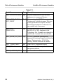
Table of Contents
TABLE OF CONTENTS
About This Manual
Related Publications
Simulation Manuals
Modeling Manuals
Falcon Framework Manuals
Chapter 1
Overview of QuickSim II
What is Simulation?
Why Simulate?
QuickSim II Overview
How QuickSim II Fits Into the Idea Station
QuickSim II Design Flow
QuickSim II Data Flow
Simulator Architecture
Input and Output Data
Chapter 2
Key Concepts
Electronic Designs
Design Viewpoints and QuickSim II
Design Evaluation and Model Selection
Managing Designs
Design Properties and Simulation
QuickSim II Logic Values and Drive Strengths
Simulator Accuracy
Logical Accuracy
Timing Accuracy
How QuickSim II Processes Circuit Activity
What is Circuit Activity?
The Timing Wheel
The Scheduling Algorithm
Simulation Timing Modes
QuickSim II User's Manual, V8.5_1
xiii
xiv
xvi
xvi
xvii
1-1
1-1
1-3
1-3
1-5
1-6
1-10
1-12
1-14
2-1
2-2
2-4
2-6
2-8
2-9
2-9
2-11
2-11
2-12
2-13
2-14
2-14
2-16
2-19
iii
Table of Contents
TABLE OF CONTENTS [continued]
Delay Scaling
Delay Modes
Spike Models
Conditions that Cause a Spike
Simulator Spike Models
Technology File Configurable Spike Models
Netdelay Property Spike Model
Spike Model Simulation
Spike Message Reporting
Waveform Databases
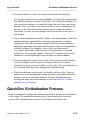
QuickSim II Initialization Process
Default Initialization
Classic Initialization
Suppressing Warnings During Initialization
Design Changes in QuickSim II
Effects of Design Changes
Reloading Models
Swapping Models
Changing Properties
Back Annotation Objects and QuickSim II
EDDM Bundle Functionality
Hierarchical Pin Keep Functionality
SDF in QuickSim II
The QuickSim Load SDF File Command
Importing an SDF file Using TimeBase
Chapter 3
Operating Procedures
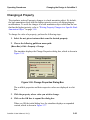
Processing a Design For Simulation
Invoking QuickSim II
Invoking from the Design Manager
Invoking from A Shell
Running a Batch Simulation
Using Redirected Input
Using Here Documents
iv
2-21
2-21
2-24
2-24
2-25
2-28
2-30
2-30
2-36
2-37
2-39
2-40
2-41
2-41
2-42
2-43
2-46
2-47
2-47
2-48
2-49
2-49
2-50
2-50
2-51
3-1
3-3
3-6
3-6
3-10
3-11
3-11
3-12
QuickSim II User's Manual, V8.5_1
Table of Contents
TABLE OF CONTENTS [continued]
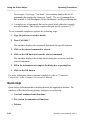
Exiting and Suspending the Simulator
Using the Online Helps
Command Completion
Quick Help
Reference Help
Setting Up QuickSim II
Setting Up the Kernel
Setting Up Instance By Instance
Initializing the Design
Suppressing Initialization Warnings
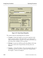
Saving Setup Conditions
Restoring Setup Conditions
Setting Timing Modes
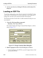
Loading an SDF File
Checking for Design Constraints
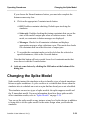
Changing the Spike Model
Checking for Spike Conditions
Changing the Contention Model
Checking for Contention
Checking for Hazard Conditions
Displaying Model Messages
Reporting Model Statistics
Gathering Toggle Statistics
Reporting Toggle Statistics
Checking Device Stability
Keeping Circuit Activity
Applying Stimulus to a Simulation
Using the Palettes
Running the Simulator
Resetting the Simulator
Saving and Restoring Simulation States
Using Breakpoints
Adding Breakpoints
Reporting Breakpoints
Deleting Breakpoints
QuickSim II User's Manual, V8.5_1
3-13
3-15
3-15
3-16
3-17
3-17
3-18
3-23
3-24
3-25
3-27
3-31
3-33
3-36
3-37
3-39
3-42
3-44
3-48
3-49
3-51
3-52
3-54
3-56
3-58
3-60
3-62
3-64
3-65
3-65
3-67
3-71
3-71
3-75
3-76
v
Table of Contents
TABLE OF CONTENTS [continued]
Back-tracing X States
Changing the Design in QuickSim II
Reloading A Model
Writing Property Changes to a Specific Back Annotation Object
Swapping A Model
Changing A Property
Chapter 4
Operating Procedures Cross-Index
4-1
Common Simulation Interface Procedures
Design Viewing and Analysis Support (DVAS) Procedures
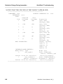
Design Viewpoint Editor Procedures
Appendix A
QuickSim II Troubleshooting
4-1
4-3
4-5
A-1
Quicksim II Debugging Tips
Quicksim Invocation Fails
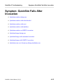
QuickSim Fails After Invocation
Symptom: Invoke Fails
QuickSim Crash During Invoke
QuickSim Crashes During Invoke with Reference to “ld.so”
QuickSim Crashes During Invoke with Reference to “__cb_bt”
QuickSim Crashes During Invoke with X
Quicksim II Hangs During Invocation
Problem Scenario:
Possible Solutions:
EXAMPLE:
SOLUTION
QuickSim Crash During Invoke with the Fault/Recovery Window
Signal 4 Recovery
General Instructions for “nulling” a Model (TAN 6229)
Signal 10 Recovery
The scenarios causing Signal 10 failures are:
Signal 11 Recovery
vi
3-77
3-78
3-78
3-80
3-81
3-83
A-1
A-1
A-1
A-2
A-3
A-4
A-5
A-6
A-7
A-7
A-7
A-7
A-9
A-11
A-12
A-12
A-13
A-13
A-14
QuickSim II User's Manual, V8.5_1
Table of Contents
TABLE OF CONTENTS [continued]
The scenarios known to cause Signal 11 failures are:
Signal 13 Error Message
Symptom: Memory Fault
Error Messages Issued
Cannot Connect to Child
Too Many Net Recursions
Parameter Undefined, TSUD
QuickSim Issues Warning Message on Invoke
QuickSim “NULLs” Model on Invoke
QuickSim Loads Wrong Models on Invoke
QuickSim Runs Out of Memory During Invoke
Symptom: QuickSim Fails After Invocation
Quicksim crashes during run
Quicksim crashes with reload model
Quicksim crashes with reset
Quicksim crashes with initialize
Quicksim crashes on AMPLE execution
Quicksim hangs during run
Quicksim hangs with command execution
Quicksim hangs with AMPLE execution
Quicksim runs out of memory during simulation run
Appendix B
Invocation of QuickSim II for FPGAstation
Introduction
Description of Functionality
Appendix C
QuickSim II Environment Variables
Introduction
Table of Environment Variables
QuickSim II User's Manual, V8.5_1
A-14
A-15
A-16
A-17
A-18
A-19
A-20
A-21
A-22
A-23
A-24
A-25
A-26
A-27
A-28
A-29
A-30
A-31
A-32
A-33
A-34
B-1
B-1
B-1
C-1
C-1
C-1
vii
Table of Contents
TABLE OF CONTENTS [continued]
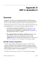
Appendix D
SDF in QuickSim II
D-1
Overview
OVI SDF Versions Supported
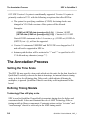
The Annotation Process
Setting the Time Scale
Defining Timing Models
The Role of the Timing Cache
Making SDF Annotations Persistent
Conflicts between SDF and other Database Changes
Annotating Specific Timing Modes
SDF/Technology File Correlation
Correlating Instance Paths
The AMP Timing Model
SDF CELL Templates
Correlating an SDF Statement with a Technology File Statement
D-1
D-1
D-2
D-2
D-2
D-3
D-4
D-5
D-6
D-7
D-7
D-8
D-8
D-8
Index
viii
QuickSim II User's Manual, V8.5_1
Table of Contents
LIST OF FIGURES
Figure 1. Simulation Documentation Roadmap
Figure 1-1. IDEA Tool Set
Figure 1-2. QuickSim II Design Flow
Figure 1-3. QuickSim II Data Flow
Figure 1-4. Architecture of QuickSim II
Figure 1-5. QuickSim II Input
Figure 1-6. QuickSim II Output
Figure 2-1. An Electronic Design
Figure 2-2. Model Selection Flow Chart
Figure 2-3. Simple Events
Figure 2-4. Timing Wheel
Figure 2-5. How the Simulator Sees the Schematic
Figure 2-6. Scheduling Events
Figure 2-7. Timing Mode Comparison
Figure 2-8. Inertial and Transport Delay Modes
Figure 2-9. X Duration for Spikes with Two tPX Transitions
Figure 2-10. X Duration for Spikes with One tPX Transition
Figure 2-11. Spike Pulse Propagation Regions
Figure 2-12. Single Output Device Spike Example
Figure 2-13. Pulse in Suppress Region: t2-t1 < suppress limit
Figure 2-14. X-pulse Region: suppress_limit <= t2-t1 < x_limit
Figure 2-15. Pulse in X-pulse Region: X-immediate is Specified
Figure 2-16. Pulse in Transport Region: X_limit < t2-t1 <= d1
Figure 2-17. Spike with Previous Event Scheduled
Figure 2-18. Scheduling Multiple Spike Models
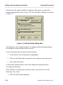
Figure 3-1. Design Manager Session Window
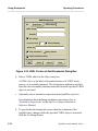
Figure 3-2. QuickSim II Dialog Box
Figure 3-3. Exit QuickSim Dialog Box
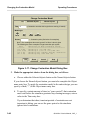
Figure 3-4. Setup Analysis Dialog Box
Figure 3-5. Expanded Setup Analysis Dialog Box
Figure 3-6. Change Timing Mode Dialog Box
Figure 3-7. INIT Prompt Bar
Figure 3-8. Change Warning Start Dialog Box
Figure 3-9. Change Warning Start User-Specifications
Figure 3-10. Save Setup Dialog Box
ix
xv
1-5
1-7
1-10
1-12
1-14
1-16
2-2
2-7
2-14
2-15
2-16
2-18
2-19
2-22
2-27
2-27
2-28
2-30
2-31
2-33
2-33
2-34
2-35
2-36
3-7
3-9
3-14
3-20
3-22
3-24
3-25
3-26
3-26
3-28
QuickSim II User's Manual, V8.5_1
Table of Contents
LIST OF FIGURES [continued]
Figure 3-11. Restore Setup Dialog Box
Figure 3-12. Change Timing Mode Dialog Box
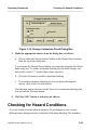
Figure 3-13. Change Constraint Mode Dialog Box
Figure 3-14. Change Constraint Mode Dialog Box
Figure 3-15. Change Spike Model Dialog Box
Figure 3-16. Change Spike Warnings Dialog Box
Figure 3-17. Change Contention Model Dialog Box
Figure 3-18. Change Contention Check Dialog Box
Figure 3-19. Change Hazard Check Dialog Box
Figure 3-20. Change Model Messages Dialog Box
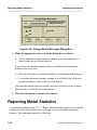
Figure 3-21. Report Model Statistics Dialog Box
Figure 3-22. Change Toggle Check Dialog Box
Figure 3-23. Report Toggle Dialog Box
Figure 3-24. Change Stability Check Dialog Box
Figure 3-25. Setup Palette
Figure 3-26. Reset Dialog Box
Figure 3-27. Save State Dialog Box
Figure 3-28. Restore State Dialog Box
Figure 3-29. Add Breakpoint Dialog Box
Figure 3-30. VHDL Portion of Add Breakpoint Dialog Box
Figure 3-31. Breakpoints Report Window
Figure 3-32. Delete Breakpoints Dialog Box
Figure 3-33. Reload Model Dialog Box
Figure 3-34. Specifying a Model
Figure 3-35. Change Model Dialog Box
Figure 3-36. Change Properties Dialog Box
Figure 3-37. Expanded Change Property Dialog Box
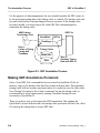
Figure D-1. SDF Annotation Process
Figure D-2. Twelve to Six Rvalue Transform
Figure D-3. Six to Three Rvalue Transform
Figure D-4. Six to Two Rvalue Transform
x
3-32
3-35
3-36
3-38
3-41
3-43
3-46
3-49
3-50
3-52
3-53
3-55
3-57
3-59
3-64
3-66
3-69
3-70
3-72
3-74
3-75
3-76
3-79
3-80
3-82
3-83
3-84
D-4
D-22
D-23
D-23
QuickSim II User's Manual, V8.5_1
Table of Contents
LIST OF TABLES
Table 2-1. Functional Model Types
Table 2-2. Simulation State Values
Table 2-3. QuickSim II Node Resolution
Table 3-1. Circumstances that Suggest a Custom Setup
Table 3-2. System Setup Groups
Table 4-1. Operating Procedures in the
SimView Common Simulation User’s Manual
Table 4-2. Operating Procedures that are found in the
Design Viewing and Analysis Support Manual
Table 4-3. Operating Procedures that are found in the
Design Viewpoint Editor User’s and Reference Manual
Table C-1.
Table D-1. Mapping SDF Edge Specifiers
Table D-2. SDF Transition priority
Table D-3. Technology File to SDF 12-Value Data Field
QuickSim II User's Manual, V8.5_1
2-3
2-10
2-12
3-19
3-29
4-1
4-3
4-5
C-1
D-15
D-16
D-19
xi
Table of Contents
LIST OF TABLES [continued]
xii
QuickSim II User's Manual, V8.5_1
About This Manual
About This Manual
This manual explains how to use the QuickSim II application. QuickSim II is an
interactive logic simulator that allows you to verify Mentor Graphics electronic
designs. This manual provides background information, various simulation
procedures, and hyperlinked lists of related procedures. The audience for this
manual is design engineers who use Mentor Graphics applications to analyze the
performance and behavior of electronic circuitry models. For related information
about SimView/UI, which is the user interface for all Mentor Graphics simulators,
refer to the SimView Common Simulation User's Manual.
Before using this manual online, you should be familiar with the BOLD Browser.
The chapters “Overview of QuickSim II” and “Key Concepts” provide
background information about QuickSim II and digital simulation. The chapter
“Operating Procedures” contains procedures for commonly performed tasks. The
chapter “Operating Procedures Cross-Index” provides several lists of related
procedures that are documented in other manuals, and each procedure is a
hyperlink to the corresponding section in the appropriate manual.
For information about the documentation conventions used in this manual, refer to
Mentor Graphics Documentation Conventions.
QuickSim II User's Manual, V8.5_1
xiii
Related Publications
About This Manual
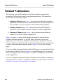
Related Publications
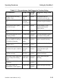
The following text and illustration lists the Mentor Graphics manuals that
document all of the features used by simulation applications. The manuals are
divided into the following categories:
• Simulation Manuals (page -xvi) -- these document individual simulation
applications and closely-related functionality that is common among two or
more simulators, such as viewpoint creation and charting capability.
• Modeling Manuals (page -xvi) -- these document the methodologies
available to create models for Mentor Graphics simulation applications.
• Framework Manuals (page -xvii) -- these document features that are
common to all Mentor Graphics applications.
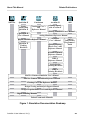
Figure 1 on page -xv shows which manuals document the various Mentor
Graphics simulation products. To use this figure, locate the icon for your
application across the top row and then descend along the shaded bar. This bar
overlaps each document title box that contains information about your application.
For more information about manuals listed in Figure 1, refer to the following
pages.
If you are reading this manual online in the Bold Browser, you can click the Select
mouse button on the title boxes in Figure 1 to open that document. You can also
click on an application icon in the top row to open the Getting Started workbook
for that application.
If you are unfamiliar with general Mentor Graphics documentation conventions or
need to know how to write a command or a function, you should first read Mentor
Graphics Corporation Documentation Conventions.
xiv
QuickSim II User's Manual, V8.5_1
About This Manual
SimView
Related Publications
QuickSim II
Continuum
AccuSim II
Getting
Started with
QuickSim II
Continuum User’s
and
Reference Manual
Getting Started
with AccuSim II
QuickSim II
User’s Manual
AIK
Analog Simulators User’s Manual
Analog Simulators Reference Manual
Digital Simulators Reference Manual
QuickSim II
Training
Workbook
AccuParts
User’s Manual
System Modeling
Blocks User’s and
Reference Manual
Analog
Interface Kit
Programmer’s
Guide
AccuSim II Models
Reference Manual
HDL-A
Reference Manual
Analog Station
Training Workbook
HDL-A
Training Workbook
SimView Common Simulation User's Manual
SimView Common Simulation Reference Manual
Charting User's and Reference Manual
Design Viewing and Analysis Support Manual
Design Viewpoint Editor User's and Reference Manual
Digital Modeling Manuals
Falcon Framework Manuals
Figure 1. Simulation Documentation Roadmap
QuickSim II User's Manual, V8.5_1
xv
Related Publications
About This Manual
Simulation Manuals
Design Viewing and Analysis Support Manual contains information about Design
Viewing and Analysis Support (DVAS). DVAS consists of functions and
commands that provide selection, viewing, highlighting, reporting, grouping,
syntax checking, naming, and window-manipulating capabilities.
Design Viewpoint Editor User's and Reference Manual contains information
about the Design Viewpoint Editor (DVE). DVE allows you to add, modify, and
manage back annotation data, as well as define and modify design configuration
rules for design viewpoints.
Fault Analysis User's Manual contains overview information and fault analysis
operating procedures relating to the QuickGrade II and QuickFault II fault
analysis applications.
SimView Common Simulation Reference Manual contains information about the
commands, functions, userware, and related reference material for the SimView
application. This material is also common to all Mentor Graphics digital and
analog analysis applications.
SimView Common Simulation User's Manual describes how to use the SimView
application. This manual provides background information, various simulation
procedures, and a comprehensive list of related procedures that are common to all
Mentor Graphics digital and analog analysis applications.
Modeling Manuals
Behavioral Language Model (BLM) Development Manual describes how to use
the files, commands, and data structures available with Mentor Graphics software
to write BLMs.
Digital Modeling Guide contains an overview of all digital modeling techniques
and their trade-offs.
Getting Started with System-1076 is for digital design engineers who have not
previously used System-1076. This training workbook provides basic instructions
xvi
QuickSim II User's Manual, V8.5_1
About This Manual
Related Publications
for using System-1076 to create and use VHDL models in the Mentor Graphics
environment.
Memory Table Model Development Manual contains information that helps you
develop Memory Table Models, which specify the functionality of a memory
device's pins.
Properties Reference Manual contains comprehensive information about Mentor
Graphics design properties, which are used by many Mentor Graphics products,
including all simulation applications.
QuickPart Schematic Model Development Manual contains information that helps
you develop QuickPart Schematic models. These types of models are based on a
compiled schematic.
QuickPart Table Model Development Manual contains information that helps you
develop QuickPart Table models. These types of models are based on ASCII truth
tables.
System-1076 Design and Model Development Manual provides concepts,
procedures, and techniques for using VHDL within the System-1076
environment.
Technology File Development Manual explains the use of technology files to aid
in the modeling of electronic parts and components. This manual provides
detailed reference information about technology file statements, usage
information, and a tutorial.
Falcon Framework Manuals
AMPLE User's Manual describes how to use the Mentor Graphics AMPLE
language. This manual contains flow-diagram descriptions and explanations of
important concepts, and shows how to write AMPLE functions.
BOLD Browser User's Manual explains basic BOLD Browser operations such as
searching for a phrase in the INFORM library, using the travel log, and following
hypertext links to view different documents. The BOLD Browser provides access
to reference help for most Mentor Graphics applications.
QuickSim II User's Manual, V8.5_1
xvii
Related Publications
About This Manual
Common User Interface Manual describes how to use the user interface features
that are common to all Mentor Graphics products. This manual tells how to
manage and use windows, the popup command line, function keys, strokes,
menus, prompt bars, and dialog boxes.
Customizing the Common User Interface describes how to extend the Common
User Interface. This manual explains how to redefine keys and how to create your
own menus, windows, dialog boxes, messages, and palettes.
Design Manager User's Manual provides information about the concepts and use
of the Design Manager. This manual contains a basic overview of design
management and of the Design Manager, key concepts to help you use the Design
Manager, and many design management procedures.
Getting Started with Falcon Framework is for new users of the Mentor Graphics
Falcon Framework. This workbook introduces you to the components of the
Falcon Framework and provides information about and practice using the
Common User Interface, Design Manager, INFORM, Notepad, and Decision
Support System applications.
Notepad User's and Reference Manual describes how to edit files and documents
in Notepad, a text editor. This manual provides examples, explanations, and an
alphabetical listing of AMPLE functions that are available for customizing
Notepad.
xviii
QuickSim II User's Manual, V8.5_1
Chapter 1
Overview of QuickSim II
This chapter provides important background information about QuickSim II. This
background information can help you to use QuickSim II effectively. This chapter
contains the following sections:
What is Simulation?
1-1
Why Simulate?
1-3
QuickSim II Overview
How QuickSim II Fits Into the Idea Station
QuickSim II Design Flow
QuickSim II Data Flow
Simulator Architecture
Input and Output Data
1-3
1-5
1-6
1-10
1-12
1-14
What is Simulation?
Simulation is the modeling, exercising, and behavior analysis of an electronic
design without the ownership costs of the physical hardware. QuickSim II
calculates the behavior of a design and provides useful displays that you can use
for analyzing the behavior. It provides a reality check that gives you confidence in
your design work.
To analyze an electronic design, you must either have the design physically
available or a representative model whose behavior can be simulated. If you use a
representative model, it must have all the attributes of the physical design and the
test bench environment.
Because QuickSim II allows different types of models, you can use it all the way
through your design process. During functional simulation, which happens early
QuickSim II User's Manual, V8.5_1
1-1
What is Simulation?
Overview of QuickSim II
in the design process, you typically focus on analyzing and debugging high-level
functional models. As you develop the detailed description of your design, you
can use the modeling method that best suits your objectives and still use the same
simulator.
The attributes of a practical digital logic simulator are accuracy, efficiency, and
comprehensiveness. Accuracy means a close correspondence between simulated
signal values over time and the behavior of the physical design. Efficiency refers
to workstation memory requirements and simulation speed. Comprehensiveness
refers to the degree to which the simulator manages a broad class of digital
designs independent of device technologies.
A simulator should manage the many types of bipolar and MOS designs,
including the following:
• Standard digital logic configurations, such as the following:
o Combinational circuits (logic networks with no storage capability)
o
Synchronous circuits (any clocked device)
o Asynchronous circuits (any unclocked sequential circuit with feedback)
• A wide selection of model types, such as the following:
o Switch-level transistor models (unidirectional and bidirectional)
o Gate-level models (AND, NAND, OR, and so on)
o Sequential models (latches and registers)
o Functional models (compiled from gate-level or state table models)
o Special models (ROMs, RAMs, PLAs, PLDs, one-shots, and multi-
vibrators)
o VHDL models
o Hardware (physical) models
1-2
QuickSim II User's Manual, V8.5_1
Overview of QuickSim II
Why Simulate?
o Behavioral models (written in a standard high-level language)
o Technology description models
• Multiple states (logic 1, 0, and X (unknown)) and multiple strengths
(strong, resistive, high-impedance, and indeterminate)
• Timing modes (such as minimum, typical, and maximum timing values)
• Timing error checking, such as setup and hold
• Initialization and oscillation handling algorithms
• Tri-state and bidirectional modeling algorithms
Why Simulate?
Computer simulation of digital circuits has long been used to extend the range of
many types of analyses and to enable the analysis of larger and more complex
designs. This type of analysis, when performed prior to the prototype stage,
ensures the design's quality earlier in the engineering process, where errors are
easier and cheaper to fix.
With a simulator you can analyze the design as you would on the test bench, with
stimulus, probes, and waveform displays. The major benefit of the workstation is
integration of this analysis task with other phases of the development cycle: from
concept, to design, to analysis, to physical layout, to the manufacturing test
environment. With this improved productivity, design cycles can be considerably
shorter than with the classic methods of paper, pencil, breadboard, hand-layout,
and manual test program generation.
QuickSim II Overview
The QuickSim II logic simulator is a sophisticated computer program that allows
you to test a “software breadboard” of a digital hardware design. It is an
interactive logic simulator that allows you to verify the functionality of models of
electronic designs. QuickSim II has the following features:
QuickSim II User's Manual, V8.5_1
1-3
QuickSim II Overview
Overview of QuickSim II
• 12-state, timing-wheel simulator that can simulate technologies, such as
CMOS, TTL, ECL, and so on.
• Logic analyzer-type tracing that lets you graphically examine the logic
states of signals.
• Interactive control of the simulation that lets you control and observe the
state of any signal in the design. You can trace, list, monitor, stimulate, or
set breakpoints on any signal.
• An interface that is shared with other Mentor Graphics simulators and is
compliant with Motif standards to provide a common look and feel. This
visual interface is called SimView/UI.
• The ability to save setup conditions, stimulus, and particular states of the
simulation so that they can be restored at any time in the future.
• Incremental design capabilities that let you update modified design
components and change property values during the simulation, even if the
change affects the design's connectivity or timing. These incremental
design capabilities let you make a change and then resume the simulation
quickly.
• The ability to perform simulations with varying trade-offs of simulation
speed versus simulation accuracy to obtain peak efficiency.
• The use of all Mentor Graphics simulation modeling methods, which
allows you to use QuickSim II for simulation during all phases of
development.
• The ability to import Standard Delay File format (SDF) timing information
into a simulation. This allows considerable flexibility in timing annotation.
• The calculation of timing as a function of pin loading and environmental
effects (such as temperature, voltage, and process), as well as other
modeling capabilities.
With QuickSim II, you can apply stimulus to the design, run the simulation,
analyze the results, and modify the design based on those results. You can then
1-4
QuickSim II User's Manual, V8.5_1
Overview of QuickSim II
QuickSim II Overview
reset the simulator, optionally revise or apply more stimulus to the design (the
simulator maintains the original set of stimulus), and start the cycle over. When
the design functions correctly, you can save the stimulus and simulation results
directly with the design to promote consistent and reliable design management.
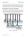
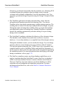
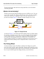
How QuickSim II Fits Into the Idea Station
Idea Station, which operates within the Falcon Framework, consists of a set of
tools that allow you to capture and analyze your design. The Falcon Framework
supports capture and analysis work, especially through design file management.
Figure 1-1 illustrates the simulator's role in the Idea Station tool set.
Falcon Framework
Schematic
Digital
Capture Simulation
QuickSim II
Design
Architect
SimView
Physical
Layout
Board
Station
Hardware
Modeling
Architectural
Modeling
LM Series
System-1076
Test
QuickGrade II
QuickFault II
Component Modeling
BLMs
QuickPart Schematic
QuickPart Table
Memory Table Model
Sheet-Based Parts
Figure 1-1. IDEA Tool Set
QuickSim II User's Manual, V8.5_1
1-5
QuickSim II Overview
Overview of QuickSim II
QuickSim II operates on a model of a digital logic circuit, which consists of parts
that you have connected together using design creation applications, such as
Design Architect.
Before you create your design, you need to obtain the parts that your design
requires. You can create your own parts using any of the component, architectural,
or hardware modeling techniques that QuickSim II supports. You can also use
parts from libraries provided by third-party vendors.
When your design simulates correctly, you can perform the physical layout, which
is supported by other Mentor Graphics tool sets. Or, if you are using a third-party
library, the library vendor might perform the layout. Data that is calculated during
design layout might include load-dependent delay values, which you can insert, or
back annotate, to the design for the final verification.
Before moving into your manufacturing processes, you can further analyze your
design using Mentor Graphics timing and test analysis applications. The
QuickPath static timing analyzer, the QuickGrade II fault grader, and the
QuickFault II fault simulator, which are optional Idea Station applications, help
determine your design's timing and testability requirements and performance.
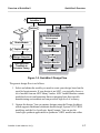
QuickSim II Design Flow
The flow through design creation and analysis is influenced by many factors, and
it can be unique for each development effort. A company's internal requirements
and use of external applications can dictate the tasks and the timing that the
developer must adhere to. Although there are many different design flows, some
generic tasks apply to almost all of them. Figure 1-2 illustrates a generic design
creation and simulation design flow.
1-6
QuickSim II User's Manual, V8.5_1
Overview of QuickSim II
QuickSim II Overview
Invoke
QuickSim II
5
System
SimView
Full Timing
Functionality
1
Obtain Models
2
Capture Design
3
Optionally Create
Design Viewpoint
4
Optionally Run
TimeBase to
Calculate Timing
Environment
A Set Up Simulation
Environment
Environment
Stimulus
B Generate/Refine
Stimulus
Stimulus
C
SimView
Run Simulation
SimView
SimView
D
Analyze Results
E
E. Modify Design
(optional)
Modify Design
Modify E.
Design
(optional)
(optional)
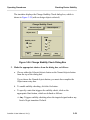
Figure 1-2. QuickSim II Design Flow
The generic design flow is as follows:
1. Select and obtain the models you need to create your design, based on the
specified requirements. If your design is an ASIC, you typically choose a
set of models from an ASIC library vendor. ASIC vendor libraries contain
predefined circuit configurations that are integrated into their specific
manufacturing environment and can provide a high level of accuracy.
2. Capture the design. You can capture designs using the Design Architect,
which supports traditional schematic-based design, System-1076 VHDL
modeling, and the five AutoLogic Input Formats. You can use the
AutoLogic synthesis application to synthesize VHDL models into either
QuickSim II User's Manual, V8.5_1
1-7
QuickSim II Overview
Overview of QuickSim II
netlists or gate representations, both of which are compatible in the
simulator.
For information about synthesizing VHDL models, refer to the AutoLogic
VHDL Synthesis Guide. For information about the AutoLogic Input
Formats, refer to the AutoLogic BLOCKS Manual.
3. Optionally, invoke the Design Viewpoint Editor (DVE) to create a
viewpoint that defines a custom configuration. For more information about
design viewpoints, refer to “Design Viewpoints and QuickSim II” on
page 2-4.
4. Optionally, run the TimeBase application to calculate the design's timing
values in batch mode before you invoke the simulator. For information
about the TimeBase application, refer to the chapter “Using TimeBase” in
the Technology File Development Manual.
5. Optionally, invoke SimView, which is a read-only simulator. SimView
allows you to view the design, and create and edit stimulus. For information
about SimView, refer to the SimView Common Simulation User's Manual.
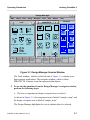
6. Invoke QuickSim II. If you used DVE to create a design viewpoint, you
should specify the design viewpoint when you invoke the simulator.
Otherwise, the simulator invokes on a design viewpoint that defines default
configuration rules, and it creates it in memory if it does not already exist.
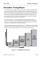
The typical strategy for simulation is an iterative process that has three
main phases: verify functionality without regard for timing, verify
functionality according to timing effects, and verify functionality once the
design is integrated into a higher-level system. Although the focus of each
phase is different, the tasks that you perform within the simulator are very
similar.
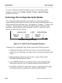
The typical flow within the QuickSim II application is as follows:
a. Set up the simulation environment. The simulation environment
consists of things such as the user interface, breakpoints for debugging,
timing mode, circuit violation checks, and the signal data that you want
maintained for analysis later.
1-8
QuickSim II User's Manual, V8.5_1
Overview of QuickSim II
QuickSim II Overview
You may want to establish a persistent version of your design, which
you can do by latching the design viewpoint. A latched viewpoint
maintains a specific version of your design and all the objects it
references, which allows you to simulate your design without dealing
with incremental changes until you are ready. You might also import
ASCII back annotation data to adjust the timing values that the
simulator calculates.
b. Generate and refine stimulus. Stimulus is input data that the simulator
uses to exercise the design. QuickSim II supports several methods for
creating and refining stimulus, such as commands, functions, graphical
waveform editor, logfiles, and the Mentor Interactive Stimulus
Language (MISL). All methods result in an efficient, compiled form
called a waveform database, which you can manipulate, edit, save, and
delete.
c. Run the simulation. You can optimize the simulator to either run fast or
produce highly accurate results. Speed is important for early debug
analysis. On the other hand, you can request a high level of accuracy to
verify the design before going into manufacturing.
d. Analyze the results of the simulation. You can use several types of
display windows to help you debug your design. For example, graphical
schematic displays help you view and traverse the hierarchy of your
design, waveform trace displays present waveform values and signal
relationships, and cross-window highlighting quickly leads you to
objects of interest. You can save the results data to analyze later or to
compare with other results.
e. Optionally modify the design. If you find a problem with the design or
you want to use an updated model, you can bring the changes directly
into the simulator without exiting first. For example, you can change
and recompile a VHDL model using the capabilities in the Design
Architect, reload the model in the simulator, and then continue with
your simulation without exiting and re-invoking the simulator.
QuickSim II User's Manual, V8.5_1
1-9
QuickSim II Overview
Overview of QuickSim II
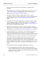
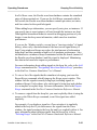
QuickSim II Data Flow
The data flow for QuickSim II involves several design data objects and several
applications. Figure 1-3 shows the data flow for QuickSim II.
1
Models
Design Architect
2
Electronic Design
SimView
6
Back
Annotation
SimView/UI
Waveform
Databases
SimView
Kernel
3
5
QuickSim II
Design
Viewpoint
Component
SimView/UI
QuickSim II
Kernel
4
TimeBase
Figure 1-3. QuickSim II Data Flow
• QuickSim II simulates electronic designs, and the first stage of the design
flow is to create a piece of the design called a component. The component
consists of the logical, graphical, timing, and technology aspects of the
design. You can use the schematic, symbol, and VHDL editing capabilities
of the Design Architect to create components. Once you have created the
component, you can move immediately into simulation.
• The design viewpoint contains the configuration rules that define how the
simulator perceives the component. The design viewpoint is essential to
simulation (and other applications). The configuration rules define design
and expression parameters, design viewpoint substitutions, and visible
properties. They also define the instances in the design that are primitive.
1-10
QuickSim II User's Manual, V8.5_1
Overview of QuickSim II
QuickSim II Overview
(Primitives provide the functionality that the simulator uses.) Running DVE
is optional because the simulator (upon invoking) creates a design
viewpoint with a default configuration if one does not already exist. You
can create specialized design viewpoints using the Design Viewpoint Editor
(DVE).
• The TimeBase application calculates unscaled delay values from the
information and equations provided in technology files. You can use
TimeBase when your design contains many complex timing equations. The
resulting data is cached in a data object and placed in the design viewpoint.
Having this cache of timing data available when you invoke the simulator
can significantly reduce invocation time. Running TimeBase is optional
because the simulator automatically calculates timing if no pre-existing
timing cache is available.
• The QuickSim II simulator calculates the behavior of the electronic design.
The simulator reads stimulus from (and writes results to) waveform
databases. A waveform database is a compiled form of the design's activity.
During the simulation session, you can modify the design. You can change
property values to correct design errors or to perform “what if” analysis.
You can also update technology files, VHDL source files, schematics, and
compiled models (such as QuickPart Tables and QuickPart Schematics). A
back annotation object stores the edits made to the associated design during
the simulation session. For more information about modifying your design
during a simulation, refer to page 3-78.
• The SimView simulator creates waveform databases and allows you to
analyze simulation data that QuickSim II creates. SimView is sometimes
called a read-only simulator because it cannot calculate circuit behavior.
However, SimView can create and save waveform databases as well as
setup data such as breakpoints and simulation expressions. For more
information about SimView, refer to the SimView Common Simulation
User's Manual.
QuickSim II User's Manual, V8.5_1
1-11
QuickSim II Overview
Overview of QuickSim II
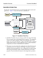
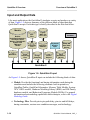
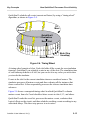
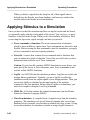
Simulator Architecture
The simulator consists of several major pieces of software. The pieces are
organized into an architecture that optimizes simulation efficiency and
performance. Figure 1-4 shows a representation of the simulator architecture.
QuickSim II
Session
Windows
$
doc
$
Front End
QuickSim II Userware
SimView/UI
(Common Sim
User Interface)
Keys
DVAS
DVE
DSC
Mouse
QuickSim II Kernel
Electronic
Design
Database
Waveform Databases
Figure 1-4. Architecture of QuickSim II
The following list defines the major elements of the simulator architecture:
• Front-End. Communicates with the user (through the session windows,
keys, and mouse), the design data, and the QuickSim II kernel.
1-12
QuickSim II User's Manual, V8.5_1
Overview of QuickSim II
QuickSim II Overview
• QuickSim II Userware. Consists of menus, key definitions, applications
windows, commands, and so on, that enhance the usability of the simulator.
• Common Simulation User Interface. Consists of a set of commands
(common to all Mentor Graphics simulators) that let you interact with the
simulation and display the simulation results for analysis.
• DVAS (Design Viewing and Analysis Support). Lets you select, view,
group, and report on design items.
• DVE (Design Viewpoint Editor). Lets you perform incremental design
changes during the simulation.
• SC (Simulation Checker). Lets you check simulation properties during the
simulation session. The SC is useful after making incremental design
changes.
• Electronic Design Database. Contains the design database, design
viewpoint, back annotations, and other design objects that the simulator
uses. This database provides information to both the front-end and the
kernel.
• QuickSim II Kernel. Performs the actual simulation by analyzing the
functional and timing models.
• Waveform Databases (WDBs). Provides the stimulus to the design and
holds the simulation results.
QuickSim II User's Manual, V8.5_1
1-13
QuickSim II Overview
Overview of QuickSim II
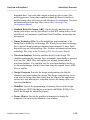
Input and Output Data
Like most applications, the QuickSim II simulator accepts and produces a variety
of data. Figure 1-5 shows a summary of the different kinds of input data that
QuickSim II accepts. Each data type is briefly described in the lists that follow.
Models
Builtins
QuickPart Schematics
QuickPart Tables
Memory Table Models
System-1076
LM-Family
BLMS
Modelfiles
SDF
Files
Logfile
MISL File
Force File
Technology
Files
Waveform
Database
Linear
Technology
Files
Design
Viewpoint
Environment
Variables
Keyboard/
Graphic
Input
Setup and
Save State
Objects
Back
Annotation
Objects
Picture
Objects
QuickSim II
Figure 1-5. QuickSim II Input
As Figure 1-5 shows, QuickSim II input can include the following kinds of data:
• Models. Provide the functional and timing information used during the
simulation and include the following elements: built-in primitives,
QuickPart Tables, QuickPart Schematics, Memory Table Models, System1076 VHDL models, Hardware Modeling Library (HML) and LM-Family
hardware models, and Behavioral Language Models (BLMs). For general
information about modeling capabilities and techniques, refer to the Digital
Modeling Guide.
• Technology Files. Provide pin-to-pin path delay, pin rise and fall delays,
timing constraints, custom error condition messages, and technology-
1-14
QuickSim II User's Manual, V8.5_1
Overview of QuickSim II
QuickSim II Overview
dependent data. You create and compile technology files as part of the
modeling process. Notice that compiled technology files are considered
models because they add to the overall definition of a component. For more
information about technology files, refer to the Technology File
Development Manual.
• Standard Delay File format (SDF). Can be directly annotated into the
timing.cache object used by QuickSim II so that SDF timing delays can be
used directly in a simulation. QuickSim II and TimeBase can annotate this
information.
• Linear Technology Files. Provide straight-line approximations of the
timing that is defined by a technology file. When you use linear technology
files, a typical design's timing is computed approximately 10 times faster
than when you use full technology files. For more information about linear
technology files, refer to the Technology File Development Manual.
• Waveform Database. Provides stimulus directly to the design. The
simulator automatically converts Force commands (individually or grouped
in a force file), MISL files, and logfiles into a binary format called a
waveform database. You can then save the waveform database and use it
for future simulations, which is faster than using the original forces, MISL
files, or logfiles.
• Design Viewpoint. Provides the design configuration rules that the
simulator uses when reading the design. The design viewpoint also serves
as an area for storing other data objects that are related to the application,
such as save state data objects, setup data objects, the timing cache, and
waveform databases.
• Modelfiles. Specify the programming of memory devices in the design.
Modelfiles are ASCII files that are associated with RAMs, ROMs, PLAs,
and PLDs through the Modelfile property.
• Picture Objects. Provide the graphical information to display the
schematic of a circuit in the schematic view window.
QuickSim II User's Manual, V8.5_1
1-15
QuickSim II Overview
Overview of QuickSim II
• Back Annotation Objects. Contain design property changes that were
made in tools other than the Design Architect. Back annotation objects are
attached to the design viewpoint.
• Setup Objects. Contain information about the simulator's initial setup
conditions. You can restore a setup to establish the same conditions that
you established in a previous simulation session.
• Save State Objects. Contain
Logfile
MISL File
Force File
information
about the simulator's state. You
can restore a saved state to establish the same point in a simulation that was
achieved in a previous session.
• Environment Variables. These are set in a command window or shell
prior to invoking QuickSim II. A list of environment variables used by
QuickSim II is described in Appendix C.
Figure 1-6 shows the types of output data that QuickSim II can produce.
QuickSim II
Display
Window
Report Files
Design
Viewpoint
Waveform
Database
Logfile
or
Stimulus
Window
Plots
Setup and
Save State
Objects
RAM/ROM
Files
Back
Annotation
Objects
Force File
Figure 1-6.
QuickSim II Output
The simulator's output can include the following kinds of data:
• Display. Shows you the simulation waveforms and logic state values. To
save time, you can omit the display by using the -Nodisplay switch when
you invoke the simulator. You might use the -Nodisplay “batch” approach
1-16
QuickSim II User's Manual, V8.5_1
Overview of QuickSim II
QuickSim II Overview
when simulating a large design. Instead of displaying the results
immediately, you can store them in either a waveform database or a logfile
and view them later.
• Design Viewpoint. Defines the design configuration rules and holds design
viewpoint related data, such as the simulation timing cache, waveform
databases, logfiles, save state and setup objects, and connections to back
annotation objects.
• Window Report Files. Contain ASCII representations of text-based
windows such as the List, Breakpoints, Waveforms, and Transcript
windows.
• Waveform Database. Contains waveform data that was stored in memory.
In-memory waveform databases include the Results, Stimulus, and Forces
waveform databases (all three are created and maintained by the simulator),
and any waveform database that you have previously loaded into memory.
• Logfile. Contains simulation results in ASCII format. You can create
logfiles from the contents of any loaded (in-memory) waveform database.
Logfile contents and syntax is described in “Simulation Logfiles” in the
SimView Common Simulation Reference Manual.
• Force File. Contains Force commands. The simulator can create a force file
from the waveforms in waveform databases (such as either the Forces or the
Stimulus waveform database).
• Setup Objects. Contain information about the simulator's initial setup
conditions. You can save these in the design viewpoint container to
maintain a strong association to your simulation.
• Save State Objects. Contain information about the simulator's state. You
can save these in the design viewpoint container to maintain a strong
association to your simulation.
• RAM/ROM Files. Contain the current contents of a RAM or ROM in the
design. These ASCII files are produced by the Write Modelfile command,
and are represented in modelfile format.
QuickSim II User's Manual, V8.5_1
1-17
QuickSim II Overview
Overview of QuickSim II
• Window Plots. Contain window data printed by the specified printer. For
example, you can plot Trace windows.
• Back Annotation Objects. Contain changes to the design that were made
in tools other than the Design Architect. For example, when you change a
property within QuickSim II, the change is added to the back annotation
object. For more information about back annotation objects, refer to “Back
Annotation Objects and QuickSim II” on page 2-48.
The next chapter describes the key concepts that pertain to QuickSim II and to
digital logic simulation.
1-18
QuickSim II User's Manual, V8.5_1
Chapter 2
Key Concepts
This chapter contains the following sections:
Electronic Designs
2-2
Design Viewpoints and QuickSim II
2-4
Design Evaluation and Model Selection
2-6
Managing Designs
2-8
Design Properties and Simulation
2-9
QuickSim II Logic Values and Drive Strengths
2-9
Simulator Accuracy
2-11
How QuickSim II Processes Circuit Activity
2-13
Simulation Timing Modes
2-19
Delay Scaling
2-21
Delay Modes
2-21
Spike Models
2-24
Waveform Databases
2-37
QuickSim II Initialization Process
2-39
Design Changes in QuickSim II
2-42
SDF in QuickSim II
2-50
QuickSim II User's Manual, V8.5_1
2-1
Electronic Designs
Key Concepts
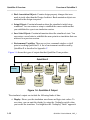
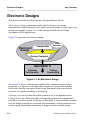
Electronic Designs
This section contains brief descriptions of design database objects.
An electronic design (sometimes simply called a design) is a software
representation of an electronic device, which can be as simple as a logic gate or as
complex as an entire system. You create a design with Electronic Design
Automation (EDA) applications.
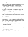
Figure 2-1 represents an electronic design.
Electronic
Design
Components
Back
Annotation
Design Viewpoint
QuickSim II
Symbols
Functionality
Timing
Connectivity
Figure 2-1. An Electronic Design
As Figure 2-1 shows, a design must include both a component and a design
viewpoint. A component is an object that contains a set of associated models.
Each model describes an aspect of the design: functional (which can include
connectivity), graphical, timing, or technology.
A design viewpoint is a data object that contains a set of configuration rules.
Configuration rules define the kinds of design information that an application
must have to perform its job. In the case of QuickSim II, this information includes
how the design elements are connected, the functionality of the modeled devices,
and the signal relationships and timing. A design can have multiple design
2-2
QuickSim II User's Manual, V8.5_1
Key Concepts
Electronic Designs
viewpoints, but the digital analysis applications typically use the same one. Also,
a design viewpoint can reference one or more back annotation objects. Back
annotation objects contain changes to the design that were made in tools other
than the Design Architect. For example, when you change a property within
QuickSim II, the change is added to the back annotation object.
You can create the technology and timing aspects of the design using models
called technology files (or linear technology files), with which you can build
sophisticated pin-to-pin timing delays and dependencies. You create the
component's graphical representation (which is called a symbol) using the Symbol
Editor in the Design Architect.
You can use a variety of methods to create functional models; each method you
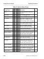
choose impacts the success of your design. Table 2-1 lists the methods available
for representing functional models. For information about selecting the best
modeling method for a given purpose, refer to the Digital Modeling Guide.
Model Type
Table 2-1. Functional Model Types
Description of Design Data Object
Behavioral Language The object file that results from your compiling a highModel (BLM)
level language source file that describes a device.
Builtin Model
An understanding of the device's logical behavior that
is built into the QuickSim II analysis tool.
Logic Model (LM)
The “Shell Software” and the physical device used with
the LM-Family hardware modelers.
QuickPart Schematic
Model
The object file that results from your compiling a
schematic with the QuickPart Schematic compiler.
QuickPart Table
Model
The object file that results from your compiling a
QuickPart Table file, which are ASCII files that
describe the different states of a device based on its
input and output pins.
Memory Table Model The object file that results from your compiling an
ASCII interface file that describes the memory access
control logic and actions of a memory array device.
QuickSim II User's Manual, V8.5_1
2-3
Design Viewpoints and QuickSim II
Model Type
Key Concepts
Table 2-1. Functional Model Types
Description of Design Data Object
Schematic Model
A schematic that you create with the Design Architect
by instantiating and connecting various models.
VHDL Model
The object files that result from your compiling with
the Design Architect VHDL Editor.
Each occurrence, or instance, of a component on a schematic sheet can consist of
a graphical model (the symbol), a functional model (its logic behavior), and a
technology model (process and implementation details). When you create the
component, you must associate these different aspects if you want the simulator to
use each aspect during a simulation. By default, the Design Architect and the
various model compilers create the appropriate associations for you; however, you
can explicitly associate models any way you want.
Because a component can have more than one version of each type of model, you
use labels to associate the models into an identifiable group. The simulator selects
the models that it uses during simulation according to how they are labeled. (The
value of the instance's Model property determines the labels that the simulator
selects.) For example, you could have several technology models, where each one
has a different label and describes a different set of process requirements. If the
associated graphical model has all of these labels, it could be grouped with any of
the technology models for any given instance. This ease of association provides
flexibility. For more information about how QuickSim II selects models, refer to
“Design Evaluation and Model Selection” on page 2-6.
For more information about how to register and label models, refer to “DA Model
Registration” in the Design Architect User's Manual.
Design Viewpoints and QuickSim II
A design viewpoint is a data object that performs two functions: it defines the set
of configuration rules that the simulator uses to evaluate the design, and it serves
as a container object in which information related to the simulation can be
managed. A design configuration can define four categories of rules:
2-4
QuickSim II User's Manual, V8.5_1
Key Concepts
Design Viewpoints and QuickSim II
• Parameter. The value of a design-based variable that is resolved outside of
the component. For example, you can use parameters to define bus widths
so that the design can be configured appropriately for different uses.
• Primitive. An instance that is a termination point for evaluation. Primitive
instances must provide device functionality to the simulator.
• Substitute. A property name whose value is to be substituted for another
property's value.
• Visible property. A property that is visible to DFI and netlisters.
The simulator can store the following related objects inside the design viewpoint
container:
• Save state object. Contains a complete kernel state (the values of all the
nets and instances in the design) at a specific point in simulation time. You
can restore a saved state to return the simulation to the point at which you
saved the state.
• Timing cache. Contains design viewpoint-specific timing information. The
timing cache is used only for full simulation timing; it is not used for unit
delay timing. Once the timing cache has been created, the simulator reuses
it until the version of the design viewpoint (or anything that the design
viewpoint references) changes.
• QuickSim setup object. Contains simulator setup conditions that you can
restore. Setup conditions include the kernel setup (timing and delay mode,
design and hierarchical checking modes and settings, and BLM checking),
the keep list, the run setup, and a list of breakpoint settings.
• SimView/UI setup object. Contains user interface setup conditions that
you can restore, including window positions and sizes, bus names,
synonyms, expressions, and user-loaded userware.
• Waveform databases. Contain compiled waveform data generated from
the simulation or through stimulus input.
QuickSim II User's Manual, V8.5_1
2-5
Design Evaluation and Model Selection
Key Concepts
A version freezing mechanism, called latching, allows you to maintain a specific
version of your design and all the objects it references. Design latching allows you
to stabilize the version of your design so you can simulate it without dealing with
incremental changes until you are ready. When you are ready to test the updated
version of the design, you can unlatch the old version. Then, the next time you
invoke the simulator, it brings in the newest version of each object that the design
references. To maintain the new version, you must again latch the design.
For detailed information about design viewpoints, configurations, and design
latching, refer to the Design Viewpoint Editor User's and Reference Manual.
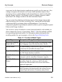
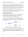
Design Evaluation and Model Selection
As the simulator invokes, it evaluates the design and selects the functional and
timing models to simulate. The following information controls how the simulator
evaluates the design and selects the simulation models:
• Model registration, labeling, and Model property values. When the
simulator locates a primitive instance, it matches the instance's Model
property to the component's registered labels and then selects the models
that the matching labels reference. For background information about labels
and model registration, refer to the “DA Model Registration” in the Design
Architect User's Manual.
• Configuration rules in the design viewpoint. The configuration rules
identify how far the simulator traverses the design hierarchy as it looks for
primitive instances. These rules can differ between a default configuration,
which the simulator creates, and a custom configuration, which you create
in the Design Viewpoint Editor.
2-6
QuickSim II User's Manual, V8.5_1
Key Concepts
Design Evaluation and Model Selection
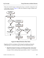
Before the simulator begins evaluating the design, it reads the configuration rules
in the design viewpoint. Figure 2-2 shows the simulator's design evaluation and
model selection process.
Begin Design
Evaluation
Get next instance
Primitive?
YES
NO
Get instance's
Model property
Match Model
property to labels
Is hierarchy NO
present?
YES
Descend to VHDL
or schematic
Successful YES
match?
NO
Insert a NULL
simulation model
Is model
valid for
simulation
?
YES
NO
Build representation
Figure 2-2. Model Selection Flow Chart
Beginning with the root instance of the design, the simulator performs the
following steps to evaluate the design and select the simulation models:
1. Beginning with the root instance, the simulator determines if the current
instance is a primitive according to the configuration rules in the design
viewpoint. In the resulting design representation, a slash (“/”) represents the
QuickSim II User's Manual, V8.5_1
2-7
Managing Designs
Key Concepts
root of the design. Note that an error occurs if the root of the design is a
primitive.
2. If the current instance is not defined as a primitive and it contains hierarchy,
the simulator descends to the lower level and starts the process over.
However, if the instance is not defined as a primitive and it does not contain
hierarchy, the simulator inserts a null model and starts the process over.
Null simulation models behave like an open circuit.
3. If the current instance is defined as a primitive, the simulator gets the
instance's Model property and attempts to match the value of the property to
the labels that are registered in the component interface. By order of
precedence, the simulator recognizes the following model specifiers:
• Specific labels, which are registered by users
• Labels that reference builtin simulation primitives
• Default labels, which are automatically registered by model compilers,
the Design Architect, and other design creation applications
4. If the Model property matches a label and the model that the label
references is valid for simulation, the simulator builds the internal
representation and starts the process over.
5. If either the Model property does not match a registered label or the
matched label does not reference a valid simulation model, the simulator
inserts a null simulation model and starts the process over. Again, null
simulation models behave the same as an open circuit.
Managing Designs
The Design Manager is an icon-based application that helps you manage your
designs. Within the Design Manager, you can directly invoke other Mentor
Graphics applications, as well as perform data management tasks such as copying,
moving, archiving, and releasing your design data. It also supplies a design data
navigator and a full set of self-explanatory icons for data representation. For more
2-8
QuickSim II User's Manual, V8.5_1
Key Concepts
Design Properties and Simulation
information about the Design Manager, refer to the Design Manager User's
Manual.
Design Properties and Simulation
A design property consists of a name and a value, and it helps describe model and
design characteristics for Mentor Graphics applications.
Properties help describe three schematic items: symbols, pins, and nets. A symbol
is a graphical representation of a component, a pin is the point that connects the
net to the circuitry represented by the symbol, and a net is a signal path that
connects two or more pins.
Examples of design characteristics that properties define are pin rise and fall
times, the initialization state of a pin or net, and the logic function associated with
a symbol body. Simulation design properties are discussed in the “Simulation
Design Properties” chapter of the Digital Simulators Reference Manual, and all
properties are described in the Properties Reference Manual.
QuickSim II Logic Values and Drive
Strengths
QuickSim II uses 12 signal states to simulate a logic circuit. A signal state
represents the electrical state of a signal. Each signal state is a combination of a
logic value and a drive strength. These signal states provide a comprehensive and
accurate approach to the simulation of logic designs.
The simulator uses three logic values: 0, 1, and X. The X value represents a logic
value that could be either 0 or 1, but cannot be reliably determined. During
simulation, X logic values can occur at design initialization as the simulator tries
to determine design “power-up” conditions. An X logic value can also be the
result of signal contention, which happens when two or more logic values are
driven simultaneously onto the same net.
Signal drive strengths allow the simulator to accurately resolve signal contention
and to simulate subtle effects of different design technologies. The simulator uses
QuickSim II User's Manual, V8.5_1
2-9
QuickSim II Logic Values and Drive Strengths
Key Concepts
four signal drive strengths: strong (S), resistive (R), high impedance (Z), and
indeterminate (I). (The I value represents a signal strength that could be either S,
R, or Z.) The simulator combines the signal drive strengths with the three logic
values to create the 12 signal states required for comprehensive and accurate
simulation of the different design technologies.
TTL designs typically require only five of these logic value/signal strength
combinations: 0 and 1 (for driving devices), X (for either 0 or 1, but you don't
know which), 1R (for pull-up resistors) and XZ (for any high-impedance signal
level). By substituting a 0R in place of the 1R, you can accurately model ECL and
its pull-down resistors.
The need to accurately model MOS designs at the transistor level led to the
indeterminate signal strength, enlarging the state-strength table to 12
combinations. Table 2-2 shows the resulting combination map that QuickSim II
uses.
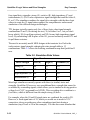
Table 2-2. Simulation State Values
Signal Level
Drive Strength
Low (0)
High (1)
Unknown (X)
Strong (S)
0S
1S
XS
Resistive (R)
0R
1R
XR
High Impedance (Z)
0Z
1Z
XZ
Indeterminate (I)
0I
1I
XI
Most logic simulators currently operate with these (or similar) states and
strengths. QuickSim II, however, uses an additional drive strength that cannot be
overridden by contending signals, which allows you to simulate a driving positive
voltage level (VCC) or ground level (GND). This overriding drive condition is a
fixed drive, which is different from the simple strong (S) drive.
For example, when the 1S and 0S signal states are combined, the result is XS.
However, a fixed signal state of 1S, which you would use to model a VCC
connection, always overrides any other contending signal state during a
simulation (stays 'fixed' at 1S in this example). You can also create stimulus that
2-10
QuickSim II User's Manual, V8.5_1
Key Concepts
Simulator Accuracy
has a fixed signal state, which is useful in debugging because it cancels the effects
of any driving output that is connected to the net.
Simulator Accuracy
The accuracy of a simulator can be measured in two ways: accuracy in the
verification of logical state-strength values and accuracy in timing.
Logical Accuracy
Logical accuracy is a direct function of the signal states that the simulator can
model. When more than one signal is connected to one net, the simulator must
have a means of determining an accurate result.
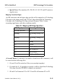
Table 2-3 (see page 2-12) is a matrix that describes how the simulator resolves
node contention between two or more output pins. To determine the state of a
node connected to the outputs of two gates, the simulator (figuratively) locates the
output state of one gate in the left-hand column and the output state of the other
gate in the top row; their cross-point indicates the state of the node.
When more than two outputs are connected, the simulator first separates the signal
states into two categories: signals of strengths S, R, or Z, and signals of strength I.
Then it calculates a single state for each category as follows: it plots the result of
two states from the same category, and then plots that result with another state in
the same category. It continues combining plotted results with output states until it
has a single state for each category, and then it calculates the actual state of the
node using the final values from each category.
For example, consider five connected output pins that have the following states:
0S, XI, XR, 1Z, and 0I. Using Table 2-3, the simulator would plot them as
follows:
1. First, it would separate the signal states into the two categories: [0S, XR,
and 1Z] and [XI and 0I].
2. Next, it would plot XR and 0S to yield 0S.
QuickSim II User's Manual, V8.5_1
2-11
Simulator Accuracy
Key Concepts
3. Then it would plot 0S (the result from step 2) and 1Z to yield 0S.
4. It would then plot XI and 0I to yield XI.
5. Last, it would plot 0S (the result from step 3) and XI (the result from step 4)
to yield XS, which is the actual state of the node.
0Z
0Z 0Z
XZ XZ
1Z XZ
0R 0R
XR XR
1R 1R
0I 0I
XI XI
1I XI
0S 0S
XS XS
1S 1S
NOTES:
1 :
X :
Z :
R :
S :
I :
Table 2-3. QuickSim II Node Resolution
XZ 1Z 0R XR 1R 0I XI 1I 0S
XZ XZ 0R XR 1R 0I
XI XI 0S
XZ XZ 0R XR 1R XI XI XI 0S
XZ 1Z 0R XR 1R XI XI 1I
0S
0R 0R 0R XR XR 0I
XI XI 0S
XR XR XR XR XR XI XI XI 0S
1R 1R XR XR 1R XI XI 1I
0S
XI XI 0I
XI XI 0I
XI XI 0S
XI XI XI XI XI XI XI XI XS
XI 1I
XI XI 1I
XI XI 1I
XS
0S 0S 0S 0S 0S 0S XS XS 0S
XS XS XS XS XS XS XS XS XS
1S 1S 1S 1S 1S XS XS 1S XS
XS
XS
XS
XS
XS
XS
XS
XS
XS
XS
XS
XS
XS
1S
1S
1S
1S
1S
1S
1S
XS
XS
1S
XS
XS
1S
0
:
Signal value of logic 0.
Signal value of logic 1.
Signal value is unknown (0 or 1).
Signal strength of high impedance.
Signal strength of resistive.
Signal strength of strong.
Signal strength of indeterminate.
Timing Accuracy
Timing accuracy in logic simulation is a function of three factors: the simulator's
basic unit of timing resolution, the attributes associated with the modeling
methods, and special compensation routines.
2-12
QuickSim II User's Manual, V8.5_1
Key Concepts
How QuickSim II Processes Circuit Activity
The basic unit of time resolution for QuickSim II is the timestep, which is user set
and which defaults to 0.1nS when the simulator is invoked. QuickSim II uses
timestep increments to model the passing of time during a simulation run. All
simulation activity occurs within timestep boundaries. The smaller the timestep,
the greater the timing resolution.
Modeling attributes help describe some of the real-world timing characteristics of
components. You typically develop modeling attributes during the schematicentry phase of the design process. Examples of the modeling attributes include the
following:
• Minimum, typical, and maximum timing for rising and falling signals on
inputs and outputs (inertial delay)
• Minimum, typical, and maximum pin-to-pin timing, which is defined in
technology files
• Setup, hold, skew and minimum pulse width timing checks, and clock
frequency constraints
• Timing constraint violations that affect output pin states
• Timing as a function of pin loading and simulated physical effects
• Transport delays for HML, LM-Family models, and QuickPart Schematics
(but not for QuickPart Tables)
Compensation routines annotate the timing of a design with load-dependent delay
estimates from physical layout data, process variation data, as well as temperature
and voltage variances.
How QuickSim II Processes Circuit
Activity
Understanding how the simulator processes a simulation can help you use it more
efficiently. The following text describes the type of circuit activity that the
simulator processes and demonstrates how it schedules the activity for processing.
QuickSim II User's Manual, V8.5_1
2-13
How QuickSim II Processes Circuit Activity
Key Concepts
The discussion begins with some basic concepts and then covers the detailed
scheduling algorithm.
What is Circuit Activity?
The basic circuit activity that the simulator processes is called an event. An event
occurs when a signal's state changes (either the logic value or the drive strength),
which can be caused by a component's output or by input stimulus that you
provide to the design. Figure 2-3 illustrates a simple example of two events.
QuickSim II
Evaluates
Buffer
Mature Event
t
Event Scheduled
t+7
OUT
IN
7
9
Figure 2-3. Simple Events
As shown in Figure 2-3, the input to the buffer changes from low to high, causing
the simulator to schedule an event. The event is like a flag that tells the simulator
it must evaluate the buffer. The simulator evaluates the buffer according to the
new input state, and propagates the newly evaluated state of the buffer to its
output, resulting in another event. When the simulator processes this last event, it
typically fans out the resulting value to components that are connected to the
output.
The Timing Wheel
Accurate simulation requires the ability to simulate state changes at a specific
time and to model complex signal relationships. Because many simulation models
have pin-to-pin propagation delays and pin rise and fall delays, the simulator must
have a way to schedule signal state changes that may occur in the future.
2-14
QuickSim II User's Manual, V8.5_1
Key Concepts
How QuickSim II Processes Circuit Activity
QuickSim II schedules all events (current and future) by using a “timing wheel”
algorithm, as shown in Figure 2-4.
Or
More
Future
Events
QuickSim II
Evaluation
Event List
1
1
1
1 00
1
5 1
0 22
4 3 1
0 2 21
1
1
1
2 1
3
9 8 7 6 5 4 3 2
0
Mature Events
Slots (One
timestep)
Figure 2-4. Timing Wheel
A timing wheel consists of slots. Each slot holds all the events for one simulation
timestep. QuickSim II can schedule events in any of the slots. The simulation time
of each timestep defaults to 0.1nS, but you can set it to any value you wish when
you invoke the simulator.
Events in the slot for the current simulation time are considered mature. The
simulator processes all mature events and then evaluates all the instances that
those events affect. It then sequentially processes the slots as simulation time
advances.
Figure 2-4 shows a conceptual timing wheel in which QuickSim II evaluates
mature events from slot 3 and schedules future events in slots 8, 13, and others.
QuickSim II reads the event list, processes the mature events, evaluates their
logical effects on the circuit, and then schedules resulting events according to any
associated delays. This three-step process is an iteration.
QuickSim II User's Manual, V8.5_1
2-15
How QuickSim II Processes Circuit Activity
Key Concepts
If an resulting events have a delay of 0, the simulator schedules them in a new
event list in the current slot. Immediately, these events become mature, requiring
the simulator to perform another iteration for the current slot. The simulator
repeatedly performs iterations until either there are no more events in the current
slot or an iteration limit is reached. (You can limit iterations with the Set Iteration
Limit command described in the Digital Simulators Reference Manual.)
If the delay of an event is greater than the amount of time in one “revolution” of
the wheel, QuickSim II saves the event and schedules it later. If this kind of delay
happens frequently, it can decrease the simulator's performance.
The Scheduling Algorithm
When the simulator reads a design, electrical connectivity is established with three
fundamental elements: pins, instances, and nets. Instances represent the
component's behavior and graphical representation, nets connect instances
together, and pins are the interface between instances and nets.
Figure 2-5 shows a schematic-based design. On the schematic, pins (bold
portions) are labeled P1 through P6; instances are labeled I1 through I3; and nets
are labeled A through D. The numbers that appear below the pin labels indicate
the associated delay.
A
P1
I1
0
P2
1
P3
I2
0
P4
2
C
P5
P6
0
D
B
2
I3
Figure 2-5. How the Simulator Sees the Schematic
Based on the Figure 2-5 circuit, Figure 2-6 illustrates how the simulator schedules
the events that result when net A receives a force that changes its state from 0 to 1
at the simulation time of 1 nS. This stimulus is provided through a Force
command, which causes QuickSim II to schedule an event in slot 10 of the timing
wheel.
2-16
QuickSim II User's Manual, V8.5_1
Key Concepts
How QuickSim II Processes Circuit Activity
Figure 2-6 shows another representation of a timing wheel. Each slot equals the
default timestep value of 0.1 nS (10 slots equal 1 nS). The circles represent events
that the simulator processes, and the diamonds represent instances that simulator
evaluates. Included at the bottom of Figure 2-6 is a representative trace of nets A,
B, C, and D.
The following description is based on the circuit in Figure 2-5.
QuickSim II User's Manual, V8.5_1
2-17
How QuickSim II Processes Circuit Activity
0
0
1
TIME 0: QuickSim schedules the forced
event (F) to occur in 1 nS (slot 10).
} .1 nS
TIME 1: The simulator processes the force on
net A and fans out the result to pin P1. P1 has
a 0 delay, so an event is scheduled on P1 for
the next iteration. In the next iteration, the
simulator processes the event on P1 and fans
out the result to instance I1. It then evaluates
I1 (it changes from 0 to 1) and propagates its
state to pin P2. P2 has a 1 nS delay, so it
schedules an event on P2 in slot 20.
Events
9
10
11
1
F
P1
I1
2
19
20
21
Causes
P2
P3
Causes
Causes
39
40
41
4
Key Concepts
P5
I2
P4
I3
Causes
Timing
Wheel
P6
D
C
TIME 2: The simulator processes the event on
P2 and fans out the result to pins P3 and P5.
Because P3 has 0 delay, it schedules an event
on P3 for the next iteration in slot 20. Because
P5 has a delay of 2 nS, it schedules an event
on P5 in slot 40. In the next iteration, the
simulator processes the event on P3 and fans
out the result to I2. It evaluates I2 (it changes
from 0 to 1) and propagates its state to P4.
Because P4 has a 2 nS delay, it schedules an
event on P4 in slot 40.
TIME 4: The simulator processes the event
on P5 and fans out the result to I3. It evaluates
I3 (it changes from 0 to 1) and propagates that
state to pin P6. Because P6 has a 0 delay, it
schedules an event on P6 for the next iteration
in slot 40. The simulator processes the event
on P4 and fans out the result to net C. In the
next iteration, it processes the event on P6 and
fans out the result to net D.
B
A
0
1
2
3
4
5
Figure 2-6. Scheduling Events
2-18
QuickSim II User's Manual, V8.5_1
Key Concepts
Simulation Timing Modes
Simulation Timing Modes
The simulator has five timing modes: unit delay, linear timing, linear timing with
constraint checking, full timing, and full timing with constraint checking. (Note
that you do not typically use every timing mode.) Except for the unit delay timing
mode, you can choose from minimum, typical, or maximum delay values. Each
mode consists of various settings that make speed and accuracy trade-offs. You
can increase simulation accuracy as your design matures. In general, the higher
the simulation accuracy, the slower the simulation.
You can use switches to set the timing mode for the entire design when you
invoke the simulator, or you can use individual commands once the simulator is
invoked. You can also set the timing mode on individual instances if you want to
customize your simulation in a more detailed manner.
Simulation Time
The different timing modes are shown in Figure 2-7 and each mode is described in
the list that follows. The height of each block represents the relative burden on the
simulator. Actual simulator performance may vary for individual circuits.
Unit
Delay
Linear
Timing
(if present)
Linear
Timing with
Constraint
Checking
Full
Timing
Full
Timing
with
Constraint
Checking
Simulation Accuracy
Figure 2-7. Timing Mode Comparison
QuickSim II User's Manual, V8.5_1
2-19
Simulation Timing Modes
Key Concepts
The five timing modes are as follows:
• Unit delay timing. Provides high run-time and invoke-time performance.
Unit delay is the default timing mode. Use this mode to debug fundamental
design functionality. In this mode, all output and IO pins use a rise and fall
delay of 1 timestep (default is 0.1 nanosecond), and input pins use a rise and
fall delay of 0. The simulator ignores technology files. When you finish
debugging your design in unit delay, you can proceed to the linear (if the
design includes linear technology files) or to full timing mode
• Linear timing. Provides straight-line approximations of the full timing that
is defined by the associated technology files. You can use this mode to
debug the effects of timing on your design's functionality, but it is available
only if your design uses library components that provide linear technology
files. When you use linear timing, a typical design's timing is computed
approximately 10 times faster than when you use full technology files.
• Linear timing with constraint checking. Provides straight-line timing
approximations with full constraint checking. You can use this mode to
produce timing violation messages as you begin debugging your design's
timing. As with the linear timing mode, you can use this timing mode only
if your design uses library components that provide linear technology files.
When you are satisfied with your design's performance in this mode, the
next step is to use full timing with constraint checking.
• Full timing. Provides full timing accuracy. Use this timing mode to debug
the effects of timing on your design's functionality. This mode uses all
technology file equations, any rise or fall pin delays, and BLM and VHDL
delay instructions. When you are satisfied with your design's performance
in this mode, the next step is to use full timing with constraint checking.
• Full timing with constraint checking. Provides complete timing accuracy
with full constraint checking. You can use this mode to produce timing
violation messages during full-circuit debugging operations. This mode
uses all technology file-specified timing equations, any rise and fall pin
delays, and BLM and VHDL delay instructions. This mode also checks for
timing constraints and spike, contention, and hazard violations. (Note that
you can disable each of the constraint checks independently with separate
2-20
QuickSim II User's Manual, V8.5_1
Key Concepts
Delay Scaling
commands.) This mode gives you the greatest number of timing and
debugging capabilities, but at the greatest cost to simulator performance.
Delay Scaling
When you use any mode except unit delay, you can specify a delay scaling factor.
The simulator multiplies the delay values (pin and path delays) of the affected
instances by this scaling factor. You can scale delay values on a design-wide or
instance-by-instance basis. Design-wide scaling gives you a fast and convenient
estimate of how derating might affect the simulation.
Although the default is to scale typical timing values, you can also specify that
only the minimum or only the maximum timing values be scaled.
Delay Modes
The simulation delay mode determines how the simulator propagates and
schedules signal transitions that involve delays. The simulator uses either inertial
or transport delay mode. The delay mode always affects the entire design. The
simulator ignores the delay mode for instances using the unit delay timing mode.
The inertial delay mode, which is the default delay mode when you invoke the
simulator, of the following behaviors:
• Enables the simulator to recognize and process spike conditions; for
information about spike conditions, refer to page 2-24
• Applies to all delay types (pin Rise and Fall properties, Netdelay properties,
and pin-to-pin delays from technology files)
The transport delay mode, which you can request when you invoke the simulator,
consists of the following behaviors:
• Disables spike recognition and processing for all pin-to-pin delays
• Propagates all events through a device according to the pin-to-pin delay
specified, regardless of the frequency of the events
QuickSim II User's Manual, V8.5_1
2-21
Delay Modes
Key Concepts
• Applies to only pin-to-pin delays; all other delays always use the inertial
mode
Logic Models that are created with the LM-Family of hardware
modelers always use the transport delay for all pin-to-pin delays.
Note
To help illustrate the differences between the inertial and transport delay modes,
Figure 2-8 shows a sample schematic and a Trace window that contains three
waveforms.
This circuit feeds an input signal to two buffers, which are described as follows:
• QuickPart Buffer. A compiled QuickPart Schematic that uses a
technology file to define its delay behavior. The technology file defines the
pin-to-pin rise and fall delays as 2 nanoseconds (nS).
• Gen_lib Buffer. A built-in simulation primitive from the Mentor Graphics
gen_lib library. It uses Rise and Fall properties to define its delay behavior.
The Rise and Fall property values are displayed to the right of and below
the symbol. Both delays are 2 nS.
QuickPart Buffer
TRANSPORT
IN
Gen_lib Buffer
2
2
INERTIAL
Trace
IN
1FE
1FF
TRANSPORT
INERTIAL
Spike at
8.0 nS
Spike at
3.0 nS
2.0
4.0
6.0
8.0
Time(ns)
10.0
12.0
14.0
Figure 2-8. Inertial and Transport Delay Modes
2-22
QuickSim II User's Manual, V8.5_1
Key Concepts
Delay Modes
The Trace window in Figure 2-8 shows the traces for three signals:
• IN. The primary input to the circuit, which feeds the two buffers.
• TRANSPORT. The output from QuickPart Buffer, which shows how the
simulator treats pin-to-pin delays during the transport delay mode. The
transitions of this signal lag the transitions of the IN signal by 2 nS. The
simulator propagates every input transition to the output.
• INERTIAL. The output from Gen_lib Buffer, which shows how the
simulator treats all delays during the inertial delay mode, as well as
property-defined delays during the transport delay mode. The circles at 3nS
and 8 nS identify spike conditions. (The simulator is using the suppress
spike model. For information about the spike models, refer to page 2-24.)
The following list describes how the transitions on the IN signal affect the
INERTIAL signal:
a. At 2.0 nS, the simulator evaluates Gen_lib Buffer and schedules an
event to occur on the INERTIAL signal in 2 nS.
b. At 3nS, the simulator evaluates the Gen_lib Buffer and attempts to
schedule the resulting event on the output. This event causes a spike
because an earlier event is still pending. According to the suppress
spike model, the simulator removes the pending event from the queue
and discards it. Since the new event is a transition to 0, which is the
current state of the INERTIAL signal, the simulator does not schedule
it.
c. At 5 nS, the simulator schedules an event to occur in 2 nS on the
INERTIAL signal.
d. At 7 nS, the simulator schedules an event to occur in 2nS on the
INERTIAL signal. The simulator also processes the event that was
scheduled in step 3 and changes the INERTIAL signal to a 1.
e. At 8 nS, the simulator evaluates Gen_lib Buffer and attempts to
schedule the resulting event. This event causes a spike because an
earlier event is still pending. According to the suppress spike model, the
QuickSim II User's Manual, V8.5_1
2-23
Spike Models
Key Concepts
simulator removes the pending event from the queue and discards it.
Since the new event is a transition to 1, which is the current state of the
INERTIAL signal, the simulator does not schedule it.
f. At 9 nS, the simulator schedules an event to occur in 2 nS on the
INERTIAL signal.
g. At 11 nS, the simulator schedules an event to occur in 2 nS on the
INERTIAL signal. The simulator also processes the event that was
scheduled in step 6 and changes the INERTIAL signal to a 0.
h. At 13 nS, the simulator processes the event that was scheduled in step 7
and changes the INERTIAL signal to a 1.
Spike Models
Conditions that Cause a Spike
For all instances that use the inertial delay mode, spike models instruct the
simulator in how to handle spike conditions. A spike occurs when the simulator
tries to schedule an event on a pin that has an event (of a different value) already
scheduled. This can happen when an input signal changes state during the delay
period of a previous state change.
An event usually causes the signal to transition once, from the present state to the
new state. However, when tPX (X delay) statements are used in technology files,
there is a case where one transition consists of two events. (tPX statements define
a period of time where the signal value is invalid (unknown), and are typically
used with memory devices.) The first event sets the signal to X for a certain
amount of data-settling time, and the second event completes the transition to the
new state. The simulator uses the output pin's Drive property for the strength of
the X portion, and if the pin does not have a Drive property, the strength is S.
Spike conditions can affect the duration of the X portion of a tPX transition, and
this effect is described following the spike model descriptions, which are next.
2-24
QuickSim II User's Manual, V8.5_1
Key Concepts
Spike Models
Simulator Spike Models
Two spike models are available: suppress and X immediate. The models differ in
how a spike condition affects the state of the output. Generally speaking, the
suppress model is an “optimistic” spike model because it assumes that the spike
condition has no intermediate effect on the output. On the other hand, the
X immediate model is considered “pessimistic” because, under certain conditions,
it assumes that the spike condition immediately causes the output to assume a
temporary state before its final state.
The simulator considers the following states when handling a spike condition:
• Current state. This is the current driving state of the pin.
• Scheduled state. This is the pending state that was already scheduled.
• New state. This is the new state that is causing the spike condition.
• X immediate state. This is the temporary state that the simulator assigns to
the output when using the X immediate spike model. This state is not used
with the suppress spike model.
For the suppress spike model, the simulator processes spike conditions as follows:
1. The simulator removes the scheduled state from the event queue.
2. The simulator schedules the new state according to the associated delay.
The simulation then continues as normal.
For the X immediate spike model, the simulator processes spikes as follows:
1. The simulator determines the X immediate state as follows:
a. If the logic value of the current state is not equal to the logic value of
the scheduled state and if the logic value of the scheduled state does not
equal the logic value of the new state, the logic value of the X
immediate state is X. Otherwise, the logic value of the X immediate
state is the same as the current state.
QuickSim II User's Manual, V8.5_1
2-25
Spike Models
Key Concepts
b. If the strength of the current state is not equal to the strength of the
scheduled state and if the strength of the scheduled state is not equal to
the strength of the new state, the strength of the X immediate state is I
(indeterminate). Otherwise, the strength of the X immediate state is the
same as the strength of the current state.
2. The simulator removes the scheduled state from the event queue.
3. The simulator schedules the X immediate state with no delay, and processes
it as an event. The X immediate state appears on the signal one iteration
after the simulator detects the spike, and drives the signal for the duration of
the spike condition. The duration of the spike condition equals the
scheduled time of the new state minus the current simulation time. If the
new state has a delay of zero, the X immediate state lasts for one timestep
so that it will be visible in any record of the signal's activity.
4. The simulator schedules the new state according to any associated delay.
Note
The X immediate spike model can increase the number of events
that the simulator must evaluate. For simulations that produce
many spikes, the increase can adversely impact performance.
The simulator uses the following additional rules if the new state is the result of a
tPX transition. (Remember that a tPX transition consists of one event that yields
an X and a second event that completes the transition to the new state.)
• If the scheduled state is a tPX transition and the final states are identical, the
duration of the resulting X state begins with the earliest X state, and lasts
until the latest final state. This produces a worst-case handling of the spike.
This situation is shown in Figure 2-9, which shows two waveforms and
identifies the duration of the resulting X state for both the suppress spike
model and the X immediate spike model.
If both final states are not identical, the simulator simply removes the
scheduled tPX transition from the event queue, and schedules the new tPX
transition without adjusting the duration of the X state.
2-26
QuickSim II User's Manual, V8.5_1
Key Concepts
Spike Models
Current
Time
final
X state 1FF state
scheduled current
time
1FE
final
X state
new current
time
state
Duration of X state with
suppress spike model
Duration of X state with
X immediate spike model
Trace
Figure 2-9. X Duration for Spikes with Two tPX Transitions
• If the scheduled state is not a tPX transition and it is the same as the X
portion of the new state's tPX transition, the duration of the X portion
begins with the earliest X state and lasts until the latest final state. This
produces a worst-case handling of the spike. Figure 2-10 shows two
waveforms and identifies the duration of the resulting X state.
If the scheduled state is not the same as the X portion of the new state's tPX
transition, the simulator simply removes the scheduled state from the event
queue, and schedules the new tPX transition without adjusting the duration
of the X state.
Current
Time
current
scheduled
state
1FE
1FF
new
current
X
state
final
state
state
Duration
of
X
state
with
suppress
spike
model
Duration
of
Xstate
with
Ximmediate
spike
model
Trace
Figure 2-10. X Duration for Spikes with One tPX Transition
QuickSim II User's Manual, V8.5_1
2-27
Spike Models
Key Concepts
To receive notification of spike conditions, you can use the Change Spike
Warnings command or the Setup > Kernel > Change > Spike Warnings
pulldown menu item.
Technology File Configurable Spike Models
The configurable spike model allows the modeler to specify three different
regions in the period between the arrival of the previously scheduled output event
and the arrival of the conflicting event. The regions are “suppress”, “X-pulse” and
“transport”. These regions are specified using the Suppress_limit and X-limit
parameters within the Spike_model statement. Figure 2-11 shows how these
parameters define the three regions:
suppress_limit
Suppress
Region
0
total path delay
x_limit
X-pulse
Region
Transport
Region
time (after leading pulse edge)
Figure 2-11. Spike Pulse Propagation Regions
Technology File configurable Spike Models support the following features:
• Technology file spike models take precedence over the simulator spike
model, but if no Technology File spike model is found, the simulator model
is used.
• Each signal path within the model can have a unique Spike_model
definition, including internal signals.
• An X-IMMEDIATE directive within the Spike_model statement allows
functionality identical to the X-immediate model within QuickSim II.
• The MODEL_DEFAULT name allows a Spike_model statement to apply
to all delays that do not explicitly use a Spike_model definition.
2-28
QuickSim II User's Manual, V8.5_1
Key Concepts
Spike Models
• The NETDELAY_DEFAULT name defines a Spike_model statement as
the default model for spikes that occur on delayed input paths
(NETDELAY + input pin delay).
The following example shows how custom spike models are implemented within
a Technology File. The first model, “low_pulse”, uses a triplet of constants to
specify the parameters. The “hi_pulse” model illustrates the use of equations. The
third model is the default model for delayed input paths:
DECLARE
DEFAULT
#define
#define
#define
derate_fac 1;
cp(pin_n) sim_$pin_eval(pin_n, "cap_pin")
cn(pin_n) sim_$net_eval(pin_n, "cap_net")
delay_eqn(coef_in, coef_out, pin_n)
(((coef_in+coef_out)*cn(pin_n))*derate_fac)
SPIKE_MODEL MODEL_DEFAULT = {
SUPPRESS_PERCENTAGE 40;
X_PERCENTAGE 70; };
SPIKE_MODEL NETDELAY_DEFAULT = {
SUPPRESS_PERCENTAGE 0; #netdelay default, transporting everything
X_PERCENTAGE 0; };
SPIKE_MODEL low_pulse = {
SUPPRESS_LIMIT 2,4,6; #example of triplets
X_LIMIT 5,7,9; };
SPIKE_MODEL hi_pulse = {
SUPPRESS_LIMIT ((path_del * .133) + cp(i_pin));
X_LIMIT ((path_del * .276) + cp(i_pin)); };
BEGIN #delay statements follow
tP 11, 13, 19 on IN(AL) to OUT(AL) SPIKE_MODEL low_pulse;
tP delay_eqn(.853, 3.07, "out") on IN(AH) to OUT(AH)
SPIKE_MODEL hi_pulse(sim_$path_delay(), "in");
END;
For more information on how to set up and use Technology File configurable
spike models, refer to “Spike Conditions in Technology Files” in the Technology
QuickSim II User's Manual, V8.5_1
2-29
Spike Models
Key Concepts
File Development Manual. For information on the Spike_model statement refer to
“SPIKE_MODEL” in the Technology File Development Manual.
Netdelay Property Spike Model
Incorporating the Spike_model into the Netdelay property is available because the
Netdelay value is usually back-annotated after layout. By including the spike
model in the property, the spike_model can be annotated together with the delay
when the spike duration is a function of the wire delay being modeled.
Here is an example of a Netdelay property value for an input with two drivers:
"/I$21/out 5 SPIKE_MODEL(2:5); /I$29/out 11 SPIKE_MODEL(4:7)"
Here is another example of an input with one driver, where triplet values and the
X-IMMEDIATE directive is specified: a Netdelay property value for an input
with two drivers:
"/I$411/out 4 SPIKE_MODEL(X_IMMEDIATE:2,3,4:4,5,6)"
Spike Model Simulation
The operation of a pulse propagation spike model in QuickSim II can be
demonstrated using a single output device, as shown in Figure 2-12.
IN
OUT
Figure 2-12. Single Output Device Spike Example
At time = 0, OUT is at some state “state0”, and no events are scheduled.
At time = t1, IN changes, and schedules OUT to go to (a different) “state1” with a
delay “d1” determined from the first propagation delay statement in the
Technology File. This is “event1”:
tP 11, 13, 19 on IN(AL) to OUT(AL) SPIKE_MODEL low_pulse
2-30
QuickSim II User's Manual, V8.5_1
Key Concepts
Spike Models
At time = t2, IN changes again and the state of OUT is to be scheduled to some
different “state2” with delay “d2” (called “event2”). The pulse width (t2-t1) is less
than the delay d1 and a spike occurs. In the examples below, state2 will be the
same as state0, but this is not always true.
If an event is pending on an output pin, and a new event is scheduled which
matures before the pending event, that pending event is canceled and the new
event scheduled. In this case, event1 would be canceled if event2 were scheduled
to mature before event1. In the diagrams discussed below, the events mature in the
order that they are scheduled. These diagrams show the different effects on event1
and event2, depending on the spike_model and the region in which t2 occurs.
Note: If the model has multiple paths to an output with differing spike models,
and the pending and new events appear at the output from different inputs, the
spike model of the new event will be used.
Pulse in the Suppress Region
The spike is in the suppress region if the pulse width (t2-t1) is less than the
SUPPRESS_LIMIT parameter. This occurs where the pulse width of the spike
was narrow enough that the device output does not make a change to state1. This
is shown in Figure 2-13.
suppress_limit = 4
x_limit = 7
d1 = 13
event1 scheduled at time t1+d1
event1 cancelled, event2 scheduled
if different than state0
IN
OUT
0
t1 t2
Figure 2-13. Pulse in Suppress Region: t2-t1 < suppress limit
In this case, event1 which scheduled state1 is suppressed (canceled). The new
event is scheduled for state2 if it differs from state0. In this example, state2 is the
QuickSim II User's Manual, V8.5_1
2-31
Spike Models
Key Concepts
same as state0 so no event is scheduled at time t2. In the general case, the output
remains at state0 until time t2+d2 when it changes to state2.
Pulse in the X-pulse Region
The spike is in the X-pulse region if the pulse is greater that the
SUPPRESS_LIMIT but less than the X_LIMIT. This region is where the spike
pulse is just wide enough that the device output may or may not change to a
different state due to event1. Therefore, an X-pulse is output, which indicates this
uncertainty.
X-Pulse State
The spike model determines an “X-pulse state”, depending on the state transitions
that cause the spike, which is scheduled on the device. For a device which is not
affected by strength of input states, and whose outputs always have a drive
strength of “strong”, the X-pulse state will always be “Xs” since any event must
be due to a logic level change.
For devices which consider strength values, the “X-pulse state” is determined by
the same algorithm used for the X-immediate spike model, that is, changes in
level and changes in strength are considered independently. Note that a state in
QuickSim II consists of a level (0, 1, X) and a strength (S, R, Z, I). The X-pulse
state level will be X if there are two changes in level in the transitions state0 to
state1 and state1 to state2. Similarly, if the device passes strength values (such as
with the QuickSim II delay gate primitive), the X-pulse strength value will be I if
there are two changes in level.
For example, given a delay gate, the transitions 0s to 1s to 0s would result in an Xpulse state of Xs. The transitions of 0s to 1r to 1s would yield an X-pulse state of
1I. The transitions 0s to 1r to 0s would yield an X-pulse state of Xi.
X-Pulse Behavior
The behavior in this region differs depending on whether X-IMMEDIATE is
declared in the SPIKE_MODEL. The following sections illustrate this behavior.
X-immediate not specified
This is the default case. The state scheduled for event1 is changed from state1 to
the X-pulse state as described above. The output changes from state0 to the X-
2-32
QuickSim II User's Manual, V8.5_1
Key Concepts
Spike Models
pulse state at time t1+d1, and to state2 when event2 matures at time t2+d2. This is
shown in Figure 2-14.
suppress_limit = 4
x_limit = 7
d1 = 13
event1 scheduled at time t1+d1
Spike! event1 changed to “X-pulse state”
event2 scheduled for time t2+d2
IN
OUT
0
t1
t2
Figure 2-14. X-pulse Region: suppress_limit <= t2-t1 < x_limit
X-immediate specified
When an X-immediate spike occurs, the pending event is canceled, and the output
is immediately set to the X-pulse state. The new event is then scheduled with
delay d2. The output changes from state0 to the X-pulse state at time t2 and then
to state2 at time t2+d2. This behavior is shown in Figure 2-15.
suppress_limit = 4
x_limit = 7
d1 = 13
event1 scheduled at time t1+d1
IN
Spike! event1 cancelled; OUT goes
immediately to X-pulse state
OUT
0
t1
t2
event2 scheduled for time t2+d2
Figure 2-15. Pulse in X-pulse Region: X-immediate is Specified
QuickSim II User's Manual, V8.5_1
2-33
Spike Models
Key Concepts
Pulse in the Transport Region
The spike is in the transport region if the pulse width (t2-t1) is greater than
X_LIMIT but still less than the total path delay (d1). This is where the pulse width
of the spike is wide enough that the output can reach the intermediate state (state1
in this example) before going to the new state (state2).
Assuming that event2 is scheduled to occur after event1, the spike pulse is
“transported” across the device. This means that both state changes from event1
and event2 will be scheduled on the output. The output will change from state0 to
state1 at time t1+d1 and change from state1 to state2 when event2 matures at time
t2+d2. This behavior is shown in Figure 2-16.
suppress_limit = 4
x_limit = 7
d1 = 13
event1 scheduled at time t1+d1
event2 at time t2+d2
IN
OUT
0
t1
t2
Figure 2-16. Pulse in Transport Region: X_limit < t2-t1 <= d1
Note: When an event to be transported is scheduled, the delay used is determined
by the state transition from the previously scheduled event (event1) and the new
event (event2), instead of from the transition between the current state (state0) and
the new event. The assumption is that if a pulse is wide enough to be transported,
the scheduled state more closely matches the current internal state of the device
than the output state.
Scheduling Events Before Other Scheduled Events
When events are already scheduled on the output pin as a result of previous spikes
that are being transported, and a new event needs to be inserted into the queue of
scheduled events for that output pin (rather than appended to the end), all events
2-34
QuickSim II User's Manual, V8.5_1
Key Concepts
Spike Models
that are scheduled to occur after the latest entered event are discarded. This
concept is illustrated in Figure 2-17.
suppress_limit = x_limit = 0
tP = 6 on A to Y
tP = 3 on B to Y;
A
Y
B
A
B
Y (scheduled) prior to t3
Y (scheduled) after t3
0
t1
t2
t3
Figure 2-17. Spike with Previous Event Scheduled
Scheduling with Multiple Spike Models
For the unusual case where there are multiple spikes occurring on a pin, and the
widths of the various spikes occur in different regions, the spike model of the last
spike to occur will always be used, even if this seems to override a previous spike
model response.
For example, an XOR gate with a spike model that specifies any output pulse less
than 3 nsec should be X-immediate, and anything else should be transport, as
shown in Figure :
QuickSim II User's Manual, V8.5_1
2-35
Spike Models
Key Concepts
A
tP = 4 on A,B to Y
Y
B
A
B
Y before time 4ns
Y after time 4ns
TIME
t
t+3 t+4
t+7 t+8
Figure 2-18. Scheduling Multiple Spike Models
In this example, the event on A at time t1 schedules Y to go to 1 at 4 nsec. The
event on B at 3 nsec schedules a transition to 0 at 7 nsec. This creates a pulse on Y
with a width of 3 nsec, so the conflicting event is transported. The second event on
A at 4 nsec attempts to schedule a 1 on Y at 8 nsec, except the output change
would create a pulse of 1 nsec. The X-immediate response is chosen, which
cancels the two previously scheduled events on Y, and schedules a transition to X
immediately, and then a transition to the final state, 1, at time 8 nsec.
Spikes During Circuit Initialization
To avoid spikes while the circuit is being initialized, which is common in most
models, a “power-up grace period” on these warnings can be specified with the
Change Warning Start command. Note that spike models will still be applied
(spike conditions will still affect the output pin), but the warning messages for
these spikes will not be generated and reported.
Spike Message Reporting
You can specify whether or not messages are reported when spikes occur. You
can specify reporting for the entire design using the Quicksim shell command
switch, or on a hierarchical basis using the Change Spike Warnings command. In
addition (new in release A.3) you can selectively suppress messages based on the
2-36
QuickSim II User's Manual, V8.5_1
Key Concepts
Waveform Databases
action taken when a spike occurs. This allows avoiding warnings when a spike is
transported through the device intact but still warn about potential glitches when
the spike falls in the X-region.
Three switches are added to the Change Spike Warnings command to facilitate
suppressing specific unwanted messages. These are -Suppress, -X, and Transport. The three switches can be used in any combination, but are mutually
exclusive with the -on and -off switches. For more information on the Change
Spike Warnings command, refer to “Change Spike Warnings” in the Digital
Simulators Reference Manual.
Waveform Databases
Waveform databases are compiled objects that the simulator uses for storing
simulation stimulus and results, and they are designed to contain, manage, and
save one or more waveforms. A waveform is a binary, time ordered sequence of
values (or events) that has a name. Generally, the waveform name relates to an
object in a design to which it can be connected.
The simulator directly interacts with waveform databases when it either reads
stimulus or writes results. Because it interacts only with waveform databases, the
simulator translates all other forms of stimulus, such as Force commands, force
files, logfiles, and MISL files, to waveform database format before they are used.
Waveform databases have the following characteristics:
• They are a compiled form of the values that are associated with a signal.
This binary format is a particularly fast form of stimulus.
• The simulator automatically creates and manages some waveform
databases because they serve special purposes, but you can also create your
own. The special purpose waveform databases are as follows:
• Results waveform database. This waveform database contains the
signal data that the simulator displays in windows. It also stores the
signal values that the simulator uses to evaluate expressions and
breakpoints.
QuickSim II User's Manual, V8.5_1
2-37
Waveform Databases
Key Concepts
This waveform database is the “default” when you invoke the simulator,
which means the simulator looks in the Results waveform database for data
when it displays signal values in the Trace, List, or Monitor window, or
when it evaluates an expression or a breakpoint. You can save the Results
waveform database with the design to establish a performance baseline.
• Stimulus waveform database. This waveform database merges and
supplies to the kernel all of the stimulus being applied.
The kernel deals exclusively with the Stimulus waveform database when it
reads stimulus, although you can connect to the kernel any number of
stimulus-providing waveform databases. (A “connected” waveform
database is one that is linked to the kernel specifically as stimulus.) The
Stimulus waveform database acts like a funnel, in that it merges and
manages the waveforms from all connected waveform databases and
presents a single stream of waveforms to the kernel. You can connect any
waveform database that is loaded into memory (except the Results
waveform database).
The merging capabilities of the Stimulus waveform database allow you to
combine portions of separate waveforms. You can also use offsets to shift a
given waveform either forward or backward in time.
You cannot save the Stimulus waveform database to disk, but you can use it
to create logfiles and force files. To save connected waveform databases in
waveform database format, you must separately save each one.
• Forces waveform database. This unique waveform database contains
waveform data that can be created or modified by the Force command.
You can load any waveform database from the disk into the Forces
waveform database. To edit a waveform, it must first reside in the
Forces waveform database. By default, the Forces waveform database
is connected to the kernel, although it can be disconnected.
• Waveform databases can be merged. If you create several waveform
databases to use as stimulus and want to subsequently merge them into one
waveform database, you load them into memory and connect them to the
Stimulus waveform database. You can specify time offsets to shift the point
in time at which the waveforms are applied.
2-38
QuickSim II User's Manual, V8.5_1
Key Concepts
QuickSim II Initialization Process
• Waveform databases can be viewed and edited within the simulator.
To view the contents of a waveform database, you load it into memory and
then add the desired waveforms to the Trace, List, or Monitor windows. To
edit a waveform database, you must first load it into the Forces waveform
database. Then, you either issue Force and Delete Force commands or use
the icons in the Waveform Editor palette to add or change the desired
waveforms. You can view the changes if the waveform is in the Trace or
List window.
• Any waveform database can be the “default” waveform database. When the
simulator displays signal activity, evaluates expressions, or evaluates
breakpoints, it uses the waveform data in the default waveform database,
unless the signal name is prefixed with the name of the waveform database
in which it resides. For example, to specify the waveform named
“my_signal” that resides in the Forces waveform database, you would
literally use “forces@@my_signal”. The two “at” symbols (@@) tell the
simulator to use the signal data in the specified waveform database.
• Waveform databases can be saved to disk. (The exception is the Stimulus
waveform database, which cannot be written to disk as a waveform
database but can be saved as a logfile or a force file.) The saved data objects
are versioned, allowing you to manage them with the design.
• Waveform databases are the source for logfiles and force files. You can
translate any waveform database loaded in memory, including the Results,
Stimulus, or Forces waveform database. For more information about
creating and using waveform databases, refer to the SimView Common
Simulation User's Manual.
QuickSim II Initialization Process
Before a simulation can begin, the simulator must know the state of each instance
in the design. The simulator determines this by performing an initialization
process. This initialization process sets each instance to a known state.
QuickSim II User's Manual, V8.5_1
2-39
QuickSim II Initialization Process
Key Concepts
The simulator automatically initializes the design upon invocation, as well as
whenever the Reset State command is issued. Also, to initialize the design at any
time during a simulation, you can use the Initialize command.
You may also want to suppress warnings and violation actions during the
initialization process. The Change Warning Start command allows you to
suppress any or all of the checks or actions for a specified grace period.
There are two forms of initialization: default initialization, which is always
performed when the simulator invokes, and classic initialization. Both forms of
initialization set each instance in the design to a know state. The major difference
is that for the default initialization, the simulator evaluates the instances only
once, while classic initialization involves repeated instance evaluations. Another
difference in the default initialization is that the simulator schedules new states
according to the associated delay, instead of using zero for the delay, as with
classic initialization.
The default initialization scheme is compatible with System-1076 models. For
compatibility with previous versions of the simulator, you can perform classic
initialization. Both methods are described in the following sections.
Default Initialization
With default initialization, the simulator evaluates each instance once and
schedules the resulting events according to any associated delays. The result is
similar to a “power up” for an electronic device. This style of initialization must
be used when you simulate a design that contains or consists of System-1076
models. The following procedure describes the process of default initialization:
1. The simulator sets the initial state of all pins and nets according to the
Initialize command (if specified). If the initialization is caused by the Reset
State command or it is an invoke-time initialization, the simulator sets all
pins and nets to the default state of XR.
2. The simulator sets the state of all nets according to any associated Init
properties. The net Init property values, which you specify during design
creation or back annotation, override any values set in the previous step.
2-40
QuickSim II User's Manual, V8.5_1
Key Concepts
QuickSim II Initialization Process
3. The simulator evaluates all instances once using the states set in steps 1 and
2, and then schedules output events according to any associated delays
(both pin delays and technology file propagation delays).
Note
Unevaluated events exist at the end of a default initialization.
Because these events might affect your simulation, you should run
the simulator for a short period of time before applying stimulus
(for example, “Run 1000”).
Classic Initialization
The classic initialization scheme, which is compatible with previous versions of
the simulator, sets all delays to zero and then simulates the design until the circuit
reaches a stable state (has no pending events). You can perform this type of
initialization in the simulator using the Initialize command with the -Classic
switch. Note that the classic style of initialization cannot be used when you
simulate a design that consists of or contains System-1076 models.
1. QuickSim II sets all nets according to associated Init properties.
2. It sets all other nets to XR or to the state specified with the Initialize
command.
3. Using a delay of 0 for every transition, the simulator propagates the
initialized values through the circuit until it reaches a stable state (no zerodelay events) or until the simulator reaches the iteration limit. The
simulator does not advance simulation time during classic initialization.
Suppressing Warnings During Initialization
The initialization that QuickSim II performs at invocation does not advance the
simulation clock. In addition, default initialization does not stabilize the design.
You may want to continue this initialization with a short initialization run to
stabilize your design before gathering simulation data.
Some of the dynamic checks done during simulation are unwarranted during your
circuit initialization run. Memory Table models of RAMs with initialized memory
may invalidate when unknown signals (X) are on address and control lines.
QuickSim II User's Manual, V8.5_1
2-41
Design Changes in QuickSim II
Key Concepts
Spikes, hazards, net contention, and setup/hold violations are common at this
time.
The Change Warning Start command allows you to set a grace period for which
warning messages and violation actions are not performed. This will allow your
design to stabilize properly, initial memory data to be retained, and eliminate the
clutter of inappropriate warning messages. The Change Warning Start command
is described in the Digital Simulators Reference Manual.
Design Changes in QuickSim II
QuickSim II supports incremental design changes, which can dramatically
decrease the time for a design iteration (the cycle of design creation, revision, and
simulation), depending on how much of the design is actually affected.
You can make three basic types of design changes without exiting the simulator:
• Model reloading. You can reload models to obtain the most recent model
version. For example, assume that you invoke the simulator on a large
design and, after simulating for a while, you discover a problem with the
schematic or a technology file. You can correct the problem using the
appropriate editor, recompile if necessary, and reload the result into the
simulation without having to exit and re-invoke the simulator. For more
information about reloading models, refer to “Reloading Models” on
page 2-46.
• Model swapping. You can swap models by substituting one model
representation for another. This swap is accomplished by changing the
value of the Model property. For example, if you want to begin to use a gate
representation in place of a VHDL, you can change the value of the Model
property from within the simulator so that it refers to the schematic.
For general information about models and model types, refer to “Electronic
Designs” on page 2-2. For more information about swapping models, refer
to “Swapping Models” on page 2-47.
• Design property changes. You can add or change property values directly
in the simulator. This activity is referred to as “annotating the design.” For
2-42
QuickSim II User's Manual, V8.5_1
Key Concepts
Design Changes in QuickSim II
more information about changing design properties, refer to “Changing
Properties” on page 2-47. From within the simulator you can also import
ASCII back annotation files, which contain a set of property changes
formatted in ASCII. For information about importing ASCII back
annotation files, refer to “Importing an ASCII Back Annotation File” in the
Design Viewpoint Editor User's and Reference Manual.
The simulator keeps track of all incremental design changes. This tracking ensures
compatibility with related design information that is saved, such as the timing
cache and save state data objects. The simulator automatically checks the data
objects that are dependent on the design configuration and prohibits them from
being used if they are not compatible.
To understand the capabilities and the effects of changing your design in
QuickSim II, you need to fully understand the concept, structure, and constituents
of electronic designs. For general information, especially about models and model
types, refer to “Electronic Designs” on page 2-2. For a more complete description,
refer to “Digital Model Organization and Evaluation” in the Digital Modeling
Guide.
Effects of Design Changes
After you make a design change during a simulation, the simulator must make
some adjustments. The simulator handles design changes differently, depending
on whether or not the change affects the design connectivity. Design connectivity
refers to the way the nets, pins, and instances are connected or related and is
always determined in the context of the design viewpoint.
Common to all changes. The following behavior applies regardless of the type of
design change:
• The timing values are recalculated, if necessary. If timing values are
being used, the simulator recalculates them. If the simulator is set up for
unit delay simulation, new timing values are not recalculated.
• All displayed timing information is invalidated. The simulator lines out
windows that contain invalid information, such as the Timing Info
windows. Lining out consists of drawing diagonal lines with the window
QuickSim II User's Manual, V8.5_1
2-43
Design Changes in QuickSim II
Key Concepts
borders. The affected windows have update buttons (small, upward
pointing arrows located near the window's minimize and maximize buttons)
that you can click on to update their contents.
• The stimulus and the setup conditions are maintained. The maintenance
of these conditions allows you to immediately run another simulation. For
example, you do not need to re-create windows, forces, or hierarchical
checking and mode settings.
• If a property is changed, the Back Annotation window that is
associated with the active back annotation object is automatically
updated. This window shows you the changes that currently exist in the
active back annotation object. For more information about back annotation
objects, see “Back Annotation Objects and QuickSim II” on page 2-48.
• Changes are highlighted. If a visible property is changed on a currently
viewed design item, the new value is highlighted (in red on color monitors).
• Design status windows, such as the Object or Parts List windows, are
not affected. If you want status information that reflects the design change,
you must recreate these windows.
• Restoring an existing simulation state is not allowed. Any simulation
state that exists at the time you change the design becomes invalid.
However, if you do not save the design changes (by saving the design
viewpoint), you can still restore an existing simulation state as long as it
matches the current version of the design viewpoint and back annotation
object.
• Saving the simulation state is not allowed until you save the design
changes. The simulation data that is written must be associated with a
specific, persistent (saved on disk) version of the design viewpoint and the
back annotation object. Unless the design changes are saved, the version to
which the simulation data applies is different than the version of the
persistent design viewpoint and back annotation.
Non-connectivity changes. Most property changes, such as changes to Rise and
Fall properties, do not affect design connectivity. The exceptions are changes to
Model properties and properties that are used in frame or Model property
2-44
QuickSim II User's Manual, V8.5_1
Key Concepts
Design Changes in QuickSim II
expressions. When you make a change that does not alter design connectivity, the
following observations apply:
• The simulation time is not affected. Although you can continue your
simulation, your results may be confusing, depending on the nature of the
change and the design being simulated. For example, any events that are
pending when the change is made are scheduled using the old delay values.
Therefore, you should use the Reset State command (or the (Menu Bar) >
Run > Reset pulldown menu item) to reset simulation time to zero and
initialize the design before continuing.
• Windows that display signal activity (such as Trace, List, and Monitor
windows) are not affected. The data displayed in windows remains intact.
Connectivity changes. The simulator always considers that the connectivity of
the design is affected when you either reload a model or change the value of a
Model property (swap a model). Also, changes to properties that are used in frame
expressions or Model property expressions affect design connectivity.
The extent to which the design is affected is related to what the model is
connected to and to the position of the model in the design hierarchy. The farther
down in the hierarchy, the less the design is affected. To maintain a reliable
simulation, the simulator behaves in a worst-case manner when deciding the
extent of change to the connectivity of the design.
When you make a change to the design connectivity, the following additional
behaviors apply:
• Source view windows are updated. The schematic view and VHDL View
windows automatically reflect the new model versions. This behavior
might delete an entire schematic view or VHDL View window if it contains
data that does not exist in the new version. (As an alternative to deleting
VHDL View windows, you can instruct the simulator to merely line it out.)
• The simulation time is automatically reset to zero. This reset clears all
report window displays and re-initializes the design.
• Signal names in the keep list and the Forces waveform database are
verified. Signal names are invalid when the signal they refer to is no longer
QuickSim II User's Manual, V8.5_1
2-45
Design Changes in QuickSim II
Key Concepts
in the design. If any signal names are found to be invalid, any stimulus
being applied to them is disconnected (although their waveforms remain in
their respective waveform databases). Also, they are removed from the
keep list and any windows they may appear in, and expressions and
breakpoints that reference the invalid signal names are deleted. The
simulator lists in a status window any signals that are removed.
Reloading Models
If you create a new version of a model (such as by editing a schematic) after you
invoke the simulator, you can bring the new version into the simulation by
reloading the model. Reloading models changes the design connectivity. The
effects of changing design connectivity are described in Effects of Design
Changes, beginning on page 2-43. You can use only one version of a model in a
design viewpoint at any given time. Therefore, any model that you reload during a
simulation is used for each instance that references that model.
For example, assume that your simulation shows the schematic model of a counter
device to be faulty, and your design contains 24 instances of this counter. You
then correct the problem in the Design Architect, and reload the model from the
simulator to bring the new version into your simulation. The simulator then uses
the new version of the schematic model for each instance of this counter.
There are several approaches to reloading models, as follows:
• You can reload a specific model, which updates each instance that uses that
specific model. The simulator locates all affected instances and then reevaluates the design from the point of each updated instance.
• You can update the models referenced by a set of selected instances. The
simulator checks all models used by those instances to see whether a new
version exists and then updates any instances that use the changed models.
This scenario updates each instance that uses any model that the selected
instances reference.
• You can update every model in the entire design. This scenario updates
every instance in the design that uses an outdated model version.
2-46
QuickSim II User's Manual, V8.5_1
Key Concepts
Design Changes in QuickSim II
The simulator tracks model updates in the design viewpoint, not in the back
annotation object.
Swapping Models
You swap models by editing the Model property on an instance by instance basis.
That is, only the selected or specified instances are affected.
You can use this approach to change to an entirely different technology for some
or all of your design. For example, changing a Model property might cause a
QuickPart Table to be used in place of a sheet-based model. At the same time, a
new technology file might be brought in to the design.
To understand the potential of this approach, you need to fully understand the
modeling and registration process and how applications select a particular model.
For an overview of the digital modeling methods and process, refer to the Digital
Modeling Guide. For information about how the simulator selects a particular
model, refer to “Design Evaluation and Model Selection” which begins on
page 2-6.
Changing Properties
Changing properties allows you to rapidly perform “what if” simulations.
Examples of typical properties that you can change include the Rise and Fall
properties for adjusting delays; physical properties, such as the Cap_net or
Temperature properties, which may affect technology file constraints and timing,
and properties that affect design parameters, such as a parameter that defines bus
width.
Annotated property changes are highlighted on the schematic (in red on color
monitors), and they can be either shown or hidden.
By default, the simulator writes all property changes in the top priority back
annotation object; however, you can direct specific property changes into any
back annotation object that the design viewpoint references. Back annotation
objects are design data objects that hold design property changes and are
associated with the design viewpoint. The next section describes how the
simulator interacts with back annotation objects.
QuickSim II User's Manual, V8.5_1
2-47
Design Changes in QuickSim II
Key Concepts
Back Annotation Objects and QuickSim II
QuickSim II is one of the applications that can create and use back annotation
objects. During a simulation, the simulator reads the property changes from all the
back annotation objects that the design viewpoint references.
When multiple back annotations are attached to a design viewpoint, they are
assigned priorities. When the simulator invokes, it reads multiple back annotation
objects according to the priority, beginning with the lowest and ending with the
highest. If the same property is changed in more than one back annotation object,
the change specified in the higher priority back annotation object supersedes the
others.
By default, the simulator writes to the back annotation object that has the highest
priority, but you can specify that the changes be written to any of the referenced
back annotation objects. To write a property change to a specific back annotation
object, you need to first display a list of the back annotation objects that the design
viewpoint references, which you can do by choosing the (Menu Bar) > Report >
Design Viewpoint pulldown menu path. Then, before you change the property,
click on the back annotation object that you want to receive the property change.
The simulator writes all subsequent property changes to the selected back
annotation object; however, its priority remains unchanged.
You cannot change the priority of a back annotation object within the simulator,
but you can do so within the Design Viewpoint Editor (DVE). For information
about managing multiple back annotations and back annotations in general, refer
to the Design Viewpoint Editor User's and Reference Manual.
Loading Net Delays into QuickSim II
QuickSim II allows you to load Netdelay information from external files (in
particular IDD type) which are created by layout tools such as Quad Tool’s
Crosstalk Network Simulator (XNS) or Transmission Line Calculator (TLC).
These tools generate a file of delay information with the suffix “.idd”
QuickSim II allows you to load this delay information into a back annotation
object, and then import these back annotations into your design using the Load
Net Delay command. For information on this command refer to the “Load Net
Delays” section of the Digital Simulators Reference Manual. For information on
2-48
QuickSim II User's Manual, V8.5_1
Key Concepts
Design Changes in QuickSim II
the structure of an IDD file, refer to the “Net Delay File Format Requirements”
section in the Digital Simulators Reference Manual.
EDDM Bundle Functionality
QuickSim II supports the EDDM bundle functionality implemented at Release
B.1. A bundle refers to a collection of nets or pins. The following list is a brief set
of definitions that apply to bundles:
• A NetBundle is a collection of nets, netbundles, and buses.
• A PinBundle is a collection of individual pins, pinbundles and wide pins.
• The bundle name must be unique; that is, it cannot be named the same as an
object it contains.
• An object may appear more than once in a bundle.
• A NetBundle can connect to a PinBundle or a wide pin. This connection is
made “by position”.
You use bundles to easily manipulate signals that are related. QuickSim II
recognizes bundles in expressions, functions, and operations that deal with
signals. For more information on bundle specifications, refer to the “Design
Capture Concepts” section in the Design Architect User’s Manual.
Hierarchical Pin Keep Functionality
For the B.1 release, support has been added to allow keeps of “selected”
hierarchical pins. This means that you are not required to type long hierarchical
paths with suffixes such as :PIN:OUT.
When a hierarchical pin is kept (for example, via the Add Trace or Add List
command) using selection, QuickSim II will create a waveform in the waveform
QuickSim II User's Manual, V8.5_1
2-49
SDF in QuickSim II
Key Concepts
database with the name <pin_name>:PIN. The :PIN suffix is added to ensure that
there are no name collisions with the net connected to the pin.
Note
No :IN or :OUT suffix is appended, because commands like Add Lists
or Add Traces on selected pins look for the waveform without the
:IN/:OUT extension.
QuickSim II determines the pin direction by examining the pintype property on
the hierarchical pin. If a pintype of IN or OUT is found, QuickSim II creates a
waveform with the corresponding direction. If a pintype of INOUT is found,
QuickSim II creates a waveform of type OUT. If any other pintype (or no pintype)
is found, the pin direction will default to out.
Note that when keeping bi-directional pins via selection, since QuickSim II
creates a waveform with the pin direction of OUT, you must explicitly keep the
pin direction of IN if waveform information for both directions is desired.
SDF in QuickSim II
Quicksim is enhanced to allow annotation to AMP timing models of calculated
timing values through the Standard Delay File (SDF) format which has become an
industry standard maintained by Open Verilog International (OVI).
Support of SDF means support of third party timing calculators and various other
tools that annotate timing values during the design process. Several vendors have
in-house “golden” timing calculators which they prefer for sign-off simulation.
Other tools are specialized for adding post-layout timing accuracy.
The QuickSim Load SDF File Command
To meet these timing goals, you are allowed to annotate QuickSim II’s timing
cache directly. Once QuickSim II is invoked in min, typ or max timing mode, a
timing cache exists that can be annotated using a new command from within
QuickSim II, the Load SDF File command. The syntax of this command is found
in the “Load SDF File” section of the Digital Simulators Reference Manual.
2-50
QuickSim II User's Manual, V8.5_1
Key Concepts
SDF in QuickSim II
Multiple Load SDF File commands may be given in a QuickSim session. The last
annotation of any given datum will prevail, unless the INCREMENT directive is
used in the SDF file, in which case the SDF values are added to existing values.
A pop-up form for issuing this command will be added to QuickSim userware for
use in SIM-UI. The menu path for this operation is: File > Load > SDF File. For
more information on using this operation refer to “Loading an SDF File” on
page 3-36.
Importing an SDF file Using TimeBase
You may alternately annotate timing data while running TimeBase in stand-alone
mode. This is especially useful when more than one timing mode is to be
annotated. This load process uses the -importsdf switch for the Timebase
command. For information on loading an SDF file using the Timebase command,
refer to “Importing an SDF File in TimeBase” in the Technology File
Development Manual.
QuickSim II User's Manual, V8.5_1
2-51
SDF in QuickSim II
2-52
Key Concepts
QuickSim II User's Manual, V8.5_1
Chapter 3
Operating Procedures
This chapter explains common tasks associated with logic simulation. It is
organized sequentially by phases of the simulation process. In INFORM, you can
click on the procedure name or page number below to access the procedure.
Processing a Design For Simulation
3-3
Invoking QuickSim II
Invoking from the Design Manager
Invoking from A Shell
3-6
3-6
3-10
Running a Batch Simulation
Using Redirected Input
Using Here Documents
3-11
3-11
3-12
Exiting and Suspending the Simulator
3-13
Using the Online Helps
Command Completion
Quick Help
Reference Help
3-15
3-15
3-16
3-17
Setting Up QuickSim II
Setting Up the Kernel
Setting Up Instance By Instance
Initializing the Design
Suppressing Initialization Warnings
3-17
3-18
3-23
3-24
3-25
Saving Setup Conditions
3-27
Restoring Setup Conditions
3-31
Setting Timing Modes
3-33
Loading an SDF File
3-36
QuickSim II User's Manual, V8.5_1
3-1
Operating Procedures
Checking for Design Constraints
3-37
Changing the Spike Model
3-39
Checking for Spike Conditions
3-42
Changing the Contention Model
3-44
Checking for Contention
3-48
Checking for Hazard Conditions
3-49
Displaying Model Messages
3-51
Reporting Model Statistics
3-52
Gathering Toggle Statistics
3-54
Reporting Toggle Statistics
3-56
Checking Device Stability
3-58
Keeping Circuit Activity
3-60
Applying Stimulus to a Simulation
3-62
Using the Palettes
3-64
Running the Simulator
3-65
Resetting the Simulator
3-65
Saving and Restoring Simulation States
3-67
Using Breakpoints
Adding Breakpoints
Reporting Breakpoints
Deleting Breakpoints
3-71
3-71
3-75
3-76
Back-tracing X States
3-77
Changing the Design in QuickSim II
Reloading A Model
Writing Property Changes to a Specific Back Annotation Object
Swapping A Model
Changing A Property
3-78
3-78
3-80
3-81
3-83
3-2
QuickSim II User's Manual, V8.5_1
Operating Procedures
Processing a Design For Simulation
Chapter 4, “Operating Procedures Cross-Index,” contains lists of procedures that
are documented in other manuals. Some user interface operating procedures are
documented in the SimView Common Simulation User's Manual.
Processing a Design For Simulation
In general, after you create your component, you can immediately invoke the
simulator on it. When the simulator invokes on a design (without a viewpoint) for
the first time, it creates a design viewpoint with a default configuration. This inmemory design configuration provides the information that the simulator needs by
default, such as which models are primitives and which properties are visible to
the DFI (design file interface).
Although a default configuration is sufficient for some designs, many situations
require you to create a design viewpoint with a custom configuration. For
example, if your design uses parameters, you must create a custom configuration
to define their values.
To create a custom configuration you must use the Design Viewpoint Editor
(DVE). DVE allows you to define parameters and specify which models are
primitives. The following specific conditions require you to use DVE:
• If you change the configuration of the design by either setting the level of
primitiveness, setting initial values for property variables, substituting
property values, or defining which properties are visible to DFI
• If you connect, disconnect, or change the connecting priorities of back
annotation objects
• If you browse the back annotations that have been applied to your design
• If you browse the specified design configuration rules for your design
The basic process of using DVE to create a viewpoint for a simulation follows:
1. Invoke DVE on the component, either from an operating system shell or
from the Design Manager.
QuickSim II User's Manual, V8.5_1
3-3
Processing a Design For Simulation
Operating Procedures
This step opens a viewpoint (which is called default) and a design
configuration. This design configuration is empty unless it already existed.
2. If DVE is already invoked, but not on a component, perform the following
steps:
a. Choose the following pulldown menu path:
(Menu Bar) > File > Open > Design Viewpoint
DVE displays the Open Design Viewpoint dialog box.
b. Specify the desired component and the name of the design viewpoint in
the dialog box.
You can type in names for both of these arguments, or you can use the
navigator. If you use the navigator, it automatically provides the names.
3. To open a specific design viewpoint other than the one currently opened,
perform the following steps:
a. Close the design viewpoint that is currently opened by choosing the
following popup menu path:
(Menu Bar) > File > Close Design Viewpoint
b. Open the desired design viewpoint by choosing the following popup
menu path:
(Menu Bar) > File > Open > Design Viewpoint
c. Specify the desired component and the name of the design viewpoint in
the dialog box.
You can type in names for both of these arguments, or you can use the
navigator. If you use the navigator, it provides only the name of the
component; you must still type in the name of the desired design
viewpoint.
4. Specify the default configuration for QuickSim II using the following
pulldown menu path:
3-4
QuickSim II User's Manual, V8.5_1
Operating Procedures
Processing a Design For Simulation
(Menu Bar) > Setup > (Quick)SIM, Fault, Path, and Grade
This default configuration, which is identical to what QuickSim II
generates when it creates a design viewpoint and configuration, does the
following:
• Adds the following visible properties to the design viewpoint:
DECAY
DRIVE
DTIME
FALL
INIT
MODEL
MODELCODE
MODELFILE
NOFAULT
RISE
PINTYPE
TIMEFILE
• Defines the following Model property values as being primitives:
INV
BUF
AND
OR
NAND
NOR
XOR
XNOR
DEL
BRES
RES
NULL
XFER
RXFER
PXFER
PRXFER
CXFER
CRXFER
WOR
SWOR
CSWOR
NMOS
PMOS
CMOS
NSW
CSW
PSW
RAM
ROM
PLA
FPLD_MODEL
LATCH
REG
$GEN_QPT
$QPT
$G5
$HML
$BLM
$LM
$MTM
5. Add the other parameter, primitive definitions, substitutions, or insertions
to the viewpoint using the (Menu Bar) > Edit > menu items.
6. Close the design viewpoint using the following pulldown menu path:
(Menu Bar) > File > Close Design Viewpoint
DVE displays a query box asking you to verify whether you want to save
the changes.
7. To save the design viewpoint, click on the Yes button.
For detailed information about the capabilities of DVE and how to use it, refer to
the Design Viewpoint Editor User's and Reference Manual.
QuickSim II User's Manual, V8.5_1
3-5
Invoking QuickSim II
Operating Procedures
Invoking QuickSim II
You can invoke the simulator for interactive use in the following ways:
• You can invoke the simulator from within the Design Manager
• You can issue the quicksim command from an operating system shell
Regardless of the method you choose, you can set all the simulation conditions
that you may require.
Invoking from the Design Manager
The Design Manager provides you a graphical environment that supports Mentor
Graphics applications. You can use it to copy and move designs, access specific
design versions, and invoke other Mentor Graphics applications.
The following procedure describes how to invoke QuickSim II from the Design
Manager:
1. If the Design Manager is not already invoked, issue the following shell
command:
$MGC_HOME/bin/dmgr
This command brings up the Design Manager session window, which is
shown in Figure 3-1.
3-6
QuickSim II User's Manual, V8.5_1
Operating Procedures
Invoking QuickSim II
View
MGC
Object
Edit
Setup
Windows
Add
Report
Help
Navigator
$PROJECTX
Tools
SETUP
SETUP
MONITOR
SESSION
xy[z}
sys
1076
library
layout
notes TRAN
MONITOR
SCRIPT
config
sys_1076
QuickSimII
N
W
E
results
sample_ba sample_co NAVIGATE
TOOLS
design_arch
Editor
DVE
TRAN
HIER
SCRIPT
ARCHY
ample_dvpt
sheet1
symbol CONFIG
TRASH
QuickGradeII
SimView
F3
F4
F5
F7
F6
F8
F9
F0
F1
F2
ulldown Men Open Object Unselect All Goto Director Popup Menu
Move Object
how Referen Open Monito
Search
s
xplore
Paren
Select
Objec
Copy
Object
ange
Refere
Search Agai
pen Navigato
c ge Object Na
rowse Objec Report Info Select All vigator Direct
heck Referen
a
ind Referenc
Design Manager
Figure 3-1. Design Manager Session Window
The Tools window, which is in the left side of Figure 3-1, contains icons
that represent applications. The navigator window, which is titled
$PROJECTX, contains icons that represent data objects.
2. To invoke the simulator from the Design Manager's navigator window,
perform the following steps:
a. Click on a component or design viewpoint icon to select it.
As shown in Figure 3-1, the component icon is labeled “sample_comp” and
the design viewpoint icon is labeled “sample_dvpt”.
The Design Manager highlights the icon to indicate that it is selected.
QuickSim II User's Manual, V8.5_1
3-7
Invoking QuickSim II
Operating Procedures
b. Position the mouse pointer in the navigator window and choose the
following popup menu item:
(navigator) > Open > QuickSimII
You should see the Design Manager create a new shell for the
QuickSim II application.
NOTE: When you invoke the simulator from the Design Manager's
navigator window, the simulator automatically uses all default values for
the initial setup conditions. To specify initial setup conditions, you must
invoke the simulator either from the Tools window or by using the
quicksim shell command.
For specific information about the invocation switches and the setup
conditions they apply, refer to the Digital Simulator's Reference Manual.
3. To invoke the simulator from the Design Manager's Tools window,
perform the following steps:
a. Click on the “QuickSimII” icon to select it.
The Design Manager should highlight the icon to indicate that it is selected.
b. Position the mouse pointer in the Tools window and choose the
following popup menu item:
(Tools) > Open
You should see the Design Manager display the QuickSim II dialog
box, which allows you to specify the design and the initial setup
conditions for the simulation. The expanded form of the QuickSim II
dialog box is shown in Figure 3-2.
c. To expand the dialog box to the size shown in Figure 3-2, click on the
Delay button first and then click on the Visible button.
3-8
QuickSim II User's Manual, V8.5_1
Operating Procedures
Invoking QuickSim II
QuickSim II
Navigator...
Design
Symbol
Interface
Timing mode
Previous
Unit
Detail of 'Delay' timing mode
Timing mode
Use
Visible
Linear Delays
Constraint mode
Hidden
Min Typ Max Unit
Full
Spike model
Constraint
Delay
Off
State only
X immediate
Hazard check
Delay Scale
1
Messages
Suppress
Spike warnings to display
Suppress
Contention check
X
Model messages
Transport
Toggle check
Simulator resolution
Transport
OK
0.1
Blm check
Reset
ns
Blm debug
Cancel
Figure 3-2. QuickSim II Dialog Box
d. Fill out the dialog box. (the only required entry is the Design
pathname).
Each entry or specification in the dialog box corresponds to a shell
command line argument or switch. The only required argument is the
Design pathname argument. For specific information about the command
line arguments and switches, refer to “quicksim” in the Digital Simulators
Reference Manual.
e. Click on the OK button at the bottom of the dialog box.
QuickSim II User's Manual, V8.5_1
3-9
Invoking QuickSim II
Operating Procedures
The Design Manager creates a new shell for the QuickSim II
application.
Note
Conditions and modes that you set in the QuickSim II dialog box
affect the root of the design and all levels below it. Setting
conditions and modes when you invoke the simulator is faster than
setting them at the root level after the simulator is invoked. This is
because of the time it takes to propagate conditions to lower levels
of the design.
Invoking from A Shell
Invoking the simulator from a shell consists of entering a single command on the
shell's command line. The following example invokes the simulator on the design
viewpoint of a component:
quicksim my_big_design/my_vpt -timing_mode typ
This example includes the -timing_mode switch and a timing mode value of
“typ”. This switch and value combination causes the simulation to include all
typical timing values.
The quicksim shell command provides numerous switches so that you can invoke
the simulator with exactly the conditions you desire. Some general categories of
conditions that you can issue are as follows:
• Setup conditions (restoring a saved setup object)
• Timing mode (unit delays or full or linear min, typ, or max delays)
• Delay scale value
• Constraint checks
• Spike model
• Simulator resolution (timestep value)
• Debugging BLMs
3-10
QuickSim II User's Manual, V8.5_1
Operating Procedures
Running a Batch Simulation
For specific information about the command line switches and the setup
conditions that they apply, refer to the “quicksim” command description in the
Digital Simulators Reference Manual.
If your simulation does not require graphical interaction, you can run a batch
simulation. Batch simulation is described in the next section.
Running a Batch Simulation
For simulation jobs that don't require visual feedback for interaction, you can run
QuickSim II as a batch simulator. The advantage to running a batch simulation is
an increase in simulation performance because a batch simulation runs without
graphics. To run the simulator in batch mode, you must invoke it from an
operating system shell instead of from the Design Manager.
The two approaches to batch mode simulation are as follows:
• Using redirected input
• Using a “here document”
Both approaches use the -Nodisplay command line switch. The following sections
describe the methods of batch simulation.
Using Redirected Input
One approach to batch simulation is to use redirected input. Redirected input
where you redirect a simulation dofile to the simulator directly on the command
line.
The following procedure describes how to use redirected input for a batch
simulation:
1. Create a file (called a dofile or a logical transcript) that contains the
commands and functions you want the simulator to execute during the
simulation.
QuickSim II User's Manual, V8.5_1
3-11
Running a Batch Simulation
Operating Procedures
A common way to collect the simulation commands and functions is as
follows:
a. Perform the simulation in interactive mode and save in a file the
contents of the Transcript window.
b. If desired, edit the dofile to add or remove functions.
2. Invoke the simulator with the -Nodisplay switch and submit the dofile
as redirected input.
The following example command line shows how to submit a dofile using
redirected input:
$MGC_HOME/bin/quicksim my_design -NODisplay < my_dofile
In this example, the simulator executes all the functions and commands in
the file my_dofile without displaying the graphical interface. After it
executes the dofile, the simulator automatically returns control to the
operating system shell.
Using Here Documents
The other approach to batch simulation is to create a “here document”, which is a
set command lines that invoke and run the simulator at the shell level. When you
enter the command lines, you use special characters on the first and last lines,
which tell the operating system that you are defining a here document. A typical
here document invokes the simulator, submits commands and functions for the
simulator to execute, and then quits to return control to the operating system shell.
The following procedure describes how to use a here document for a batch
simulation:
1. At the shell, enter a command line that contains the quicksim
command followed by the special characters “<<!”.
The following is an example that defines the beginning of a here document.
Notice that the command line includes the -Nodisplay switch.
$MGC_HOME/bin/quicksim my_batch_design -nodisplay <<!
3-12
QuickSim II User's Manual, V8.5_1
Operating Procedures
2.
Exiting and Suspending the Simulator
Enter the commands and functions you want the simulator to execute.
3. Terminate and submit the here document for execution by entering an
exclamation point (!) on line by itself.
The following lines show what an entire here document might look like:
$MGC_HOME/bin/quicksim my_batch_design -nodisplay <<!
ADD LIsts clock clear b c d out x1 x2 x3 x4
RUN 200 -Absolute
DOFile batch_forces.do
LOAd WDb good_waveforms -Viewpoint
CONnect WDb good_waveforms 3000 -Absolute -Merge
RUN 190000 -Absolute
SAVe WDb my_batch_results results -Replace
$set_active_window("List");
WRIte REport batch_list 3000 19000 -Replace -Highlight
!
Note that you could also place the lines of the here document into a file, and
then you could issue the here document simply by entering the filename at
the shell command line.
Exiting and Suspending the Simulator
Generally, you need not exit the simulator unless you are ready either to simulate
another design or to log off. When you do need to exit the simulator, you can do
so in either of two ways:
• Using the window menu button, which appears in the top left corner of the
session window, choose the Close menu item. In some window systems,
this may be the “Quit” menu item.
• Issue the Exit command from within the simulator
QuickSim II User's Manual, V8.5_1
3-13
Exiting and Suspending the Simulator
Operating Procedures
In both cases, the simulator displays a dialog box that queries you about the
saving simulation data before you exit. The “Exit QuickSim” dialog box is shown
in Figure 3-3.
Exit QuickSim
After saving
Without saving
Save Design Viewpoint
Design changes are not saved
Save QuickSim setup
Save 'results' Waveform DB...
OK
Reset
Cancel
Figure 3-3. Exit QuickSim Dialog Box
The dialog box only contains categories of simulation data that changed during
the simulation session and have not been saved.
To save simulation data, perform the following steps:
1. Verify that the After saving button is highlighted.
2. Click on each button that corresponds to the categories you want to save.
3. Click on the OK button.
To discard the simulation data, click on the Without saving button before
executing the dialog box.
If the simulator is running and you need to stop it, you can issue one of the
following 2-key entries:
• CTRL-S for HP/Apollo platforms
3-14
QuickSim II User's Manual, V8.5_1
Operating Procedures
Using the Online Helps
• CTRL-C for UNIX based platforms (such as HP-PA and Sun)
Using the Online Helps
Online help is available in the following forms:
• Command completion, in which you enter a pattern and the simulator
responds with a list of the available commands that match. For example,
you can obtain a list of all the available commands that begin with word
“report”, from which you can then select and issue.
• Quick help, which is information that is displayed in a dialog box inside the
session window. For example, quick help is available for commands and
functions, and consists of a brief functional description and a usage line.
• Reference help, which is information that is displayed using the BOLD
Browser and the online INFORM documentation library. Using reference
help, you can display pages from the Mentor Graphics manuals. For
example, you can display the manual page where a specific command or
function is described.
The following sections describe how to use these forms of online help.
Command Completion
Command completion allows you to query the simulator for a list of commands
that match a specified pattern. From the resulting list, you can select and issue the
desired command. Command completion can provide the following sets of
commands:
• A set of commands whose first characters match a pattern. For example,
you can obtain a list of all the commands that begin with the word “report”.
• A set of commands that match a wildcard pattern. A wildcard pattern takes
the form of *-m pattern, where “*-m” are required literal characters and
pattern is the set of characters you want to match.
QuickSim II User's Manual, V8.5_1
3-15
Using the Online Helps
Operating Procedures
For example, if you type “*-m break”, the simulator displays the set of
commands that contain the characters “break”. The set of commands for
this example is Add Breakpoint, Delete Breakpoint, and Report Breakpoint.
• A complete set of commands that can be issued from within the currently
activated window. This feature requires that you specify a pattern of “*”.
To use command completion, perform the following steps:
1. Type the pattern you wish to match.
2. Press Ctrl-Shift-?.
The simulator displays the commands that match the specified pattern.
3. Click on the desired command to select it.
4. Click on the OK button to issue the selected command.
The simulator displays the prompt bar or dialog box associated with the
selected command.
5. Fill in the information to complete the dialog box or prompt bar.
6. Click on the OK button.
For more information about command completion, refer to “Command
Completion” in the Common User Interface Manual.
Quick Help
Quick help is information that is displayed inside the application window. The
simulator offers the following primary categories of quick help:
• Version 8 commands and functions.
• Pre-version 8 commands and functions.
• Palettes.
3-16
QuickSim II User's Manual, V8.5_1
Operating Procedures
Setting Up QuickSim II
• Strokes.
• AMPLE scopes
The primary method of accessing quick help is through the Help pulldown menu.
For specific procedures on quick help, refer to “Getting Quick Help” in the
SimView Common Simulation User's Manual.
Reference Help
Reference help is information that is displayed using the BOLD Browser and the
online INFORM documentation library. The simulator offers the following
primary categories of reference help:
• Tables of version 8 commands and functions
• A map of logical key names
• Palette information
• The tutorial document
• The procedures documented in this manual
• The combined index of the manuals in the simulation bookcase
• The bookcase associated with the QuickSim II application
The primary method of accessing reference help is through the Help pulldown
menu. You can also click on the Ref Help button that is provided in many of the
dialog boxes.
Setting Up QuickSim II
Once you have invoked the simulator, you typically perform setup procedures to
prepare for the simulation. You have complete control over the simulator's setup
through items in the menus.
QuickSim II User's Manual, V8.5_1
3-17
Setting Up QuickSim II
Operating Procedures
Setting up the simulator is optional; you should set it up only if the default setup
conditions are not acceptable to you.
You can set up three areas:
• The session. Setting up the session is common to all Mentor Graphics
applications. Session setups include choosing the graphics input device,
double-click speed, session window characteristics, and custom userware.
For detailed procedures that describe how to set up the session, refer to
“Procedures” in the Common User Interface Manual.
• The user interface. Setting up the user interface is common to all Mentor
Graphics analysis applications. It involves changing the SimView/UI
environment defaults and the window display formatting defaults. For the
procedures that describe how to set up the user interface, refer to “Setting
Up SimView” in the SimView Common Simulation User's Manual.
• The kernel. Setting up the kernel is unique to QuickSim II. The kernel is
what performs the actual simulation. Kernel setups include simulation
modes (such as the timing, constraint, and spike modes) and simulation
checking capabilities (such as spike and contention checking) on either
individual instances or the entire design.
Setting Up the Kernel
You can set up the kernel to meet the needs of your particular simulation. Kernelspecific setup conditions include analysis conditions (such as VHDL model
controls and iteration limits), timing mode, spike model, contention and constraint
checking, model-generated messages, and toggle checking.
Before setting up the kernel, you should consider the contents of your design and
where you are in the flow of simulation development. Table 3-1 contains some
typical conditions that suggest customizing the kernel setup.
If you identify any of the circumstances listed in the left-most column, you may
want to perform the suggested setup action in the right-most column.
3-18
QuickSim II User's Manual, V8.5_1
Operating Procedures
Setting Up QuickSim II
Table 3-1. Circumstances that Suggest a Custom Setup
Circumstance
Setup Item Design
Suggested Setup Action
Level
Design contains zero-delay
feedback loops
Iteration
limit
VHDL models have assertions
set
VHDL
Design
assertion
severity level
Set the level where VHDL
assertions stop the simulator
VHDL models have signals
specified as arrays
VHDL array
size
Set the number of array
elements that Examine
Objects shows
You are debugging design
logic
Timing mode Design or
instance
Select the unit timing mode
You are debugging the effects
of timing on logic
Timing mode Design or
instance
Select the minimum, typical,
or maximum timing mode
You are debugging design
logic according to technology
file-defined constraints
Timing and
Constraint
modes
Design or
instance
Select the timing mode and
enable constraint checking
Design contains nets with
multiple drivers
Net
Contention
Design or
instance
Enable contention checking
You want to check the
Spike model
simulation for spike conditions and spike
check
Design or
instance
Specify the desired spike
model and enable spike
checking
Design contains models that
generate messages
Quickpart
messages
Design or
instance
Enable the display of modelgenerated messages
You want to check technology
files for unspecified timing
paths
Unspecified
paths check
Design or
instance
Enable unspecified path
checking
You want to check for hazard
conditions
Hazard check Design or
instance
Enable hazard checking
You want to check for
thoroughness of pin toggling
Toggle check Design or
instance
Enable pin toggle checking
QuickSim II User's Manual, V8.5_1
Design
Design
Set iteration limits for
initialization and run time
3-19
Setting Up QuickSim II
Operating Procedures
You have considerable control over how you apply setup conditions to your
design. You can apply any setup items from Table 3-1 to the entire design. Also,
you can apply some of the setup items to individual instances. If an instance is
hierarchical, the setup item is also applied to the instance's lower levels. If you
have established a simulation setup that you wish to use again in the future, you
can save the setup conditions and then restore them in the future.
To set up the kernel for the entire design, perform the following steps:
1. Choose the following pulldown menu path:
(Menu Bar) > Setup > Kernel > Analysis
The simulator displays the Setup Analysis dialog box, which is shown in
Figure 3-4.
Setup Analysis
Timing mode
Current
Unit
Detail of 'Current' timing mode
OK
Reset
Delay
Hidden
Constraint
Visible
Cancel
Figure 3-4. Setup Analysis Dialog Box
2. To establish setup conditions for the entire design, click on the Timing
mode button that best suits your needs.
Each Timing mode button corresponds to a set of setup conditions, and are
described as follows:
• The Current button maintains the design's current timing mode.
• The Unit button establishes unit delay and disables all forms of
simulation checking.
3-20
QuickSim II User's Manual, V8.5_1
Operating Procedures
Setting Up QuickSim II
• The Delay button establishes full timing using the typical Rise and Fall
property values, and the typical pin-to-pin delays from technology files.
The Delay button does not enable any constraint or simulation checking
capabilities.
• The Constraint button establishes full timing using all typical values
and enables constraint violation messages and all simulation checking
capabilities.
Each Timing mode button establishes default setup conditions that you can
set explicitly, as described in the next step. To override design setup
conditions for a specific instance, refer to “Setting Up Instance By
Instance” on page 3-23.
3. To see a detailed account of the setup conditions that a particular
Timing mode button establishes, click on the Visible button.
The Visible button expands the dialog box so you can view and choose
setup conditions that are more specific than those provided by the Timing
mode buttons. The expanded Setup Analysis dialog box that corresponds to
the Delay button is shown in Figure 3-5.
NOTE: The buttons in Figure 3-5 contain hyperlinks. Each hyperlink
points to the section of text that describes the corresponding setup condition
or command. If you are viewing this manual online, you can travel the
hyperlink by positioning the pointer on the desired button or label and
clicking the Select mouse button.
QuickSim II User's Manual, V8.5_1
3-21
Setting Up QuickSim II
Operating Procedures
Setup Analysis
Timing mode
Current
Hidden
Detail of 'Delay' timing mode
Timing mode =
typ
Spike model
Change...
State only
Off
Constraint mode
Delay
Unit
X-immediate
Constraint
Visible
Delay Scale 1
Override
Messages
Override
Suppress
Hazard check
Override
Contention check
Override
Model messages
Override
Toggle check
Override
Override
Spike warnings to display:
Suppress
Override
X
Transport
OK
Reset
Cancel
Figure 3-5. Expanded Setup Analysis Dialog Box
The items in the expanded portion of this dialog box establish setup
conditions that propagate to lower levels in the design. The Override
buttons that appear to the right of these items allow you to override similar
settings at lower levels. If an item is set with the Override button at a lower
level in the design, the propagating effect of a setting at a higher level is
ended. For more information about this hierarchical behavior, refer to
“Effects of Hierarchical Commands” in the Digital Simulators Reference
Manual.
4. To establish a specific setup condition, click on the corresponding
button or change the appropriate text entry box.
5. Click on the OK button.
3-22
QuickSim II User's Manual, V8.5_1
Operating Procedures
Setting Up QuickSim II
Setting Up Instance By Instance
In addition to setting up the entire design for a simulation, you can specify setup
conditions for individual instances. This is particularly useful when your analysis
is focused at lower design levels. The following list contains conditions that you
can specify on an instance-by-instance basis:
• Constraint mode
• Contention checking
• Contention model (works only at the root of the design or on specific nets)
• Hazard checking
• Model message display
• Spike warnings
• Spike model
• Stability checking
• Timing mode
• Toggle checking
For example, you might specify the default setup for the entire design, which uses
unit delay timing. Then, if you decide that you want to analyze timing behavior
for a portion of the design, you would perform the following steps:
1. Select the instance or instances for which you want to enable timing.
2. Choose the following pulldown menu path:
(Menu Bar) > Setup > Kernel > Change > Timing Mode
The simulator then displays the Change Timing Mode dialog box, which is
shown in Figure 3-6.
QuickSim II User's Manual, V8.5_1
3-23
Setting Up QuickSim II
Operating Procedures
Change Timing Mode
On
Selected instances
Timing mode =
Delay Scale
OK
unit
Named instances
Change...
1
Reset
Override
Cancel
Help
Figure 3-6. Change Timing Mode Dialog Box
3. Click on the appropriate Timing mode button to choose the timing
values you want to use.
4. Click on the OK button.
The simulator calculates the timing information for the selected instance.
The timing mode (and other setup conditions) can affect instances that are
hierarchically below the targeted instance. The simulator also calculates the
timing information for these lower-level instances.
The Override button allows you to override similar settings at levels below
the selected instance. If an item is set with the Override button at a lower
level in the design, the propagating effect of a setting at a higher level is
ended. For more information about this hierarchical behavior, refer to
“Effects of Hierarchical Commands” in the Digital Simulators Reference
Manual.
Initializing the Design
Although QuickSim II automatically initializes your design at invocation, you
may want to change the global initialization value or type of initialization. To
initialize your design, perform the following steps:
3-24
QuickSim II User's Manual, V8.5_1
Operating Procedures
Setting Up QuickSim II
1. Choose the following pulldown menu path:
(Menu Bar) > Run > Initialize
The simulator then displays the Init prompt bar shown in Figure 3-7.
INIT
State Value
Xr
Init Type default
OK
Cancel
Figure 3-7. INIT Prompt Bar
2. Enter the appropriate State Value that you want to apply to your
design.
3. Use the stepper arrows to choose either default or classic initialization.
4. Click on the OK button.
The simulator places the State Value on nets and pins in your design as an
initial value. If you choose “classic” initialization, the simulator also runs
(without advancing the simulation clock) until no events are pending, to
stabilize your design.
Suppressing Initialization Warnings
When you perform and circuit “initialization” run (after invocation or an initialize
command), some of the dynamic checks performed are unwarranted. Memory
Table model memory may loose its initialized values due to unknowns (Xs) on
address and control signals. Other warning messages that are issued as your
design stabilizes may not be important.
To suppress warning messages and violation actions during your initialization run,
perform the following steps:
1. Choose the following pulldown menu path:
(Menu Bar) > Setup > Kernel > Change > Warning Start...
The simulator then displays the Change Warning Start dialog box shown in
Figure 3-8.
QuickSim II User's Manual, V8.5_1
3-25
Setting Up QuickSim II
Operating Procedures
Change Warning Start
Enable messages and/or memory invalidations at time
Which actions should be disabled until the above start time?
All
User-Specified
The following actions will be disabled until the above time:
1.
2.
Constraint, Contention Spike,
Hazard, and model warning messages.
MTM memory invalidations
OK
Reset
Cancel
Help
Figure 3-8. Change Warning Start Dialog Box
2. Enter the grace period time in the first entry box. This is the time prior
to which warnings and violation actions will be suppressed.
3. Click on “All” (default) to suppress all types of warnings and violation
actions, “User-Specified” to reveal the types of warnings included.
Figure 3-9 shows the choices that are allowed if “User-Specified” is
chosen.
All
User-Specified
Constraint messages
Hazard messages
Contention messages
Model messages
Spike messages
MTM invalidations
Figure 3-9. Change Warning Start User-Specifications
4. Click on the specific User-Specified warnings and violations to
suppress.
5. Click on the OK button.
3-26
QuickSim II User's Manual, V8.5_1
Operating Procedures
Saving Setup Conditions
The simulator saves the Warning Start information in the setup conditions,
which can be restored upon invocation. These conditions are valid after a
Reset State operation. Multiple Warning Start specifications can be made
for different times. For examples, refer to the Change Warning Start
command in the Digital Simulators Reference Manual.
Saving Setup Conditions
You can save your setup conditions in a design data object if you establish a setup
environment that you want to reuse.
To save a set of setup conditions, perform the following steps:
1. Choose the following pulldown menu path:
(Menu Bar) > File > Save > Setup
The simulator then displays the Save Setup dialog box, which is shown in
Figure 3-10.
QuickSim II User's Manual, V8.5_1
3-27
Saving Setup Conditions
Operating Procedures
Save Setup
Viewpoint
Pathname
quicksim_setup
Navigator...
Replace
Query when Waveform DBs have edits pending
Save All System Setup Groups
Specify the System and/or
User defined setup groups to save
User defined setup groups
OK
Reset
System setup groups
actionpoints
assertions
breakpoints
buses
chart_windows
context
cycles
expressions
Cancel
Help
Figure 3-10. Save Setup Dialog Box
The contents of the Save Setup dialog box are as follows:
• Viewpoint. A button that enables you to save the setup object in the
design viewpoint container. This feature allows you to keep specific
setups with specific design viewpoints. If you click on this button, you
must also provide a leafname for the setup object.
• Pathname. An entry box field that specifies the pathname to the setup
object. If you click on the Viewpoint button, this entry box is not
displayed.
• Navigator... A button that displays a file system navigator that you can
use to inspect your file system. If you click on the Viewpoint button,
the Navigator... button is not displayed.
3-28
QuickSim II User's Manual, V8.5_1
Operating Procedures
Saving Setup Conditions
• Replace. A button that allows you to overwrite an existing setup object.
• Query when Waveform DBs have edits pending. A button that only
asks to save WDBs if edits have been made and not saved.
• Save All System Setup Groups. A button that hides or discloses the
group selection portion of the dialog box. The default for this button is
enabled. Figure 3-10 shows this button disabled, which reveals the
group section portion of the dialog box visible.
2. Fill in the dialog box accordingly.
3. Click on the OK button.
The simulator then creates the setup objects.
The following table lists the setup groups that you can save in QuickSim II (and
other applications), and describes the objects that are saved in each group. In the
“Type” column, S = session, O = object, W = window:
Group Name
Table 3-2. System Setup Groups
A QQQQS
S F G P S V Description
Type
actionpoints
• • •
• • Actionpoint definitions
O
• • SimView waveform assertion
O
•
assertions
definitions
•
breakpoints
•
Breakpoint definitions
O
buses
• • •
• • User-defined buses
O
chart_windows
• • •
• • Open Chart windows and their
W
contained signals
context
• • •
• • Naming context, Default
S
waveform database, and Force
Target waveform database
QuickSim II User's Manual, V8.5_1
3-29
Saving Setup Conditions
Group Name
cycles
Operating Procedures
Table 3-2. System Setup Groups
A QQQQS
S F G P S V Description
• •
• • Cycle information for SimView
Type
O
assertions.
• • User-defined expressions
O
hdl_setup
•
Array size, VHDL assert severity
O
heir_modes
•
Spike model, timing mode, inst
S
timing scale, constraint_mode,
kernel checking, model_messages
List of signals whose activity is to O
be stored in temporary memory
expressions
• • •
keeps
• • •
•
list_windows
• • •
• • Open List windows and their
W
contained signals and attributes
•
model_load
Loads specified modelfiles
O
monitor_flags
• • •
• • Monitor flags (font, wdb, format)
O
monitor_windows
• • •
• • Open Monitor windows and their
W
contained signals and attributes
probes
• • •
• • Probes (synonyms) and flags
O
qs_parameters
•
Kernel time scale, absfile,
S
check_blm inertial/transport delay
run_setup
•
Iteration limit, keep time, keep
type (full/window), template run,
run type (quiet, until stop, step...)
S
• • • • • • Palettes, softkeys, menu bar, title
S
session_attributes
area, message area, window layout
simview_attributes • • •
• • Force template, clock period, pin
S
coercion, 4/9/12 state mapping
source_views
3-30
• • • • • • Open source views (sheets)
W
QuickSim II User's Manual, V8.5_1
Operating Procedures
Restoring Setup Conditions
Group Name
Table 3-2. System Setup Groups
A QQQQS
S F G P S V Description
Type
synonyms
•
• • Instance synonym definitions
O
trace_windows
• • •
• • Open Trace windows and their
W
contained signals, cursors, and
attributes
•
warn_start
wdb_filters
• • •
Delay from abs time zero for each S
message type to begin displaying
• • Waveform database filter
O
definitions (Add Wdb Filters)
• • •
wdb_info
• • Pathnames (wdb_info.wdb) and
O
connections (wdb_info.conn) to
persistent waveform database plus
the “forces”, “aux”, and “asserts”
waveform databases
window_attributes
• • • • • • Default window attributes such as, S
color, font, radix, etc. A file is
saved for each window type
Restoring Setup Conditions
You can restore saved setup conditions if you want to return to a setup
environment. Each time you reset the simulator to time zero, you can restore the
setup. You can also restore a setup when you invoke the simulator.
NOTE: Even though the delay mode (inertial or transport) might be part of the
setup data object, it cannot be restored after the simulator is invoked. To restore
the delay mode, invoke the simulator with the -Setup switch and specify the setup
object pathname.
To restore a setup during the simulation, perform the following steps:
1. Choose the following pulldown menu path:
(Menu Bar) > File > Restore > Setup
QuickSim II User's Manual, V8.5_1
3-31
Restoring Setup Conditions
Operating Procedures
The simulator displays the Restore Setup dialog box, which is shown in
Figure 3-11.
Restore Setup
Viewpoint
Pathname
quicksim_setup
Navigator...
Restore setup without confirmation
Do NOT restore WDBs
(This supercedes manual group selection.)
Restore All System Setup Groups
Specify any combination of
System, User defined, or Other
setup groups to restore.
User defined setup groups
Other setup groups
Defined in saved object
Group
OK
Reset
System setup groups
actionpoints
assertions
breakpoints
buses
chart_windows
context
cycles
expressions
hdl_setup
hier_modes
keeps
list_windows
model_load
monitor_flags
monitor_windows
Cancel
Help
Figure 3-11. Restore Setup Dialog Box
The contents of the Restore Setup dialog box are as follows:
• Viewpoint. A button that enables you to restore the setup object from
the design viewpoint directory. This feature allows you to keep specific
setups with specific design viewpoints. If you click on this button, the
simulator lists the contents of the design viewpoint container, from
which you can make your choice.
3-32
QuickSim II User's Manual, V8.5_1
Operating Procedures
Setting Timing Modes
• Pathname. An input field that specifies the pathname for the setup
object. The default pathname is quicksim_setup. If you click on the
Viewpoint button, the Pathname entry box is not displayed.
• Navigator... A button that displays a file system navigator that you can
use to inspect your file system. If you click on the Viewpoint button,
the Navigator... button is not displayed.
• Restore setup without confirmation.
• Do NOT restore WDBs.
• Restore All Saved Setup Groups. This option hides the group choice
area (default). By disabling this button, as shown in Figure 3-11, you
can choose the groups to be restored. A description of the contents of
each setup group is described in Table 3-2 on page 3-29.
2. Fill in the dialog box accordingly.
3. Click on the OK button.
The simulator then restores the setup conditions.
Setting Timing Modes
You can enable timing modes to choose the timing values that your design uses
during the next simulation run. The timing modes consist of the following:
• Unit delay
• Linear timing using either minimum, typical, or maximum delay values
• Full timing using either minimum, typical, or maximum delay values
You can set the timing mode at the root level of the design, either when you
invoke the simulator or during the simulation session. You can also set the timing
mode for specific instances.
QuickSim II User's Manual, V8.5_1
3-33
Setting Timing Modes
Operating Procedures
All settings affect the design hierarchically. That is, if the specified or selected
portion of the design contains one or more hierarchical levels (is not primitive), all
lower levels inherit the setting unless it is overridden by a similar setting at a
lower level.
The unit delay timing mode causes the simulator to ignore technology files and
Rise and Fall properties and to instead use a delay of one timestep for all affected
instances. The linear timing mode uses straight line approximations of the full
timing delay values. If your design does not include linear technology files and
you specify the linear timing mode, the simulator uses the full technology files.
The full timing mode uses full technology files. If you wish, you can scale the
delay values at the same time that you choose either the linear or full timing
modes.
The following describes how to set the timing mode for one or more instances:
1. Select the desired instance or instances (primitive or nonprimitive).
Verify that you have only the desired instances selected by looking at the
highlighting in the displayed windows.
You can verify that you have selected only the desired instances by looking
at the highlighting in the displayed windows.
Although instance selection is not required, it is generally easier than
specifying instance names in the dialog box.
2. Choose the following pulldown menu path
(Menu Bar) > Setup > Kernel > Change > Timing Mode
The simulator displays the Change Timing Mode dialog box, which is
shown in Figure 3-12.
3-34
QuickSim II User's Manual, V8.5_1
Operating Procedures
Setting Timing Modes
Change Timing Mode
On
Selected instances
Timing mode =
unit
Named instances
Change...
Delay Scale 1
OK
Reset
Override
Cancel
Help
Figure 3-12. Change Timing Mode Dialog Box
3. Make the appropriate choices from the dialog box, as follows:
a. Choose either the Selected instances button or the Named instances
button from the top of the dialog box.
If you choose the Named instances button, you must also complete the
Instance name entry box.
b. Click on the Change... button which reveals a new dialog box where
you can click on the appropriate Timing mode button. For information
about the timing modes, refer to “Simulation Timing Modes” on
page 2-19.
c. To scale the delay values of the selected or specified instances, enter a
number in the Delay Scale entry box (the default is 1). The simulator
multiplies the delay values by the value you specify.
d. To override the timing modes set at levels below the selected or
specified instances, click on the Override button.
Note that this button will not override lower-level timing modes that were
also set with the Override button.
QuickSim II User's Manual, V8.5_1
3-35
Loading an SDF File
Operating Procedures
4. Activate your choices by clicking the OK button at the bottom of the
dialog box.
Loading an SDF File
To meet these timing goals, you are allowed to annotate the QuickSim II timing
cache directly. Once QuickSim II is invoked in min, typ or max timing mode, a
timing cache exists that can be annotated with SDF file information.
The following procedure describes how to enable constraint checking for one or
more instances:
1.
Choose the following pulldown menu path:
(Menu Bar) > File > Load > SDF File
The simulator displays the Change Constraint Mode dialog box, which is
shown in Figure 3-14.
Load SDF File
Navigator...
Pathname |
Instance
/
(Relative context for SDF Design path)
Message reporting mode: Context
Max Errors
OK
Syntax
Verbose
(Number of errors before loading aborts)
Reset
Cancel
Help
Figure 3-13. Change Constraint Mode Dialog Box
2. Make the appropriate choices from the dialog box, as follows:
a. Enter the pathname to the SDF file or use the Navigator button to find
and select the SDF file.
3-36
QuickSim II User's Manual, V8.5_1
Operating Procedures
Checking for Design Constraints
b. If you only want to annotate part of your design (such as an ASIC
instance), enter the instance path: For example /i$231.
c. Click on the message reporting mode button that best fits your needs.
The detail of information that is presented follows:
o Context (Default): Will output warnings when SDF-in is unable to
find an instance or instance is of the wrong type (ex: non-primitive)
to receives SDF data. This is the default mode. Syntax error are also
reported in this mode.
o Syntax: In this mode only syntax errors found while parsing the
SDF file are reported.
o Verbose: Used by modelers to output a report of the correlation
between the SDF-in template and the Technology File, as well as
other informational messages. Context and syntax errors will also be
reported.
d. Optionally, enter the MaxErrors that will be tolerated before the load
operation aborts.
3. Activate your choices by clicking the OK button at the bottom of the
dialog box.
The Load SDF operation begins, writing load information to the Info
Messages report window. In addition, the compilation time is reported.
Checking for Design Constraints
Design constraints are device limitations that you define in technology files.
During the simulation, the simulator can verify whether these constraints are
being met; if they are not, it can respond with an appropriate warning message.
You can define design constraints for device limitations such as setup and hold
requirements and frequency limitations.
QuickSim II User's Manual, V8.5_1
3-37
Checking for Design Constraints
Operating Procedures
During a simulation session, you can enable constraint checking for specific
instances at any design level. The following procedure describes how to enable
constraint checking for one or more instances:
1. Select the desired instance or instances.
You can verify that you have selected only the desired instances by looking
at the highlighting in the displayed windows.
Although instance selection is not required, it is generally easier than
specifying instance names in the dialog box.
2.
Choose the following pulldown menu path:
(Menu Bar) > Setup > Kernel > Change > Constraint Mode
The simulator displays the Change Constraint Mode dialog box, which is
shown in Figure 3-14.
Change Constraint Mode
On
Selected instances
Named instances
Constraint mode
Off
State only
Override
Messages
OK
Reset
Cancel
Help
Figure 3-14. Change Constraint Mode Dialog Box
3. Make the appropriate choices from the dialog box, as follows:
a. Choose either the Selected instances button or the Named instances
button from the top of the dialog box.
3-38
QuickSim II User's Manual, V8.5_1
Operating Procedures
Changing the Spike Model
If you choose the Named instances button, you must also complete the
Instance name entry box.
b. Click on the appropriate Constraint mode button.
• Off. Disables constraint checking. Default upon invoking the
simulator.
• State only. Enables checking the timing constraints that can set the
state of the model's output pins when a violation occurs. In this
mode, no constraint violation messages are displayed.
• Messages. Checks for all constraint violations and displays
appropriate messages when violations occur. This mode also checks
for constraints that can affect the state of output pins.
c. To override the constraint modes set at levels below the selected or
specified instances, click on the Override button.
Note that this button will not override lower-level constraint modes that
were also set with the Override button.
4. Activate your choices by clicking the OK button at the bottom of the
dialog box.
Changing the Spike Model
Spike models instruct the simulator on how to handle a type of signal transitions
known as spike conditions. A spike condition is a violation that occurs when the
simulator tries to schedule an event on a pin that has already an event scheduled.
The simulator can use two types of spike models: the spike suppress model and
the X immediate model. For more information about how these spike models
affect simulation results, refer to “Spike Models” on page 2-24.
You can set the spike model on any instance at any level in the design, in addition
to being able to set the spike model for the entire design when you invoke the
simulator.
QuickSim II User's Manual, V8.5_1
3-39
Changing the Spike Model
Operating Procedures
The following procedure describes how to set the spike model for one or more
instances:
1. Select the desired instance or instances.
You can verify that you have selected only the desired instances by looking
at the highlighting in the displayed windows.
Although instance selection is not required, it is generally easier than
specifying names of instances in the dialog box created in the next step.
2. Choose the following pulldown menu path:
(Menu Bar) > Setup > Kernel > Change > Spike Model
The simulator displays the Change Spike Model dialog box, which is
shown in Figure 3-15.
3-40
QuickSim II User's Manual, V8.5_1
Operating Procedures
Changing the Spike Model
Change Spike Model
On
Selected instances
Named instances
Spike model
X_Immediate
Override
Suppress
OK
Reset
Cancel
Help
Figure 3-15. Change Spike Model Dialog Box
3.
Make the appropriate choices from the dialog box, as follows:
a. Choose either the Selected instances button or the Named instances
button from the top of the dialog box.
If you choose the Named instances button, you must also complete the
Instance name entry box.
b. Click on the appropriate Spike model button.
For information about the spike models, refer to “Spike Models” on
page 2-24.
c. To override the spike model set at levels below the targeted instances,
click on the Override button.
Note that this button will not override lower-level spike models that were
also set with the Override button.
4. Activate your choices by clicking the OK button at the bottom of the
dialog box.
QuickSim II User's Manual, V8.5_1
3-41
Checking for Spike Conditions
Operating Procedures
Checking for Spike Conditions
You can enable the reporting of spike warning messages during a simulation run
by enabling spike warnings. If the simulator finds that a spike condition exists, it
generates a warning message citing the pins that are responsible and the
conditions that caused the spike.
When you invoke the simulator, you can enable spike warnings for the entire
design. (Spike warning messages are all disabled by default.) If you want to
change this global setting, you can enable or disable spike warnings at any level in
the design. The setting that you make at one level propagates to lower levels
unless you make another setting at a lower level.
You can enable or disable spike warnings for any instance in the design. The
following procedure describes how to control spike message reporting:
1. Select the desired instance or instances.
You can verify that you have selected only the desired instances by looking
at the highlighting in the displayed windows.
Although instance selection is not required, it is generally easier than
specifying names of instances in the dialog box created in the next step.
2. Choose the following pulldown menu path:
(Menu Bar) > Setup > Kernel > Change > Spike Warnings
The simulator displays the Change Spike Warnings dialog box, which is
shown in Figure 3-16.
3-42
QuickSim II User's Manual, V8.5_1
Operating Procedures
Checking for Spike Conditions
Change Spike Warnings
On
Selected instances
Named instances
Spike warnings to display:
Suppress
Transport
Override
X
Display All Warnings
OK
Reset
Cancel
Help
Figure 3-16. Change Spike Warnings Dialog Box
3. Make the appropriate choices from the dialog box, as follows:
a. Choose either the Selected instances button or the Named instances
button from the top of the dialog box.
If you choose the Named instances button, you must also complete the
Instance name entry box.
b. Click the appropriate “Spike warnings to display:” button to enable
spike checking spike checking as follows:
o Suppress. This enables reporting of spikes that cause the previously
scheduled event to be suppressed.
o Transport. This button enables reporting of spikes that are
transported.
o X. This button enables reporting of spikes that generate an X, either
immediately or delayed.
QuickSim II User's Manual, V8.5_1
3-43
Changing the Contention Model
Operating Procedures
o Display All Warnings. This will enable all three (Suppress,
Transport and X) warning types.
c. To override the spike checking set at levels below the selected or
specified instances, click on the Override button.
Note that this button will not override lower-level spike warning settings
that were also set with the Override button.
4. Activate your choices by clicking the OK button at the bottom of the
dialog box.
Changing the Contention Model
You can direct the simulator to check for contention conditions, which happens
when more than one pin is driving a given net. You check for contention by first
setting the contention model on targeted nets, and then enabling contention
checking. If the simulator finds that a contention condition exists, it generates an
error message citing the pins that are responsible and the net where it occurred.To
more fully understand the descriptions of how contention works, you should know
the following terms and definitions:
• Logic value -- 1, 0, or X (either 1 or 0).
• Strength -- S (strong), R (resistive), I (indeterminate), Z (high impedance).
• Driving signal -- Any signal that does not have a Z strength.
The contention model defines the circumstances that identify a contention
condition. When setting the contention model, you can also specify an amount of
time that the contention condition must exist before the simulator generates any
warning message.
You can set the contention model for any bus, net, or at the design root, and you
can specify these items using selection or specific design names. When you set the
model on a bus or net, the property affects only that bus or net. When you set it on
the design root, it affects all the nets in the design.
3-44
QuickSim II User's Manual, V8.5_1
Operating Procedures
Changing the Contention Model
When the simulator detects a valid contention condition, it creates a message
window and displays a message that describes the reason for the contention.
You can set the contention model on any net, bus, or at the design root. The
following procedure describes how to set this model:
1. Select the desired net or bus.
You can verify that you have selected only the desired instances by looking
at the highlighting in the displayed windows.
Although instance selection is not required, it is generally easier than
specifying names of instances in the dialog box created in the next step.
2. Choose the following pulldown menu path:
(Menu Bar) > Setup > Kernel > Change > Contention Model
The simulator displays the Change Contention Model dialog box, which is
shown in Figure 3-17.
QuickSim II User's Manual, V8.5_1
3-45
Changing the Contention Model
Operating Procedures
Change Contention Model
Selected objects
On
Time
Named objects
(Contention can exist this long before a warning is issued)
0
Model type
None
Any
Same
Different
<- Contention pairs (See below for examples)
Driven
Note: The modeltypes above are ignored if a 'driven' value is given
The follwoing are some examples of legal contention pair syntax:
Definition of when contention exists
Pair
-----------------------------------------------Driven by a '1s' and '0s'
(1s & 0s)
(1sr & 0s) Driven by a ('1s' or '1r') and '0s'
driven by any 'strong' and any 'resistive'
(?s & ?r)
Driven by any 'low' and '1z'
(0* & 1Z)
OK
Reset
Cancel
Help
Figure 3-17. Change Contention Model Dialog Box
3. Make the appropriate choices from the dialog box, as follows:
a. Choose either the Selected objects button or the Named objects button.
If you choose the Named objects button, you must also complete the Object
name entry box. To apply the contention model to the entire design, you can
specify a slash (“/”) in the Object name entry box.
b. To specify a certain amount of time (or “grace period”) that contention
must exist before the simulator generates any warning messages, enter a
value in the Time entry box.
If you determine that short, transient periods of contention are not
important to debug, you can set the grace period so the simulator
ignores brief contentions.
3-46
QuickSim II User's Manual, V8.5_1
Operating Procedures
Changing the Contention Model
c. Click on the appropriate Model button as follows:
• None. Assigns no contention model to the targeted nets.
• Any. Contention occurs when a targeted net is driven by two or more
pins, regardless of their logic values. For example, two drivers on the
same net with 1S and 1S states would be in contention. The states 1R
and 0S would also be in contention.
• Same. Contention occurs when a targeted net is driven by two or
more pins that have the same logic value. For example, two drivers
on the same net with 0S and 0R states would be in contention, while
states 1R and 0S would not. This model is useful for open collector
circuitry.
• Different. Contention occurs when a targeted net is driven by two or
more pins that have opposite logic values (signal strengths never
cause contention). For example, two drivers with 1S and 0S states
would be in contention. The states 1R and 1S would not be in
contention.
NOTE: Because an X state represents either a 1 or a 0, it satisfies all
contention conditions if it is one driver of any multiple driver net. When
checking for contention, the simulator always ignores signals that have
Z strengths.
d. Enter a Driven contention pair, if you want to specify a specific
contention that is not specified by the above buttons. Notice from the
examples in the dialog box that “?” wildcards any value and “*”
wildcards any strength.
If you use this entry, the Model type is ignored. You can specify more than
one driven pair.
4. Activate your choices by clicking the OK button.
If you save the design viewpoint, you can keep the contention models that you set
so the next time you invoke the simulator, you don't have to add them again.
QuickSim II User's Manual, V8.5_1
3-47
Checking for Contention
Operating Procedures
After you set the contention models for the simulation, you must enable
contention checking before running the simulation, which is described next.
Checking for Contention
Contention occurs when more than one pin is driving a given net. You check for
contention by setting the contention model on buses, nets or the root design, and
then enabling contention checking. If the simulator finds that a contention
condition exists, it generates an error message citing the pins that are responsible
and the net where it occurred. Only logic values can cause a contention condition.
For information about the contention models and how to set them, refer to
page 3-44.
When you invoke the simulator, you can enable contention checking for the entire
design. If you want to change this global setting, you can enable or disable
contention checking on any net, bus, or hierarchical instance.
The following procedure describes how to control contention checking:
1. Select the desired net, bus, or hierarchical instance.
You can verify that you have selected only the desired objects by looking at
the highlighting in the displayed windows.
Although object selection is not required, it is generally easier than
specifying names of objects in the dialog box created in the next step.
2. Choose the following pulldown menu path:
(Menu Bar) > Setup > Kernel > Change > Contention Check
The simulator displays the Change Contention Check dialog box, which is
shown in Figure 3-18.
3-48
QuickSim II User's Manual, V8.5_1
Operating Procedures
Checking for Hazard Conditions
Change Contention Check
Selected objects
On
Named objects
Contention check
Off
Override
On
OK
Reset
Cancel
Help
Figure 3-18. Change Contention Check Dialog Box
3. Make the appropriate choices from the dialog box, as follows:
a. Choose either the Selected objects button or the Named objects button
from the top of the dialog box.
If you choose the Named objects button, you must also complete the Object
name entry box. To enable contention checking for the entire design, you
can specify a slash (“/”) in the Object name entry box.
b. Click the On button to enable contention checking.
c. To override contention checking set at levels below the targeted
objects, click on the Override button.
Note that this button will not override lower-level contention checking that
was set with the Override button.
4. Click the “OK” button to activate your choices.
Checking for Hazard Conditions
A hazard condition exists when an output or IO pin changes to two or more
different states during successive iterations of the same timestep. The simulator
QuickSim II User's Manual, V8.5_1
3-49
Checking for Hazard Conditions
Operating Procedures
uses and propagates the last event that occurs, which is determined by circuit
connectivity and activity.
You can set hazard checking on nets, buses, and hierarchical (non-primitive)
instances. The following procedure describes how to control hazard checking:
1. Select the desired nets, buses, or nonprimitive instances.
You can verify that you have selected only the desired objects by looking at
the highlighting in the displayed windows.
Although object selection is not required, it is generally easier than
specifying names of objects in the dialog box created in the next step.
2. Choose the following pulldown menu path:
(Menu Bar) > Setup > Kernel > Change > Hazard Check
The simulator displays the Change Hazard Check dialog box, which is
shown in Figure 3-19.
Change Hazard Check
On
Selected objects
Named objects
Hazard check
Off
Override
On
OK
Reset
Cancel
Help
Figure 3-19. Change Hazard Check Dialog Box
3.
Make the appropriate choices from the dialog box, as follows:
a. Choose either the Selected objects button or the Named objects button
from the top of the dialog box.
3-50
QuickSim II User's Manual, V8.5_1
Operating Procedures
Displaying Model Messages
If you choose the Named instances button, you must also complete the
Instance name entry box. To enable hazard checking for the entire design,
you can specify a slash (“/”) in the Object name entry box.
b. Click the On button to enable hazard checking.
c. To override hazard checking set at levels below the targeted objects,
click on the Override button.
Note that this button will not override lower-level hazard checking that was
set with the Override button.
4. Activate your choices by clicking the OK button at the bottom of the
dialog box.
Displaying Model Messages
You can design QuickPart Table models and Memory Table Models to generate
messages when they encounter certain conditions during the simulation. You can
display these messages during the simulation run, which can aid design
debugging. Simulator performance may degrade when the display of these
messages is enabled.
The following procedure describes how to control the display of these messages.
1. Select the desired instances.
Although instance selection is not required, it is generally easier than
specifying names of instances in the dialog box created in the next step.
2. Choose the following pulldown menu path:
(Menu Bar) > Setup > Kernel > Change > Model Messages
The simulator displays the Change Model Messages dialog box, which is
shown in Figure 3-20.
QuickSim II User's Manual, V8.5_1
3-51
Reporting Model Statistics
Operating Procedures
Change Model Messages
Selected instances
On
Named instances
Messages
Override
Off
On
OK
Reset
Cancel
Help
Figure 3-20. Change Model Messages Dialog Box
3. Make the appropriate choices from the dialog box, as follows:
a. Choose either the Selected instances button or the Named instances
button from the top of the dialog box.
If you choose the Named instances button, you must also complete the
Instance name entry box.
b. Click the On button to enable the display of model-generated messages.
c. To override the model message settings at levels below the selected or
specified instances, click on the Override button.
Note that this button will not override lower-level model message settings
that were also set with the Override button.
4. Click the OK button to activate your choices.
Reporting Model Statistics
A command available in the V8.5_1, Report Model Statistics, allows you to report
information about the models used in a design, or for a specified hierarchical
instance. This command reports the following:
3-52
QuickSim II User's Manual, V8.5_1
Operating Procedures
Reporting Model Statistics
• the number of instances of each model type
• for each model type, a count of the instances with Technology files
• for each model type, a count of the instances with constraint checking
enabled.
• the pathname to each non-builtin model, and their instance count.
• the number of unique nets in the design (reported as type NET)
This information is reported to the Info Messages report window. The following
procedure describes how to create a Model Statistics report:
1. Select the desired hierarchical instances.
If you don’t select anything, Model Statistics for the entire design (/) will be
reported.
2. Choose the following pulldown menu path:
(Menu Bar) > Report > Model Statistics
The simulator displays the Report Model Statistics dialog box, which is
shown in Figure 3-22.
Report Model Statistics
Instance
/
Note: ’/’ = report statistics for entire deisgn
OK
Reset
Cancel
Help
Figure 3-21. Report Model Statistics Dialog Box
3. Enter the instance hierarchical pathname, or leave as is to report for
the entire design (/)
QuickSim II User's Manual, V8.5_1
3-53
Gathering Toggle Statistics
Operating Procedures
4. Click the OK button.
The Info Message window appears with the model information you requested.
The following figure shows how this information is presented:
Info Messages
********Model Statistics Information********
Statistics for instance ’/I$245’ :
Instance Count By Model Type
COUNT = total instances of specified model type
PATHD = number of instances with Path Delays
CONST = number of instances with Timing Constraints defined
and enabled
MODEL TYPE
DEL
INV
REG
NET
SCHEMATIC
COUNT
1
5
2
12
1
PATHD
0
0
0
0
0
CONST
0
0
0
0
0
Compiled Model Info -- Count By Referenced Model
COUNT MODEL TYPE
MODEL PATHNAME
1
QPT
/user/training/qsim_n/LATCH/dff/qpfile
Gathering Toggle Statistics
To measure how many times signals toggle between 1 and 0, you can gather
toggle statistics. Toggle statistics are useful in estimating how effective your
functional verification stimulus will be for detecting manufacturing faults.
Valid toggle states are: 0S, 0R, 1S, and 1R. Therefore, a signal that transitions
from 0S to 1Z or from 0S to XS has not toggled. However, a signal that transitions
from 0S to XS to 1R has toggled.
The following procedure describes how to gather toggle statistics:
3-54
QuickSim II User's Manual, V8.5_1
Operating Procedures
Gathering Toggle Statistics
1. Select the desired nets, buses, or hierarchical instances.
You can verify that you have selected only the desired objects by looking at
the highlighting in the displayed windows.
Although object selection is not required, it is generally easier than
specifying names of objects in the dialog box created in the next step.
2. Choose the following pulldown menu path:
(Menu Bar) > Setup > Kernel > Change > Toggle Check
The simulator displays the Change Toggle Check dialog box, which is
shown in Figure 3-22.
Change Toggle Check
On
Selected Objects
Named objects
Object name
Toggle check
Override
Off
On
OK
Reset
Cancel
Help
Figure 3-22. Change Toggle Check Dialog Box
3. Make the appropriate choices from the dialog box, as follows:
a. Choose either the Selected objects button or the Named objects button
from the top of the dialog box.
If you choose the Named objects button, you must also complete the Object
name entry box. To apply the contention model to the entire design, you can
specify a slash (“/”) in the Object name entry box.
QuickSim II User's Manual, V8.5_1
3-55
Reporting Toggle Statistics
Operating Procedures
b. Click the On button to enable toggle statistic gathering.
c. To override the toggle checking set at levels below the selected or
specified objects, click on the Override button.
Note that this button will not override lower-level toggle checking that was
also set with the Override button.
4. Activate your choices by clicking the OK button.
Reporting Toggle Statistics
After the simulator has gathered toggle statistics, you can view a report of them by
creating the Toggle Summary or Toggle Report windows. The Toggle Summary
window contains a short (summary) account of toggle statistics. The Toggle
Report window contains a long (signal-by-signal) account of the toggle statistics,
and includes each signal pathname.
The following procedure describes how to generate toggle reports:
1. Select the desired nets or buses.
2. Choose the following pulldown menu path:
(Menu Bar) > Report > Toggle
The simulator displays the Report Toggle dialog box, which is shown in
Figure 3-23.
3-56
QuickSim II User's Manual, V8.5_1
Operating Procedures
Reporting Toggle Statistics
Report Toggle
Selected objects
On
Named objects
Object name
Type
Either
Both
Detail amount
One
Short
Zero
Long
None
Any
OK
Reset
Cancel
Help
Figure 3-23. Report Toggle Dialog Box
3. Make the appropriate choices from the dialog box, as follows:
a. Choose either the Selected objects button or the Named objects button
from the top of the dialog box.
If you choose the Named objects button, you must also complete the
Object name entry box. To report toggle statistics for the entire design,
you can specify a slash (“/”) in the Object name entry box.
b. Click on the appropriate Type button to choose the flavor of toggle
statistics that are reported. The buttons and their corresponding types of
toggle statistics are as follows:
• Either. Reports statistics for nets that toggled to 1 or to 0. Default.
• Both. Reports statistics for nets that toggled both to 1 and to 0.
QuickSim II User's Manual, V8.5_1
3-57
Checking Device Stability
Operating Procedures
• One. Reports statistics for nets that toggled only to 1 and not to 0.
• Zero. Reports statistics for nets that toggled only to 0 and not to 1.
• None. Reports statistics for nets that did not toggle to 1 or to 0.
• Any. Reports the nets that had toggle checking enabled.
c. Choose a short or long report using one of the Detail amount buttons.
d. To override the toggle reporting set at levels below the selected or
specified objects, click on the Override button.
Note that this button will not override lower-level toggle reporting that
was also set with the Override button.
4. Activate your choices by clicking the OK button.
Checking Device Stability
You can check for circuit activity when a specific signal changes state (such as a
clock signal), which can be useful for analyzing synchronous designs or portions
of designs. For example, you may want to know if a synchronous design is stable
when the active edge of a clock signal transitions.
The following procedure describes how to control stability checking:
1. Select the desired nets or buses.
You can verify that you have selected only the desired objects by looking at
the highlighting in the displayed windows.
Although object selection is not required, it is generally easier than
specifying names of objects in the dialog box created in the next step.
2. Choose the following pulldown menu path:
(Menu Bar) > Setup > Kernel > Change > Stability Check
3-58
QuickSim II User's Manual, V8.5_1
Operating Procedures
Checking Device Stability
The simulator displays the Change Stability Check dialog box, which is
shown in Figure 3-24 (with no design objects selected).
Change Stability Check
Selected objects
On
Named objects
Object name
State
Stability check
Any
Off
0
On
1
X
OK
Reset
Cancel
Help
Figure 3-24. Change Stability Check Dialog Box
3. Make the appropriate choices from the dialog box, as follows:
a. Choose either the Selected objects button or the Named objects button
from the top of the dialog box.
If you choose the Named objects button, you must also complete the
Object name entry box.
b. To enable stability checking, click the On button.
c. To specify a state that triggers the stability check, click on the
appropriate State button, which are defined as follows:
• Any. Triggers stability checking when the targeted signal makes any
kind of logic transition. Default.
QuickSim II User's Manual, V8.5_1
3-59
Keeping Circuit Activity
Operating Procedures
• 0. Triggers stability checking when the targeted signal transitions to
0 from either X or 1.
• 1. Triggers stability checking when the targeted signal transitions to
1 from either X or 0.
• X. Triggers stability checking when the targeted signal transitions to
X from either 0 or 1.
d. To override stability checking set at levels below the selected or
specified objects, click on the Override button.
Note that this button will not override lower-level stability checking
that was also set with the Override button.
4. Activate your choices by clicking the OK button.
Keeping Circuit Activity
All circuit activity that the simulator needs for display or analysis reasons is in the
Results waveform database. The keep list contains the name of each signal whose
activity is being stored in the Results waveform database.
The following actions pertain to keeping circuit activity:
• To add signals to the keep list, you can do so in either of two fundamental
ways:
o Explicitly, by using either the Add Keeps command or menu item.
o Implicitly, by monitoring the signal through any of the following
actions:
o Adding it to the Trace, List, or Monitor windows
o Placing a monitor flag on the object
o Using it in an expression or a breakpoint
3-60
QuickSim II User's Manual, V8.5_1
Operating Procedures
Keeping Circuit Activity
In all of these cases, the Results waveform database contains the simulated
states of the associated net. If you use the Add Keeps command with the Full switch, the Results waveform database contains pin states, net states,
and force states for the specified signals.
When adding keeps information, you can specify nets, pins, or instances. If
you specify one or more instances, all nets beneath the instances are kept.
Although this hierarchical behavior can aid in debugging portions of your
design, it can also keep more information, which can slow simulator
performance.
If you use the -Window switch, you can keep a “moving window” of signal
history, where only a limited amount of the most recent signal history is
kept. Using windowed keeps can reduce the total amount of information
being kept, and thus maintain a high level of simulator performance. Also,
information in a windowed keep is maintained within the kernel (instead of
the Results waveform database) until the signal is displayed. Maintaining
this data in the kernel also improves performance.
For more information about adding signals to the keep list, refer to the Add
Keeps command and the “Designating Waveform Data to Keep” procedure,
in the SimView Common Simulation User's Manual.
• To view a list of the signals that the simulator is keeping, you issue the
Report Keeps command, which brings up the Keeps report window. This
window lists the signals currently being kept (including signals in
windowed keeps). It also shows why each signal is being kept and whether
it is an implicit or explicit keep. For more information, refer to the Report
Keeps command in the SimView Common Simulation Reference Manual.
• To remove a signal from the keep list, you must explicitly delete it using the
menus or the Delete Keeps command, even if the signal was added
implicitly.
For example, if you display a signal in a Trace window it is implicitly
added to the keep list. If you then remove the signal from the Trace
window, the signal remains in the keep list until you explicitly delete it. For
more information about deleting signals from the keeps list, refer to
“Deleting Keeps” in the SimView Common Simulation Reference Manual.
QuickSim II User's Manual, V8.5_1
3-61
Applying Stimulus to a Simulation
Operating Procedures
When you delete a signal from the keep list, all of that signal's data is
deleted from the Results waveform database, and from any window that
used the data in the Results waveform database.
Applying Stimulus to a Simulation
Once you have invoked the simulator and have set up the session and the kernel,
you generally apply stimulus to the inputs of the circuit. You can force, or apply
stimulus, to any net in the design. When you do, the simulator schedules a force
event using the logic state, signal strength, and time you provide.
• Force commands or functions. The most common form of stimulus,
which is also available as a menu item. Force commands are interactive and
flexible. Before issuing the Run command to start the simulation, you apply
a Force command to each net requiring stimulus.
• Force file. A macro that contains Force commands and/or functions that
you can submit as a batch of stimulus. Force files are useful once you have
determined and verified a set of Force commands.
Caution: If your forcefile contains AMPLE functions to issues forces, you
must specify the forces as Force functions, since Force commands do not
execute within AMPLE functions.
• Logfile. An ASCII file that the simulator produces. Logfiles are useful with
designs that are partitioned. Typically, you use a logfile to collect the
simulation results from the output signals of one design partition. Then, you
can use the logfile as stimulus for the input signals of the partition
connected to the first partition. Before using a logfile in a simulation, you
must first compile it using the Load Log command.
• MISL file. A file that contains the compiled statements from the Mentor
Interactive Stimulus Language (MISL).
• Waveform database. A compiled form of signal activity that the simulator
generates. (The simulator converts all forms of stimulus into a waveform
database before it actually uses the data to schedule the force events.) Using
a waveform database for stimulus is similar to using a logfile because it
3-62
QuickSim II User's Manual, V8.5_1
Operating Procedures
Applying Stimulus to a Simulation
works best with partitioned designs. You can use more than one stimulus
waveform database at any time during a simulation, and that you can
interactively edit these databases during a simulation. Waveform databases
are described in “Waveform Databases” which begins on page 2-37.
The simulator converts all forms of stimulus into a waveform database before
actually scheduling the stimulus events. The simulator deals directly with the
waveform database. Once the simulator creates a waveform database, you can
make it persistent; that is, you can make it permanently available for future
simulation sessions by registering it with the design configuration. If you reset the
simulation to time zero, the simulator maintains the existing stimulus and
automatically prepares it for the next simulation run.
For more information about using stimulus, refer to “Manipulating Stimulus” in
the SimView Common Simulation User's Manual.
QuickSim II User's Manual, V8.5_1
3-63
Using the Palettes
Operating Procedures
Using the Palettes
QuickSim II provides eight palettes, which are sets of task-oriented icons and
buttons that you can click on to perform the associated task. As an example, the
Setup palette is shown in Figure 3-25.
Setup
Palette
Selection
Buttons
SETUP
STIMULUS
WF EDITOR
DESIGN CHG
DBG GATES
DBG VHDL
ANALYZE
DBG HIER
RUN
Common
Command
Buttons
TRACE
DELETE
UNSELECT
ALL
OPEN
SHEET
RESET...
LIST
EDIT
SELECT
COUNTS
ADD
KEEPS
A=B+C
ADD
BREAKPT
ADD
EXPR
UNIT TYP
Palette
Icons
DEFINE
NEW BUS
TIMING
MODE
CONSTRAINTS
CONTENTION
?
WDB
DEFAULTS
WINDOWS
Figure 3-25. Setup Palette
Each palette contains three sections as follows: 8 palette selection buttons, 8
common command buttons, and a varied number of palette icons. Although each
palette has its unique set of icons, the buttons appear unchanged in every palette.
To display the set of icons associated with a specific palette, click on the desired
palette selection button.
3-64
QuickSim II User's Manual, V8.5_1
Operating Procedures
Running the Simulator
To perform one of the common commands, click on the desired common
command button.
To perform the task associated with a palette icon, click on the desired icon.
NOTE: Some common command buttons and palette icons reveal a menu from
which you must choose the desired action.
For information about the tasks and commands that each button and palette icon
performs, refer to “Palettes” in the SimView Common Simulation User's Manual.
Running the Simulator
After you have applied stimulus to the design, you can run the simulator. One
approach is to start the simulation by issuing the Run command. You can specify
a time, which can be an absolute time or relative to the current simulation time. If
you do not specify a time, the run template is used.
Resetting the Simulator
You can restart a simulation by performing the following steps:
1. Reset the simulator to time zero by choosing the following pulldown menu
path:
(Menu Bar) > Run > Reset...
The simulator displays the Reset dialog box allows you to reset major areas
of the simulator: the State and the Setup. The fully expanded Reset dialog
box is shown in Figure 3-26.
QuickSim II User's Manual, V8.5_1
3-65
Resetting the Simulator
Operating Procedures
Reset
State
This option will reset the current simulation time
back to zero and clear the 'results' Waveform DB.
Save 'results' Waveform DB
Viewpoint
Navigator...
Pathname
Replace
Setup
Do NOT reset Waveform DBs
OK
Reset
Cancel
Figure 3-26. Reset Dialog Box
2. Appropriately click on the setup categories, which are defined as
follows:
State. If you select the State button, the simulator removes from memory
and discards all the data in the Results waveform database. The simulator
also removes this data from window displays. Because the results data may
be important, the dialog box expands to give you the opportunity to save the
information stored in the Results waveform database.
To discard the Results waveform database without saving the data, ensure
that the Save 'results'' Waveform DB button is not selected.
To save the Results waveform database, perform the following steps:
a. Click on the Save 'results'' Waveform DB button to select it.
3-66
QuickSim II User's Manual, V8.5_1
Operating Procedures
Saving and Restoring Simulation States
b. Specify a location by either specifying a pathname in the Pathname
entry box, clicking on the Navigator button and using the dialog
navigator, or selecting the Viewpoint button.
If you select the Viewpoint button, the directory defaults to that of the
design viewpoint, and you must supply the leafname of the location.
c. If a file at the specified location already exists, you must select the
Replace button.
For more information about resetting the kernel state, refer to the
description of the Reset State command in the Digital Simulators
Reference Manual.
Setup. If you select the Setup button, the simulator closes all windows,
deletes action lists and expression definitions, and resets all bus definitions,
synonyms (probes), groups, and selection filters to their original settings.
For more information about resetting the setup, refer to the description of
the Reset Setup command in the SimView Common Simulation Reference
Manual.
You can also specify that you do not want the Waveform DBs reset.
Saving and Restoring Simulation States
You can save the current state of a simulation, which you can then restore at a
future time. The simulation state consists of the data inside the kernel, such as all
scheduled events and the current state of all nets in the design. This information
allows you continue a simulation where you left off, but does not restore setup
information for the kernel or the user interface. For information and procedures
about setting up the simulator, refer to the “Setting Up QuickSim II” which begins
on page 3-17
You must satisfy some prerequisites before you can save a simulation state. They
are as follows:
QuickSim II User's Manual, V8.5_1
3-67
Saving and Restoring Simulation States
Operating Procedures
• The simulator must be at a timestep boundary. This is a concern only if you
are simulating VHDL models. Use the Step End command to reach a
timestep boundary.
• The current version of the design viewpoint must be persistent (saved on
disk). Because of this requirement, you must either save or discard the
design changes you have made to that point in your simulation.
Here are some situations in which you may find saving the simulation state useful:
• You want to end the current session and then later start from the point at
which you ended. Saving the simulation state is different than saving the
results of the simulation, which you do by saving the Results WDB.
• You want to experiment with applying different sets of stimulus and need to
repeatedly return to the same point in a simulation.
• Your initialization requirements are lengthy and complex, and you
frequently reset simulation time to zero.
To save a simulation state, perform the following steps:
1. Choose the following pulldown menu path:
(Menu Bar) > File > Save > State
The simulator displays the Save State dialog box, which is shown in
Figure 3-27.
3-68
QuickSim II User's Manual, V8.5_1
Operating Procedures
Saving and Restoring Simulation States
Save State
Viewpoint
Pathname
quicksim_state
Navigator...
Replace
Query when Waveform DBs have edits pending
OK
Reset
Cancel
Help
Figure 3-27. Save State Dialog Box
2. Specify a location by using one of the following methods:
o Enter a pathname in the Pathname entry box. The default for this
pathname is the current working directory with the leafname of
quicksim_state.
o Click on the Navigator button and use the dialog navigator.
o Click on the Viewpoint button. If you click on the Viewpoint button,
the directory is that of the design viewpoint. You can specify a
leafname in the Leafname entry box, or you can use the default, which
is quicksim_state.
3. If a file at the specified location already exists, you must click on the
Replace button.
4. Click on the OK button.
If the current design viewpoint is persistent (exists on disk), the simulator
saves the simulation state at the specified location.
If the current design viewpoint is not persistent, the simulator displays a
message box and asks whether you want to save the design viewpoint.
QuickSim II User's Manual, V8.5_1
3-69
Saving and Restoring Simulation States
Operating Procedures
5. To allow the simulator to save the simulation state, click on the Yes
button to save the design viewpoint.
For more information about saving the simulation state, refer to the Save
State command in the SimView Common Simulation Reference Manual.
To restore a simulation state, perform the following steps:
1. Choose the following pulldown menu path:
(Menu Bar) > File > Restore > State
The simulator displays the Restore State dialog box, shown in Figure 3-28.
Restore State
Viewpoint
Pathname
quicksim_state
Navigator...
Restore state without confirmation
OK
Reset
Cancel
Help
Figure 3-28. Restore State Dialog Box
2. Specify a saved simulation state by using one of the following methods:
o Click on the Viewpoint button. The simulator displays a list box that
shows the contents of the design viewpoint container. You can click on
an entry in the list box to specify the simulation state you want to
restore.
o Enter a pathname in the Pathname entry box. The default for this
pathname is the current working directory with the leafname of
quicksim_state.
o Click on the Navigator button and use the dialog navigator.
3-70
QuickSim II User's Manual, V8.5_1
Operating Procedures
Using Breakpoints
o Click on the Restore state... button to restore disable confirming restore.
3. Click on the OK button.
For more information about restoring the simulation state, refer to the
Restore State command in the SimView Common Simulation Reference
Manual.
Using Breakpoints
Breakpoints provide you with a powerful means to troubleshoot problems in your
design. You may use a number of conditions as breakpoints during the simulation
in order to isolate specific problems.
Adding Breakpoints
To add a breakpoint, perform the following steps:
1. Choose the following pulldown menu path:
(Menu Bar) > Add > Breakpoint
The simulator displays the Add Breakpoint dialog box, which is shown in
Figure 3-29.
QuickSim II User's Manual, V8.5_1
3-71
Using Breakpoints
Operating Procedures
Add Breakpoint
Expression
On
VHDL object
Expression
On change
On occurrence
End of timestep
1
Action list
Stop simulation
Delay actions
Filter redundant events
OK
Reset
Cancel
Help
Figure 3-29. Add Breakpoint Dialog Box
2. If you want to interrupt the simulation based on a simulation
expression or signal state, perform the following steps:
a. Click on the Expression button.
b. Enter a signal name or a simulation expression in the Expression entry
box.
A signal name can be a pin, net, or bus design pathname, a VHDL
signal name, a synonym, or a user-defined bus. If you have a net or bus
selected, its name becomes the default entry in the Expression entry
box.
For information about defining simulation expressions, refer to
“Simulation Expressions” in the SimView Common Simulation
Reference Manual.
3-72
QuickSim II User's Manual, V8.5_1
Operating Procedures
Using Breakpoints
c. To specify that the breakpoint occurs when the evaluation of the
Expression entry changes, click the On change button.
Note that if you specify a signal name in the Expression entry box, you
must click the On change button.
d. To specify how many times the breakpoint conditions must occur
before the simulation is interrupted, enter a number in the On
occurrence entry box.
e. To evaluate the breakpoint at the completion of the timestep, click on
the End of timestep button.
If the End of timestep button is not highlighted, the breakpoint is
evaluated after the iteration in which the breakpoint occurs, which is
generally desirable when setting breakpoints on VHDL objects.
f. To issue one or more functions when the breakpoint interrupts the
simulation, enter the functions in the Action list entry box.
The functions must conform to all AMPLE syntax requirements.
3. If you want to interrupt the simulation based on an activated VHDL
object, perform the following steps:
a. Click on the Object button.
The simulator expands the dialog box. The expanded portion of the Add
Breakpoint dialog box is shown in Figure 3-30.
QuickSim II User's Manual, V8.5_1
3-73
Using Breakpoints
Operating Procedures
Add Breakpoint
Expression
On
VHDL object
VHDL object
Qualifier
On change
On occurrence
End of timestep
1
Action list
Stop simulation
Delay actions
Filter redundant events
OK
Reset
Cancel
Help
Figure 3-30. VHDL Portion of Add Breakpoint Dialog Box
b. Enter a VHDL object in the Object entry box.
A VHDL object is the label or hierarchical name of a VHDL block,
process, or executable statement. The breakpoint condition is satisfied
when the first executable statement associated with the specified VHDL
object is activated.
c. Optionally enter a simulation expression in the Qualifier entry box.
For information about defining simulation expressions, refer to
“Simulation Expressions” in the SimView Common Simulation
Reference Manual.
d. To specify that the breakpoint occurs when the evaluation of the
Qualifier entry changes while the specified VHDL object is activated,
click the On change button.
3-74
QuickSim II User's Manual, V8.5_1
Operating Procedures
Using Breakpoints
e. To specify how many times the breakpoint conditions must occur
before the simulation is interrupted, use the On occurrence entry box.
f. To interrupt/evaluate the simulation after the completion of the timestep
in which the breakpoint occurs, click on the End of timestep button.
If the End of timestep button is unhighlighted, the simulation is
interrupted/evaluated after the iteration in which the breakpoint occurs,
which is generally desirable when setting breakpoints on VHDL
objects.
g. To issue one or more functions when the breakpoint occurs, enter the
functions in the Action list entry box.
The function must conform to all AMPLE syntax requirements.
4. Click on the OK button.
Reporting Breakpoints
To report all of the defined breakpoints, elect the following pulldown menu path:
(Menu Bar) > Report > Setup > Breakpoints
The simulator display a Breakpoints report window, which is shown in
Figure 3-31.
Breakpoints
Object name
<unset>
<unset>
/38
Expression On occurrence End Change Filter
(clk == 1)
1 T
T
T
sel_out
3 T
T
T
<empty>
1 F
F
F
Stop
T
F
F
Delay Act
$op
T
F
<em
F
<em
Figure 3-31. Breakpoints Report Window
A breakpoints report window provides information about each breakpoint
including the object name, any expressions, the occurrence, wait until the end of
QuickSim II User's Manual, V8.5_1
3-75
Using Breakpoints
Operating Procedures
the timestep, on change, filter redundant events, stop (pause) the simulator, and a
list of any actions.
Deleting Breakpoints
To delete breakpoints, perform the following steps:
1. Choose the following pulldown menu path:
(Menu Bar) > Delete > Breakpoints
The simulator displays the Delete Breakpoints dialog box, which is shown
in Figure 3-32.
Delete Breakpoints
All
Expressions
On
VHDL objects
Expression
OK
Reset
Cancel
Help
Figure 3-32. Delete Breakpoints Dialog Box
2. To delete all breakpoints, click on the All button.
3. To delete breakpoints that were defined using an expression, perform
the following steps:
a. Click on the Expressions button.
b. In the Expression name entry box, enter the name of an expression you
want to delete.
3-76
QuickSim II User's Manual, V8.5_1
Operating Procedures
Back-tracing X States
To identify the name of an expression, create a Breakpoints report
window and look in the column labeled “Expression”.
4. To delete breakpoints that were defined using a VHDL object perform
the following steps:
a. Click on the Objects button.
b. In the Object name entry box, enter the name of a VHDL object you
want to delete.
To identify the name of a VHDL object, create a Breakpoints report
window and look in the column labeled “Object name”.
Back-tracing X States
If your design is producing X signal states, you can use the Debug Gates palette to
find the instance that is generating the X state. The BACKTRACE NETS = X
icon allows your to search back through a circuit for the cause of an X value. To
back-trace X signal states, perform the following steps:
1. View the Debug Gates palette by clicking on the DEBUG GATES
palette selection button.
2. Select the net whose value is X.
Back-tracing X states works best when only one net is selected. With only
one net selected, you can focus on a single path.
3. Click on the BACKTRACE NETS = X icon.
The simulator examines the inputs of the instance that is driving the
selected net. If the signal value of any input to the instance is X, the
simulator selects the net attached to the input, unselects the initially
selected net, and displays the following message in the Messages area:
Backtrace succeeded.
QuickSim II User's Manual, V8.5_1
3-77
Changing the Design in QuickSim II
Operating Procedures
You can then continue back tracing by clicking on the palette icon again. If
the simulator selects more than one input to the instance, you may want to
unselect all nets except one so that you can focus on a single path. You can
repeat the procedure to back trace the other paths.
If none of the inputs to the instance have a value of X, the simulator does
not unselect any nets and displays the following message in the Messages
area:
Backtrace complete.
There are no more nets in this path
that have an 'X' state value.
You can now examine the instance that is attached to the selected nets to
see why it is generating the X state.
Changing the Design in QuickSim II
During a simulation session, you can change your design without exiting and reinvoking the simulator. The design changes you can perform during a simulation
include reloading models, swapping models, and changing property values. For a
discussion of the effects of these categories of design changes, refer to “Design
Changes in QuickSim II,” which begins on page 2-42.
Reloading A Model
To reload a specific model, perform the following steps:
1. Choose the following pulldown menu path:
(Menu Bar) > File > Load > New Models > Specified
The simulator displays the Reload Model dialog box, which is shown in
Figure 3-33.
3-78
QuickSim II User's Manual, V8.5_1
Operating Procedures
Changing the Design in QuickSim II
Reload Model
Component/Model Directory:
View Model...
Model_name:
Model Type
Schematic
HDL Arch
HDL Entity
All instances in the entire
Quick Part
design that reference this
Quick Part Table
model will be reloaded.
TechFile
Lib TechFile
Memory Table Model
OK
Reset
Cancel
Figure 3-33. Reload Model Dialog Box
2. Specify a model by using one of the following methods:
o Enter the model's directory pathname in the Component/Model
Directory: entry box and the name of the model in the Model_name:
entry box.
For example, if you are simulating a design that contains a sheet based
component that resides at /my_path/my_component, you would specify
the fields shown in Figure 3-34.
QuickSim II User's Manual, V8.5_1
3-79
Changing the Design in QuickSim II
Operating Procedures
Reload Model
Component/Model Directory:
$MY_PATH/my component
Model_name:
View Model...
schematic
Model Type
Schematic
Figure 3-34. Specifying a Model
o Click on the View Model... button and select the desired model in the
resulting list box.
3. Specify the type of model to reload by clicking on the appropriate
Model Type button.
4. Click on the OK button.
Remember that the simulator reloads the specified model for all instances that
reference it. For more information about reloading models, see “Reloading
Models” on page 2-46. For information about the Reload Model command, refer
to Design Viewpoint Editor User's and Reference Manual.
Writing Property Changes to a Specific Back
Annotation Object
You can save property changes to any back annotation object that the design
viewpoint references. To specify the back annotation object that is to receive all
subsequent property additions and modifications, perform the following steps:
1. Create a design viewpoint window by choosing the following pulldown
menu:
(Menu Bar) > Report > Design Viewpoint
3-80
QuickSim II User's Manual, V8.5_1
Operating Procedures
Changing the Design in QuickSim II
The simulator creates a list of the back annotations that the design
viewpoint references. You can write to any of the listed objects.
2. Click on the desired back annotation object to select it.
The simulator highlights the selected back annotation object.
3. Make the desired property additions or modifications.
The simulator writes all subsequent property changes to the selected back
annotation. To write changes to a different back annotation object, repeat
this procedure and select the desired back annotation object.
For concept information about back annotation objects, refer to “Back Annotation
Objects and QuickSim II,” on page 2-48.
Swapping A Model
Swapping a model involves changing a design property, but special userware
eases identifying and specifying the desired model. Because you are changing a
property, the modification is written to the targeted back annotation object.
To swap a model, perform the following steps:
1. Select an instance.
Only one instance is allowed for each swap.
2. Choose the following pulldown menu path:
(Menu Bar) > Edit > Model
The simulator displays the Change Model dialog box, which is similar to
the one shown in Figure 3-35.
QuickSim II User's Manual, V8.5_1
3-81
Changing the Design in QuickSim II
Operating Procedures
Change Model on instance: /I$88/I$62/I$43
Select a model:
[Model Name, Model Type, [label1,...,labeln]]
["schematic", "mgc_schematic", ["$schema
["cyclops_alu_b", "Qpb_g5_model", [$G5]]
BA Name
$DESIGNS/cyclops/alu/default
OK
Reset
Cancel
Figure 3-35. Change Model Dialog Box
The available models are displayed in a scrolling window, and you can
click on one to select it. Each line contains three fields:
o Model name. The name given to the model when it was created and the
first field on each line in the list box. (In Figure 3-35, the model names
are “schematic” and “cyclops_alu_b”.)
o Model type. The type of model, such as schematic or VHDL, and is the
second field on each line in the list box. (In 3-35, the model types are
“mgc_schematic” and “Qpb_g5_model”.)
o Model labels. The labels that are registered with the model, and is the
third field on each line in the list box. (In Figure 3-35, the model labels
are “$schematic” and “$G5”.) If more than one label is registered to the
model, the simulator uses the first label in the field.
3. Click on the model you wish bring into the simulation.
4. Click on the OK button.
For more information about swapping models, see the “Swapping Models”
on page 2-47. For information about the Change Model command, refer to
Design Viewpoint Editor User's and Reference Manual.
3-82
QuickSim II User's Manual, V8.5_1
Operating Procedures
Changing the Design in QuickSim II
Changing A Property
The simulator writes all property changes to a back annotation object. By default,
the back annotation object with the highest priority receives all design property
modifications. To write the changes to a back annotation object other than the one
that has the highest priority, refer to “Writing Property Changes to a Specific Back
Annotation Object” on page 3-80.
To change the value of a property, perform the following steps:
1. Select the net, pin or instance that owns the desired property.
2. Choose the following pulldown menu path:
(Menu Bar) > Edit > Property > Change
The simulator displays the Change Properties dialog box, which is shown in
Figure 3-36.
Change Properties
Select property names to edit
fall = 10
rise = 25
drive = SSS
OK
Reset
Cancel
Figure 3-36. Change Properties Dialog Box
The available properties and their respective values are displayed in a list
box.
3. Click the property whose value you wish to change.
4. Click on the OK box to expand the dialog box.
When you OK the initial dialog box, the simulator displays an expanded
version, which is shown in Figure 3-37.
QuickSim II User's Manual, V8.5_1
3-83
Changing the Design in QuickSim II
Operating Procedures
Change Property:
fall
on: /I$4/OUT
Value
Property Type
10
string
number
BA Name
expression
/user/lulu_b/sim_ba
triplet
OK
Reset
Cancel
Figure 3-37. Expanded Change Property Dialog Box
This dialog box displays the property being changed (in the window title),
the design item being affected, and current property value.
5. Enter a new property value in the Value entry box.
6. Click on the appropriate Property Type button to specify the type of
the value.
7. Specify the path to the back annotation object to accept the change.
If you do not specify a back annotation object path, the annotation will be
placed in the highest priority back annotation.
8. Click on the OK button.
For more information about changing property values, see “Changing
Properties” on page 2-47. For information about the Change Property
command, refer to Design Viewpoint Editor User's and Reference Manual.
3-84
QuickSim II User's Manual, V8.5_1
Chapter 4
Operating Procedures Cross-Index
This chapter contains lists of procedures that are documented in manuals related
to QuickSim II. Each item in each list is a hyperlink to the information that
describes the procedure. If you are reading this from within the BOLD Browser,
you can travel to the desired location by clicking on the hyperlink.
Common Simulation Interface
Procedures
Table 4-1. Operating Procedures in the
SimView Common Simulation User’s Manual
Entering Commands
Using Palettes
Using Pulldown Menus
Using Popup Menus
Using Popup Command Bars
Using Dialog Boxes
Using Prompt Bars
Accessing Help
Getting Quick Help
Getting Reference Help
Entering and Exiting a
Simulation
Entering a Simulation
Pre-exit Considerations
QuickSim II User's Manual, V8.5_1
4-1
Common Simulation Interface Procedures
Operating Procedures Cross-Index
Table 4-1. Operating Procedures in the
SimView Common Simulation User’s Manual
Entering and Exiting a
Exiting a Simulation
Simulation (cont.)
Setting Up for Simulation
Setting Up the Session
Setting Up SimView
Changing the SimView Environment
Defaults
Changing Window Display Formatting
Defaults
Setting Up the Kernel (SimView)
Automating the Setup Procedures
Saving Setups
Restoring Setups
Resetting Setups
Manipulating Stimulus
Creating Stimulus
Modifying Stimulus
Saving Stimulus
Loading Waveform Databases into
Program Memory
Unloading a Waveform Database
Connecting Stimulus to a Design
Disconnecting Stimulus From a Design
Controlling Simulation
Running a Simulation
Stopping a Simulation
Resetting a Simulation
Analyzing Simulation Results
4-2
Viewing Different Forms of Results
QuickSim II User's Manual, V8.5_1
Operating Procedures Cross-Index
Design Viewing and Analysis Support (DVAS) Procedures
Table 4-1. Operating Procedures in the
SimView Common Simulation User’s Manual
Using Various Analysis Features
Acting On the Simulation Data
Changing the Stimulus
Changing Your Design
Design Viewing and Analysis Support
(DVAS) Procedures
Table 4-2. Operating Procedures that are found in the
Design Viewing and Analysis Support Manual
Selecting Objects
Selecting Objects Graphically
Unselecting Objects Graphically
Selecting Objects by Name
Selecting Every Instance, Net, or Pin in
a Design
Selecting Objects by Property
Unselecting Objects by Property
Selecting Objects by System Property
Selecting Based on Connectivity
Examining Levels of the Design
Hierarchy
Opening a Sheet for the Selected
Objects
Opening a Sheet Implementing the
Current Instances
Removing a View Window
Scaling the Contents of a View
Window
QuickSim II User's Manual, V8.5_1
Viewing the Entire Sheet
4-3
Design Viewing and Analysis Support (DVAS) Procedures
Operating Procedures Cross-Index
Table 4-2. Operating Procedures that are found in the
Design Viewing and Analysis Support Manual
Enlarging a Portion of the Sheet
Scaling the Contents of a View
Window (cont.)
Zooming In and Out on a Sheet
Scrolling the View Window
Using Protection
Preventing Objects From Being
Selected
Unprotecting Protected Objects
Using the Selection Filter
Using Groups
Creating a Group of Items
Selecting and Unselecting Groups
Current Naming Context
Setting the Naming Context
Reporting the Naming Context
The Effective Context
Reporting on Component
Interfaces
Determining Object Names
Determining Object Names in
Frames
Using Buses
Using Synonyms
Assigning Synonyms
Listing Synonyms
Removing Synonyms
Highlighting Instances, Nets, and
Pins
Displaying Design Information
4-4
Reporting on the Selection
QuickSim II User's Manual, V8.5_1
Operating Procedures Cross-Index
Design Viewpoint Editor Procedures
Table 4-2. Operating Procedures that are found in the
Design Viewing and Analysis Support Manual
Reporting Properties of Selected
Objects
Displaying Design Information
(cont.)
Listing Specific Information about
Selected or Specific Objects
Generating Part Lists
Generating Part Lists
Design Viewpoint Editor Procedures
Table 4-3. Operating Procedures that are found in the
Design Viewpoint Editor User’s and Reference Manual
Invoking DVE
Opening and Closing a
Design Viewpoint
Editing a Design Viewpoint
Setting Parameter Values
Setting Primitiveness
Setting Substitute Values
Setting Visible Properties
Exporting a Design Configuration
Checking a Design
Creating a DVE Script
Back-Annotating a Design
Creating a Back Annotation Object
Adding a Property
Changing a Property
Deleting a Property
QuickSim II User's Manual, V8.5_1
4-5
Design Viewpoint Editor Procedures
Operating Procedures Cross-Index
Table 4-3. Operating Procedures that are found in the
Design Viewpoint Editor User’s and Reference Manual
Opening a Back Annotation Object
Connecting a Back Annotation Object
Back-Annotating a Design
(cont.)
Disconnecting a Back Annotation Object
Prioritizing Multiple Back Annotation
Objects
Sharing PCB and Simulation Back
Annotations
Importing an ASCII Back Annotation File
Exporting a Back Annotation Object
Viewing and Analyzing the
Design
Viewing Schematic Sheets and VHDL
Text
Additional Operating Procedures
Changing Model
Representations
4-6
QuickSim II User's Manual, V8.5_1
Appendix A
QuickSim II Troubleshooting
Quicksim II Debugging Tips
Welcome to the world of QuickSim II Debugging.
Quicksim Invocation Fails
• Symptom: Invoke Fails
This section describes a group of failures that appear when QuickSim is invoked.
In this case the tool will exit before it completes loading.
QuickSim Fails After Invocation
• Symptom: QuickSim Fails After Invocation
This section describes a group of failures that occur after QuickSim has invoked.
In this case QuickSim reaches a point where the user can issue commands in the
application.
This page is under construction. Don’t be surprised
by frequent changes as we continue our work.
QuickSim II User's Manual, V8.5_1
A-1
Symptom: Invoke Fails
QuickSim II Troubleshooting
Symptom: Invoke Fails
• QuickSim Crash During Invoke
QuickSim fails to produce a graphics window.
• Quicksim II Hangs During Invocation
QuickSim appears to invoke but it never gain control of the application.
• QuickSim Crash During Invoke with the Fault/Recovery Window
QuickSim begins to invoke, but fails with the Fault/Recovery dialog box.
• Symptom: Memory Fault
QuickSim starts to create the application graphics window, then fails with a
“memory fault” message.
• Error Messages Issued
QuickSim produces error messages during invocation, but does not crash.
• QuickSim Issues Warning Message on Invoke
QuickSim produces warning messages during invocation, but does not crash.
• QuickSim “NULLs” Model on Invoke
QuickSim produces messages during invocation that models are “nulled”.
• QuickSim Loads Wrong Models on Invoke
QuickSim loads the wrong schematic or models during invocation.
• QuickSim Runs Out of Memory During Invoke
QuickSim crashes during invocation with messages reporting “Out of Memory”
A-2
QuickSim II User's Manual, V8.5_1
QuickSim II Troubleshooting
QuickSim Crash During Invoke
QuickSim Crash During Invoke
• QuickSim Crashes During Invoke with Reference to “ld.so”
These are typically crashes related to the use of Logic Modeling libraries.
• QuickSim Crashes During Invoke with Reference to “__cb_bt”
This is error message does not have a specific meaning as to the cause of the
failure.
• QuickSim Crashes During Invoke with X
This failure should be pursued in a similar way to the above failure.
QuickSim II User's Manual, V8.5_1
A-3
QuickSim Crashes During Invoke with Reference to “ld.so”
QuickSim II Troubleshooting
QuickSim Crashes During Invoke with
Reference to “ld.so”
This page is under construction. Don’t be surprised
by frequent changes as we continue our work.
A-4
QuickSim II User's Manual, V8.5_1
QuickSim II Troubleshooting
QuickSim Crashes During Invoke with Reference to “__cb_bt”
QuickSim Crashes During Invoke with
Reference to “__cb_bt”
This page is under construction. Don’t be surprised
by frequent changes as we continue our work.
QuickSim II User's Manual, V8.5_1
A-5
QuickSim Crashes During Invoke with X
QuickSim II Troubleshooting
QuickSim Crashes During Invoke with X
This page is under construction. Don’t be surprised
by frequent changes as we continue our work.
A-6
QuickSim II User's Manual, V8.5_1
QuickSim II Troubleshooting
Quicksim II Hangs During Invocation
Quicksim II Hangs During Invocation
Problem Scenario:
A design works correctly in QuickSim until some design changes are made by
replacing some hierarchial symbols. The design passes Check Sheet and Check
Schematic in DA, but QuickSim “hangs” when invoked on the design. DVE can
open the design viewpoint without difficulty.
Possible Solutions:
QuickSim hangs during invocation are often caused by the lack of an available
QuickSim license. This can also happen if you have a VHDL model or BLM with
an internal infinite loop. If you have ruled out license and VLDL/BLM problems
and QuickSim only hangs on a specific design, it is possible that your design
contains “circular” references.
A circular reference can be created by saving the schematic that contains a symbol
to the component interface that contains that same symbol.<p>
Circular references are not easy to identify. MGC applications are likely to hang,
crash, or provide no useful information. QuickSim will hang or eventually crash
with a memory fault or an illegal instruction. TimeBase will also hang. DVE will
hang if you perform a Check Design. DA will pass Check Sheet and Check
Schematic. CIB will be able to resolve model interface references as will the
command “listref”. Running a DMGR Check References (with traversal on) will
also pass since the problem is not caused by a broken reference.
EXAMPLE:
Suppose you create a symbol called “test” and save it. Later you place the symbol
“test” on a schematic and connect nets to the symbol such that the nets have
names that match those on the symbol pins, then you save the design as
“test_des”. Before running your simulation on “test_des” you decide to create a
schematic for “test”. You open the schematic of “test_des” and save it as “test”.
When you invoke QuickSim on “test_des”, it hangs, never loading the design,
because the symbol “test” has a schematic that also contains the symbol “test”.
QuickSim II User's Manual, V8.5_1
A-7
Quicksim II Hangs During Invocation
QuickSim II Troubleshooting
NOTICE THAT THE CIB VIEW OF TEST DOESN‘T APPEAR ODD:
----------------------------------------------COMPONENT test
DEFAULT INTERFACE IS: test
INTERFACE: test
PINS:
Compiled
User
Id #
Pin Name
Pin Name
Properties
1
PRE
PRE
(pin, PRE)
(pintype, ENA)
2
CLR
CLR
(pin, CLR)
(pintype, ENA)
3
Q
Q
(pin, Q)
(pintype, OUT)
4
J
J
(pin, J)
(pintype, IN)
5
CLK
CLK
(pin, CLK) <p>
(pintype, ENA)
6
QB
QB
(pin, QB)
(pintype, OUT)
7
K
K
(pin, K)
(pintype, IN)
BODY PROPERTIES:
(model, (value))
(qbfall, 0)
(qbrise, 0)
(qfall, 0)
(qrise, 0)
INTERFACE MODEL ENTRIES:
Model Entry Type
Model Info
0
mgc_symbol
Path: $TIMP/test
Labels: ‘default_sym’
Status: Valid for interface;
Valid for property
1
mgc_schematic
Path: $TIMP/schematic
Labels: ‘schematic’ ‘$schematic’ ‘default’
Status: Valid for interface;
Valid for property
-------------------------------------------------------------
A-8
QuickSim II User's Manual, V8.5_1
QuickSim II Troubleshooting
Quicksim II Hangs During Invocation
NOTICE THAT CIB VIEW OF TEST_DES DOES NOT APPEAR ODD:
----------------------------------------------COMPONENT test_des
DEFAULT INTERFACE IS: test_des
INTERFACE: test_des
PINS:
Compiled
User
Id #
Pin Name
Pin Name
Properties
1
qb
qb
(pintype, out)
(pin, qb)
2
q
q
(pintype, out)
(pin, q)
3
clr
clr
(pintype, in)
(pin, clr)
4
k
k
(pintype, in)
(pin, k)
5
clk
clk
(pintype, in)
(pin, clk)
6
j
j
(pintype, in)
(pin, j)
7
pre
pre
(pintype, in)
(pin, pre)
BODY PROPERTIES:
There are no Body Pr
INTERFACE MODEL ENTRIES:
Model Entry Type
Model Info
0
mgc_schematic
Path: $TIMP/schematic
Labels: ‘schematic’ ‘$schematic’ ‘default’
Status: Valid for interface;
Valid for property
1
mgc_symbol
Path: /test_des
Labels: ‘default_sym’
Status: Valid for interface;
Valid for property
SOLUTION
If you suspect that your design contains a circular reference, you should first
check with all individuals who would have had an opportunity to alter the design
since your last successful invocation of QuickSim. Another approach is to try and
break the design into smaller blocks and check each block to see if DVE can
perform a Design Check. Once you find a block that hangs during a Design
Check, note which block it is in the design. You will have to “kill” the DVE
session to exit. Continue this process for all blocks at this level of the design
hierarchy.
QuickSim II User's Manual, V8.5_1
A-9
Quicksim II Hangs During Invocation
QuickSim II Troubleshooting
Once you have located a block that you believe to be the problem, you can verify
it by attempting to OPEN DOWN on the block from DVE. If the block is “the
block with the circular reference”, opening down on the block will cause DVE to
display the same schematic that you just “opened down” from. In fact, you can
keep selecting the same block and endlessly open down on it. Each time you open
down you will see the same schematic.
Once you have discovered the schematic in error, you must replace it with the
correct schematic. It is possible that you might have only one component buried
deep in a design hierarchy with a circular reference.
A-10
QuickSim II User's Manual, V8.5_1
QuickSim II Troubleshooting
QuickSim Crash During Invoke with the Fault/Recovery Window
QuickSim Crash During Invoke with the
Fault/Recovery Window
• Signal 4 Recovery
Signal 4 messages can be caused by BLM problems.
• Signal 10 Recovery
Signal 10 can be caused by various fatal conditions.
• Signal 11 Recovery
Signal 11 can be caused by various fatal conditions.
• Signal 13 Error Message
Signal 13 is most commonly caused by floating license failures.
QuickSim II User's Manual, V8.5_1
A-11
Signal 4 Recovery
QuickSim II Troubleshooting
Signal 4 Recovery
If you suspect that your problem may be caused by BLMs, the best approach is to
“null” out the BLM models in your design viewpoint and then try re-invoking
QuickSim to see if the “signal 4” message is eliminated.
General Instructions for “nulling” a Model (TAN 6229)
Suppose that you have a simulation that appears to be providing incorrect results.
Rather than changing the design and reloading the entire design you decide that
you want to “remove” a certain part, or parts, from the simulation to isolate a
specific timing path, or paths.
To do this you must follow these steps:
1. Open down to the primitive level of the component that you wish to
remove.
2. Select the component and change the model property value to “null”.
For example, suppose that the component was a QuickPart Table Model. It
would have a model property with a value of $QPT. To “null’ this model
you would change:
property model $QPT
to:
property model null
A “null” model will not be evaluated by the QuickSim kernel. It is treated as an
open connection at the inputs and outputs of the device.
NOTE: If you are using an LM Hardware model, QuickSim will crash if you try
to “null” the model during a QuickSim session.
To “null” a LM Hardware Model you must change the model property in DA and
reinvoke QuickSim on the design. This problem for the LM Hardware Model will
be corrected in Mentor Graphics A.1-F release (V8.4).</PRE>
A-12
QuickSim II User's Manual, V8.5_1
QuickSim II Troubleshooting
Signal 10 Recovery
Signal 10 Recovery
Signal 10 errors are generally related to corruption of the QuickSim environment
for a variety of reasons. Signal 10 errors have been found to occur mostly with the
V8.2, V8.2_3, and v8.2_5 releases. The highest version level of QuickSim within
v8.2_5 is v8.2_14.1 and is contained in patch P97.
The scenarios causing Signal 10 failures are:
1. VHDL coding problems
2. Heavy use of reload model command (more than 10 times for the same
model)
3. Making major design changes and then attempting a reload model
4. Designs containing global signals that are shorted through a netcon
5. Designs where there is no underlying net to match the symbol pin
6. Initialization problems with Netdelays
The best solution for all of the above problems other than (1) is to install patch
p97. For problem (1), the best solution is work on debugging your VHDL code.
Otherwise, contact Mentor Graphics Customer Support at 1-800-547-4303 for
assistance.
QuickSim II User's Manual, V8.5_1
A-13
Signal 11 Recovery
QuickSim II Troubleshooting
Signal 11 Recovery
Signal 11 errors are generally related to corruption of the QuickSim environment
for a variety of reasons. Signal 11 errors have been found to occur the same
reasons as Signal 10.
The scenarios known to cause Signal 11 failures are:
1. VHDL coding problems
2. Global signals connectivity problems
3. Designs where there is no underlying net to match the symbol pin
4. Initialization problems with Netdelays
5. Insufficient swap space to invoke QuickSim
6. BLM coding problems
7. General design corruption problems
If your design contains BLMs or VHDL/SYS1076 models, the best approach is to
“null” these models and reinvoke QuickSim to see if the error messages are
cleared.
Otherwise, you should begin by checking the design references and then run a
simulation design check in DVE.
A-14
QuickSim II User's Manual, V8.5_1
QuickSim II Troubleshooting
Signal 13 Error Message
Signal 13 Error Message
Through V8.2_5 (QuickSim version 8.2_10.1) there have been 3 conditions
known to generate the “signal 13” error message and crash.
The first condition is related to the use of “control c” to stop an ample script. In
the cases where QuickSim crashed with a “signal 13” message, the crash was
often proceeded by the use of the “control c” to stop the ample script or
simulation. The use of “control s” to interrupt an ample script is a better choice
than “control c”. There have been a number of problems in the use of “control c”
that are corrected in the A.1-F (V8.4) release.
The second condition is caused by a floating license failure. This situation was
resolved by using a nodelock license.
The third condition is caused by the unix XSET containing no MGC font
pathnames. This could also happen if the pathnames are defined but are wrong.
For more information about problems in the use of “control c” and “control s” see
Tans # 6366.
QuickSim II User's Manual, V8.5_1
A-15
Symptom: Memory Fault
QuickSim II Troubleshooting
Symptom: Memory Fault
Memory Fault problems are generally indicative of problems in loading data into
memory rather than a result of running out of memory.
Memory Fault problems may be related to “Out of Memory” problems although
they are less common. Memory Fault errors are typically caused by the following:
1. Logic Modeling’s $LMC_QSIM/utilities/bind_utilities needs to be run.
Installing new software can cause the link pointing to the Logic Modeling
software to be replaced. Re-running bind_utilities recreates the link.
2. Network problems have on rare occasion caused QuickSim failures with the
Memory Fault message.
3. If you are using Logic Modeling’s R38 (or later) SmartModel library, it is
possible to receive a Memory Fault if your environment is not set up
properly for the SmartModel license. The LM_LICENSE_FILE
environment variable must point to the location of your
$LMC_QSIM/auth/adm/smartlicense.dat file. For more information see
your SmartModel documentation and release notes.
A-16
QuickSim II User's Manual, V8.5_1
QuickSim II Troubleshooting
Error Messages Issued
Error Messages Issued
There are a large number of possible error messages that you can encounter when
invoking QuickSim. Some of these messages are generated by QuickSim or
TimeBase while others may be generated by the ASIC vendor’s library that has
been used in your design.
• Cannot Connect to Child
Cannot connect to child.
• Too Many Net Recursions
Too many net recursions.
• Parameter Undefined, TSUD
Parameter undefined, TSUD.
QuickSim II User's Manual, V8.5_1
A-17
Cannot Connect to Child
QuickSim II Troubleshooting
Cannot Connect to Child
This page is under construction. Don’t be surprised
by frequent changes as we continue our work.
A-18
QuickSim II User's Manual, V8.5_1
QuickSim II Troubleshooting
Too Many Net Recursions
Too Many Net Recursions
This page is under construction. Don’t be surprised
by frequent changes as we continue our work.
QuickSim II User's Manual, V8.5_1
A-19
Parameter Undefined, TSUD
QuickSim II Troubleshooting
Parameter Undefined, TSUD
This page is under construction. Don’t be surprised
by frequent changes as we continue our work.
A-20
QuickSim II User's Manual, V8.5_1
QuickSim II Troubleshooting
QuickSim Issues Warning Message on Invoke
QuickSim Issues Warning Message on
Invoke
This page is under construction. Don’t be surprised
by frequent changes as we continue our work.
QuickSim II User's Manual, V8.5_1
A-21
QuickSim “NULLs” Model on Invoke
QuickSim II Troubleshooting
QuickSim “NULLs” Model on Invoke
This page is under construction. Don’t be surprised
by frequent changes as we continue our work.
A-22
QuickSim II User's Manual, V8.5_1
QuickSim II Troubleshooting
QuickSim Loads Wrong Models on Invoke
QuickSim Loads Wrong Models on
Invoke
This page is under construction. Don’t be surprised
by frequent changes as we continue our work.
QuickSim II User's Manual, V8.5_1
A-23
QuickSim Runs Out of Memory During Invoke
QuickSim II Troubleshooting
QuickSim Runs Out of Memory During
Invoke
This page is under construction. Don’t be surprised
by frequent changes as we continue our work.
A-24
QuickSim II User's Manual, V8.5_1
QuickSim II Troubleshooting
Symptom: QuickSim Fails After Invocation
Symptom: QuickSim Fails After
Invocation
• Quicksim crashes during run
• Quicksim crashes with reload model
• Quicksim crashes with reset
• Quicksim crashes with initialize
• Quicksim crashes on AMPLE execution
• Quicksim hangs during run
• Quicksim hangs with command execution
• Quicksim hangs with AMPLE execution
• Quicksim runs out of memory during simulation run
QuickSim II User's Manual, V8.5_1
A-25
Quicksim crashes during run
QuickSim II Troubleshooting
Quicksim crashes during run
This page is under construction. Don’t be surprised
by frequent changes as we continue our work.
A-26
QuickSim II User's Manual, V8.5_1
QuickSim II Troubleshooting
Quicksim crashes with reload model
Quicksim crashes with reload model
This page is under construction. Don’t be surprised
by frequent changes as we continue our work.
QuickSim II User's Manual, V8.5_1
A-27
Quicksim crashes with reset
QuickSim II Troubleshooting
Quicksim crashes with reset
This page is under construction. Don’t be surprised
by frequent changes as we continue our work.
A-28
QuickSim II User's Manual, V8.5_1
QuickSim II Troubleshooting
Quicksim crashes with initialize
Quicksim crashes with initialize
This page is under construction. Don’t be surprised
by frequent changes as we continue our work.
QuickSim II User's Manual, V8.5_1
A-29
Quicksim crashes on AMPLE execution
QuickSim II Troubleshooting
Quicksim crashes on AMPLE execution
This page is under construction. Don’t be surprised
by frequent changes as we continue our work.
A-30
QuickSim II User's Manual, V8.5_1
QuickSim II Troubleshooting
Quicksim hangs during run
Quicksim hangs during run
This page is under construction. Don’t be surprised
by frequent changes as we continue our work.
QuickSim II User's Manual, V8.5_1
A-31
Quicksim hangs with command execution
QuickSim II Troubleshooting
Quicksim hangs with command
execution
This page is under construction. Don’t be surprised
by frequent changes as we continue our work.
A-32
QuickSim II User's Manual, V8.5_1
QuickSim II Troubleshooting
Quicksim hangs with AMPLE execution
Quicksim hangs with AMPLE execution
This page is under construction. Don’t be surprised
by frequent changes as we continue our work.
QuickSim II User's Manual, V8.5_1
A-33
Quicksim runs out of memory during simulation run QuickSim II Troubleshooting
Quicksim runs out of memory during
simulation run
This page is under construction. Don’t be surprised
by frequent changes as we continue our work.
A-34
QuickSim II User's Manual, V8.5_1
Appendix B
Invocation of QuickSim II for
FPGAstation
Introduction
A new station has been released, FPGA Station, that is targeted specifically at
FPGA designers. This stations includes the functionality and performance of Idea
Station that is critical to FPGA designers. This release contains a restricted
version of QuickSim II known as QuickSim-FPGA.
Description of Functionality
With FPGA Station, the QuickSim II kernel is modified to only recognize
instances of components that reside in specific FPGA libraries, VHDL models,
and generic library components. Instances that reside in other libraries, or
custom/hybrid models, will be turned into NULL models.
QuickSim-FPGA is invoked using the “quicksim_fpga” command, which is
described in the Digital Simulators Reference Manual. All arguments and
switches are identical to the current “quicksim” command, the simulation will use
the same qsim.mod executable file. The quicksim_fpga command is released with
the standard QuickSim II package and does not require additional package
modifications. A new Design Manager tool icon has also been created for this new
command to allow direct Design Manager invocation. When QuickSim-FPGA
invokes, the application title indicates “QuickSim II - FPGA”.
During invocation of QuickSim-FPGA, the kernel checks for an FPGA Station
license instead of the QuickSim II kernel license. The invocation command alone
determines which license is used when QuickSim II invokes. The tool will not try
to determine from the structure of the design which license to use. Likewise,
QuickSim II User's Manual, V8.5_1
B-1
Description of Functionality
Invocation of QuickSim II for FPGAstation
QuickSim-FPGA invocation will not try to access a regular QuickSim II license
when a QuickSim-FPGA license is unavailable.
QuickSim-FPGA invocation proceeds similarly to QuickSim II invocation, except
that models are validated as recognized FPGA design models. If the model type is
found to be of a recognized type, it will be passed to the kernel. If the model type
is not recognized, a NULL model is passed to the kernel, and an error message is
issued to the transcript and the Simulation Messages window. The model
recognition process will incur an additional overhead in the invocation process of
QuickSim-FPGA.
NOTE: For normal QuickSim II invocation, the recognition checks are not
performed. The only affect on QuickSim II is a single check to determine in which
mode the kernel is being invoked.
In addition to FPGA library models, two other model types will be analyzed in
FPGA designs:
• VHDL models are exempted from the recognition checks. Any VHDL
model will be recognized and used.
• All Mentor Graphics generic library “MGC_GENLIB” components will be
recognized.
QuickSim-FPGA also has a limit to the number of primitive instances that can be
placed in the design. This limit will allow large FPGA packages to be built and
analyzed, but will limit FPGA “systems.” (Use QuickSim II for simulating FPGA
package systems.) If that limit is exceeded, QuickSim-FPGA aborts invocation
and returns an error message, indicating that the FPGA instance count has been
exceeded.
Once invoked, QuickSim-FPGA allows full access to all QuickSim II /SimView
commands and features.
B-2
QuickSim II User's Manual, V8.5_1
Appendix C
QuickSim II Environment Variables
Introduction
On invocation, QuickSim II examines the shell environment for a number of
variables that control the way the simulator operates. These variables fall into the
following categories.
• Required. If these variables are not present, QuickSim II will not function.
• Optional (as needed). These variables change the default operating mode to
allow alternate data access or normal modes of operation.
• Patch. Used to address a specific problem, and provide a work-around
solution until a permanent
Table of Environment Variables
The following table lists many of the environment variables that are recognized
and used by the QuickSim II.
Variable
Table C-1.
Type Description
AMPLE_PATH
Opt
Specifies unique application userware area
LANG
Opt
Specifies unique application userware area
LM_LICENSE_FILE
Opt
Location of license file data
MGC_HOME
Req
Locates the Mentor Graphics software tree
QuickSim II User's Manual, V8.5_1
C-1
Table of Environment Variables
QuickSim II Environment Variables
Variable
Table C-1.
Type Description
MGC_LOCATION_MAP
Req
MGC_QSIM_GLOBAL_
NET_SHORT
Patch On invocation, the EDDM determines the
“design-wide” global net names. This give
correct global name in reports. Because
invocation performance is reduced 5-7%,
use variable only if necessary.
MGC_SDF_
TEMPLATES
Opt
Provides more detail on the correlation of
the SDF file’s CELL templates to the
Technology File. Templates are dumped in
ASCII form. Variable value not checked.
MGC_SHOW_INT_TMG Opt
If TRUE, statements (automatically
generated) for internal signal be included in
Report Timing window. If FALSE or
missing, internal statements are hidden.
MGC_<library_name>
Req
Path to MGC components library
MGC_WD
Opt
Sets context for filename paths and
navigation windows.
MGLS_LICENSE_FILE
Req
Location of license file data
C-2
Provides a map between soft and hard
pathnames to component libraries
QuickSim II User's Manual, V8.5_1
Appendix D
SDF in QuickSim II
Overview
QuickSim II now allows you to import Standard Delay File (SDF) formatted
information to be imported into AMP timing models. This SDF information has
become an industry standard maintained by Open Verilog International (OVI).
SDF timing information exists in a file that can be imported into the timing cache
that QuickSim II uses. You can use two methods to import the SDF file:
• Load SDF File command in QuickSim II. This method allows you to
directly annotate the timing cache from within QuickSim II. For more
information on the Load SDF File command, refer to “Load SDF File” in
the Digital Simulators Reference Manual.
• The -importsdf switch to the Timebase command. This option works
within TimeBase to allow you to annotate and view SDF timing
information interactively. For more information on the use of the
-importsdf switch used with the timebase command, refer to “Importing an
SDF File in TimeBase” in the Technology File Development Manual.
OVI SDF Versions Supported
The initial release of SDF-in will support OVI version 2.1 of SDF with two
exceptions. PATHPULSE and GLOBALPATHPULSE annotation will not be
supported in this release. Also annotation of net delays are supported using the
INTERCONNECT statement but the more global NETDELAY statement, which
has been dropped in SDF V3.0, will not be supported.
OVI SDF Version 2.0 syntax is a subset of V2.1 and will also be supported.
QuickSim II User's Manual, V8.5_1
D-1
The Annotation Process
SDF in QuickSim II
OVI SDF Version 1.0 syntax is conditionally supported. Version 1.0 syntax is
primarily a subset of V2.1 with the following exceptions that affect SDF-in:
• The syntax for specifying conditions (COND) for timing checks was
changed in V2.0. Both versions of this syntax will be allowed.
Examples:
(COND clr (SETUP data (posedge clk) (1.0))) // Version 1.0 SDF
(SETUP data (COND clr (posedge clk)) (1.0))) // Version 2.0, 2.1 SDF
Nested COND statements in the 1.0 version, e.g.: (COND set (COND clr
(SETUP(<etc.>))), will not be supported.
• Version 1.0 statements USERDEF and INCLUDE were dropped in v2.0
and will not be supported in SDF-in.
• Instance path dividers will be restricted to “/” and “.” as specified in v2.0.
V1.0 allowed any character (except “\”).
The Annotation Process
Setting the Time Scale
The SDF file may specify a time scale which sets the units for the data found in it.
QuickSim II correctly converts the data to timesteps, its internal discrete timing
units, as it does for all timing data. Delay scale, which adjusts all timing by
multiplier, is ignored. QuickSim II has its own delay scale implemented in the
kernel
Defining Timing Models
Technology Files still play a role.
SDF is used in QuickSim II specifically to annotate timing data for delays and
constraint checks. It does not eliminate the role of AMP Technology Files as
timing models in library components. Constraint actions such as “set state” and
“send message” directives exist only in the AMP timing model.
D-2
QuickSim II User's Manual, V8.5_1
SDF in QuickSim II
The Annotation Process
Support is dependent on model type.
Built-in models - AND, OR, REG, LATCH etc. - and the AMP model types QuickPart Tables (QPT), QuickPart Schematics (QPS), and Memory Table
Models (MTM) - are fully supported by SDF-in. A Technology File will not be
required if only pin delays (PORT and DEVICE statements) are being annotated.
But, IOPATHs and TIMINGCHECK statements will be ignored if a Technology
File defining them does not exist for the current instance.
C Behavioral Language Models (BLMs) that have been written to use Technology
Files and RISE/FALL delays will also be supported.
For use in QuickSim II, schematic (EDDM) models may be annotated using
distributed delay methods only (i.e. annotate output pins of primitive gates on the
schematic sheet), since Technology Files and RISE/FALL properties are not
supported on these hierarchical models. Also, net delays are annotated onto nets
from the schematic model level.
VHDL models and LMC behavioral models do not support AMP timing models
or RISE/FALL properties and cannot be annotated using SDF-in.
Property annotation is bypassed.
Since annotations to pin and net delays are being done directly to the timing
cache, the database properties, such as RISE and FALL, associated with these
delays will NOT be changed or added to reflect their annotated values. This is
even if the property is visible on a sheet view. SDF-in users in QuickSim II should
use the Report Timing command to see the timing data being used by an instance.
The Role of the Timing Cache
While SDF eliminates the need for complex timing equations, TimeBase is still
needed to create a timing cache for the design using the design’s Technology Files
and an EDDM design viewpoint. As always, this may be done by invoking
TimeBase as a stand alone tool, or by invoking QuickSim II in MIN, TYP, or
MAX timing mode.
Once created, the timing cache can be annotated with SDF data. The timing cache
can be saved between QuickSim II sessions for a faster second invocation time.
QuickSim II User's Manual, V8.5_1
D-3
The Annotation Process
SDF in QuickSim II
For the purpose of data management, the user should consider the SDF source to
be the persistent timing data as the timing cache is volatile. The timing cache can
become invalid when a design changes between sessions. If the timing cache
becomes invalid, you must reissue the Load SDF File command again to
reannotate the timing cache.
AMP Library
Technology Files
SDF File
QuickSimII
SDF-in
TimeBase
Step 1:
Create a Timing
Cache with
TimeBase
Timing Cache
Model Info
Data
Step 2:
Annotate Timing
Data with SDF-in
Figure D-1. SDF Annotation Process
Making SDF Annotations Persistent
Once a Load SDF File command has been executed in QuickSim II, the inmemory copy of the timing cache has been loaded with new data. The annotated
timing cache will not become persistent unless it is explicitly saved to disk with a
Save Design Viewpoint or Save State command. Saving the timing cache is
recommended to avoid unnecessarily running TimeBase during the next
invocation of QuickSim II.
There is no direct way to disconnect the SDF annotations. But quitting the
QuickSim II session without make the timing cache persistent will have the effect
of restoring the timing data to its pre-SDF state.
D-4
QuickSim II User's Manual, V8.5_1
SDF in QuickSim II
The Annotation Process
Conflicts between SDF and other Database Changes
Changes During a QuickSim II Session
Design changes that occur in QuickSim II (incremental changes) may cause
timing cache invalidation that may obscure SDF-annotated data. Methods and
rules to manage this problem are defined to limit problems.
Locking the Timing Cache in QuickSim II
Once a Load SDF File command has been executed in QuickSim II, or if SDF is
imported in TimeBase, the timing cache is locked. This means:
• Connectivity changes, such as reload model or changing the MODEL
property, are rejected by QuickSim II and an explanatory warning is issued.
This is true even if the change is in an area that has not been annotated with
SDF. This avoids unexpected side effects caused by net reconstruction that
may connect any two parts of the design.
• Non-connectivity changes, that is, property changes that do not change the
structure of the circuit, are allowed but do not initiate recalculation of
timing data. This includes changing such timing-related properties as RISE,
FALL and NETDELAY (all of which can be annotated by SDF). When the
timing cache is locked, changes to these properties are ignored.
The MODELFILE property, used to load memory models, can be edited
without changing timing and is legal after SDF annotation.
• Additional timing annotations via the Load SDF File command are
accepted even when the timing cache is locked. This is the proper way to
incrementally change timing if SDF-in has been used to load timing data.
The UNLOCK TIMING CACHE Command
Users who wish to circumvent the rules outlined above may unlock the timing
cache by issuing the UNLOCK TIMING CACHE command in QuickSim II. If
this is done subsequent invocations of TimeBase or QuickSim II will recalculate
timing for any instance in the design. SDF data may be lost since the timing cache
lock for SDF annotation has been removed.
QuickSim II User's Manual, V8.5_1
D-5
Annotating Specific Timing Modes
SDF in QuickSim II
Changes between QuickSim II Sessions
If a locked timing cache is made persistent, the lock is persistent as well. But,
changes to the design that occur between QuickSim II sessions often invalidate an
existing timing cache, forcing its reconstruction and re-annotation. This can occur
regardless of the timing cache lock.
Changing Timing Mode
Changing timing mode is allowed in QuickSim II, but be aware of the timing data
that has been calculated and/or annotated for the QuickSim II session. See the
next section for more details.
Annotating Specific Timing Modes
SDF supports the notion of triplets (as does AMP). It is therefore possible to
annotate MIN, TYP and MAX timing modes.
For example, the follow SDF statement is generated to annotate a RISE prop of
1,2,3 and a FALL of 4,5,6 on output pin Q:
(DEVICE Q (1:2:3) (4:5:6))
If only a single number is found in SDF:
(DEVICE Q (2) (5))
only TYP will be annotated. If any part of the design is in MIN or MAX mode it is
not affected.
To target MIN or MAX timing data only, use the triplet format and leave the
unaffected mode fields blank. For example, to annotate only MIN values:
(DEVICE Q (1::) (4::))
When a triplet is encountered in the SDF file, the data for all modes is annotated
to the timing cache only if the timing cache has been created in advance to contain
those modes.
D-6
QuickSim II User's Manual, V8.5_1
SDF in QuickSim II
SDF/Technology File Correlation
For example, if the timing cache was constructed by QuickSim II, which was
invoked in MIN mode, the timing cache will only contain MIN timing data slots,
and during a Load SDF File execution only the MIN timing data from the SDF file
will be annotated, even if the SDF file fully specifies triplets of data.
Changing to a new timing mode in QuickSim II at any point in the hierarchy of
the design adds the data slots needed for the new mode. In order to annotate the
new data slots, the Load SDF File command needs to be issued following the
Change Timing Mode command.
If you expect to change the timing mode in QuickSim II, a timing cache with
several or all timing modes should be created by running TimeBase with the
desired mode flags (-min, -typ, -max) prior to invoking QuickSim II. This allows
all needed timing data to be annotated with the initial Load SDF File command.
SDF/Technology File Correlation
Obviously, good correlation between the “edges” in Technology File statements
and the SDF delay and timing check statements of an instance is necessary to get
the desired result. The “best case” situation is when a Technology File is created
from the template used by SDF or vice-versa. Modelers and third party SDF
generators should be aware of this. This section summarizes the rules and issues
involved in correlating the statements found in an SDF file with those found in
Technology Files of ASIC cells.
Correlating Instance Paths
SDF-in expects instance paths found in the INSTANCE statements of the SDF file
to match pathnames found in the EDDM database. Synonyms for names that have
been defined in the viewpoint are not recognized and cannot be annotated. The
hierarchical delimiter may be defined using the SDF DIVIDER field and may be
either ‘/’ or ‘.’ as defined in the SDF V2.0 syntax. If ‘.’ is used, SDF-in translates
it to a ‘/’ for use in the EDDM pathname. The backslash ‘\’ character can be used
to escape/release special characters such as the dollar sign “$” commonly used in
EDDM instance names.
QuickSim II User's Manual, V8.5_1
D-7
SDF/Technology File Correlation
SDF in QuickSim II
The AMP Timing Model
The AMP timing model for an instance in a design is defined as the pin delays and
an optional Technology file. The AMP timing model acts as the template for the
instance’s timing shell, which is the actual, instance specific, runtime structure in
QuickSim II. This means that all instances that use a given timing model have the
same delay arcs and timing checks.
Note
If the modeler knows that post-layout timing data for design comes
from an SDF file, then timing values in Technology Files and pin
properties can be some simple default value, either a real number or a
simple equation that estimates timing good enough for pre-layout logic
verification. This greatly reduces the effort TimeBase spends creating
the timing cache.
SDF CELL Templates
Since an SDF file is machine generated, SDF-in can take advantage of instances
of a common cell-type that use a common template to generate the SDF
statements for each occurrence in the file.
When parsing an SDF file, an SDF DELAY or TIMINGCHECK statement in a
CELL is mapped once to the pins of a model and the set of statements in the
corresponding Technology File. The mapping information is then stored in a
template for the CELLTYPE of the cell being parsed.
Since SDF does not require that “model wide” templates be defined, the set of
SDF-in templates will constantly be checked and modified if necessary.
Correlating an SDF Statement with a Technology File
Statement
The SDF parser drives the translation of the SDF file. For each CELL, the
INSTANCE context is set; then DELAY and TIMINGCHECK statements are
processed. Mapping of an SDF statement to a Technology File statement is a
methodical attempt to find the best fit for each SDF statement. Each statement is
checked in each of the following categories:
D-8
QuickSim II User's Manual, V8.5_1
SDF in QuickSim II
SDF/Technology File Correlation
• Signal names
• Statement type
• Signal edge transitions
• Conditional expressions (SDF COND and Technology File WITH clauses)
If an SDF statement does not find a proper match in the Technology File, a
warning is given following its first encounter (unless these warning messages are
suppressed).
The rules for correlating the statement attributes are outlined in the following subsections. To understand this section readers should have a working knowledge of
the MGC Technology File language and SDF syntax. For Technology File syntax
see the MGC Technology File Development Manual. For the complete SDF
syntax see Standard Delay Format Specification Version 2.1 Feb. 1994.
Correlating Signal Names
Signal names parsed in the SDF file must match those found in the Technology
File source. Matching is case insensitive. Wide buses are flattened and considered
in a “bitwise” method. It is not necessary to bundle buses in exactly the same way
to match the individual bit.
Omitting the signal name in an SDF DEVICE statement is allowed and annotates
all output pins of the instance as per the SDF specification.
Special Case: Internal states and the THRU clause
Timing arcs to internal states, that are defined in the Technology File of an
instance, can be annotated (using IOPATH) if the path has a corresponding
Technology File DELAY (tP) statement.
Timing arcs to, or from, internal states that are automatically generated by from
other statements based on THRU directives may NOT be annotated directly.
Rather, annotation should be directed to the original Technology File statements
from which these arcs were generated. This triggers the proper adjustment in the
QuickSim II User's Manual, V8.5_1
D-9
SDF/Technology File Correlation
SDF in QuickSim II
auto-generated arcs. For example, a Technology File with the following
statements:
tP = (eq1) ON in1 THRU int_st T0 out;
tP = (eq2) ON in1 TO int_st;
will cause a third arc, represented below, to be generated internally in the timing
model to complete the actual signal path through the device from “in1” to “int_st”
to “out”.
tP = ((eq1) - (eq2)) ON int_st TO out;
In this example SDF-in may annotate either or both of the two statements that
appear in the Technology File, in which case the data for the generated arc is
adjusted accordingly. Example:
(IOPATH in1 out (1)(2)(3))
// this is legal
But, the third arc can not be annotated directly from SDF-in:
(IOPATH int_st out (1)(2)(3))
// this is NOT legal
Also, SDF may not annotate internal states using the pin delay (PORT or
DEVICE) statements.
Correlating Statement Type
DELAY statements are:
• IOPATH maps to Technology File DELAY (tP) statements.
• PORT maps to input pin RISE/FALL properties.
• INTERCONNECT maps to Technology File NetDelays or NetDelay pin
properties. (The SDF NETDELAY statement is not supported in this
release.)
• DEVICE maps to output pin Rise/Fall properties.
A few additional notes:
D-10
QuickSim II User's Manual, V8.5_1
SDF in QuickSim II
SDF/Technology File Correlation
• If only PORT and DEVICE statements appear in the SDF file, then
Technology Files are not needed to annotate delays to primitive AMP
instances since they can support pin delays without them.
• Specified edge transitions are manifested in the syntax of these SDF
statements and will be mapped to the proper Technology File statements.
• A COND precursor will act as a WITH condition for IOPATHs (tPs). Some
of the operators used in SDF have no complement in AMP WITH
expressions and are ignored. See “Correlating SDF COND and Technology
File WITH conditions” on page D-12.
• There is no syntax in V2.1 SDF analogous to TPX (or TPXB). Therefore,
annotated data from SDF IOPATH statements will only annotate the valid
time (the second data field in the TPX statement). V3.0 SDF will add
syntax for this feature.
• PATHPULSE and GLOBALPATHPULSE, which map to
SPIKE_MODELs, is not supported in this release.
TIMINGCHECK statements are:
• SETUP maps to a Technology File SETUP (tS) or the setup (first) field of a
tSTAB statement.
• HOLD maps to a Technology File HOLD (tH) or the hold (second) field of
a stability tSTAB statement.
• SETUPHOLD maps to STAB (tSTAB) or to separate SETUP and HOLD
statements.
• RECOVERY maps to a Technology File ASETUP statement or an AHOLD
with the pin order reversed. If neither is found, a SETUP (or HOLD)
statement may be used if the pins match and it is not annotated by an actual
SETUP (or HOLD) SDF statement.
• NOCHANGE maps to a STAB with a state or a double transition on the
“to-pin”. Examples:
tSTAB = 23:31 ON data TO clk(LH, HL);
tSTAB = 37:41 ON data(H) TO clk(H);
QuickSim II User's Manual, V8.5_1
D-11
SDF/Technology File Correlation
SDF in QuickSim II
• SKEW maps to Technology File SKEW.
• WIDTH maps to Technology Files WIDTH (tW).
• PERIOD maps to Technology File fMAX. Where 1000/PERIOD(ns) =
fMAX (Megahertz).
Notes:
• Instances receiving these statements must be primitive instances with
Technology Files.
• All of the above statements allow a COND conditional clause that maps to a
WITH clause in the Technology File statement.
• There is not an SDF statement analogous to the Technology File’s fMIN
statement. Therefore, this data cannot be annotated.
Forward Annotation Constraints Not Supported
There is a special class of statements that may appear in SDF TIMINGCHECKS:
PATHCONSTRAINT, SUM, DIFF SKEWCONSTRAINT and CORRELATION
statements are meant for forward annotation to other tools, such as layout and
synthesis, and are not meaningful in simulation. They will be parsed and ignored.
Correlating SDF COND and Technology File WITH conditions
If the SDF/Technology File pair being checked have conditional expressions, they
must be also pass a correlation test. An SDF COND will be considered a “fit” for
a Technology File statement’s WITH clause if none of the product terms of the
COND expression contradict the WITH statement. If more than one SDF
statement “fits” a Technology File statement a “best fit” algorithm is used.
No COND in an SDF statement, by definition, means “all conditions” and will fit
all Technology File edges regardless of the existence of a WITH clause if other
elements are correlated.
Example:
Given a Technology File statement:
D-12
QuickSim II User's Manual, V8.5_1
SDF in QuickSim II
SDF/Technology File Correlation
tP = 1:2:3 ON clk(LH) TO q WITH clr(L) & set(L);
Any of the following SDF statement will be considered a match:
1.
2.
3.
4.
5.
(COND (~clr & ~set) (IOPATH (posedge clk) q (1:2:3)))
(COND ~clr (IOPATH (posedge clk) q (1:2:3)))
(COND (~set & ~foo) | clr (IOPATH (posedge clk) q (1:2:3)))
(COND (foo & ~bar) (IOPATH (posedge clk) q (1:2:3)))
(IOPATH (posedge clk) q (1:2:3))
In the examples above, the top statement matches best and would be used. The
second statement covers the CLR(L) while the third covers SET(L). If these two
statement both occur, statement 2 will annotate the Technology File statement
shown as 3 contradicts the CLR(L) condition. Statements 4 and 5 do not cover any
conditions in the WITH expression and are an inferior fit for the Technology File
but will be allowed to annotate if no better statement (such as any of the first
three) is found. If both 4 and 5 occurred in an SDF CELL, 5 will prevail as it is a
more general statement.
Equality operators:
The SDF binary operators == and === are mapped to the new (in this QuickSim II
release) AMP system function:
SIM_$CMP( <signal1> = <signal2>).
Inequality operators != and !== will map to the NOT operator “!” followed by the
comparison operator.
!SIM_$CMP(<signal1> = <signal2>)
Note that AMP does not allow nesting expressions within Sim_$cmp arguments.
So, expressions such as (A | B) == C will be ignored when mapping to
Technology File statements. For more information on the sim_$cmp() system
function, refer to “sim_$cmp” in the Technology File Development Manual.
Unsupported operators:
Some operators that are legal in SDF do not correlate with AMP WITH
expressions and are ignored. The following operators are ignored in this version of
SDF-in:
QuickSim II User's Manual, V8.5_1
D-13
SDF/Technology File Correlation
SDF in QuickSim II
• Unary operators: &, ~&, | , ~| , ^, ~^, ^~
• Binary operators: -, /, %, <, <=, >, >=, >>, <<
• The conditional operation <test> ? <expr> : <expr>
• List concatenation using a comma: ","
Correlating Input Pin Transitions
SDF allows the specification of an input transition by using one of eight edge
specifiers: posedge, negedge, 01, 10, 0Z, Z1, 1Z, Z0. For example, see “posedge”
in the delay statement below:
(COND clr (IOPATH (posedge clk) q (17)(11)(23)(17)(23)(11)))
Technology Files may specify almost any paired combination of the “states” A, L,
H, V, X, T, U. For a definition of these see the Technology File Development
Manual. In order to correlate the 70+ possible Technology File edge transitions to
the 8 used in SDF we first put them into more general categories as below.
• Rising: Is defined as LH VH LV.
• Falling: Is defined as HL VL HV.
• Not Falling: Includes these transitions LX LA LT LU XH AH TH UH RI
and the state H.
• Not Rising: Includes these transitions: HX HA HT HU XL AL TL UL FA
and the state L.
• General: Includes these Technology File transitions: XX XA XV XT XU
AX AA AV AT AU VX VA VV VT VU TX TA TV TT TU UX UA UV
UT UU. It includes these states when used in timing checks: A V T U.
• To Hi-Z: Is defined as XZ AZ VZ TZ and the state Z.
• From Hi-Z: Is defined as ZX ZA ZV ZT
D-14
QuickSim II User's Manual, V8.5_1
SDF in QuickSim II
SDF/Technology File Correlation
• Special Cases: The transitions ZL, ZH, HZ, LZ, UZ, ZU and ZZ remain as
singular cases.
Mapping Transition Edges
An SDF statement with and input edge specifier will be mapped to all Technology
File edges in the timing model with “ON pin” edges that match the Technology
File edge in the Technology File Edge (second) column of Table 1 below
(assuming signal names and other conditions match).
Table D-1. Mapping SDF Edge Specifiers
SDF Edge Spec
Technology File Edge
No edge specified
Any
posedge
Not Falling, Rising, ZH,
LZ
negedge
Not Rising, Falling, ZL,
HZ
01
Rising
10
Falling
0Z
LZ, To Hi-Z
Z1
ZH, From Hi-Z
1Z
HZ, To Hi-Z
Z0
ZL, From Hi-Z
A Second Chance: If, and only if, no match is found for an SDF statement, it will
be retried with the following rules:
1. 01 (and 10) will be retried as if they were posedge (negedge).
2. If a match for 01, 10, posedge or negedge is still not found then Technology
File edges from the GENERAL category are annotated.
3. 0Z and 1Z will annotate UZ or ZZ. Z1 and Z0 will annotate ZU or ZZ.
QuickSim II User's Manual, V8.5_1
D-15
SDF/Technology File Correlation
SDF in QuickSim II
4. If a match for 0Z, 1Z, Z1, Z0 is still not found it will annotate more general
Technology File edges, allowing the Z side to match with either A or T and
the other side to match with A, V, T, X, U and the appropriate explicit level,
either H or L. Also, Z0 and 1Z will annotate FA, Z1 and 0Z will annotate
RI. This allows Z0 to annotate such edges as AA, TL, TV, FA etc.
For example, the following Technology File statement:
tP = 1:2:3 ON clk(AX) TO q(AX);
will be annotated by these SDF statements:
(IOPATH (posedge clk) q (1:2:3))
(IOPATH (negedge clk) q (4:5:6))
Only the second statement’s data is delivered (since it was “last seen”). This
added parsing complexity is in the interest of finding a “best match” for every
SDF statement.
Resolving Multiple Edge Matches
If more than one SDF statement matches a Technology File edge, priority is
determined by the Technology File transition type using the table below. The first
entries in the lists have priority over those that follow. A tie will cause any COND
statements to be checked for best fit. If it is still a tie, the “last seen” statement will
prevail.
Table D-2. SDF Transition priority
Technology File
Transition Type
SDF priority list
General
NONE, posedge or negedge, 01 or 10, 0Z or Z1 or
1Z or Z0
Not Falling
posedge, 01, NONE, 0Z or Z1
Not Rising
negedge, 10, NONE, Z0 or 1Z
Rising
01, posedge, NONE
Falling
10, negedge, NONE
D-16
QuickSim II User's Manual, V8.5_1
SDF in QuickSim II
SDF/Technology File Correlation
Table D-2. SDF Transition priority
Technology File
Transition Type
SDF priority list
To Hi-Z, UZ
0Z or 1Z, NONE
From Hi-Z, ZU
Z1 or Z0, NONE
ZL
Z0, negedge, NONE, 10
ZH
Z1, posedge, NONE, 01
LZ
0Z, posedge, NONE, 01
HZ
1Z, negedge, NONE, 10
ZZ
0Z or Z1 or 1Z or Z0, NONE
Example: Statements may look like this in a Technology File:
tP = 11 ON clk(LH) TO q WITH clr(H);
tP = 17 ON clk(AH) TO q WITH clr(H);
tP = 23 ON clk(AA) TO q WITH clr(H);
The SDF statement below may annotate all three Technology File statements:
(IOPATH clk q (17)(11)(23)(17)(23)(11))
But if the SDF statement below appears it will prevail over the one above for
annotation of the top two Technology File statements because they are “Rising”
and “Not Falling” edge types respectively, and posedge take priority over no edge
specifier (NONE) in their lists (See Table D-2).
(IOPATH (posedge clk) q (18)(11)(23)(17)(23)(11))
And if the following SDF statement also appears it will prevail over both of those
above to annotate the top (Rising) Technology File statement since 01 prevails
over posedge as well as NONE for “Rising” Technology File edges.
(IOPATH (01 clk) q (19)(11)(23)(17)(23)(11))
QuickSim II User's Manual, V8.5_1
D-17
SDF/Technology File Correlation
SDF in QuickSim II
Finally, an SDF statement similar to the one above but with the matching (COND)
condition would be considered an even better fit for the top statement:
(COND clr (IOPATH (01 clk) q (20)(11)(23)(17)(23)(11)))
Correlating Output Pin Transitions
For TIMINGCHECK SDF statements, the “to-pin” transition is fitted the same
way as “on-pins” (inputs) as discussed above. But for SDF path delays
(IOPATH), no output pin transition is specified since data for all possible
transitions can appear in the SDF data field.
The to-pin (output) transition in the Technology File is not considered when
correlating an SDF IOPATH statement to a Technology File DELAY edge.
Rather, the Technology File transition is used to indicate where SDF-in will look
for data in the SDF data field.
Twelve Value Data Fields
The V2.1 SDF data field can have up to 12 data sets (rvalues), which may be
values or triplets, to indicate the possible transitions of a 4-state model. Table D-3
below shows (with an ‘X’) where the Technology File’s to-pin transitions specify
to look for data in a 12 value SDF data field. When multiple columns are marked,
SDF-in will use the largest delay value found among them for the timing mode
being used. For example, given the following SDF delay statement:
(IOPATH clk q (1)(2)(3)(4)(5)(6)(7)(8)(9)(10)(11)(12))
This Technology File statement
tP = 11 ON clk(LH) TO q(AA);
is given the longest delay from the SDF data which is 12. While this Technology
File statement:
tP = 11 ON clk(LH) TO q(AH);
looks in the 01, Z1 and X1 locations (second table row) and chooses 8.
D-18
QuickSim II User's Manual, V8.5_1
SDF in QuickSim II
SDF/Technology File Correlation
Table D-3. Technology File to SDF 12-Value Data Field
TRANS
AA
AH
AL
AT
AU
AV
AX
AZ
FA
HA
HL
HT
HU
HV
HX
HZ
LA
LH
LT
LU
LV
LX
LZ
RI
TA
TH
TL
TT
TU
TV
TX
TZ
UA
UH
UL
01
X
X
10
X
X
X
X
X
X
X
X
X
X
X
X
0Z Z1 1Z Z0 0X
X X X X X
X
X
X X X X
X
X
X
X
X X
X
X
X
X
X1 1X X0 XZ ZX
X X X X
X
X
X
X
X X
X
X
X
X
X X X
X
X
X X
X
X
X
X
X
X
X
X
X
X
X
X
X
X
X
X
X
X
X
X
X
X
X
X
X
X
X
X
X
X
X
X
X
X
X
X
X
X
X
X
X
X
X
QuickSim II User's Manual, V8.5_1
X
X
X
X
X
X
X
X
X
X
X
X
X
X
X
X
X
X
X
D-19
SDF/Technology File Correlation
SDF in QuickSim II
Table D-3. Technology File to SDF 12-Value Data Field
TRANS
UT
UU
UV
UX
UZ
VA
VH
VL
VT
VU
VV
VX
VZ
XA
XH
XL
XT
XU
XV
XX
XZ
ZA
ZH
ZL
ZT
ZU
ZV
ZX
ZZ
D-20
01
10
X
X
X
0Z Z1 1Z Z0 0X X1 1X X0 XZ ZX
X
X X
X
X
X
X
X
X
X
X
X
X
X
X
X
X
X
X
X
X
X
X
X
X
X
X
X
X
X
X
X
X
X
X
X
X
X
X
X
X
X
X
X
X
X
X
X
X
X
X
X
X
X
X
X
X
X
X
X
X
X
X
X
X
X
X
X
X
X
X
X
X
X
X
X
X
X
X
X
X
QuickSim II User's Manual, V8.5_1
SDF in QuickSim II
SDF/Technology File Correlation
Special Case: Subordinate Technology File Edges
The SDF IOPATH delay:
(IOPATH (posedge clk) q (12)(11)(10)(9)(8)(7)(6)(5)(4)(3)(2)(1))
maps to all three Technology File edges below:
tP = 13 ON clk(LH) TO q(LH);
tP = 17 ON clk(LH) TO q(AH);
tP = 19 ON clk(LH) TO q(AA);
According to the table, all three Technology File edges choose a delay of 12 since
all look in the first table column for data. While this appears correct at first, it is
not a “best fit” with the intention of the Technology File. When more that one
edge to an output is active, Technology Files resolve ambiguity by choosing the
first statement based on order of appearance. So, in QuickSim II, transitions on Q
from 0 to 1 will always use the first Technology File statement (LH) even though
all three statement are active. Transitions on Q from Z to 1 or X to 1 use the
second statement (AH) since the first statement is not active. And all other Q
transitions “fall through” to the third (AA) statement since no other transitions
activate the first two statements.
In order to support Technology File’s order-of-appearance priority for assigning
timing values, the SDF edge mapping template supports the notion of
subordination to prior Technology File edges which differ only in their output
transition specification (as above). The effect of subordination will be to turn off
looking for data in an rvalue which is already covered by a superior Technology
File edge.
So, mapping of these Technology File statements to the single SDF statement
goes as follows:
1. SDF data is directed from the 01 (first) column to the first Technology File
edge as usual. It gets the value 12.
2. Data for the second Technology File edge would normally be the greatest of
columns 01, Z1 and X1 (1, 4 and 8) but since it has subordinated its interest
in the 01 column to the preceding edge it will only compare data from Z1
and X1 and use the value 9. This is a valid decision because when the
QuickSim II User's Manual, V8.5_1
D-21
SDF/Technology File Correlation
SDF in QuickSim II
second edge is active it is only actually used when the first edge is not
active, so the transition cannot have been 01.
3. Finally, the “catch-all” third statement will take the longest delay not
covered by the previous two and take 11 from the 10 (second) column.
Six Value Data Fields
Pre-V2.1 SDF formats are limited to 6, or fewer, rvalues. This format does not
allow for explicit annotation of specific transition to, or from, X.
Technology File transitions that would look for data in the X rvalues (the last six
columns of the table above) in the twelve state format are redirected as shown in
Figure D-2:
01
10
0Z
Z1
1Z
Z0 0X X1 1X X0 XZ
ZX
Figure D-2. Twelve to Six Rvalue Transform
Three Value Data Fields
It is also legal to specify only three rvalues in SDF for AH, AL and AZ transitions.
If only three data fields are parsed and the 12 field format specifies to look for
data only in columns 4-12, then the twelve-to-six transform above is performed. If
that mapping does not specify a data location in the first three fields, the six-tothree transform below is performed:
D-22
QuickSim II User's Manual, V8.5_1
SDF in QuickSim II
SDF/Technology File Correlation
01
10
0Z
Z1
1Z
Z0
Figure D-3. Six to Three Rvalue Transform
For example, if a Technology File statement:
tP 12 ON clk(AA) TO q(ZU);
is encountered and only three data fields appear, as in the SDF statement:
(IOPATH CLK Q (1)(2)(3))
then the SDF ZX field, where data would be found in a 12 field format, is mapped
to Z1 and Z0 according to Figure D-2, which is then mapped to 10 and 01
according to Figure D-3. The Technology File edge receives the greater of the
first two data fields in the SDF statement (2 in this case).
Two Value Data Fields
A two rvalue data field is handled much like the three rvalue field above, though
its definition differs somewhat. The first field is for 01, 0Z, Z1 transitions and the
second for 10, 1Z, Z0. The twelve-to-six mapping occurs first. If one of the first
two fields are still not indicated, the six-to-two transition below occurs:
01
10
0Z
Z1
1Z
Z0
Figure D-4. Six to Two Rvalue Transform
A Single Data Field
Finally, if only a single data field is found it is used for all output transitions found
in the Technology File.
QuickSim II User's Manual, V8.5_1
D-23
SDF/Technology File Correlation
D-24
SDF in QuickSim II
QuickSim II User's Manual, V8.5_1
Index
INDEX
12-State simulation, explanation of, 2-9
A
Add Breakpoint command
troubleshooting, 3-71
Architecture, QuickSim II, 1-12
B
Back annotation
concepts, 2-48
concepts in QuickSim II, 2-42
Sharing, procedure, 4-6
Batch simulation, 3-11
Breakpoints
deleting, 3-76
reporting, 3-75
using, 3-71
C
Change
model, procedure, 3-83
Changing contention models, procedure, 3-44
Changing properties, procedure, 3-83
Changing spike models, procedure, 3-39
Checking for contention, procedure, 3-48
Checking for hazards, procedure, 3-49
Checking for spikes, procedure, 3-42
Checking, procedures
device stability, 3-58
Command completion, 3-15
Commands, querying the simulator for, 3-15
Common simulation interface procedures, 4-1
Common user interface manuals, list of titles,
xvii
Component, overview, 2-4
Concepts, key, 2-2
Connecting WDB's, procedure, 4-2
Connectivity and QuickSim II, 2-16
Connectivity design changes, 2-45
QuickSim II User's Manual, V8.5_1
Constraints, procedure for checking, 3-37
Contention model, procedure for changing,
3-44
Contention, calculating results, 2-11
Contention, procedure for checking, 3-48
Creating DVE script
procedure, 4-5
CTRL-?, 3-15
CTRL-S, 3-14
D
Delay modes, 2-21
Delays
Scheduling in QuickSim, 2-18
Delays, scaling for QuickSim II, 2-21
Delete Breakpoints command
operating procedure, 3-76
Design
changing, concepts, 2-42
effects of changing, 2-43
overview of, 2-2
processing for simulation, procedure, 3-3
properties and simulation, 2-9
Design configuration
Exporting, 4-5
Design constraints, procedure for checking,
3-37
Design Manager, invoking QuickSim II from,
3-6
Design viewpoint
associated QuickSim II data objects, 2-5
creating, procedure, 3-3
default properties, 3-5
overview of, 2-4
primitives, 3-5
Design Viewpoint Editor, and simulation, 3-3
Dialog boxes, procedure, 4-1
Disconnecting WDB's, procedure, 4-2
Displaying QuickPart messages, procedure,
3-51
Index-1
Index
INDEX [continued]
Drive strengths, 2-9
DVE procedures, 4-3
E
Edit
Exporting a design configuration, 4-5
Electronic designs, overview of, 2-2
Environment Variable
AMPLE_PATH, C-1
LANG, C-1
LM_LICENSE_FILE, C-1
MGC, C-2
MGC_HOME, C-1
MGC_LOCATION_MAP, C-2
MGC_QSIM_GLOBAL_NET_SHORT,
C-2
MGC_SHOW_INT_TMG, C-2
MGC_WD, C-2
MGLS_LICENSE_FILE, C-2
Environment Variables, C-1
Event, example of a simple, 2-14
Events, mature, 2-15
Events, scheduling, 2-18
Examples
Iteration, 2-18
Resolving node contention, 2-11
Scheduling events, 2-18
Simple events, 2-14
Timing wheel, 2-15
Exiting the simulator, 3-13
F
Force file, description, 3-62
Forces WDB, 2-38
Forces, description, 3-62
Frames
determining object names, procedure, 4-4
Framework manuals, list of titles, xvii
Index-2
H
Hazards, procedure for checking, 3-49
Help, procedures, 4-1
Helps, 3-15
command completion, 3-15
using on-line, 3-15
High impedance (Z) drive strength, 2-9
I
Incremental design changes, concepts, 2-42
Indeterminate (I) drive strength, 2-9
Inertial delay mode, 2-21
Initialization
classic, 2-41
default, 2-40
Input data, QuickSim II, 1-14
Invoking the simulator, 3-6
Iteration, example of, 2-18
Iteration, explanation of, 2-15
K
Keep list, 3-60
Keeps, behavior, 3-60
Kernel, setting up procedure, 3-18
Key concepts, 2-2
L
Linear timing modes, concept, 2-19
Logfile, description, 3-62
Logic values, 2-9
M
Manuals, list of titles
Framework, xvii
Modeling, xvi
Simulation, xvi
Mature events, 2-15
MISL file, description, 3-62
Model property, defaults, 3-5
Model property, procedure for changing, 3-81
QuickSim II User's Manual, V8.5_1
Index
INDEX [continued]
Model types, 2-4
Modeling manuals, list of titles, xvi
Models
change, procedure, 3-81
changing Model properties, concepts, 2-47
functional, 2-3
overview, 2-4
reloading, concepts, 2-46
reloading, procedure, 3-78
swapping, concepts, 2-47
swapping, procedure, 3-81
timing attributes of, 2-13
types, 2-4
DVAS, 4-1
Prompt bars, procedure, 4-1
Properties
changing Model, concepts, 2-47
changing Model, procedure, 3-81
changing, concepts, 2-47
changing, effects of, 2-43
changing, procedure, 3-83
default, 3-5
simulation, 2-9
Property
change, procedure, 3-83
Pulldown menus, procedure, 4-1
N
Q
Node contention, how to resolve, 2-12
Non-connectivity changes, 2-44
Querying for commands, see Command
completion
Quick help, procedure, 4-1
QuickPart messages, procedure for displaying,
3-51
QuickSim II
accuracy, 2-11
architecture, 1-12
back annotation concepts, 2-48
batch simulation, procedure, 3-11
capabilities, summary of, 1-3
data objects, 2-5
delay modes, 2-21
delays, scaling, 2-21
drive strengths, 2-9
Electrical connectivity for, 2-16
inertial, 2-21
initialization process, 2-39
input data, 1-14
invoking, procedure, 3-6
key concepts, 2-2
logic values, 2-9
operating procedures, 2-48
output data, 1-14
reset procedure, 3-65
O
Online helps, using, 3-15
Open
sheet, 4-6
Operating procedures, 2-48
Operating procedures cross-index, 3-84
Output data, QuickSim II, 1-14
P
Palette, QuickSim, procedure, 3-64
Palettes, procedure, 4-1
Pattern matching, see Command completion
Pins
Events on, 2-18
Popup command bar, procedure, 4-1
Popup menus, procedure, 4-1
Primitives, default, 3-5
Procedures
common simulation interface, 4-1
cross-index, 3-84
Design Viewing and Analysis Support, 4-1
Design Viewpoint Editor, 4-3
QuickSim II User's Manual, V8.5_1
Index-3
Index
INDEX [continued]
spike models, 2-24
timing modes, 2-19
transport delay mode, 2-21
QuickSim Palette, procedure, 3-64
R
Reference help, procedure, 4-1
Reloading models, concepts, 2-46
Reloading models, procedure, 3-78
Report Breakpoints command
operating procedure, 3-75
Reporting toggle statistics, procedure, 3-56
Resetting the simulator, procedure, 3-65
Resistive (R) drive strength, 2-9
Restoring setups, procedure, 3-31
Restoring simulation states, procedure, 3-67
Results WDB, 2-37
Results WDB and the keep list, 3-60
Running the simulator, 3-65
S
Saving setups, procedure, 3-27
Saving simulation states, procedure, 3-67
Scheduling events, 2-18
Schematic
view, procedure, 4-6
Setting up instance by instance, procedure,
3-23
Setting up simulations, 3-17
Setting up, kernel, 3-18
Setup groups, 3-29
Setup, procedure for saving, 3-27
Setups, procedure for restoring, 3-31
Sharing annotations, 4-6
Signal strength, explanation of, 2-9
Simulation manuals, list of titles, xvi
Simulation states, procedure for saving, 3-67
Simulator, reset procedure, 3-65
Spike model, procedure for changing, 3-39
Spikes, procedure for checking, 3-42
Index-4
Stability checking, procedure, 3-58
State values, accuracy of, 2-11
State values, explanation of, 2-9
States, save and restore procedures, 3-67
Stimulus WDB, 2-38
Stimulus, applying, 3-62
Stimulus, procedures, 4-2
Stimulus, saving, procedure, 4-2
Strengths of signals, 2-9
Strong (S) drive strength, 2-9
Suppress spike model, 2-25
Suspending the simulation, 3-13
Swapping models, concepts, 2-47
Swapping models, procedure, 3-81
Synchronous designs, checking stability of,
3-58
T
Time, viewing current simulation, 3-65
Timestep and simulator accuracy, 2-12
Timing
Accuracy of, 2-12
Attributes of models, 2-13
Delays and scheduling, 2-18
Model attributes for, 2-13
Timing modes, concept, 2-19
Timing modes, procedure for setting, 3-33
Timing wheel algorithm, 2-15
Timing wheel, example of, 2-15
Toggle statistics, procedure, 3-56
Toggle statistics, procedure for gathering, 3-54
tPX transition, effects on spikes, 2-26
Transport delay mode, 2-21
Troubleshooting
breakpoints, using, 3-71
U
Update
model, procedure, 3-78
QuickSim II User's Manual, V8.5_1
Index
INDEX [continued]
V
Variables, Environment, C-1
VHDL
view, procedure, 4-6
Viewpoints, customizing, 3-3
Views
schematic, procedure, 4-6
VHDL, procedure, 4-6
W
Waveform database, procedures, 4-2
Waveform databases
Forces WDB, 2-38
overview, 2-37
Results WDB, 2-37
Stimulus WDB, 2-38
Waveforms, loading procedure, 4-2
WDB's, procedures, 4-2
Wildcards, help, 3-15
X
X immediate spike model, 2-25
X logic value, 2-9
Z
Z drive strength, 2-9
QuickSim II User's Manual, V8.5_1
Index-5
Index
INDEX [continued]
Index-6
QuickSim II User's Manual, V8.5_1