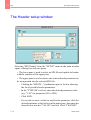
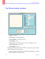
Download NOTE

User’s Manual
Vol. 1
CMXL V6.1
CM408 V6.0
0311401
January 2002
To contact SERCEL
Nantes, France
Commercial; Customer Support;
Manufacturing & Repair.
B.P. 439, 16 rue de Bel Air
44474 Carquefou Cedex
Tel: +33 2 40 30 11 81, Fax: +33 2 40 30 19 48
Hot-Line: Land:
+33 2 40 30 58 88
Marine: +33 2 40 30 59 59
E-mail: [email protected]
[email protected]
www.sercel.com
St Gaudens, France
Vibrator Customer Support;
Vibrator Manufacturing & Repair;
Streamer Manufacturing & Repair.
Tel: +33 5 61 89 90 00, Fax: +33 5 61 89 90 45
Hot Line: +33 5 61 89 90 91
Alfreton, U. K.
Streamer Manufacturing & Repair;
Customer Support.
Tel: +44 1 773 605 078, Fax: +44 1 773 541 778
Houston, USA
Commercial; Customer Support;
Manufacturing & Repair;
Streamer Manufacturing & Repair.
Tel: +1 281 492 66 88, Fax: +1 281 492 69 10
Hot-Line: +1 281 492 66 88
E-mail: [email protected]
[email protected]
[email protected]
Ponca City, USA
Vibrator Customer Support;
Vibrator Manufacturing & Repair.
Tel: +1 580 763 00 00, Fax: +1 580 763 00 22
Moscow, Russia
Commercial; Customer Support.
Tel: +7 095 254 06 59, Fax: +7 095 254 66 80
Beijing, P. R. of China
Commercial; Customer Support.
Tel: +86 106 43 76 661, Fax: +86 106 43 76 307
Tanggu, P. R. of China
Manufacturing & Repair.
Tel:+86 222 58 23 224 , Fax:+86 222 58 23 242
Xian, P. R. of China
Manufacturing & Repair.
Tel: +86 297 85 25 05, Fax: +86 297 85 55 04
Singapore
Streamer Manufacturing & Repair;
Customer Support.
Tel:+65 545 0411, Fax:+65 545 1418
Dehradun, India
Customer Support.
Tel: +91 135 773 387, Fax: +91 135 773 132
E-mail: [email protected]
In no event shall SERCEL be liable for incidental or consequential damages or related expenses
resulting from the use of this product, or arising out of or related to this manual or the information contained in it, even if SERCEL has been advised, or knew or should have known of the possibility of such damages.
The information included in this documentation is believed to be accurate and reliable.
However, SERCEL reserves the right to make changes to its products or specifications at any
time, without notice, in order to improve design or performance and to supply the best possible
product. This documentation does not form in any way a contractual agreement of sales promise
on the part of SERCEL.
Software mentioned in this documentation is sold under a precise licence agreement and as such
the documentation may cover technical areas for which the user may not have a final licence.
No part of this documentation, or any of the information included herein may be modified or
copied in any form or by any means without the prior written consent of SERCEL.
Acknowledgments: All brand or product names are trademarks or registered trademarks of their
respective companies or organizations.
408UL User’s Manual Vol.1
Table
of
Contents
1
Introduction
O v e r v i e w . . . .. . . .. . . .. . . .. . . .. . . .. . . .. . . .. . . .. . . .. . . .. . . .. . . .. . . .. . . .. 1- 2
T e r m i n o l o g y . . .. . . .. . . .. . . .. . . .. . . .. . . .. . . .. . . .. . . .. . . .. . . .. . . .. . . .. 1- 4
W o r k i n g wi t h w i n d o w s . . .. . . .. . . .. . . .. . . .. . . .. . . .. . . .. . . .. . . .. 1- 8
F i l e m e n u . . .. . . .. . . .. . . .. . . .. . . .. . . .. . . .. . . .. . . .. . . .. . . .. . . .. . . .. . . 1-13
General . . . . . . . . . . . . . . . . . . . . . . . . . . . . . . . . . . . . . . . . . . . . . . . 1-13
To save the setup parameters to a file. . . . . . . . . . . . . . . . . . . . . . . . 1-14
To restore the setup parameters from a file . . . . . . . . . . . . . . . . . . . 1-14
U t i l i t i e s .. . . .. . . .. . . .. . . .. . . .. . . .. . . .. . . .. . . .. . . .. . . .. . . .. . . .. . . .. . . 1-15
Snapshots . . . . . . . . . . . . . . . . . . . . . . . . . . . . . . . . . . . . . . . . . . . . . 1-15
Copy And Paste . . . . . . . . . . . . . . . . . . . . . . . . . . . . . . . . . . . . . . . . 1-16
Drag And Drop . . . . . . . . . . . . . . . . . . . . . . . . . . . . . . . . . . . . . . . . . 1-16
"HCI Print" utility . . . . . . . . . . . . . . . . . . . . . . . . . . . . . . . . . . . . . . . 1-17
How to select text . . . . . . . . . . . . . . . . . . . . . . . . . . . . . . . . . . . . . . . 1-17
Miscellaneous . . . . . . . . . . . . . . . . . . . . . . . . . . . . . . . . . . . . . . . . . . 1-18
2
408UL Install
T h e 4 0 8 UL I n s t a l l wi n d o w . .. . . .. . . .. . . .. . . .. . . .. . . .. . . .. . . .. 2- 2
Overview. . . . . . . . . . . . . . . . . . . . . . . . . . . . . . . . . . . . . . . . . . . . . . . 2-2
Configuration . . . . . . . . . . . . . . . . . . . . . . . . . . . . . . . . . . . . . . . . . . . 2-3
0311401
i
Table of Contents
408UL User’s Manual Vol.1
HCI . . . . . . . . . . . . . . . . . . . . . . . . . . . . . . . . . . . . . . . . . . . . . . . . . . . 2-8
I n s t a l l i n g P R M s o f t w a r e ( C MX L u s e r s ) . . .. . . .. . . .. . . 2-10
Overview. . . . . . . . . . . . . . . . . . . . . . . . . . . . . . . . . . . . . . . . . . . . . . 2-10
Installing PRM on the HCI workstation . . . . . . . . . . . . . . . . . . . . . . 2-11
Installing PRM on a remote station . . . . . . . . . . . . . . . . . . . . . . . . . 2-12
3
Configuration
T h e mai n w i n d o w . . .. . . .. . . .. . . .. . . .. . . .. . . .. . . .. . . .. . . .. . . .. . . .. 3- 2
Overview. . . . . . . . . . . . . . . . . . . . . . . . . . . . . . . . . . . . . . . . . . . . . . . 3-2
File menu . . . . . . . . . . . . . . . . . . . . . . . . . . . . . . . . . . . . . . . . . . . . . . 3-3
Status pane . . . . . . . . . . . . . . . . . . . . . . . . . . . . . . . . . . . . . . . . . . . . . 3-3
Customer Support icon . . . . . . . . . . . . . . . . . . . . . . . . . . . . . . . . . . . . 3-3
T h e Vi e w m e n u . . .. . . .. . . .. . . .. . . .. . . .. . . .. . . .. . . .. . . .. . . .. . . .. . . .. 3- 5
Overview. . . . . . . . . . . . . . . . . . . . . . . . . . . . . . . . . . . . . . . . . . . . . . . 3-5
UC Modules Configuration (CM408 users) . . . . . . . . . . . . . . . . . . . . 3-5
Software Configuration. . . . . . . . . . . . . . . . . . . . . . . . . . . . . . . . . . . . 3-6
Copyrights. . . . . . . . . . . . . . . . . . . . . . . . . . . . . . . . . . . . . . . . . . . . . . 3-6
Identity Card . . . . . . . . . . . . . . . . . . . . . . . . . . . . . . . . . . . . . . . . . . . . 3-7
Clear Status . . . . . . . . . . . . . . . . . . . . . . . . . . . . . . . . . . . . . . . . . . . . . 3-7
T h e S e t u p me n u . .. . . .. . . .. . . .. . . .. . . .. . . .. . . .. . . .. . . .. . . .. . . .. . . .. 3- 8
Crew setup window . . . . . . . . . . . . . . . . . . . . . . . . . . . . . . . . . . . . . . 3-8
User Info . . . . . . . . . . . . . . . . . . . . . . . . . . . . . . . . . . . . . . . . . . . . . . 3-10
UC Module Configuration (CM408 users). . . . . . . . . . . . . . . . . . . . 3-10
O n Li n e / O f f L i n e . . . .. . . .. . . .. . . .. . . .. . . .. . . .. . . .. . . .. . . .. . . .. . . 3-12
Overview. . . . . . . . . . . . . . . . . . . . . . . . . . . . . . . . . . . . . . . . . . . . . . 3-12
Wireline telemetry . . . . . . . . . . . . . . . . . . . . . . . . . . . . . . . . . . . . . . 3-13
Radio or dual telemetry. . . . . . . . . . . . . . . . . . . . . . . . . . . . . . . . . . . 3-14
ii
January 2002
408UL User’s Manual Vol.1
4
Table of Contents
Line
T h e mai n w i n d o w . . .. . . .. . . .. . . .. . . .. . . .. . . .. . . .. . . .. . . .. . . .. . . .. 4- 2
T o p o g r a p h i c v i e w . . .. . . .. . . .. . . .. . . .. . . .. . . .. . . .. . . .. . . .. . . .. . . .. 4- 5
General . . . . . . . . . . . . . . . . . . . . . . . . . . . . . . . . . . . . . . . . . . . . . . . . 4-5
Sensors view . . . . . . . . . . . . . . . . . . . . . . . . . . . . . . . . . . . . . . . . . . . . 4-7
Seismonitor . . . . . . . . . . . . . . . . . . . . . . . . . . . . . . . . . . . . . . . . . . . . . 4-8
Instruments view. . . . . . . . . . . . . . . . . . . . . . . . . . . . . . . . . . . . . . . . 4-10
Batteries view . . . . . . . . . . . . . . . . . . . . . . . . . . . . . . . . . . . . . . . . . . 4-11
Working with graphic views. . . . . . . . . . . . . . . . . . . . . . . . . . . . . . . 4-12
N u me r i c v i e w .. . . .. . . .. . . .. . . .. . . .. . . .. . . .. . . .. . . .. . . .. . . .. . . .. . . 4-18
H i s t o g r a m v i e w . .. . . .. . . .. . . .. . . .. . . .. . . .. . . .. . . .. . . .. . . .. . . .. . . 4-20
T h e S u r v e y s e t u p w i n d o w . . .. . . .. . . .. . . .. . . .. . . .. . . .. . . .. . . 4-21
General . . . . . . . . . . . . . . . . . . . . . . . . . . . . . . . . . . . . . . . . . . . . . . . 4-21
Survey . . . . . . . . . . . . . . . . . . . . . . . . . . . . . . . . . . . . . . . . . . . . . . . . 4-22
Point Code. . . . . . . . . . . . . . . . . . . . . . . . . . . . . . . . . . . . . . . . . . . . . 4-24
Sensor . . . . . . . . . . . . . . . . . . . . . . . . . . . . . . . . . . . . . . . . . . . . . . . . 4-26
T h e L a y o u t s e t u p w i n d o w . . .. . . .. . . .. . . .. . . .. . . .. . . .. . . .. . . 4-28
General . . . . . . . . . . . . . . . . . . . . . . . . . . . . . . . . . . . . . . . . . . . . . . . 4-28
Marker. . . . . . . . . . . . . . . . . . . . . . . . . . . . . . . . . . . . . . . . . . . . . . . . 4-29
Aux . . . . . . . . . . . . . . . . . . . . . . . . . . . . . . . . . . . . . . . . . . . . . . . . . . 4-33
Detour . . . . . . . . . . . . . . . . . . . . . . . . . . . . . . . . . . . . . . . . . . . . . . . . 4-35
Mute . . . . . . . . . . . . . . . . . . . . . . . . . . . . . . . . . . . . . . . . . . . . . . . . . 4-36
LRU . . . . . . . . . . . . . . . . . . . . . . . . . . . . . . . . . . . . . . . . . . . . . . . . . 4-37
REM . . . . . . . . . . . . . . . . . . . . . . . . . . . . . . . . . . . . . . . . . . . . . . . . . 4-37
SU6-R . . . . . . . . . . . . . . . . . . . . . . . . . . . . . . . . . . . . . . . . . . . . . . . . 4-37
T h e S p r e a d s s e t u p wi n d o w . .. . . .. . . .. . . .. . . .. . . .. . . .. . . .. . . 4-38
General . . . . . . . . . . . . . . . . . . . . . . . . . . . . . . . . . . . . . . . . . . . . . . . 4-38
Absolute spreads . . . . . . . . . . . . . . . . . . . . . . . . . . . . . . . . . . . . . . . . 4-39
Generic spreads. . . . . . . . . . . . . . . . . . . . . . . . . . . . . . . . . . . . . . . . . 4-41
T h e P r e f e r e n c e s s e t u p wi n d o w . . . .. . . .. . . .. . . .. . . .. . . .. . . 4-44
0311401
iii
Table of Contents
408UL User’s Manual Vol.1
General . . . . . . . . . . . . . . . . . . . . . . . . . . . . . . . . . . . . . . . . . . . . . . . 4-44
Graphic . . . . . . . . . . . . . . . . . . . . . . . . . . . . . . . . . . . . . . . . . . . . . . . 4-45
Cloning . . . . . . . . . . . . . . . . . . . . . . . . . . . . . . . . . . . . . . . . . . . . . . . 4-46
Histogram . . . . . . . . . . . . . . . . . . . . . . . . . . . . . . . . . . . . . . . . . . . . . 4-48
T h e L o o k P r o p e r t i e s S e t u p m e n u . . . .. . . .. . . .. . . .. . . .. . . 4-49
A d v a n c e d l a y o u t s . . .. . . .. . . .. . . .. . . .. . . .. . . .. . . .. . . .. . . .. . . .. . . 4-50
Detour with skipped receiver points . . . . . . . . . . . . . . . . . . . . . . . . . 4-50
Snaking layout . . . . . . . . . . . . . . . . . . . . . . . . . . . . . . . . . . . . . . . . . 4-51
Logical line mapped with several physical lines (CMXL only). . . . 4-52
Skipped channels . . . . . . . . . . . . . . . . . . . . . . . . . . . . . . . . . . . . . . . 4-54
W o r k i n g wi t h F D U 3 C u n i t s .. . . .. . . .. . . .. . . .. . . .. . . .. . . .. . . 4-56
General . . . . . . . . . . . . . . . . . . . . . . . . . . . . . . . . . . . . . . . . . . . . . . . 4-56
FDU3C in the Survey Setup . . . . . . . . . . . . . . . . . . . . . . . . . . . . . . . 4-58
FDU3C in the Layout Setup . . . . . . . . . . . . . . . . . . . . . . . . . . . . . . . 4-60
FDU3C in the Spread Setup . . . . . . . . . . . . . . . . . . . . . . . . . . . . . . . 4-60
FDU3C in the Test Setup . . . . . . . . . . . . . . . . . . . . . . . . . . . . . . . . . 4-60
W o r k i n g wi t h L R U s . . . .. . . .. . . .. . . .. . . .. . . .. . . .. . . .. . . .. . . .. . . 4-61
General . . . . . . . . . . . . . . . . . . . . . . . . . . . . . . . . . . . . . . . . . . . . . . . 4-61
LRU frequency management . . . . . . . . . . . . . . . . . . . . . . . . . . . . . . 4-63
Desensitization . . . . . . . . . . . . . . . . . . . . . . . . . . . . . . . . . . . . . . . . . 4-65
TDM (Time Division Multiplex) . . . . . . . . . . . . . . . . . . . . . . . . . . . 4-66
The LRU Layout Setup window. . . . . . . . . . . . . . . . . . . . . . . . . . . . 4-67
Normal parameters . . . . . . . . . . . . . . . . . . . . . . . . . . . . . . . . . . . . . . 4-68
Advanced parameters . . . . . . . . . . . . . . . . . . . . . . . . . . . . . . . . . . . . 4-69
Sleep . . . . . . . . . . . . . . . . . . . . . . . . . . . . . . . . . . . . . . . . . . . . . . . . . 4-72
Loop . . . . . . . . . . . . . . . . . . . . . . . . . . . . . . . . . . . . . . . . . . . . . . . . . 4-72
R a d i o o r Dua l t e l e me t r y .. . . .. . . .. . . .. . . .. . . .. . . .. . . .. . . .. . . 4-73
General . . . . . . . . . . . . . . . . . . . . . . . . . . . . . . . . . . . . . . . . . . . . . . . 4-73
Parameters. . . . . . . . . . . . . . . . . . . . . . . . . . . . . . . . . . . . . . . . . . . . . 4-74
Working with REMs. . . . . . . . . . . . . . . . . . . . . . . . . . . . . . . . . . . . . 4-78
How to change Transmit and Receive frequencies. . . . . . . . . . . . . . 4-80
iv
January 2002
408UL User’s Manual Vol.1
Table of Contents
Working with both REMs and LRUs . . . . . . . . . . . . . . . . . . . . . . . . 4-82
R a d i o s e c t i o n m a n a g e me n t . .. . . .. . . .. . . .. . . .. . . .. . . .. . . .. . . 4-84
General . . . . . . . . . . . . . . . . . . . . . . . . . . . . . . . . . . . . . . . . . . . . . . . 4-84
Parameters. . . . . . . . . . . . . . . . . . . . . . . . . . . . . . . . . . . . . . . . . . . . . 4-85
Working with SU6-Rs . . . . . . . . . . . . . . . . . . . . . . . . . . . . . . . . . . . 4-86
Quick Deploy . . . . . . . . . . . . . . . . . . . . . . . . . . . . . . . . . . . . . . . . . . 4-90
T e s t f u n c t i o n s . . . .. . . .. . . .. . . .. . . .. . . .. . . .. . . .. . . .. . . .. . . .. . . .. . . 4-91
Overview. . . . . . . . . . . . . . . . . . . . . . . . . . . . . . . . . . . . . . . . . . . . . . 4-91
Instrument tests . . . . . . . . . . . . . . . . . . . . . . . . . . . . . . . . . . . . . . . . . 4-93
Field tests . . . . . . . . . . . . . . . . . . . . . . . . . . . . . . . . . . . . . . . . . . . . . 4-95
Seismonitor . . . . . . . . . . . . . . . . . . . . . . . . . . . . . . . . . . . . . . . . . . . . 4-98
C h e c k Li n e .. . . .. . . .. . . .. . . .. . . .. . . .. . . .. . . .. . . .. . . .. . . .. . . .. . . .. . . 4-99
General . . . . . . . . . . . . . . . . . . . . . . . . . . . . . . . . . . . . . . . . . . . . . . . 4-99
Line Troubleshooting . . . . . . . . . . . . . . . . . . . . . . . . . . . . . . . . . . . 4-100
Network Management. . . . . . . . . . . . . . . . . . . . . . . . . . . . . . . . . . . 4-102
F T MU / F T S U Li n e d i s p a t c h i n g ( C MX L ) . . .. . . .. . . .. . 4-104
5
Operation
T h e Mai n W i n d o w . .. . . .. . . .. . . .. . . .. . . .. . . .. . . .. . . .. . . .. . . .. . . .. 5- 2
Overview. . . . . . . . . . . . . . . . . . . . . . . . . . . . . . . . . . . . . . . . . . . . . . . 5-2
File . . . . . . . . . . . . . . . . . . . . . . . . . . . . . . . . . . . . . . . . . . . . . . . . . . . 5-3
View . . . . . . . . . . . . . . . . . . . . . . . . . . . . . . . . . . . . . . . . . . . . . . . . . . 5-4
Options . . . . . . . . . . . . . . . . . . . . . . . . . . . . . . . . . . . . . . . . . . . . . . . . 5-5
Look Props . . . . . . . . . . . . . . . . . . . . . . . . . . . . . . . . . . . . . . . . . . . . . 5-5
Print. . . . . . . . . . . . . . . . . . . . . . . . . . . . . . . . . . . . . . . . . . . . . . . . . . . 5-5
Check . . . . . . . . . . . . . . . . . . . . . . . . . . . . . . . . . . . . . . . . . . . . . . . . . 5-6
T h e P r o c e s s Typ e S e t u p w i n d o w . .. . . .. . . .. . . .. . . .. . . .. . . .. 5- 7
Overview. . . . . . . . . . . . . . . . . . . . . . . . . . . . . . . . . . . . . . . . . . . . . . . 5-7
To Generate a Process Type . . . . . . . . . . . . . . . . . . . . . . . . . . . . . . . 5-8
Impulsive type. . . . . . . . . . . . . . . . . . . . . . . . . . . . . . . . . . . . . . . . . . 5-13
0311401
v
Table of Contents
408UL User’s Manual Vol.1
Impulsive Stack. . . . . . . . . . . . . . . . . . . . . . . . . . . . . . . . . . . . . . . . . 5-14
Correlation Before Stack . . . . . . . . . . . . . . . . . . . . . . . . . . . . . . . . . 5-16
Correlation After Stack. . . . . . . . . . . . . . . . . . . . . . . . . . . . . . . . . . . 5-19
Vibro Stack . . . . . . . . . . . . . . . . . . . . . . . . . . . . . . . . . . . . . . . . . . . . 5-20
T h e S i g n a l T y p e S e t u p w i n d o w . . . .. . . .. . . .. . . .. . . .. . . .. . . 5-22
Overview. . . . . . . . . . . . . . . . . . . . . . . . . . . . . . . . . . . . . . . . . . . . . . 5-22
Signal type options . . . . . . . . . . . . . . . . . . . . . . . . . . . . . . . . . . . . . . 5-23
To generate a Signal Type Setup . . . . . . . . . . . . . . . . . . . . . . . . . . . 5-24
More About Synthetic Signal Files. . . . . . . . . . . . . . . . . . . . . . . . . . 5-25
Similarity tests . . . . . . . . . . . . . . . . . . . . . . . . . . . . . . . . . . . . . . . . . 5-28
T h e Ope r a t io n S o u r c e S e t u p w i n d o w . . .. . . .. . . .. . . .. . . 5-29
Operation parameters . . . . . . . . . . . . . . . . . . . . . . . . . . . . . . . . . . . . 5-29
To generate a Source Operation Setup . . . . . . . . . . . . . . . . . . . . . . 5-33
T h e Ope r a t i o n S i g n a l S e t u p wi n d o w . . . .. . . .. . . .. . . .. . . 5-34
T h e Obs e r v e r ’ s Com m e n t T y p e S e t u p w i n d o w . .. . . 5-35
T h e S h o o t e r S e t u p w i n d o w . .. . . .. . . .. . . .. . . .. . . .. . . .. . . .. . . 5-36
Overview. . . . . . . . . . . . . . . . . . . . . . . . . . . . . . . . . . . . . . . . . . . . . . 5-36
To generate a Shooter Setup . . . . . . . . . . . . . . . . . . . . . . . . . . . . . . . 5-37
Dynamite/Airgun (RF Blaster only) . . . . . . . . . . . . . . . . . . . . . . . . . 5-38
Fire Blaster Timing pane (RF Blaster only) . . . . . . . . . . . . . . . . . . . 5-38
Cap Limits. . . . . . . . . . . . . . . . . . . . . . . . . . . . . . . . . . . . . . . . . . . . . 5-41
Uphole Geophone Continuity . . . . . . . . . . . . . . . . . . . . . . . . . . . . . . 5-41
Uphole Channel Description pane (RF Blaster only) . . . . . . . . . . . . 5-41
Shooter Setup pane (RF Blaster only) . . . . . . . . . . . . . . . . . . . . . . . 5-42
T h e Obs e r v e r R e p o r t S e t u p w i n d o w . . . .. . . .. . . .. . . .. . . 5-43
T h e S l i p T i m e S e t u p m e n u . .. . . .. . . .. . . .. . . .. . . .. . . .. . . .. . . 5-44
T o s t a r t , s t o p a n d e x e c u t e a s h o t .. . . .. . . .. . . .. . . .. . . .. . . 5-45
General . . . . . . . . . . . . . . . . . . . . . . . . . . . . . . . . . . . . . . . . . . . . . . . 5-45
GO. . . . . . . . . . . . . . . . . . . . . . . . . . . . . . . . . . . . . . . . . . . . . . . . . . . 5-48
STOP. . . . . . . . . . . . . . . . . . . . . . . . . . . . . . . . . . . . . . . . . . . . . . . . . 5-48
ABORT. . . . . . . . . . . . . . . . . . . . . . . . . . . . . . . . . . . . . . . . . . . . . . . 5-48
vi
January 2002
408UL User’s Manual Vol.1
Table of Contents
Automation . . . . . . . . . . . . . . . . . . . . . . . . . . . . . . . . . . . . . . . . . . . . 5-49
The Look Properties menu . . . . . . . . . . . . . . . . . . . . . . . . . . . . . . . . 5-52
Shot data retrieval . . . . . . . . . . . . . . . . . . . . . . . . . . . . . . . . . . . . . . . 5-53
T h e Re s u l t s p a n e . . . .. . . .. . . .. . . .. . . .. . . .. . . .. . . .. . . .. . . .. . . .. . . 5-55
S l i p - s w e e p .. . . .. . . .. . . .. . . .. . . .. . . .. . . .. . . .. . . .. . . .. . . .. . . .. . . .. . . 5-58
Theory of operation . . . . . . . . . . . . . . . . . . . . . . . . . . . . . . . . . . . . . 5-58
How to implement slip-sweep . . . . . . . . . . . . . . . . . . . . . . . . . . . . . 5-59
N a v i g a t i o n - d r i v e n s h o o t i n g .. . . .. . . .. . . .. . . .. . . .. . . .. . . .. . . 5-61
T B i n Rad i o o r D u a l t e l e m e t r y . . . .. . . .. . . .. . . .. . . .. . . .. . . 5-62
TB in Vibroseis Radio or Dual telemetry . . . . . . . . . . . . . . . . . . . . . 5-62
Adjusting the delay between F. O. and Firing (Explosive) . . . . . . . 5-63
S h o o t i n g w i t h a n L S S .. . . .. . . .. . . .. . . .. . . .. . . .. . . .. . . .. . . .. . . 5-65
Overview. . . . . . . . . . . . . . . . . . . . . . . . . . . . . . . . . . . . . . . . . . . . . . 5-65
Taking a shot with an LSI. . . . . . . . . . . . . . . . . . . . . . . . . . . . . . . . . 5-66
M o r e A b o u t C o r r e l a t i o n .. . . .. . . .. . . .. . . .. . . .. . . .. . . .. . . .. . . 5-69
Description . . . . . . . . . . . . . . . . . . . . . . . . . . . . . . . . . . . . . . . . . . . . 5-69
Data Distribution. . . . . . . . . . . . . . . . . . . . . . . . . . . . . . . . . . . . . . . . 5-72
6
Noise Editing
T h e mai n w i n d o w . . .. . . .. . . .. . . .. . . .. . . .. . . .. . . .. . . .. . . .. . . .. . . .. 6- 2
Overview. . . . . . . . . . . . . . . . . . . . . . . . . . . . . . . . . . . . . . . . . . . . . . . 6-2
Auto/Manual . . . . . . . . . . . . . . . . . . . . . . . . . . . . . . . . . . . . . . . . . . . . 6-3
Hold/Var . . . . . . . . . . . . . . . . . . . . . . . . . . . . . . . . . . . . . . . . . . . . . . . 6-3
Init Thresh. . . . . . . . . . . . . . . . . . . . . . . . . . . . . . . . . . . . . . . . . . . . . . 6-3
Load Thresh . . . . . . . . . . . . . . . . . . . . . . . . . . . . . . . . . . . . . . . . . . . . 6-3
Save Thresh. . . . . . . . . . . . . . . . . . . . . . . . . . . . . . . . . . . . . . . . . . . . . 6-3
T h e Noi s e Edi t i n g S e t u p wi n d o w .. . . .. . . .. . . .. . . .. . . .. . . .. 6- 5
M o r e A b o u t N o i s e E l i m i n a t i o n . . . .. . . .. . . .. . . .. . . .. . . .. . . .. 6- 9
"Spike Editing" method . . . . . . . . . . . . . . . . . . . . . . . . . . . . . . . . . . . 6-9
Diversity Stack . . . . . . . . . . . . . . . . . . . . . . . . . . . . . . . . . . . . . . . . . 6-12
0311401
vii
Table of Contents
408UL User’s Manual Vol.1
T h e Re s u l t s p a n e . . . .. . . .. . . .. . . .. . . .. . . .. . . .. . . .. . . .. . . .. . . .. . . 6-16
7
Recorder
T h e mai n w i n d o w . . .. . . .. . . .. . . .. . . .. . . .. . . .. . . .. . . .. . . .. . . .. . . .. 7- 2
Overview. . . . . . . . . . . . . . . . . . . . . . . . . . . . . . . . . . . . . . . . . . . . . . . 7-2
File . . . . . . . . . . . . . . . . . . . . . . . . . . . . . . . . . . . . . . . . . . . . . . . . . . . 7-2
T h e T a p e S e t u p w i n d o w . .. . . .. . . .. . . .. . . .. . . .. . . .. . . .. . . .. . . .. 7- 3
The Tape Transport Configurati on s e tup window . 7-5
A u t o / M a n u a l . .. . . .. . . .. . . .. . . .. . . .. . . .. . . .. . . .. . . .. . . .. . . .. . . .. . . .. 7- 7
General . . . . . . . . . . . . . . . . . . . . . . . . . . . . . . . . . . . . . . . . . . . . . . . . 7-7
AUTO Mode . . . . . . . . . . . . . . . . . . . . . . . . . . . . . . . . . . . . . . . . . . . . 7-8
MANUAL MODE . . . . . . . . . . . . . . . . . . . . . . . . . . . . . . . . . . . . . . . 7-9
F u n c t i o n B u t t o n s . . . .. . . .. . . .. . . .. . . .. . . .. . . .. . . .. . . .. . . .. . . .. . . 7-11
R e s u l t s . .. . . .. . . .. . . .. . . .. . . .. . . .. . . .. . . .. . . .. . . .. . . .. . . .. . . .. . . .. . . 7-16
8
Plotter (CM408 users)
T h e mai n w i n d o w . . .. . . .. . . .. . . .. . . .. . . .. . . .. . . .. . . .. . . .. . . .. . . .. 8- 2
Overview. . . . . . . . . . . . . . . . . . . . . . . . . . . . . . . . . . . . . . . . . . . . . . . 8-2
File . . . . . . . . . . . . . . . . . . . . . . . . . . . . . . . . . . . . . . . . . . . . . . . . . . . 8-3
T h e Opt i o n me n u . . . .. . . .. . . .. . . .. . . .. . . .. . . .. . . .. . . .. . . .. . . .. . . .. 8- 4
AUTO option . . . . . . . . . . . . . . . . . . . . . . . . . . . . . . . . . . . . . . . . . . . 8-4
MANUAL option . . . . . . . . . . . . . . . . . . . . . . . . . . . . . . . . . . . . . . . . 8-5
T h e AG C S E TU P p a n e . . . .. . . .. . . .. . . .. . . .. . . .. . . .. . . .. . . .. . . .. 8- 6
General . . . . . . . . . . . . . . . . . . . . . . . . . . . . . . . . . . . . . . . . . . . . . . . . 8-6
AGC Off . . . . . . . . . . . . . . . . . . . . . . . . . . . . . . . . . . . . . . . . . . . . . . . 8-7
AGC On . . . . . . . . . . . . . . . . . . . . . . . . . . . . . . . . . . . . . . . . . . . . . . . 8-8
Sample normalization for a camera . . . . . . . . . . . . . . . . . . . . . . . . . 8-10
T h e CA M E RA p a n e . . . .. . . .. . . .. . . .. . . .. . . .. . . .. . . .. . . .. . . .. . . 8-12
T h e P LO T S E L EC T I O N p a n e . .. . . .. . . .. . . .. . . .. . . .. . . .. . . 8-14
T h e AG C On P r o p e r t i e s s e t u p w i n d o w .. . . .. . . .. . . .. . . 8-16
viii
January 2002
408UL User’s Manual Vol.1
Table of Contents
T h e P l o t Gr o u p T y p e s e t u p w i n d o w .. . . .. . . .. . . .. . . .. . . 8-18
Plot Group Type parameters . . . . . . . . . . . . . . . . . . . . . . . . . . . . . . . 8-18
To generate a Plot Group Type setup . . . . . . . . . . . . . . . . . . . . . . . . 8-20
9
Plotter (CMXL users)
T h e mai n w i n d o w . . .. . . .. . . .. . . .. . . .. . . .. . . .. . . .. . . .. . . .. . . .. . . .. 9- 2
Overview. . . . . . . . . . . . . . . . . . . . . . . . . . . . . . . . . . . . . . . . . . . . . . . 9-2
Enabled/Disabled . . . . . . . . . . . . . . . . . . . . . . . . . . . . . . . . . . . . . . . . 9-4
Plot Again . . . . . . . . . . . . . . . . . . . . . . . . . . . . . . . . . . . . . . . . . . . . . . 9-4
Abort Plot . . . . . . . . . . . . . . . . . . . . . . . . . . . . . . . . . . . . . . . . . . . . . . 9-4
File . . . . . . . . . . . . . . . . . . . . . . . . . . . . . . . . . . . . . . . . . . . . . . . . . . . 9-4
S e l e c t i n g t r a c e s t o b e p l o t t e d . .. . . .. . . .. . . .. . . .. . . .. . . .. . . .. 9- 5
T h e P r o c e s s i n g p a r a me t e r s .. . . .. . . .. . . .. . . .. . . .. . . .. . . .. . . .. 9- 7
General . . . . . . . . . . . . . . . . . . . . . . . . . . . . . . . . . . . . . . . . . . . . . . . . 9-7
Control . . . . . . . . . . . . . . . . . . . . . . . . . . . . . . . . . . . . . . . . . . . . . . . . 9-7
Scaling . . . . . . . . . . . . . . . . . . . . . . . . . . . . . . . . . . . . . . . . . . . . . . . . 9-9
Filters . . . . . . . . . . . . . . . . . . . . . . . . . . . . . . . . . . . . . . . . . . . . . . . . 9-10
T h e P l o t p a r a me t e r s . . .. . . .. . . .. . . .. . . .. . . .. . . .. . . .. . . .. . . .. . .
F i e l d t e s t s . .. . . .. . . .. . . .. . . .. . . .. . . .. . . .. . . .. . . .. . . .. . . .. . . .. . . .. . .
I n s t r u m e n t t e s t s .. . . .. . . .. . . .. . . .. . . .. . . .. . . .. . . .. . . .. . . .. . . .. . .
T h e S i n g l e T r a c e d i s p l a y . . . .. . . .. . . .. . . .. . . .. . . .. . . .. . . .. . .
9-12
9-15
9-16
9-17
Overview. . . . . . . . . . . . . . . . . . . . . . . . . . . . . . . . . . . . . . . . . . . . . . 9-17
Processing parameters. . . . . . . . . . . . . . . . . . . . . . . . . . . . . . . . . . . . 9-18
Plot parameters . . . . . . . . . . . . . . . . . . . . . . . . . . . . . . . . . . . . . . . . . 9-18
Annotation parameters . . . . . . . . . . . . . . . . . . . . . . . . . . . . . . . . . . . 9-18
10 Positioning
T h e mai n w i n d o w . . .. . . .. . . .. . . .. . . .. . . .. . . .. . . .. . . .. . . .. . . .. . . 10-2
Overview. . . . . . . . . . . . . . . . . . . . . . . . . . . . . . . . . . . . . . . . . . . . . . 10-2
How to use the Zoom function . . . . . . . . . . . . . . . . . . . . . . . . . . . . . 10-3
0311401
ix
Table of Contents
408UL User’s Manual Vol.1
Manual scale . . . . . . . . . . . . . . . . . . . . . . . . . . . . . . . . . . . . . . . . . . . 10-4
How to load a graphic file to the hard disk. . . . . . . . . . . . . . . . . . . . 10-5
G r a p h i c d i s p l a y o f t h e s p r e a d .. . . .. . . .. . . .. . . .. . . .. . . .. . . 10-6
Overview. . . . . . . . . . . . . . . . . . . . . . . . . . . . . . . . . . . . . . . . . . . . . . 10-6
How to use the Positioning main window . . . . . . . . . . . . . . . . . . . . 10-6
How to interpret the graphic view . . . . . . . . . . . . . . . . . . . . . . . . . . 10-7
Source Attributes . . . . . . . . . . . . . . . . . . . . . . . . . . . . . . . . . . . . . . 10-11
More about the estimated COG position . . . . . . . . . . . . . . . . . . . . 10-12
Launching a shot from the Positioning main window . . . . . . . . . . 10-13
T h e Dat u m T y p e s e t u p wi n d o w . . . .. . . .. . . .. . . .. . . .. . . .. . 10-15
T h e P r o j e c t i o n T y p e s e t u p w i n d o w . .. . . .. . . .. . . .. . . .. . 10-17
T h e Vi e w s e t u p w i n d o w . .. . . .. . . .. . . .. . . .. . . .. . . .. . . .. . . .. . 10-19
T h e I ma g e s e t u p w i n d o w .. . . .. . . .. . . .. . . .. . . .. . . .. . . .. . . .. . 10-20
T h e Mar k e r s e t u p w i n d o w . .. . . .. . . .. . . .. . . .. . . .. . . .. . . .. . 10-24
T h e Qua l i t y War n i n g s e t u p w i n d o w .. . . .. . . .. . . .. . . .. . 10-26
V e h i c l e t r a c k i n g .. . . .. . . .. . . .. . . .. . . .. . . .. . . .. . . .. . . .. . . .. . . .. . 10-28
Overview. . . . . . . . . . . . . . . . . . . . . . . . . . . . . . . . . . . . . . . . . . . . . 10-28
Supported vehicle tracking systems . . . . . . . . . . . . . . . . . . . . . . . . 10-31
Alert scheme . . . . . . . . . . . . . . . . . . . . . . . . . . . . . . . . . . . . . . . . . . 10-33
Requesting a vehicle to move . . . . . . . . . . . . . . . . . . . . . . . . . . . . . 10-35
Playing back a vehicle's trackline . . . . . . . . . . . . . . . . . . . . . . . . . . 10-36
Sending a message to a vehicle. . . . . . . . . . . . . . . . . . . . . . . . . . . . 10-36
T h e Ve h i c l e L o g s e t u p w i n d o w . . . .. . . .. . . .. . . .. . . .. . . .. . 10-37
T h e B a s e s e t u p w i n d o w . . .. . . .. . . .. . . .. . . .. . . .. . . .. . . .. . . .. . 10-41
Overview. . . . . . . . . . . . . . . . . . . . . . . . . . . . . . . . . . . . . . . . . . . . . 10-41
To place a base station icon into your survey map view . . . . . . . . 10-42
To move the base station icon within the survey map view . . . . . . 10-42
To delete the base station icon . . . . . . . . . . . . . . . . . . . . . . . . . . . . 10-42
T h e Wat c h d o g s e t u p w i n d o w . . .. . . .. . . .. . . .. . . .. . . .. . . .. . 10-43
T h e Me s s a g e s e t u p w i n d o w .. . . .. . . .. . . .. . . .. . . .. . . .. . . .. . 10-46
T h e Ve h i c l e I d e n t i t y s e t u p w i n d o w . .. . . .. . . .. . . .. . . .. . 10-48
x
January 2002
408UL User’s Manual Vol.1
Table of Contents
B a s i c G e o d e s y Gl o s s a r y . .. . . .. . . .. . . .. . . .. . . .. . . .. . . .. . . .. . 10-51
11 Log
T h e mai n w i n d o w . . .. . . .. . . .. . . .. . . .. . . .. . . .. . . .. . . .. . . .. . . .. . . 11-2
Overview. . . . . . . . . . . . . . . . . . . . . . . . . . . . . . . . . . . . . . . . . . . . . . 11-2
Data Transfer . . . . . . . . . . . . . . . . . . . . . . . . . . . . . . . . . . . . . . . . . . 11-3
Text editor. . . . . . . . . . . . . . . . . . . . . . . . . . . . . . . . . . . . . . . . . . . . . 11-5
Drag and Drop . . . . . . . . . . . . . . . . . . . . . . . . . . . . . . . . . . . . . . . . . 11-5
T h e Dat a b a s e L i s t s e t u p wi n d o w .. . . .. . . .. . . .. . . .. . . .. . . 11-6
Overview. . . . . . . . . . . . . . . . . . . . . . . . . . . . . . . . . . . . . . . . . . . . . . 11-6
To generate a Data Base View list . . . . . . . . . . . . . . . . . . . . . . . . . . 11-7
T h e P a g e S e t t i n g Typ e s e t u p w i n d o w . . .. . . .. . . .. . . .. . . 11-8
Overview. . . . . . . . . . . . . . . . . . . . . . . . . . . . . . . . . . . . . . . . . . . . . . 11-8
To generate a Pagination Type . . . . . . . . . . . . . . . . . . . . . . . . . . . . . 11-9
Glossary of parameters . . . . . . . . . . . . . . . . . . . . . . . . . . . . . . . . . . 11-11
The
The
The
Log
S h o o t i n g s e t u p w i n d o w .. . . .. . . .. . . .. . . .. . . .. . . .. . . .. . 11-16
T e x t L i s t s e t u p wi n d o w . . . .. . . .. . . .. . . .. . . .. . . .. . . .. . 11-19
Voi d F i l e s e t u p wi n d o w . . . .. . . .. . . .. . . .. . . .. . . .. . . .. . 11-23
Vi e w . . .. . . .. . . .. . . .. . . .. . . .. . . .. . . .. . . .. . . .. . . .. . . .. . . .. . . .. . 11-24
Overview. . . . . . . . . . . . . . . . . . . . . . . . . . . . . . . . . . . . . . . . . . . . . 11-24
Exporting an Observer Report . . . . . . . . . . . . . . . . . . . . . . . . . . . . 11-25
Exporting DPG Status Data . . . . . . . . . . . . . . . . . . . . . . . . . . . . . . 11-26
Exporting source COG results . . . . . . . . . . . . . . . . . . . . . . . . . . . . 11-28
Exporting receiver position history data . . . . . . . . . . . . . . . . . . . . 11-29
D a t a B a s e V i e w . .. . . .. . . .. . . .. . . .. . . .. . . .. . . .. . . .. . . .. . . .. . . .. . 11-31
Overview. . . . . . . . . . . . . . . . . . . . . . . . . . . . . . . . . . . . . . . . . . . . . 11-31
Exporting operating parameters or results . . . . . . . . . . . . . . . . . . . 11-33
Exporting a description of the system configuration . . . . . . . . . . . 11-34
M e d i a Vi e w . . . .. . . .. . . .. . . .. . . .. . . .. . . .. . . .. . . .. . . .. . . .. . . .. . . .. . 11-35
Overview. . . . . . . . . . . . . . . . . . . . . . . . . . . . . . . . . . . . . . . . . . . . . 11-35
0311401
xi
Table of Contents
408UL User’s Manual Vol.1
Importing 408UL script files . . . . . . . . . . . . . . . . . . . . . . . . . . . . . 11-36
Importing SPS files. . . . . . . . . . . . . . . . . . . . . . . . . . . . . . . . . . . . . 11-37
Floppy disk utility. . . . . . . . . . . . . . . . . . . . . . . . . . . . . . . . . . . . . . 11-38
4 0 8 U L S e t u p s c r i p t f o r ma t . .. . . .. . . .. . . .. . . .. . . .. . . .. . . .. . 11-39
12 VE432
T h e mai n w i n d o w . . .. . . .. . . .. . . .. . . .. . . .. . . .. . . .. . . .. . . .. . . .. . . 12-2
Overview. . . . . . . . . . . . . . . . . . . . . . . . . . . . . . . . . . . . . . . . . . . . . . 12-2
File . . . . . . . . . . . . . . . . . . . . . . . . . . . . . . . . . . . . . . . . . . . . . . . . . . 12-3
View . . . . . . . . . . . . . . . . . . . . . . . . . . . . . . . . . . . . . . . . . . . . . . . . . 12-3
Check . . . . . . . . . . . . . . . . . . . . . . . . . . . . . . . . . . . . . . . . . . . . . . . . 12-5
Reconfiguration . . . . . . . . . . . . . . . . . . . . . . . . . . . . . . . . . . . . . . . . 12-5
T h e Vi b r a t o r Cr e w S e t u p wi n d o w . . .. . . .. . . .. . . .. . . .. . . 12-7
Crew setup parameters . . . . . . . . . . . . . . . . . . . . . . . . . . . . . . . . . . . 12-7
To generate a Crew Setup. . . . . . . . . . . . . . . . . . . . . . . . . . . . . . . . . 12-9
T h e B a s i c T y p e S e t u p w i n d o w .. . . .. . . .. . . .. . . .. . . .. . . .. . 12-10
Overview. . . . . . . . . . . . . . . . . . . . . . . . . . . . . . . . . . . . . . . . . . . . . 12-10
Linear . . . . . . . . . . . . . . . . . . . . . . . . . . . . . . . . . . . . . . . . . . . . . . . 12-12
LOG . . . . . . . . . . . . . . . . . . . . . . . . . . . . . . . . . . . . . . . . . . . . . . . . 12-14
Tn . . . . . . . . . . . . . . . . . . . . . . . . . . . . . . . . . . . . . . . . . . . . . . . . . . 12-15
Pulse . . . . . . . . . . . . . . . . . . . . . . . . . . . . . . . . . . . . . . . . . . . . . . . . 12-16
Pseudorandom. . . . . . . . . . . . . . . . . . . . . . . . . . . . . . . . . . . . . . . . . 12-17
Custom . . . . . . . . . . . . . . . . . . . . . . . . . . . . . . . . . . . . . . . . . . . . . . 12-19
Compound. . . . . . . . . . . . . . . . . . . . . . . . . . . . . . . . . . . . . . . . . . . . 12-21
Delay. . . . . . . . . . . . . . . . . . . . . . . . . . . . . . . . . . . . . . . . . . . . . . . . 12-22
Deboost option . . . . . . . . . . . . . . . . . . . . . . . . . . . . . . . . . . . . . . . . 12-22
How to generate a Basic Type . . . . . . . . . . . . . . . . . . . . . . . . . . . . 12-23
T h e Ac q u i s i t i o n T y p e S e t u p wi n d o w . . . .. . . .. . . .. . . .. . 12-24
T h e Rad i o M a n a g e m e n t S e t u p w i n d o w .. . . .. . . .. . . .. . 12-28
T h e QC L i m i t s S e t u p w i n d o w . .. . . .. . . .. . . .. . . .. . . .. . . .. . 12-31
xii
January 2002
408UL User’s Manual Vol.1
Table of Contents
T h e QC C h o i c e s e t u p wi n d o w . .. . . .. . . .. . . .. . . .. . . .. . . .. . 12-32
T h e T 0 S e t u p w i n d o w .. . . .. . . .. . . .. . . .. . . .. . . .. . . .. . . .. . . .. . 12-33
T h e f u n c t i o n b u t t o n s . .. . . .. . . .. . . .. . . .. . . .. . . .. . . .. . . .. . . .. . 12-35
Auto/Manual . . . . . . . . . . . . . . . . . . . . . . . . . . . . . . . . . . . . . . . . . . 12-35
Look . . . . . . . . . . . . . . . . . . . . . . . . . . . . . . . . . . . . . . . . . . . . . . . . 12-36
Vib Fleet . . . . . . . . . . . . . . . . . . . . . . . . . . . . . . . . . . . . . . . . . . . . . 12-38
Local Acq . . . . . . . . . . . . . . . . . . . . . . . . . . . . . . . . . . . . . . . . . . . . 12-40
Set DSD . . . . . . . . . . . . . . . . . . . . . . . . . . . . . . . . . . . . . . . . . . . . . 12-42
Get DSD . . . . . . . . . . . . . . . . . . . . . . . . . . . . . . . . . . . . . . . . . . . . . 12-44
Get QC . . . . . . . . . . . . . . . . . . . . . . . . . . . . . . . . . . . . . . . . . . . . . . 12-47
Radio Delay . . . . . . . . . . . . . . . . . . . . . . . . . . . . . . . . . . . . . . . . . . 12-54
Set Servo . . . . . . . . . . . . . . . . . . . . . . . . . . . . . . . . . . . . . . . . . . . . . 12-59
Statistics . . . . . . . . . . . . . . . . . . . . . . . . . . . . . . . . . . . . . . . . . . . . . 12-62
N o r ma l a c q u i s i t i o n .. . . .. . . .. . . .. . . .. . . .. . . .. . . .. . . .. . . .. . . .. . 12-66
General . . . . . . . . . . . . . . . . . . . . . . . . . . . . . . . . . . . . . . . . . . . . . . 12-66
Graphic view. . . . . . . . . . . . . . . . . . . . . . . . . . . . . . . . . . . . . . . . . . 12-68
Numeric view . . . . . . . . . . . . . . . . . . . . . . . . . . . . . . . . . . . . . . . . . 12-70
DPG/DSD status codes . . . . . . . . . . . . . . . . . . . . . . . . . . . . . . . . . . 12-72
V S R . . .. . . .. . . .. . . .. . . .. . . .. . . .. . . .. . . .. . . .. . . .. . . .. . . .. . . .. . . .. . . .. . 12-73
Overview. . . . . . . . . . . . . . . . . . . . . . . . . . . . . . . . . . . . . . . . . . . . . 12-73
Example . . . . . . . . . . . . . . . . . . . . . . . . . . . . . . . . . . . . . . . . . . . . . 12-73
13 SPS
T h e mai n w i n d o w . . .. . . .. . . .. . . .. . . .. . . .. . . .. . . .. . . .. . . .. . . .. . . 13-2
Overview. . . . . . . . . . . . . . . . . . . . . . . . . . . . . . . . . . . . . . . . . . . . . . 13-2
Device option button. . . . . . . . . . . . . . . . . . . . . . . . . . . . . . . . . . . . . 13-3
Database . . . . . . . . . . . . . . . . . . . . . . . . . . . . . . . . . . . . . . . . . . . . . . 13-4
T h e T e x t s e t u p w i n d o w . . .. . . .. . . .. . . .. . . .. . . .. . . .. . . .. . . .. . . 13-5
T h e He a d e r s e t u p w i n d o w . . .. . . .. . . .. . . .. . . .. . . .. . . .. . . .. . . 13-6
T h e Re c o r d s e t u p w i n d o w . . .. . . .. . . .. . . .. . . .. . . .. . . .. . . .. . . 13-8
0311401
xiii
Table of Contents
408UL User’s Manual Vol.1
T h e Voi d f i l e s e t u p w i n d o w .. . . .. . . .. . . .. . . .. . . .. . . .. . . .. . 13-10
S P S Vi e w . . .. . . .. . . .. . . .. . . .. . . .. . . .. . . .. . . .. . . .. . . .. . . .. . . .. . . .. . 13-11
M e d i a Vi e w . . . .. . . .. . . .. . . .. . . .. . . .. . . .. . . .. . . .. . . .. . . .. . . .. . . .. . 13-12
4 0 8 U L S c r i p t s Vi e w . . . .. . . .. . . .. . . .. . . .. . . .. . . .. . . .. . . .. . . .. . 13-13
W o r k i n g wi t h S P S f i l e s . . .. . . .. . . .. . . .. . . .. . . .. . . .. . . .. . . .. . 13-16
Creating SPS files from Observer Reports . . . . . . . . . . . . . . . . . . . 13-16
Creating or modifying SPS files . . . . . . . . . . . . . . . . . . . . . . . . . . . 13-17
Creating 408UL setup scripts from SPS files . . . . . . . . . . . . . . . . . 13-19
Merging 408UL SPS files in SPS coordinates files . . . . . . . . . . . . 13-21
14 VQC
O v e r v i e w . . . .. . . .. . . .. . . .. . . .. . . .. . . .. . . .. . . .. . . .. . . .. . . .. . . .. . . .. . . 14-2
T h e mai n w i n d o w . . .. . . .. . . .. . . .. . . .. . . .. . . .. . . .. . . .. . . .. . . .. . . 14-5
T h e I n s t a l l m e n u ( C MX L u s e r s o n l y ) . . .. . . .. . . .. . . .. . . 14-6
Connection parameters . . . . . . . . . . . . . . . . . . . . . . . . . . . . . . . . . . . 14-6
Licence . . . . . . . . . . . . . . . . . . . . . . . . . . . . . . . . . . . . . . . . . . . . . . . 14-7
T h e F i l e me n u . . . .. . . .. . . .. . . .. . . .. . . .. . . .. . . .. . . .. . . .. . . .. . . .. . . 14-8
Load/Save . . . . . . . . . . . . . . . . . . . . . . . . . . . . . . . . . . . . . . . . . . . . . 14-8
Copy . . . . . . . . . . . . . . . . . . . . . . . . . . . . . . . . . . . . . . . . . . . . . . . . . 14-9
T h e I mp o r t m e n u . . . .. . . .. . . .. . . .. . . .. . . .. . . .. . . .. . . .. . . .. . . .. . 14-11
T h e Vi e w m e n u . . .. . . .. . . .. . . .. . . .. . . .. . . .. . . .. . . .. . . .. . . .. . . .. . 14-13
Data Files . . . . . . . . . . . . . . . . . . . . . . . . . . . . . . . . . . . . . . . . . . . . 14-13
Clear Graphics . . . . . . . . . . . . . . . . . . . . . . . . . . . . . . . . . . . . . . . . 14-14
T h e S i g n a l T y p e S e t u p w i n d o w s . .. . . .. . . .. . . .. . . .. . . .. . 14-15
Overview. . . . . . . . . . . . . . . . . . . . . . . . . . . . . . . . . . . . . . . . . . . . . 14-15
Signal From 408UL Logic processor . . . . . . . . . . . . . . . . . . . . . . . 14-17
Signal From File . . . . . . . . . . . . . . . . . . . . . . . . . . . . . . . . . . . . . . . 14-18
T h e Cor r e l a t i o n T y p e S e t u p w i n d o w . . .. . . .. . . .. . . .. . 14-20
T h e S e q u e n c e T y p e S e t u p w i n d o w . . .. . . .. . . .. . . .. . . .. . 14-22
Overview. . . . . . . . . . . . . . . . . . . . . . . . . . . . . . . . . . . . . . . . . . . . . 14-22
xiv
January 2002
408UL User’s Manual Vol.1
Table of Contents
TRIGGER BY ACQ option . . . . . . . . . . . . . . . . . . . . . . . . . . . . . . 14-23
Amplitude/Time . . . . . . . . . . . . . . . . . . . . . . . . . . . . . . . . . . . . . . . 14-25
Frequency/Time . . . . . . . . . . . . . . . . . . . . . . . . . . . . . . . . . . . . . . . 14-27
Spectrum . . . . . . . . . . . . . . . . . . . . . . . . . . . . . . . . . . . . . . . . . . . . . 14-28
Phase & Distortion . . . . . . . . . . . . . . . . . . . . . . . . . . . . . . . . . . . . . 14-29
Harmonic Distortion . . . . . . . . . . . . . . . . . . . . . . . . . . . . . . . . . . . . 14-31
FT Analysis. . . . . . . . . . . . . . . . . . . . . . . . . . . . . . . . . . . . . . . . . . . 14-32
W o r k i n g wi t h V Q C .. . . .. . . .. . . .. . . .. . . .. . . .. . . .. . . .. . . .. . . .. . 14-33
Overview. . . . . . . . . . . . . . . . . . . . . . . . . . . . . . . . . . . . . . . . . . . . . 14-33
Real-time analysis. . . . . . . . . . . . . . . . . . . . . . . . . . . . . . . . . . . . . . 14-33
Post-processing . . . . . . . . . . . . . . . . . . . . . . . . . . . . . . . . . . . . . . . . 14-34
W o r k i n g wi t h g r a p h s . .. . . .. . . .. . . .. . . .. . . .. . . .. . . .. . . .. . . .. . 14-36
Overview. . . . . . . . . . . . . . . . . . . . . . . . . . . . . . . . . . . . . . . . . . . . . 14-36
2D graph . . . . . . . . . . . . . . . . . . . . . . . . . . . . . . . . . . . . . . . . . . . . . 14-38
3D graph . . . . . . . . . . . . . . . . . . . . . . . . . . . . . . . . . . . . . . . . . . . . 14-39
T h e Gr a p h P r o p e r t i e s m e n u . . . .. . . .. . . .. . . .. . . .. . . .. . . .. . 14-40
U n i t C o n v e r s i o n .. . . .. . . .. . . .. . . .. . . .. . . .. . . .. . . .. . . .. . . .. . . .. . 14-42
Signal unit . . . . . . . . . . . . . . . . . . . . . . . . . . . . . . . . . . . . . . . . . . . 14-42
International System units . . . . . . . . . . . . . . . . . . . . . . . . . . . . . . . 14-43
15 VE416
T h e mai n w i n d o w . . .. . . .. . . .. . . .. . . .. . . .. . . .. . . .. . . .. . . .. . . .. . . 15-2
Overview. . . . . . . . . . . . . . . . . . . . . . . . . . . . . . . . . . . . . . . . . . . . . . 15-2
File . . . . . . . . . . . . . . . . . . . . . . . . . . . . . . . . . . . . . . . . . . . . . . . . . . 15-3
View . . . . . . . . . . . . . . . . . . . . . . . . . . . . . . . . . . . . . . . . . . . . . . . . . 15-3
Check . . . . . . . . . . . . . . . . . . . . . . . . . . . . . . . . . . . . . . . . . . . . . . . . 15-4
T h e B a s i c T y p e s e t u p w i n d o w .. . . .. . . .. . . .. . . .. . . .. . . .. . . 15-5
Overview. . . . . . . . . . . . . . . . . . . . . . . . . . . . . . . . . . . . . . . . . . . . . . 15-5
Sinewave-type signals. . . . . . . . . . . . . . . . . . . . . . . . . . . . . . . . . . . . 15-8
Pulse type . . . . . . . . . . . . . . . . . . . . . . . . . . . . . . . . . . . . . . . . . . . . 15-12
0311401
xv
Table of Contents
408UL User’s Manual Vol.1
Pseudorandom. . . . . . . . . . . . . . . . . . . . . . . . . . . . . . . . . . . . . . . . . 15-13
How to generate a basic type . . . . . . . . . . . . . . . . . . . . . . . . . . . . . 15-14
T h e S we e p T y p e s e t u p w i n d o w . . . .. . . .. . . .. . . .. . . .. . . .. . 15-16
Sweep Type setup parameters. . . . . . . . . . . . . . . . . . . . . . . . . . . . . 15-16
How to generate a sweep type . . . . . . . . . . . . . . . . . . . . . . . . . . . . 15-17
T h e Ac q u i s i t i o n T y p e s e t u p w i n d o w . . . .. . . .. . . .. . . .. . 15-18
Acquisition Type setup parameters. . . . . . . . . . . . . . . . . . . . . . . . . 15-18
How to generate an Acquisition Type Setup . . . . . . . . . . . . . . . . . 15-21
The
The
The
The
The
The
Re t u r n S i g n a l s s e t u p wi n d o w . . . .. . . .. . . .. . . .. . . .. . 15-22
QC L i m i t s s e t u p w i n d o w . .. . . .. . . .. . . .. . . .. . . .. . . .. . 15-24
Rad i o s e t u p w i n d o w .. . . .. . . .. . . .. . . .. . . .. . . .. . . .. . . .. . 15-26
DSD L i m i t s s e t u p w i n d o w .. . . .. . . .. . . .. . . .. . . .. . . .. . 15-29
I n v a l i d S w e e p s e t u p wi n d o w .. . . .. . . .. . . .. . . .. . . .. . 15-30
f u n c t i o n b u t t o n s . .. . . .. . . .. . . .. . . .. . . .. . . .. . . .. . . .. . . .. . 15-31
Auto/Manual . . . . . . . . . . . . . . . . . . . . . . . . . . . . . . . . . . . . . . . . . . 15-31
Look . . . . . . . . . . . . . . . . . . . . . . . . . . . . . . . . . . . . . . . . . . . . . . . . 15-31
Radio delay . . . . . . . . . . . . . . . . . . . . . . . . . . . . . . . . . . . . . . . . . . . 15-34
Set Servo . . . . . . . . . . . . . . . . . . . . . . . . . . . . . . . . . . . . . . . . . . . . . 15-36
Get DSD . . . . . . . . . . . . . . . . . . . . . . . . . . . . . . . . . . . . . . . . . . . . . 15-39
Set DSD . . . . . . . . . . . . . . . . . . . . . . . . . . . . . . . . . . . . . . . . . . . . . 15-43
Local Acquisition . . . . . . . . . . . . . . . . . . . . . . . . . . . . . . . . . . . . . . 15-45
Get QC . . . . . . . . . . . . . . . . . . . . . . . . . . . . . . . . . . . . . . . . . . . . . . 15-49
Normal Acquisition. . . . . . . . . . . . . . . . . . . . . . . . . . . . . . . . . . . . . 15-52
N o r ma l A c q u i s i t i o n r e s u l t s .. . . .. . . .. . . .. . . .. . . .. . . .. . . .. . 15-54
Overview. . . . . . . . . . . . . . . . . . . . . . . . . . . . . . . . . . . . . . . . . . . . . 15-54
Example with four acquisitions and three DSDs . . . . . . . . . . . . . . 15-54
With the Real-Time button activated. . . . . . . . . . . . . . . . . . . . . . . 15-57
With the Statistics button activated . . . . . . . . . . . . . . . . . . . . . . . . 15-58
M o r e a b o u t t h e r a d i o d e l a y .. . . .. . . .. . . .. . . .. . . .. . . .. . . .. . 15-61
The radio delay . . . . . . . . . . . . . . . . . . . . . . . . . . . . . . . . . . . . . . . . 15-61
Radio delay measurement. . . . . . . . . . . . . . . . . . . . . . . . . . . . . . . . 15-62
xvi
January 2002
408UL User’s Manual Vol.1
Table of Contents
D P G/ DSD s t a t u s c o d e s . . . .. . . .. . . .. . . .. . . .. . . .. . . .. . . .. . . .. . 15-65
16 RF spectrum
T h e mai n w i n d o w . . .. . . .. . . .. . . .. . . .. . . .. . . .. . . .. . . .. . . .. . . .. . . 16-2
Overview. . . . . . . . . . . . . . . . . . . . . . . . . . . . . . . . . . . . . . . . . . . . . . 16-2
File . . . . . . . . . . . . . . . . . . . . . . . . . . . . . . . . . . . . . . . . . . . . . . . . . . 16-2
Window. . . . . . . . . . . . . . . . . . . . . . . . . . . . . . . . . . . . . . . . . . . . . . . 16-3
T h e S e t u p me n u . .. . . .. . . .. . . .. . . .. . . .. . . .. . . .. . . .. . . .. . . .. . . .. . . 16-4
RF spectrum setup parameters . . . . . . . . . . . . . . . . . . . . . . . . . . . . . 16-4
RF Spectrum Monitoring view . . . . . . . . . . . . . . . . . . . . . . . . . . . . . 16-6
T h e RF S p e c t r u m Mon i t o r i n g f u n c t i o n . . . .. . . .. . . .. . . 16-8
Theory of operation . . . . . . . . . . . . . . . . . . . . . . . . . . . . . . . . . . . . . 16-8
General Index
0311401
xvii
Table of Contents
xviii
408UL User’s Manual Vol.1
January 2002
Chapter
1
408UL User’s Manual
Volume 1
Introduction
This chapter includes the following sections:
• Overview (page 1-2)
• Terminology (page 1-4)
• Working with windows (page 1-8)
• File menu (page 1-13)
• Utilities (page 1-15)
0311401
1-1
1
Introduction
Overview
Overview
This manual provides operating instructions for the 408UL system’s
Graphic User Interface (referred to as HCI).
Before using this manual, you need to install the system by following
the instructions given in the 408UL Installation Manual.
The User’s Manual is automatically loaded from the 408UL CDROM
to your workstation’s disk as you load the 408UL software package.
Then it is just one click away at all times, using the HELP button
available in every main window, or it can be viewed using the menu that
pops up when you press the mouse centre button. With a PC computer
equipped with a PDF file reader (Adobe Acrobat Reader) you can view
this manual direct from the 408UL CDROM’s DOC directory.
This manual assumes you are familiar with window-driven systems and
you know how to work with windows, including how to use a mouse
and standard menus and commands, and to open, move, resize, shrink,
restore and close a window. For help with any of these techniques, see
the documentation that came with your workstation.
408UL documentation consists of the following manuals:
• Installation Manual (0311400): contains an introduction to the
408UL system, installation information, a few instructions for the
operator to get started, and reference information that will help you
select a 408UL configuration tailored to your needs.
• User’s Manual Volume 1 (0311401): this manual.
• User’s Manual Volume 2 (0311402): contains information on
interfaces (description of Input/Output formats, including SEGD
format).
• User’s Manual Volume 3 (0311403): contains reference
information on the definition of parameters involved in the HCI or in
the instrumentation.
1-2
January 2002
User’s Manual Vol. 1
Overview
• Technical Manual (0311404): contains maintenance information
and associated procedures and diagrams, including LT408 and
TMS408 documentation.
0311401
1-3
1
1
Introduction
Terminology
Terminology
You’ll need to be familiar with a number of terms that are described
below.
• Click
To press and release a mouse button quickly (left-hand button, unless
otherwise specified).
• Command button
A button that carries out a command (Add, Change, Delete, Swap,
Reverse) with the parameters specified in the text boxes.
• Dialog box
A secondary window that provides or requests information within an
environment's main window.
• Double-click
To press and release the left-hand mouse button twice in rapid
succession without moving the mouse.
• Drag
To move an item on the screen by holding down the mouse button while
moving the mouse. See Drag And Drop (page 1-16).
• Icon
A small graphical image used to represent a window. Windows can be
turned into icons or minimized to save room or unclutter the workspace.
1-4
January 2002
User’s Manual Vol. 1
Terminology
1
Option button
Index box
Text box
Pushbutton
List box
Scrollbar
Scale box
Toggle buttons
(shown
activated)
• Index box
A text box (usually the first box from left to right) showing the
identification number of a row (or set of rows) to be generated in a list
box or selected from a list box.
• List box
A box used to display a scrollable list of the rows edited under a text
box.
0311401
1-5
1
Introduction
Terminology
• Mouse buttons
With the mouse pointer resting on any 408UL window, always use the
LEFT-HAND button, unless otherwise (very exceptionally) specified.
With the mouse pointer resting anywhere in the workspace (outside any
window) :
- the LEFT-HAND button is used to select the Root menu, refresh
the screen, quit the Motif window manager (Mwm) or restart
Mwm.
- the CENTRE button is used to call utility programs (e.g. File
Manager, Snapshot, etc.) See "SNAPSHOT" below for
instructions to get a hardcopy of a window.
- the RIGHT-HAND button is used to start 408UL environments
(i.e. open 408UL main windows). The menu which pops up
allows you to access any main window (whether closed, or
shrunk to an icon or hidden) at any time.
• Option button
A pushbutton used to post an option menu in which you can select an
option. An option button displays the label of the selected option and a
bar graphic to distinguish it from a command button.
• Point (to)
To move the mouse pointer on the screen until it rests on the item you
want to select.
• Scale
A rectangular box, with a slider in it, used to set or display a value in a
range. A label indicates the current value. A value is selected by
dragging the slider and releasing the mouse button when the desired
value is displayed. Clicking on either side of the slider selects the next
higher or lower value.
1-6
January 2002
User’s Manual Vol. 1
Terminology
• Scrollbar
A rectangular box, with a slider and direction arrow graphics in it, used
to scroll the visible area of a window pane or box. The slider indicates
the relative position and size of the visible area. The position is adjusted
by dragging the slider or clicking the direction arrows.
• Select
To point to an item in a menu, by dragging the mouse pointer until the
item is highlighted, and release the mouse button.
• Text box
An entry box used to enter or display values and/or text for a parameter
within a dialog box.
• Toggle button
A pushbutton composed of a label preceded by a graphic (diamond or
square) with two distinctive states that indicate the set and unset states
of the button.
There are two special cases of toggle buttons.
• Radio button: used to select one option from a number of options.
Each option is represented by a radio button. Each button represents
a mutually exclusive selection (only one radio button can be set at a
time).
• Check button: used to set a number of options. Unlike a
radiobutton, any number of check buttons can be set at the same time.
0311401
1-7
1
1
Introduction
Working with windows
Working with windows
• Conventions
The following conventions are used in the description below:
m, n, o, p: stand for sequential numbers
i
: stands for an increment (positive or negative); the + sign is
optional
v
: stands for any allowable value for a parameter.
All other symbols are part of the syntax.
• General rules
• Clicking in a text box causes the text cursor (I-beam pointer) to
appear in it, allowing you to type the desired information. To make
corrections, use the BACKSPACE or DEL key as applicable.
• The CARRIAGE RETURN key is only used to enter two or more
text lines into the same text box,
• In any dialog box, the allowable values for each text box will
automatically show up if you click ADD (or APPLY if there is no
ADD button) whenever the text box is blank
• Double-clicking in a text box causes its content to be highlighted.
Then, pressing any key erases the content and enters the
corresponding character.
• Clicking on any row in a list box selects the row (its number shows
up in the index box). See the example below.
• Double-clicking on any row in a list box selects the row and causes
the content of the row to show up in the text boxes. See the example
below.
1-8
January 2002
User’s Manual Vol. 1
Working with windows
1
Example: In the list box that follows
:
Double-click "2"
Click "3"
Click CHANGE
1
2
3
11
21
31
12
22
32
Index box
Text box 1
Text box 2
2
3
3
21
21
31
22
22
32
• In an index box:
m-n
selects all rows from row m to row n.
m-
selects all rows from row m to the end of the list.
-m
selects all rows from the beginning of the list to row m.
-
selects the whole list.
m-n/i
selects rows m, m+i, m+2i, m+3i...n
n-m/-i
selects rows n, n-i, n-2i, m-3i...m
• In a text box:
/
means the current value in the list box will not be changed.
V
means the value V will be applied to the specified row or set
of rows.
V/i
or V/+i (or V/-i) means an incremental (or decremental) value
starting from V will be applied to the specified set of rows.
(The + sign is optional).
/i
or /+i (or /-i) means an increment (or decrement) will be
applied to the pre-existing values of the specified set of rows.
0311401
1-9
1
Introduction
Working with windows
• ADD button
Used to generate a row or a set of rows, unless it is already defined in
the list box. The rows to be created are specified in the index box as
shown in the examples below :
1
generates row 1 in the list box.
1-5
generates rows 1, 2, 3, 4, 5
1-8/2
generates rows 1, 3, 5, 7
7-2/-2
generates rows 7, 5, 3
• CHANGE button
Used to update a row or a set of rows (already defined in the list box)
with the contents of one or more text boxes. The rows to be updated are
specified in the index box as shown in the examples below:
1
updates row 1
1-5
updates rows 1 through 5
5-
updates all rows from No. 5 to the end of the list
-5
updates all rows from the first sequential number in the list to
No. 5.
-
updates the whole list.
Assuming the list box contains rows 10, 20, 8, 11, 12, 15, 30 (starting
with 10 and ending with 30):
-/2
updates rows 10, 8, 12, 30
10-15/2 updates rows 10, 8, 12
1-10
20-/2
updates rows 20, 11, 15
-15/2
updates rows 10, 8, 12
January 2002
User’s Manual Vol. 1
Working with windows
• DELETE button
Used to delete a row or set of rows defined in the list box and specified
in the index box as shown in the examples below:
1
deletes row 1
1-5
deletes row 1 through 5
5-
deletes all rows from No. 5 to the end of the list
-5
deletes all rows from the first sequential number in the list to
No. 5
-
deletes the whole list.
• REVERSE button
Used to reverse the order of a set of a rows specified in the index box as
shown in the examples below:
0311401
Index box
List box
Before clicking
REVERSE
List box
After clicking
REVERSES
1-5
12345
54321
3-
12345
12543
-3
12345
32145
-
12345
54321
1-11
1
1
Introduction
Working with windows
• SWAP button
Used to swap two sets of rows defined in the list box and specified in
the index box. The two sets should not overlap. See the examples
below:
5-,7
Index box
List box
Before clicking
SWAP
List box
Before clicking
SWAP
5,7(or 7,5)
1 2 3 4 5 6 7 8 9 10
1 2 3 4 7 6 5 8 9 10
5,7-
1 2 3 4 5 6 7 8 9 10
1 2 3 4 7 8 9 10 6 5
5,7-9
1 2 3 4 5 6 7 8 9 10
1 2 3 4 7 8 9 6 5 10
-5,7
1 2 3 4 5 6 7 8 9 10
7 6 1 2 3 4 5 8 9 10
-5,7-
1 2 3 4 5 6 7 8 9 10
7 8 9 10 6 1 2 3 4 5
-5,7-9
1 2 3 4 5 6 7 8 9 10
7 8 9 6 1 2 3 4 5 10
3-5,7
1 2 3 4 5 6 7 8 9 10
1 2 7 6 3 4 5 8 9 10
3-5,7-
1 2 3 4 5 6 7 8 9 10
1 2 7 8 9 10 6 3 4 5
3-5,7-9
1 2 3 4 5 6 7 8 9 10
1 2 7 8 9 6 3 4 5 10
9, -5
1 2 3 4 5 6 7 8 9 10
9 6 7 8 1 2 3 4 5 10
9-, 5-7
1 2 3 4 5 6 7 8 9 10
1 2 3 4 9 10 8 5 6 7
9-, -5
1 2 3 4 5 6 7 8 9 10
9 10 6 7 8 1 2 3 4 5
7-9, -5
1 2 3 4 5 6 7 8 9 10
7 8 9 6 1 2 3 4 5 10
9-, 5
1 2 3 4 5 6 7 8 9 10
1 2 3 4 9 10 6 7 8 5
These two sets cannot be swapped because they overlap.
• APPLY button
Saves and/or activates the selections made in a main window or a dialog
box. If you wish to generate a file containing the parameters currently
displayed, use the “Load/Save” function in the “File” menu.
• RESET button
Restores the latest values saved in the list box when the APPLY button
was last used.
1-12
January 2002
User’s Manual Vol. 1
File menu
File menu
1
In this section:
• General (page 1-13)
• To save the setup parameters to a file (page 1-14)
• To restore the setup parameters from a file (page 1-14)
General
You can save the complete set of parameters you define in a main
window to a file, provided that you actually click the APPLY button
after setting the parameters in each secondary window. Subsequently,
you can restore the complete set of parameters from the file or delete the
complete file.
In the Configuration main window, the Load/Save command lets you
load or save (or delete) all parameters of all main windows in just one
click. Although relating to all main windows, the parameter files loaded
or saved in the Configuration main window are distinct from those
individually loaded or saved in the other main windows.
In any other main window, the Load/Save command loads or saves (or
deletes) only the parameters of the main window from which you select
the command.
Warning: After installing a new software release, do not load any
parameters from files saved with earlier releases.
0311401
1-13
1
Introduction
File menu
To save the setup parameters to a file
Click the “File...” menu in the Menu bar and select “Load/Save” from
the pull-down menu that pops up. This opens the Load/Save window:
type a name (16 ASCII characters max.) for the file to be saved, then
click the SAVE button and confirm your choice in the Warning box that
shows up. As a result, a file is created containing the complete set of
parameters currently used. After a while, the file name appears in the
list box, denoting the end of the Save operation. The list box may
contain up to 10 files.
To restore the setup parameters from a file
Click the "File..." menu in the Menu bar and select "Load/Save" from
the pull-down menu. In the dialog box that shows up, select (click) the
desired file name from the list box. As a result, the name is highlighted.
The name is also duplicated in the "Label" box above.
Click the LOAD button and confirm your choice in the Warning box
that shows up. After a while, the file name in the list box is deselected,
denoting the end of the Load operation. The complete set of parameters
contained in this file can now be used in this main window.
To activate the parameters loaded, after using the File LOAD command
from the Configuration (GO) main window, with On Line activated, but
the system being idle, you should click APPLY in the following
windows :
- CREW SETUP in Configuration main window,
- SURVEY SETUP window in LINE main window,
- PLOTTER main window.
In Radio or Dual configuration, if new RF parameters differ from the
current ones, it is necessary to make the appropriate changes in the RF
COMMUNICATION window.
1-14
January 2002
User’s Manual Vol. 1
Utilities
Utilities
1
In this section:
• Snapshots (page 1-15)
• Copy And Paste (page 1-16)
• Drag And Drop (page 1-16)
• "HCI Print" utility (page 1-17)
• How to select text (page 1-17)
• Miscellaneous (page 1-18)
Snapshots
With a graphic printer (e.g. HP5xx, or CANON BJC 4000, BJC70)
connected on the Parallel Printer port of the HCI workstation, you can
get hardcopies of any window as follows:
• With the centre button of the mouse, select SNAPSHOT or Invert
Black to White (outside any window).
• The mouse pointer should change to a sighting pointer (+).
• Click in the window you wish to print (with the left-hand button).
As a result the window is printed out.
Unless a graphic printer is used, selecting SNAPSHOT will open
MOTIF's standard snapshot dialog box.
Snapshots may be helpful when bargraphs or histograms are displayed
in the “Results” pane (e. g. VE432 main window).
NOTE: Use the "Invert Black to White" command rather than the direct
Snapshot command if you wish to swap black and white on the printout.
0311401
1-15
1
Introduction
Utilities
Copy And Paste
The Copy and Paste function allows you to copy data from a dialog box
to another. The procedure is as follows.
• With the mouse left button, select the data to be copied:
• If the data is in a text box:
- Point to the first character to be copied.
- Press the mouse left button and hold it down
- Move the mouse pointer to the last character to be copied
- Release the mouse button (the selected text is highlighted).
• If the data is in a graphic pane:
- Point to the upper-left corner of the area to be copied
- Press the mouse left button and hold it down
- Move the mouse pointer to the lower-right corner of the area to
be copied.
- Release the mouse button (the selected area is framed).
• Press the COPY key on the keyboard
• Click in the destination text box
• Press the PASTE key. As a result the selected data is inserted into
the text box.
Drag And Drop
The Drag and Drop function allows you to copy data from a Result pane
(text or graphics) or from a status pane direct to an application, via a
window pane or button.
The procedure is as follows :
• Click in the pane containing the data to be copied. If results are in
graphic form, select the desired area.
1-16
January 2002
User’s Manual Vol. 1
Utilities
• Press both the CONTROL key on the keyboard and the centre
button of the mouse, and hold them down (Press CONTROL first).
• Move the mouse to the desired window pane or button (i.e. "drag"
the selection) then click with the mouse left button (i.e. "drop" the
selection).
"HCI Print" utility
The HCI Print utility allows you to print all numerical values displayed
in a Results pane or Status pane. The procedure is as follows :
• With the centre button of the mouse, open the HCI print utility
window.
• With the mouse left button, click in the pane containing the data to
be printed out.
• Drag and drop (see above) the pane into the box in the HCI Print
window. As a result the data is printed out.
How to select text
• With the mouse left button, click the first character to be copied,
• Press the SHIFT key and hold it down,
• With the mouse left button, click the last character to be copied,
• Release the SHIFT key (the selected text is highlighted).
Alternately, if all of the text to be selected is viewed, you may:
• Point to the first character to be copied,
• Press the mouse left button and hold it down,
• Move the mouse pointer to the last character to be copied,
• Release the mouse button (the selected text is highlighted)
0311401
1-17
1
1
Introduction
Utilities
Miscellaneous
• When you close a main window, its position is saved, as well as the
position of each setup secondary window. When you open a window,
it appears where it was when the main window was last closed.
• If you activate the Num Lock key, you can type numerals with the
numeric key pad. In that case, with the current version of MOTIF, the
window control buttons (Minimize, Maximize, etc.) do not work.
1-18
January 2002
Chapter
2
408UL User’s Manual
Volume 1
408UL Install
This chapter describes the Installation window.
This chapter includes the following section:
• The 408UL Install window. See page 2-2
• Installing PRM software (CMXL users). See
page 2-10
0311401
2-1
2
408UL Install
The 408UL Install window
The 408UL Install window
In this section:
• Overview (page 2-2)
• Configuration (page 2-3)
• HCI (page 2-8)
Overview
Selecting “408UL Install” with the centre button of the mouse (outside
any window) opens a window to be used when you install the system or
whenever you install a new software version, or another type of
workstation (Master/Tx emulation) or vibrator electronics, or if you
change the number of screens or the “Save Screen” options, etc.
The look of the “ Install” window is not the same for CM408 and 408XL
control modules, but most parameters are the same. For a 408XL, see
also Installing PRM software (CMXL users) on page 2-10.
After making the desired selections in the “HCI Install” window, click
“APPLY”.
WARNING
The new settings will not take effect until you quit the window manager
(Quit Mwm) then restart the system.
In addition, after adding or changing an LCI board in a 408XL, the
system may ask you to reload LCI software (see 408UL Installation
manual).
2-2
January 2002
User’s Manual Vol. 1
The 408UL Install window
Configuration
.
2
CM408 users
CMXL users
• Telemetry type
The Lab type (CM408) or Telemetry type (408XL) buttons are used to
choose the type of telemetry.
• Cable: Choose this option if no radio telemetry units (REM, SU6R) are used. LRU radio relays and MWL micro-wave links can be
used, however.
• Radio: Choose this option if radio-only telemetry is contemplated.
The remote station units (SU6-R) can be used in wire-link mode,
however.
• Dual: Choose this option if a combination of wireline and radio
telemetry sections is contemplated.
0311401
2-3
2
408UL Install
The 408UL Install window
• Vibrator type
• VE432: to be selected if a VE432 from SERCEL is connected.
• VE416: to be selected if a VE416 from SERCEL is connected.
• VE416 Standalone: to be selected if an acquisition system other
than an 408UL is connected.
In cases where a VE416 is attached to an acquisition system other
than the 408UL, the HCI software can still be used to control the
DPG:
The DPG main window is used to operate the DPG in Remote
Control mode (Mode 240).
In the OPERATION main window, you generate an operation table
(list of shot points). To execute any shot point, you simply click it
in the operation table. This initializes the DPG. After the HCI has
received the Time Break from the DPG, you see the progress of the
acquisition sequences in the OPERATION main window, and
status messages from the VE416 are available in the DPG main
window (where they can be displayed, analyzed, etc.).
• Other: to be selected if any other type of vibrator electronics is
connected.
• Plotter type
• 12 inch plotter.
• 24 inch plotter.
NOTE for CM408 users: With the GS612 type, the "Trace Sequential"
option in the Plot Group Type setup of the PLOTTER environment is
not available.
NOTE for CMXL users: Enter a name for each plotter in the
associated “Name” text box. The name will appear in the Plotter main
window to identify each plotter.
2-4
January 2002
User’s Manual Vol. 1
The 408UL Install window
• Number of plotters (CMXL only)
Choose the appropriate option (1 or 2) depending on the number of
plotters attached to the system.
2
• Blaster type
• SHOT PRO (PELTON)
• OPSEIS 815
• SHALLOW
• OTHER (MACHA, etc.)
NOTE: If you select the “Work with LSI” option:
- the indicator LED on FDUs, otherwise used as a test result
indicator, is used to tell the shooter whether he is allowed to
connect/disconnect an LSI between two links.
- you cannot launch a new shot until retrieval of the previous one
is complete, whatever the field equipment and the shooting
method used.
• Printer Type
After you select the type of printer with this option button, clicking
APPLY will automatically install the appropriate spooler. The
following printers are supported :
• CANON
BJC4000, 4100 (parallel link, graphic).
BJC70 (parallel link, graphic).
• HP
5xx, 842C, 870Cxi (parallel link, graphic).
Thinkjet (serial link, text).
0311401
2-5
2
408UL Install
The 408UL Install window
• KODAK
Diconix 180SI (serial link, text).
• EPSON
Stylus Color 740, 760 (parallel link, graphic).
NOTE: The serial printer should be connected to serial port B.
• Mobile Receiver Unit (MRU)
If an MRU unit is connected to the station (i.e. if you wish to implement
the vehicle tracking function), select YES from the left-hand option
button. As a result you have to:
• select the port connected to the MRU (you are not allowed to select
termA if a VE416 DPG is installed),
• specify whether the tracklines of the vehicles should be recorded or
not, with the Log option button. If you select "ON" the trackline of
each vehicle will automatically be recorded to daily trackline files.
• Licences
These text boxes are used to enter the necessary passwords to enable the
software packages you wish to use.
CM408 users
2-6
CMXL users
January 2002
User’s Manual Vol. 1
The 408UL Install window
• LMP: 408UL control modules (CM408 or 408XL) come with
passwords recorded in the workstation prior to shipment and supplied
to you together with the accompanying documents. Each password is
computed from the serial number of each LMP board you purchased
(there may be up to five LMPs in a 408XL). The password of each
LMP to be used should be entered in one of the “LMP boards” text
boxes in this window. Unless the correct password is entered for each
LMP, you will not be allowed to activate GO in the OPERATION
main window.
If you have any difficulty recovering the password for an LMP board,
you can get it again from SERCEL: you simply have to supply the
Serial Number appearing on the printed circuit of the board.
• MRU: Likewise, if an MRU is used, you have to enter its password
(or else communications with the MRU will not be allowed).
• VQC: For CM408 users, the licence for the VQC application is
entered in this window. For CMXL users, it is entered in the VQC
main window.
• Plotter (CMXL users only): The licence for plotters cannot be
typed on the keyboard. It is supplied to you on a floppy disk.
To install the plotter licence, click on the License... button.
- A warning box should appear that asks you if you wish to install
a licence. If you choose to do that and a licence already exists,
you are going to overwrite that licence. The system prompts you
to insert the floppy disk containing the licence to install.
- Insert the floppy disk and click OK. This installs the plot licence.
- Wait for a warning box to appear, prompting you to remove the
floppy disk from the drive.
- Remove the floppy disk from the drive.
0311401
2-7
2
2
408UL Install
The 408UL Install window
WARNING
For CMXL users: After changing a plotter licence or installing a patch
on the HCI, you have to re-install PRM software if a remote PRM
station is used. See Installing PRM on a remote station on page 2-12
and choose the “Only PRM Application” option rather than “Solaris
and PRM Application”.
HCI
CM408 users
CMXL users
• Master
To be selected if the screen is attached to the workstation on which the
HCI software is running.
• Tx emulation
To be selected if the screen is attached to a workstation used as Xterminal.
2-8
January 2002
User’s Manual Vol. 1
The 408UL Install window
• Nb of screens
Number of screens attached to the workstation. If you select "2", you are
required to specify the side (Left/Right) on which the extension screen
is located, so that the mouse pointer can jump to the suitable border
from one screen to the other when moved horizontally.
• Screen Saver
Clicking the "Properties" button opens a dialog box used to assign a
name (e.g. an operator's name) to the workspace configuration saved by
the SAVE SCREEN command accessible with the mouse right button
(outside any window).
The names, if any, contained in the list box are prompted as options
whenever you select SAVE SCREEN or RESTART with the mouse
right button.
If, prior to shutting down the workstation, you select SAVE SCREEN
with a given name, then the main windows that were open when you
saved the screen will automatically be opened at the same place when
you restart the system (by selecting RESTART) with the same name.
SAVE SCREEN also saves the positions of the secondary windows (but
not the state).
To enter a new name (e.g. your name) type it in the "Name" text box,
then click ADD. As a result the new name shows up in the list box
(unless it already exists). The "Change" and "Del" (Delete) buttons
allow you to make any changes needed to the list of names.
0311401
2-9
2
2
408UL Install
Installing PRM software (CMXL users)
Installing PRM software (CMXL users)
In this section:
• Overview (page 2-10)
• Installing PRM on the HCI workstation (page 2-11)
• Installing PRM on a remote station (page 2-12)
Overview
PRM software controls the formatting of the data to a tape drive, a
plotter and SQC-Pro. You can install PRM software on the HCI or a
separate station.
In the “408XL Install” window, click on the PRM tab.
IMPORTANT
Installation of Solaris and Sercel software on the HCI is assumed
completed.
2-10
January 2002
User’s Manual Vol. 1
Installing PRM software (CMXL users)
2
Installing PRM on the HCI workstation
To install PRM software on the HCI workstation, simply choose the
Local option in the 408XL Install window. (Also choose the Number
of LCI/LMP boards).
Click Apply. Wait for installation to be complete (about 1/4 hour, i. e.
until the cursor in the HCI console window stops spinning).
After installation of PRM is complete, you have to select “Quit Mwm”
and restart the station.
0311401
2-11
2
408UL Install
Installing PRM software (CMXL users)
Installing PRM on a remote station
To install Solaris on the remote PRM station, it is absolutely necessary
to use the “408XL Install” window. The CD-ROM drive of the remote
PRM station, if any is fitted, should not be used to install Solaris.
PREQUISITES:
• The plotter licence must be installed on the HCI prior to installing
PRM software on the remote station (so that the installation program
can copy the licence to the PRM station).
• Serial port A or B of the HCI workstation must be connected to
Serial port A of the remote station. Both stations must be connected
to the Ethernet network too.
• Power up both the HCI and the PRM station.
• In the HCI console window, type xlStopAppli <Return>.
In the 408XL Install window on the HCI, click on the PRM tab and do
the following:
• Control
• Type: Choose Remote.
• Number of LCI/LMP boards: Choose the total number of LCI
and LMP boards used (a 408XL unit can be equipped with up to five
LCI/LMP pairs).
• Installation
• Choose the software packages you wish to install, either Solaris
and PRM (e. g. on a first-time startup) or Only PRM (e. g. after
changing a plotter licence code or installing a patch on the HCI).
• Choose the Type of station on which to install PRM (Blade 1000).
• Choose the Serial Port of the HCI that is attached to the PRM
workstation. Serial port A or B of the HCI workstation must be
connected to Serial port A of the remote station. Be sure the remote
2-12
January 2002
User’s Manual Vol. 1
Installing PRM software (CMXL users)
station is connected to the HCI and started up. (Both stations must be
connected to the Ethernet network too).
After selecting the desired options, click on Apply then Install PRM
buttons and follow the instructions prompted on the display screen of
the HCI.
NOTE: If you are installing Solaris too, the system asks you to insert
the Solaris CD-ROM. Be sure the label on the CD-ROM reads
“SOLARIS 8 SOFTWARE 1 of 2”. Insert it into the CD-ROM drive
of the HCI.
Wait for installation to be complete (until the cursor in the HCI console
window stops spinning). Unless a problem arises (because of
connections, etc.) this should take less than a quarter of an hour if you
are installing only PRM software, and about an hour if you are installing
both Solaris and PRM.
After installation is complete, select “Quit Mwm” and restart the
workstation.
To restart a PRM station, power it off. Wait about 5 seconds. Power it
back on.
WARNING
After installation of PRM software on a remote station is complete,
disconnect the serial link from the two stations.
0311401
2-13
2
2
408UL Install
2-14
Installing PRM software (CMXL users)
January 2002
Chapter
3
408UL User’s Manual
Volume 1
Configuration
This chapter describes the Configuration environment
This chapter includes the following sections:
• The main window (page 3-2)
• The View menu (page 3-5)
• The Setup menu (page 3-8)
• On Line/Off Line (page 3-12)
0311401
3-1
3
Configuration
The main window
The main window
In this section:
• Overview (page 3-2)
• File menu (page 3-3)
• Status pane (page 3-3)
• Customer Support icon (page 3-3)
Overview
This window serves two main purposes:
• Firstly, it is used to set up some basic parameters at the beginning
of a survey, for instance the sample rate.
• Secondly, it is used to control and initiate communications with the
Central Unit each time the system is switched on.
3-2
January 2002
User’s Manual Vol. 1
The main window
An additional task is to report on the current hardware and software
configuration of the system, via the Identity Card.
File menu
Like all of the other environments, this main window has a Load/Save
option (explained in Chapter 1). However, in this window the function
is slightly different, since the file created contains all of the parameter
selections from ALL of the environments. In other words, File Load/
Save here has a global effect.
Warning: After installing a new software release, do not load any
parameters from files saved with earlier releases.
Status pane
If an arrow appears after the time in the "Status" pane, you can view
more information by double-clicking on the status.
In Multi-module configuration, if the status originates from an
acquisition module, the module number appears after the time, within
square brackets, along with the name of the board involved.
Customer Support icon
.
Clicking the telephone icon in the 408UL main
window opens a box providing information on how
to call the Customer Support Department for help.
Please note SERCEL Customer Support Hot Line with our dedicated
phone number:
0311401
- Outside FRANCE
+33 2 40 30 58 88
- In FRANCE
02 40 30 58 88
3-3
3
3
Configuration
The main window
This allows you to get in touch with our SERCEL Customer Support
Department, at any time and seven days a week, to ask any question
related to the use of your SERCEL equipment.
One of our experienced, english speaking Customer Support Engineers
will make every effort to give you any technical support you need.
The Hot Line includes a vocal mail box for calls outside normal
business hours: just leave a spoken message and we will get back to you
first thing in the morning (including Saturdays and Sundays).
SERCEL is committed to offering you our closest support for the
success of your field operations.
3-4
January 2002
User’s Manual Vol. 1
The View menu
The View menu
In this section:
• Overview (page 3-5)
• UC Modules Configuration (CM408 users) (page 3-5)
• Software Configuration (page 3-6)
• Copyrights (page 3-6)
3
• Identity Card (page 3-7)
• Clear Status (page 3-7)
Overview
The VIEW menu is used to choose the type of information displayed
above the status pane in this main window, and to clear the "Status"
pane.
UC Modules Configuration (CM408 users)
This command displays the hardware configuration currently enabled,
in the form of one or more 408UL control module icons reflecting the
configuration specified by the “UC Modules Configuration” Setup
window.
See UC Module Configuration (CM408 users) (page 3-10).
0311401
3-5
3
Configuration
The View menu
Software Configuration
This command displays the icons of “started environments”, that is
those main windows which are presently open.
Copyrights
This command displays the list of copyrighted software used in your
408UL HCI.
3-6
January 2002
User’s Manual Vol. 1
The View menu
Identity Card
3
This command displays a description of the configuration of your
system (station configuration, Software version, software patches
installed, passwords, plotter type, pointer type, hardware configuration
of 408UL control module, etc.).
Of particular note is the following information:
- Host I.D.
- Software Version
- Passwords (and LMP board numbers).
- Modules Config. (CM408) or Modules Type (408XL).
The Customer Support Department will solve your problem more
quickly if you provide them with a detailed description of the
configuration of your system, using the Identity Card command.
- If you wish to print out the document, simply drag and drop it to
the HCI PRINT utility icon (see Chapter 1 for step-by-step
instructions), or use the LOG main window.
- If you wish to save the document, use the LOG main window
(see Chapter 11).
Clear Status
This command clears the "status" pane.
0311401
3-7
3
Configuration
The Setup menu
The Setup menu
In this section:
• Crew setup window (page 3-8)
• User Info (page 3-10)
• UC Module Configuration (CM408 users) (page 3-10)
Crew setup window
NOTE: You are not allowed to change these parameters unless and
until the line is turned off.
• Sample rate
(1/4, 1/2, 1, 2 or 4 ms)
This option button allows you to specify the sampling interval to be
used on all traces. If RF transmission is used in any Line (RADIO or
Dual telemetry), only 1, 2, and 4 ms options are available.
• Filter Type
(8N_Lin, 8N_Min or Eagle-like).
3-8
January 2002
User’s Manual Vol. 1
The Setup menu
Each 408UL channel has a built-in Digital Signal Processor that
performs high-cut filtering, depending on the option selected in this
setup window.
"N" stands for the Nyquist Frequency, i.e. half the sampling frequency.
The available filters have a -3 dB point at 0.8 times the Nyquist
Frequency, i.e. 0.4 times the sampling frequency:
- 400 Hz @ 1-ms
- 200 Hz @ 2-ms
- 100 Hz @ 4-ms.
They feature a slope of about 370 dB/octave. The pulse response
ringing, however, decays slowly.
The attenuation is at least 120 dB for all frequencies above the Nyquist
Frequency, preventing any aliasing effect.
The 408UL allows the user to choose between:
- linear-phase type or
- minimum-phase type.
The amplitude spectrum does not depend much on the type of filter
(linear or minimum phase), unlike the phase spectrum.
• Linear Phase
This type of filter is ideal as far as phase considerations are concerned,
as all the frequencies are delayed by the same amount. That delay is set
to zero in the 408UL.
In return, this kind of filter has a pulse response with leading ringing
("precursors") as well as lagging ringing (actually, the pulse response is
symmetrical with respect to 0 time).
• Minimum Phase
The minimum phase type is causal, i.e. its pulse response, much like
analog filters, starts at 0 time, peaks and then rings (no ringing prior to
the peak).
0311401
3-9
3
3
Configuration
The Setup menu
The delay, however, somewhat depends on the input frequency.
• Eagle-like
Choose the Eagle-like option if you are using Cable telemetry but you
know you will have to switch to dual telemetry at a later date.
User Info
The 408UL SEG D format allocates 4096 bytes to an External Header,
which is written to the tape with every record.
Selecting "User Info" from the "Setup" menu opens a window that
allows you to enter any additional information not supported by the
standard header (ASCII characters) that you wish to be recorded in the
External Header on tape. It can be left blank if not required.
UC Module Configuration (CM408 users)
Selecting “UC Modules Configuration” from the “Setup” menu opens a
window allowing you to configure (or re-configure) the system.
3-10
January 2002
User’s Manual Vol. 1
The Setup menu
IMPORTANT
This dialog box should be used after installing the system or reinstalling the software, or after replacing or swapping an LMP or TTS
or NEP board, or after adding a CM408 acquisition module.
To configure or re-configure the system, in the 408UL "Modules
Configuration" window:
1.
Click the “Edit” button
2.
Click “Clear”
3. From the “Module Type” option button, select the desired type of
acquisition module: CM408V (Vibro), or CM408I (Impulsive) or
408XL.
4. Click “Add”. As a result, the selected Module type appears in the
list box.
5. If two or more modules are connected, repeat steps 3 and 4 for the
other modules.
If you connect a radio-type module and a wireline-type module (for dual
telemetry), the radio-type module should be entered as Module No. 1
into the list box.
6. Click “Apply”. The selected configuration can be viewed by
selecting “408UL Modules Configuration” from the “View” menu, in
the form of one or more dimmed icons. See UC Modules Configuration
(CM408 users) (page 3-5).
7. Click the “Exec” button. Follow the instructions successively
highlighted in the list box.
When the message "Configuration complete" appears in the list box,
meaning that the system has been successfully configured, close the
dialog box.
0311401
3-11
3
3
Configuration
On Line/Off Line
On Line/Off Line
In this section:
• Overview (page 3-12)
• Wireline telemetry (page 3-13)
• Radio or dual telemetry (page 3-14)
Overview
Clicking "Off Line" inhibits data acquisition and recording, and enables
local functions on the HCI workstation. You are then allowed to make
any changes to parameter settings in the "Setup" menu in each main
window.
Clicking “On Line” enables data acquisition and recording, and opens a
box showing the system activity.
This also automatically performs a Look function, as well as an
instrument test on the auxiliary traces
.
Number of shots to be retrieved
Remaining acquisition length
The “408UL Activity” box shows the progress of the data flow, in the
form of traffic lights for each stage in the 408UL.
3-12
January 2002
User’s Manual Vol. 1
On Line/Off Line
Wireline telemetry
For a wireline-only configuration, the following indicators may appear:
• ACQ (Acquisition): The green light means that acquisition is in
progress. The orange light comes on during the programmed delay if
any. The red light means no acquisition can be performed at the
present time (e. g. because there are too many shots to retrieve).
At the foot of the ACQ light is a time counter, preset to the acquisition
length value (including any programmed delay) at the start of each
acquisition, that indicates the time still to elapse before the present
acquisition is complete.
• RTV (Retrieve): The green light means that the seismic data
collected from the FDUs, and stored in the LAUs, is being retrieved
by the central control unit. The counter at the foot indicates the
number of shots still to be retrieved (max. 2).
In addition, the following processing stages may appear in the Activity
window:
• NE (Noise Editing processor, if used).
• FTP (Fourier Transform Processor, if used).
• REC (Recorder controller).
• DPG (if a DPG vibrator controller is installed).
When the process stage is idle, all three lights are off.
- The GREEN light means the data stream is being processed or
dumped to the next stage.
- The ORANGE light comes on if the processor is unable to dump
the data presently being processed to the next stage, for example
because "MANUAL" instead of "AUTO" is activated in the
"Recorder", or "DPG", or "Noise Editing" main window.
- The RED light comes on if the processor is unable to process the
data presently contained in the stage, or unable to dump the
processed data to the next stage (therefore unable to accept any
more data).
0311401
3-13
3
3
Configuration
On Line/Off Line
NOTE: As the system is switched from OFF LINE to ON LINE, a
Warning message shows up in the Status pane if the dynamic memory
size on any board (e.g. an MPM board) is different from the size defined
through the Configuration process. (Using the “Setup” menu). The
memory size read from the acquisition module during the initialization
phase is displayed in the “Console” window, so that the operator can
decide to replace a memory board if the size is insufficient.
Radio or dual telemetry
In Radio operations, if no SLEEP function is performed before
switching off the 408UL, the shots not retrieved from the radio units are
not cleared.
At power-on, the user is prompted that shots remain available for
recording (one dialog box per shot) so that he can decide on whether or
not to record the remaining shots, by clicking OK or CANCEL:
- OK
The shot data is retrieved from the radio unit
memory and recorded to tape. (The Line must be
powered on).
- CANCEL The shot data is not recorded to tape.
NOTE: Even if all shots have been retrieved, the last shot is always
preserved in the memory in radio units.
3-14
January 2002
Chapter
4
408UL User’s Manual
Volume 1
Line
This chapter describes the Line environment
This chapter includes the following sections:
• The main window (page 4-2)
• Topographic view (page 4-5)
• Numeric view (page 4-18)
• Histogram view (page 4-20)
• The Survey setup window (page 4-21)
• The Layout setup window (page 4-28)
• The Spreads setup window (page 4-38)
• The Preferences setup window (page 4-44)
• Advanced layouts (page 4-50)
• Working with FDU3C units (page 4-56)
• Working with LRUs (page 4-61)
• Radio or Dual telemetry (page 4-73)
• Radio section management (page 4-84)
• Test functions (page 4-91)
• Check Line (page 4-99)
• FTMU/FTSU Line dispatching (CMXL) (page 4-104)
0311401
4-1
4
Line
The main window
The main window
The LINE environment provides access to all of the test and utility
functions necessary for management of seismic lines and spreads.
The main window gives a graphical or numeric representation of all
field equipment connected to the central control unit, together with field
and instrument test results. Selective colour coding is used to highlight
problems that may affect data quality.
Line and spread parameters are programmed through the Setup menu.
(1)
(2)
(3)
(4)
52
(11)
(10)
(9)
(8)
(5)
111
(7)
(6)
(1) Use the tabs to toggle between the available views.
(2) A red indicator appears in the tab if any fault is reported in the
associated view
.
4-2
January 2002
User’s Manual Vol. 1
The main window
(3) The Window command allows you to open a clone of the LINE
main window. In the window clone you can choose a different
view. The cursors and selections can be synchronized in all clones,
using The Preferences setup window (page 4-44), but you can
zoom on a different area in each clone.
(4) This option button is used to choose the type of test to be launched
by the GO button or the type of test results to be viewed.
(5) Use these tabs to toggle between graphic and numeric. For details
see Topographic view (page 4-5).
(6) Use this button to turn on/off the power supply to the lines.
(7) Counter indicating the number of faulty elements and the number
of elements detected.
(8) Location of the mouse pointer within the graphic pane.
(9) Legend: shows the programmed limits for QC results. With the
mouse pointer resting on any element in the graphic view (Sensors/
Seismonitor/Instrument/Batteries) a tip box appears that shows the
identification of the element and its QC result if any is available,
depending on the choice made with the test option button. The
relevant legend automatically appears as the tip box shows up.
In the graphic view, the tested elements are green if within the
limits, red or blue otherwise. The limits for the sensor tests are
adjustable through the Survey Setup menu (using the Apply
Sensors button).
(10) Zoom out pushbutton: restores the previous zoom factor
.
0311401
4-3
4
4
Line
The main window
(11) View All pushbutton: removes zooming.
Zooming: With the mouse pointer resting anywhere in the graphic pane,
press the left button of the mouse. Drag the mouse pointer slowly in any
direction. This causes an elastic frame to show up that enlarges until you
stop dragging the mouse pointer. Release the mouse button. As a result,
the spread area encompassed in the elastic frame occupies the entire
pane.
NOTE: The status messages from the field equipment do not appear in
the main window. They are displayed in the standard Mail Box tool
window.
See The Survey setup window (page 4-21) to describe the survey, and
The Layout setup window (page 4-28) to generate markers. As soon as
the line power is turned on, all the field units connected become alive
and appear in the main window.
FDUs can be in one of two states: acquisition (seismonitor or
recording) or field update (the rest of the time). As a result the database
is continually updated.
Just after the line power is turned on, all FDUs are in field update mode
(unless no markers are defined). As a result the resistance, tilt and
leakage field tests are performed in real time and displayed.
While active FDUs are collecting the data during acquisition, all passive
ones are still in field update mode and their states are continually
updated on the display if they are in lines that are not involved in the
acquisition. You can see right away if any extra units have been
connected to those lines, or if any sensors or cables (called paths) are at
fault. Any faulty elements, including cables, are displayed in red.
Connectors are shown too, since link information is recorded in each
FDU during calibration on the TMS408.
4-4
January 2002
User’s Manual Vol. 1
Topographic view
Topographic view
In this section:
• General (page 4-5)
• Sensors view (page 4-7)
• Seismonitor (page 4-8)
• Instruments view (page 4-10)
• Batteries view (page 4-11)
• Working with graphic views (page 4-12)
General
4
Clicking on the Topo. tab displays the results available from field
updates in graphic form.
The tabs in the upper-left corner of the graphic pane allow you to select
the type of information to be displayed:
- Information on the survey ("Sensors" tab).
- Information on field units ("Instruments" and "Battery" tabs).
0311401
4-5
4
Line
Topographic view
- Field noise level ("Seismonitor" tab).
To select a set of units in the graphic view, see To select units
(page 4-13).
In Sensors and Instruments views, buttons are available that allow you
to highlight or dim some of the elements for better legibility.
Whenever a new field unit is laid out, it does not appear in the
topographic view until the spread is formed again. If the spread remains
the same for consecutive shots (VPs) in continuous mode, no spread
forming is performed, so any new unit laid out will not be visible unless
you program a Look between VPs in the Operation main window (using
the Look Props menu). If any field tests are selected in the Look Props
menu, they are performed too.
Note that simply setting a Delay between two shots or VPs will also
cause a Look to be executed.
The option button in the upper-right corner allows you to choose the
type of QC data to be viewed in the graphic pane.
Clicking on the associated GO button in Sensors and Instruments
views launches the selected QC test on the selected units. (If no units
are selected the test is performed on the whole survey). This clears the
test results, and the units are shown in blue until the test is completed
and new results are available.
The GO button provides a shortcut for the test functions accessed by
selecting Functions then Tests from the menu bar. See also Test
functions (page 4-91). After you start a test function on any unit a grey
4-6
January 2002
User’s Manual Vol. 1
Topographic view
background appears on the unit in the graphic view, meaning that the
unit is busy.
Whatever the type of information displayed, the other results are just
one click away.
To show or hide the axes, enable tips to pop up and set the tip delay, use
The Preferences setup window (page 4-44).
Sensors view
This view shows the topographic stakes and the types of sensors in the
survey
.
4
You can show or hide each sensor type, using the corresponding button.
(The sensor type number appears inside the icon).
The colour of each sensor icon depends on the limits programmed for
the field test selected using the option button in the upper-right corner
(Resistance, Tilt, Noise, Leakage). To change the field test limits, see
Sensor (page 4-26) in the description of The Survey setup window .
Sensor icons in the graphic view are shown in:
• Green if within the field test limits.
0311401
4-7
4
Line
Topographic view
• Red if out of field test limits.
• Light blue if not tested.
Any mute sensor appears as a blue cross (no sensor is detected).
The Look button identifies the units connected and launches the field
tests selected in the The Look Properties Setup menu (page 4-49). See
also Field tests (page 4-95).
Seismonitor
This tab allows you to view the sensors in terms of input signal rather
than sensor type.
It shows the active spread:
• Active sensors appear as green squares,
• Dead sensors appear as red squares,
• Mute sensors appear as dark blue squares,
• Stakes defined with no sensors appear as yellow crosses
.
4-8
January 2002
User’s Manual Vol. 1
Topographic view
When the Seismonitor pushbutton is activated, this view also allows
real-time noise monitoring: the level on each receiver is represented
using eight 6-dB steps for both the height and colour (from green to red)
of each receiver icon, depending on the gain selected for Seismonitor.
The red colour step corresponds to the highest step in the level scale.
Used to choose the seismonitor gain.
4
The scale adjusts itself according to the gain chosen.
The seismonitor gain is applied to both seismic and auxiliary traces.
0311401
4-9
4
Line
Topographic view
NOTE: Naturally, the field noise on radio-type channels is not viewed
in real time. The radio-type channels noise display is only refreshed
each time you use the LOOK function.
Instruments view
This view shows all the field equipment connected in the survey
.
The buttons in the upper-left corner allow you to highlight or dim some
of the elements
.
Cable
path
CM408
or
408XL
FDU
LAUX
LAUL
LRU
SU6-R
REM
Selecting the Instruments view causes the results from the self-test to
appear in the graphic pane. You do not need to click on GO for the selftest results. The colour code is as follows:
• Green:
4-10
The unit is identified and its self-test is correct.
January 2002
User’s Manual Vol. 1
Topographic view
• Orange: The unit is identified but no self-test has been performed
(because of a transmission problem).
• Red:
The unit cannot be used, or its self-test failed.
• Grey:
There is no Marker on the line segment.
The option button in the upper-right corner allows you to choose the
type of QC data to be viewed (Distortion, CMRR, Gain error, Phase
error, Noise, Crosstalk).
See also:
• Working with graphic views on page 4-12
• Shortcuts (actions) on page 4-16.
Batteries view
This view shows the power supply units in the survey. The buttons in
the upper-left corner allow you to show or hide some of the elements.
LAUL battery
SU6-R battery
LAUX battery
REM battery
Batteries are shown in green if above the limit chosen using the
Threshold slider, red otherwise.
0311401
4-11
4
4
Line
Topographic view
Threshold: Used to set the minimum power
supply voltage permitted on the Lines. The
limit programmed using this slider appears
in the legend at the foot of the window.
Working with graphic views
• To view the QC data of a unit
With the mouse pointer resting on a receiver position, a tip box will
appear if you enable this option in The Preferences setup window
(page 4-44).
The tip is for the receiver
position appearing with
an emphasized
background
Tip showing the type
of the unit, its serial
number and the QC
result.
The relevant legend automatically appears at the foot of the
window, showing the programmed limits for that test.
4-12
Only the QC
result chosen
with the option
button is
shown.
January 2002
User’s Manual Vol. 1
Topographic view
Still with the mouse pointer resting on a receiver position, pressing the
right-hand button of the mouse causes a menu to pop up. Selecting
Properties opens a window showing details on the receiver position
(identification, status, and all available QC results).
Use the scrollbar or
resize the window
to view all details
• To select units
With the mouse pointer resting on the first unit to be selected, press the
centre button of the mouse. Hold it down while dragging the pointer to
the last unit to be selected, then release it. A grey background appears
on the selected units.
Press
Release
The tip indicates the number of objects
selected, not including those hidden with
any of the Show/Hide buttons.
To select a single unit, use the same method with a sufficient zoom
factor.
If you launch a test with the buttons in the upper-right corner of the
graphic pane after selecting a set of units, the test is only performed on
the units selected. The selection is replicated (in the form of an absolute
0311401
4-13
4
4
Line
Topographic view
spread description) in the Test Setup window accessed via the
Functions menu.
To remove the selection, click anywhere in the graphic pane with the
centre button of the mouse.
• To view layout details
With the mouse pointer resting on a detour or a skipped unit, etc. ,
double-clicking or selecting “Open ...” with the mouse right button
causes a window to appear, showing a detailed view of the connections.
For example, you can double-click on a unit to see an auxiliary channel,
or on a detour to see the units making up the detour, etc.
• Checkerboard view mode
With many units to be shown in the graphic view, the system may
decide to switch to the checkerboard view mode because there is no
room for all icons.
In the checkerboard view mode, icons are shrunk so that they can fit in
the graphic pane. Colours are still significant but control units (LAUX,
LAUL) and anomalies are emphasized so that you can spot them easily.
Then you can zoom in to see details.
4-14
January 2002
User’s Manual Vol. 1
Topographic view
4
Transverse path
LAUX or LAUL
Tips are still available: with the mouse pointer resting on a unit, the
identification of the unit appears in the tip box if this option is enabled
in The Preferences setup window (page 4-44).
All the FDUs making up a link are shrunk into a single rectangular icon
whose colour reflects the global QC of the link: faults (shown in red or
orange) take precedence over any other QC values, i. e. the link’s icon
turns red if any one status in the link is at fault.
0311401
4-15
4
Line
Topographic view
Click here and select
Properties with the mouse
right button.
Or zoom in.
• Shortcuts (actions)
With the mouse pointer resting on an element in the graphic Instruments
view, the menu that pops up when you press the right-hand button of the
mouse may prompt one or more contextual shortcuts that let you
perform an action on the element.
For example, you can turn a receiver position mute without going
through the Setup menu: you simply have to right-click on the desired
position and select “Set mute” from the menu that pops up. The relevant
setup (e. g. Layout setup in the case of a Set Mute action) is
automatically updated.
On a right click on the recording truck, the popup menu prompts a
“Highlight” command that shows the virtual transverse and lines
4-16
January 2002
User’s Manual Vol. 1
Topographic view
associated with each LCI board where a Fast Transverse interface is
used. See also FTMU/FTSU Line dispatching (CMXL) on page 4-104.
• Viewing links
With the Instruments view and the Cable Path button activated you can
view links
:
The following conventions are used for cable paths:
4
• Green:
OK.
• Orange:
Sensed, but a transmit error was encountered.
• Red:
A problem was encountered at the end of the cable.
End of a link
(connector)
LAUX
0311401
Skipped channel
Detour
FDU
4-17
4
Line
Numeric view
Numeric view
Clicking on the Num. tab displays the available results in numeric form.
• Those results which do not fall within the limits specified in the
Setup menu are shown with a red background. If you wish to view
only those results, activate the Only Errors button.
• Clicking on the heading in any column causes the data in that
column to be sorted in ascending order. Clicking one more time
reverses the order, and so on.
• After you connect a new unit to a line, the unit is added at the top
of the table. The list is not sorted until you click on a column heading.
• Clicking on any result in the table selects the corresponding object
in any graphic clone of the window (a grey square appears on that
object).
• The results are cleared each time a test function is launched.
• You can drag and drop (CTRL + mouse centre button) the results
to the HCI PRINT utility or to the LOG main window.
• All columns are resizable. Adjust the width if any value fails to fit
in. (With the mouse pointer resting on the border of a column,
left-click and drag the border as required).
4-18
January 2002
User’s Manual Vol. 1
Numeric view
Use the tabs (Sensors, Instruments, etc.) under the menu bar to choose
the type of data you wish to view.
A History tab is available (in place of Seismonitor appearing in graphic
views) which shows the Serial number, Line number, Point number and
geographical position of each unit, along with the date and time when it
was last seen (Last Access) and first seen (Creation Date) in the survey
.
0311401
4-19
4
4
Line
Histogram view
Histogram view
Results from field tests and instrument tests can be displayed in the
form of histograms by clicking on the Histo. tab in the main window.
.
You can change the lower end and upper end of the horizontal scale by
choosing Manual Scale and entering the desired limits into the two text
boxes that appear. (Click Apply to enable your settings). This changes
the scale of the current window only (no effect on any window clone).
.
Lower end
Upper end
You can change other view options by selecting Preferences from the
Setup menu. See The Preferences setup window (page 4-44).
4-20
January 2002
User’s Manual Vol. 1
The Survey setup window
The Survey setup window
In this section:
• General (page 4-21)
• Survey (page 4-22)
• Point Code (page 4-24)
• Sensor (page 4-26)
General
You open this window by selecting Survey from the Setup menu.
4
List box
It is used to provide information about the area of the survey prospect
where the crew is working. You access three categories of information
using the three tabs described in detail below: Survey (page 4-22),
Point Code (page 4-24) and Sensor (page 4-26).
To define one or more new rows in the list box, enter their identification
numbers and the necessary information into the appropriate text boxes,
then click ADD.
0311401
4-21
4
Line
The Survey setup window
To make changes to any existing row, double-click it in the list box. Its
description appears in the corresponding text boxes above the list. Make
the desired changes and click CHANGE.
To remove a row from the list, click it in the list box and click DELETE.
To save the current settings, click Apply All with the Line turned
OFF. This activates the choices made with all three tabs. In contrast,
whether the Lines are on or off, you can click Apply Sensor to activate
only the test result limits settings made using the Sensor tab.
To revert to the former settings, click RESET instead of APPLY.
Survey
To determine the crew’s survey prospect area, you have to specify the
start and end points of the lines, together with any gaps caused by
obstacles or whatever. To do that you’ll click on the Survey tab.
.
Receiver points
Gap
Different Point Codes
• Line
(Allowable range: 1 to 99999).
This index box is used to enter line numbers.
TIP: For example, entering 10-60/10 in the "Line" index box will
generate lines 10, 20, 30, 40, 60 in one click on ADD.
4-22
January 2002
User’s Manual Vol. 1
The Survey setup window
Line numbers do not need to be arranged in any order. For instance you
may well wish to insert line 70 between lines 30 and 40: click line 30 in
the list box (its number appears in this index box), enter 70 in the index
box and click ADD.
It is important, however, to understand that the graphic display in the
main window reflects the Survey Setup. In other words, seismic lines
will be shown on the screen in the order in which they appear in this list
box, and not necessarily in the sequence they are laid out on the ground
or connected to the recording instruments.
The traces on the tape will be in the same order as in the Survey setup.
If line numbers are arranged in ascending or descending order, you can
easily reverse the order using the REVERSE button as required.
• Receivers Section
4
Receiver point: Allowable range 1 to 99999.
Point code: Allowable range 1 to 9; Syntax p_ (example: p1).
This text box is used to assign a Point Code to the receiver positions in
each line. The Point Code determines the type of sensor used. You
define Point Codes in the window accessed by clicking on the Point
Code tab (see below).
On lines that do not use the same point code everywhere, you have to
split the description of the receiver section into as many series of
adjacent stakes with a common point code as necessary.
In the example provided, stakes 100 to 110 have the same point code
(p1) but the series of receiver positions is split because a gap with no
channels is planned between stakes 103 and 106.
0311401
4-23
4
Line
The Survey setup window
,
100 101 102 103 104 105 106 107 108 109 110 111 112 113 114 115 116 117 118 119 120
5
10
20
30
40
50
60
This is the graphical display resulting from the
above example of survey description.
The stakes must be numbered in ascending order, usually with an
increment of 1 but you can use an increment other than 1.
Tip: Example with an increment other than 1 for the receiver positions:
entering 100-150p1/10 as a receiver section will generate receiver
positions 100, 110, 120, 130, 140, 150 in one click on ADD.
To show or hide gaps, see The Preferences setup window (page 4-44).
Point Code
Some applications require the use of different types of sensor within the
same spread. An example would be a transition zone survey, where
geophones are employed on land and hydrophones in water. See also
Working with FDU3C units (page 4-56).
To specify the type of sensor to be used in a receiver section, you assign
a Point Code to it, using Survey (page 4-22).
You define Point Codes in this window:
4-24
January 2002
User’s Manual Vol. 1
The Survey setup window
• Nb
(Allowable range: 1 to 9).
Used to enter Point Code numbers (1 to 9). The system will
automatically add the letter “p”. You must define at least one Point
Code.
• Label
(16 ASCII characters max.).
Used to identify the Point Code in plain.
• Sensor Type
Allowable range: 1 to 9. Syntax: s_ (example: s1+s2).
Used to enter the sensor type or types associated with the point code.
Sensor types are defined in the window accessed by clicking on the
Sensor tab.
See also Skipped channels on page 4-54.
0311401
4-25
4
4
Line
The Survey setup window
Sensor
When field tests are to be performed, the electrical characteristics will
not necessarily be the same across the entire spread and therefore it may
be pointless to apply the same resistance, tilt (pulse response) and noise
test limits everywhere. Instead, the system allows several sets of limits
to be specified, each one appropriate to a particular sensor type. It is
then sufficient to define the zones in which each type of sensor can be
found, using Survey (page 4-22), and the system will automatically
apply the relevant limit for each measurement.
See also Working with FDU3C units (page 4-56).
You can define different sensor types in this window.
• Nb
(Allowable range: 1 to 9). Used to enter Sensor Types numbers. You
must define at least one Sensor Type.
• Label
(16 ASCII characters max.). Used to identify the Sensor Type in plain.
• Continuity
(Allowable range: 0 to 9999 Ohm). Upper and lower limit for the sensor
impedance. Any channel with a sensor impedance falling outside the
4-26
January 2002
User’s Manual Vol. 1
The Survey setup window
range specified in the Min and Max text boxes is reported at fault in the
results pane (and shown in red in graphic view mode).
• Tilt
(Allowable range: 0.0 to 99.9%). Maximum geophone tilt percentage.
Alert threshold in the display of TILT (Field) test results.
• Noise
(Allowable range: 0.01 to 999.99 µV). Maximum RMS noise level.
Alert threshold in the display of NOISE (Field) test results.
• Leakage
(Allowable range: 0.01 to 9.99 Meghom). Alert threshold in the display
of LEAKAGE (Field) test results. The Leakage test measures the global
leakage resistance between the seismic channel and the earth ground.
• Segd Code
(Allowable range: 1 to 10). Clicking the button associated with this text
box causes a list box to pop up so that you can select the SEGD code of
the type of sensor used. This code has no effect on the performance of
the system. It is only written to tape (byte 21 in block 1 of the Trace
Header Extension).
0311401
4-27
4
4
Line
The Layout setup window
The Layout setup window
In this section:
• General (page 4-28)
• Marker (page 4-29)
• Aux (page 4-33)
• Detour (page 4-35)
• Mute (page 4-36)
• LRU (page 4-37)
• REM (page 4-37)
• SU6-R (page 4-37)
General
Having defined the lines that will be used in the survey, using The
Survey setup window (page 4-21) , it is necessary to provide
4-28
January 2002
User’s Manual Vol. 1
The Layout setup window
information for the central unit to capture the actual layout of those
lines, using the Field Equipment Setup window.
You open this window by selecting Layout from the Setup menu.
You don’t have to supply the location of each and every element in the
survey: you only have to create a marker (fully identified with its unit
type, serial number, topographic stake number) in each line segment.
This will enable the system to automatically see how your field
equipment is deployed. In this window, you also specify the location of
auxiliary channels, detours, and inactive channels. You also have to
describe all radio telemetry units (SU6-R).
NOTE: The selection you make by clicking on any row in the list box
is reflected in the main window’s graphic view: the cursor
automatically moves to the selected unit.
To make changes to any existing row, double-click it in the list box. Its
description appears in the boxes above. Make the desired changes and
click CHANGE.
To remove a row from the list, click it in the list box and click DELETE.
To save your changes, click APPLY . Clicking RESET instead of
APPLY reverts to the former settings.
Marker
Use this window to specify the location, unit type and serial number of
at least one unit (FDU, LAUL, LAUX or LRU) in each line segment
actually connected. After you define the markers, the system is able to
collect the status of all units connected, as soon as lines are turned on.
Then it will continually update the view in the main window.
0311401
4-29
4
4
Line
The Layout setup window
.
At least one
marker on
each line
TIP: To enter a marker, you can drag and drop a unit from the main
window (Instruments graphic view) to the markers list box.
• Box Type
As its label suggests, this option button is used to choose the type of
unit. Select the type actually implemented at the location chosen as a
marker.
Where any LAUX is implemented as a passive unit to connect an FOIU
(for a fiber optics link on a Transverse), select the Passive LAUX box
type option and simply enter the serial number of the LAUX into the
S. N. field.
• S. N.
(Allowable range: 0 to 9999999). Serial number of the unit actually
implemented at the location chosen as a marker.
• Line Name
(Allowable range: 0 to 99999). Used to specify the number of the Line
the marker is attached to.
4-30
January 2002
User’s Manual Vol. 1
The Layout setup window
IMPORTANT
Each line should have at least one marker. If the line is composed of
several segments, enter a marker on each segment.
Below are two examples:
• Two line segments with a transverse cable used as a detour
Enter another marker for this
line segment
Enter one marker for this
line segment
4
Transverse cable
• End-to-end line segments with no wireline connection
Enter another marker for this
line segment
M
r
ke
ar
No wireline
connection
Enter one marker for this
line segment
M
ke
ar
r
• Point Nb
(Allowable range: 0 to 99999). Used to specify the Point Number (i. e.
stake number) of the location used as a marker.
0311401
4-31
4
Line
The Layout setup window
NOTE: By convention, an LAUL or LAUX assumes the number of the
first topographic stake encountered on its LOW side. (Remember
topographic stakes are defined in the Survey Setup).
111
110
113
112
To set a marker on this
LAUX, enter 111 as
Point Number
• Channel Nb
Used to specify the channel number implemented at the location used
as a marker, in the case of a multi-channel unit.
• Marker increment (CMXL users only)
Allowable range: 1 to 9.
Typically, the Marker Increment is set to 1, meaning that a receiver
channel is deployed at each stake number.
Line
10
109
110
111
112
LAUX
M
Marker Box Type
Setup
FDU
114
113
115
r
ke FDU
ar
S. N.
xxxx
xxxx
Line No. Point No. Marker Incr.
10
112
1
To implement a Receiver Position (i. e. a receiver channel) every “n”
stake numbers on a line segment, enter “n” into the Marker Increment
4-32
January 2002
User’s Manual Vol. 1
The Layout setup window
field. See Logical line mapped with several physical lines (CMXL only)
on page 4-52.
• Is reversed
Typically, the “Is Reversed” button should be left unchecked.
This button is used to reverse the direction of the assignment of receiver
channels to receiver positions over a line segment, in a “Snaking”
layout. (See Snaking layout on page 4-51).
Aux
4
Use this window to describe auxiliary channels. You can use FDUs
connected direct to the 408UL control module (CM408 or 408XL) and
also FDUs located anywhere in the spread. You can also use SU6-R
channels, especially if you wish auxiliary traces to be prestacked. If any
channel in an SU6-R is used as auxiliary channel, you cannot use the
other channels for seismic data.
TIP: To enter an auxiliary channel, you can drag and drop a unit from
the main window (Instruments graphic view) to the list box.
In the topographic view of the spread, all auxiliary channels are
gathered at the record unit position.
• Nb
(Allowable range: 1 to 255). Auxiliary channel number. This number is
used in the Operation main window to describe the type of processing
0311401
4-33
4
Line
The Layout setup window
to be performed (e. g. a1*a2 for correlation of the signal on the first
auxiliary channel with that on the second).
• Type
Used to choose the type of unit used for this auxiliary channel (FDU or
SU6-R). Note that SU-6R channels can be prestacked but FDU channels
can’t.
In the case of an SU6-R, the auxiliary channel (channels) is (are) created
as you click on APPLY, but you still have to deploy that SU6-R.
• S. N.
(Allowable range: 0 to 9999999). Used to enter the Serial Number of the
unit used for this auxiliary channel.
• Chn
Used to specify the channel number of this auxiliary channel, in the case
of a multi-channel unit.
• Gain
Used to choose the preamplifier gain for this auxiliary channel. See the
gain code table on page 4-40. All the channels of an SU6R should use
the same gain.
• Comments
Used to enter comments. (Not implemented yet).
4-34
January 2002
User’s Manual Vol. 1
The Layout setup window
Detour
Use this window to specify the location of detours, if any, between
receiver positions. All units within a detour will be inactive.
(Serial Number allowable range: 0 to 9999999).
Below is a typical example where a detour is set between two adjacent
receiver positions.
111
110
Low Limit
(last active)
High Limit
(first active)
Inactive units
• Low Limit
Used to specify the Type and Serial Number of the last active unit
ahead of the detour, meaning that the next unit on the High side is the
beginning of the detour.
• High Limit
Used to specify the Type and Serial Number of the first active unit
after the detour, meaning that the preceding unit on the Low side is the
end of the detour.
In the case of a multi-channel unit the Chn text box is used to specify
the channel number of the limit.
0311401
4-35
4
4
Line
The Layout setup window
• Stop Marking
Typically, the Stop Marking button should be left unchecked.
This button is only used where a change is required in the automatic
assignment of receiver channels to receiver positions. (See also
Advanced layouts on page 4-50).
Mute
Use this window to specify the location of mute units, if any. The
channel from a mute unit is acquired, but its data is zeroed. In the case
of multi-channel unit, all channels are mute.
TIP: To enter a mute unit, you can drag and drop it from the main
window (Instruments graphic view) to the list box.
• Line Name, Point Number
(Allowable range: 0 to 99999). Used to specify the location of a mute
unit.
4-36
January 2002
User’s Manual Vol. 1
The Layout setup window
LRU
See Working with LRUs (page 4-61).
REM
This tab does not appear in wireline telemetry. See Radio or Dual
telemetry (page 4-73).
SU6-R
This tab does not appear in wireline telemetry. See Radio section
management (page 4-84).
0311401
4-37
4
4
Line
The Spreads setup window
The Spreads setup window
In this section:
• General (page 4-38)
• Absolute spreads (page 4-39)
• Generic spreads (page 4-41)
General
You have to specify the complete acquisition spread to be used for each
and every shot. The programming of these spreads can be done not only
automatically via SPS files but also manually, using the editing tools
provided by the HCI.
.
Enter the description
of the spread here
In either case, a shorthand method of defining all of the channels to be
used is available in the 408UL. The concept of a "Generic Spread"
(generic means "Standard") is especially helpful for manual
programming. The alternative method uses "Absolute Spreads", which
are more suitable for automated programming.
To define a new spread in the list box, enter its description, its
identification number and label, then click ADD.
4-38
January 2002
User’s Manual Vol. 1
The Spreads setup window
To make changes to any existing spread, double-click it in the list box.
Its description appears in the box above. Make the desired changes and
click CHANGE.
To remove a spread from the list, click it in the list box and click
DELETE.
To save your changes, click APPLY . Clicking RESET instead of
APPLY reverts to the former settings.
Absolute spreads
An absolute spread is defined in terms of line and stake numbers, for
example: Line 10, from stake 101 to stake 103, then from stake 106 to
stake 115. (It therefore follows that you need to define a completely new
absolute spread every time the acquisition spread moves even by a
single receiver point).
Gain
code
Enter a colon (:) between the Line Number and the Receiver positions.
Enter a hyphen (-) to specify a series of Receiver positions.
Enter a comma (,) to specify a gap between two or more Receiver
positions (or to specify series of Receiver positions with different
channel gain codes (e. g. 106-110g1,11-115g2).
0311401
4-39
4
4
Line
The Spreads setup window
To describe another Line or set of Lines, press RETURN or type a slash
character (/).
The system automatically adds “as” (for Absolute Spread) ahead of the
Identification Number in the list box.
NOTE: Allowable range for the Absolute Spread Number: 1 to 3600.
Choose the gain code from the table below.
Gain Code
Input scale
Cable telemetry (FDU)
RF telemetry (SU6-R)
g1
1600 mv
0 dB
g2
400 mV
12 dB
24 dB
g3
100 mV
24 dB (see NOTE below)
36 dB
g4
50 mV
42 dB
g5
25 mv
48 dB
NOTES:
1. The G3 gain code is used for FDUs to supply a signal level similar
to that supplied by the RF units (SU6-R), so as to have comparable
signal levels recorded to the tape and displayed on the plotter, in Dual
telemetry. As the FDU has no 100-mV input scale, the 400-mV input
scale is used instead, and the input value is multiplied by 4.
For example, a 50 mV input signal on the 400-mV input scale is read as
1/8 full scale. With the G3 gain, it is multiplied by 4, therefore read as
1/2 full scale on a virtual 100 mV input scale.
2.
All the channels of an SU6R should use the same gain.
3. NOTE for CMXL users: You can benefit from the extra large
acquisition capacity of the CMXL to speed up shooting, by defining a
“Superspread” in the Absolute Spread Setup and using it in the
Operation window. The Superspread itself is an absolute spread that
encompasses several successive absolute spreads. With a Superspread,
you save time because after the Superspread is formed, line forming is
not required every time the active spread moves (unless the Aux
4-40
January 2002
User’s Manual Vol. 1
The Spreads setup window
descriptor changes). See Superspread (CMXL users only) on
page 5-32.
Superspread
Generic spreads
A generic spread describes the pattern of the active channels. The
fundamental difference between an absolute and a generic spread is that
generic definitions are always relative. You may wish to define one
generic spread to be used throughout the life of a crew.
Generic spread
To take a textbook example, a symmetrical split spread could be defined
as a number of lines with 100 stakes, a gap of 2 and then another 100
stakes. There is nothing in the basic definition that says where the
spread should be implemented. If one or more receiver units fall outside
the boundaries or within a gap specified in the Survey Setup, those
channels, will not be implemented.
0311401
Generic Line
Generic Line
Generic Line
Generic Line
4-41
4
4
Line
The Spreads setup window
• Line
The description of generic spreads makes use of Generic Line Types
that you define in this window. When you describe a Generic Line Type
you assign a gain code to a set of channels. See the gain code table
above.
NOTES:
1.
You can define up to 36 different types of generic lines.
2.
To skip receiver points, enter rs in the description.
3. If any receiver units are laid out between receiver points, they must
be described as “skipped channels” in the The Survey setup window
(page 4-21) or “detours” in the The Layout setup window (page 4-28).
4.
All the channels of an SU6R should use the same gain.
Use brackets to repeat sets of two or more gain codes, with a repetition
factor placed ahead of the leading bracket. Below are two examples:
• 10(g1+g2) will describe 10 pairs of channels where, in each pair,
the 1st channel has a 0 dB gain and the 2nd channel a 12 dB gain.
• 10(g1+rs) will describe 10 pairs of channels where, in each pair,
the 1st channel has a 0 dB gain and the 2nd channel is skipped.
The system automatically adds the letter "l" ahead of the Identification
Number in the list box.
4-42
January 2002
User’s Manual Vol. 1
The Spreads setup window
• Spread
When you describe a Generic Spread type you assign a generic Line
Type to a set of lines. Line types are defined in the Generic Line
window.
To skip lines, enter ls in the description.
Use brackets to repeat sets of two or more lines, with a repetition factor
placed ahead of the leading bracket. For example 10(l1+ls) will
describe 10 pairs of lines where, in each pair, the 1st line is L1-type and
the 2nd is skipped.
NOTE: You can define up to 32 different types of generic spreads.
The system automatically adds “sd” ahead of the Identification Number
in the list box.
0311401
4-43
4
4
Line
The Preferences setup window
The Preferences setup window
In this section:
• General (page 4-44)
• Graphic (page 4-45)
• Cloning (page 4-46)
• Histogram (page 4-48)
General
You open this window by selecting Preferences from the Setup menu.
4-44
January 2002
User’s Manual Vol. 1
The Preferences setup window
Graphic
• View axes
Axis
Tip
Choose this option if you wish horizontal and vertical axes to be
displayed.
• View Tip
Choosing the View Tip option causes a box to pop up whenever the
mouse pointer is resting on a button or a unit in the graphic window,
showing the label of the button or the identification of the unit.
• Tip Timer
(Allowable range: 250 to 5000 ms). The tip box will not show up until
the delay you set with the Tip Timer scale box has elapsed as you are
moving the mouse pointer across the window.
• Collapse Survey Gap
If you choose this option, any gaps that are common to all lines in the
Survey will be omitted in the graphic views.
0311401
4-45
4
4
Line
The Preferences setup window
Example of Survey Setup:
- line 10:
100-200p1, 300-400p1
- line 20:
150-250p1, 350-450p2
In the above example, with the Collapse Survey Gaps option activated,
receiver points 250 to 300 will not be shown in graphic views.
• Auto Scale
If you activate the Auto Scale button, the topographic view with no
zoom automatically adapts itself to show the entire survey.
If you release the Auto Scale button, four text boxes are available (First
Line, Last Line, First Point, Last Point) that let you specify the
boundaries of the survey to be displayed when you click on the View
All button, so that with no zoom in you can have only a portion of the
survey displayed, rather than the whole of it.
View All
button
Cloning
This setup provides two options for the window clones you open with
the Window command available in the menu bar. See The main window
(page 4-2).
4-46
January 2002
User’s Manual Vol. 1
The Preferences setup window
• Synchronize Selection
With this option enabled, the area you select with the mouse right button
will at the same time be selected in all the window clones you have
made and in the initial window.
• Synchronize Cursors
With this option enabled, the cursors in all the window clones you have
made and in the initial window will point to the same elements.
4
0311401
4-47
4
Line
The Preferences setup window
Histogram
This setup provides a number of options for histogram plots. You can
show or hide the Gauss curve and grid, choose to display the number of
elements or a percentage above the bars, and specify the desired number
of bars (2 to 25).
Bar labels
Grid
Gauss curve
Number of bars (horizontal scale)
4-48
January 2002
User’s Manual Vol. 1
The Look Properties Setup menu
The Look Properties Setup menu
You open this window by selecting “Look Properties” from the “Setup
menu”.
4
• Look
• MANUAL: Each LAU will only identify the connected units when
you go to “Field On” or you click on the “Look” button.
If a disruption arises, only the units encountered on the connected line
segment are re-identified by the LAU.
In the event of a transmission sync error, a red path appears at the
output of the LAU controlling the line segment affected. You have to
launch a manual Look to re-identify the FDUs located between the
LAU and the disruption.
• AUTO (default option): Each LAU continually looks for any new
units connected so as to identify them.
• Field tests
After each Look, whether Automatic or Manual, the field tests you
choose with these buttons will be performed on the FDUs identified.
The Resistance and Tilt tests are selected by default.
0311401
4-49
4
Line
Advanced layouts
Advanced layouts
Some fields or options (like “Marker Increment”, “Stop Marking”, “Is
Reversed”) in the Setup windows make the deployment of 408UL field
electronics extremely flexible. Below are textbook examples of
advanced layouts that can easily be implemented:
• Detour with skipped receiver points (page 4-50).
• Snaking layout (page 4-51).
• Logical line mapped with several physical lines (CMXL only)
(page 4-52).
• Skipped channels (page 4-54).
Detour with skipped receiver points
110
109
Line
10
M
ke
ar
111
112
r FDU
ke
ar
M
xxxx
Detour Setup
Low Limit
Box
Type
S. N.
FDU
xxxx
114
113
High Limit
Box
Type
S. N.
FDU
yyyy
115
r FDU
yyyy
Marker Setup
Stop
Marking
Box
Type
S. N.
Line Point
Is
No.
No. Reversed
FDU
xxxx
10
110
FDU
yyyy
10
114
To implement this example:
• You have to set two markers (one on either side of the detour);
• In the Detour Setup, you must choose the Stop Marking option.
This will actually assign FDU No. yyyy to Receiver Position 114
(otherwise, you would have to use the Survey Setup to manually
4-50
January 2002
User’s Manual Vol. 1
Advanced layouts
remove positions 111, 112 and 113 from the survey, as was the case
with software releases earlier than V6.0).
Snaking layout
109
Line
LAUX
10
er
M
k
ar
110
111
112
114
113
FDU
uuuu
LAUX
xxxx
(*)
FDU
yyyy
Line
20
FDU
nnnn
M
r
ke FDU
ar
vvvv
(*)
Line
30
M
r
ke FDU
ar
zzzz
Marker Setup
Line Point
Is
No.
No. Reversed
(*) Those FDUs
must be declared
in a Detour
with the “Stop
Marking” option
checked.
Detour Setup
Box
Type
S. N.
Low Limit
High Limit
10
108
Box
Type
S. N.
xxxx
Box
Type
S. N.
LAUX
FDU
vvvv
20
113
FDU
uuuu
FDU
vvvv
FDU
zzzz
30
109
FDU
yyyy
FDU
zzzz
Stop
Marking
An example of “snaking” layout is shown above. In the Detour Setup
window, create a detour on each change in the direction of the
assignment of receiver channels to stake positions, each time choosing
the “Stop Marking” option. In the Marker Setup window, be sure there
is a marker on either side of each detour, using the “Is Reversed” option
where channels are assigned in decreasing order of stake positions.
The Marker position can be chosen elsewhere within each line segment,
that is on any FDU, LAUL or LAUX belonging in the line segment. For
instance, if it is easier for you to know the position of FDU No. nnnn,
you may just as well set the marker on it rather than FDU No. vvvv.
0311401
4-51
4
4
Line
Advanced layouts
The snaking topology cannot be used in place of any secondary
transverse.
LAUX
LAUX
NO
LAUX
YES
LAUX
LAUX
Secondary
Transverse
LAUX
Logical line mapped with several physical lines (CMXL
only)
Line
10
LAUX
M
Line
10 LAUX
Line
10
110
109
111
r
ke FDU
ar
yyyy
LAUX
LAUX
115
xxxx
M
Line
20
114
113
r
ke FDU
ar
M
Line
20 LAUX
112
Marker
Setup
r
ke FDU
ar
FDU
nnnn
zzzz
Box Type
S. N.
Line No. Point No. Marker Incr.
FDU
xxxx
10
109
3
FDU
yyyy
10
110
3
FDU
zzzz
10
111
3
With a CMXL, the flexibility of channel assignment allows you to split
a line into several segments laid out side by side (or group several
segments laid out side by side into one logical line). For example, this
lets you shorten the receiver spacing without changing the spacing of
your FDUs.
In the Marker Setup window, set a marker assigning a known FDU to a
known receiver position on each segment to be grouped, with the same
4-52
January 2002
User’s Manual Vol. 1
Advanced layouts
Line number and the same Marker Increment (chosen to be equal to the
number of segments).
When you go to “Field On”, each split line will act as a single line.
Below is an example where three segments are grouped into one logical
line (or a line is split into three segments).
NOTES:
1. The segments making up the split line don’t need to be attached to
the same LCI board.
2. The Marker position can be chosen elsewhere within each line
segment, that is on any FDU belonging in the line segment. For
instance, if it is easier for you to know the position of FDU No. nnnn,
you may just as well set the marker on it rather than FDU No. zzzz.
3. If any detour is implemented in a split line, it must be described in
each segment making up the split line.
Line
10
110
109
Line Mar
10
Line
10
111
112
r
ke
114
113
115
116
r
ke FDU
ar nnnn
M
FDU
xxxx
r
ke FDU
ar
M
uuuu
r
ke FDU
ar
M
yyyy
M
r
ke FDU
ar
zzzz
M
r
ke FDU
ar
vvvv
Detour Setup
Low Limit
High Limit
Box
Type
S. N.
Box
Type
S. N.
FDU
xxxx
FDU
nnnn
FDU
yyyy
FDU
uuuu
FDU
zzzz
FDU
vvvv
0311401
Stop
Marking
4-53
4
4
Line
Advanced layouts
Skipped channels
If any inactive units are laid out between the active receiver points over
a line segment, the inactive channels must be specified as “Skipped
Channels” in the Point Code used, by adding the code “cs” in the Sensor
Type field (in the Survey Setup window).
NOTE: In addition, the Spread Setup makes it possible to skip some
receiver points. See The Spreads setup window on page 4-38.
• Example with a Marker on an FDU
2 skipped
channels
109
110
LAUX
M
2 skipped
channels
111
r
ke FDU
ar xxxx
Marker Setup
Survey Setup (Point Code tab)
Box
Type
S. N.
Line
No.
Point
No.
FDU
xxxx
10
110
Nb
Label
Sensor Type
1
2 skipped
s1+cs+cs
• Example with a Marker on an LAUX
The system uses the following rule in interpreting the Point Code:
if an LAUX is used as a Marker, the Sensor Type (e. g. “s1”) specified
in the Point Code is assigned to the first channel encountered on the
“Low” side of the LAUX (if none is found on the Low side, a virtual
channel is assumed).
In the example below, the Point Code will be interpreted by the system
as follows:
• On line 10, “s1+cs+cs” as a Point Code assigns “s1” to the first
channel encountered on the “Low” side of the LAUX,
4-54
January 2002
User’s Manual Vol. 1
Advanced layouts
• On line 20, “s1+cs+cs” as a Point Code assigns “s1” to the third
channel on the High side because none is found on the Low side.
2 skipped
channels
109
Line
10
110
2 skipped
channels
111
LAUX
M
r
ke
ar
xxxx
2 skipped
channels
109
110
2 skipped
channels
111
LAUX
Line
20
M
r
ke yyyy
ar
A virtual channel is assumed on the Low side
Marker Setup
Survey Setup (Point Code tab)
Box
Type
S. N.
Line
No.
Point
No.
LAUX
xxxx
10
109
LAUX
yyyy
20
109
Nb
Label
Sensor Type
1
2 skipped
s1+cs+cs
In the example below, do not use the LAUX as a Marker. Use an FDU
instead.
109
Line
10
M
2 skipped
channels
110
111
LAUX
r
ke xxxx
ar
Marker Setup
0311401
2 skipped
channels
Survey Setup (Point Code tab)
Box
Type
S. N.
Line
No.
Point
No.
FDU
xxxx
10
109
Nb
Label
Sensor Type
1
2 skipped
s1+cs+cs
4-55
4
4
Line
Working with FDU3C units
Working with FDU3C units
In this section:
• General (page 4-56)
• FDU3C in the Survey Setup (page 4-58)
• FDU3C in the Layout Setup (page 4-60)
• FDU3C in the Spread Setup (page 4-60)
• FDU3C in the Test Setup (page 4-60)
General
The FDU3C includes three sensors (geophones) oriented at right angles,
each connected to an FDU channel as follows.
:
V
Lin
H1
e
H2
• The sensor for the Vertical component (V) is connected to channel
1,
• The geophone for the In-line Horizontal component (H1) is
connected to channel 2,
• The geophone for the Cross-line Horizontal component (H2) is
connected to channel 3.
4-56
January 2002
User’s Manual Vol. 1
Working with FDU3C units
.
FDU3C
FDU3C
FDU FDU FDU
FDU FDU FDU
Position n+1
Position n
All FDU3C units within a link are connected in the same direction. An
arrow is engraved on the cover of the FDU3C for its orientation. When
planting FDU3Cs, juggies should take care to orientate all arrows in the
same direction.
Low
(or High)
ch
3
ch
2
ch
1
ch
1
ch
2
ch
3
ch
1
4
ch
2
ch
1
High
(or Low)
ch
3
ch
2
ch
3
If any FDU3C link is laid out in the wrong direction, then each FDU3C
in that link has to be turned 180°, as shown below, so as to have all
arrows in the same direction.
ch
1
ch
2
ch
3
Direct connection
0311401
ch
1
ch
2
ch
3
Reverse connection
4-57
4
Line
Working with FDU3C units
IMPORTANT
If the channels of any link are in Reverse order, then the system
automatically reverses the order prior to recording them. As a result
all FDU3C channels are in the same order at each receiver point in the
record.
NOTES:
- The traces are not sorted by component: the order of the traces
on the record tape reflects the order of the sensors.
- You can use both FDU and FDU3C links within the same line
segment.
- Each FDU in an FDU3C behaves like a 1-channel FDU.
FDU3C in the Survey Setup
• Sensor
You have to define three Sensor Types (s1, s2, s3), i. e. one for each
sensor in the FDU3C, using the Sensor tab in the Survey Setup window
.
4-58
January 2002
User’s Manual Vol. 1
Working with FDU3C units
Choose the appropriate SEGD code for each component. The SEGD
code is not used by the HCI. It is only written to tape (byte 21 in block
1 of the Trace Header Extension)
.
The system automatically assigns the Sensor Types as follows:
• s1 is assigned to Channel 1;
4
• s2 is assigned to Channel 2;
• s3 is assigned to Channel 3.
• Point Code
After defining three Sensor Types for an FDU3C, define its Point Code
as s1+s2+s3.
0311401
4-59
4
Line
Working with FDU3C units
FDU3C in the Layout Setup
• Marker
An FDU3C can be used as a marker in a line segment, just like a
1-channel FDU.
• Aux
You cannot use any FDU3C for auxiliary channels.
• Detour
If any FDU3C is included in a detour, all three channels are part of the
detour.
• Mute
If an FDU3C is planted at a muted receiver point, all three channels are
mute.
FDU3C in the Spread Setup
The gain you specify in the spread description is common to all three
channels in an FDU3C.
FDU3C in the Test Setup
The gain chosen from the option button (for Instrument tests) or in the
spread (for Sensor tests) is common to all three channels in an FDU3C.
The test limits used in Instrument tests are the same as for a 1-channel
FDU.
4-60
January 2002
User’s Manual Vol. 1
Working with LRUs
Working with LRUs
In this section:
• General (page 4-61)
• LRU frequency management (page 4-63)
• Desensitization (page 4-65)
• TDM (Time Division Multiplex) (page 4-66)
• The LRU Layout Setup window (page 4-67)
• Normal parameters (page 4-68)
• Advanced parameters (page 4-69)
• Sleep (page 4-72)
4
• Loop (page 4-72)
General
The LRU (Line Remote Unit) relay is a long range point-to-point radio
relay cell that can be inserted anywhere in a spread as an element of the
408UL network to relay the data transmission on a Line or a Transverse.
It connects to any type of 408UL field electronics (LAUX, LAUL, FDU
Link, etc.). Built in the LRU is a full performance LAUX.
In the LRU transmission protocol (Half-duplex), time is shared between
transmission of Master-to-Slave messages and transmission of Slaveto-Master messages.
Master-to-Slave messages are called Network Control Sequences
(NCS), used for synchronization, zero-time transmission and control.
Slave-to-Master messages are called Data Transfer Sequences (DTS),
used for data retrieval, seismonitor and collecting test results.
0311401
4-61
4
Line
Working with LRUs
Radio frame
(50 ms)
NCS
DTS
(50 ms)
NCS
DTS
time
Typically, NCS messages are transmitted every 50 ms. In reply to an
NCS message, the Slave LRU transmits a DTS message.
Below is a typical setup showing a radio relay cell.
NCS
DTS
Line or
Transverse
to Central
Unit
(Master)
(Slave)
LRU
LRU
12 V
Radio relay cell
Line or
Transverse
12 V
Different setups can be implemented, depending on the required data
rate and on the expected transmission range. See 408UL Installation
Manual for details.
LRU
(Slave)
LRU
(Master)
4-62
January 2002
User’s Manual Vol. 1
Working with LRUs
LRU frequency management
The RF transceiver in the LRU unit uses a single 2-MHz band for both
transmission and reception. That band is selected between 216 MHz and
249 MHz using the “Center Frequency” parameter.
Within the 2-MHz bandwidth, you can choose which channel(s) to use
for NCS and DTS messages, by specifying:
• a Control Channel Frequency for NCS messages,
• a Data Channel Frequency for DTS messages.
The necessary bandwidth for a Data Channel depends on the expected
Data Rate (256, 512, 1024 or 2048 kbps). See page 4-64.
NOTE: You can choose the same frequency for the Control Channel
and the Data Channel.
IMPORTANT
The two LRU units making up an LRU relay cell should have the same
frequency and data rate settings.
NOTE: The available frequency band depends on the regional settings
chosen by the user when installing software on the HCI workstation and
on the FDPA408 terminal. For compliance with Canadian and US
communications regulations, the frequency band must be restricted to
respectively:
• Canada: 217 to 218 MHz and 219 to 220 MHz.
• USA: 216 to 220 MHz.
0311401
4-63
4
4
Line
Working with LRUs
Default channel
Available channels
Center
Freq.
Control Freq.
NCS
Center F.
-1 MHz
- 0.8
- 0.6
- 0.4
- 0.2
0.2 MHz
+0.4
+0.6
+0.8
+0.4
+0.6
+0.8
Center F.
+1 MHz
Data Channel Freq. # 1
DTS
256 k
Center F.
-1 MHz
- 0.8
- 0.6
- 0.4
- 0.2
+0.2
Center F.
+1 MHz
Data Channel Freq. # 2
Data Channel Freq. # 1
DTS
512 k
Center F.
-1 MHz
- 0.8
- 0.6
- 0.4
- 0.2
+0.2
+0.4
+0.6
+0.8
Center F.
+1 MHz
Data Channel Freq. # 1
DTS
1024 k
Center F.
-1 MHz
- 0.8
- 0.6
- 0.4
- 0.2
+0.2
+0.4
+0.6
+0.8
Center F.
+1 MHz
Data Channel Freq. # 2
Data Channel Freq. # 1
DTS
2048 k
Center F.
-1 MHz
4-64
- 0.8
- 0.6
- 0.4
- 0.2
+0.2
+0.4
+0.6
+0.8
Center F.
+1 MHz
January 2002
User’s Manual Vol. 1
Working with LRUs
Desensitization
Note that the maximum covered range may be shorter on desensitized
channels (i. e. channels on which the strength of the received signal is
normally decreased by the presence of spurious signals from the 8-MHz
and 33-MHz master oscillators in the LRU). In the table below are the
channels that may be affected by desentization, depending on the
selected Data Rate.
Centre Freq.
(MHz)
221.184
229.376
233.309
237.568
245.760
0311401
Data Rate
(kb/s)
Desensitization
affects
on channels
256 & 512
NCS & DTS
221.2
1024 & 2048
DTS
256 & 512
NCS & DTS
1024 & 2048
DTS
256 & 512
NCS & DTS
1024 & 2048
DTS
256 & 512
NCS & DTS
1024 & 2048
DTS
256 & 512
NCS & DTS
1024 & 2048
DTS
221.0
221.1
221.2
221.3
221.4
4
229.4
229.2
229.3
229.4
229.5
229.6
233.3
233.1
233.2
233.3
233.4
233.5
237.6
237.4
237.5
237.6
237.7
237.8
245.7
245.8
245.6
245.7
245.8
245.9
246.0
4-65
4
Line
Working with LRUs
TDM (Time Division Multiplex)
The Time Division Multiplex technique allows several LRU relay cells
to use the same bandwidth without any conflict, by assigning distinct
“Subframes” (i. e. time slots) to adjacent cells transmitting in that
bandwidth.
The TDM technique is especially helpful in situations where
neighbouring relay cells are likely to impinge on one another, as is the
case:
• where two series-connected relay cells use the same antenna mast,
• where too few frequency channels are available.
Where the TDM technique is implemented, each relay cell uses a
dedicated “Subframe” (i. e. one radio frame out of two or four) instead
of using every radio frame.
LRU
LRU
LRU
Relay cell 1
(transmits on Subframe No. 1)
LRU
Relay cell 2
(transmits on Subframe No. 2)
Number of subframes = 2
1
2
Subframe No. 1
Subframe No. 2
Subframe No. 1
Subframe No. 2
(50 ms)
(50 ms)
(50 ms)
(50 ms)
NCS
DTS
NCS
NCS
DTS
DTS
NCS
DTS
As a result the “Data rate” is divided by the “Number of subframes”.
4-66
January 2002
User’s Manual Vol. 1
Working with LRUs
The LRU Layout Setup window
The LRU Layout Setup window lets you control the RF
communications for all your LRU radio relays.
4
Clicking on the Change button opens a window that allows you to
change the parameter settings of the LRUs.
Clicking on Apply saves the parameter settings to the non-volatile
memory in each LRU.
0311401
4-67
4
Line
Working with LRUs
Normal parameters
• Cell number
(Allowable range 1 to 31). Cell Number saved in the LRU, using the
FDPA408 terminal, allowing the HCI workstation to identify each LRU
radio relay cell in the 408UL network.
Naturally, each radio cell must have a distinct Cell Number, but the two
LRUs in a radio cell must have the same Cell Number.
• Master LRU
When it identifies an LRU radio relay cell in the 408UL network, the
system chooses one of the LRUs as “Master” and displays its Serial
Number in this field.
• Slave LRU
When it identifies an LRU radio relay cell in the 408UL network, the
system chooses one of the LRUs as “Slave” and displays its Serial
Number in this field.
• Center Freq.
(Allowable range 216.0 to 249.0 MHz, in 0.1-MHz steps). Centre
frequency of the 2-MHz band within which to choose the transmission
4-68
January 2002
User’s Manual Vol. 1
Working with LRUs
channels for the relay cell, depending on the frequencies used by other
radio cells and on the desired data rate.
• Data Rate
(Available options: 256, 512, 1024, 2048 kbps). For the 512 and 2048
options, two Data transmission channels are required.
Advanced parameters
4
Changing from User to Default resets all parameters to default values.
• Control Freq.
Adjustable from Center F-0.8 to Center F+0.8 MHz in 0.2-MHz steps;
defaults to Cell Freq). Centre frequency of the 0.2-MHz channel used to
transmit network control messages (NCS).
0311401
4-69
4
Line
Working with LRUs
Example: if Center F. = 218 MHz, the list of available Control
Frequencies is: 217.2, 217.4, 217.6, 217.8, 218.0, 218.2, 218.4, 218.6,
218.8 MHz.
• Data Channel #1 Freq
Centre frequency of the 0.2-MHz channel used to transmit data retrieval
messages (DTS). See page 4-64.
Data rate
256
512
1024
2048
Data
Channel #1
Freq
From Center
F-0.8 to Center
F+0.8 in 0.2 MHz
steps
From Center
F-0.8 to Center
F+0.8 in 0.2 MHz
steps
From Center F-0.5
to Center F+0.5 in
0.2 MHz steps
From Center F-0.5
to Center F+0.5 in
0.2 MHz steps
Default
Center F
Center F
Center F+0.1 MHz
Center F-0.3 MHz
• Data Channel #2 Freq
Centre frequency of the second 0.2-MHz channel used to transmit data
retrieval messages (DTS), depending on the selected data rate. See page
4-64.
Data rate
256
512
1024
2048
Data
Channel #2
Freq
Not required
From Center F-0.8
to Center F+0.8 in
0.2 MHz steps
Not required
From Center F-0.5
to Center F+0.5 in
0.2 MHz steps
Default
Center F+0.2 MHz
Center F+0.5 MHz
Where Data Channel #2 Freq is required, the system checks that the
difference between Data Channel #1 Freq and Data Channel #2 Freq is
at least 0.2 MHz at 512 kbits/s and 0.8 MHz at 2048 kbits/s.
NOTE: The available frequency band depends on the regional settings
chosen by the user when installing software on the HCI workstation and
on the FDPA408 terminal. For compliance with Canadian and US
communications regulations, the frequency band must be restricted to
respectively:
• Canada: 217 to 218 MHz and 219 to 220 MHz.
• USA: 216 to 220 MHz.
4-70
January 2002
User’s Manual Vol. 1
Working with LRUs
• Radio Power level
(Available options: Standard, Low; defaults to Standard).
• Low: Transmit power is 1 mW (0 dBm) for both master and slave
LRU units. This option is helpful for tests over a short range.
• Standard: Transmit power is 6 W (38 dBm) for both master and
slave LRUs. For standard RF transmission conditions.
• Privacy code
(Available options: 0 to 7) Address number you assign to your crew, in
order to distinguish it from any other crew with LRU relays in the
vicinity.
• Link range
4
(Future release). Keep to default setting (Medium).
• Nb Of Radio Subframes
Available options: 1, 2 or 4. See TDM (Time Division Multiplex) on
page 4-66.
• Subframe Nb
Available options: 1 to the value specified for the “Nb of Radio
Subframes”. See TDM (Time Division Multiplex) on page 4-66.
CAUTION
Where two or more LRU cells are deployed, changing the “Number of
Radio Subframes” and “Subframe Number” parameters in the Line
main window is likely to result in conflicting situations in the relay
cells. Use the FDPA408 instead.
0311401
4-71
4
Line
Working with LRUs
Sleep
With “Sleep” activated, going to Field Off causes LRUs to go to a
power-saving mode called Sleep mode. Note that when you next go to
Field On, a slave LRU will not respond until it has scanned for new
control messages (and there is only one scan cycle per minute in Sleep
mode).
The LRU automatically goes to the Sleep mode if it is left idle for
30 minutes.
The “Sleep” status is not saved to the LRU’s non-volatile memory.
Loop
This button lets you check RF communications between an LRU you
select in the LRU Layout Setup window and any distant LRU. If
communications can be established with a distant LRU, the Loop test
returns the identification of that LRU, the Attenuation of the signal and
the rate of retries.
You can abort the Loop test by clicking on Abort.
4-72
January 2002
User’s Manual Vol. 1
Radio or Dual telemetry
Radio or Dual telemetry
In this section:
• General (page 4-73)
• Parameters (page 4-74)
• Working with REMs (page 4-78)
• How to change Transmit and Receive frequencies (page 4-80)
• Working with both REMs and LRUs (page 4-82)
General
Radio or Dual telemetry with the 408UL system relies on the REM unit.
This is a portable Eagle module, installed on a Transverse in the
recording truck or anywhere along a wireline spread, used to manage
SU6-R units and interface them with the wireline spread. You can have
several REMs in different parts of the survey.
REM: Remote Eagle Module
FDU
LAUX
LAUL
LAUX
SU6R
Tip
0311401
LAUL
REM
Radio path
4-73
4
4
Line
Radio or Dual telemetry
The REM controls the SU6-Rs assigned to it on a Transmit frequency
and retrieves the seismic data from them on a single Reception
frequency.
NOTE: The REM has a built-in signal strength meter (see the RF
Spectrum main window) and an output for connection to an external
spectrum analyzer with a finer resolution. The signal available on the
Spectrum Analyzer output is picked up at the antenna with a 20 dB gain.
The necessary information for setting up RF communications between
the REM and the remote radio station units (SU6-Rs) is specified in the
window you open by selecting Layout from the Setup menu and
clicking on the REM tab.
Parameters
• Index
(Allowable range: 1 to 256). Sequential number in the list of REM units.
• REM S. N.
(Allowable range: 0 to 9999999). Used to enter the Serial Number of a
REM.
4-74
January 2002
User’s Manual Vol. 1
Radio or Dual telemetry
NOTE: If you replace a REM by another one in the REM setup
window, the SU6-R setup window is updated automatically.
• REM State
REM connections
Coaxial
cable
408 UL
REM
Transverse
cable
Slave
SU6R
REM
REM
Slave
Master
up to 6 REMs
(6 frequencies)
4
You can have a group of REMs in series connection if you wish to use
more than one reception frequency (up to 6), for faster data retrieval. In
that case, one REM is used as a master, with up to 5 slaves. The
configuration shown in this example can also be implemented
anywhere in a spread made up of FDUs (in that case the master REM is
connected to an LAUX).
Use the State option button to specify whether the REM is used as a
Master or Slave.
• Transmit frequency
This is the transmit frequency of the REM. This frequency may range
from 216.00 to 230.00 MHz in 50-kHz increments.
• Receive frequency
The receive frequency of each active REM may range from 216.00 to
230.00 MHz in 50 kHz increments. There should be a minimum
separation of 1.25 MHz between the receive frequencies.
0311401
4-75
4
Line
Radio or Dual telemetry
Because the REM works in Half-Duplex mode, you can use the
Transmit frequency as Receive frequency too.
• Audio frequency
This is the audio receive frequency of the REM. This frequency may
range from 216.00 to 230.00 MHz in 50 kHz increments.
IMPORTANT
This frequency should be at least 1.5 MHz away from the REM
Transmit frequency in order not to interfere with REM communication
to the SU6-Rs. If possible, it should also be at least 1.25 MHz away
from any REM Receive frequency.
• SU6-R Shutdown Delay
(Allowable range: 0 to 9999 minutes). This delay time is used in
conjunction with the Short Activate feature in the SU6-R. When the
SU6-R Shutdown Delay is non-zero and the SU6-Rs have received the
activate command, the analog power of all SU6-Rs remains on.
This allows the overall firing sequence to be shorter. However, if no
firing sequence occurs within a certain period of time, it is desirable to
turn the analog power off (to conserve battery power). The SU6-R
shutdown delay time is this time, that is, it is the delay time after the last
activate before the analog power is automatically powered off.
If the SU6-R shutdown delay time is zero, the analog power is
controlled normally. That is, it is turned on when an activate is received
and turned off after the acquisition time is complete.
4-76
January 2002
User’s Manual Vol. 1
Radio or Dual telemetry
IMPORTANT
This feature requires SU6-R software version 6 or higher. See 408UL
Installation Manual to install SU6-R software. If the Shutdown Delay
feature is used, a warning message will be reported on the HCI for each
SU6-R that does not have valid software. If the warning message is
ignored, the analog circuitry will not be stabilized at the beginning of
each trace.
• Retrieve Suspend Delay
(Allowable range: 0.0 to 99.0 seconds). This value is the additional
delay time after the shot has occurred before retrieval of the previous
shot may resume.
4
• Number of Retries
(Allowable range: 0 to 20). If data is not received correctly from the
SU6-R, this field allows the user to specify the number of times each
SU6-R will be retried before continuing the data retrieval with another
SU6-R. However, if the SU6-R does not respond (no preamble) or
returns “unexpected status only”, at most only 1 retry will be attempted.
Once all of the SU6-R data has been collected for a shot, the AUTO/
MANUAL selection specifies the system’s subsequent actions:
AUTO:
don't retry any more for this shot.
MANUAL:
ask the observer if SU6-Rs at fault should be retried
again for this shot.
• Master S. N.
(Allowable range: 0 to 9999999). If the REM is used as Slave, you have
to specify the Serial Number of the Master REM it is attached to.
• Mast Preamp Enable
If a preamplifier is inserted between the antenna and the Antenna
connector on a REM, the Mast Preamp Enable button is used to enable
0311401
4-77
4
Line
Radio or Dual telemetry
or disable the 12 V power supply to the preamplifier over the antenna
downlead. After the power supply is enabled (button activated), the
12 V voltage is applied whenever the REM is in receive mode.
If any filter is used that does not relay DC voltage, then a DC power
pack must be used to supply power to the preamplifier.
Working with REMs
After all REMs to be used are entered into the list box, click on Apply,
then choose the desired action from the option button at the foot of the
REM Layout Setup window.
Alternately, you can use the menu that pops up when you press the
right-hand button of the mouse in the graphic view, prompting one or
more contextual shortcuts that let you perform actions on the selected
REM. You cannot perform any action on a REM group until all the
REMs in the group are ready (e. g. connected, supplied with power,
etc.).
WARNING
Do not go to “Field Off” in the Line main window while any action on
a REM is in progress (especially a Wake-Up), or else you will have to
shut down the workstation and reboot the control module.
• Wake Up
When you click on GO with this option selected, wakeup messages are
continuously sent to all SU6-Rs controlled by the REM or REM group
for 10 minutes. You can terminate the wakeup by clicking on ABORT.
A wakeup is normally performed at the beginning of each day.
To see the remaining time until SU6-Rs are woken up, choose the
numeric view mode.
4-78
January 2002
User’s Manual Vol. 1
Radio or Dual telemetry
• Sleep
When you click on GO with this option selected, a message is sent to all
SU6-Rs telling them to go to sleep mode. The sleep mode allows the
SU6-Rs to consume much less power when not actively being used.
SU6-Rs are normally put to sleep at the end of each day in order to
conserve battery power.
WARNING
Once the SU6-Rs are put to sleep, they must be woken up (this takes 10
minutes) before being used.
• Receive Freq
When you click on GO with this option selected, the system
subsequently uses the following selections when retrieving data: “Nb of
Retries”, “Retrieve SuspendDelay” time, ....
• Xmit Freq (REM)
When you click on GO with this option selected, the system
immediately sets the transmit frequency in the RF unit as specified in
the “Transmit” frequency text field.
• Xmit Freq (REM & SU6-R)
When you click on GO with this option selected, the system uses the
previous transmit frequency to send the new REM transmit/SU6-R
receive frequency to the SU6-Rs. Then it sets the new REM transmit
frequency in the RF unit.
WARNING
This procedure should be done with caution because if an SU6-R misses
the command, it will still be receiving on the old transmit frequency.
0311401
4-79
4
4
Line
Radio or Dual telemetry
How to change Transmit and Receive frequencies
If a cavity filter must be used (see Working with both REMs and LRUs
on page 4-82) it should not be connected until the frequency change is
completed.
• Changing the Xmit Frequency
1.
In the Line main window, go to “Field On”.
2. In the REM Layout Setup window, type the new Transmit
frequency in the “Transmit” text box.
3.
Click on the “Change” button.
4.
Click on “Apply”.
5. From the option button at the foot of the window, select
“Xmit (REM&SU6R)”.
6.
Click on “GO”.
• Changing Rcv and Audio frequencies
1.
In the Line main window, go to “Field Off”.
2. In the REM Layout Setup window, type the new “Receive”
frequency.
3.
Type the new “Audio” frequency.
4.
Click on the “Change” button.
5.
Click on “Apply”.
6.
In the Line main window, go to “Field On”.
7. From the option button at the foot of the window, select
“Rcv (REM&SU6R)”.
4-80
8.
Wait until the REM boot phase is complete (10 seconds).
9.
Click on “GO”.
January 2002
User’s Manual Vol. 1
Radio or Dual telemetry
• SU6Rs that missed the frequency change
If any SU6Rs remain on the former frequency, do the following:
1.
In the Line main window, go to “Field On”.
2. In the REM Layout Setup window, type the former frequency in
the “Transmit” text box.
3.
Click on the “Change” button.
4.
Click on “Apply”.
5. From the option button at the foot of the window, select
“Xmit (REM)”.
6.
Click on “GO”.
7. Right-click in the SU6R Layout Setup window and select “Check”
to see if the SU6Rs respond again.
8. In the REM Layout Setup window, type the new Transmit
frequency in the “Transmit” text box.
9.
Click on “Change”.
10. Click on “Apply”.
11. From the option button at the foot of the window, select
“Xmit (REM&SU6R)”
12. Click on “GO”.
13. Right-click in the SU6R Layout Setup window and select “Check”
to see if the SU6Rs respond to the new frequency.
0311401
4-81
4
4
Line
Radio or Dual telemetry
Working with both REMs and LRUs
REMs and LRUs make use of the same frequency band. In order to
prevent harmonic lines generated by a REM from affecting
communications in the bandwidth used by LRUs, a cavity filter must be
inserted between the REM and its antenna.
Only three operating frequencies are available on the cavity filters used
(218.25 MHz, 220.00 MHz and 221.75MHz):
One of these frequencies should be used as Xmit Freq and Receive
Freq for the REM. (Because the REM works in Half-Duplex mode, you
can use the Transmit frequency as Receive frequency too.
• One of the other two frequencies can be used for audio
communications.
• The third frequency can be used by another REM.
See How to change Transmit and Receive frequencies on page 4-80.
Below are two typical setups with REMs and LRUs.
Requirements:
- At least 300 m between antennas,
- At least 13 MHz frequency
separation.
Line or
Transverse
to Central
Unit
up to 24 km
SU6R
LRU
SU6R
SU6R
12 V
LRU
Battery
12 V
Transverse
cable
12 V
Bandpass
cavity filter
REM
Example 1: One remote REM plus LRU
4-82
January 2002
User’s Manual Vol. 1
Radio or Dual telemetry
Requirements:
- At least 300 m between antennas,
- At least 13 MHz frequency
separation.
SU6R
SU6R
SU6R
SU6R
REM
up to 24 km
LRU
LRU
12 V
12 V
REM
12 V
4
12 V
Example 1: Two REMs plus LRU
0311401
4-83
4
Line
Radio section management
Radio section management
In this section:
• General (page 4-84)
• Parameters (page 4-85)
• Working with SU6-Rs (page 4-86)
• Quick Deploy (page 4-90)
General
You open this window by selecting Layout from the Setup menu and
clicking on the SU6-R tab. It is used to describe Radio-type receiver
sections by assigning the desired receiver positions to the channels of
the SU6-Rs to be deployed.
4-84
January 2002
User’s Manual Vol. 1
Radio section management
Parameters
• Index
(Allowable range: 1 to 1200). Sequential number in the list of SU6-R
units.
• SU6-R S. N.
(Allowable range: 0 to 9999999). SU6-R serial number.
• REM S. N.
(Allowable range: 0 to 9999999). Serial number of the REM chosen to
control the specified SU6-R. See also Radio or Dual telemetry
(page 4-73).
CAUTION
Where SU6Rs are used in Wire-Link mode, each Slave SU6R must be
controlled by the same REM as the Master SU6R.
Slave
REM
#2
Master
REM
#1
Wire-Link mode
REM group
SU6R
SU6R
SU6R
Master
Slave
Slave
These SU6Rs must
be controlled by the
the same REM
(e. g. REM# 1)
SU6R
SU6R
Controlled by
REM# 2
• Line Nb
(Allowable range: 0 to 99999). Used to specify the acquisition Line on
which to deploy the specified SU6-R.
0311401
4-85
4
4
Line
Radio section management
• Station Nb 1 to 6
(Allowable range: 0 to 99999). Six text boxes used to specify the
Receiver position assigned to each channel in the specified SU6-R.
Working with SU6-Rs
The list box to the left of the ADD button shows the list of described
SU6-Rs.
To describe a new SU6-R, enter the desired Number and description
into the appropriate text boxes, then click ADD.
To make changes to any existing SU6-R, double-click the desired row
in the list box. The corresponding description appears in the text boxes.
Make the desired changes and click CHANGE.
NOTES:
1. If the selected SU6-R is deployed, then only the Frequency can be
changed right away. To change the other fields, you must click
UNDEPLOY first.
2. If you wish to assign a deployed SU6-R to another REM, simply
change the serial number of the REM (REM SN) for that SU6-R in the
list box.
3. In the event of problems in retrieving data from any SU6-R,
retrieval errors are reported in the main window (with the serial number
of the incriminated SU6-R). In the case of a “slave” SU6-R (i. e. used
in wire-link mode), the “master” SU6-R should be suspected instead
(because most of the time the problem arises from the radio link rather
than the wire link).
To jump to a particular SU6-R in the list, enter its identification number
into the SU6-R S. N. text box and click FIND.
To re-arrange the described Lines by REM numbers or Line number,
choose the desired option (By REM/By Line) and click SORT.
To remove SU6-Rs from the list, specify the desired SU6-R numbers in
the Index text box and click DELETE.
4-86
January 2002
User’s Manual Vol. 1
Radio section management
To save the list of SU6-Rs, click APPLY.
TIP: To select several rows in the list box, click and:
- Shift-click for adjacent rows,
- Control-click for separate rows.
TIP: You can press the <c> key repeatedly to arrange the SU6-Rs by
deploy status code in the list box:
- 1st time selects the 1st SU6-R not deployed.
- 2nd time selects the 1st SU6-R deployed as RF radio link (R).
- 3rd time selects the 1st SU6-R deployed as MASTER (M).
- 4th time selects the 1st SU6-R deployed as SLAVE (S).
- 5th time selects the 1st SU6-R deployed as MUTE (T).
You can view the status of each SU6-R identified in this window in the
numeric view or, using the mouse right button and selecting
Properties, in the graphic view.
Use the option button at the foot of the SU6-R Layout Setup window to
deploy/undeploy, check the SU6-Rs as required and control their power
level. First you must select the desired SU6-Rs (by clicking in the list
box).
Alternately, you can use the menu that pops up when you press the
right-hand button of the mouse in the graphic view, prompting one or
more contextual shortcuts that let you perform actions on the selected
SU6-R (e. g. Deploy, etc.).
• Deploy
With this option selected, clicking GO assigns the channels of the
selected SU6-Rs to physical Lines and Receivers. (This function is
equivalent to the Form Line function in wireline-type units, performed
prior to Look or Check Line or test functions).
In a REM group, you can deploy all SU6-Rs concurrently.
0311401
4-87
4
4
Line
Radio section management
• Undeploy
With this option selected, clicking GO cancels the assignment of the
selected SU6-R channels.
• Loop
With this option selected, clicking GO causes the system to cycle on the
command to get the status from the selected SU6-Rs. If you fail to get
the status from any SU6-R because of radio-communication problems,
you can use this function and adjust the orientation of the SU6-R's
antenna until you get the status. To quit the loop, click ABORT.
• Check (deployed SU6-Rs)
With this option selected, clicking GO will collect the status from the
selected deployed SU6-Rs, including continuity and battery voltage.
• Reset (deployed SU6-Rs)
With this option selected, clicking GO generates a hardware reset
command to the SU6-Rs and re-deploys the specified SU6-Rs.
• Low Power (deployed SU6-Rs)
With this option selected, clicking GO tells the selected SU6-Rs to use
the Low Power mode (25 W) to transmit back information to the REM.
(Note: if an SU6-R fails to receive the command, the Low/High Power
information in the Line window on the HCI may not reflect the Low/
High Power mode actually enabled in that SU6-R).
• High Power (deployed SU6-Rs)
With this option selected, clicking GO tells the selected SU6-Rs to use
the High Power mode (40 W) to transmit back information to the REM
(Note: if an SU6-R fails to receive the command, the Low/High Power
information in the Line window on the HCI may not reflect the Low/
High Power mode actually enabled in that SU6-R).
4-88
January 2002
User’s Manual Vol. 1
Radio section management
.
4
0311401
4-89
4
Line
Radio section management
Quick Deploy
Selecting Quick Deploy from the Functions menu opens a secondary
window that lets you assign a REM number, Line number, and Receiver
positions to the channels of an SU6R more quickly than you would do
using the Layout Setup window. (You do not have to type the Receiver
position of each channel into the Station Nb text boxes).
You simply have to specify the following:
• SU6R #
(Allowable range: 0 to 9999999). SU6-R serial
number.
• REM #
(Allowable range: 0 to 9999999). Serial number of the
REM controlling the specified SU6-R. See also Radio
or Dual telemetry (page 4-73).
• Line #
(Allowable range: 0 to 99999). Used to specify the
acquisition Line on which to deploy the channels of the
specified SU6R.
• Point #
Receiver position to be assigned to the first channel
specified in the Station # text box.
• Station # Channel numbers to be deployed. Example of syntax:
“1-6”.
Example: Entering “100” as Point number and “1-6” as Station
numbers will assign Receiver positions 100, 101, 102, 103, 104, 105 to
channels 1, 2, 3, 4, 5, 6 respectively.
Clicking GO assigns the channels of the specified SU6-R to the physical
Line and Receivers.
4-90
January 2002
User’s Manual Vol. 1
Test functions
Test functions
In this section:
• Overview (page 4-91)
• Instrument tests (page 4-93)
• Field tests (page 4-95)
• Seismonitor (page 4-98)
Overview
You open this window by selecting Tests from the Functions menu.
4
Select the desired test and options, click APPLY to activate your
settings, then click GO to launch the test.
0311401
4-91
4
Line
Test functions
Test
Sample Rate
Gain
Filter Type
Noise
User-selected
User-selected
User-selected
Distortion
User-selected
User-selected
User-selected
Gain & Phase
User-selected
User-selected
User-selected
CMRR
User-selected
User-selected
User-selected
Crosstalk
User-selected
User-selected
User-selected
Resistance
User-selected
See Vol. 3
See Vol. 3
Leakage
User-selected
See Vol. 3
See Vol. 3
Noise
User-selected
See Vol. 3
See Vol. 3
Tilt
See Vol. 3
See Vol. 3
See Vol. 3
Instrument
Field
NOTE: For a description of the principle of each test, see 408UL
User’s Manual Vol. 3.
The results appear in the Numeric or Graphic view, whichever is
selected. To interpret the results of a particular test, see the legend at the
foot of the main window (with the appropriate test selected in the
graphic view).
Test results can be displayed in the form of histograms by clicking on
the Histo. tab in the main window.
The settings in the Test Setup window are also used for every test you
launch by the GO button in the graphic view.
• Absolute Spread
The Absolute Spread list box is used to specify the lines and receiver
positions to be tested (e. g. 10: 101-105g1),
4-92
January 2002
User’s Manual Vol. 1
Test functions
IMPORTANT
You have to specify a gain in the Absolute Spread description or else
the syntax would not be correct, but in Instrument tests the gain
actually used (for seismic and auxiliary channels) is the one selected
with the Gain option button in the Test Setup.
With a rectangular spread, there is an easier way of specifying the lines
and receiver positions to be tested: select the desired units in the graphic
view, then choose and start the desired test with the buttons available in
the main window. See To select units (page 4-13).
NOTE: In Field tests, auxiliary channels are not tested (regardless of
whether or not they are included in the spread). In Instrument tests,
auxiliary channels can be tested (you have to specify a list of aux
channels to be tested).
Instrument tests
NOTE: For a description of the principle of each test, see 408UL
User’s Manual Vol. 3.
NOTE: For Instrument tests in Dual telemetry, the FDU has no Low
Cut filter.
• Aux Descriptor
The Aux Descr text box is used to specify the auxiliary channels to be
tested (with the same gain as seismic channels). Example of description:
a1,a2, etc. The + operator is not allowed.
Use a hyphen to specify more quickly a range of auxiliary channel
numbers (e.g. a1-a4 rather than a1,a2,a3,a4).
0311401
4-93
4
4
Line
Test functions
• Gain
This option button allows you to choose the preamplifier gain to be used
for the Instrument tests.
See the gain code table on page 4-40.
• Record Length
(Allowable range: 1.0 to 99.9 seconds). Duration of the acquisition.
Sample rate
Record length
(ms)
Minimum (sec.)
Maximum (sec.)
0.25
1
2
0.5
2
4
1
3
8
2
3
16
4
3
32
• Record option
Select Yes if you wish to record the acquisition to a test file, No
otherwise.
Size of the record: 4 bytes per sample. (Data is not compressed).
• Instrument Noise
(microvolts) During this test, the channel input is shorted via an internal
resistor. Geophones are not connected. The gain, filter type and sample
rate parameters are user-selected.
• Instrument Distortion
(dB) During this test, geophones are not connected. The built-in
generator of the FDU is used as input to the channel under test. The
gain, filter type and sample rate parameters are user-selected.
4-94
January 2002
User’s Manual Vol. 1
Test functions
• Instrument Crosstalk
(dB) The test includes two sequences: during the first sequence, the test
generator applies a sine wave to the test network in each even FDU. The
ADC converter in each odd FDU measures the resulting voltage across
its own test network. (The test generator in odd FDUs is disabled).
Conversely, during the second test sequence, the test sine wave is fed to
each odd FDU and the resulting voltage is measured across the test
network in each even FDU.
NOTE: On the plotter, the test sine wave may appear on adjacent
channels (on either side of an LAU). See User’s Manual Vol. 3.
The gain, filter type and sample rate parameters are user-selected.
• Instrument Gain/Phase error
(%) This test returns the maximum error in amplitude and phase.
Geophones are not connected. The built-in generator of the FDU is used
as input to the channel under test. The gain, filter type and sample rate
parameters are user-selected.
• Common Mode Rejection
(dB) During this test, geophones are not connected. The built-in
generator of the FDU is used as input to the channel under test. The
gain, filter type and sample rate parameters are user-selected.
Field tests
Field tests are run automatically when FDUs have no acquisition to
perform. The Test Setup window lets you manually launch one of the
field tests on the receivers that you specify in the Absolute Spread list
box.
0311401
4-95
4
4
Line
Test functions
The fault threshold is adjustable by selecting Survey from the Setup
menu, then choosing Sensor (see page 4-26).
NOTE: Whenever Field tests are launched automatically, i. e.
whenever you turn on the line power, or when you click on the LOOK
button, or when neither acquisition nor seismonitor is underway (field
update mode or Auto Look option), the Sample Rate defaults to 2 ms for
Resistance and Leakage tests.
NOTE: For a description of the principle of each test, see 408UL
User’s Manual Vol. 3.
• Resistance
(ohms) This test allows you to see if geophones are connected. The
Sample Rate is user-selected.
• Field Leakage
(Mohms) This test displays the global leakage resistance between the
input conductors of the receiver link and the earth. The Sample Rate is
user-selected.
4-96
January 2002
User’s Manual Vol. 1
Test functions
• Field Noise
(microvolts) In this test the noise picked by the geophones is measured
by performing data acquisition with no Firing Order. The Sample Rate
is user-selected.
• Tilt
(%) The Tilt test is sensitive to a number of faults relating to the sensors.
The test results will be affected by anomalies on cutoff frequencies,
damping, sensitivity, distortion (sticking, friction, etc.) and tilt
(geophone not properly planted).
• Tilt Model
The Tilt Model function is used to store a model of the response to a
pulse on geophones, from a number of geophone arrays known to be in
good repair. The model will be used subsequently in Tilt tests. Because
the samples stored are average values, the higher the number of tested
channels, the closer the model to the theoretical impulse response.
If several sensor types are associated with the channels selected for the
Tilt Model test, a model is computed for each sensor type to be used in
further Tilt tests.
In Dual telemetry, separate models are computed for wireline telemetry
and radio telemetry.
For any sensor type that is not associated with the channels selected for
the Tilt Model test, the corresponding saved model is not modified.
NOTE: For SU6Rs, the Sample Rate is user-selected. You have to use
the same sample rate for both the Tilt Model and Tilt tests.
Clicking GO connects the channel input to both the built-in generator
and geophones. Then, acquisition is performed and the model is
computed by averaging the responses of all the geophones tested.
0311401
4-97
4
4
Line
Test functions
Seismonitor
This window allows you to perform seismonitor on the channels you
specify in the Absolute Spread list box
.
4-98
January 2002
User’s Manual Vol. 1
Check Line
Check Line
In this section:
• General (page 4-99)
• Line Troubleshooting (page 4-100)
• Network Management (page 4-102)
General
You open this window by selecting Check Line from the Functions
menu.
4
This window is mainly used for:
- Troubleshooting the line,
- Managing the network in case of multi-path layout.
0311401
4-99
4
Line
Check Line
The typical way of using Check Line is as follows: create a specific
power on/off command by selecting the desired options as explained
below (see Line Troubleshooting on page 4-100) and clicking on Add.
You can save it by clicking on Apply. Then select a command from the
list by clicking on it, and launch it by clicking on Check Line.
NOTE: After a set of LAUs is powered on/off and FDUs are identified
by Check Line, all functions can be executed, including field and
instrument tests, seismonitor and acquisition.
Note that field update is not executed automatically on a segment
powered on by Check Line: click on LOOK (in the Sensors view) to
collect the field update data.
CAUTION
All the information stored in the Check Line menu is used at line poweron. This may prevent some LAU ports from being powered on.
Typically, clear Check Line menu entries after you are finished with
troubleshooting.
NOTE: If the Check Line menu is not empty at line power-on, the
propagation of power from LAU to LAU is slower than in the normal
mode even if referenced LAUs are not connected in the spread (due to
the fact that power-on propagation is controlled by software rather than
hardware).
Line Troubleshooting
To investigate a problem on a line segment, you must specify the serial
number of an adjacent LAUL or LAUX, using the Box Type option
button and the S. N. text box.
• LAUL
On an LAUL, you can:
4-100
January 2002
User’s Manual Vol. 1
Check Line
- Power off a port (High port in High branch, Low port in Low branch).
- Power on a port and specify whether ALL or a number of FDUs should
be formed.
(Choose the desired port from the Port option button and click the
associated On or Off button).
• Forming all FDUs
Set the Units to be Formed button to All.
The Check Line function applies the line power to the selected port.
FDUs are identified and displayed graphically.
If an LAU is connected at the end of the series of FDUs, it is powered
on, identified and displayed graphically too. The line power is not
propagated automatically by this LAU; this must be done using the
Check Line function.
This allows you to perform a step-by-step power-on of the line.
• Forming a number of FDUs
Release the Units to be Formed button, and enter the number of units
to be formed into the associated text box.
The Check Line function applies the line power to the line. FDUs are
identified and displayed graphically.
If an LAU is connected at the end of the series of FDUs, it is powered
on, but is neither identified nor displayed. In this mode, you cannot
power on LAUs beyond the selected LAU.
• LAUX
On an LAUX, you can :
- Perform the function described above for an LAUL.
- Power off a port (Right port on right transverse, Left port on left
transverse).
- Power on a port, to perform a step-by-step Transverse power-on.
0311401
4-101
4
4
Line
Check Line
Network Management
In case of multi-path layout, it may be interesting to enable/disable
some paths to control the data path and make it optimum.
To that end, you can use the Check Line menu as described below to
prevent the line or transverse power from being set by some LAUs.
Assuming the configuration below:
Rig
ht
T
Ri
gh
ran
sve
rs
t
LAUX #22
Ri
gh
e
t
LAUX #12
Ri
gh
t
LAUX #21
Ri
gh
t
LAUX #11
If the network is powered on without any control using Check Line, the
data path may be:
4-102
January 2002
User’s Manual Vol. 1
Check Line
Data path 1
LAUX #22
LAUX #12
LAUX #21
LAUX #11
4
or, depending on hardware line power propagation:
Data path 2
LAUX #22
LAUX #12
LAUX #21
LAUX #11
In order to force the second situation (Data path 2), optimum for data
retrieval, enter a command in the Check Line Menu to power off the
Right port of LAUX22 (as a result the LAUX#12 to LAUX#22
secondary transverse is displayed but not used for data transfer).
0311401
4-103
Line
FTMU/FTSU Line dispatching (CMXL)
FTMU/FTSU Line dispatching (CMXL)
A Fast Transverse interface consists of FTMUs (Fast Transverse
Multiplexing Unit) and FTSUs (Fast Transverse Switching Unit),
handling four virtual Transverses attached to a 408XL equipped with at
least four LCI boards. See 408UL Installation Manual for detailed
connection diagrams.
The Fast Transverse connects to the 408XL via an FTMU. Each FTMU
can control up to 63 FTSUs.
FTSU
LAUX
Line 8
FTSU
LAUX
Line 7
FTSU
LAUX
Line 6
FTSU
LAUX
Line 5
FTSU
LAUX
Line 4
FTSU
LAUX
Line 3
FTSU
LAUX
Line 2
FTSU
Line 1
Left
FTMU
LCI# 4
LCI# 3
LCI# 2
LCI# 1
LAUX
Each line connects to the Fast Transverse via an LAUX plus an FTSU.
By software, each line is assigned to one of the four virtual transverses,
i. e. to an LCI board.
Right
4
In the Line main window, FTMU and FTSU boxes are not represented:
instead, four Transverses are represented as if they were individual
conventional Transverses.
The automatic assignment of lines to FTSUs (i.e. the logical connection
of an LAUX to an LCI board) is done when you switch to “Field On”:
the LCI board first sends a command sequence to FTSUs, then proceeds
with the normal power-on of the Transverse.
As a result of the assignment scheme used, the lines are equally
distributed on the LCI processors, optimizing throughput:
4-104
January 2002
User’s Manual Vol. 1
FTMU/FTSU Line dispatching (CMXL)
• The nearest LAUX on the Left side is always attached to the 4th
virtual Transverse, and the others are distributed in a round robin way
(4, 3, 2, 1, 4, 3, 2, 1, etc.).
• The nearest LAUX on the Right side is always attached to the 1st
virtual Transverse, and the others are distributed in a round robin way
(1, 2, 3, 4, 1, 2, 3, 4, etc.).
Example: Assuming 8 lines connected to Fast Transverse FTSUs and
FTMUs, 5 on the Left side and 3 on the Right side. The system will
automatically assign lines as shown below:
LAUX
LAUX
LAUX
4
LAUX
LAUX
Four virtual
Transverses
LCI# 1
LCI# 2
LCI# 3
LCI# 4
Left
(Logical connection)
Right
LAUX
LAUX
LAUX
NOTE: In the Instrument graphic view, right-clicking on the recording
truck causes a menu to pop up, prompting a “Highlight” command that
shows the virtual transverse and lines associated with each LCI board.
0311401
4-105
4
Line
FTMU/FTSU Line dispatching (CMXL)
WARNING
After connecting a new FTSU and LAUX at the end of a Transverse, the
corresponding line is not visible until you go to Field Off then Field On
to activate it.
CAUTION
Disconnecting an FTSU with Field On activated causes a break on the
Transverse, and gives rise to an unrecoverable error if an acquisition is
running: it is recommended to switch to Field Off before disconnecting
an FTSU.
NOTE: With a Fast Transverse interface, you can use standard
secondary Transverses as usual, with the restrictions shown in the
diagram below.
4 FTSU
LAUX
LAUX
LAUX
LAUX
Secondary
Transverse
3 FTSU
LAUX
2 FTSU
LAUX
1 FTSU
LAUX
FTMU
Left
LAUX
LAUX
LAUX
LAUX
Restrictions: This
secondary Transverse
provides an alternative
route for data retrieval from
adjacent lines only. It
cannot compensate for any
stoppage between FTSU-1
and FTSU-2 along the Fast
Transverse.
Right
4-106
January 2002
Chapter
5
408UL User’s Manual
Volume 1
Operation
This chapter describes the Operation environment
This chapter includes the following sections:
• The Main Window (page 5-2)
• The Process Type Setup window (page 5-7)
• The Signal Type Setup window (page 5-22)
• The Operation Source Setup window (page 5-29)
• The Operation Signal Setup window (page 5-34)
• The Observer’s Comment Type Setup window
(page 5-35)
• The Shooter Setup window (page 5-36)
• The Observer Report Setup window (page 5-43)
• The Slip Time Setup menu (page 5-44)
• To start, stop and execute a shot (page 5-45)
• The Results pane (page 5-55)
• Slip-sweep (page 5-58)
• Navigation-driven shooting (page 5-61)
• TB in Radio or Dual telemetry (page 5-62)
• Shooting with an LSS (page 5-65)
• More About Correlation (page 5-69)
0311401
5-1
5
Operation
The Main Window
The Main Window
In this section:
• Overview (page 5-2)
• File (page 5-3)
• View (page 5-4)
• Options (page 5-5)
• Look Props (page 5-5)
• Print (page 5-5)
• Check (page 5-6)
Overview
The upper pane in the main window gives a view of a table which
contains the main information for the acquisition of the data and allows
the observer to select which source point to shoot. Below that pane is
the result of the acquisition and information about the progress of it, i. e.
ITB, Transmit Error.
For information on the buttons (Go, Stop, etc.), see To start, stop and
execute a shot (page 5-45).
For information on the Setup menu, see page 5-7 to page 5-44.
For all other menus, see below.
5-2
January 2002
User’s Manual Vol. 1
The Main Window
5
File
Load / Save
This button allows all of the current parameters that have been set up for
the entire environment to be saved to or loaded from a named file. This
feature can be useful for storing configurations that have to be used
periodically, for instance monthly tests. Also you can save an operation
table to a file, load it back at a later date and make any changes needed
(using the SETUP menu).
Warning: After installing a new software release, do not load any
parameters from files saved with earlier releases.
0311401
5-3
5
Operation
The Main Window
View
This selects the columns that you want to see in the upper window, i. e.
SP data, receivers data or Process Type, and it allows you to clear the
results pane or the status pane.
• Columns
This command allows you to choose the sets of columns you wish to be
displayed in the Shot Point/Vibrated Point table (after you have selected
the "Source" or "Signal" option).
Selecting this command causes a check button to pop up. Clicking any
column label in the check button selects or deselects the column,
depending on the previous selection for that column (selected columns
have a check box ahead of their label).
You can select/deselect only one set of columns at a time.
NOTE: The Superspread column is only available for a CMXL. See
Superspread (CMXL users only) on page 5-32.
• Clear
Clicking this command causes a menu to pop up :
• Clicking “Clear Results” clears the “Result” pane.
NOTE: If you clear the results pane before printing it out, you will not
be able to recover the data in the OPERATION window. If you want to
print the cleared results, you must use the LOG environment.
• Clicking “Clear Status” clears the “Status” pane.
NOTE: If an arrow (→) appears after the time in the "Status" pane, you
can view more information by double-clicking on the status.
In Multi-module configuration, if the status originates from an
acquisition module, the module number appears after the time, between
square brackets, along with the name of the board involved.
5-4
January 2002
User’s Manual Vol. 1
The Main Window
Options
The OPTIONS menu allows you to select the type of acquisition.
Clearly the Source option is for use in normal production, and the Signal
option for tests or simulations. The Slip-Sweep option is only for
VE432 users.
• Source or Source Navigation
Explosive, vibroseis, air gun or any other kind of energy source (the
source signal is defined through the Source Setup menu).
NOTE: See Slip-sweep (page 5-58) and Navigation-driven shooting
(page 5-61).
• Signal
Similarity, internal sine wave, acquisition of signal generated by the
field equipment. (The test signal is defined through the SIGNAL
SETUP menu).
5
Look Props
This menu is used for field test automation between shot points. See
The Look Properties menu (page 5-52).
Print
The PRINT command in the menu bar allows you to print the Obs Log
displayed in the "Results" pane in the main window. If you want to print
the contents of the results pane, you can use this function but this clears
the results pane after the printout. The printout uses the pagination type
selected in the Observer Report Setup (which is also used to request
automatic printout of each full page).
0311401
5-5
5
Operation
The Main Window
Check
This function provides a “confidence check” by looking for conflicting
or anomalous choices among parameters entered via the Setup menu.
5-6
January 2002
User’s Manual Vol. 1
The Process Type Setup window
The Process Type Setup window
In this section:
• Overview (page 5-7)
• To Generate a Process Type (page 5-8)
• Impulsive type (page 5-13)
• Impulsive Stack (page 5-14)
• Correlation Before Stack (page 5-16)
• Correlation After Stack (page 5-19)
• Vibro Stack (page 5-20)
Overview
The Process Type Setup window is used to provide information on the
type of data processing.
0311401
5-7
5
5
Operation
The Process Type Setup window
To Generate a Process Type
Select Process Type from the Setup menu. This opens the Process Type
Setup window.
Use the option button at the top of the upper pane in the PROCESS
TYPE SETUP window to choose the desired type of processing. As a
result the relevant parameters are prompted in the upper pane.
To define a processing (correlation and/or stacking):
• Click in the “Acq Nb” index box and enter the number of
acquisitions,
• Select “None” from the “Output” option button,
• Click Add,
• For each acquisition, select the desired output from the “Output”
option button (Double-click the desired acquisition number, select
the output option, then click Change).
After entering all the parameters to define your Process Type in the
upper pane, you only need to enter a Process Type Number in the lower
pane (Nb text box, allowable range 1 to 16), then click Apply to store
the process type.
Double-clicking any process type in the list box (in the lower pane)
causes its parameters to show up in the upper pane. You can make any
changes needed and, in the lower pane, click Change, Add or Delete as
required.
NOTE: You can define up to 16 process types.
The four parameters described below are common to all process types.
• Record Length
(Allowable range: 1.0 to 99.9 seconds)
5-8
January 2002
User’s Manual Vol. 1
The Process Type Setup window
This Record Length is the time that data are recorded. In Impulsive
mode, this time is equal to the acquisition length. In Vibroseis mode it
is equivalent to the listening time.
• Refraction delay
(Allowable range: 0 to 64000 ms, precision 500 ms).
The Refraction Delay allows you to insert a delay between the Time
Break received by the 408UL and the beginning of the acquisition.
Using the Refraction Delay, you can shorten the acquisition length, but
this assumes that you know how long it will take for the signal to travel
from the shot point to your spread, or else you may lose data.
• TB window
(Allowable range: 0 to 64000 ms).
The TB WINDOW, is a time interval that starts when the 408UL sends
a Firing Order (FO). During the TB window the 408UL is waiting for
the TB from the shooting system. If the TB occurs within that interval
then the acquisition starts. If it doesn’t, then the 408UL generates an
INTERNAL TB (ITB) and the acquisition starts (see ITB on
page 5-55 ). In Vibroseis operation, ITB is an abortive error. In
impulsive mode, at the end of acquisition the HCI will ask you if you
want to dump the data to tape.
NOTES:
• In Radio or Dual telemetry, the TB Window field is used to adjust
the delay between the FO and TB in Dynamite operations, or the
delay between EARLY TB and TB (see TB in Radio or Dual
telemetry on page 5-62).
• If you are using an LSI, the delay of the TB returned by the blaster
controller, following a Firing order, must be entered in the TB
Window field. See Taking a shot with an LSI on page 5-66.
0311401
5-9
5
5
Operation
The Process Type Setup window
• AUX Process Descriptor
This allows you to define the process that you want to be done on your
auxiliary channels.
The allowable syntax is:
aI,aJ,aM-aN,aI*aJ,aI-aJ*aK
• You can use a hyphen to specify more quickly a range of auxiliary
channel numbers. For example, you can:
- enter a1-a5
rather than a1,a2,a3,a4,a5.
- enter a2-a4*a1
rather than a2*a1,a3*a1,a4*a1.
• The * operator stands for a correlation operation.
Example:
Assuming Pilot 1 is connected on Aux channel 1, Return Sweep is
connected on Aux channel 2, Return Pilot is connected on Aux channel
3, and, on your plotter output and on your tape, you want the
Autocorrelation wavelet on auxiliary channel 1, the uncorrelated pilot
on Aux2, and the cross-correlation of Return Sweep with Return Pilot
on Aux3, you have to define your Aux line in the Aux Line Process
Descriptor as follows:
a1*a1,a1,a2*a3
Autocorrelation
wavelet on Aux1
Uncorrelated
pilot on Aux2
Cross-correlation of
Return Sweep with
Return Pilot on Aux3
On your monitor you will see the autocorrelation wavelet on the first
Aux, the beginning of the pilot (uncorrelated) on the second, and the
cross-correlation wavelet of Return sweep and Modem pilot on the last
aux.
5-10
January 2002
User’s Manual Vol. 1
The Process Type Setup window
NOTES:
1. Autocorrelation or cross-correlation results always give rise to two
Auxiliary traces on the tape and on the plotter (one trace for the positive
time side of the correlation peak, and one trace for the negative time
side).
2. It’s in your interest to have the same Aux descriptor in all Process
Types used with a Superspread. See Superspread (CMXL users only)
on page 5-32.
3. The order of the auxiliary traces in the tape record and on your
plotter is determined by the order of your description. See the examples
below:
Aux Process Descriptor
a4,a3,a2
Aux Process Descriptor
a4*a4,a3,a2
2nd
1st Aux in record
2nd
1st Aux in record
• By Fleet
If the Slip Sweep option is enabled, a BY FLEET button is associated
with the Aux Process Descriptor box for the Correl Before and Correl
After process types:
0311401
5-11
5
5
Operation
The Process Type Setup window
• With BY FLEET activated (this is absolutely necessary for the
Navigation option):
You define a correlation operation for each fleet (Fleet 1 to Fleet
4 text boxes) and, using the associated Pilot Input button, you
select the auxiliary channel on which the reference signal is
available.
• With BY FLEET not activated:
You define the correlation operation to be performed and, using
the two associated Pilot Corr Input buttons, you select the
auxiliary channel on which the reference signal for S1 is
available and select that for S2.
With the Slip-Sweep option, first specify the auxiliary channels
acquired, then specify the correlation operations on those channels. All
the Process Types used should include the same list of auxiliary
channels acquired. Below is a simple example of Aux descriptor for
Slip-Sweep operations.
Process type 1
Process type 2
a1,a2,a1*a1
a1,a2,a1*a2
List of Auxes
acquired
5-12
Correlation operation
January 2002
User’s Manual Vol. 1
The Process Type Setup window
Impulsive type
In addition to the common parameters (see page 5-7), you have only
one specific to an impulsive source: Firing Order.
• F. O. Control
This option button is used to choose the Blaster connector used to
transmit the Firing Order and receive the Time Break, with an
Impulsive source.
NOTE: In Radio or Dual telemetry, the TB Window parameter is used
to adjust the delay between the FO and TB (see TB in Radio or Dual
telemetry on page 5-62.
0311401
5-13
5
5
Operation
The Process Type Setup window
Impulsive Stack
This process type is used to stack impulsive data (from any kind of
impulsive low energy source, e. g. weight drop) before recording to
tape. The Firing Order is sent through the BLASTER connector).
For any auxiliary traces to be stacked too, you must have them on
SU6-R rather than FDU channels, and use the Prestack option.
In addition to the common parameters (see page 5-7), you have three
specific ones: one is Raw, and the other two are in the form of a table
with two columns (Acq Nb, Output).
• Raw
If Raw is selected, then you record the data unprocessed at the end of
each acquisition (no stacking). So at the end of the sequence you will
have one record for each acquisition and another one for the result from
the stacking process.
• Acq Nb
Sequential number of each acquisition, from 1 to 32.
5-14
January 2002
User’s Manual Vol. 1
The Process Type Setup window
• Output button
The Output button allows you to select different operations on the
processed data. It is used, associated with the ADD, CHANGE and
DELETE buttons, to build the acquisition table.
• The / is used as fill-up or when you wish to leave the content of the
column unchanged. (The Change button has no effect).
• NONE. You have to select it when you don't want to do any
operation on the processed data.
• D : This allows you to dump the data to tape and camera after
processing the acquisition. The memory is cleared afterwards. You
need at least one Dump at the end of the table.
• X : (Extra-dump, CM408 users only) Allows you to do an
intermediate dump after the processing of the current acquisition to
tape and camera during a sequence, without clearing the memory.
• M : (CM408 users only) Allows you to do a dump only to the
camera, without clearing the memory.
5
• VSR
(Vibrator Signal Recording) Selecting VSR enables data retrieval
from SU6-R units used as Aux channels as soon as the sweep is
complete (rather than waiting for the listening time to expire). See
also the VE432 environment.
• Prestack
This parameter is only used in Radio telemetry: the data is stacked
within the radio units prior to recording. (No noise elimination is
performed).
NOTE: In Radio or Dual telemetry, the TB Window parameter is used
to adjust the delay between the FO and TB (see TB in Radio or Dual
telemetry on page 5-62
0311401
5-15
5
Operation
The Process Type Setup window
Correlation Before Stack
You use this type of process in Vibroseis operations. As the wording of
the option suggests, correlation will be performed before stacking.
In addition to the common parameters (see page 5-7 ), this setup
introduces the following parameters:
• Raw
The RAW option is used when you want to dump all acquisitions. On
the tape you get raw uncorrelated acquisition data.
• Acq Nb
Sequential number of each acquisition, from 1 to 32.
• Acq Type
Type of acquisition defined in the Vibrator environment’s Setup menu.
This may be from 1 to 32. (In each Acq Type the following is specified:
type of sweep to be performed by the vibrator fleet or fleets to be used,
pilot signals to be output by the vibrator controller, automatic lift and
high line pickup options).
5-16
January 2002
User’s Manual Vol. 1
The Process Type Setup window
NOTE for VE432 users only : A noise elimination Threshold Type
(modulo 16) is automatically associated with each Acquisition Type:
Threshold Type 1
<=>
Acq Type 1
Threshold Type 2
<=>
Acq Type 2
...
...
Threshold Type 16 <=>
Acq Type 16
<=>
Acq Type 17
...
...
Threshold Type 1
Threshold Type 16 <=>
Acq Type 32
• Source
Used to choose between one and/or two sources for the correlation. It
can be only S1, only S2, or S1 and S2 (S1S2 for dual-source
operations). This determines the pilot sweep which is to be used for the
correlation.
5
• Output button
The Output button allows you to select different operations on the
processed data. It is used, associated with the ADD, CHANGE and
DELETE buttons, to build the acquisition table.
• The / is used as fill-up or when you wish to leave the content of the
column unchanged. (The Change button has no effect).
• NONE. You have to select it when you don't want to do any
operation on the processed data.
• D : This allows you to dump the data to tape and camera after
processing the acquisition. The memory is cleared afterwards. You
need at least one Dump of data for each correlation source at the end
of your table.
• X : (Extra-dump, CM408 users only) Allows you to do an
intermediate dump after the processing of the current acquisition to
tape and camera during a sequence, without clearing the memory.
0311401
5-17
5
Operation
The Process Type Setup window
• M : (CM408 users only) Allows you to do a dump only to the
camera, without clearing the memory.
D, X, M, can be combined with the two sources, for example D1 to
dump the stacked result of the acquisition correlated by source 1. D1M2
will cause a dump of data correlated with S1 and a monitor of data
correlated with S2 and stacked.
The possible single-source or dual-source combinations are: d1, d2,
d1d2 (plus, for CM408 users only: x1, x2, x1x2, d2x1, d1x2, m1, m2,
m1m2, d2m1, d1m2).
NOTE about Alternate Dual-Source (flip-flop) operations with a
distinct spread for each source:
- For CM408 users: the spread from which data is acquired and
recorded is the sum of the two spreads even though only one
source is vibrating.
- For CMXL users: the system distinguishes between the two
spreads, even if you are not using any Superspread.
• Pilot Corr. Input
Used for the physical connection of the pilot on the Auxiliary line. You
just have to tell the system where the pilots are connected on the Aux
line. This is for one or two sources.
• Auto Corr Peak Time
(Allowable range: 0 to 99999 ms).
Used to shift the autocorrelation peak (recorded on two auxiliary
traces). Unless a value other than 1 is entered for the “Autocorr Peak
Time” shift, only one half of the correlation wavelet will be recorded on
each of the two auxiliary traces (negative time side of the peak on one
trace and positive time side on the other). Theoretically, the
autocorrelation wavelet is symmetrical with respect to the correlation
peak standing for zero time offset between the correlated signals.
5-18
January 2002
User’s Manual Vol. 1
The Process Type Setup window
This time shift is applied to the results of cross-correlation and to
similarity tests.
• VSR
(Vibrator Signal Recording) Selecting VSR enables data retrieval
from SU6-R units used as Aux channels as soon as the sweep is
complete (rather than waiting for the listening time to expire). See
also the VE432 environment.
Correlation After Stack
5
This is another way to work with a vibrator. The first operation consists
of stacking the data and, at the end of it, performing a correlation on the
stacked data and dumping the result to tape. All parameters are the same
as with the Correlation Before Stack option. You just have one more
column in the description table, to specify the sign to apply to the
acquired data. The sign will be applied to the data and the pilot.
For any auxiliary traces to be stacked too, you must have them on
SU6-R rather than FDU channels, and use the Prestack option.
0311401
5-19
5
Operation
The Process Type Setup window
• Prestack
This parameter is used only in Radio telemetry: the data is correlated
after stacking within the radio units, prior to recording. (No noise
elimination is performed).
• VSR
(Vibrator Signal Recording) Selecting VSR enables data retrieval
from SU6-R units used as Aux channels as soon as the sweep is
complete (rather than waiting for the listening time to expire). See
also the VE432 environment.
Vibro Stack
With this mode of operation you just do a stack of the acquisitions. As
a result you will get uncorrelated dumped data on your tape.
Compared to an Impulsive Stack, there is one more column in the righthand table. It is used to specify the type of acquisition (see page 5-16).
This parameter is defined, as is the case for all Vibroseis operation
modes, in the Vibrator environment.
5-20
January 2002
User’s Manual Vol. 1
The Process Type Setup window
There is a small difference about the Record Length. In Impulsive Stack
the acquisition length is equivalent to the Record Length. For
Vibrostack operation, the acquisition length is equivalent to the sum of
pilot length and acquisition length.
Like for all Vibroseis modes you must request a dump at the end of the
acquisition sequence.
For any auxiliary traces to be stacked too, you must have them on
SU6-R rather than FDU channels, and use the Prestack option.
• Prestack
This parameter is only used in Radio telemetry: the data is stacked
within the radio units, without any correlation, prior to recording. (No
noise elimination is performed).
• VSR
(Vibrator Signal Recording) Selecting VSR enables data retrieval
from SU6-R units used as Aux channels as soon as the sweep is
complete (rather than waiting for the listening time to expire). See
also the VE432 environment.
0311401
5-21
5
5
Operation
The Signal Type Setup window
The Signal Type Setup window
In this section:
• Overview (page 5-22)
• Signal type options (page 5-23)
• To generate a Signal Type Setup (page 5-24)
• More About Synthetic Signal Files (page 5-25)
• Similarity tests (page 5-28)
Overview
This setup window is only available when the Signal option is enabled
(see page 5-2: main window Options menu). You can define up to 16
signal types.
5-22
January 2002
User’s Manual Vol. 1
The Signal Type Setup window
Signal type options
• Field Noise
Test option used for acquisition (with no Firing Order) and record of the
noise picked up by the geophones on each channel used in the spread.
The record length is determined in the Process Type Setup menu.
Results are not analyzed by the HCI.
The Sample rate is user-selected. See 408UL User’s Manual Vol. 3 for
details.
NOTE: the acquisition performed by the LAUs is not synchronized by
the 408UL control module: acquisition in each unit is triggered
internally regardless of the other units.
• Field Impulse
Test option used for acquisition (with no Firing Order) of the impulse
response on each channel used in the spread. The record length is
determined in the Process Type Setup menu, the sample rate and filter
in the Crew Setup. Results are not analyzed by the HCI. See 408UL
User’s Manual Vol. 3 for details.
• Instrument pulse
Option used for acquisition and record of a one-sample test signal.
• Synthetic
Test option used for acquisition and record of a synthetic signal (from a
file containing the necessary samples to generate the test signal). The
file must be placed in the directory /users/sn408/sn408File/synthetic.
Select the desired file from the “File Name” list box. See More About
Synthetic Signal Files (page 5-25).
See also 408UL User’s Manual Vol. 2.
0311401
5-23
5
5
Operation
The Signal Type Setup window
• Similarity (CM408 users only)
Test option dedicated to tests for similarity of vibrators. In association
with a correlation process this signal will compute the positive and
negative side of the acquired signal.
The Local Pilot must be fed to Auxiliary Channel 1.
The Process Type used for similarity tests should include the following
settings: Correl Before, 1 Acquisition Number, 1 Dump, Pilot Correl
input on “a1”.
For Radio similarity:
• The Return Pilot (Local Pilot shifted by radio delays), if any, must
be fed to Auxiliary channel 2.
• The Return Sweep (measurements from a vibrator), if any, must be
fed to Auxiliary Channel 3.
For Wireline similarity, the signals from the vibrators must be fed to the
desired channels.
To generate a Signal Type Setup
• Select Signal Type from the Setup menu. This opens the Signal
Type Setup window.
• Use the option button at the top of the upper pane in the Signal
Type Setup window choose the desired test signal. Then the relevant
parameters are prompted in the upper pane.
• After defining the Signal Type in the upper pane, you only need to
enter a Signal Type Number (allowable range: 1 to 16) in the lower
pane, then click APPLY to store and activate the Signal Type.
• Double-clicking any signal type in the list box (in the lower pane)
causes its parameters to show up in the upper pane. (To activate the
selected Signal Type, click APPLY).
5-24
January 2002
User’s Manual Vol. 1
The Signal Type Setup window
More About Synthetic Signal Files
See also 408UL User’s Manual Vol. 2.
• Synthetic Signals
The synthetic signal file contains the description of the signals fed to
Seismic and Auxiliary channels. Three cases may arise :
• A single synthetic signal is described : the same signal is fed both
to Seismic and Auxiliary Channels.
• Two synthetic signals are described : the first one is fed to Seismic
channels and the second is fed to Auxiliary channels (used to simulate
single-source correlation operations).
• Three synthetic signals are described : the first one is fed to
Seismic channels, the second to the first Auxiliary channel, and the
third to the other Auxiliary channels (used to simulate dual-source
correlation operations).
• File Syntax
5
• Blank lines and lines beginning with # in the first column are
ignored.
• Acquisitions are identified with a text line starting with the
character @ (in the first column) followed by a space character and
an acquisition number. If there is no @, the signals described are
common to all acquisitions.
• Each synthetic signal described begins with an asterisk (*) in the
first column.
• The signal is made up of a succession of samples and described
with 5 sample values per line, each line starting with the sequential
number of the first value in the line (0, 5, 10, 15 etc.), for the sake of
better legibility.
• Each sample is described in the form of a signed integer between 8388608 and 8388607. The maximum number of samples is 32000,
allowing descriptions of signals with a maximum length of 32000
0311401
5-25
5
Operation
The Signal Type Setup window
times the Sample Rate. If the Acquisition Length exceeds the length
of the described synthetic signal, then, after the last sample, the signal
starts again with the first sample (sequential number 0).
• Example With Signals Common To All Acquisitions
# Example of file with 3 signals
* Seismic signal with 20 samples
0
0
1
2
3
4
5
5
6
7
8
9
10 10 11 12 13 14
15 15 16 17 18 19
* AUX1 signal with 20 samples
0
0
1
2
3
4
5
5
6
7
8
9
10 10 11 12 13 14
15 15 16 17 18 19
* AUX2 to AUXN signal with 20 samples (N depending on the spread).
0
0
1
2
3
4
5
5
6
7
8
9
10 10 11 12 13 14
15 15 16 17 18 19
5-26
January 2002
User’s Manual Vol. 1
The Signal Type Setup window
• Example With Different Signals In Two Or More Acquisitions
# Example of synthetic file with different signal in two acquisitions.
@1
* Seismic signal with 20 samples
0
0
1
2
3
4
5
5
6
7
8
9
10 10 11 12 13 14
15 15 16 17 18 19
* AUX signal with 20 samples
0
0
1
2
3
4
5
5
6
7
8
9
10 10 11 12 13 14
15 15 16 17 18 19
@2
5
* Seismic signal with 20 samples
0
50 51 52 53 54
5
55 56 57 58 59
10 60 61 62 63 64
15 65 66 67 68 69
* AUX signal with 20 samples
0
50 51 52 53 54
5
55 56 57 58 59
10 60 61 62 63 64
15 65 66 67 68 69
0311401
5-27
5
Operation
The Signal Type Setup window
Similarity tests
• CMXL users:
Feed each similarity signal from the vibrators to an auxiliary channel.
In the Process Type Setup window, create a Process Type for similarity
tests with the following settings:
• “Correl Before” process type.
• 1 Acquisition Number.
• 1 Dump.
• In the Aux Process Descriptor box of this Process Type, specify the
correlation operation to be performed with each auxiliary channel.
For example “a1-a8*a1” will record the autocorrelation of a1, crosscorrelation of a1 with a2, a1 with a3, etc.).
As a result of correlation of an auxiliary channel with itself or with
another, two Auxiliary traces are recorded on the tape and plotted
(one trace for the positive time side of the correlation peak, and one
trace for the negative time side).
• CM408 users:
Use the “Similarity” signal type option. See Similarity (CM408 users
only) on page 5-24.
5-28
January 2002
User’s Manual Vol. 1
The Operation Source Setup window
The Operation Source Setup window
In this section:
• Operation parameters (page 5-29)
• To generate a Source Operation Setup (page 5-33)
Operation parameters
This setup window is available when the Source option is enabled (see
page 5-5: main window Options menu). It consists of a table containing
the characteristics of the successive Shot Points planned. When you are
loading SPS files to the database in the LOG environment, you
automatically generate this table. The window below shows an example
of operation table. You may use the “File” menu to save the table to a
file.
5
• Spread Option
This option button allows you to choose between "Absolute" and
"Generic".
• With the "Absolute" option, you have to specify the complete
acquisition spread to be used for each and every shot. When you are
0311401
5-29
5
Operation
The Operation Source Setup window
loading SPS files to the database in the Log environment, you
automatically generate an operation table with the Absolute Spread
option.
• A "Generic" spread describes the pattern of active channels. The
Generic option is helpful if the programming of the spread is done
manually and you do not want to change the description every time
the spread moves.
• Shot/Vp Id
(Allowable range: 1 to 99999). Shot Point or Vibrated Point sequential
number.
• Break Point
"y" for Yes, or "n" for No. If you enter "Y" in the "Break Point" column,
for any Shot/VP, the spread will not be configured automatically for this
source point (so that you can skip it if required). The mention "break"
is displayed in the "Done" column, in the operation table, to identify
break points.
• Source Line
(Allowable range: 0.0 to 99999.9). Source Point Line Number,
adjustable in steps of 0.1 between Lines L and L+1.
• Source Receiver
(Allowable range: 0.0 to 99999.9). Source Point receiver position
Number, adjustable in steps of 0.1 between receiver positions RP and
RP+1.
• Sfl
(Allowable range: 1 to 99999). Spread First Line: lowest Line Number
in the spread; used along with “Sfn” to specify the origin of the spread.
- For a generic spread, Sfl is entered by the operator.
5-30
January 2002
User’s Manual Vol. 1
The Operation Source Setup window
- For an absolute spread, Sfl is automatically computed by the
system.
• Sfn
(Allowable range: -99999 to 99999). Spread First receiver position
Number: lowest Receiver Position in the spread; used along with “Sfl”
to specify the origin of the spread.
- For a generic spread, Sfn is entered by the operator.
- For an absolute spread, Sfn is automatically computed by the
system.
• Spread Type
Defined through "Absolute Spread" or "Generic Spread" Setup menu,
in the "LINE" main window. (1 to 32).
• Process Type
Defined through the "Process Type" Setup menu in the "OPERATION"
main window. (1 to 16).
• Comments
May be used to enter a comment for each VP. Such comments are
displayed in the Operation table and recorded in the User Header on
tape. If the "User Header" is entered into the list of parameters for an
Observer Report or an SPS text file (using the LOG main window), then
the comments will also be included in the Observer Report or SPS text
file. These comments are distinct from those entered or selected using
the "Comments" button.
Any ASCII character is allowed except double quotation marks (“).
0311401
5-31
5
5
Operation
The Operation Source Setup window
• Superspread (CMXL users only)
With a CMXL, a Superspread field is available in the Operation Source
Setup window (and in the main window).
If you do not wish to use a Superspread, leave this field empty.
To use a Superspread (an absolute spread that encompasses several
successive spreads) you must define it in the Line main window. See
Absolute spreads on page 4-39.
The advantage of using a Superspread lies in that you save time because
after the Superspread is formed, lines don’t need to be formed every
time the active spread moves (unless the Aux descriptor changes).
NOTES:
1. If you are using different Process Types for the shots associated
with a superspread, be sure the Aux descriptor is the same in all of them,
or else the spread will need to be formed again every time there is a
change in the Aux descriptor, which takes time.
2. When you are using a superspread, all the channels included in the
superspread are acquired. The PRM automatically sorts them and only
records the traces belonging in the active spread, i. e. that which is
actually selected in the Operation table (and described in the input SPS
X file if you are using such a file).
3. If any line is disconnected in the Superspread, an acquisition error
will appear even if the disruption is outside the spread actually selected.
4. Only the channels from the active spread are viewed by the
Seismonitor function.
5-32
January 2002
User’s Manual Vol. 1
The Operation Source Setup window
5. Those channels from the superspread that do not belong in the
active spread are viewed in brown.
To generate a Source Operation Setup
• Select Source from the Options menu, and Operation from the
Setup menu. This opens the Operation Source Setup window.
• Use "-" and "/" and comma as shortcuts, in combination with the
command buttons (Add, Change, Delete, Swap, Reverse), to generate
your table in a minimum number of steps.
• Shortcut with ADD button
• In Shot/V.P. Id column:
-
:
Inserted between two numbers, those become the limits of the
modification, i. e. 1-6 from 1 to 6.
/
:
No change in cells, or step operator, e. g. 1-6/2 (from 1 to 6
every two, only cells referring to 1, 3 and 5 will be affected.
,
:
Only named cells are affected e. g. 1,3,5,7 (cells 1, 3, 5 and 7
will be affected).
• In all other columns excepted BREAK POINT and COMMENT.
- as ,
will give you a syntax error.
/
no change if alone; allows values to be incremented or
decremented if it follows a number, e. g. 10.00/-0.05 (on each
change of row you will do the subtraction -0.05).
:
Any changes you make will not take effect until you click the APPLY
button.
The RESET button works like an undo command. It restores the table
as it was before you last clicked on APPLY.
0311401
5-33
5
5
Operation
The Operation Signal Setup window
The Operation Signal Setup window
This setup window is available when the Signal option is enabled (see
page 5-2: main window Options menu).
This setup window allows you to generate a table containing the
characteristics of a succession of virtual Shot Points or Vibrated Points
simulated for the purpose of testing the acquisition channels. The table
is used for acquisition of a test signal instead of source energy. Except
for the Signal Type (described below), see The Operation Source
Setup window (page 5-29).
See Note about Field Noise (page 5-23).
• Signal Type
Identification number (1 to 16) of the test signal to be fed to channels
under test (in place of seismic source energy). The Signal Type is
defined using The Signal Type Setup window (page 5-22).
5-34
January 2002
User’s Manual Vol. 1
The Observer’s Comment Type Setup window
The Observer’s Comment Type Setup
window
Selecting Comment from the Setup menu opens this window that allows
you to incorporate favourite comments of your own. Using this
function, you can easily and faster insert comments into your Obs Log.
These comments are not written to the tape.
5
You can write up to 16 predetermined comments. You access the
comments by clicking on the COMMENT button in the main window.
Any ASCII character is allowed except double quotation marks (").
Once you have entered a comment in the upper pane, enter a Number
and Label in the respective text boxes in the lower pane, and click
"Add" (or "Change", as required) to add the new comment type into the
list box.
Click APPLY to save the new list.
See also The Results pane (page 5-55) for information on how to use
the “Comments” button.
0311401
5-35
5
Operation
The Shooter Setup window
The Shooter Setup window
In this section:
• Overview (page 5-36)
• To generate a Shooter Setup (page 5-37)
• Dynamite/Airgun (RF Blaster only) (page 5-38)
• Fire Blaster Timing pane (RF Blaster only) (page 5-38)
• Cap Limits (page 5-41)
• Uphole Geophone Continuity (page 5-41)
• Uphole Channel Description pane (RF Blaster only) (page 5-41)
• Shooter Setup pane (RF Blaster only) (page 5-42)
Overview
The SHOOTER SETUP dialog box allows you to enter up to 12 Shooter
names for “Impulsive” operations. As a result, with an “Impulsive” or
“Impulsive Stack” Process type, a button will be available for each
Shooter in the Operation table (in the main window), associated with a
text box used to specify the Shot Point assigned to each Shooter. The
Shooter buttons, labelled after the shooter names, will allow you to
jump to the desired Shot Point directly in the operation table.
5-36
January 2002
User’s Manual Vol. 1
The Shooter Setup window
• LSI
For each LSI unit used, enter a shooter name, enter the serial number of
the LSI, and choose the gain for the two channels of the LSI (Uphole
and Confirmed Time Break).
• Other
Enter a name for each shooter.
Activating a Shooter button in the OPERATION main window
generates a message to the associated blaster box. (The first shooter in
the Shooter Setup's list box is associated with blaster box No. 1, the
second shooter with blaster box No. 2 and so on).
The Shooter number in the POSITIONING main window reflects the
order of the shooters in the Shooter Setup's list box.
With the OPSEIS 815 RF Blaster Type option (selected in the HCI
INSTALL window) the SHOOTER SETUP dialog box contains the
information necessary for setting up the Opseis RF blaster
communications. See the description below.
To generate a Shooter Setup
• Select Shooter from the Setup menu. This opens the Shooter Setup
window.
• The list box to the left of the ADD button shows the list of existing
shooters.
• To define a new shooter, type the desired name into the “Label”
text box, then click ADD. (If the OPSEIS blaster option is activated,
make the desired selections in the upper pane, enter the desired
0311401
5-37
5
5
Operation
The Shooter Setup window
Shooter number, Blaster number and REM number into the
appropriate fields, then click ADD).
• To make changes to any existing shooter, double-click the desired
row in the list box. The corresponding shooter description appears in
the upper pane. Make the desired changes and click CHANGE.
• To remove a shooter from the list, click it in the list box and click
DELETE.
• To save the current list of shooters, click APPLY.
• To revert to the former list, click RESET instead of APPLY.
Dynamite/Airgun (RF Blaster only)
(with OPSEIS 815 RF Blaster Type option activated in the HCI Install
window).
The blaster can be set in one of two different modes - Dynamite or
Airgun. Entry fields in the Fire Blaster Timing pane change depending
upon which mode is selected.
Fire Blaster Timing pane (RF Blaster only)
The fields below apply to both the Dynamite and Air Gun options
unless otherwise indicated.
5-38
January 2002
User’s Manual Vol. 1
The Shooter Setup window
• Arm Delay
(Air Gun only. Allowable range: 0 to 65535 ms). This is the time to
delay from the receipt of the fire shot communication in the RF blaster
unit to the source arming pulse start.
5
• Fire Delay
(Allowable range: 0 to 65535 ms). This is the time to delay from the
receipt of the fire shot communication in the RF blaster unit to the actual
source firing.
• Acq Delay
(Dynamite only. Allowable range: 0 to 65535 ms). The acquisition
delay is the time to delay from the receipt of the fire shot
communication in the RF blaster unit to the taking of the first analog
channel sample.
• Confirmation Window
(Allowable range: -327.00 to 327.00 ms). The confirmation window
Start and End values specify the limits between which the uphole time
0311401
5-39
5
Operation
The Shooter Setup window
should fall. If the uphole time is outside of these limits, a warning
message is displayed to the observer.
• Arm Pulse Width
(Air Gun only. Allowable range: 0.0 to 25.5 s). This field specifies the
time duration of the arm pulse when in airgun mode.
• Fire Pulse Width
(Air Gun only. Allowable range: 0.0 to 25.5 s). This field specifies the
time duration of the fire pulse when in airgun mode.
5-40
January 2002
User’s Manual Vol. 1
The Shooter Setup window
Cap Limits
• Up/Down
(Dynamite only. Allowable range: 0.0 to 3276.7 ohm). These fields
specify the upper and lower continuity limit checks for the cap when in
dynamite mode.
Uphole Geophone Continuity
• Low/High
(Allowable range: 0 to 65535 ohm). These fields specify the upper and
lower continuity limit checks for the uphole geophone.
Uphole Channel Description pane (RF Blaster only)
5
• Record Length
(Allowable range: 0.5 to 99.5 s). This field specifies the time period for
recording data in the RF blaster.
• Sample Rate
Five sample rates are available for recording data: 250 µs, 500 µs, 1 ms,
2 ms, and 4 ms. This is the time interval between each recorded sample.
0311401
5-41
5
Operation
The Shooter Setup window
• Preamp Gain
This value is the gain (dB) for the channel preamplifier.
Gain
Input scale
24 dB
400 mV
36 dB
100 mV
42 dB
50 mV
48 dB
25 mV
Shooter Setup pane (RF Blaster only)
This part of the Shooter Setup dialog box allows the user to enter up to
12 shooter names for Impulsive RF blaster operations. Once these
names are entered, a button becomes available for each shooter in the
Operation 408UL window. A text box is associated with each shooter
which specifies the Shot Point assigned to that shooter. The shooter
buttons allow the user to jump directly to the desired Shot Point in the
operation table.
Below are explanations of each entry fields and how to set up the
shooter information required when using an RF blaster.
• Shooter
This is the name of the shooter.
• Blaster number
(Allowable range 0 to 9999999). The RF blaster serial number is
specified here.
• REM number
(Allowable range 0 to 9999999). This field specifies the serial number
of the REM that will retrieve the data from the RF blaster. An RF blaster
is not allowed on a slave REM.
5-42
January 2002
User’s Manual Vol. 1
The Observer Report Setup window
The Observer Report Setup window
The Obs Log is displayed in the Results pane in the OPERATION main
window. The Observer Report Setup window permits you to print out
the report after a page is complete. The size of your page is defined in
the Pagination Type which itself is described in the LOG environment.
To generate an Observer Report Setup:
• Select Observer Report from the Setup menu. This opens the
Observer Report Setup window.
5
• In the “Pagination type” text box, enter the desired template
number (1 to 16).
• If you activate the "Print Obs Report" button, then each full page
will automatically be printed out.
• Click APPLY to save and activate your settings.
0311401
5-43
5
Operation
The Slip Time Setup menu
The Slip Time Setup menu
(for Slip-Sweep operations only).
Selecting Slip Time from the Setup menu opens a dialog box that lets
you specify a slip delay time (0 to 99 seconds), which is used as follows:
after a sweep is started in Slip-Sweep operations, the Firing Order for
the next sweep will not be generated until the vibrator fleet is ready and
the Slip Time Delay has expired.
The Slip Time Delay should not be less than the desired listening time.
For the detailed theory of operation, see Slip-sweep on page 5-58.
5-44
January 2002
User’s Manual Vol. 1
To start, stop and execute a shot
To start, stop and execute a shot
In this section:
• General (page 5-45)
• GO (page 5-48)
• STOP (page 5-48)
• ABORT (page 5-48)
• Automation (page 5-49)
• The Look Properties menu (page 5-52)
• Shot data retrieval (page 5-53)
General
When the SOURCE option is selected from the “Options” menu, the
OPERATION main window provides a table containing the main
information for the acquisition of the data and allows the observer to
select which source point to shoot.
• The Operation Table
The source operation table must be defined using The Operation
Source Setup window (page 5-29) after selecting the “Source” option
from the menu bar. The columns in the OPERATION main window are
the same as in the OPERATION SETUP window, except the “Break
Point” column, which is labelled “Done”. This column is used to
display the break points, if any, and the number of times each Shot/VP
has been acquired. (This updates the Source Point Index parameter).
A sash handle allows you to partition the pane into two tables.
• with a single source, this allows you to display a portion of the VP
list in the upper table and another portion in the lower table.
• with two sources the VP list of source 1 is displayed in the upper
table and the list of source 2 is displayed in the lower table.
0311401
5-45
5
5
Operation
To start, stop and execute a shot
If all necessary parameters have been set in all main windows, then
clicking any row in the table causes the following functions to be
performed automatically in succession:
1-
LOOK function.
2-
Spread configuration (Line Forming).
3-
SEISMONITOR function.
Note for CMXL users: With a Superspread, line forming is not required
every time the active spread moves. This saves time. See Superspread
(CMXL users only) on page 5-32.
• Shooters
If an “Impulsive” Process Type is specified in the operation table and
one or more Shooter names are specified in the Shooter Setup, then the
very first time you click in the operation table a secondary pane shows
up to the right, containing a button for each Shooter. The text box
associated with each Shooter button allows you to specify the Shot
Point number assigned to each Shooter. Then, clicking any of the
Shooter buttons will automatically select the Shot Point associated with
the button.
(The selected Shot Point is highlighted in the operation table).
If the “LSI” option is enabled,
• OSEIS 815 RF Blaster
In Radio or Dual telemetry, if an OPSEIS 815 RF blaster is used, a
dialog box may appear prompting one of the following messages:
Blaster not responding, do you want to fire?
Blaster cap open, do you want to fire?
Blaster uphole error, do you want to fire?
Blaster cap open and uphole error, do you want to fire?
Blaster not ready for shot, do you want to fire?
• Choosing OK continues the shot sequence.
5-46
January 2002
User’s Manual Vol. 1
To start, stop and execute a shot
• Choosing CANCEL aborts the shot sequence.
• Acquisition characteristics
With any Process Type other than “Impulsive”, the very first time you
click in the operation table a secondary table shows up on the right,
showing the characteristics of the acquisitions (i. e. the characteristics
of the process type) for the selected shot point, along with an option
button (CONT/DISCONT/HALT/MANUAL) and a DELAY
pushbutton.
• If two sources are used in the flip-flop mode (Alternate Dual
Source operations), two separate tables appear in the secondary pane,
each containing the list of acquisitions of one source.
• In Slip-Sweep operations, a single secondary table is used,
showing the characteristics of the process type (with a single
acquisition type) used for the current VP.
Resize the main window, if required, so that all the desired columns can
be viewed (or use the “View” menu to remove unnecessary columns).
NOTE about Alternate Dual-Source (flip-flop) operations with a
distinct spread for each source:
- For CM408 users: the spread from which data is acquired and
recorded is the sum of the two spreads even though only one
source is vibrating.
- For CMXL users: the system distinguishes between the two
spreads, even if you are not using any Superspread.
NOTE: The Signal operation table (available when the Signal option is
selected from the "Options" menu) is similar to the Source operation
table, except for the Source Line and Receiver columns which are
replaced by the Signal Type column, and is used in the same way.
The functions of the pushbuttons are described below.
0311401
5-47
5
5
Operation
To start, stop and execute a shot
GO
Clicking this pushbutton sends the Firing Order. This launches the first
or next acquisition for the Shot Point selected in the index box on the
left of the button, depending on the selected automation option
(Continuous/Discontinuous/Halt/Manual) if the process is other than
Impulsive.
STOP
By clicking on STOP, you stop the progress of the acquisition sequence.
You finish the current operation (acquisition or dump) and at the end of
it the system asks you if you want to continue the progress. At this point,
in IMPULSE mode, you may dump the data to the tape. In other modes,
you can choose either to continue the sequence or do again the
acquisition or end the sequence, using the three pushbuttons (GO,
CANCEL, END respectively) prompted:
• by clicking on GO you continue the sequence, i.e. you start over at
the acquisition number highlighted in the acquisition table;
• by clicking on CANCEL you skip the remaining acquisitions: the
data from the incomplete shot point is discarded but the shot point
number remains highlighted (i.e. selected) in the table. You only need
to click GO to do it again.
• by clicking on END you record the incomplete shot point without
the remaining acquisitions. Clicking GO will start the next shot point.
ABORT
Clicking this pushbutton interrupts the current shot point after the
current acquisition is complete. This stops the sequence and opens a
dialog box that lets you record the data or cancel the shot point:
• If you click OK, the current acquisition is recorded to tape. Then
clicking GO will cause the sequence to continue.
5-48
January 2002
User’s Manual Vol. 1
To start, stop and execute a shot
• If you click CANCEL, the current acquisition is NOT recorded to
tape. The GO, CANCEL, END buttons are prompted and have the
same effect as after clicking STOP.
The ABORT pushbutton is legal while waiting for the Time Break.
Automation
The progress of the acquisitions depends on the option selected with the
CONT/DISCONT/HALT/MANUAL button. This button does not
appear with Impulsive process.
• CONT (Continuous)
You are in automatic mode. That means, if you don't have any problem
during acquisitions, you click GO and you are able to shoot
consecutively the SPs or VPs defined in the Operation Table,
respecting the programmed delay between acquisitions and SP/VPs,
without any further action until the next Break Point (if any) is
encountered.
Below is a reminder of the available methods of starting data acquisition
automatically:
Table-driven
Options
Source
- Vib. Fleet Ready.
Acquisition
start
conditions
Slip-Sweep
(VE432)
Source-driven
(VE432 DSD network)
Navigation
- Vib. Fleet Ready. - Vib. Fleet Ready
and COG
Or
And
received.
- Delay between
- Slip Time Delay
(See NOTE 2)
Acquisitions or VPs expired.
expired.
(See NOTE 1)
Navigation &
Slip-Sweep
- Vib. Fleet
Ready and COG
received.
And
- Slip Time Delay
expired.
(See NOTE 2)
NOTE 1: In that case, the arrival of the READY status overrides the
programmed delay.
0311401
5-49
5
5
Operation
To start, stop and execute a shot
NOTE 2: When the vibrator fleet is ready (pads down) the leader sends
a message containing both the Ready status and the resulting Centre Of
Gravity of the source. If the COG falls outside the programmed circle,
then a warning dialog box shows up: Click OK if you choose to accept
the source position as it is, Cancel otherwise (in that case the system
will wait for the next fleet to be ready).
NOTE 3: In the DPG main window, a button is associated with each
fleet, enabling the Fleet Ready status to be relayed automatically to the
Operation main window, or retained until you choose to let it go.
You can click STOP to stop the sequence on completion of the current
operation (acquisition or dump) and click GO to resume the sequence.
Clicking GO while the system is waiting for the end of a programmed
delay overrides that delay.
NOTE 4: Whenever a new field unit is laid out, it does not appear in the
Line main window’s topographic view until the spread is formed again.
If the spread remains the same for consecutive shots (VPs) in
continuous mode, no spread forming is performed, so any new unit laid
out will not be visible unless you program a Look between VPs (see The
Look Properties menu on page 5-52). If any field tests are selected in
the Look Props menu, they are performed too.
Note that simply setting a Delay between two shots or VPs will also
cause a Look to be executed.
• DISCONT (Discontinuous)
You will do the entire shot point sequence with the specified delays
between acquisitions, and you have to click GO for the next shot.
The delay between VPs is not used.
You can click STOP to stop the sequence on completion of the current
operation (acquisition or dump) and click GO to resume the sequence.
5-50
January 2002
User’s Manual Vol. 1
To start, stop and execute a shot
• HALT
You will do the entire shot sequence without taking account of any
Delay between acquisitions, and the next acquisition will not start until
you click on GO.
• MANUAL
Each acquisition within each shot point must be started manually, by
clicking the GO pushbutton. The Delays Between Acquisitions and
Between VPs are not used.
• DELAY
• Single-Source or Dual-Source Flip-Flop operations
Clicking the Delay button opens a DELAY SETUP dialog box that
allows you to specify the delay to be generated between any two
successive acquisitions within each shot point and the delay between
any two successive shot points.
Each delay is selectable from 0.0 to 99.0 seconds in 0.1-second steps,
using the appropriate scale box slider:
• "Delay Acq" for the delay between acquisitions.
• "Delay VP" for the delay between VPs.
The delay between acquisitions is only effective if the CONT
("continuous") or DISCONT (Discontinuous) option is selected (left of
DELAY pushbutton).
The "every...acq" text box allows you to specify a recurrence rate for the
delay between acquisitions.
The delay between Vibrated Points is only effective if the CONT option
is selected and no Break Point is set on the selected VP.
0311401
5-51
5
5
Operation
To start, stop and execute a shot
• Slip-Sweep operations (for VE432 users only)
If the Slip Sweep option is enabled, the Delay button is not prompted.
The Slip Time Delay is used instead (See The Slip Time Setup menu
on page 5-44).
NOTE: Clicking GO while the system is waiting for the programmed
delay to expire overrides that delay.
The Look Properties menu
Selecting Look Props from the menu bar opens a secondary window
used for automation of Look and field tests between shot points.
Recurrence:
every
- n Salvos if Slip-sweep enabled,
- n VPs otherwise.
• The Auto Look option button is used to enable or disable
automatic performance of a Look function between shot points.
Choose “Yes” to select the Automatic mode, “No” for the Manual
mode (meaning that you will have to click on the “Look” button in
the Line main window).
• Every: This field is used to specify the recurrence rate of the Look
function if Auto Look is enabled. The selected tests will
automatically be launched after completing the number of shot points
(or salvos) specified in this field.
• With Tests: These buttons allow you to choose one or more field
tests to be performed by the Look function, in Automatic or Manual
mode.
5-52
January 2002
User’s Manual Vol. 1
To start, stop and execute a shot
The Resistance and Tilt tests are done jointly: running either of them
also runs the other but, unless its button is activated the results from the
other test are not used.
NOTE: If Autolook is used, the acquisition cycle time is lengthened by
0.5 second, plus the time that each test requested takes to execute, that
is:
• plus 1.5 s. if you select the Resistance and/or Tilt test;
• plus 1.5 s. if you select a Leakage test.
Shot data retrieval
The shot data is momentarily stored in the units that control the data
flow on the line (LAUL, LAUX) and in radio telemetry acquisition
units (SU6-R). The progress of retrieval from the lines is monitored in
the Activity window in the CONFIG main window.
• Retrieval errors
If any error arises while data is being retrieved from the line, a dialog
box shows up that lets the observer choose to scrap or record the shot:
• Cancel: Choose this option if you wish to scrap the shot and take
it again.
• Record: Choose this option if you wish to record the shot although
it was not successfully retrieved. (You can add a Comment
mentioning that).
• Retry: In the case of an SU6-R, unsuccessful retrieval may be due
to a brief interference. This option allows you to try the SU6-R again.
You can take several shots in advance, provided that the amount of
seismic data to be retrieved from any LAUL or LAUX does not exceed
its local storage capacity.
Each LAUL or LAUX can store a maximum of 40 seconds @ 2 ms of
seismic data from 60 channels.
0311401
5-53
5
5
Operation
To start, stop and execute a shot
For an SU6-R, the maximum local storage capacity is 15 shots (not
tested yet):
- each 15 seconds long @ 1ms.
- each 31 seconds long @ 2ms.
- each 63 seconds long @ 4ms.
NOTE: If the “LSI” option is enabled (in the Install main window), you
cannot take a shot until retrieval of the previous is complete.
• REM re-retrieval
If the line is powered off (because of a failure on the line, or because the
line is turned Off in the Line main window, or the CM408 or 408XL is
rebooted) and shot data is still present in SU6-Rs then a dialog box will
show up when the line is next powered on, with the following message:
SUR memory contains (test) shot Nb : xxxx (y remaining
shots in SUR)
Do you want to retrieve ?
(The mention “test” only appears in the case of test shot).
NOTE: Wait for the REM(s) to be ready before answering.
• If you choose OK, then the shot data is retrieved from the SU6-Rs
(with the usual dialog box in the event of unsuccessful retrieval).
• If you choose CANCEL, then the shot is erased from each SU6-R
memory.
In either case, the dialog box shows up again, with a new shot number
and y decremented by 1, and so on until the SU6-Rs are empty.
NOTE: This feature is only available in Radio telemetry. Where FDUs
are used as auxiliary channels, the data is lost if the line is powered off.
To preclude any loss of auxiliary trace, use an SU6-R for auxiliary
channels so that you can use its re-retrieve feature if necessary.
The Uphole trace from an 815 RF blaster is re-retrieved too.
5-54
January 2002
User’s Manual Vol. 1
The Results pane
The Results pane
Sash handle
Warning for errors
Allows you to write comments
• T. E.
(Transmit Errors): means that one or more transmission errors have
been detected on the Lines.
• ITB
(Internal Time Break): means that the 408UL failed to receive the Time
Break within the TB Window. ITB is generated after the “Time Break
Window” following the Firing Order has expired, with an accuracy of
+/- 5ms. See TB window (page 5-9).
• Comments
Clicking the Comments button opens a dialog box allowing you to enter
or select any comment (ASCII characters) that you wish to be printed
out (such comments are automatically printed out, unless the result log
file is empty). Clicking on APPLY will write the comment inside the
OBS. LOG. Also, you can get all comments written with SPS text.
0311401
5-55
5
5
Operation
The Results pane
The Up and Down arrow buttons in the lower pane allow you to select
a comment from the list generated using The Observer’s Comment
Type Setup window (page 5-35)).
Comments are saved to the hard disk along with the tape headers and
therefore can be saved to a floppy disk, using the LOG main window.
NOTE: A sash handle allows you to resize the "Results" pane whenever
necessary. The successive Operator Reports (depending on the
pagination type selected using the "Setup" menu) are added into the
pane until "Clear > Results" is selected from the "View" menu.
• Blaster indicator
If a blaster controller unit is used instead of a vibrator controller you
must have chosen a Blaster option in the HCI INSTALL main window.
With the OPSEIS 815 RF and SHOT PRO options, a “Blaster” indicator
appears in the results pane, along with an Uphole Time text box and a
TB text box.
• OPSEIS 815 RF
The Blaster indicator may be:
green
if blaster ready for shot and blaster cap not open and no uphole
error,
red
if not ready for shot (an error message appears in the status
pane),
orange ready for shot and cap open or uphole error (an error message
appears in the status pane).
• SHOT PRO
During acquisition an ASCII message is received from the blaster box
(via the XDEV adapter on the Auxiliary line) containing the Uphole
Time and Time Break values.
5-56
January 2002
User’s Manual Vol. 1
The Results pane
Uphole Time The time the pulse from the blast is detected uphole,
determined by analysis of the Uphole Geophone signal.
TB
Confirmed Time Break, amount of time that current flow
to the blasting cap was greater than 4 amps. The start of
current flow is set up to start at Time Break in the Shot
Pro Encoder.
The Blaster indicator may be:
red
: “No Fire” status code received,
green : “All OK” status code received,
orange: No Confirmed Time Break or Uphole Time, or any of the
following Warnings:
- Confirmed Time Break received but no Uphole Time.
- Low battery.
- Uphole Geophone resistance not measured or out of
tolerance.
- Cap resistance not measured or out of tolerance.
If the message includes position data ($GPGGA message), the Shot
Point position is viewed in the POSITIONING main window.
0311401
5-57
5
Operation
Slip-sweep
Slip-sweep
(For VE432 users only) In this section:
• Theory of operation (page 5-58)
• How to implement slip-sweep (page 5-59)
Theory of operation
Up to four vibrator controllers (VE432 DPGs) can be attached to the
system, each capable of controlling up to four vibrator fleets. (The total
number of vibrator fleets should not exceed 4, however).
With the slip-sweep option enabled, the system lets a vibrator fleet start
sweeping without waiting for the previous fleet's sweep to be
completed. The system only waits until a delay specified by the operator
has expired (the estimated time for a given frequency in the previous
sweep to die out) and lets the next vibrator fleet start sweeping when it
is ready, with the appropriate receiver stations activated.
The system cuts the acquisition data flow at the appropriate time-zeroes.
The data appear on tape as individual correlated records.
Fleet 2
Ready
Slip Time
Fleet 2 sweep
Slip Time T
Fleet 3 sweep
Slip Time T
Fleet 1
Ready
T
Fleet 3
Ready
Slip Time
Fleet 1 sweep
T
Fleet 2 sweep
Slip Time T
T = 0.5 s + time
from FO to TB
Fleet 3
Ready
Fleet 1 sweep
Fleet 2
Ready
5
To set the Slip Time, see The Slip Time Setup menu (page 5-44)
5-58
January 2002
User’s Manual Vol. 1
Slip-sweep
NOTE: After the Slip Time has expired and the Firing Order is
generated, the time required for the VE432 DPG to send the Time Break
depends on the number of T0 codes used to synchronize the vibrators.
With two T0 sync codes, the FO to TB time is about 1.5 s, i. e. T = 2 s
approximately. See the T0 Setup in the VE432 DPG main window.
How to implement slip-sweep
5
You have to define an Acquisition Type for each vibrator fleet to be
used in slip-sweep operations, with the same Sweep Signal Type in all
fleets, using the Acquisition Type Setup menu in the DPG main
window.
- Then use the Process Type Setup menu in the OPERATION main
window to attach each Acquisition Type to a Process Type (a single
acquisition per Process Type).
- Using the Source Setup menu to build an Operation Table, choose
the appropriate Process Type on each VP to have the desired vibrator
fleet sweeping.
A simple example would be:
VP1
VP2
VP3
0311401
Process Type 1
Process Type 2
Process Type 3
Acq type 1
Acq type 2
Acq type 3
(Fleet 1)
(Fleet 2)
(Fleet 3)
5-59
5
Operation
Slip-sweep
VP4
VP5
VP6
Process Type 1
Process Type 2
Process Type 3
Acq type 1
Acq type 2
Acq type 3
(Fleet 1)
(Fleet 2)
(Fleet 3)
etc.
- Choose the CONT (Continuous) from the CONT/DISCONT/HALT/
MANUAL button. (See Automation on page 5-49).
With the Navigation option enabled, Slip-sweep shots are not
necessarily taken in the order defined in the Operation Table. Instead,
the system automatically selects the VP planned at the source location
received from the next vibrator fleet leader that becomes ready,
whatever the fleet programmed for that shot in the Operation Table
(Process Type).
The continuous acquisition is divided into salvos. Each salvo is
regarded as an acquisition.
Salvo 2
Salvo 1
Fleet 1
Fleet 1
Fleet 2
Fleet 3
Fleet 1
Fleet 2
Fleet 3
Fleet 2
Memory overflow predicted, or change of spread
A new salvo is automatically initiated if:
• A new spread is selected in the OPERATION environment.
• The memory is nearly full. The system computes the predicted
moment when the memory is going to be full.
• The COG is red (out of bounds) in the POSITIONING
environment.
• No Ready signal is received before the previous acquisition is
complete.
Tip (for CMXL users): Use a Superspread so as to have fewer
occurrences of line forming due to a change of spread, therefore fewer
changes of salvo.
5-60
January 2002
User’s Manual Vol. 1
Navigation-driven shooting
Navigation-driven shooting
(for VE432 users only).
You enable the NAVIGATION option if you select Source Navigation
or Slip-Sweep Navigation from the Options menu.
The Navigation option, associated with the DSD Network option,
allows the geographical location of a vibrator fleet (computed by the
fleet’s leader and referred to as source COG) to be relayed to the 408UL
system as soon as all the vibrators in the fleet are ready, with their pads
down. Then the 408UL selects the matching VP (shot point) from its
operation table and shoots it automatically. As a result, VPs can be shot
in any order by any fleet.
NOTE: Each VP in the operation table has a Process Type attached to
it, which itself is associated with an Acquisition Type that normally
specifies the fleet that should shoot the VP. With the Navigation option
enabled, the fleet which is ready takes precedence over the one attached
to the Process Type.
NOTE: The COG displayed in the Positioning main window is
computed from the status messages sent by the DSDs after sweeping.
The requirements for the Navigation option are the following:
- Cable telemetry configuration.
- Single Stacking (for CM408 users only; for CMXL users, a stacking
fold greater than 1 is allowed).
- Single fleet for each VP.
- Single source for each VP.
- Continuous mode activated.
- Positioning environment open, with source geographical positions
supplied (from PS environment).
- VE432 DSD Network option implemented.
0311401
5-61
5
5
Operation
TB in Radio or Dual telemetry
TB in Radio or Dual telemetry
In this section:
• TB in Vibroseis Radio or Dual telemetry (page 5-62)
• Adjusting the delay between F. O. and Firing
(Explosive) (page 5-63)
TB in Vibroseis Radio or Dual telemetry
In cable-only configuration, the TB signal from the VE416 or VE432 is
used to immediately start the acquisition on Auxes and Seismic
channels (T0).
In configurations involving radio telemetry, the TB signal from
theVE416 or VE432 is not used as T0 for Auxes and Seismic channels.
Instead, the TB initiates a 2-second delay. You must program the same
2-s delay (i. e. signal amplitude at zero for two seconds) in the DPG,
ahead of the sweep signal.
The 2-s delay is used to synchronize the radio telemetry units with the
wireline telemetry units. The T0 for wireline and radio telemetry units
occurs at the end of this delay.
VE416
or VE432
2 s. zero signal
sweep
FO
CM408
or 408XL
TB
2 s. delay
T0 of wireline units
Fire
SU6-R
1.42 s
T0 of radio units
The synchronization delay of the radio telemetry units with the CM408
or 408XL is 1.42 s. Therefore the FIRE signal is transmitted over the
5-62
January 2002
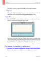
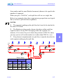
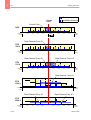
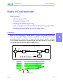
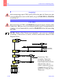
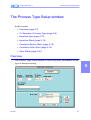
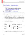
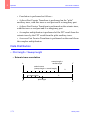
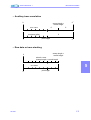
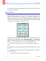
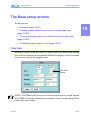
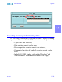
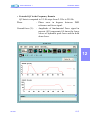
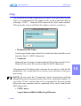
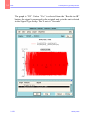
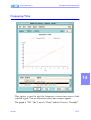
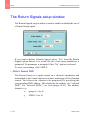
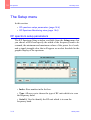
User’s Manual Vol. 1
TB in Radio or Dual telemetry
radio 0.58 s after the TB signal is received on the Blaster connector. The
FIRE signal is 120 ms long.
Adjusting the delay between F. O. and Firing (Explosive)
The purpose of this procedure is to adjust the delay between the Firing
Order sent to the source controller and the FIRE sent to the radio units
so that the TB of the source controller matches the T0 of the radio units.
The procedure is as follows:
• Connect the source controller to the BLASTER connector, or the
LSI, using FO and TB signals.
• In the Process Type Setup for the process type used (in the
Operation main window), set TB window to 1420 ms.
• Start an acquisition.
• After acquisition is complete, one of the following three cases may
arise:
- A window pops up with the message:
5
INTERNAL TB
TB occurred xxxx.xx ms after start
acquisition
OK
CANCEL
. Note the value xxxx.xx and choose CANCEL.
. In the Process Type Setup for the process type used (in the
Operation main window), set TB window to 1420+xxxx.xx ms.
- A window pops up with the message:
INTERNAL TB
TB occurred xxxx.xx ms before start
acquisition
OK
CANCEL
. Note the value xxxx.xx and choose CANCEL.
0311401
5-63
5
Operation
TB in Radio or Dual telemetry
. In the Process Type Setup for the process type used (in the
Operation main window), set TB window to 1420-xxxx.xx ms.
- No window pops up, that is the TB window is properly adjusted:
. Start an acquisition.
After acquisition is complete, no window should pop up: the difference
between the TB and the radio units T0 is less than 40 microseconds.
NOTE: If required, modify the settings of the source controller to have
a delay greater than 1420 ms between FO and TB.
5-64
January 2002
User’s Manual Vol. 1
Shooting with an LSS
Shooting with an LSS
In this section:
• Overview (page 5-65)
• Taking a shot with an LSI (page 5-66)
Overview
The LSS (Line Shooting System) allows you to use the 408UL
telemetry network rather than a radio link to synchronize a remote
shooting system with the recording truck, for example in situations and
over stretches of land where radio communications are difficult.
Shooting with an LSS does not require any audio communications
between the observer in the recording truck and the shooter. The LSS
consists of an LSI unit associated with an HSU.
LSI
5
LRU
HSU
You can connect another
shooting system on the second
Blaster connector
Blaster
controller
• The LSI (Line/Source Interface) allows you to connect a blaster
controller along an acquisition line instead of connecting it to the
control unit’s Blaster connector. It acts as a remote Blaster connector.
0311401
5-65
5
Operation
Shooting with an LSS
• The HSU (Hand-Shake Unit) is used by the shooter to supply the
status of the firing device and the number of the corresponding shot
point to the central unit.
For details on how to connect the HSU to the blaster controller, see
408UL Installation Manual.
Taking a shot with an LSI
• Prerequisites
1. The delay of the Time Break returned by the blaster controller,
following a Firing Order, is assumed known and invariable. It must be
entered into the TB Window field (see TB window on page 5-9). See
also Adjusting the delay between F. O. and Firing (Explosive) on
page 5-63.
2. To enable shooting with LSI units, you must select the “LSI”
option and the type of blaster in the Install main window. See Blaster
type (page 2-5).
With the LSI option enabled:
- the indicator LED on FDUs, otherwise used as a test result
indicator, is used to tell the shooter whether he is allowed to
connect/disconnect an LSI between two links.
- you cannot take a shot until retrieval of the previous one is
complete, whatever the field equipment and the shooting method
used.
3. Use the Shooter Setup menu to assign a Shooter name to each LSI
that may be connected and to specify the gain of the Uphole and CTB
channels. See The Shooter Setup window (page 5-36).
• Step-by-step operating instructions
The table below gives the step-by-step procedure for a shooter to insert
an LSI into the spread and for an observer in the recording truck to take
a shot using that LSI.
5-66
January 2002
User’s Manual Vol. 1
Operator
Shooting with an LSS
Action
Result
Observer
Go to “Field On” (unless already
done) in the Line main window.
Shooter
Locate the junction the two FDU
links where to insert the LSI, and
check to see if the indicator LED
on the FDUs is blinking.
When the indicator link is
blinking, disconnect the links and
connect the LSI in between.
Observer
Click on
in the Line
main window to view the LSI
units connected.
Shooter
Select the Shot Point number,
using the thumbwheel switch on
the HSU. Press Send button.
Observer
- Read Shot
Point No. sent
by shooter.
Blinking
Unplug
“Line OK”
LSI
“Connected” shooter in the
Operation main window.
Arm Set
Arm En
HSU
123456
Send
Indicator stops blinking on FDUs.
- Select shooter in Operation
main window.
“Arm enable” lights up.
Arm Set
Arm En
Spread is formed.
123456
Send
- Activate “Arm Enable”.
Shooter
Press “Arm set”
on HSU.
Arm Set
Arm En
123456
“Arm set” indicator in Operation
main window.
Send
Observer
Click on
in the Operation main window.
Observer
After Retrieve is complete,
deselect shooter.
Firing device is triggered. “Arm
set” goes out in Operation main
window. Acquisition is performed.
“Disconnect enable” lights up on
LSI.
LED on FDUs blinking again.
“Arm enable” goes out on HSU.
0311401
5-67
5
5
Operation
Shooting with an LSS
The Up-Hole and CTB (Confirmed Time Break) traces from the LSI are
placed ahead of the Auxiliary traces. They are acquired with the same
Sample Rate and filter type as seismic channels.
See “Source controller formats” in User’s Manual Vol. 2 for the fields
updated with the messages from the source controller.
5-68
January 2002
User’s Manual Vol. 1
More About Correlation
More About Correlation
In this section:
• Description (page 5-69)
• Data Distribution (page 5-72)
Description
Correlation in the 408UL involves two types of boards :
• FTP (up to 3 boards, each with two processors)
• MPM (two boards).
Correlation is achieved in the frequency domain, using the "Fast Fourier
Transform" method. It is performed on a set of data whose length is 2n,
greater than "Pilot length" or "Sweep length", whichever is the longest,
+ "Investigation length".
The results from the correlation process begin with positive time result
data and end with negative time result data.
Correlation may be performed on three types of traces :
• auxiliary traces
• seismic traces
• seismic traces in similarity tests.
• Correlation of auxiliary traces
Auxiliary trace correlation is performed by one of the processors on the
first FTP board. The following operations are allowed on an auxiliary
trace :
• Autocorrelation (e.g. aux1*aux1)
• Cross-correlation (e.g. aux2*aux1)
• Stack (e.g. aux3)
0311401
5-69
5
5
Operation
More About Correlation
For Autocorrelation or Cross-correlation, the second term in the
expression of the correlation operation stands for the Pilot trace.
• Autocorrelation and cross-correlation
Autocorrelation and crosscorrelation processings are identical. The
results consist of two traces : one for negative time shifts, one for
positive time shifts. Correlation is performed as follows :
• A direct Fast Fourier Transform is performed on the "pilot"
auxiliary trace, with this trace as real part and 0 as imaginary part.
• A direct Fast Fourier Transform is performed on the operand
auxiliary trace, with this trace as real part and 0 as imaginary part.
• A complex multiplication is performed of the result from the
operand auxiliary trace FFT by the result from the pilot auxiliary
trace FFT.
• A reverse Fast Fourier transform is performed on the result from
the complex multiplication.
• Stack
No correlation is performed on an auxiliary trace. Only stacking is
performed.
When two pilots are used, the results from auxiliary traces are located
in the two records.
The order in which the result traces are written to tape is in agreement
with the order of sequences in the description of the processings to be
done.
The negative-time trace always comes first.
• Correlation of seismic traces
Seismic trace correlation is performed by all FTP boards installed.
The following operations are allowed on seismic traces :
• Correlation with one auxiliary trace (1 pilot)
5-70
January 2002
User’s Manual Vol. 1
More About Correlation
• Correlation with two auxiliary traces (2 simultaneous pilots).
• Correlation with 1 pilot
Each correlated trace yields a single result trace (positive time).
• Correlation with 2 pilots
Each correlated trace yields two result traces :
• 1 trace results from correlation with the first pilot (positive time).
• 1 trace results from correlation with the second pilot (positive
time).
This gives rise to two records with the same trace count on tape.
If a trace is "dead", then all its samples are zeroed.
Correlation is performed as follows :
• A direct Fast Fourier Transform is performed on the "pilot"
auxiliary trace, with this trace as real part and 0 as imaginary part.
• A direct Fast Fourier Transform is performed on two seismic traces
with one seismic trace as real part and the other seismic trace as
imaginary part.
• A complex multiplication is performed of the FFT result from the
2 seismic traces by the FFT result from the pilot auxiliary trace.
• A reverse Fast Fourier Transform is performed on the result from
the complex multiplication.
• Correlation of seismic traces in similarity tests
Similarity tests are performed with a single source.
Correlation of seismic traces in similarity tests may be performed by
any of the FTP boards.
The result is in the form of two traces :
• 1 trace for negative time shifts
• 1 trace for positive time shifts.
0311401
5-71
5
5
Operation
More About Correlation
• Correlation is performed as follows :
• A direct Fast Fourier Transform is performed on the "pilot"
auxiliary trace, with this trace as real part and 0 as imaginary part.
• A direct Fast Fourier Transform is performed on the seismic trace,
with this trace as real part and 0 as imaginary part.
• A complex multiplication is performed of the FFT result from the
seismic trace by the FFT result from the pilot auxiliary trace.
• A reverse Fast Fourier Transform is performed on the result from
the complex multiplication.
Data Distribution
• Pilot length < Sweep length
• Seismic trace correlation
sweep length +
record length
0
seismic trace
(sweep length + record length)
aux trace (pilot)
2n
0
0
pilot length
0
5-72
2n
January 2002
User’s Manual Vol. 1
More About Correlation
• Similarity seismic trace correlation
0
2n
sweep length +
record length
seismic trace
0
0
aux trace (pilot)
0
pilot length
2n
• Auxiliary trace correlation
0
2n
sweep length +
record length
0
aux. trace
0
aux trace (pilot)
0
pilot length
5
2n
• Raw data or trace stacking
sweep length +
record length
0
seismic. trace
(sweep length + record0 length
aux trace
0
0311401
pilot length
5-73
5
Operation
More About Correlation
• Pilot length = Sweep length
• Seismic trace correlation
sweep length +
record length
0
seismic trace
(sweep length + record length)
aux trace (pilot)
2n
0
0
pilot length
0
2n
• Similarity seismic trace correlation
0
0
seismic trace
aux trace (pilot)
0
0
pilot length
5-74
2n
sweep length +
record length
2n
January 2002
User’s Manual Vol. 1
More About Correlation
• Auxiliary trace correlation
0
2n
sweep length +
record length
0
aux. trace
0
aux trace (pilot)
0
pilot length
2n
• Raw data or trace stacking
sweep length +
record length
0
seismic. trace
(sweep length + record
0 length
5
aux trace
0
0311401
pilot length
5-75
5
Operation
More About Correlation
• Pilot length > Sweep length and ≤ (Sweep length + Record
length)
• seIsmic trace correlation
pilot length +
record length
0
0
seismic trace
(sweep length + record length)
aux trace (pilot)
2n
0
0
pilot length
0
2n
• Similarity seismic trace correlation
0
0
seismic trace
aux trace (pilot)
0
0
0
pilot length
5-76
2n
pilot length +
record length
2n
January 2002
User’s Manual Vol. 1
More About Correlation
• Auxiliary trace correlation
0
2n
pilot length +
record length
0
aux. trace
0
aux trace (pilot)
0
pilot length
2n
• Raw data or trace stacking
pilot length +
record length
0
0
seismic. trace
(sweep length + record
0 length)
aux trace
0
0311401
5
0
pilot length
5-77
5
Operation
More About Correlation
• Pilot length > Sweep length and > (Sweep length + Record
length)
• Seismic trace correlation
pilot length +
record length
0
0
seismic trace
(sweep length + record length)
aux trace (pilot)
2n
0
0
pilot length
0
2n
• Similarity seismic trace correlation
0
0
seismic trace
0
5-78
0
0
aux trace (pilot)
0
2n
pilot length +
record length
pilot length
2n
January 2002
User’s Manual Vol. 1
More About Correlation
• Auxiliary trace correlation
0
2n
pilot length +
record length
aux. trace
0
0
aux trace (pilot)
0
pilot length
2n
• Raw data or trace stacking
pilot length +
record length
0
0
aux trace
0
0311401
seismic. trace
(sweep length + record length)
0
5
pilot length
5-79
5
Operation
5-80
More About Correlation
January 2002
Chapter
6
408UL User’s Manual
Volume 1
Noise Editing
This chapter describes the Noise Editing environment
This chapter includes the following sections:
• The main window (page 6-2)
• The Noise Editing Setup window (page 6-5)
• More About Noise Elimination (page 6-9)
• The Results pane (page 6-16)
0311401
6-1
6
Noise Editing
The main window
The main window
In this section:
• Overview (page 6-2)
• Auto/Manual (page 6-3)
• Hold/Var (page 6-3)
• Init Thresh (page 6-3)
• Load Thresh (page 6-3)
• Save Thresh (page 6-3)
Overview
6-2
January 2002
User’s Manual Vol. 1
The main window
Auto/Manual
Clicking "Manual" isolates the Noise Editing stage from the preceding
stage in the 408UL and enables local functions in this main window. As
a result, data acquisition will be suspended until you click "Auto".
Clicking "Auto" connects the Noise Editing stage to the preceding stage
in the 408UL and allows data acquisition and processing to be
performed.
Hold/Var
This button is used to enable or disable automatic updating of noise
editing thresholds in the "Historic" noise elimination process.
Clicking "Var" enables thresholds to be automatically updated.
Clicking "Hold" causes threshold to remain fixed at the latest value
updated before the "Hold" function was selected.
Init Thresh
Clicking "Init Thresh" presets all thresholds (64 windows) on all
channels on all threshold types (up to 16) to the initialization value
entered using the "Setup" menu, for "historic" noise elimination.
Load Thresh
Clicking "Load Thresh" restores the latest noise editing thresholds
saved, so that they can be used as initialization values in the next
"Historic" noise elimination process.
Save Thresh
Clicking "Save Thresh" saves all current noise editing thresholds so that
they can be used at a later date in "historic" noise elimination.
This command should be used prior to turning the power off or prior to
taking a shot with a different geometry which could affect noise editing.
0311401
6-3
6
6
Noise Editing
The main window
The "Save Thresh" command saves :
• the threshold types used after power-on, or after clicking "Init
Thresh" or "Load Thresh", until the next "Save Thresh" command is
initiated,
• the traces used in each threshold type,
• and the 64 windows on each trace (unused windows are initialized
at the threshold initialization value).
6-4
January 2002
User’s Manual Vol. 1
The Noise Editing Setup window
The Noise Editing Setup window
Prior to any processing, an offset correction operation is performed on
each sample:
n
A( k , i ) = A ( k , i ) −
6
∑ A( k , i )
k =1
n
The stack formula is given below as a reminder:
A( k , i ) =
0311401
s
∑ A( k , i , p)
p =1
6-5
6
Noise Editing
The Noise Editing Setup window
A(k)
=
kth sample
n
=
number of samples in the acquisition
i
=
trace index
p
=
stack index
s
=
current stack fold
• Noise Editing
(see also More About Noise Elimination (page 6-9)).
• HIST
If you click this toggle button the noise editing function is enabled.
Then you must define the set of parameters which are necessary to
remove impulsive noise using an historical type of editing.
• DIV stack
If you click this toggle button, then the Diversity Stack noise
elimination function is enabled. For this type of noise elimination, you
are not required to enter any parameter, apart from the Low Trace
Percentage, Low Trace Value and Nb of Windows.
The energy (E) from each trace is calculated by averaging the squares
of the samples (before correlation). Then each sample is multiplied by
the inverse of the energy previously computed.
At the end of n vibrations (end of Vibrated Point) each sample stacked
(before or after correlation) is multiplied by the inverse of the sum of
the inverses of the energies previously computed.
There's no peak editing function for that type of noise elimination. The
Diversity Stack function cannot be used in Stack-Only operation.
• OFF
If you click this toggle button, then the noise editing function is
disabled, and no parameters need to be defined.
6-6
January 2002
User’s Manual Vol. 1
The Noise Editing Setup window
• Editing Type
• Zeroing
If you click this toggle button then any sample equal to or greater than
the editing threshold will trigger the process which zeroes the samples
over a window length that is selected by the “Zeroing length”
parameter; linear-variation taper, over a window selected by the
“Zeroing taper length” parameter, is programmed before and after the
zeroed portion to prevent discontinuity.
• Clipping
If you click this toggle button then every sample equal to or greater than
the threshold will be clipped to the editing threshold value by the noise
editing process.
• Nb of Windows
(Allowable range: 1 to 64). Number of noise editing windows.
With the noise elimination function activated, the acquisition length
may be divided into one or more windows (1 to 64).
With "Diversity Stack" noise elimination and the "Correlation Before
Stack" processing option, a single window is used.
• Zeroing Taper Length
2n (allowable range for n: 0 to 8). This parameter represents the number
of samples corresponding to the linear-variation taper length before and
after a zeroed window, when the “ZEROING” option is selected for the
“Editing type” parameter.
• Zeroing Length
(Allowable range: 1 to 500 milliseconds). Zeroing window length when
a sample exceeds the editing threshold, when the “ZEROING” option is
selected for the “Editing type” parameter.
0311401
6-7
6
6
Noise Editing
The Noise Editing Setup window
• Threshold Init Value
(Selectable from 0 to -132 in 6-dB steps). Initialization value for all
noise editing thresholds and threshold types in all windows of every
channel, for “Historic” noise elimination.
• Low Trace
(Selectable from 0 to 100%). Decision criterion for Low channel
detection. If the percentage corresponding to the number of samples
which are less than the “Low trace value” parameter exceeds this limit
then the trace is reported as “low” in the “Results” pane.
If a trace is "low", threshold update is not performed at the end of the
sweep.
• Low Trace Value
(Selectable from 0 to -132 in 6-dB steps). Upper limit for “Low”
channel detection. If a channel sample is less than or equal to this limit,
then the low channel process is triggered for the corresponding channel.
• Noisy Trace %
(Selectable from 0 to 100). Decision criterion for noisy channels. If the
percentage corresponding to the number of zeroed or clipped samples
(percentage computed with respect to the acquisition length) exceeds
this parameter value then the trace is considered as noisy.
The corresponding trace number is simply reported in the "Results"
pane and in the observer's log. No further action is taken (i.e.normal
threshold updating takes place).
6-8
January 2002
User’s Manual Vol. 1
More About Noise Elimination
More About Noise Elimination
In this section:
• "Spike Editing" method (page 6-9)
• Diversity Stack (page 6-12)
"Spike Editing" method
The SPIKE EDITING method removes all samples exceeding a special
threshold.
The traces are processed successively in the order generated by the
acquisition process. Acquisition is performed line by line (from LOW
to HIGH receiver positions), starting with the farthest LEFT line.
The first trace is therefore the farthest in the LOW branch, in the farthest
LEFT line.
When the number of traces increases (ROLL IN), the new traces are
initialized with the value of the "THRESHOLD INIT VALUE"
parameter.
When the number of traces decreases (ROLL OUT) it is the last ones
which disappear.
Each trace is divided into several time windows whose length is equal
to ACQUISITION LENGTH/NUMBER OF WINDOWS.
The maximum number of windows for each trace is 64.
Each window has its own threshold, expressed as a multiple of 3 dB.
Every acquisition with the same length and energy spreading can be
associated with the same threshold type (i.e. if the initial phase only is
different). If acquisition types with different lengths or energy levels are
used, they must be associated with different threshold types.
There may be up to 16 different threshold types.
Two aspects are to be considered in the processing of a trace : removal
of samples exceeding a threshold, and threshold updating.
0311401
6-9
6
6
Noise Editing
More About Noise Elimination
• Removal of samples exceeding a threshold
Two methods may be used:
• Zeroing
With this method, any sample greater than or equal to the threshold
causes a number of samples to be zeroed.
The number of zeroed samples is specified by ZEROING LENGTH,
and the zeroing process is brought in and removed gradually, i.e.
beginning and ending with a "linear-variation taper".
The TAPER LENGTH is expressed as a number of samples and equal
to a power of 2.
• Clipping
Any sample exceeding the threshold is cut down to the value of the
threshold.
• Threshold updating
In each window, the threshold is updated with respect to the highest
sample in the window.
Threshold updating is performed at the end of the noise elimination
process, using the RANGE parameter (12 dB) as follows (see also
diagram below):
• Highest sample within D area:
If Threshold-3dB-Range > Highest sample, then Threshold is decreased
3dB.
• Highest sample within C area:
If Thresh -3dB > Highest sample ≥ Thresh-3dB-Range, then Threshold
is unchanged.
• Highest sample within B area:
If Threshold > Highest sample ≥ Threshold-3dB, then Threshold is
increased 3 dB.
6-10
January 2002
User’s Manual Vol. 1
More About Noise Elimination
• Highest sample within A area:
If Highest sample > Thresh and VP's 1st acquisition complete, then
Threshold is increased 3 dB.
Thr.
A
A
A
A
B
3 dB
B
B
B
C
Range
12 dB
C
C
C
D
D
D
-3 dB
D
Thr.-3dBRange > max
sample
Thr.-3dB
> max sample
≥Thr-3 dB-
Thr> max
sample ≥ Thr.3dB
max
sample >Thr.
• Special cases
Threshold updating is not performed:
- if the trace is reported "LOW"
6
- if the HOLD option, rather than VAR, is selected
- if the trace is "dead" (corrupted)
A trace is LOW if, before noise elimination, the percentage of samples
which are smaller than the specified LOW TRACE VALUE exceeds
the specified LOW TRACE %.
0311401
6-11
6
Noise Editing
More About Noise Elimination
Diversity Stack
The DIVERSITY STACK method depends on the CORRELATION
AFTER STACK/ CORRELATION BEFORE STACK option selected.
• Correlation After stack
Each trace is divided into several windows whose length equals:
AcquisitionLength
---------------------------------------------------NumberOfWindows
The maximum number of windows for each trace is 64.
The entire processing is performed before correlation but includes two
parts: before stacking and after stacking.
A(k) = kth sample
n
= number of samples in the window
i
= trace index
j
= window index
p
= current stack fold
• Processing before stack
For each window in a trace, the following computation is performed:
E (i , j , p ) =
n
∑
[ A( k ) ]
k =1
2
n
On the first window, the following computation is performed:
1 A ( k ) Q -------------------E ( i, j, p )
6-12
January 2002
User’s Manual Vol. 1
More About Noise Elimination
On the subsequent windows, a ramp is applied to the samples:
• Computation of the ramp increment (S) for a window:
E ( i, j, p ) – E ( i, j – 1, p )
S ( j ) = --------------------------------------------------------n
• Processing on the samples:
A(k)
-------------------------------------------------------E ( i , j – 1, p ) + S ( j ) Q k
where (1 ≤ k ≤ n).
Assuming the current stack fold is p, when the whole ith trace is
computed the following computation is performed on all the E(i,j,p)
terms for each window:
1
1
--------------------- + -----------------------------E ( i, j, p ) E ( i, j, p – 1 )
6
• Processing after stack
Assuming m is the last stacking fold prior to writing to tape, the
following computation is performed:
On the first window, the following computation is performed:
A( k ) ∗
1
m
∑
p =1
0311401
1
E (i , j , p)
6-13
6
Noise Editing
More About Noise Elimination
On the subsequent windows, a ramp is applied to the samples:
• Computation of the ramp increment (S) for a window:
1
m
S ( j) =
∑
p =1
1
E (i , j , p)
−
1
m
1
E (i , j − 1, p)
∑
p =1
n
• Processing on the samples:


A( k ) ∗ 



1
m
∑
P =1
1
E (i , j − 1, p)
+
[


S ( j) ∗ k 



]
where (1 ≤ k ≤ n).
• Correlation Before stack
Each trace is processed as a single window whose length equals the
ACQUISITION LENGTH.
The processing includes two sequences, one before correlation, another
after correlation.
• Processing Before correlation
A(k) = kth sample
6-14
n
= number of samples in the acquisition
i
= trace index
p
= current stack fold
January 2002
User’s Manual Vol. 1
More About Noise Elimination
For each trace, the following computation is performed:
n
E (i , p) =
∑
[ A( k )]
2
n
k =1
1
A ( k ) Q ---------------E ( i, p )
• Processing After correlation
assuming m is the last stacking fold before writing to tape, the following
computation is performed:
C (i ) =
1
m
∑
p =1
1
E (i , p)
Finally, for each trace i, each sample is multiplied by C(i).
See also More About Correlation (page 5-69).
6
0311401
6-15
6
Noise Editing
The Results pane
The Results pane
The “Results” pane provides information on “Low” or “Noisy”
traces.”Line” and “Receiver” respectively indicate a Line number and
Receiver Position number for which one or more Low or Noisy stack
has been encountered.
“Nb of stacks low” and “Nb of stacks Noisy” respectively indicate the
count of stacks during which the trace identified was low or noisy for
the latest Vibrated Point.
Clicking "Freeze" prevents the Results pane from been updated until
you click "Freeze" again.
6-16
January 2002
Chapter
7
408UL User’s Manual
Volume 1
Recorder
This chapter describes the RECORDER environment
This chapter includes the following sections:
• The main window (page 7-2)
• The Tape Setup window (page 7-3)
• The Tape Transport Configuration setup window
(page 7-5)
• Auto/Manual (page 7-7)
• Function Buttons (page 7-11)
• Results (page 7-16)
0311401
7-1
7
Recorder
The main window
The main window
In this section:
• Overview (page 7-2)
• File (page 7-2)
Overview
This environment is dedicated to recorder controls.
File
Load / Save
This button allows all of the current parameters that have been set up for
the entire environment to be saved to or loaded from a named file. This
feature can be useful for storing configurations that have to be used
periodically.
Warning: After installing a new software release, do not load any
parameters from files saved with earlier releases.
7-2
January 2002
User’s Manual Vol. 1
The Tape Setup window
The Tape Setup window
• Record Nb
(Allowable range: 0 to 999 999).
Allows you to specify an identification # for the next seismic
acquisition record on tape.
• Test Record Nb
(Allowable range: 0 to 999 999).
Allows you to specify an identification # for the next test record on tape.
WARNING
Be sure to choose adequate values as Record Nb and Test Record Nb.
To preclude any conflict, the two types of record numbers should lie
within two distinct ranges of values.
0311401
7-3
7
7
Recorder
The Tape Setup window
• Tape Nb
(Allowable range: 0 to 9999).
Allows you to specify a reel tape number to be recorded in the header
block of the next records. It is automatically incremented after the Burst
is written on tape.
• Tape Label
(16 ASCII characters max.).
Used to enter a user-friendly name for the reel tape #.
• Files per tape
(Allowable range: 1 to 9999).
Allows you to specify the maximum number of records that may be
written to a tape.
7-4
January 2002
User’s Manual Vol. 1
The Tape Transport Configuration setup window
The Tape Transport Configuration setup
window
• Tt Mode
This option button allows you to specify the recording mode:
Single: seismic data is recorded on a single Tape Transport (the first
reported "ready", i.e. shown in orange in the Device pane, if two or
more recorders are connected).
Simult: seismic data is recorded on two tape transports concurrently (the
first two reported "ready", i.e. shown in orange in the Device pane, if
two or more recorders are connected).
• Init
This pushbutton is used to reset the SCSI bus (e.g. if you power up a
recorder after powering up the HCI, or in the event of fatal error on the
SCSI bus).
7
• SEGD Trace Blocking (CMXL users only)
To improve the system cycle time, you can shorten the record time by
activating the Trace Blocking option. With that option enabled, several
traces are grouped to form a single block limited to 256 kilobytes.
See SEGD format in 408UL User’s Manual Vol. 2. See also 408UL
User’s Manual Vol. 3 (Utilities).
0311401
7-5
7
Recorder
The Tape Transport Configuration setup window
Unless you choose the trace blocking option, the system will record
traces to tape as individual blocks separated by a gap.
When you play back any record on the 408UL, the system automatically
chooses the appropriate option.
7-6
January 2002
User’s Manual Vol. 1
Auto/Manual
Auto/Manual
In this section:
• General (page 7-7)
• AUTO Mode (page 7-8)
• AUTO Mode (page 7-8)
General
Clicking “MANUAL” enables the recorder’s local control functions
(INIT, EOF, AGAIN, PLAYBACK) and isolates the recorder stage
from the preceding stage in the 408UL. As a result, data acquisition may
be suspended (when the preceding stages are full) until the recorder is
reset to AUTO.
Clicking "AUTO" inhibits the recorder’s local control functions and
connects the recorder stage to the preceding stage in the 408UL. Up to
4 recorders (identified as Device numbers 0 to 6) can be connected on
the SCSI bus. As soon as a recorder is connected on the bus and
powered up, an indicator light shows up in the "Device" pane, along
with the Device number assigned by the user to that recorder. (The
Device number is entered by the user on the recorder). The indicator
light is :
- not shown : if the recorder is not connected or not powered up,
- red : if the recorder is connected and powered up, but no
cartridge is inserted,
- orange : if the recorder is connected and powered up, with a
cartridge inserted (the tape is at the BOT),
7
- green : if the recorder is connected and powered up, with a
cartridge inserted and currently used for recording.
0311401
7-7
7
Recorder
Auto/Manual
AUTO Mode
When data is available from the preceding process stage, 1 (if "Single"
activated) or 2 (if "Simult" activated) recorders are selected from those
ready (i.e. with an orange indicator). The indicator of each selected
recorder turns green.
A recorder can be selected if :
- its cartridge is blank
- its cartridge is not blank but the tape is positioned at the end of
the last record. (This can be done using the PLAYBACK Last
Record function in MANUAL mode).
If any recorder is required but cannot be selected, a message shows up
in the "Status" pane :
- "Waiting for device ready" (if no cartridge is inserted).
- or "Device n not at end of last record" (if a non-blank cartridge
is inserted).
The indicator of each recorder selected and used for recording remains
green so long as the recorder is in use, and turns red when the cartridge
is ejected :
- manually by the operator
- or automatically when the 408UL "File Count" is equal to the
"File per Tape".
If Tape ByPass is activated, acquisition is performed regardless of the
state of the recorders, and both the "Results" and "Status" panes remain
blank.
Any cartridge that is write-protected or closed by a second EOF is
ejected and a message appears in the "Status" pane.
In the event of erroneous record, a dialog box shows up allowing you to
select :
- RETRY : the 408UL re-writes the record on the selected
recorder (Single) or recorders (Simult).
7-8
January 2002
User’s Manual Vol. 1
Auto/Manual
- MANUAL : it is for you to decide whether or not the record
should be written again.
A dialog box shows up whenever you are required to confirm the
current situation, that is :
- if Tape Bypass is activated
- if the last record ended with an error : if you confirm then the
data is no longer available in the preceding process stage and
therefore cannot be recorded by the AGAIN function.
MANUAL MODE
You need to manually select the recorder you wish to work with, by
clicking the desired device icon. Any manual operation (PLAYBACK,
AGAIN, etc.) will be performed only on this recorder regardless of
whether the Single or Simult mode is activated.
• AGAIN
Can be used in the same way as in the AUTO mode.
• EOF
An EOF can be written anywhere on the tape. To write a second EOF
after the last record on the tape, you need to use the PLAYBACK "Last
Record" function beforehand.
• PLAYBACK
The “Results” pane displays a line starting with “Search” for each
Record Header read, and a Playback line while the record is being
played back. The PLAYBACK “Last Record” function allows you to go
on recording on a cartridge that is not blank, unless it is closed by a
double EOF. See Help on functions.
If you switch from MANUAL to AUTO and DATA is activated, then a
warning box shows up displaying :
- the next TAPE number,
0311401
7-9
7
7
Recorder
Auto/Manual
- the next RECORD number,
- the next TEST RECORD number so that the operator can see if
the correct tape is loaded, and properly positioned.
7-10
January 2002
User’s Manual Vol. 1
Function Buttons
Function Buttons
• Data/tape Bypass
Clicking " Data " enables the normal record and read-after-write
function.
Clicking "Tbp" (Tape Bypass) enables data to be dumped to the camera
without recording to tape. The selection can be changed only when
MANUAL is activated.
With the SCSI recorder type, the "Results" pane is blank if "Tape
Bypass" is activated.
• FILE BUTTON
When the "File" button is activated, clicking the "Again" button opens
a dialog box used to save the contents of the latest record (i.e. latest
shot) to the hard disk, so that it can be analyzed at a later date, with the
VQC software for example. Only the latest files thus generated are kept
on the hard disk, depending on the free disk space (they can be accessed
through the File Manager).
The dialog box (MEDIA.VIEW) displays the available disk space for
the file to be saved, and contains a list box showing the name and size
of the files already saved.
- The DELETE key allows you to erase any file selected by
clicking in the list.
0311401
7-11
7
7
Recorder
Function Buttons
- The DIR key displays the file name list again
- The "File" Name text box is used to enter a name for the file (i.e.
record) to be saved.
- Clicking GO causes the record to be saved to the disk (into the
directory export/home/sn408Hci/segd).
• EOF
Clicking this pushbutton causes a second End of File to be written after
the latest one. (An EOF is automatically written at the end of each
record). The second EOF is usually interpreted as the end of the tape.
This resets the file count to 0.
NOTE: Two EOF’s in succession are automatically recorded when the
end of tape is sensed in the course of a record or when the file count
reaches the “File per Tape” count. If simultaneous recording on two
tape transports is selected (in the Tape Transport Configuration setup
dialog box) then a double EOF is written on both tape transports.
• AGAIN
Clicking this pushbutton causes the same record to be written again (to
a new tape, for example, after a failure to write the complete record).
The Record Number is automatically incremented.
With the "Data" button activated, clicking AGAIN causes the record to
be written again to tape. With the "TBP" button activated, clicking
AGAIN causes the record to be played back on the camera (if any).
With the "File" button activated, clicking "AGAIN" opens a dialog box
(MEDIA VIEW) displaying the available disk space for the file to be
saved, and containing a list box showing the name and size of the files
already saved.
- The DELETE key allows you to erase any file selected by
clicking in the list.
- The DIR key displays the file name list again.
7-12
January 2002
User’s Manual Vol. 1
Function Buttons
- The "File" Name text box is used to enter a name for the file (i.e.
record) to be saved.
- Clicking GO causes the record to be saved to the disk (into the
directory export/home/sn408Hci/segd).
• PLAYBACK
Clicking this pushbutton opens a dialog box that allows you to select the
Playback Type from an option button:
7
0311401
7-13
7
Recorder
Function Buttons
Parameter
Description
Last Record
Used for a playback of the preceding record. The tape will
be wound back then forward so as to find a header with a
Record Number matching the Record Number of the latest
file recorded. This function is also used to position the tape
at the end of the latest record and enable switching to
"AUTO". Playback will start as soon as the expected
header is encountered.
Next Record
Used for a playback of the next record. Whatever the
position of the tape, the recorder will perform a forward
search for the next record header and start the playback as
soon as a header is encountered.
Forward
The record to be played back is assumed to be located
AFTER the current position on the tape. You have to
specify the desired record number in the "Search Nb" text
box. The recorder will perform a forward search for the
header of the specified record. When the header is
encountered, the recorder will wind back the tape into the
gap preceding the header and restart forward, to read the
header again, and perform playback.
Backward
The record to be played back is assumed to be located
AHEAD OF the current position on the tape. You have to
specify the desired record number in the "Search Nb" text
box. The recorder will perform a backward search for the
header of the specified record, then, when the header is
encountered, perform playback.
NOTE : The header cannot be read backward. Instead, on
each EOF encountered during the backward search, the
next header is read forward, and the backward search
continues until the desired header is encountered.
Click APPLY after selecting the desired option.
Clicking GO starts the playback.
Clicking ABORT terminates the playback in the search phase.
The file Number of each record encountered during the search phase is
displayed in the “Results” pane.
7-14
January 2002
User’s Manual Vol. 1
Function Buttons
• PLOTTER
The PLOTTER button is only available if an OYO GS612 plotter is
installed. It performs the same function as the PRINT key on the plotter.
The PLOTTER button cannot be used (i.e. is dimmed) unless
MANUAL is activated.
7
0311401
7-15
7
Recorder
Results
Results
The "Results" pane provides the following information messages:
• Type
RECORD/PLAYBACK/SEARCH/AGAIN
- RECORD is displayed on completion of each data record when
AUTO is activated.
- PLAYBACK is displayed at the beginning of a playback
operation.
- SEARCH is displayed on each header read or searched for.
- AGAIN is displayed on completion of a record initiated by the
AGAIN pushbutton, with MANUAL activated.
• Device
Unless Tape Bypass is selected, the “Device” column contains the
number of the tape transport to which the data is written (two lines for
each record in Simult mode).
• Tape
Identification number of the tape currently used, incremented on the
first record written to the tape.
• File
Identification number of the latest record written to the tape, or played
back, or searched for.
• Count
Number of records written to or read from the current tape. This number
is automatically reset to 0 when a double EOF is recorded (manually or
when File Count = File per Tape) or when a blank cartridge is loaded.
7-16
January 2002
User’s Manual Vol. 1
Results
• Example of results
For each record written to a tape, an information line shows up in the
"Results" pane, as shown in the example below. (Nothing is displayed
when writing an EOF).
Type
Device
Tape
File
Count
Record
0
47
9001
1/20
first record on tape 47
Record
0
47
9020
20/20
last record on tape 47
Record
1
48
9021
1/20
first record on tape 48
7
0311401
7-17
7
Recorder
7-18
Results
January 2002
Chapter
8
408UL User’s Manual
Volume 1
Plotter (CM408 users)
This chapter describes the Plotter environment in
configurations with CM408 control modules.
This chapter includes the following sections:
• The main window (page 8-2)
• The Option menu (page 8-4)
• The AGC SETUP pane (page 8-6)
• The CAMERA pane (page 8-12)
• The PLOT SELECTION pane (page 8-14)
• The Plot Group Type setup window (page 8-18)
• The AGC On Properties setup window (page 8-16)
0311401
8-1
8
Plotter (CM408 users)
The main window
The main window
In this section:
• Overview (page 8-2)
• File (page 8-3)
Overview
8-2
January 2002
User’s Manual Vol. 1
The main window
This environment is dedicated to selection of parameters that define
what is displayed on monitor records and how it appears. There are two
operating modes, manual and automatic.
Manual mode is the simplest method of control, but requires that the
observer select all playback characteristics to suit the signal type before
the record is plotted. Automatic mode requires more effort to program
initially, but once set up switches between different sets of playback
parameters without any user intervention
The PLOTTER software is dedicated to processing the geophysical data
(scaling, filtering, AGC) for plotters and cameras. It supports 12'' and
24'' Plotters (selection should be made in the HCI Install window).
It performs the conversion to graphic data (rasterisation) in order to
print it out.
Traces are numbered from bottom to top, Aux traces at the top.
File
Load / Save
This button allows all of the current parameters that have been set up for
the entire environment to be saved to or loaded from a named file. This
feature can be useful for storing configurations that have to be used
periodically.
Warning: After installing a new software release, do not load any
parameters from files saved with earlier releases.
8
0311401
8-3
8
Plotter (CM408 users)
The Option menu
The Option menu
The PLOTTER main window allows you to choose different AGC and
plot parameters depending on the type of input data and on the type of
processing. The “Option” menu allows you to choose the way of setting
the AGC and plot parameters: automatic or manual.
See:
• AUTO option (page 8-4)
• MANUAL option (page 8-5)
AUTO option
With this option a Plot Selection pane is available that allows you to
choose one or more types of input data and save your choice, along with
the settings in the AGC SETUP and CAMERA panes, as a Plot Type in
the lower pane. As a result, the system will automatically use the
parameters specified in the AGC SETUP and CAMERA panes
whenever the type of input data and the type of processing used match
the selections made in the “Plot Selection” pane.
To generate a Plot Type:
• Make the desired selections in the three upper panes.
• Enter a Plot Type number into the "Nb" text box (You may enter a
Label in the "Label" text box).
• Click "Add". As a result, the new Plot Type is added into the list
box, unless it already exists. Use "Change" or "Delete" to make any
changes needed.
• Click "Apply". As a result, all Plot Types contained in the list box
are transmitted to the RECORDER environment.
Depending on the type of input data and on the type of processing used,
the system will automatically choose the appropriate Plot Type, so long
as "Auto" remains activated.
8-4
January 2002
User’s Manual Vol. 1
The Option menu
MANUAL option
With the Manual option, all Plot Types generated with the Auto option
are ignored. Only the AGC SETUP and CAMERA panes are available.
When you click "Apply" in the Plotter main window the parameters
selected in the AGC SETUP and CAMERA panes are transmitted to the
RECORDER environment and used so long as "Manual" remains
activated.
8
0311401
8-5
8
Plotter (CM408 users)
The AGC SETUP pane
The AGC SETUP pane
In this section:
• General (page 8-6)
• AGC Off (page 8-7)
• AGC On (page 8-8)
• Sample normalization for a camera (page 8-10)
General
The AGC SETUP pane allows you to select the following AGC
parameters (parameters that need to be adapted to the type of input data
or type of processing, unlike those selected in the AGC-ON
PROPERTIES dialog box in the Setup menu).
• AGC
This option button is used to enable or disable AGC. See AGC Off
(page 8-7) and AGC On (page 8-8).
• Pb Auxiliary Gain
Gain applied to Auxiliary traces during plots. Expressed in decibels,
selectable in 6-dB steps from 0 to 180 dB.
• Low cut
(Allowable range: 10 to 500 Hz). If you wish to set a low-cut filter for
the plot, activate the Low Cut check box and type the desired low-cut
frequency in the associated text box. If you wish to remove the filter,
leave the check box unchecked.
• High cut
(Allowable range: 30 to 500 Hz). If you wish to set a high-cut filter for
the plot, activate the High Cut check box and type the desired high-cut
8-6
January 2002
User’s Manual Vol. 1
The AGC SETUP pane
frequency in the associated text box. If you wish to remove the filter,
leave the check box unchecked.
• Notch
(Allowable range: 30.0 to 500.0 Hz). If you wish to set a notch filter for
the plot, activate the Notch check box and type the desired notch
frequency in the associated text box. If you wish to remove the filter,
leave the check box unchecked.
NOTE: The above three parameters (Low Cut, High Cut, Notch) are not
applied to Auxiliary traces.
AGC Off
The seismic traces have a fixed gain (Off Fixed Gain) unless a Linear
Gain Slope other than zero is selected, in which case the Off Fixed Gain
will increase during the plot by the Linear Gain Slope every second. The
auxiliary traces are always in fixed gain (PB Auxiliary Gain).
• OFF Fixed Gain
8
0311401
8-7
8
Plotter (CM408 users)
The AGC SETUP pane
Fixed gain applied when the AGC is off during camera plots. Expressed
in decibels, selectable in 6-dB steps from 0 to 180.
• Linear Gain Slope
Selectable from 0 to 48 in 1-dB steps. With no AGC, the amplitude at
the beginning of the trace is much higher than that at the end. To
compensate for that difference in amplitudes, a linear gain varying
linearly (with a fixed rate specified by the Linear Gain Slope parameter)
from the beginning of the trace to the end, is applied to all traces. The
relative amplitudes of the traces are preserved (unlike with AGC ON).
AGC On
The seismic traces have a fixed gain (Early gain) until their amplitudes
are released (Release time + Slope). Then the gain of each trace can
increase (maximum 96 dB) and decrease depending on their level and
on Setup parameters. See also The AGC On Properties setup window
(page 8-16). The auxiliary traces are always in fixed gain (PB Auxiliary
Gain)
.
8-8
January 2002
User’s Manual Vol. 1
The AGC SETUP pane
• Early Gain
Early gain applied to Seismic traces until they are released, during plots,
when AGC is on. Expressed in decibels, selectable in 6-dB steps from
0 to 180.
• Release Time
(Allowable range: 0 to 9999 ms). Period of time for which the Early
Gain is applied to the nearest seismic traces during plots when AGC is
on. The nearest traces from the source (according to Source location
from the Operation table) are released at the end of the Release time and
then the next traces are released every <Slope> milliseconds.
• Slope
(Allowable range: 0 to 999 ms). Increment per trace, to be added to the
Release Time, scaled by the Spacing Ratio. See The AGC On
Properties setup window (page 8-16).
• Wz Velocity
(Allowable range: 1 to 99999 m/s). With AGC on, if you activate the
associated GEOGRAPHIC button, a “Wz Velocity” text box is
available that allows you to specify the propagation velocity of the shot
wave in the ground. This will enable the system to calculate the time
when the AGC should be applied to the traces on the plotter, if the
source-to-receivers distances are known, instead of using the Release
Time and Slope parameters. The source-to-receivers distances are
calculated from the geographic locations of the receivers and the source
COG recorded in the SEGD header if the option is enabled (See the
Crew Setup in the GO 408 main window).
NOTE: By default the source-to-receiver distance is assumed
determined in metres, therefore the velocity in metres/second. If the
distance is determined in any other unit, then the velocity you enter
should be expressed in the corresponding unit instead of m/s (the unit
must be consistent with SPS data).
0311401
8-9
8
8
Plotter (CM408 users)
The AGC SETUP pane
Sample normalization for a camera
On a camera each sample is represented with an 8-bit data word (+127,
- 128). The normalization process is expressed by the following
formula:
Data sample × 127
Camera sample = --------------------------------------------K
where K is a coefficient that may assume different values, depending on
the process type and on the noise elimination method used for the trace.
• Process Type = Impulsive
K = max. sample value = 8388607
i.e. (223- 1)
• Process Type = Impulsive Stack
K = 8388607 x (Stacking fold)
• Process Type = Vibro Stack
• Noise elimination mode = Diversity
K = 8388607
• Noise elimination mode = Off or Historic
K = 8388607 x (Stacking fold)
• Process Type = Correl Before
• Noise elimination mode = Diversity
2
K = 1
--- ( 8388607 × number of pilot samples )
2
• Noise elimination mode = Off or Historic
2
K = 1
--- ( 8388607 × number of pilot samples ) × ( Stacking fold )
2
8-10
January 2002
User’s Manual Vol. 1
The AGC SETUP pane
• Process Type = Correl After
• Noise elimination mode = Diversity
2
1
K = --- ( 8388607 × number of pilot samples ) × ( Stacking fold )
2
• Noise elimination mode = Off or Historic
2
2
1
K = --- ( 8388607 × number of pilot samples ) × ( Stacking fold )
2
8
0311401
8-11
8
Plotter (CM408 users)
The CAMERA pane
The CAMERA pane
The CAMERA pane is used to select the following parameters:
• Plot Group Selection
If one or more trace group types have been defined in the Setup menu
(Plot Group Type Setup, page 8-18), then one or more buttons are
available in the Plot Group Selection box allowing you to select the
trace groups you wish to plot (up to 16 groups can be programmed). If
several have to be selected they must be in consecutive order (no gap).
• Plot All Groups option button
• No: A single group (selected with one of the Plot Group selection
buttons) is plotted at the end of each shot. If two or more trace groups
are selected, one is plotted at the end of one shot, another one at the
end of the next shot, etc.
8-12
January 2002
User’s Manual Vol. 1
The CAMERA pane
• Yes: all the trace groups selected with Plot Group Selection buttons
are plotted at the end of a shot, then every "n" shots (where "n" is
specified in the "Plot Recur." text box.
• Pagination type Nb
(Allowable range: 1 to 16). Allows you to specify the pagination Type
to be used (Pagination Types are generated in the LOG main window,
using the Setup menu). This determines the camera banner that will be
printed ahead of the plot.
• Direction
This option button allows you to select the Camera Banner orientation
(Portrait/Landscape).
8
0311401
8-13
8
Plotter (CM408 users)
The PLOT SELECTION pane
The PLOT SELECTION pane
The PLOT SELECTION pane appears only if the “Auto” option is
selected (see page 8-4). It allows you to specify the types of data and
processing for which the parameters selected in the AGC SETUP and
CAMERA panes should be used.
The types of data may be :
•Normal:
Normal acquisition
•Field Noise: Acquisition with no Firing Order
•SU Noise:
Noise due to station units
•Sine Wave: Sine wave test signal
•Impulse:
Impulse test signal
•Similarity:
Similarity test signal
•Synthetic:
Synthetic test signal.
The types of processing may be:
8-14
January 2002
User’s Manual Vol. 1
•Raw :
The PLOT SELECTION pane
no processing is performed
•Correl/stack : correlation and/or Stacking is performed.
NOTE: You are allowed to select more than one type of data and/or
processing for each Plotter Setup.
8
0311401
8-15
8
Plotter (CM408 users)
The AGC On Properties setup window
The AGC On Properties setup window
This dialog box allows you to set AGC parameters that do not need to
be adapted to the type of input data or type of processing (unlike those
selected in the main window):
These parameters cause the gain to change according to the following
scenario: the AGC phase starts after the trace is released. Its initial gain
is zero. Then, in the beginning, it can only increase in 6 dB steps if the
successive samples are below the lower threshold (1/4 of half full scale
if Threshold =12 or 1/8 of half full scale is Threshold =18) during a
time equal to Recovery Delay. Afterwards it can decrease in 6 dB steps
if the successive samples are higher than the upper threshold (half full
scale).
• Spacing Ratio
(Allowable range: 0.00 to 99.99).
NOTE: This parameter is not used if the Geographic option is activated
(in the main window’s AGC Setup pane).
This is a LINE spacing to RECEIVER POSITION ratio. Dimensionless
figure computed using the formula:
Line spacing (m) - × -------------------------------------------------1
Spacing Ratio = ------------------------------------------------------Line number increment Receiver spacing (m)
8-16
January 2002
User’s Manual Vol. 1
The AGC On Properties setup window
This factor is applied to the Slope parameter determining the way the
trace amplitude is released as a function of the location of the shot point
within the lines. See page 8-9.
Example: if Receiver Position spacing = 50 m and Line Position
spacing = 400 m with a line number increment equal to 10, then Spacing
Ratio = 0.8.
Default Value in 2D: As there is only one line in 2D, the Spacing Ratio
should be set to 0.
• Threshold
Lower threshold used to trigger an expansion command in the AGC
process:
• 12 dB
: 1/4 half full scale.
• 18 dB
: 1/8 half full scale.
• Recovery Delay
(Allowable range: 0 to 999 ms). Minimum time for which the signal is
below the lower threshold (signal <1/4 or 1/8 half full scale) before
triggering an expansion command in the AGC process.
• Compression Delay
(Allowable range: 0 to 99 ms). Minimum time for which the higher
threshold is exceeded (signal > 1/2 full scale) before triggering a
compression command in the AGC process.
NOTE: 0 stands for infinite delay.
8
0311401
8-17
8
Plotter (CM408 users)
The Plot Group Type setup window
The Plot Group Type setup window
In this section:
• Plot Group Type parameters (page 8-18)
• To generate a Plot Group Type setup (page 8-20)
Plot Group Type parameters
This window allows you to set plot parameters for the camera. For a
detailed description of plot parameters, see the camera or plotter
manufacturer's documentation.
8-18
January 2002
User’s Manual Vol. 1
The Plot Group Type setup window
• Line Select
You can select the number of lines to be plotted. This is helpful if the
number of channels is not the same in all lines or all records (rolling in,
rolling off). The Plot Start Line (order acquisition number) and Total
Seismic Line must be supplied. Warning: this selection is not working
if the line description has changed or is unknown (as could be the case
for a playback). In that case the following status is displayed: Group
line selection feature not available.
• Channel Select
You can select the total number of traces to be plotted with Plot Start
Channel, Channel Increment and Total Seis. Channels.
8
0311401
8-19
8
Plotter (CM408 users)
The Plot Group Type setup window
Three parameters can be set Manually or System-Computed
(automatically selected to the maximum or to the best according to
record parameters).
• Signal Attenuation
With a plotter, this parameter must be at zero.
• Chart Length
Number of dots interpolated by the system for each sample. Example
1:4 means 4 dots plotted for each sample. Select Variable only in Trace
Sequential; it will plot the complete record across the paper width.
• Display Format
• Time Sequential: the traces are plotted along the paper.
• Trace Sequential: the traces are plotted across the paper. (This
parameter is not used with a plotter).
• Trace Overlap
This parameter acts as a gain. With 0 the traces will have minimum
amplitude.
To generate a Plot Group Type setup
- Once you have made the desired selections in the upper pane,
enter a "Number" and "Label" in the respective text boxes in the
lower pane, and click ADD (or "Change" as required).
- Click APPLY to save and activate the parameters.
8-20
January 2002
Chapter
9
408UL User’s Manual
Volume 1
Plotter (CMXL users)
This chapter describes the Plotter environment in
configurations with a CMXL control module.
This chapter includes the following sections:
• The main window (page 9-2)
• Selecting traces to be plotted (page 9-5)
• The Processing parameters (page 9-7)
• The Plot parameters (page 9-12)
• Field tests (page 9-15)
• Instrument tests (page 9-16)
• The Single Trace display (page 9-17)
0311401
9-1
9
Plotter (CMXL users)
The main window
The main window
In this section:
• Overview (page 9-2)
• Enabled/Disabled (page 9-4)
• Plot Again (page 9-4)
• Abort Plot (page 9-4)
• File (page 9-4)
Overview
This environment is dedicated to selection of parameters that define
what is displayed on monitor records and how it appears.
PLOTTER software is dedicated to processing the geophysical data
(scaling, filtering, AGC) for plotters. It supports 12'' and 24'' Plotters
(selection should be made in the HCI Install window).
It performs the conversion to graphic data (rasterisation) in order to
print it out.
Whatever the interpolation, the maximum number of samples of each
trace plotted is 14844.
NOTE: Traces are numbered from bottom to top, Aux traces at the top.
You can choose between two ways of displaying the seismic data from
a shot: you can display the complete data (or part of it) for every shot,
or display one and the same trace for all shots (Single Trace display).
Each tab in the PLOTTER main window allows you to set up AGC and
plot parameters differently depending on the type of input data (normal
shot, tests).
The Raw/Correl Stack tabs allow you to set plot parameters differently
depending on whether the data is processed or not:
•Raw
9-2
no processing is performed.
January 2002
User’s Manual Vol. 1
The main window
•Correl Stack: correlation and/or Stacking is performed.
Once the different parameters are programmed and activated (by
clicking on Apply), the system automatically uses the sets of parameters
matching the input data.
0311401
9-3
9
9
Plotter (CMXL users)
The main window
Enabled/Disabled
Going to “Enabled” connects the Plotter process to the plotters so that
traces can be plotted. Going to “Disabled” disables the plotter process
and stops traces being plotted.
Plot Again
This button plots the last shot.
Abort Plot
This button stops the paper feed and cancels the current plot.
File
Load / Save
This button allows all of the current parameters that have been set up for
the entire environment to be saved to or loaded from a named file. This
feature can be useful for storing configurations that have to be used
periodically.
Warning: After installing a new software release, do not load any
parameters from files saved with earlier releases.
9-4
January 2002
User’s Manual Vol. 1
Selecting traces to be plotted
Selecting traces to be plotted
9
You can choose to plot all traces, or only groups of traces you specify,
or one and the same trace.
For Single Trace plots, see The Single Trace display on page 9-17.
This option will plot all traces
at the end of each shot
To select groups of traces, activate the Select button.
Use these fields to determine the
recurrence rate of the selected group
or groups.
• Group
Eight group buttons are available that allow you to specify and select up
to eight groups of traces to be plotted. The recurrence rate of the plot of
each group selected depends on the number of groups and interval
(number of records) specified in the fields at the foot of the list of trace
groups.
0311401
9-5
9
Plotter (CMXL users)
Selecting traces to be plotted
• Aux
Activate this button if you wish to plot auxiliary traces.
• Sensor
This field lets you to choose either all the traces specified regardless of
the type of sensor, or only traces with the type of sensor you specify.
• Channel/Line
Choosing Channel lets you determine a group by specifying the first
trace to be plotted (Start), the number of traces to be plotted (Total) and
the step (Incr) used in counting the traces. The same group of traces will
be plotted from all lines.
Choosing Line lets you determine a group by specifying the first line to
be plotted (Start), the number of lines to be plotted (Total) and the step
(Incr) used in counting the lines. All the matching traces on the
specified lines will be plotted.
• Start
Used to specify the first trace (if Channel is selected) or line (if Line is
selected) in the group.
• Total
Used to specify the number of traces from each line (if Channel is
selected) or number of lines (if Line is selected) in the group.
• Incr
Used to specify the step for the count of traces (if Channel is selected)
or lines (if Line is selected) in the description of the group.
9-6
January 2002
User’s Manual Vol. 1
The Processing parameters
The Processing parameters
9
In this section:
• General (page 9-7)
• Control (page 9-7)
• Scaling (page 9-9)
• Filters (page 9-10)
General
Some of the parameters appearing in this Processing pane are specific
to the kind of data to be plotted. Below is a description of all the
parameters prompted after you click on the Normal tab. See also Field
tests (page 9-15), Instrument tests (page 9-16) and The Single Trace
display (page 9-17).
Control
• AGC
For Normal shots only. With the AGC processing, the gain of each trace
is automatically adjusted, depending on the level of the signal.
0311401
9-7
9
Plotter (CMXL users)
The Processing parameters
If you choose this option, the system computes the average sample
value over a time window you have to specify in the associated text box.
The average value is used to determine a gain that is applied to the
sample at the centre of the window. The system repeatedly updates the
average value as the time window shifts from the time when AGC starts
being applied to the end of the plot.
• Window Length
(100 to 5000 ms). For Normal shots only. Time interval over which the
system computes the average value of samples to determine the AGC
gain.
• Wz Velocity
(Allowable range: 1 to 99999 m/s). For Normal shots only. If you
choose AGC as a processing to plot the traces, a "Wz Velocity" text box
is available that allows you to specify the propagation velocity of the
shot wave. This will enable the system to calculate the time when the
AGC should be applied to the traces on the plotter, deducing it from the
source-to-receivers distances.
NOTE: By default the source-to-receiver distance is assumed
determined in metres, therefore the velocity in metres/second. If the
distance is determined in any other unit, then the velocity you enter
should be expressed in the corresponding unit instead of m/s (the unit
must be consistent with SPS data).
• Geographic
For Normal shots only. If you choose AGC as a processing to plot the
traces, activating the Geographic button will let the system compute
source-to-receivers distances from the geographic coordinates
available. If you do not choose the Geographic option, then you have to
specify an Inline Spacing and a Crossline Spacing.
9-8
January 2002
User’s Manual Vol. 1
The Processing parameters
• Inline spacing
(1.0 to 999.0 m). For Normal shots only. Distance between receiver
points (i. e. traces) in each line. Used to determine the time when AGC
should be applied, unless you choose the Geographic option.
• CrossLine spacing
(1.0 to 999.0 m). For Normal shots only. Distance between lines. Used
to determine the time when AGC should be applied, unless you choose
the Geographic option.
• Time exponent
(0.00 to 9.00). For Normal shots only. If you choose this option, the
same gain is applied to all traces. The gain increases as an exponential
function of the time over the whole trace. You have to specify the value
of the exponent.
• Normalization
For Normal shots only. If you choose this option, the system will look
for the maximum sample value on each trace to determine the
appropriate gain to be applied to the whole trace.
Scaling
Scaling is used to specify an amplitude gain (dB) for the traces plotted,
to magnify or shrink the traces. Changing the Scaling setting for any
shot will make it more difficult to compare the plot with another shot.
Adjust both Scaling and Clipping as required for better legibility of the
plot.
• Seismic
(-144 to 144 dB). Sets the amplitude of seismic traces on the plot.
0311401
9-9
9
9
Plotter (CMXL users)
The Processing parameters
• Auxiliary
(-144 to 144 dB). Sets the amplitude of auxiliary traces on the plot.
Filters
For Normal shots only. These three buttons allow you to specify a Low
Cut frequency, a High Cut frequency and a Notch filter frequency for
the traces to plot.
NOTE: The three parameters (Low Cut, High Cut, Notch) are not
applied to Auxiliary traces.
• Low cut
If you wish to set a low-cut filter for the plot, activate the Low Cut check
box and type the desired low-cut frequency (5 to 500 Hz) in the
associated text box. If you wish to remove the filter, leave the check box
unchecked.
• High cut
If you wish to set a high-cut filter for the plot, activate the High Cut
check box and type the desired high-cut frequency (30 to 500 Hz) in the
associated text box. If you wish to remove the filter, leave the check box
unchecked.
• Notch
If you wish to set a notch filter for the plot, activate the Notch check box
and type the desired notch frequency (30.00 to 500.00 Hz) in the
associated text box. If you wish to remove the filter, leave the check box
unchecked.
9-10
January 2002
User’s Manual Vol. 1
The Processing parameters
NOTE: The Low Cut and High Cut buttons allow you to set up different
types of filters:
Band pass
F
High cut
0311401
F
Low cut
Low cut
F
High cut
9-11
9
9
Plotter (CMXL users)
The Plot parameters
The Plot parameters
• Plotter number
Used to choose the plotter on which to plot the selected traces.
• Banner Pagination type Nb
(1 to 16) Allows you to specify the pagination Type to be used
(Pagination Types are generated in the LOG main window, using the
Setup menu). This determines the camera banner that will be printed
ahead of the plot.
• Banner Direction
This option button allows you to select the Camera Banner orientation
(Portrait/Landscape).
9-12
January 2002
User’s Manual Vol. 1
The Plot parameters
9
• Time
• Start: (0 to 64000 ms) Time of the first sample to plot.
• Length: (Auto or 1 to 64000 ms) If you choose Auto, the system
will automatically set the length of the plot to the maximum or to the
best, depending on the record parameters. Otherwise, specify the
desired length for the plot.
• Interpolation: (Auto or 16, 8, 4, 2 1 to 1, or 1 to 2, 4, 8, 16).
Number of dots interpolated by the system for each sample.
If you choose Auto, the system will automatically set the
interpolation to the best, depending on the record parameters.
Examples: 1 to 4 means that 4 dots are plotted for each sample (this
expands the plot); 4 to 1 means that each dot stands for 4 samples (this
shrinks the plot).
• Display Mode
You can choose between the following options:
Wiggle
+VA
Wiggle +VA
-VA
Wiggle -VA
• Display Traces per inch
(Auto or 1 to 99) Number of traces to plot per inch. Choosing Auto will
plot 1 trace per inch.
0311401
9-13
9
Plotter (CMXL users)
The Plot parameters
• Display Format
• Time Sequential: the traces are plotted along the paper.
• Trace Sequential: the traces are plotted across the paper width.
• Clipping
(1 to 10 traces) This button is used to specify the number of traces that
any trace is allowed to overlap. Any trace exceeding the specified
overlapping limit is clipped to that limit.
Adjust both Scaling and Clipping as required for better legibility of the
plot.
9-14
January 2002
User’s Manual Vol. 1
Field tests
Field tests
9
This tab allows you to set up parameters differently for field tests.
See Selecting traces to be plotted on page 9-5.
No processing is applied apart from Scaling. See The Processing
parameters on page 9-7.
See The Plot parameters on page 9-12.
0311401
9-15
9
Plotter (CMXL users)
Instrument tests
Instrument tests
This tab allows you to set up parameters differently for instrument tests.
See Selecting traces to be plotted on page 9-5.
No processing is applied apart from Scaling. See The Processing
parameters on page 9-7.
See The Plot parameters on page 9-12.
9-16
January 2002
User’s Manual Vol. 1
The Single Trace display
The Single Trace display
9
In this section:
• Overview (page 9-17)
• Processing parameters (page 9-18)
• Plot parameters (page 9-18)
• Annotation parameters (page 9-18)
Overview
0311401
9-17
9
Plotter (CMXL users)
The Single Trace display
The Single Trace function provides an easy way of comparing the
successive shots visually. You choose a seismic trace and a plotter on
which to plot it, and that trace is automatically plotted after each shot.
The Seis Trace field available from the Trace Select button allows you
to specify the trace to plot.
You can plot a banner whenever you wish, by clicking on the Banner
button.
Processing parameters
One parameter (Release Time) is specific to the Single Trace display.
For other parameters, see The Processing parameters on page 9-7.
• Release Time
(Allowable range: 0 to 9999 ms). For a Single Trace plot, the time when
AGC is applied is not system-computed. AGC is applied when the time
you specify in the Release Time field has expired.
Plot parameters
You cannot choose between Trace Sequential and Time Sequential. The
trace is plotted across the paper width.
See The Plot parameters on page 9-12.
Annotation parameters
Three parameters are available that let you configure the aspect and
periodicity of text added to the Single Trace display.
• Time Mark Period
(10 to 99999 ms) This sets up the time mark on the time scale.
9-18
January 2002
User’s Manual Vol. 1
The Single Trace display
• Trace Text Period
(1 to 99999) This sets up the periodicity for plotting the time scale on
the "shot scale". It is expressed as a number of shots. Whatever the
number, the time scale is also plotted when changing the Water Delay
in the Operation main window.
• Trace Annotation Period
(1 to 99999) This sets up the periodicity for plotting the shot
information (Line Nb, Shot Nb and Shot Time). It is expressed as a
number of shots.
0311401
9-19
9
9
Plotter (CMXL users)
9-20
The Single Trace display
January 2002
Chapter
10
408UL User’s Manual
Volume 1
Positioning
This chapter describes the Positioning environment
This chapter includes the following sections:
• The main window (page 10-2)
• Graphic display of the spread (page 10-6)
• The Datum Type setup window (page 10-15)
• The Projection Type setup window (page 10-17)
• The View setup window (page 10-19)
• The Image setup window (page 10-20)
• The Marker setup window (page 10-24)
• The Quality Warning setup window (page 10-26)
• Vehicle tracking (page 10-28)
• The Vehicle Log setup window (page 10-37)
• The Base setup window (page 10-41)
• The Watchdog setup window (page 10-43)
• The Message setup window (page 10-46)
• The Vehicle Identity setup window (page 10-48)
• Basic Geodesy Glossary (page 10-51)
0311401
10-1
10
Positioning
The main window
The main window
In this section:
• Overview (page 10-2)
• How to use the Zoom function (page 10-3)
• Manual scale (page 10-4)
• How to load a graphic file to the hard disk (page 10-5)
Overview
See NOTE
below
The upper graphic pane is used to display graphic files (e.g. a digitized
map). The lower pane is used to display a zoom view of a region
selected in the upper pane.
The sash handle between the two panes allows you to adjust the position
of the separator.
10-2
January 2002
User’s Manual Vol. 1
The main window
NOTE: “Src”, “Tracking”, “Attribute”, “Rcv”, “Spread” buttons are
only available for 408UL users. The Fleet icons under the button panel
are only available if the Navigation option is implemented. See
Launching a shot from the Positioning main window on page 10-13.
10
How to use the Zoom function
With the mouse pointer resting anywhere in either pane, press the left
button of the mouse. The mouse pointer should change to a left-pointing
hand. Drag the mouse pointer slowly toward the lower-right corner.
This causes an elastic frame to show up that enlarges until you stop
dragging the mouse pointer. Release the mouse button. As a result, the
area encompassed in the elastic frame shows up, magnified, in the lower
pane.
With the mouse pointer resting anywhere in the elastic zoom frame,
pressing and holding down the centre button of the mouse allows you to
drag the zoom frame within the spread to select a new zoom area (which
shows up in the lower pane as you release the mouse button).
When you are selecting or dragging a zoom frame, clicking the right
button or pressing ESCAPE cancels the current selection and causes the
zoom frame to resume the previous selection.
With the mouse pointer resting anywhere in the lower pane, pressing the
right-hand button of the mouse causes a “Zoom” menu to pop up.
Selecting “Full View” from this menu causes the lower pane to display
the same view as the upper pane.
Tip: The zoom function also allows you to measure the distance
between two points in the graphic pane. Do the following:
1.
Point to one end of the length to be measured.
2.
Press the mouse left button.
3. Drag the mouse pointer (without releasing the button) to the other
end.
As a result the corresponding distance (D) is displayed above the upper
pane.
0311401
10-3
10
Positioning
The main window
To cancel the zoom view appearing when you release the button, press
the mouse right button.
Manual scale
With the mouse pointer resting anywhere in the upper pane, pressing the
right-hand button of the mouse causes a “Global menu” to pop up. This
menu acts on the full view in either pane. Selecting “Manual scale”
from this menu causes a “Scale Limits” dialog box to show up that
allows you to adjust the scale by specifying the desired minimum and
maximum values along the X axis and Y axis.
Rather than typing the desired coordinates for the boundaries of the X
and Y scales, you can click on the “Grab upper pane” or “Grab lower
pane” button to pick them up from the corresponding pane. With a
zoom view, these buttons allow you to quickly adjust the scale:
1. Zoom on the desired area so as to have it displayed in the lower
pane.
2. Right-click in the upper pane and select the “Manual Scale” setup
menu.
3. Click on the “Grab lower pane” button to pick up the coordinates
of the lower pane.
4.
10-4
Click APPLY to activate the manual scale.
January 2002
User’s Manual Vol. 1
The main window
How to load a graphic file to the hard disk
To load a file from a floppy disk to the /tmp directory:
- Insert the floppy disk into the drive.
- Open the “File Manager” window (with the mouse center
button).
10
- Open the /tmp directory (double-click the respective icons).
- From the “File” menu, select “Check for Floppy”. This opens a
secondary window showing an icon for each file contained in the
floppy disk.
- Click the icon of the desired file to drag and drop it into the /tmp
directory.
- Once the file is copied to the /tmp directory, click “Eject Disk”
- Close the “File Manager” window
After a graphic file is loaded to the /tmp UNIX directory, you can load
it to the POSITIONING main window using The Image setup window
(page 10-20) or The Marker setup window (page 10-24).
0311401
10-5
10
Positioning
Graphic display of the spread
Graphic display of the spread
In this section:
• Overview (page 10-6)
• How to use the Positioning main window (page 10-6)
• How to interpret the graphic view (page 10-7)
• Source Attributes (page 10-11)
• More about the estimated COG position (page 10-12)
• Launching a shot from the Positioning main window (page 10-13)
Overview
The POSITIONING environment makes use of Receiver and Source
SPS files to generate an image of the spread, possibly superimposed on
a map, so that you can monitor the progress of a seismic crew in real
time.
Vibrator status messages (including vibrator positions if each vibrator
is equipped with a radiopositioning receiver) are used to display actual
source positions which are compared to expected ones for the purpose
of Quality Control.
How to use the Positioning main window
The following information is displayed above the graphic pane:
• coordinates (X, Y, Z) of the mouse pointer position within the
upper pane or lower pane.
• Line nb number of the Line on which the mouse pointer is resting
• Point nb number of the point on which the mouse pointer is
resting.
• Count
10-6
number of items (receiver positions, vibrator positions,
etc.) viewed in the lower pane.
January 2002
User’s Manual Vol. 1
• D
Graphic display of the spread
Distance between two points selected with the mouse
(see NOTE on the zoom function (page 10-3).
The buttons under the menu bar allow you to choose the information to
be displayed in the graphic pane:
• Src
Source positions, Source Centre Of Gravity (computed
from received vibrator positions or estimated).
• Tracking Vibrator pattern, planned Source positions, COG.
• Rcv
Planned Receiver positions.
• Spread
Entire spread (including active units and looked-ahead
units).
• Image
Map of the survey area. This button is dimmed until a
gaphic file is loaded to the graphic pane.
WARNING
If a map is loaded but not viewed, i.e. the IMAGE button is available
(not dimmed) but it is released (not activated), the map is still active and
used as reference for Source and/or Receiver position views. (The map
remains active until you click UNLOAD). See The Image setup
window (page 10-20).
• Attribute Receiver impedance and/or source signal QC data. See
Source Attributes (page 10-11).
How to interpret the graphic view
• With “Src” activated:
• Each planned source position (from the Source SPS file) is
represented by a blue circle. The size of the circle is proportional to
the “COG Radius Threshold” specified through the “Setup” menu.
0311401
10-7
10
10
Positioning
Graphic display of the spread
• The COG position is represented by a solid square inside the
planned source position blue circle if there is no radial error, or
outside of it if there is a radial error that is if the deviation from the
planned COG position exceeds the “COG Radius Threshold”
specified through the Setup menu.
The solid square denoting the COG may be:
• GREEN and INSIDE the source blue circle if:
- this is the actual COG position (i.e all vibrator positions have
been received)
- and there is no radial error
• ORANGE and INSIDE the source blue circle if:
- this is an estimated COG position (i.e. some vib positions have
not yet been received)
- but the estimation does not lead to any radial error.
• ORANGE and OUTSIDE the source blue circle if:
- this is an estimated COG position (some vib positions have not
yet been received)
- and the estimation leads to a radial error (e.g. a status message is
indicating that a vibrator failed to vibrate. Therefore the
estimated COG is computed without the position of this vibrator,
leading to a radial error).
• RED and INSIDE the source blue circle if:
- this is the actual COG position (i.e. all vib positions have been
received),
- and one or more vib position standard deviations exceed the
“Accuracy Threshold” (specified in the Setup menu), or the
position of one or more vibrators is based on a single GPS
position sample. The COG is therefore regarded as inaccurate.
• RED and OUTSIDE the source blue circle if:
10-8
January 2002
User’s Manual Vol. 1
Graphic display of the spread
- this is the actual COG position (i.e. all vib positions have been
received)
- but there is a radial error. In that case a warning box shows up,
displaying the radial error and the Source Point identification, so
that the operator can decide on whether to reposition the
vibrators and take the sweep again, or to continue.
BLANK (not shown) if no position is received from one or more
vibrators (in the event of a malfunction in the GPS receiver or in the
radio link; in that case, no COG is computed).
NOTE: If an "Impulsive" source is used instead of vibrators and the
blaster controller returns a position message ($GPGGA) to the
recording unit (e. g. with a SHOT PRO blaster) then the shot point
position is viewed.
• With “Rcv” activated:
Each planned receiver position is represented as a yellow + mark.
• With “Spread” activated:
The entire spread is displayed:
- active units are shown in green,
- looked-ahead units are shown in blue.
• With “Tracking” activated:
• Each planned vibrator position is represented as a + mark which
changes from orange (i.e. estimated) to green as the actual position is
received. It turns red if the positions standard deviation exceeds the
“Vib Position Accuracy Threshold” specified through the “Setup”
menu, or if the vib position is based on a single GPS position sample.
It is not shown if any of the status codes of the following
malfunctions is encountered:
- no sweep
- no status report
0311401
10-9
10
10
Positioning
Graphic display of the spread
- position message error
- no GPS position samples
The vibrator positions used in the latest acquisition are annotated
with the numbers of the vibrators (e.g. 1-1, 1-2, etc.).
The vibrator positions of those previous source points which are OK
(green solid square) are not shown.
• Until the status messages are received from all the vibrators
making up the source, the theoretical centre of gravity of the source
is estimated from the vibrator pattern of the previous source point and
represented by a solid orange square. See More about the estimated
COG position (page 10-12). When status messages are received, the
COG is shown as explained above for the “Src” button.
The zoom view in the lower pane is tracking the vibrator positions and
source positions as status messages are received from the vibrators.
NOTE: When you generate the RAW daily Observer Report, at the end
of the day, the SPS "Source" file in the database is automatically
10-10
January 2002
User’s Manual Vol. 1
Graphic display of the spread
updated with the actual source COG positions. (You may use the LOG
main window to save the updated source file to a floppy disk).
Source Attributes
The ATTRIBUTE buttons are used to geographically display source
QC data, from a daily log file. Each source with known coordinates
assumes a colour depending on the value of its attribute.
After the desired log file is loaded to the data base (see below), clicking
an ATTRIBUTE button opens a dialog box with an option button and a
colour legend.
The option button allows you to choose the type of attribute to be
colour-coded on the graphic display (source signal QC data: average or
peak phase, average or peak distortion, etc.).
Using the colour legend to interpret the colours, you can quickly spot
any abnormal value on the graphic display. The “Bad” verdict is derived
from the Quality Index figure, not from any measured value.
• Loading Source QC attributes to the data base
• In the LOG main window:
- Click the LOG View button.
- From the option button in the LOG View dialog box select “DPG
Normal Acq Status”
- Activate the “VP Attribute” button.
- From the list box, select the desired daily log file.
- Click APPLY. This loads the log file to the Results pane. As a
result the source QC attributes are available to the
POSITIONING main window.
• In the POSITIONING main window, click the ATTRIBUTE
button associated with the Source (Src) button (unless already done).
Only the attributes of those sources whose coordinates are known
(i.e. the COG is computed) are displayed geographically.
0311401
10-11
10
10
Positioning
Graphic display of the spread
More about the estimated COG position
• Prediction table
The planned source positions (represented by blue circles) are known at
the outset as they are contained in Source SPS files. On the contrary, the
vibrator pattern is not known until all the vib positions of the first
complete pattern have been received.
For example, if 2 acquisitions are taken with 4 vibrators then 8 status
messages will be received, containing 8 vib positions, which will be
used to compute the actual COG but also to set up a prediction table. An
example is shown below.
DSD Number
Acquisition
1
Order
2
V 1.1
dx11, dy11
dx12, dy12
V 1.2
dx21, dy21
dx22, dy22
V 1.3
dx31, dy31
dx32, dy32
V 1.4
dx41, dy41
dx42, dy42
The dx,dy values are horizontal and vertical offset distances between
each latest known vibrator position and the latest actual COG position
(green solid square).
V1.1
dx
Latest actual
vib position
dy
Latest actual
COG
• Locating the estimated COG
From the prediction table the dx,dy pair corresponding to the first
vibrator which, in the current pattern, supplied its actual position (green
+ mark) is chosen to locate the estimated COG.
10-12
January 2002
User’s Manual Vol. 1
Graphic display of the spread
The estimated COG position (orange solid square) is obtained by
adding the selected dx,dy pair (from the prediction table) to the actual
easting and northing (respectively) received for this vibrator.
Then the remaining dx,dy pairs in the prediction table are used to locate
the estimated positions of the other vibrators with respect to the
estimated COG.
The estimated vib pattern is represented by orange + marks.
Launching a shot from the Positioning main window
With the Navigation option implemented, Fleet icons are availale under
the button panel in the Positioning main window. You can drag a Fleet
icon and drop it onto a shot point in the Positioning main window to
launch a shot just like a click on GO would do in the Operation main
window. This simulates the Ready signal sent by a fleet’s leader when
all the vibrators have their pads down. For example, this allows you to
redo a shot without lifting the vibrator pads.
0311401
10-13
10
10
Positioning
Graphic display of the spread
To launch a shot from the Positioning main window, do the following:
• Prerequisites: You must have clicked on Go at least once
beforehand in the Operation main window, and the fleet’s vibrators
are assumed positioned at the shot point, with their pads down.
• Drag and drop the desired fleet icon to the desired planned shot
point (using the Control key and mouse centre button as usual).
• If the Ready signals are retained in the VE432 main window, click
on the corresponding fleet button to release the Ready signal in the
VE432 main window.
10-14
January 2002
User’s Manual Vol. 1
The Datum Type setup window
The Datum Type setup window
In order to locate a point on the earth you need to know its coordinates
and the geodetic DATUM (see Basic Geodesy Glossary on
page 10-51).
Selecting GEODETIC then DATUM from the SETUP menu opens a
dialog box that allows you to display Datum parameters and make any
changes needed.
0311401
10-15
10
10
Positioning
The Datum Type setup window
The upper pane in the DATUM Type Setup dialog box is used to enter
and/or display the parameters of a Datum.
The lower pane is used to assign a Datum number and name (in the
“Nb” and “Label” text boxes) to the parameters displayed in the upper
pane, and/or to display the list of saved Datum types.
NOTE: You can define up to 16 Datum types.
Clicking a Datum type in the list box causes its parameters to appear in
the upper pane. Then you may make any changes needed and click
ADD or CHANGE or DELETE as required.
Clicking APPLY saves the selected parameters and Datum type to the
data base.
You select the Datum type to be used through the Projection Type Setup
dialog box (from the menu bar, select Setup > Geodetic > Projection).
A Datum is defined with the following parameters:
• Datum Spheroid: datum name.
• Semi-major Axis: allowable range 0.001 to 99999999.999 m.
• Inverse Flattening: allowable range 0.0000001 to 9999.9999999.
• Shift Dx: allowable range -9999.999 to 9999.999 m.
• Shift Dy: allowable range -9999.999 to 9999.999 m.
• Shift Dz: allowable range -9999.999 to 9999.999 m.
• Shift Rx: allowable range -99.999 to 99.999 s.
• Shift Ry: allowable range -99.999 to 99.999 s.
• Shift Rz: allowable range -99.999 to 99.999 s.
• Datum Scale Factor: allowable range 0.0000000001 to
1.1000000000.
10-16
January 2002
User’s Manual Vol. 1
The Projection Type setup window
The Projection Type setup window
Your GPS receivers normally output GPGGA-type messages (Latitude,
Longitude, Altitude above the ellipsoid). The workstation has to
perform a projection so that the position can be pinpointed on your
survey map. (See Basic Geodesy Glossary on page 10-51).
Selecting GEODETIC then PROJECTION from the SETUP menu
opens a dialog box that allows you to display the projection parameters
and make any changes needed.
0311401
10-17
10
10
Positioning
The Projection Type setup window
A Projection Type is defined with the following parameters:
• Datum Type: allowable range 1 to 16. The Datum Type text box is
used to enter and/or display the Datum Type number attached to the
projection. You define Datum types through The Datum Type setup
window (page 10-15).
• Other parameters depending on the kind of projection used
(Lambert, UTM, etc.)
For angular parameters (Central Meridian, Latitude origin, Reference
Latitude, North Latitude, South Latitude, Skew Angle) the format is:
dddmmss.ss
(Degrees, Minutes, Seconds with two decimal places).
Examples:
Latitude
North 16° 4' 56.24" =
160456.24
South 16° 4' 56.24" =
-160456.24
Longitude East
120° 1' 2.3" =
West 120° 1' 2.3" =
1200102.3
-1200102.3
The upper pane in the Projection Type setup dialog box is used to enter
and/or display the parameters of a Projection.
The lower pane is used to assign a Projection number and name (in the
“Nb” and “Label” text boxes) to the parameters displayed in the upper
pane, and/or to display the list of saved Projection types.
NOTE: You can define up to 16 Projection types.
Clicking a Projection type in the list box causes its parameters to appear
in the upper pane. Then you may make any changes needed and click
ADD or CHANGE or DELETE as required.
Clicking APPLY saves the selected parameters and Projection type to
the data base.
You select the Projection Type to be used through the View Setup
dialog box (select Setup > Geodetic > View from the menu bar).
10-18
January 2002
User’s Manual Vol. 1
The View setup window
The View setup window
10
Selecting GEODETIC then VIEW from the SETUP menu opens a
dialog box that allows you to choose the type of projection the
workstation has to use to pinpoint the position of each tracked vehicle
on your survey map.
Enter the desired projection type number (1 to 16) into the “Projection
type” text box and click APPLY to activate it.
You define Projection Types through The Projection Type setup
window (page 10-17).
Tip: The coordinates transformation utility used in the POSITIONING
environment can be started individually so that you can convert
coordinates from WGS84 to your favourite geodetic system or the
other way round.
To start the coord transformation utility, open a Shell window and
type the following command:
<RETURN>
projHci
0311401
10-19
10
Positioning
The Image setup window
The Image setup window
Selecting “Image” from the Setup menu opens a dialog box allowing
you to load a graphic file (containing a scanned map or a satellite photo
map) from the database to the Positioning main window.
The IMPORT button allows you to load a graphic file from the /tmp
UNIX directory to the database. The file should be in TIFF format (with
.tif as extension to the file name). For more information, see: How to
load a graphic file to the hard disk (page 10-5).
The list box shows the names of graphic files available in the database.
Once you have selected (by clicking) a file in the list box, you may:
• Click the DELETE button if you wish to erase the file from the
database.
• Click the INFO button. This opens a box showing information on
the file (e.g. file parameters, cartographic data, etc.)
• Click the LOAD button to load the selected file from the database
to the main window. (This takes a few seconds during which the
mouse pointer changes to a wrist-watch icon). So long as no file is
loaded, the “Image” button in the main window is dimmed (i.e. of no
effect).
10-20
January 2002
User’s Manual Vol. 1
The Image setup window
WARNING
If a map is loaded but not viewed, i.e. the IMAGE button is available
(not dimmed) but it is released (not activated), the map is still active and
used as reference for Source and/or Receiver position views. (The map
remains active until you click UNLOAD).
NOTE: You are not allowed to view more than one map file at a time.
NOTE: The UNLOAD button is used to remove the graphic file from
the POSITIONING main window. Unless and until you click
UNLOAD, the latest graphic file loaded will automatically be displayed
whenever you open the POSITIONING main window.
• Click the SCALE button. This opens a dialog box used to set the
scale of the map displayed in the main window so that the scale of the
graphic pane matches the scale of the map
.
The scale does not need to be set if the necessary data are provided
along with the graphic file (e.g. satellite photo map file). If the
graphic file originates from a scanner, then you need to enter the
coordinates of two marks chosen on the scanned map.
0311401
10-21
10
10
Positioning
The Image setup window
The procedure to set the scale of a map is as follows:
1-In the IMAGE VIEW dialog box:
- Select (by clicking) the desired map file in the list box.
- Click the SCALE button.
2-In the main window:
- Look for a grid mark on the map displayed in the main window.
Read its Easting and Northing coordinates on the X an Y axes of
the map grid.
- Click this grid mark.
3-In the SCALE dialog box:
- Click the Easting text box in the “First Point coordinates” pane.
- Type the Easting coordinate of the chosen grid mark.
- Click the Northing text box in the “First Point Coordinates”
pane.
- Type the Northing coordinate of the chosen grid mark.
- Click SELECT (in the “First Point coordinates” pane).
4-In the main window:
- Look for a second grid mark (distinct from the first one), and
read its coordinates.
- Click the second grid mark.
5-In the SCALE dialog box
- Enter the Easting and Northing of the second mark into the
respective text boxes in the “Second Point coordinates” pane.
- click SELECT (in the “Second Point coordinates” pane).
- Click APPLY. As a result, the scale of each graphic pane in the
main window is automatically adjusted to match the scale of the
displayed map.
10-22
January 2002
User’s Manual Vol. 1
The Image setup window
6-You may repeat steps (2) to (5) to fine-tune the scale setting. Once the
setting is correct, click END. This completes the scale setting
process. The buttons which were dimmed during the scale setting
process are now accessible.
Clicking the EDIT button opens a dialog box allowing you to remove
some colors from the graphic pane for the purpose of better legibility:
• Click the button corresponding to the color of the items you wish
to remove from the graphic pane.
• As a result the corresponding items are shown in black, therefore
not visible if the background is black (i.e. if the background color is
removed too).
If the REVERT button is activated, then the color buttons are used to
“select” rather than “unselect” colors. If many colors are to be
unselected, it is easier to unselect all (by clicking REVERT) then select
only those you wish to keep. (Up to 64 colors may be shown) REVERT
is not activated as you open the dialog box.
Clicking RESET causes the graphic pane to resume the original colors.
0311401
10-23
10
10
Positioning
The Marker setup window
The Marker setup window
Selecting “Marker” from the Setup menu opens a dialog box allowing
you to load a .DXF file (containing a graticule to be superimposed on a
map) from the database to the Positioning main window.
The IMPORT button in the lower pane allows you to load a graticule
file from the /tmp UNIX directory to the database. The file should be in
DXF format (with .dxf as extension to the file name). For the procedure
to load a graticule file to the /tmp directory, see: How to load a graphic
file to the hard disk (page 10-5).
The list box shows the names of graticule files available in the database.
Once you have selected (by clicking) a file in the list box, you may:
• Click the DELETE button if you wish to erase the file from the
database.
• Click the INFO button. This opens a box showing information on
the file (e.g. file parameters, cartographic data, etc.)
• Click the LOAD button to load the selected file from the database
to the main window. (This takes a few seconds during which the
10-24
January 2002
User’s Manual Vol. 1
The Marker setup window
mouse pointer changes to a wrist-watch icon). So long as no file is
loaded, the “Markers” button in the main window is dimmed (i.e. of
no effect)
.
NOTE: The UNLOAD button is used to remove the graticule file from
the POSITIONING main window. Unless and until you click
UNLOAD, the latest graticule file loaded will automatically be
displayed whenever you open the POSITIONING main window.
NOTE: You are allowed to view several graticule files concurrently
(superimposed).
NOTE: The file import function should not be used on any slave (Tx
emulation) workstation but only on a “MASTER” workstation
0311401
10-25
10
10
Positioning
The Quality Warning setup window
The Quality Warning setup window
Selecting “Quality Warning” from the “Setup” menu opens a dialog box
used to enter alert thresholds for source positions.
• COG Radius threshold
(Allowable range: 1 to 99 m). Determines the allowable area for the
actual COG around the planned source position. Each planned source
position in the graphic display is represented by a blue circle the size of
which is proportional to the COG Radius threshold.
The actual Centre Of Gravity of the source is computed from the GPS
positions contained in the status messages transmitted by the vibrators
making up the source.
• Vib Position Accuracy Threshold
(Allowable range: 0.0 to 99.9 m). This text box is used to specify the
maximum allowable uncertainty on the GPS positions of the vibrators,
i.e. the maximum allowable value of the Horizontal Dilution Of
Precision contained in the status messages transmitted by the vibrators
making up the source. If the HDOP exceeds the Threshold specified in
this text box, then the position is regarded as “inaccurate”.
Once you have made the desired selections in the upper pane, click
APPLY to save and activate your settings.
10-26
January 2002
User’s Manual Vol. 1
The Quality Warning setup window
• About the vibrator position Quality Control
The quality of a vibrator's position is determined using the quality
figure contained in field No. 6 in the $GPGGA message from the GPS
receiver in the vibrator. The quality figure may assume values from 0 to
8. (See NMEA standard version 2.30).
The position is regarded as:
- “missing” for values 0, 6, 7, 8,
- “natural” (straight GPS) for 1,
- “actual” for values 2, 3, 4, 5.
The Horizontal Dilution Of Precision (HDOP) is from field No. 8 in the
$GPGGA message.
0311401
10-27
10
10
Positioning
Vehicle tracking
Vehicle tracking
In this section:
• Overview (page 10-28)
• Supported vehicle tracking systems (page 10-31)
• Alert scheme (page 10-33)
• Requesting a vehicle to move (page 10-35)
• Playing back a vehicle's trackline (page 10-36)
• Sending a message to a vehicle (page 10-36)
Overview
GPS
Tracking
Waypoin
ts+Servic
em
v
Ser
Recording
station (Lab)
Position
+Alarm
essages
GPS
Tracking
ice
ges
ssa
me
GPS
Tracking
Tracking
Monitoring
station (Camp)
10-28
January 2002
User’s Manual Vol. 1
Vehicle tracking
Any vehicle equipped with a SERCEL MRU or Racal type tracking unit
can send its position —computed by a radio-positioning receiver— and
status to a base station, and receive waypoints and/or messages from the
base station. This requires that the base station be equipped with a
tracking box too. For reference information on the necessary
communications scheme, see the MRU or Racal User's Manual. See
also Supported vehicle tracking systems (page 10-31).
The base station can be the HCI workstation in the 408UL recording
truck (referred to as “Lab”) or a monitoring station (referred to as
“Camp”). On the base station, whether it be a Lab or Camp station, the
Positioning main window must be open.
The Tracking function in the Positioning main window distinguishes
between two types of vehicle:
• Service vehicles
Each tracked service vehicle appears as aa circled number (the vehicle’s
identification number) with the following colour code:
• Green: vehicle’s latest postion.
• Orange: vehicle’s latest postion + alert from watchdog. (See
Watchdogs on page 10-33).
• Red: vehicle’s latest postion + alarm from the vehicle. (See Alarm
on page 10-33).
• Yellow: waypoint position sent to the vehicle. (See Requesting a
vehicle to move on page 10-35).
The position and status of service vehicles can be logged into a daily
file (if you choose this option in the Install window).
• Vibrators (for 408UL users)
Each tracked vibrator appears as a label in the graphic pane (“Vx.y” for
VE416 electronics; “Vx” for VE432 electronics).
The logging option in the Install window does not include vibrators.
0311401
10-29
10
10
Positioning
Vehicle tracking
Vehicle
number 10
See
This box
opens as
you doubleclick on the
vehicle
number
Periodically, each tracked vehicle reports its latest position and status to
the base station, which updates the position in the Positioning main
window’s graphic pane.
Double-clicking on any vehicle number on the map opens a box
displaying:
- the vehicle's label and latest coordinates received,
- the time of the latest coordinates received,
- the watchdog status,
- the number of the latest waypoint transmitted, if any.
This also clears the alert, if any (whether an alarm from the vehicle or a
warning from a watchdog) and changes the vehicle colour from orange
or red to green.
10-30
January 2002
User’s Manual Vol. 1
Vehicle tracking
Supported vehicle tracking systems
To track the position of your vibrators and service vehicles, you can use
SERCEL MRU boxes or an equivalent type of tracking box from
RACAL.
• MRU type: To configure an MRU as Vibrator or Service Vehicle,
see the MRU User’s Manual. The message supplied by an MRU
includes the position, the type of unit (Vibrator or Service vehicle)
and the alarm status if any.
• Racal type: By default a Racal-type tracking box is identified as
“Service vehicle”. To identify it as a Vibrator, a serial port must be
modified. The message supplied by a Racal tracking box includes the
position, the type of unit (Vibrator or Service vehicle) and the alarm
status if any, and the type of message encoded as follows (1
character):
- “E”: Alarm (interpreted as “Vehicule + Alarm”).
- “F”: Interpreted as “Vibrator”.
- Other: Interpreted as “Vehicle”.
An option button in the Installation window on the workstation lets the
user choose which type of tracking box to use.
The tracking box connects to the workstation through a serial line (A
and/or B port of the station).
Position
Port A
Tracking
box
Waypoint, service message
Port A
Workstation
Port B
Service message
Port B
or printer
0311401
10-31
10
10
Positioning
Vehicle tracking
• A-port
The workstation’s A-port:
• Receives the position and alarms from the vehicles.
• Sends waypoints and service messages to the vehicles.
• It is also used to send specific commands to the tracking box. For
example, with a Racal tracking box, clicking “Apply” in the Base
Setup window sends the command $PASHS,POS (record unit
position). A hardware switch is required between the port of the
station and that of the tracking box.
The workstation’s A-port is configured as follows:
• With SERCEL (MRU) tracking boxes: 4800 Bauds, 8 data bits, 2
stops bits, no parity.
• With Racal-type tracking boxes: 9600 Bauds, 8 data bits, 2 stops
bits, no parity.
• B-port
The workstation’s B-port receives services messages exchanged by the
Lab and Camp stations.
It is configured as follows:
• With SERCEL (MRU) tracking boxes: 9600 bauds, 8 data bits, 2
stops bits, no parity.
• With Racal-type tracking boxes: 4800 bauds, 8 data bits, 2 stops
bits, no parity.
Note: If the A-port is used for another link (e. g. to connect a VE416),
the B port can be used in place of it for the messages to and from the
tracked vehicles. In that case, communications between Lab and Camp
stations cannot be handled by the tracking box.
10-32
January 2002
User’s Manual Vol. 1
Vehicle tracking
Alert scheme
• Alarm
Actuating the EMERGENCY button on a mobile MRU generates an
alarm status.
As a result the identification number of the corresponding vehicle turns
red at the base station when the next position message is received, and
a beep sounds until you reset the alarm.
NOTE: You cannot request the vehicle to move until you reset the
alarm.
To reset an alarm, simply double-click the red vehicle number: this
returns it green, stops the buzzer, opens a window displaying the
vehicle's position, and sends a message (“Alarm received”) to the
vehicle.
Alternately, you can reset an alarm through the Message Setup dialog
box:
• From the Setup menu, select MESSAGE to open the dialog box.
• If you wish to reset all alarms, select “To All” from the
BROADCAST option button.
• If you wish to reset the alarm on a specific vehicle, select “To
Specified No.” from the BROADCAST option button and type the
vehicle number in the associated text box.
• Click APPLY. This resets all alarms or the specified alarm,
depending on the option you selected, WHETHER OR NOT the
message text box contains a message to be transmitted.
See also The Message setup window (page 10-46).
• Watchdogs
You can set four different types of alert conditions (see The Watchdog
setup window on page 10-43). If any watchdog gives the alert, the
colour of the vehicle changes to orange.
0311401
10-33
10
10
Positioning
Vehicle tracking
Vehicle trespassing
No-go area
Vehicle out of
No-leave area
If two or more alerts arise at the same time, they are handled in the
following order (from highest to lowest priority):
1.
No reply.
2.
Outside allowed area.
3.
No move.
4.
Excessive speed.
Only the watchdog with the highest priority is displayed and saved.
If several “Outside allowed area” watchdogs are set up, they are
handled in the following order (from highest to lowest priority):
1.
No-go area.
2.
No-leave area.
3.
Lab Reference.
4.
Camp Reference.
To reset a watchdog, simply double-click on the orange vehicle number:
this returns it green.
10-34
January 2002
User’s Manual Vol. 1
Vehicle tracking
Requesting a vehicle to move
You can request a vehicle to move to another point by simply dragging
and dropping the vehicle's identification number on the map in the
POSITIONING main window:
• With the mouse pointer resting on the desired vehicle number,
press the CONTROL key then press the mouse centre button and hold
them down.
• Move the mouse pointer arrow to the desired location on the map.
• Release the button and key. As a result:
- On the vehicle: a waypoint is input to the vehicle's
radiopositioning receiver (via the MRU) and printed out. The
coordinates of the waypoint are those of the point where you
dropped the vehicle number on the map.
- At the station: the vehicle number turns yellow. A Vehicle
Information box shows up, displaying the time of the latest
position received and the number of the latest waypoint
transmitted.
When the next position message is received from the vehicle, the
vehicle number will leave the destination position and appear again at
the actual position and return green.
The successive waypoints transmitted to the vehicle are automatically
numbered, starting from the First Waypoint number specified in the
IDENT dialog box to 100. See The Vehicle Identity setup window
(page 10-48).
The waypoint number is reset to the First Waypoint number whenever
the maximum (100) is encountered.
NOTE: You cannot drag and drop a vehicle number if an alarm is set
on this vehicle. You must reset the alarm first.
0311401
10-35
10
10
Positioning
Vehicle tracking
Playing back a vehicle's trackline
See The Vehicle Log setup window (page 10-37).
Sending a message to a vehicle
See The Message setup window (page 10-46).
10-36
January 2002
User’s Manual Vol. 1
The Vehicle Log setup window
The Vehicle Log setup window
The position of each tracked vehicle is logged into a daily file (unless
you disabled this function when you installed the system, with the
INSTALL utility), with the julian day number as file identification.
Selecting VEHICLE then LOG from the SETUP menu opens a dialog
box that lets you select a daily log file and a vehicle and plot its trackline
on the survey map in the main window's graphic pane.
In the LOG dialog box the option button above the list boxes allows you
to have the trackline daily log files prompted in two different ways:
- With the list of vehicles to the left, you select (by clicking) a
vehicle, then the list of available daily files appears to the right.
- With the list of daily files to the left, you select a daily file, then
the list of available tracked vehicles appears to the right.
After selecting a daily file and a vehicle:
- Clicking LOAD plots the trackline of the selected vehicle, for
the selected day.
- Clicking UNLOAD removes the selected trackline from the
main window's graphic pane.
NOTE: If you do not click any vehicle in the list box, then all are
automatically selected.
The Internal Disk/Floppy Disk option button is used to select the media
on which the positions are recorded.
0311401
10-37
10
10
Positioning
The Vehicle Log setup window
• Internal disk
This option allows you to select recorded positions from the hard disk.
The Copy To Floppy Disk button allows you to copy the file currently
selected to a floppy disk.
The REFRESH button is used to update the list of vehicles prompted in
the LOG dialog box. (The list is only updated as you open the dialog
box and when you click REFRESH).
You will save disk space if you use the DELETE button periodically to
delete unnecessary trackline files.
WARNING
If you select a single file (i.e. a single vehicle) you will not be requested
to confirm your choice when you click DELETE.
10-38
January 2002
User’s Manual Vol. 1
The Vehicle Log setup window
• Floppy disk
10
This option allows you to select recorded positions from a floppy disk.
The Copy To Internal Disk button allows you to copy the file currently
selected to the hard disk.
The Delete button deletes the currently selected file from the floppy
disk.
The Dir button shows the list of files contained in the floppy disk.
The Eject button is used to eject the floppy disk from the drive.
The Format button is used to format the floppy disk in the drive.
• Zoom
The ZOOM option button allows you to select a line width for the
trackline.
• Speed Step
The Speed Step option button is used to select the speed range of the
colours for the trackline. The colour legend under the button tells you
which speed range is associated with each colour appearing in the
trackline in the main window.
0311401
10-39
10
Positioning
The Vehicle Log setup window
• Time Display
The TIME DISPLAY button is used to show or hide the time along the
trackline. With the Time Display ON, the following appears along the
trackline:
- Time of the first and last position,
- Time of those positions where an alarm was reported,
The trackline end corresponding to the latest position of the vehicle is
annotated with the vehicle's identification.
A red circle appears at any location where an alarm was reported.
Alarm
Final position of
vehicle No. 10
(day number: 35)
10-40
January 2002
User’s Manual Vol. 1
The Base setup window
The Base setup window
In this section:
• Overview (page 10-41)
10
• To place a base station icon into your survey map view
(page 10-42)
• To move the base station icon within the survey map view
(page 10-42)
• To delete the base station icon (page 10-42)
Overview
Selecting BASE from the SETUP menu opens the Base setup dialog
box with two buttons used to enable/disable the display of a base station
icon on any map in the graphic pane.
See Note
below
NOTE: The Ident fields are used if a Racal tracking box is used instead
of an MRU. Enter the identification number of the corresponding Racal
boxes into these fields.
0311401
10-41
10
Positioning
The Base setup window
To place a base station icon into your survey map view
Activate the desired base station button (“Lab” or Camp”), then do one
of the following:
• With the mouse pointer resting on the activated button, press the
CONTROL key then the mouse centre button. The mouse pointer
should change shape. Without releasing the key and the button, drag
the pointer arrow to the location where you would like the icon to
appear in the graphic pane. Release the button and key. As a result the
icon appears in the graphic pane and its coordinates are displayed in
the boxes under the button in the Base Setup dialog box.
or
• Enter the coordinates of the base station into the boxes under the
activated button, then click APPLY. As a result the icon appears at
the specified location in the graphic pane.
To move the base station icon within the survey map view
Do one of the following:
• Click the base station icon in the graphic pane then drag and drop
it to the desired location (CONTROL key together with mouse centre
button,
or
• In the Base setup dialog box, modify the coordinates as required
and click APPY.
To delete the base station icon
• Click (de-activate) the appropriate button in the Base setup dialog
box.
• Click APPLY.
10-42
January 2002
User’s Manual Vol. 1
The Watchdog setup window
The Watchdog setup window
Selecting “Watchdog” from the SETUP menu opens the Watchdog
setup dialog box that allows you to specify alert conditions for the
tracked service vehicles (not for tracked vibrators).
To activate and save your settings, click APPLY. See also Watchdogs
on page 10-33.
By default, all tracked vehicles are monitored by the watchdogs
specified in this Setup window. To ignore a vehicle, you have to enter
it into the Identity Setup window with “No” as Tracking option. See
The Vehicle Identity setup window on page 10-48.
• No reply
• Watchdog: This watchdog alerts you if the position of a vehicle
fails to be refreshed within the time (seconds) you specify in the
0311401
10-43
10
10
Positioning
The Watchdog setup window
“Watchdog” field, for instance if no position message is received
from the vehicle.
Entering 0 disables this watchdog.
• No move
• Watchdog: This watchdog alerts you if any vehicle remains at a
standstill for the time (seconds) you specify in the “Watchdog field”
(that is, the position is refreshed but remains within the circle defined
by the associated “Radius” field).
Entering 0 disables this watchdog.
• Radius: Because of the so-called “noise” on the position,
especially with “straight GPS”, two successive positions from a
vehicle can be different even though the vehicle doesn’t move. The
system will only assume the vehicle is moving if the distance between
two successive positions exceeds the distance (metres) you specify in
the “Radius” field.
• Excessive speed
• Watchdog: This watchdog alerts you if any vehicle exceeds the
speed you specify in the “Limit” field. In the “Watchdog” field, you
specify the desired time interval (seconds) between two speed tests.
Entering 0 disables this watchdog.
• Limit: This field is used to specify the desired speed limit
(km per hour). For each tracked vehicle, the speed is computed as the
ratio of the difference between the last two positions received to the
difference between the times when they are received.
• Outside allowed area
• Watchdog: This watchdog alerts you if any vehicle is out of the
allowed area you specify with the “Reference” option button. In the
10-44
January 2002
User’s Manual Vol. 1
The Watchdog setup window
“Watchdog” field, you specify the desired time interval (seconds)
between two permit tests.
Entering 0 disables this watchdog.
• Reference: Use the “Reference” option button to select the station
you wish to be the centre of the allowed area, and/or choose a zone
depicted in an “no-go” or “no-leave” file. You can choose two or
more options.
- Lab: This watchdog alerts you if the position of any vehicle
doesn’t fall within the circle defined by the value (metres) in the
associated “Radius” field, around the Lab station (that is, if the
distance between the vehicle and the Lab station exceeds the
distance specified as “Radius”). Entering 0 disables this test.
- Camp: This watchdog alerts you if the position of any vehicle
doesn’t fall within the circle defined by the value (metres) in the
associated “Radius” field, around the Camp station (that is, if the
distance between the vehicle and the Camp station exceeds the
distance specified as “Radius”). Entering 0 disables this test.
- No-leave: This watchdog alerts you if the position of any vehicle
doesn’t fall within the area (a circle or a polygon) depicted in the
DXF file specified in the associated “File” field. If you don’t
enter any file name, the test is disabled (you must enter the
extension too).
- No-go: This watchdog alerts you if the position of any vehicle
falls within any of the areas (circles and/or polygons) depicted in
the DXF file specified in the associated “File” field. If you don’t
enter any file name, the test is disabled (you must enter the
extension too).
NOTE: See How to load a graphic file to the hard disk on page 10-5.
and The Marker setup window on page 10-24. The DXF file for the
No-go or No-leave option must be available in the database but it
doesn’t need to be loaded to the main window. Only circles and
polygons are interpreted. Other shapes —if any— included in the file
are ignored.
0311401
10-45
10
10
Positioning
The Message setup window
The Message setup window
Selecting MESSAGE from the SETUP menu opens a dialog box that
allows you to send messages to any service vehicle equipped with an
MRU unit.
To send a message, do the following:
• Type the message text in the Message setup dialog box. Do not
make it too long, as the transmission is relatively slow (typically 70
characters/second).
Anyway your message will automatically be truncated to 400
characters.
• Drag and drop the message onto the desired vehicle in the graphic
pane,
or
• Select the desired option from the BROADCAST button and click
APPLY:
- the “To All” option allows you to send the message to all
vehicles,
10-46
January 2002
User’s Manual Vol. 1
The Message setup window
- the “To Lab” and “To Camp” options allow you to send
messages to the central station and monitoring station
respectively,
- the “To Specified No.” option prompts a text box so that you can
type the identification of the vehicle you wish to send the
message to.
(As a result, the message appears on the service vehicle's printer, along
with the date and time of the transmission.
In addition, clicking APPLY in this dialog box resets any alarm
associated with the vehicles (all or the one specified, depending on the
option you selected), whether or not the text box contains a message to
be transmitted.
NOTE: The lower pane in the Message Setup dialog box is used to view
service messages if the B-port of the MRU is connected to the
workstation (Serial B-port) instead of a printer.
NOTE: To drag and drop, do the following:
- With the mouse pointer resting in the Message dialog box,
press CONTROL then press the mouse centre button and hold
them down.
- Move the mouse pointer onto the desired vehicle
- Release the button and key
NOTE: Likewise you can send data from the LOG main window's
Results pane to a vehicle appearing in the POSITIONING main
window's graphic pane, by simply dragging and dropping the message
from the LOG main window to the vehicle in the POSITIONING main
window.
0311401
10-47
10
10
Positioning
The Vehicle Identity setup window
The Vehicle Identity setup window
Selecting VEHICLE then IDENT from the SETUP menu opens a dialog
box that lets you enter a list of labels (more user-friendly than an Id
number) to be assigned to the vehicles to be tracked, and specify
whether or not the vehicles should be viewed.
• Nb
(Allowable range: 1 to 50). Identity number of a vehicle, defined when
you configure the MRU for the vehicle. (See MRU User's Manual).
• Label
Label you wish to assign to the vehicle identified in the Nb text box.
• Tracking
For each vehicle in the list box this option button allows you to specify
whether or not the vehicle should be viewed and monitored on the
survey map. (Click in the list box to select a vehicle, then select the
desired option from the button).
If you choose “No” for any vehicle, that vehicle is neither viewed on the
map nor monitored by the watchdogs specified in the Watchdog setup.
10-48
January 2002
User’s Manual Vol. 1
The Vehicle Identity setup window
NOTE: Any vehicle that you do not enter into the list is, by default,
viewed and monitored if any watchdogs are set up.
NOTE: Any vehicle from which an alarm code is reported is viewed
even though the “NO” option is selected for this vehicle (until you reset
the alarm).
• First Waypoint
Initialization value of the individual waypoint counter attached to each
vehicle tracked (by default: 1). This determines the waypoint number
that will be assigned to the first waypoint transmitted to any vehicle.
For a given vehicle, the waypoint number is incremented (up to 100)
each time a waypoint is transmitted to this vehicle. It is reset to the
current FIRST WAYPOINT value on any overflow.
If you change the FIRST WAYPOINT value, the new value will apply
to those vehicles which do not have any waypoint yet and those which
have a waypoint counter at 100.
• To Generate a Vehicle Identity Setup
The list box to the left of the ADD button shows the list of existing
vehicle labels.
To define a new label, enter the desired Id Number and Label into the
appropriate text boxes, select the desired option, then click ADD.
To make changes to any existing label, double-click the desired row in
the list box. The corresponding vehicle identity appears in the upper
pane. Make the desired changes and click CHANGE.
To remove a vehicle from the list, click it in the list box and click
DELETE.
To save and activate the current list of vehicle labels, click APPLY.
To revert to the former list, click RESET instead of APPLY.
0311401
10-49
10
10
Positioning
The Vehicle Identity setup window
• Hints and Tips
• Whenever you need to know the label of a particular vehicle, do
one of the following:
- Double-click the vehicle number on the survey map. This opens
an information box with the vehicle label appearing in its title
bar, containing the latest coordinates received, the time of the
latest coordinates and the number of the latest waypoint received
if any.
or
- Select Vehicle > Log from the Setup menu. This opens a dialog
box that lets you display the trackline of a vehicle, with the
vehicle label appearing on the latest known position.
or
- Select Vehicle > Ident from the Setup menu. This displays the
list of vehicle numbers and labels.
• If two base stations are used (LAB and CAMP), it may be helpful
to set a different FIRST WAYPOINT at each station to distinguish
between the waypoints from one station and those from the other.
10-50
January 2002
User’s Manual Vol. 1
Basic Geodesy Glossary
Basic Geodesy Glossary
Datum
: A Datum results from taking an ellipsoid and moving its
centre so the ellipsoid matches the geoid very closely in
your area of interest. For example, in Europe, the
International ellipsoid is shifted to fit and called ED50
(European Datum 1950).
For the same location, your latitude and longitude are
different on different Datums. Since your GPS receivers
normally output on WGS84 you need to convert the
WGS84 latitude/longitude to a latitude /longitude on
whatever Datum you are surveying on. This is done by
on-line Datum transformation routines in SERCEL
software.
This is why you are required to select the appropriate
Datum (in the Projection Type Setup dialog box).
Ellipsoid : An ellipse which has been rotated about an axis
(example: WGS84). The shape of the ellipsoid is chosen
to match the geoidal surface as closely as possible.
Geoid
: An equipotential surface (meaning that the pull of gravity
is equal everywhere along the surface), approximately
corresponding to the Mean Sea Level. A plumb bob
always points perpendicular to the geoid, not to centre of
the earth.
Projection : A projection is a representation of a 3 dimensional plane.
In order to make a section of the ellipsoid into a flat
surface, you have to stretch some parts of the surface and
compress other parts. The amount of compressing/
stretching is known as “scale factor”.
The distance you measure in the real world is usually not
equal to the distance measured on the projection.
0311401
10-51
10
10
Positioning
10-52
Basic Geodesy Glossary
January 2002
Chapter
11
408UL User’s Manual
Volume 1
Log
This chapter describes the Log environment
This chapter includes the following sections:
• The main window (page 11-2)
• The Database List setup window (page 11-6)
• The Page Setting Type setup window (page 11-8)
• The Shooting setup window (page 11-16)
• The Text List setup window (page 11-19)
• The Void File setup window (page 11-23)
• Log View (page 11-24)
• Data Base View (page 11-31)
• Media View (page 11-35)
• 408UL Setup script format (page 11-39)
0311401
11-1
11
Log
The main window
The main window
In this section:
• Overview (page 11-2)
• Data Transfer (page 11-3)
• Text editor (page 11-5)
• Drag and Drop (page 11-5)
Overview
If an arrow appears after the time, you
can view more information by doubleclicking on the status.
The LOG Environment performs two important but somewhat
unrelated tasks. One is to provide facilities for handling input and
11-2
January 2002
User’s Manual Vol. 1
The main window
output of text-based (i.e. non-seismic) data, for example observers' logs,
processing support files, and vibrator QC results. This is often referred
to as "binning in & out".
The other is to provide a means of setting up the camera record header
or "banner" and the format for printed copies of the observer's report.
These documents can be personalised using templates, set up using
basic word processing commands. Such a template is referred to as a
"Pagination Type".
For each shot or VP acquired, the 408UL stores around 100 parameters
in what is termed the "Raw Observer's Log". These include the date,
time and record number but also a multitude of internal and systemgenerated figures.
Where available, source position and quality control measurements are
also logged on a daily basis. Receiver array quality control
measurements form a third category of data, stored in a separate file.
Some of these parameters are critical, others are of less significance, but
any or all can be selected for output in one form or another. The Log
Environment therefore provides several predetermined file formats and
also the means of defining customised file-types where necessary. The
most common output file format is of course SPS.
SPS files can also be used to pre-program the 408UL via the Log
environment. The SPS-R, -S and -X files are each loaded in turn, and
together with a few additional parameters entered by the observer,
provide a rapid means of setting up the system for production. See
Chapter 13 for a more detailed overview of these files.
Data Transfer
LOG provides a set of tools to permit the movement and management
of text based data from a number of different sources to one of several
destinations. In all cases, the file has to pass through the main window.
0311401
11-3
11
11
Log
The main window
Data Source
Options
Data Output
Options
Log View
Observers' Reports
Vibrator Status
Receiver QC
Source COG
Database
Log
main window
Media View
Floppy Disk
Internal Disk
Results
Printer
Floppy Disk
Internal Disk
Database View
Setups
Results
Lists
Files are first loaded into the results pane of the main window by using
one of the sub-menus accessed from the Log View, Database View and
Media View buttons. The output option from the main window is
selected from the Device option button:
- Database: this updates the operating parameters in the HCI with
any data contained in the Result pane and agreeing with the
format of HCI setup parameters. If a floppy disk needs to be
formatted, use the Media View button.
- Printer.
- Floppy Disk: (MSDOS-formatted). You are requested to enter a
name for the file on the floppy disk. Entering ".z" as extension
will cause data to be compressed.
- Internal Disk (Hard Drive).
The actual transfer is accomplished when you click the APPLY button.
Your attention is drawn to the option buttons Append and Replace in
the upper right corner of the main window. The most frequent choice
here is Replace, since this will clear the results pane before each new
file is imported. However, Append (meaning link together or
concatenate) can be used to combine several blocks of data. A typical
11-4
January 2002
User’s Manual Vol. 1
The main window
example of this might be to generate a single file containing vibrator
return status codes recorded over several days.
Text editor
It is possible to edit the text in the results pane before sending it to one
of the output "devices". The Cut, Copy, Paste and Find keys at the left
hand side of the keyboard can all be of use.
You can select text in the Results pane as follows:
11
• To select a word, simply double-click it.
• To select a text span:
- Click the first character to be selected.
- Press and hold down the SHIFT key, and click the last character
to be selected. As a result the text in between is highlighted and
selected.
• To find a word:
- Type the desired word and select it.
- Press the FIND key on the keyboard.
Drag and Drop
As well as Log, Media and Database View, it is possible to use a Drag
& Drop operation to load text into the results pane. This facility is
particularly useful in the event of system problems, as it can be used to
produce either a hard-copy or a floppy disk file containing the error and
diagnostic messages. Often, different error messages are generated by
each environment, so the Append button can be used to collect them
together.
You can send data from the Results pane to any vehicle equipped with
an MRU unit, by simply dragging and dropping the data to the vehicle
in the POSITIONING main window's graphic pane.
0311401
11-5
11
Log
The Database List setup window
The Database List setup window
In this section:
• Overview (page 11-6)
• To generate a Data Base View list (page 11-7)
Overview
The full database contains a huge amount of information but you may
need to pick out just a few of database entries. The “Data Base List”
setup window allows you to generate “Database view List” types. Each
Database List will contain either results from one or more main
windows or setup parameters relating to one or more main windows.
The lower pane in this dialog box is used to assign a "Number" and
"Label" to the selections made in the upper pane.
11-6
January 2002
User’s Manual Vol. 1
The Database List setup window
After you generate a Database List, the list is available in the Data Base
View dialog box for you to select it whenever you wish to load the same
set of parameters or results to the result pane. See Data Base View
(page 11-31).
NOTE: You can create up to 16 Database lists.
To generate a Data Base View list
Click the "Delete" pushbutton to clear the "List" list box. Unless an item
was selected in the list box, the whole list is deleted. Otherwise, only the
selected item is deleted. (To de-select a highlighted item, just click it
again).
Use the option buttons to enter the desired information into the "List" list
box :
• The "Type" option button allows you to select the type of database
information you wish to enter into the list :
- Results
- Setups (the choices made in all of the user-configured windows)
• The "Env" option button allows you to list all results/setups or only
those of a particular main window.
• Clicking the "Add" pushbutton copies the selection to the "List" list
box (it is added to any existing information).
The "Change" pushbutton allows you to replace an item highlighted in
the "List" list box by an item highlighted in the list box under the option
buttons.
Once the desired information is entered in the "List" list box, enter a List
"Number" and "label" in the respective boxes, in the lower pane.
• Click the "Add" pushbutton (or "Change", as required),
• Click "Apply". As a result, the Database View list is saved to the
database.
0311401
11-7
11
11
Log
The Page Setting Type setup window
The Page Setting Type setup window
In this section:
• Overview (page 11-8)
• To generate a Pagination Type (page 11-9)
• Glossary of parameters (page 11-11)
Overview
The 408UL allows the camera / plotter header and the printed
Observer's report format to be completely customised, depending on a
particular client's requirements. Both of these documents can be defined
here and assigned a reference, known as a “Pagination Type”.
11-8
January 2002
User’s Manual Vol. 1
The Page Setting Type setup window
The principle is that one can start from a blank sheet of paper and
construct a template using whatever headings are required. In the spaces
where variables such as, the date, shot or record number are to be
inserted a special code is used to select the appropriate parameter. All
such codes are prefixed by “@” to differentiate them from text.
NOTE: You can create up to 16 Pagination Types.
To generate a Pagination Type
The option button at the top of the dialog box allows you to select the
data to be edited (Observer Report only; the other options are not
available).
An on-screen glossary of codes is available by selecting "Display Help
Lists". These displays can be switched off, in order to see the whole of
the text window. Clicking the "Display Help Lists" toggle button
displays two list boxes :
- The "Parameters" list box provides the list of parameters that can be
edited (use the scrollbars to scroll through the list). See GLOSSARY
below.
- The "Formatting commands" list box provides the list of commands to
be used to paginate the document.
The text box on the left of the list boxes is used to enter the desired
formatting command codes and the list of codes for the parameters to be
edited, as well as any legend or decoration character.
Double-clicking in either list enters the corresponding parameter code
or formatting code into the text box on the left. (The code is inserted at
the place selected by the cursor in the text box).
At the head of the pagination type definition are some formatting
commands, prefixed by a decimal point. The first two, Page Length
(.PL) and Line Length (.LL) are compulsory. The next line depends on
whether a camera banner or Observer's log header is being defined. In
0311401
11-9
11
11
Log
The Page Setting Type setup window
the case of a camera banner it should be .CU, which can be followed by
the body text of the banner itself.
In the case of an observer's report, one can define (just like any word
processed document) a header, the body text and a footer. Hence, the
first part of the page is the header, prefixed by .H.
To denote the start of the body text, again we use .CU and if a footer is
required, it should be preceded by .F
NOTE: For the "Line Length" and "Page Length" formatting codes,
you must specify the count of characters and count of lines
(respectively) after the code (e.g. LL132 for a 132-character line).
NOTE: Press RETURN prior to entering each command in the text box,
e.g. :
. PL64
. LL132
.H
etc.
NOTE: You are allowed to enter any character except the following : ^
" TAB (circumflex, double quotation mark, tabulation).
NOTE: For the "User's Header" parameter, you can specify the
sequential number of the first character to be extracted, followed by the
number of characters (length) to be extracted, e. g. <513,512>.
You may check the effect of your selections in the "Results" pane in the
main window : click the LOG VIEW pushbutton and, in the LOG
VIEW dialog box, select the pagination type you have described, and
click APPLY.
As a result, the selected data shows up in the "Results" pane (added to
any existing data).
Once you have entered the desired pagination script in the upper pane,
enter a "Number" and a "Label" in the respective text boxes in the lower
11-10
January 2002
User’s Manual Vol. 1
The Page Setting Type setup window
pane, then click ADD (or CHANGE, as required) and click APPLY to
save the new pagination type.
Glossary of parameters
Parameter
Description
AGC compression De- Minimum time for which the higher threshold is exceeded (signal > 1/2 full
scale) before triggering a compression command in the AGC process.
lay
Expressed in milliseconds from 0 to 99 (0 stands for infinite delay)
AGC Early Gain
Early gain applied to Seismic traces during camera plots when AGC is on.
Expressed in decibels, selectable in 6-dB steps from 0 to 180.
AGC Gain of Auxiliary
traces
Gain applied to Auxiliary traces during camera plots. Expressed in decibels,
selectable in 6-dB steps from 0 to 180.
AGC Recovery Delay
Minimum time for which the signal is below the lower threshold (signal <1/4
or 1/8 half full scale) before triggering an expansion command in the AGC
process. Expressed in milliseconds, from 0 to 999.
Lower threshold used to trigger an expansion command in the AGC process:
12 dB : 1/4 full scale
18 dB : 1/8 full scale
AGC Threshold
Lower threshold used to trigger an expansion command in the AGC process:
12 dB : 1/4 full scale
18 dB : 1/8 full scale
AGC Type
AGC on or AGC off
Acq/Thresh type table
1 to 32 threshold types (Noise editing)
Acquisition length
1000 to 128000 ms
Autocorrelation peak
time
Used to shift the correlation peak to be recorded on two auxiliary traces.
Auxiliary correlated
trace Descriptor
Specifies the kind of processing performed (e.g. a1*a1 for autocorrelation of
Aux 1).
Data/Tape Bypass
Data if data acquisition is recorded
Tape Bypass if data acquisition is not recorded
Date
Record date
Day
Record date (day)
Dead Seismic Channels
Traces zeroed on tape
Dump stacking fold
1 to 32. Theoretical number of stacks in a shot
Effective Stacking fold Effective number of stacks in a shot
Errors
0311401
Errors displayed in abridged form
11-11
11
11
Log
The Page Setting Type setup window
Errors Verbose
Explanations on errors
File Number
Number of the record file on tape
File Per Tape
Maximum number of files per tape.
Filter type
Pre-amplifier filter type
Historic Range
0 to 36 dB. Noise Editing parameter (Historic mode)
Historic Taper Length
(2's exponent) 2n (where n is selectable from 0 to 8) represents the number
of samples corresponding to the linear-variation taper length before and
after a zeroed window, when the "ZEROING" option is selected for the
"Editing type" parameter
Historic Threshold Init
value
(0 to -132 dB in 6 dB steps). Initialization value for all noise editing thresholds
and threshold types in all windows of every channel, for "Historic noise
elimination.
Historic zeroing
Length
(1 to 500 ms). Zeroing window length when a sample exceeds the editing
threshold, when the "zeroing" option is selected for the "Editing type"
parameter
Hour
Record time (hour)
Investigation Length
1000 to 128000 ms
Julian Day
1 to 366
Linear Gain Slope
Gain applied to Auxiliary traces during camera plots. Expressed in decibels,
selectable in 6-dB steps from 0 to 180.
With no AGC (AGC OFF), the amplitude at the beginning of the trace is much
higher than that at the end. To compensate for that difference in amplitudes,
a linear gain varying linearly (with a fixed rate specified by the Linear Gain
Slope parameter) from the beginning of the trace to the end, is applied to all
traces. The relative amplitudes of the traces are preserved (unlike with AGC
ON)
Live Seismic channels Active traces
Low/Noisy traces verbose
Explanations on Low/Noisy traces
Low traces value
(0 to -132 in 6-dB steps). Upper limit for "Low" channel detection. If a channel
sample is less than or equal to this limit, then the Low-channel process is
triggered for the corresponding channel
Max Time Value Verbose
Time of maximum sample value of each trace
Max of Max auxiliary
Maximum sample value of all AUX traces in a record, in floating-point IEEE
format
Max of Max Seismic
Maximum sample value of all Seismic traces in a record, in floating-point
IEEE format
Minute
Record time (minutes)
Month
Record date (month)
11-12
January 2002
User’s Manual Vol. 1
Number of auxiliary
traces
The Page Setting Type setup window
1 to 12
Number of Dead Seis- 1 to 2400
mic channels
Number of Live Seismic channels
1 to 2400
Number of Seismic
traces
1 to 2400
Number of windows
Number of noise editing windows With the noise elimination function
activated, the acquisition length may be divided into one or more windows (1
to 64).
With "Diversity Stack" noise elimination and the "Correlation Before Stack"
processing option, a single window is used
Page Number
Observer Report page number
Pattern
Complete description of all Receivers in the order specified in the Survey
Setup window for Line forming
Percentage of Low
Traces
Decision criterion for Low channel detection. If the percentage
corresponding to the number of samples which are less than the "Low trace
value" parameter exceeds this limit then the trace is reported as "low" in the
"Results" pane.
If a trace is "low", threshold update is not performed at the end of the sweep
Percentage of Noisy
Traces
Decision criterion for noisy channels. If the percentage corresponding to the
number of zeroed or clipped samples (percentage computed with respect to
the acquisition length), exceeds this parameter value then the trace is
considered as noisy. The corresponding trace number is simply reported in
the "Results" pane and in the observer's log. No further action is taken (i.e.
normal threshold updating takes place)
Pilot Length
1000 to 128000 ms
Plot High cut
High cut-filter frequency (Hz) for plots
Plot High cut In
Plot with High-cut filter activated
Plot Low cut
Plot low-cut filter frequency (Hz) for plots
Plot Low cut In
Plot with low-cut filter activated
Plot Notch
Notch filter frequency (Hz) for plots
Plot Notch In
Plot with Notch filter activated
Pre Stack
Data is stacked within the radio units prior to recording. (Radio telemetry).
Record length
Duration of a seismic acquisition. Set at FFF to indicate that the Extended
Record Length in General Header Block # 2 is used
Record Type
Normal or Test Record
Ref Delay
0311401
11-13
11
11
Log
The Page Setting Type setup window
Release Time
Period of time for which the Early Gain is applied to the nearest seismic
traces during camera plots when AGC is on. Expressed in milliseconds, from
0 to 9999
Sample Rate
Sampling interval (ms)
Seconds
Record time (seconds)
Seismic Unit Type
Shot Number
Shot number or Vibrated Point number
Slip Sweep
Indicates that the Slip Sweep option is enabled
Slope
Increment per trace, to be added to the RELEASE TIME, scaled by the
Spacing Ratio. (1 to 999 ms)
Source Easting
Source Elevation
Source Nb connected
on Auxiliary Trace
Source number corresponding to the record
Source Northing
Source Point index
1 to 9. Number of times a source point (or shot) is executed
Source Point Line
Source point Line number
Source Point Number
Source point Receiver number
Spacing Ratio
LINE spacing to RECEIVER POSITION ratio. Dimensionless figure to two
decimal places (from 0.00 to 99.99).
Examples
:
if Receiver Position spacing = 100 m and Line
Position spacing = 50 m then Spacing Ratio = 0.5
Spread First Line
Lowest Line Number in the Spread ; specifies the origin of the spread (along
with SFN)
Spread First Number
Lowest Receiver Position Number in the Spread ; specifies the origin of the
spread (along with SFL)
Spread Number
Sweep Length
1000 128000 ms
TB window
Time Break window, during which the system is waiting for the TB to be
generated, following a Firing Order
Tape Label
(ASCII)
Tape Number
(1 to 9999)
Tape Transport Mode
Single or Simultaneous
Tb T0 Time
Threshold Hold Var
Hold or Variable
Time Break
(microseconds)
Total Number of samples
Total number of seismic samples transferred in a block
11-14
January 2002
User’s Manual Vol. 1
The Page Setting Type setup window
Total Number of Trac- 1 to 2412
es
Type of Historic Editing
zeroing or clipping
Type of Noise Elimina- none, Diversity stack, Historic, off
tion
Type of Process
no operation, stack, correlation after stack, correlation before stack
Type of Recorder Operation
Type of Source
0 = impulsive, 1 = Vibro
Type of spread
0 = generic spread, 1 = absolute spread
11
Type of test
Uphole Time
User Header
User Information. Concatenation of:
- External information from source controller.
- User Info from CONFIGURATION environment setup,
- Source Comment from OPERATION main window, You can specify the
sequential number of the first character to be extracted, followed by the
number of characters (length) to be extracted, e. g. <513,512>.
Version
Software version
Wz velocity
Wave propagation velocity in ground
Year
Record date (year)
0311401
11-15
11
Log
The Shooting setup window
The Shooting setup window
Selecting “Shooting” from the Setup menu opens a dialog box in which
text boxes are available for you to enter parameters which cannot be
derived from an SPS Relation file (when you generate parameter scripts
from an SPS Relation Rile). These are the type of gain, the Process Type
and the shot identification number for the first shot in the operation
table.
• Gain Type Nb
You can program gain characteristics that vary as a function of
distance from the shot point by defining different zones, based on
a radius from the shot point. Each zone is allocated a channel type.
Default: This text box is used to specify the channel type to be used
outside the widest circle.
Radius and g#: These two text boxes are used jointly, to define
circular areas around the shot point and associate a Gain Type (i. e.
11-16
January 2002
User’s Manual Vol. 1
The Shooting setup window
a preamp gain) to all receiver channels located within the specified
distance from the shot point.
Gain Code
Input scale
FDU
SU6-R
g1
1600 mv
0 dB
g2
400 mV
12 dB
24 dB
g3
100 mV
24 dB
36 dB
g4
50 mV
42 dB
g5
25 mv
48 dB
Enter the desired distance (1 to 9999 m) in the Radius text box and
the desired associated Gain Type (1 to 5) in the g# text box and use
Add, Change, Delete as required to generate a list of different
channel type areas.
NOTE: If the Radius / g # table is empty, the default channel type
will be used across the entire spread.
• Shot Id. : used to identify the first shot point in the OPERATION
main window's operation table. You can use one of the option buttons
to choose either the number contained in the “Record Number” field
or that in the “Tape Number” field of the SPS Relation file, or type
the desired number in the text box.
• Proc Nb : used to specify the Process Type in the operation table
(for example enter "1" in the Proc Nb text box).
If you do not enter any value in this window, then the system will
default to the following settings:
- Gain Type: will automatically default to "1";
- Shot Id: the Record Number contained in the Relation file will
automatically be used as first shot number;
- Proc. Type: will automatically default to "1", except for shot
points for which a Point Code is specified in the "Source" SPS
file. Because it is desirable to be able to specify the process type
to be used for each shot, even though this parameter is outside
0311401
11-17
11
11
Log
The Shooting setup window
the SPS format definition, Sercel has adopted the convention
that if zero is entered here as the process type, then the value
given in the SPS Source file Point Code column will be used to
specify the actual process type used.
For this reason, it is recommended that when SPS files are loaded,
the sequence: Receiver, Source and Relation (alphabetical order R, S, X) be adopted.
NOTE: Clearly this window must be set up before an attempt to load
SPS IN files is made.
Clicking APPLY saves and activates the values entered.
The Shooting parameters will be used in generating an absolute spread
(for the LINE main window) and an operation table (for the
OPERATION main window) from a “Relation” SPS file viewed in the
Result pane. See Media View (page 11-35).
11-18
January 2002
User’s Manual Vol. 1
The Text List setup window
The Text List setup window
The SPS-T file type, as implemented by the 408UL, allows a wide
variety of textual data to be output, but the precise contents must be
specified by the user, since there are no defaults. This definition is
achieved using the Text List Setup window.
Most of the parameters stored in the raw observer report can be selected
and added to the Text List. See the glossary below. See also Chapter 13
for further information.
• Starting from a blank list in the upper pane:
- If required, click the "DELETE" pushbutton to clear the "LIST"
list box.
- Click in the "PARAMETERS LIST" list box to select the desired
parameter. (See GLOSSARY below).
• Click ADD. As a result, the selected parameter is added into the
"LIST" list box. Likewise, add all parameters needed.
0311401
11-19
11
11
Log
The Text List setup window
• The "CHANGE" pushbutton allows you to replace an item
highlighted in the "LIST" list box by an item highlighted in the
"PARAMETERS LIST" list box.
• Once you have made the desired selections in the upper pane, click
“APPLY”. As a result, the text setup is saved. It will be used to
generate an SPS Text file with an Observer Report in the LOG VIEW
window. See Data Base View (page 11-31).
Parameter
Description
Acq Length
000 to 128000 ms
Auto Corr Peak Time
Used to shift the correlation peak to be recorded on two auxiliary traces.
Aux Nb trace
1 to 12
Aux Corr Descriptor
Specifies the kind of processing performed (e.g. a1*a1 for autocorrelation of
Aux 1).
Cog State
Quality of the centre of gravity of the source.
Comment
Comments from the OPERATION main window, entered using the
COMMENTS button.
Dead seismic channels
Traces zeroed on tape.
Dump Stacking Fold
1 to 32. Theoretical number of stacks in a shot.
Eff Stacking Fold
Effective number of stacks in a shot.
Error Verbose
Explanations on errors.
File Nb
Number of the record file on tape.
Hist Editing Type
Zeroing or clipping
Hist Range
0 to 36 dB. Noise Editing parameter (Historic mode).
Hist Taper Length
2n (where n is selectable from 0 to 8) represents the number of samples
corresponding to the linear-variation taper length before and after a zeroed
window, when the "ZEROING" option is selected for the "Editing type"
parameter.
Hist Threshold Init Val- Initialization value for all noise editing thresholds and threshold types in all
windows of every channel, for "Historic noise elimination”.
ue
Hist Zeroing Length
(1 to 500 ms). Zeroing window length when a sample exceeds the editing
threshold, when the "zeroing" option is selected for the "Editing type"
parameter.
Hour
Record time (hour)
Invest Length
1000 to 128O000 ms
Julian Day
1 to 366
11-20
January 2002
User’s Manual Vol. 1
The Text List setup window
Live Seis Channels
Active traces
Low Trace Percent
Decision criterion for Low channel detection. If the percentage
corresponding to the number of samples which are less than the "Low trace
value" parameter exceeds this limit then the trace is reported as "low" in the
"Results" pane.
If a trace is "low", threshold update is not performed at the end of the sweep.
Low Trace Value
Upper limit for "Low" channel detection. If a channel sample is less than or
equal to this limit, then the Low-channel process is triggered for the
corresponding channel.
Low Noisy Verbose
Explanations on Low/Noisy traces
Max Time Value Verbose
Time of maximum sample value of each trace
Max of Max Seis char
Maximum sample value of all Seismic traces in a record, in floating-point
IEEE format.
Max of Max Aux char
Maximum sample value of all AUX traces in a record, in floating-point IEEEE
format.
Minutes
Record time (minutes)
Nb of Dead Seis
Channels
1 to 2400
Nb of live Seis Channels
1 to 2400
Nb of windows
Number of noise editing windows. With the noise elimination function
activated, the acquisition length may be divided into one or more windows (1
to 64).
With "Diversity Stack" noise elimination and the "Correlation Before Stack"
processing option, a single window is used.
Noise Elimination
Type
none
Noise Tr percent
Decision criterion for noisy channels. If the percentage corresponding to the
number of zeroed or clipped samples (percentage computed with respect to
the acquisition length), exceeds this parameter value then the trace is
considered as noisy.
The corresponding trace number is simply reported in the "Results" pane
and in the observer's log. No further action is taken (i.e. normal threshold
updating takes place).
Pattern
Complete description of all Receivers in the order specified in the LINE
CONNECTION dialog box for Line forming.
Pilot Length
1000 to 128000 ms
Sample Rate
Sampling interval (ms)
Second
Record time (seconds)
Seis Nb Trace
1 to 2400
0311401
11-21
11
11
Log
The Text List setup window
Shot Nb
Shot point number or Vibrated Point number
Source Nb
Source number corresponding to the record
Source On Aux Nb
Sfl
Lowest Line Number in the Spread ; specifies the origin of the spread (along
with SFN).
Sfn
Lowest Receiver Position Number in the Spread ; specifies the origin of the
spread (along with SFL).
Spread Nb
Spread Type
Generic spread or absolute spread
Sweep Length
1000 128000 ms
Tape Label
(ASCII)
Tape Nb
(1 to 9999)
Tb Window
Time Break window, during which the system is waiting for the TB to be
generated, following a Firing Order.
Thres Hold Var
Hold or Variable
Total Nb sample
Total number of seismic samples transferred in a block
Total Nb Trace
1 to 2412
Type of Process
no operation
stack
correlation after stack
correlation before stack
no operation
no operation
no operation
Type of source
impulsive or Vibro
Uphole Time
User Header
SEGD User Header contents
Version
Software version
Year
Record date (year)
11-22
January 2002
User’s Manual Vol. 1
The Void File setup window
The Void File setup window
Selecting “Void File” from the Setup menu opens a dialog box used to
set out a list of files (Seismic data records) that are known to be
incorrect, if any, and therefore should be omitted from the SPS OUT
file.
11
• Tape Number: Allowable range 0 to 9999.
• File Number: Allowable range: 0 to 999 999.
Enter the desired Field Tape Numbers and Field Record Numbers into
the respective text boxes, to specify the files to be discarded, then click
ADD or CHANGE or DELETE, as required, to update the list.
• Click APPLY to save and activate the list.
0311401
11-23
11
Log
Log View
Log View
In this section:
• Overview (page 11-24)
• Exporting an Observer Report (page 11-25)
• Exporting DPG Status Data (page 11-26)
• Exporting source COG results (page 11-28)
• Exporting receiver position history data (page 11-29)
Overview
Clicking the LOG VIEW pushbutton opens a window that shows a list
of available logs. A new file is automatically generated each day. There
are three categories of data, each with its own log file.
- Observers’ Reports.
- QC status messages returned by the vibrators.
- Quality & Position information on each receiver group used in
production.
The filenames are allocated by the 408UL and cannot be overridden
manually. All log files carry a Julian day suffix. (Remember that the
11-24
January 2002
User’s Manual Vol. 1
Log View
Julian day is just another way of representing the date, where January
1st = 001 and, at least in a normal year, December 31st is 365).
Exporting an Observer Report
You can load an Observer Report to the main window in one of three
formats:
11
• Raw: All of the available parameters are listed, in the order and
format used by the HCI. (As a consequence, raw files can easily reach
several megabytes in size). This will allow you to use the Processing
Support software to interpret the logged data.
• User log: (i. e. paginated) Intended for use when a printout of the
log is required. The format is defined entirely by the observer, using
a specific Pagination Type. When you click the Apply button, the
system will transfer only the specified parameters to the LOG main
window. Pagination Types are generated using the Setup menu. See
The Page Setting Type setup window (page 11-8).
• SPS: Again, only a selection of the total parameters are exported,
this time based on the requirements of the appropriate SPS file
(Source/Receiver/Relation/Text, selected by activating the
appropriate button). In the case of S & R files, source and receiver coordinates are included if they are available.
0311401
11-25
11
Log
Log View
To export an Observer Report:
- In the main window, click the "Replace" button.
- In the LOG VIEW window, click on the "Obs. Reports" tab.
Select the desired daily log from the list box.
- Select the desired output format, using the appropriate toggle
button.
NOTE: If the HCI software is in “DPG Standalone” configuration
(selected using INSTALL, with the mouse centre button) no toggle
buttons are prompted. In that case the output file is automatically a
SOURCE SPS file.
- Click APPLY. As a result, the selected data is displayed in the
main window's “Results” pane, ready for you to export it, unless
the Observer Report is marked as “Void File”. See The Void File
setup window (page 11-23).
If an SPS text file is generated, it will include the text specified
using the Setup menu (Text List). See The Text List setup
window (page 11-19).
- From the “Device” option button in the main window, select the
desired destination and click APPLY. See The main window
(page 11-2)
Exporting DPG Status Data
Vibrator QC and co-ordinate information can be exported in the form of
SPS-like files to an external computer for the purpose of QC analysis or
to the POSITIONING main window for geographical display. The
following options may be prompted:
11-26
January 2002
User’s Manual Vol. 1
Log View
11
• Raw
(VE416 users only) Used to export the status data
in the format generated by the DPG.
• VP Attributes This option computes an average value of each
status field from each vibrator over a complete
acquisition sequence. (See the format in 408UL
User’s Manual Volume 2).
The resulting source attributes are available to the
POSITIONING main window where they can be
displayed geographically (using the Src and
Attribute buttons).
• APS
Gives the status figures reurned for every sweep
by each vibrator. Any field with invalid data is left
blank. Unless the coordinates supplied by the
radiopositioning receiver to the DPG are already
in a projection format, the vibrator coordinates are
converted using the projection selected in the
POSITIONING main window. Check to see if the
appropriate projection is selected.
• Verbose APS (VE432 users only). As the name suggests, the
verbose version gives additional information (See
the format in 408UL User’s Manual Volume 2).
0311401
11-27
11
Log
Log View
To export DPG acquisition status data:
- In the main window, click the "Replace" button.
- In the LOG VIEW window, click on the “DPG status” tab.
NOTE: If the vibrator control option is other than VE416 or VE432
DPG (INSTALL window), a single tab (Obs. Reports) is available.
- Select the desired daily log from the list box.
- Select the desired output format, using the appropriate toggle
button.
- Click APPLY. As a result the selected data is displayed in the
main window's Result pane, ready for you to export it.
- From the “Device” option button in the main window, select the
desired destination and click APPLY. See The main window
(page 11-2)
Exporting source COG results
The following information on the Centre Of Gravity of the source is
logged into a daily file identified by its julian day:
• Identification (Line Number, Point Number, Point index from the
input SPS Source file) of the planned shot points,
• Position and QC status of the computed COG,
• Deviation between planned source positions and actual source
COG positions.
The file can be printed out in SPS-like format (see 408UL User’s
Manual Vol. 2 for the detailed format).
11-28
January 2002
User’s Manual Vol. 1
Log View
11
Exporting receiver position history data
The following information, collected and saved to a history file during
operation, can be viewed in the LOG main window and exported:
- Type of field unit identified,
- Date and time when it was last seen,
- Receiver position occupied when it was last seen,
- Geographical position (if supplied) occupied when it was last
seen.
- In the LOG VIEW window, click on the “Data Base” tab.
Activate the Rcv. Position Historic button. Click Apply.
0311401
11-29
11
Log
Log View
- The history data appears in SPS-like ASCII format in the results
pane of the LOG main window.
- From the “Device” option button in the main window, select the
desired destination and click APPLY. See The main window
(page 11-2).
NOTE: Use the DELETE button whenever you wish to clear the history
file.
Clear Object DataBase: This option deletes the history data (and also
test results). You have to go to Field OFF (in the Line main window)
and Off Line (in the Config main window). It can be helpful in the event
of difficulty with the graphic display of the spread.
11-30
January 2002
User’s Manual Vol. 1
Data Base View
Data Base View
In this section:
• Overview (page 11-31)
• Exporting operating parameters or results (page 11-33)
• Exporting a description of the system configuration (page 11-34)
Overview
It is important to realize what is meant by the term Database in this
context. It is easy to imagine that all of the system data is somehow
assembled into a single giant list, but this is not quite the case. Stored
under the general banner of “Database” are the following:
- All system and survey parameters defined in Setup menus.
- Pre-acquisition position information including source and
receiver coordinates, assuming that these have been supplied.
- All post-acquisition results, for instance Observer's logs, actual
source positions and receiver / source attributes and statistics.
Each set of data is stored in a separate file, but it is not necessary for the
user to know the file or directory name, since the system will
automatically keep track of this itself. Loading a particular data set into
the main window and then Applying it to the database, instructs the HCI
to locate the appropriate file and copy the new data to it. Similarly,
Database View gives a straightforward way of extracting a particular
set of information.
It also allows you to output a description of the system configuration
(System Identity Card) which may be helpful if you are calling for
SERCEL’s Customer Support Department to fix any problem.
0311401
11-31
11
11
Log
11-32
Data Base View
January 2002
User’s Manual Vol. 1
Data Base View
Exporting operating parameters or results
In the DATA BASE VIEW dialog box, the information in the list box
depends on the selections made using the option buttons:
• The "Type" option button allows you to select the type of database
information you wish to view :
- Results
- Setups
- Predefined list: This option allows you to select a “List
Number” (using the up and down arrows
associated with the “List nb” text box).
Database view Lists are generated using the
“Setup” menu in the main window. See The
Database List setup window (page 11-6).
• The "Env" option button is only available with "Result" and
"Setup" type options.
It allows you to list all results/setups or only those of a particular main
window.
Once the desired information is displayed in the list box, you may copy
any item selected from the list, or the whole list, to the "Results" pane
in the main window :
• First click "Replace" in the main window's, "Results" pane (or else
the copy will be added to any pre-existing information).
• Depending on whether you wish to copy the whole list or a single
item from the Database View dialog box, click in the list box to
deselect or select any item, as required: if no item is selected
(highlighted) then the whole list will be copied, otherwise only the
highlighted item will be copied.
• Click the APPLY pushbutton in the Database View window. As a
result, the information from the list box is loaded to the "Results"
pane in the main window. You are allowed to make any changes
needed:
0311401
11-33
11
11
Log
Data Base View
- add new items from the DATABASE VIEW window (click
"APPEND" beforehand, in the "Results" pane),
- change parameter settings, using the keyboard. For the script
format, see 408UL Setup script format (page 11-39).
• If you select "Yes" from the "Verbose" option button, then the HCI
will insert a comment line (denoted by a leading #) stating the
permitted range of values for each parameter in the parameter setups
loaded to the results pane.
• From the “Device” option button in the main window, select the
desired destination and click APPLY. See The main window
(page 11-2).
Exporting a description of the system configuration
In the Data Base View dialog box :
- From the "Type" option button, select "Setup".
- From the "ENV" (environment) option button, select "LOG".
- In the list box, select the "Id Card Setup" file.
- Click APPLY. This loads the system identity card file to the
Results pane (information on the station configuration,
software version, software patches installed, passwords, plotter
type, printer type, hardware configuration of 408UL control
module, etc.).
- From the “Device” option button in the main window, select the
desired destination and click APPLY. See The main window
(page 11-2).
NOTE: If you simply wish to view the system's identity card, it easier
to use the Identity Card command available in the GO 408 main
window.
11-34
January 2002
User’s Manual Vol. 1
Media View
Media View
In this section:
• Overview (page 11-35)
• Importing 408UL script files (page 11-36)
• Importing SPS files (page 11-37)
• Floppy disk utility (page 11-38)
11
Overview
Clicking the MEDIA VIEW pushbutton opens a window that may be
used to:
- import 408UL script files containing Setup parameters for the
HC,
- or import SPS files containing data for the LINE or
OPERATION or POSITIONING main window,
- or format a floppy disk (MSDOS High density format).
0311401
11-35
11
Log
Media View
Importing 408UL script files
• Insert an MSDOS-formatted floppy disk containing an 408UL
script (ASCII) file into the drive.
• In the main window, select "Clear Results" from the "View" menu
to clear the "Results" pane, or click the "Replace" button.
• In the MEDIA VIEW window:
- select "Floppy Disk" from the option button
- click the "Dir" pushbutton. As a result, the floppy disk directory
shows up in the list box.
- Click in the list box to select the desired file.
- Click APPLY. As a result, the selected file is copied to the
“Results” pane in the main window. You are allowed to make
any changes needed, using the keyboard. (See 408UL Setup
script format (page 11-39)).
• From the "Device" option button in the main window, select Data
Base.
• Click APPLY. As a result, the parameter Setups in the HCI are
updated with the values contained in the Results pane (as if they were
loaded using the "File" menu).
With On Line activated, but the system being idle, you should click
APPLY in the following dialog boxes or windows after importing a
408UL script file, to activate the parameters loaded:
- CREW SETUP dialog box in CONFIGURATION main window,
- SURVEY SETUP dialog box in LINE main window,
- PLOTTER main window.
11-36
January 2002
User’s Manual Vol. 1
Media View
Importing SPS files
• Insert an MSDOS-formatted floppy disk containing SPS files into
the drive.
• In the main window, select "Clear Results" from the "View" menu
to clear the "Results" pane, or click the "Replace" button.
• In the MEDIA VIEW window:
- Select "Floppy Disk" from the option button.
- Click the "Dir" pushbutton. As a result, the floppy disk directory
shows up in the list box.
- Click in the list box to select the desired file.
- Click APPLY. As a result, the selected file is copied to the
"Results" pane in the main window. You are allowed to make
any changes needed, using the keyboard.
• From the "Device" option button in the main window, select Data
Base.
• Then, depending on the type of file viewed in the Result pane,
clicking APPLY will have different effects :
- With a "RECEIVER" SPS file, clicking APPLY initializes the
planned Receiver positions in the POSITIONING main window.
- With a "SOURCE" SPS file, clicking APPLY initializes the
planned Source positions in the POSITIONING main window.
- With a "RELATION" SPS file, clicking APPLY builds an
Absolute Spread in the LINE main window and sets up the
operation table in the OPERATION main window. The
parameters specified with the "Shooting" Setup menu are also
used in generating the operation table.
0311401
11-37
11
11
Log
Media View
Floppy disk utility
The "Dir" pushbutton is used to display the floppy disk directory in the
list box.
The "Delete" pushbutton is used to delete a file (selected in the list box)
from a floppy disk.
The "Eject" pushbutton is used to eject a floppy disk from the drive.
The "Format" pushbutton is used format a floppy disk (MSDOS High
Density format).
11-38
January 2002
User’s Manual Vol. 1
408UL Setup script format
408UL Setup script format
• Maximum number of characters per line: 132 (selectable)
• General format for a parameter : Label : value
• Spaces and Carriage Returns will be ignored when the file is loaded
to the 408UL HCI.
• Format of a typical parameter setup:
<Setup Name> : [
<Simple parameter Label> : <value>
<Structured parameter Label> : [
<Parameter 1> : <value 1>
<Parameter 2> : <value 2>
]
<Table parameter Label> [
<value row 1 column 1> ...
<value row 1 column x>
.
.
<value row y column 1> ...
<value line y row x>
]
]
11
• For a table, all columns in each row should be specified.
• A String parameter should begin and end with " and may be more
than one line long. Carriage Return should be represented by ^.
As a result, these characters (" and ^) are not allowed within a string
parameter (nor is the TAB character).
• A comment should begin with # and end at the end of the current
line. Any text behind # will be ignored when the file is loaded to the
408UL HCI.
0311401
11-39
11
Log
408UL Setup script format
NOTE: If you fail to specify any parameter within a setup, it will be set
to its minimum values when loaded into the HCI.
NOTE: For a table, the number of items is systematically recomputed
by the HCI.
• Example of 408UL Script
11-40
January 2002
Chapter
12
408UL User’s Manual
Volume 1
VE432
This chapter describes the VE432 environment
This chapter includes the following sections:
• The main window (page 12-2)
• The Vibrator Crew Setup window (page 12-7)
• The Basic Type Setup window (page 12-10)
• The Acquisition Type Setup window (page 12-24)
• The Radio Management Setup window (page 12-28)
• The QC Limits Setup window (page 12-31)
• The QC Choice setup window (page 12-32)
• The T0 Setup window (page 12-33)
• The function buttons (page 12-35)
• Normal acquisition (page 12-66)
• VSR (page 12-73)
0311401
12-1
12
VE432
The main window
The main window
In this section:
• Overview (page 12-2)
• File (page 12-3)
• View (page 12-3)
• Check (page 12-5)
• Reconfiguration (page 12-5)
Overview
Menu bar
Function
buttons
Status
bar
Sash
handle
Status
pane
For information on the function buttons (Auto/Manual, etc.), see page
12-35.
For information on the Setup menu, see page 12-7 to page 12-33.
For all other menus, see below.
12-2
January 2002
User’s Manual Vol. 1
The main window
File
Load / Save
This button allows all of the current parameters that have been set up for
the entire environment to be saved to or loaded from a named file. This
feature can be useful for storing configurations that have to be used
periodically.
Warning: After installing a new software release, do not load any
parameters from files saved with earlier releases.
View
Selecting "Clear Status" clears the Status pane.
Selecting "Clear Results" clears the "Results" pane.
12
The VE432 main window is composed of (from top to bottom):
• A menu bar (File, View, Setup, Check, Reconfig).
• A control panel (function buttons).
• A status bar showing an indicator (in the form of a diamond) for
each vibrator defined in the Crew Setup, along with the vibrator
identification number. If the status bar is too short to accommodate
all vibrators, two arrows are available at the right end that allow you
to scroll through the status bar. The colour of the indicator should be
interpreted as follows:
Blue
DSD ready, but vibrator parameters to be loaded (run SET DSD).
Orange
DSD ready, with consistent sweep parameters, but incorporated
in no fleet (run the VIB FLEET function).
Green
DSD ready and incorporated in a fleet.
Red
DSD malfunction: radio-transmission errors (a re-initialization by
LOOK DSD is needed), or DSD not installed, or identification not
performed.
A button is associated with each vibrator fleet in the status bar.
With the button released (i. e. in the default state), the Ready status
0311401
12-3
12
VE432
The main window
from the vibrators is retained in the VE432 environment and an
“R” appears in the button meaning that the fleet is ready, with pads
down, but the Ready signal is not relayed to the acquisition system
until you click on the button.
Fleet
Ready
If you leave the button depressed, the Ready status is automatically
passed to the acquisition system as soon as it is received from the
DSDs.
• A results pane that lets you view numeric results (e. g. from the
GET DSD function) or graphic results (e. g. from the GET QC or
acquisition function),
• A status pane for messages to the operator. If an arrow (→) appears
after the time, you can view more information by double-clicking on
the status.
The sash handle between the results pane and the status pane allows you
to adjust the position of the separator.
HINTS AND TIPS
• You can select vibrators in the status bar in order to Drag and Drop
them to a function button as follows:
- to select one or more vibrators, click them individually,
- to select an entire fleet, simply click the flag ahead of it,
- to select all the vibrators in the crew, simply click the left end of
the status bar (where a truck appears).
• When acquisition QC data is displayed you can change from
numeric to graphic view by simply double-clicking any column
heading. You change from graphic to numeric view by double12-4
January 2002
User’s Manual Vol. 1
The main window
clicking any bar chart. You select the type of QC data to be viewed
with the pop-up menu that appears if you click the table title with the
mouse right button.
• When real-time QC data is displayed (as a result of the GET QC
function), you can highlight one curve in each plot pane by clicking
its legend. A zoom function is available. Also you can set pointers on
the plots. See Get QC (page 12-47).
• You can Drag and Drop numeric or graphic results to the HCI
PRINT utility to print them out. For Snapshots, see Chapter 1.
• You can Drag and Drop numeric results to the LOG main window.
Check
This function provides a “confidence check” by looking for conflicting
or anomalous choices among parameters entered via the Setup menu.
Reconfiguration
• Overview
Selecting RECONFIG... from the menu bar opens a dialog box that
allows you to configure (or re-configure) the system
.
0311401
12-5
12
12
VE432
The main window
IMPORTANT
This dialog box should be used after installing the system or changing
the number of DPG modules attached to the system.
• How to configure or re-configure the system
In the Reconfiguration dialog box:
1.
Click the "Edit" button.
2.
In the text box, type the number of DPG modules.
3.
Click "Apply".
4. Click the "Exec" button. Follow the instructions successively
highlighted in the list box.
When the message "Configuration complete" appears in the list box,
meaning that the system has been successfully configured, close the
dialog box.
12-6
January 2002
User’s Manual Vol. 1
The Vibrator Crew Setup window
The Vibrator Crew Setup window
In this section:
• Crew setup parameters (page 12-7)
• To generate a Crew Setup (page 12-9)
Crew setup parameters
12
The VIBRATORS CREW SETUP dialog box allows you to define a
seismic crew by specifying the sources and the identification of the
vibrators that can be used in the crew.
• Crew Nb
Text box used to enter the crew identification number (1 to 4).
A DPG can address only one crew. The crew identification number is
used to preclude any interference with other crews working nearby.
0311401
12-7
12
VE432
The Vibrator Crew Setup window
• Fleets
Buttons used to specify the fleets (i. e. sources) to be used in the crew.
For example, activating buttons 1 and 3 will cause two fleets to be
available: fleets 1 and 3.
(To specify the vibrators incorporated in each fleet, see Vib Fleet
(page 12-38).
• Vib/slave
This option button allows you to choose to enter either a DSD or a Slave
DPG into the list of vibrator electronics seen by the HCI.
Using a Master/Slave configuration makes it possible to record more
traces without increasing the number of vibrators or to use two
recording systems at two distinct places. The DPG in the Slave
recording truck needs to be configured with DPG-Slave software. As a
result it is seen as a DSD from the Master DPG. The Slave DPG
generates a reference pilot signal synchronous with the Time Break. It
does not control any DSD.
For more details, see The VE432 DPG Installation & Reference
Manual.
• ID
Text box used to specify the identification number (1 to 28) of each
vibrator (i. e. DSD) incorporated in the crew. After specifying any
vibrator number in this text box, clicking the ADD button enters it into
the list box; clicking DELETE removes it from the list box.
• DSD network
This toggle button is used to specify whether a "DSD network" is
implemented and used. If that is the case, each DSD should be equipped
with an Ethernet Adapter that makes it possible to implement an
Ethernet radio link between the DSDs. As a result, when the DSDs in
the fleet are ready for the next sweep, the fleet's leader sends a READY
message to the DPG, containing the geographical position of the Centre
12-8
January 2002
User’s Manual Vol. 1
The Vibrator Crew Setup window
Of Gravity of the fleet. The COG is viewed in the Positioning main
window.
To generate a Crew Setup
To save the crew defined in the list box, click APPLY. This updates the
status bar under the function buttons in the main window: an indicator
in the form of a diamond appears for each DSD incorporated in the
crew, associated with the identification number of the vibrator (e. g. V1,
V2, etc.). The indicator is blank until you run the LOOK DSD and SET
DSD or FLEET functions.
Clicking APPLY also clears all the vibrators lists in the dialog boxes
that will open when you click some of the function buttons (Set DSD,
Get DSD, etc.)
As a result, you have to run the LOOK function to update the vibrators
lists.
Clicking RESET instead of APPLY reverts to the former settings.
0311401
12-9
12
12
VE432
The Basic Type Setup window
The Basic Type Setup window
In this section:
• Overview (page 12-10)
• Linear (page 12-12)
• LOG (page 12-14)
• Tn (page 12-15)
• Pulse (page 12-16)
• Pseudorandom (page 12-17)
• Custom (page 12-19)
• Compound (page 12-21)
• Delay (page 12-22)
• Deboost option (page 12-22)
• How to generate a Basic Type (page 12-23)
Overview
WARNING
Inconsistent settings in your Basic Type setup may not be detected by
the CHECK function from the menu bar, but only later on by the
VE432.
The Basic Type setup window lets you define and save the description
of one or more (up to 32) basic signals that can be used:
- by the DSDs to generate sweeps for the vibration source
(vibrator control signal),
12-10
January 2002
User’s Manual Vol. 1
The Basic Type Setup window
- and/or by the DPG to generate up to four “Pilots” to be used as
reference signals for the correlation processors.
Basic types can be combined, using the COMPOUND option.
Below are the allowable ranges for the entry fields that may appear in
the Basic Type setup window.
Start taper : 0 to 32000 ms.
End taper
: 0 to 32000 ms.
The start and end tapers are used to reduce the side
lobes appearing in the correlation function of the sine
wave or pulse. (The ratio of the peak amplitude to the
side lobes is a measure of the quality of the correlation
function).
Initial Phase : -180° to +180°.
Amplitude
: 0 to 100%.
Length
: 1 to 64 s (only for RANDOM, CUSTOM and DELAY
type signals).
Ti
: 2 to 16 values from 0 to 64 s (T1 must be 0).
Tj
: 2 to 16 values from 0 to 64 s (T1 must be 0).
Ai
: 2 to 16 values from -40.00 to +40.00 dB.
Aj
: 2 to 16 values from 0 to 100%.
Fi
: 2 to 16 values from 1 to 250 Hz in increasing order of
frequency.
Frequency
: 1 to 250 Hz (only for Pulse type).
For details on each basic signal, see below.
0311401
12-11
12
12
VE432
The Basic Type Setup window
Linear
You define a Linear-type signal through an analytic description. At the
signal start and end times, and possibly at particular times in between,
you specify:
- the signal frequency (Hz),
- the signal amplitude (% of requested drive level).
The Frequency variation vs. time is linear within each defined segment.
Frequency segments are defined as follows:
The first Ti,Fi pair (T1,F1) specifies the initial frequency hence: T1 = 0
sec., F1 = initial frequency.
12-12
January 2002
User’s Manual Vol. 1
The Basic Type Setup window
The second Ti,Fi pair specifies the end time of the first segment (T2)
and the signal frequency at this time is F2, etc.
You must define at least two Ti,Fi pairs (i.e. one frequency segment).
The Amplitude variation vs. time is linear within each defined segment.
Amplitude segments are defined as follows:
The first Tj,Aj pair (T1,A1) specifies the initial amplitude, hence: T1 =
0 sec., A1 = initial amplitude.
The second Tj,Aj pair specifies the end time of the first segment (T2)
and the signal amplitude at this time is A2, etc.
The last Tj determines the total signal length.
You must define at least two Tj,Aj pairs (i.e. one amplitude segment).
Ti and Tj may be different both in number and value but the last Ti and
the last Tj must be the same value.
NOTE: See also page 12-10.
0311401
12-13
12
12
VE432
The Basic Type Setup window
LOG
You define a LOG-type signal through a spectral description, by
specifying;
- the amplitude (dB) of two or more frequency lines in the signal
spectrum,
- the signal amplitude (% of requested drive level) at the start and
end times and possibly at particular times in between.
The Frequency variation vs. time is logarithmic within each frequency
segment. This signal type is used to compensate for the non-linear
response of the ground (HF damping).
12-14
January 2002
User’s Manual Vol. 1
The Basic Type Setup window
Each Fi,Ai pair defines a spectrum line at frequency Fi with amplitude
Ai. Fi,Ai pairs are listed in the increasing order of frequency. You must
define at least two spectrum lines.
Within each amplitude segment, the amplitude variation is linear.
Amplitude segments are defined as follows:
The first Tj,Aj pair (T1,A1) specifies the initial amplitude, hence: T1 =
0 sec., A1 = initial amplitude.
The second Tj,Aj pair specifies the end time of the first segment (T2)
and the signal amplitude at this time is A2, etc.
You must define at least two Tj,Aj pairs (i.e. one amplitude segment).
The last Tj determines the total signal length.
NOTE: Select the DEBOOST button if the signal is to be used for
Deboost-type processing. See Deboost option (page 12-22).
See also page 12-10.
Tn
Same as Log type (with no Deboost option), except for the frequency
variation which is exponential instead of logarithmic.
0311401
12-15
12
12
VE432
The Basic Type Setup window
Pulse
T
5 1
T = --- × --2 F
Two parameters are needed to define a pulse-type signal:
- a frequency (F) that determines a pulse width (T), based on the
expression
T=(5/2)x(1/F)
- an amplitude (% of requested drive level).
A 1-second signal is generated, with the pulse peak centred at 0.5
second. The waveform is a pulse with two side lobes with inverse
polarity and smaller amplitude. T includes the two side lobes.
A Pulse-type signal is needed for two purposes:
- Checking the polarity of the devices in the system.
- In operation, pulse reflection from shallow layers of the ground.
12-16
January 2002
User’s Manual Vol. 1
The Basic Type Setup window
Pseudorandom
12
The Pseudorandom option allows you to take sweeps that do not
generate resonant frequencies (e. g. the resonant frequencies of
buildings) and also allows two or more vibration sources to be used
simultaneously with minimum interference. A Pseudorandom noise
signal is based on one of the four different polynomial sequences
selectable from the "Polynomial" option button:
- 65spoly1: first polynomial with 65535-ms sequence length
- 65spoly2: second polynomial with 65535-ms sequence length
- 8spoly1: first polynomial with 8191-ms sequence length
0311401
12-17
12
VE432
The Basic Type Setup window
- 8spoly2: second polynomial with 8191-ms sequence length
The two 8-second polynomial options should only be used with
listening times less than 8 seconds. The polynomial sequences have
been appropriately designed for minimum cross-correlation residual.
You define a RANDOM-type basic signal by specifying:
- the polynomial option,
- the amplitude (dB) of two or more frequency lines in the spectrum,
- the signal length (duration), and start and end tapers.
Frequency segments are defined as follows:
The first Fi,Ai pair specifies the initial frequency (F1) and the initial
amplitude (A1). F1 must be 5, 7, 10, 14 or 20 Hz.
The second Fi,Ai pair specifies the frequency (F2) and the amplitude
(A2) of the signal at the end of the first segment, etc. You must define
at least two Fi,Ai pairs (i.e. one frequency segment).
NOTE: Select the DEBOOST button if the signal is to be used for
Deboost-type processing.
See also Deboost option (page 12-22).
12-18
January 2002
User’s Manual Vol. 1
The Basic Type Setup window
Custom
12
With this option you just have to specify the name of a file saved on the
vibrator electronics PCMCIA interface, containing the description of a
customized signal of yours.
NOTE: The system will not check to see if you entered a consistent file
name until you run the SET DSD function.
NOTE: You don't have to specify the Length (this field will be updated
when you run the SET DSD function and read the specified file).
You have to define the shape of the CUSTOM sweep with a tool of your
own, and then create an ASCII, DOS- or UNIX-format file containing
the samples required by the VE432.
0311401
12-19
12
VE432
The Basic Type Setup window
Comments are allowed and begin with #.
The sweep should be defined with 2000 samples per second, one sample
per line. Each sample should be a floating value in ASCII format, scaled
between -1 and +1.
• Example:
#
# Sercel Custom sweep
# file custom1.asc
# 11.03.1999
#
0.0000001
# start taper.
0.0000002
-0.0000001
-0.0000004
...
0.99567
...
0.0000001 # end taper
• VSR
The Hilbert transform of the reference can be supplied too, in the form
of a second column of figures, in a Custom sweep file. (The reference
signal is assumed described in the first column). The two columns are
required for VSR if a Time QC is desired (calculation of phase,
distortion, force). See VSR on page 12-73.
• How to load a Custom sweep file to a DPG
After creating a Custom sweep file you have to move it to the HCI, via
a floppy disk. You may put it into the /tmp directory or any directory
beginning with /users/ (e. g. /users/408UL/ve432/). The file name
should be in DOS format, i. e. 8 characters max for the name, 1 dot, 3
characters max for the extension (e. g. custom1.asc).
12-20
January 2002
User’s Manual Vol. 1
The Basic Type Setup window
Run the toolsVeHci program in the console window on the HCI. See
VE432 DPG Installation & Reference Manual.
Choose option 6 (Load custom file to PCMCIA).
The program will ask for the file name and its path. Then the file is
transferred to the DPG. With the reference it receives, the DPG
performs the necessary format conversion and stores the result to the
PCMCIA card without changing the file name.
For example the /users/408UL/ve432/custom1.asc file will be saved as
custom1.asc in the PCMCIA card.
Generate a PCMCIA card containing the custom sweep file for each
DSD and each DPG to be used.
Compound
12
This option allows you to create a basic signal type composed of a
combination of two or more basic types. You just have to enter the
number of each of those basic types needed into the Basic Type text box
0311401
12-21
12
VE432
The Basic Type Setup window
and click ADD in the upper pane. In the lower pane, enter a new number
and label and click Add then Apply.
You can use this option to define a signal including a delay time: create
a delay type with the desired delay length, using the Delay option, then
insert it at the beginning of a Compound sweep (i. e. the delay-type
signal should be the first in the list).
NOTE: The signals will be generated in the order determined in the list
box.
Delay
This option uses a single entry field: Length (allowable range 1 to 64 s).
If you wish to delay any basic signal, use the Delay option to specify the
desired delay time, then use the Compound option to create a new basic
type including that delay.
Deboost option
If you choose the DEBOOST option for Log or Pseudo-Random type
signals, the 408UL will make the necessary computation for the
frequency spectrum shape of the output signals to be the same as that of
a linear sweep.
NOTE: Whether the DEBOOST option is enabled or not, the VE432
generates the same sweep. This option does not affect the behaviour of
the VE432.
12-22
January 2002
User’s Manual Vol. 1
The Basic Type Setup window
How to generate a Basic Type
The "basic type" dialog box allows you to define up to 32 different basic
signal types.
• In the upper pane:
Select the desired mathematical function from the Basic Law option
button and set the parameters as required.
• In the lower pane:
The "Nb" index box is used to enter or display a basic signal type
number.
Example: "25" refers to basic signal #25 ("bas25" in the list box).
The "Label" text box is used to enter or display a more user-friendly
Label for the basic signal type. The default label refers to the
mathematical function selected for the basic signal.
A list box shows the list of defined basic signals (Nb & Label).
The basic signal # displayed in the "Nb" text box and defined with the
selections made in the upper pane is added into the list box when you
click the ADD button (unless it is already defined).
Click APPLY to save the new Basic Type. Any changes to the Basic
Type currently used will not be effective until you use the "Set DSD"
function to initialize the DSDs.
If you double-click a basic type in the list box, then its characteristics
are displayed in the upper pane.
0311401
12-23
12
12
VE432
The Acquisition Type Setup window
The Acquisition Type Setup window
An Acquisition Type refers to the type of basic signal to be generated
by the DSDs selected in each fleet (source).
To define an acquisition type you have to specify:
- the Basic signal Type to be used by each fleet,
- the Pilot signals (up to four), if required, to be output by the
DPG,
- two options for the DSDs (baseplate automatic lift, and
synchronization with a picked up power line signal),
- an acquisition number and label.
NOTE: cquisition Types are used in defining Process Types in the
OPERATION environment.
12-24
January 2002
User’s Manual Vol. 1
The Acquisition Type Setup window
• Acq.Nb & Label
The Nb text box is used to enter an identification number (1 to 32) for
the Acquisition Type.
Example of syntax: "25" refers to acquisition type #25.
The Label text box is used to enter a label (up to 16 ASCII characters)
for the Acquisition Type. A default label is prompted by the system (acq
type #) but you can enter a more user-friendly one.
NOTE: A noise elimination Threshold Type (modulo 16) is
automatically associated with each Acquisition Type:
Threshold Type 1
<=>
Acq Type 1
Threshold Type 2
<=>
Acq Type 2
...
...
Threshold Type 16
<=>
Acq Type 16
Threshold Type 1
<=>
Acq Type 17
...
...
Threshold Type 16
<=>
12
Acq Type 32
• Basic Nb
When defining an Acquisition Type you have to specify a Basic signal
Type for each fleet (source) to be used. You do that by entering the
desired Basic Type number into the appropriate text boxes (f1 to f4).
For the purpose of correlation, you may have to specify a Basic signal
Type for one or more pilot signals. You do that by entering the desired
Basic Type number into the appropriate text boxes (p1 to p4). Basic
signals are defined using The Basic Type Setup window (page 12-10).
NOTE: The DPG can generate up to four Pilots, to be used as reference
signals for the correlation processors. A Pilot signal is synchronous with
the Time Break signal and usually very similar to the fleet's sweep
signal.
0311401
12-25
12
VE432
The Acquisition Type Setup window
The Pilot signals are available on the ANALOG PILOT connector on
the DPG. They should be fed to Auxiliary channels on the acquisition
system.
• Auto Lift
Select this button if you wish the vibrator baseplate to automatically lift
at the end of the sweep depicted by the acquisition type. Auto Lift will
not be enabled unless and until the AUTOLIFT button is activated on
the DSD.
• High Line
The High Line Sync button allows you to select a synchronization
signal for the T0 time. Click this button and select the desired option in
the menu that pops up. The three possible options are:
- Free
: no synchronization
- Up
: T0 synchronized on the transition from the negative to
positive half period of the High Line signal
- Down : T0 synchronized on the transition from the positive to
negative half period of the High Line signal.
NOTE: High Line synchronization is irrelevant for a pseudo-random
signal.
This function is used to remove the noise radiated by nearby power
lines, by means of the following technique:
- High Line noise is intendedly picked up and fed to the DPG (see
VE432 Installation Manual).
- The sweeps are ALTERNATIVELY triggered on the positivegoing and negative-going transitions of high line noise.
- With an even number of sweeps, any high line noise picked up
by the receivers is theoretically removed through the stacking
process.
12-26
January 2002
User’s Manual Vol. 1
The Acquisition Type Setup window
• How to generate an Acquisition Type Setup
The list box to the left of the ADD button shows the list of existing
acquisition types.
To define a new acquisition type, enter its number in the Acq Nb text
box, select the desired options and basic signals, then click ADD.
To make changes to an existing acquisition type, click it in the list box,
make the desired changes and click CHANGE.
To remove an acquisition type from the list, click it in the list box and
click DELETE.
To save the current list of acquisition types, click APPLY. (To revert to
the former list, click RESET instead of APPLY).
12
0311401
12-27
12
VE432
The Radio Management Setup window
The Radio Management Setup window
• Get Dsd Status
This option button allows you to choose the moment when each DSD
should transmit its status to the DPG, and to choose a return signal:
- “During the Sweep“: the DSD will transmit its status during the
next sweep rather than in the interval between two successive
sweeps. This allows you to save time, but prevents you from
using a Return Sweep.
- “At end of sweep“: the DSD will transmit its status at the end of
sweeps. This option should be used if a Return Sweep is selected
(The Return Sweep is transmitted by a DSD to the DPG during
sweeps via the radio link).
• Return Signals option button
This option button is used to specify whether a Return Sweep should be
used. If you select YES, then you have to specify the vibrator on which
the Return Sweep is to be picked up, choose the signal to be picked up
as Return Sweep on this vibrator, and also select a Return Pilot.
12-28
January 2002
User’s Manual Vol. 1
The Radio Management Setup window
The Return Sweep is transmitted by the DSD to the DPG during sweeps
via the radio link. As a result, the DSD status cannot be transmitted to
the DPG during sweeps (see GET DSD STATUS option above).
The Return Sweep and Pilot are relayed to the central unit via the DPG's
ANALOG PILOT connector.
• Return Sweep On Vib list box
Return Sweep refers to a signal sensed on a vibrator's mechanics and
transmitted to the DPG for real-time monitoring of the vibration source
on the central unit. You have to click in the list box to select (highlight)
the vibrator to be monitored.
• Signal option button
This button allows you to choose the signal to be monitored as Return
Sweep from four possible options:
Force : Ground force signal
Macc : Mass acceleration
Bacc : Base plate acceleration
Ref
: DSD local reference
• Return Pilot
If you select a Return Sweep, you have to select a Return Pilot, that is
one of the pilot signals generated by the DPG, shifted by the radio delay
so that it can be used as reference signal by the correlation processors.
The available pilot signals are specified in the The Acquisition Type
Setup window (page 12-24).
NOTE: For radio similarity tests:
- the Return Pilot should be fed to Auxiliary channel 2
- the Return Sweep should be fed to Auxiliary channel 3.
0311401
12-29
12
12
VE432
The Radio Management Setup window
• How to generate a Radio Management Setup
If you want to define a Return Signal:
- select "Yes" from the Return Signals option button,
- click in the list box to select (highlight) the vibrator you want to
monitor (choose a vibrator that responded successfully to the
LOOK function),
- from the Signal option button, select the signal to be monitored
(Force/Mass acceleration/etc.),
- select a Return Pilot,
Select the appropriate GET DSD STATUS option.
To save and activate the current settings, click APPLY. (To revert to the
former settings, click RESET instead of APPLY).
12-30
January 2002
User’s Manual Vol. 1
The QC Limits Setup window
The QC Limits Setup window
12
This dialog box allows you to set alert thresholds for some of the
Quality Control data fed back by the DSDs. Any threshold being
exceeded will cause the QC data of the DSD to be displayed in orange
in the results pane.
Average Phase Error
: 0 to 45 degrees.
Maximum Phase Error : 0 to 45 degrees.
Average Distortion
: 0 to 50%.
Maximum Distortion : 0 to 80%.
Average Ground Force : 0 to 100%.
To save and activate the current settings, click APPLY. (To revert to the
former settings, click RESET instead of APPLY).
0311401
12-31
12
VE432
The QC Choice setup window
The QC Choice setup window
Click APPLY to save and activate your settings. (To revert to the former
settings click RESET instead of APPLY).
• Data Computation Domain
This option button is used to specify whether the DPG should output the
vibrator QC data in the Time domain (phase error, distortion, ground
force) or in the Frequency domain (phase error, ground force).
• Extended QC
If you select this option, QC data computed every 0.5 second, can be
viewed in real time (i. e. with AUTO activated), using the GET QC
function. The average QC results computed over a complete acquisition
are still available.
(If you do not select the Extended QC option, the Extended QC data is
still computed but it cannot be viewed during acquisitions).
12-32
January 2002
User’s Manual Vol. 1
The T0 Setup window
The T0 Setup window
The "T0 time" (or T0 sync code) is a virtual time mark signal
terminating every T0 message (message radioed between the DPG and
DSDs).
12
The T0 sync code is used for:
- measuring the radio delays
- allowing the DSDs to start their sweeps at the same time.
See also Radio Delay (page 12-54).
To save and activate the selections made in the upper pane, click
APPLY.
• T0 Repeat Times
(Allowable range: 2 to 50).
Specifies the number of T0 data frames in the T0 message. It may be
helpful to send more than 2 T0 data frames to increase the reliability of
the radio link. However, repeating the T0 data frame causes the T0 sync
code (terminating the T0 message) to be delayed with respect to the
transmit start time of the DPG radio. The delay may be up:
up to 50x311 ms = 15.5 s at 1800 bits/s (base band transmitter)
or
up to 50x467 ms = 23.3 s at 1200 bits/s (modem module transmitter).
0311401
12-33
12
VE432
The T0 Setup window
• T0 mode button
Allows you to set the transmit start time of the DPG radio between any
two consecutive acquisitions.
In the Normal T0 mode, the DPG radio is not switched to transmission
until the DPG receives the Firing Order.
In the Early T0 mode, the DPG radio is switched to transmission right
after the DSD status report is received, irrespective of the expected
Firing Order for the next acquisition. The time interval between any two
acquisitions is therefore shorter by about 1.7 seconds if the Early T0
mode is used.
• FO Window
(Allowable range: 3 to 60 seconds).
Must be specified if the Early T0 mode is selected. Stands for a time
interval, starting right after the DSD status report is received, during
which the Firing Order for the next acquisition is expected.
If no Firing Order is received within the FO window, then the system
will return to the normal T0 mode for the next acquisition.
12-34
January 2002
User’s Manual Vol. 1
The function buttons
The function buttons
In this section:
• Auto/Manual (page 12-35)
• Look (page 12-36)
• Vib Fleet (page 12-38)
• Local Acq (page 12-40)
• Set DSD (page 12-42)
• Get DSD (page 12-44)
• Get QC (page 12-47)
• Radio Delay (page 12-54)
12
• Set Servo (page 12-59)
• Statistics (page 12-62)
Auto/Manual
Clicking "MANUAL" isolates the DPG from the 408UL and enables its
local functions (e.g. local acquisition). As a result:
- data acquisition in vibroseis operation is suspended until the
DPG is reset to AUTO.
- the traffic light of the DPG in the 408UL Activity window turns
red.
Clicking “AUTO” connects the DPG to the 408UL (and checks the
DSD Setup parameters) allowing it to perform data acquisition in
vibroseis operations (if the VE432 environment is ready, with
consistent parameter settings, and if the Vib Fleet function has been
completed). With AUTO activated, DPG local functions are inhibited;
the traffic light of the DPG in the 408UL Activity window is green
during sweeps, orange otherwise.
0311401
12-35
12
VE432
The function buttons
NOTE: When you close the VE432 DPG window the system prompts
you to confirm your choice. If you confirm, then the connection to the
DPG is disabled. (The HCI cannot receive anything from the DPG).
When you open the DPG window again, you will have to turn off the
DPG then turn it on to restart.
Look
The LOOK DSD function allows you to select the DSDs to be used in
the active crew.
You must have used the SETUP menu's Vibrators Crew command to
define a crew (a list of DSDs). The crew consisting of all the DSDs that
you "select" through the LOOK DSD function is referred to as "active"
crew. "Selecting" a DSD with the LOOK DSD function means
initializing the radio transmission between the DPG and this DSD and
querying if its status is correct.
• Prerequisites
- Unless already done, select the "Manual" button in the control
panel to isolate the DPG from the recording unit.
- All the DSDs you intend to select must be in the Remote state
(REMOTE key on the DSD).
12-36
January 2002
User’s Manual Vol. 1
The function buttons
- You cannot use the LOOK button (i. e. the button is dimmed)
until the DPG is connected to the workstation and powered up
(communication between the two must be established).
• SELECT button
• Click in the list box to choose (highlight) the vibrators you wish to
initialize (which are to make up the active crew).
• Click the SELECT pushbutton. As a result, a message is radioed to
all the DSDs chosen in the list box, thus initializing or re-initializing
radio communications between the DPG and those DSDs.
• All the DSDs that replied successfully are annotated with stars in
the LOOK DSD dialog box's vibrators list. In the case of a
multimodule configuration, there is one list for each DPG module:
12
The vibrator status bars in the
main window is updated
- The vibrator indicators should turn orange, unless the vibrator
parameters need to be loaded.
- The indicator of any vibrator that requires parameters to be
loaded is shown in blue and the message "DSD#.. Wrong setup
DSD table" appears. (Use the SET DSD function to load the
parameters).
- If the VIB FLEET function has been performed, those DSDs
which are seen by LOOK and associated with a fleet are shown
in green.
- Any DSD that requires the Installation or Initialization routine to
be performed is shown in red.
- Any DSD for which the LOOK function failed is colorless.
• If any DSD (Vib xx) fails to reply properly, e. g. because it is not
installed or because of radio-communications problems, then the
0311401
12-37
12
VE432
The function buttons
message "No answer from DSD xx Do you want to retry?" appears in
a warning dialog box.
• APPEND button
Same as SELECT button, but those DSDs which were initialized when
the LOOK DSD function was last executed are not re-initialized, so
they remain “selected”. Therefore, the APPEND button allows you to
add one or more DSDs to the list of “selected” DSDs without reinitializing the whole list.
• Hints and Tips
• To run the function on a particular fleet or one or more DSDs,
simply drag and drop the fleet's flag or the desired DSDs from the
main window's status bar onto the LOOK DSD function button: this
starts the LOOK function just like clicking the SELECT button
would do.
• If the function's dialog box is open, you can drag and drop the
fleet's flag or the desired DSDs into the list box. In that case you have
to click SEND (or APPEND) to start the function.
(To choose the DSDs you wish to drag and drop, simply click them
in the status bar).
Vib Fleet
A crew may consist of up to 4 groups of DSDs referred to as “fleets”
(one fleet for each vibratory source). The VIB. FLEET function is used
12-38
January 2002
User’s Manual Vol. 1
The function buttons
to specify the DSDs incorporated in each fleet. Beforehand, you have to
run the LOOK and SET DSD functions.
Clicking the Vibs Fleet button opens a dialog box with a list box for
each fleet in the crew. (You specify the fleets in the crew by selecting
Vibrators Crew from the Setup menu).
The green colour means the
vibrator is ready to be used in
remote control
12
Each list box prompts the list of all the DSDs available in the crew. To
specify the DSDs to be incorporated in a fleet, click (highlight) the
desired DSDs in the fleet's list box.
Double-clicking any DSD in the list enables or disables the use of the
READY button on this DSD. Pushing the READY button on any DSD
is of no effect unless the button is enabled. (An "R" appears to the right
of the DSD number in the list box if the READY button is enabled).
After selecting (highlighting) the desired DSDs in each fleet's list box,
clicking GO will update the status bar displayed under the function
buttons in the main window: a flag appears ahead of each vibrators fleet
in the status bar, and those vibrators which are ready in each fleet are
shown in green.
0311401
12-39
12
VE432
The function buttons
• Hints and Tips
To run the function on a particular fleet or one or more DSDs, simply
drag and drop the fleet's flag or the desired DSDs from the main
window's status bar onto the VIB FLEET function button: this starts the
function.
If the function's dialog box is open, you can drag and drop the fleet's flag
or the desired DSDs into the list box. In that case you have to click GO
to start the function.
(To choose the DSDs you wish to drag and drop, simply click them in
the status bar).
Local Acq
This function allows you to check the vibrator equipment separately, as
if it were not connected to the recording unit. For a local acquisition the
DPG may operate alone, or the DPG and DSDs may operate normally
but without being controlled by the recording unit. In that case the Blast
command (Firing Order) is replaced by a manual start (GO pushbutton).
• Prerequisites
Unless already done, click the "Manual" button in the control panel to
isolate the DPG from the recording unit.
The DSDs that you want to use must be “selected” (see page 12-36 LOOK DSD function), with consistent parameters.
12-40
January 2002
User’s Manual Vol. 1
The function buttons
• How to use the local acquisition function
• Click the Local Acq... function button. A dialog box appears
showing the DSDs currently selected in the active crew.
• In the list box, choose (by clicking) the vibrators you wish to use
for the local acquisition. If you do not select any vibrator, then the
DPG will operate alone.
• In the Basic Type text box, enter the type of basic signal you wish
to use. (Basic Types are defined through the Setup menu).
• Click the option button to choose the execution mode:
-
Single
: the basic signal is generated once
-
Continuous: the basic signal repeats endlessly until you click
the STOP button (which appears at the bottom of
the dialog box if you choose this option).
or
• Click the GO button. The local acquisition executes. In Single
mode, the local acquisition ends automatically, without any user
action. In Continuous mode, you must click the STOP button to
interrupt the local acquisition, which will actually stop after the
current acquisition is complete.
See also Get QC (page 12-47).
• Hint and Tips
• To run the function on a particular fleet or one or more DSDs,
simply drag and drop the fleet's flag or the desired DSDs from the
main window's status bar onto the LOCAL ACQUISITION function
button: this starts the function with the current parameters settings.
If the function's dialog box is open, you can drag and drop the
fleet's flag or the desired DSDs into the list box. In that case you
have to click GO to start the function.
To choose the DSDs you wish to drag and drop, simply click them
in the status bar).
0311401
12-41
12
12
VE432
The function buttons
• If the Extended QC option is enabled in The QC Choice setup
window (page 12-32), the QC data can be plotted in real time in the
results pane by clicking the Get QC function button. To revert to the
normal view, click the Local Acq function button.
Set DSD
This function is used to upload sweep-type parameters from the DPG to
the DSDs you specify.
The sweep parameters are read from the table containing all the
acquisition types (ACQ#) defined in the VE432 environment. They are
required in the DSDs for generating the corresponding vibration
sources. The SET DSD function allows you to have consistent
parameters in all the DSDs to be used for a sweep. Those DSDs which
have inconsistent parameters are shown in blue in the main window's
status bar.
• Prerequisites
Unless already done, click the "Manual" button in the control panel to
isolate the DPG from the recording unit.
The DSDs to which you want to upload sweep type parameters must be
“selected” (see page 12-36 - LOOK DSD function).
• How to use the "Set DSD" function
• Click the SET DSD pushbutton in the control panel. A dialog box
appears with a list box showing the DSDs currently selected in the
active crew (as a result of the LOOK DSD function).
12-42
January 2002
User’s Manual Vol. 1
The function buttons
The orange colour means the
DPG and DSD acquisitions are
matching
• In the list box, select (by clicking) the vibrators you wish to load
parameters to.
• Click the GO button.
NOTE: With a customized basic signal (Basic Type Setup Custom
option), errors may appear at this stage as the SET DSD function checks
for consistent parameters from the custom file.
• Hints and tips
To run the function on a particular fleet or one or more DSDs, simply
drag and drop the fleet's flag or the desired DSDs from the main
window's status bar onto the SET DSD function button: this starts the
function.
If the function's dialog box is open, you can drag and drop the fleet's flag
or the desired DSDs into the list box. In that case you have to click GO
to start the function.
(To choose the DSDs you wish to drag and drop, simply click them in
the status bar).
0311401
12-43
12
12
VE432
The function buttons
Get DSD
This function is used to import and view the vibrator parameters from
one or more DSDs you specify.
• Prerequisites
Unless already done, click the "Manual" button in the control panel to
isolate the DPG from the recording unit.
The DSDs that you want to query must be “selected” (see page 12-36 LOOK DSD function).
• How to use the "Get DSD" function
12-44
January 2002
User’s Manual Vol. 1
The function buttons
• Click the GET DSD button. A dialog box appears with a list box
showing the DSDs currently selected in the active crew (as a result of
the LOOK DSD function).
• In the list box, choose (by clicking) the vibrators you wish to get
parameters from.
• Select the type of units you wish to use to display the results:
Metric (kg, daN, etc.) Imperial (lb, lbf, etc.).
• Click the GO button.
After all the data from the DSDs have been collected they are viewed in
a table so that comparisons between DSDs can be made easily.
• Hints and Tips
To run the function on a particular fleet or one or more DSDs, simply
drag and drop the fleet's flag or the desired DSDs from the main
window's status bar onto the GET DSD function button: this starts the
function with the current parameters settings.
If the function's dialog box is open, you can drag and drop the fleet's flag
or the desired DSDs into the list box. In that case you have to click GO
to start the function.
(To choose the DSDs you wish to drag and drop, simply click them in
the status bar).
• DSD parameters
The following vibrator parameters from each selected DSD are returned
in the results pane when you run the GET DSD function:
0311401
12-45
12
12
VE432
The function buttons
Vibrator
Serial #
Version
Host Id
Password
Ident. name
Swp1 Ident.
Results from the two sweeps that were used for the
identification process.
Swp1 Result
Swp2 Ident.
Swp2 Result
Reaction mass
Baseplate 1
Baseplate 2
Hold Down
Weig.
Hydraulic Force
Mass Polarity
Valve Polarity
Torque Polarity
Mass Back Gain
100 to 32767 kg
100 to 32767 kg
100 to 32767 kg
1000 to 327670 daN
1000 to 327670 daN
Polarity (depending on the wiring) of the Reaction Mass, Torque
Motor, Servo Valve.
Gain of the Mass LVDT and Valve LVDT (Linear Variable
Differential Transformer)
Valve Back Gain
- Reaction mass LVDT offset
Mass Offset
Valve Offse
- Main Valve LVDT offset
- Torque motor current
Torque Offset
- Active region of LVDT stroke, in percent.
Mass
Rated Stroke
12-46
January 2002
User’s Manual Vol. 1
Excit
Ponderation
- Gain weighting in the servo control loop.
Servo Mode
- If AUTO LEVEL = Yes
The function buttons
- Servo control type (Filtered or Raw).
Auto Level
Minimum high drive level, in percent.
High Drive
Minimum low drive level, in percent.
Low Drive
- Amplitude level (0 to 100%) for the DSD's DRIVE "H" key.
Min High Drive
- Amplitude level (0 to 100%) for the DSD's DRIVE "L" key.
Min Low Drive
Oil Compress.
Oil Viscosity
Oil Leakage
Servo Gain
Servo Cut Freq.
- Value of leakage between the two chambers or the reaction
mass.
- Static gain of pilot valve.
- Pilot valve cut-off frequency
- Pilot valve damping coefficient
Servo Damping
- Main valve static gain
Spool Gain
Get QC
This function allows you to view the Extended QC data recorded every
0.5 second during the latest acquisition for a Time QC, or every 2.5 Hz
for a Frequency QC, from one or more DSDs you specify. QC data is
displayed graphically.
Either Time or Frequency domain QC data may be reported depending
on the computation mode chosen in the Setup menu (QC Choice
command). Because the Frequency extended QC takes time to compute,
0311401
12-47
12
12
VE432
The function buttons
it is not computed if you select the Time option in the Setup menu.
Conversely, if you select the Frequency option in the Setup menu, both
Frequency and Time QCs are computed. As a result:
• After an acquisition with the Time option, GET QC lets you view
only a Time QC.
• After an acquisition with the Frequency option, GET QC lets you
view both Frequency and Time QCs.
• Prerequisites
Unless already done, click the "Manual" button in the control panel to
isolate the DPG from the recording unit.
The DSDs that you want to query must be “selected” (see page 12-36 LOOK DSD function).
• How to use the "Get QC" function
• Click the GET QC pushbutton. A dialog box appears with a list box
showing the DSDs currently selected in the active crew (as a result of
the LOOK DSD function).
• In the list box, select (by clicking) the vibrators from which you
wish to get QC data.
• Click the GO button. As a result, the DPG transmits a request to the
DSDs for Extended QC data to be transferred.
All the queried DSDs in turn transmit their latest Extended QC data to
the DPG. After the DPG receives the complete QC data set for a DSD,
the data set is displayed graphically in the result pane. See Extended
QC (page 12-50).
• Transmission faults
If the DPG fails to receive a reply from any queried vibrator (Vib xx),
then the message "No answer from DSD xx Do you want to retry?"
appears in a warning dialog box.
12-48
January 2002
User’s Manual Vol. 1
The function buttons
• Hints and Tips
• To run the function on a particular fleet or one or more DSDs,
simply drag and drop the fleet's flag or the desired DSDs from the
main window's status bar onto the GET QC function button: this
starts the function.
If the function's dialog box is open, you can drag and drop the
fleet's flag or the desired DSDs into the list box. In that case you
have to click GO to start the function.
(To choose the DSDs you wish to drag and drop, simply click them
in the status bar).
• With "AUTO" activated you can terminate the GET QC function
and revert to the average QC values by clicking the Vib Fleet function
button.
• You can highlight one curve in each plot pane by clicking its
legend. (To remove the highlighting, click the legend with the mouse
centre button).
• Zoom: Point to one end of the region you wish to enlarge, press the
mouse left button, drag the pointer to the opposite end and release the
button (scales are automatically adjusted). To remove the zoom view,
click with the mouse right button and select "Remove zoom".
• Pointers:
- With the mouse centre button, click on the desired graph point.
This displays the exact X and Y values of the point. If you print
the graph, the pointer values appear on the printout.
- After pointer values are displayed, pressing both the SHIFT key
(first) and the mouse centre button causes Delta X and Delta Y
values to appear (standing for the magnitude between the two
pointers).
- To remove pointer values, click with the mouse right button and
select "Remove Pointer".
• Auto/Manual scale
- Click with the mouse right button and select "Graph properties".
0311401
12-49
12
12
VE432
The function buttons
- In the window that shows up you can select any of the QC graphs
by clicking the desired tab, and choose automatic or manual
scaling for the vertical (Y) axis using the Auto Scale button.
- Unless you activate the Auto Scale, you have to specify the
lower end (Ymin) and upper end (Ymax) of the vertical scale in
the relevant text boxes.
• QC data is available in the form of numeric results in the LOG
main window. See Chapter 11.
• Extended QC
As a result of the GET QC function the Extended QC data collected
during the latest acquisition is displayed graphically, with one graph for
each vibrator specified using GET QC.
- If you start the GET QC function with "MANUAL" activated,
you get the Extended QC data from the latest acquisition.
- If you click the GET QC button with “AUTO” activated, you get
the Extended QC data from the latest acquisition completed,
unless you failed to select the “Extended QC” option in the QC
Choice Setup menu (in which case you view the results you got
when you last used the GET QC function).
NOTE: "Extended QC" refers to measurements taken periodically
during each acquisition, as opposed to average QC values computed
over each complete acquisition.
If an overload is reported from any vibrator, then an “o” appears in the
colour legend for this vibrator (For a description of possible overloads,
see Normal acquisition (page 12-66). If a warning is reported, a “w”
appears instead. If a timing error is reported, a “T” appears instead. “w”
takes precedence over “o”. “o” takes precedence over “T”.
The option button under the main window's status bar allows you to
select:
- either the Phase, Distortion and Ground Force
- or the Ground Viscosity and Ground Stiffness.
12-50
January 2002
User’s Manual Vol. 1
The function buttons
Time or Frequency domain QC data may be displayed depending on the
computation mode chosen through the QC Choice Setup menu (see
page 12-32).
• Extended QC in the Time Domain
QC data is computed every 500 ms (128 samples max).
Phase
: Phase error in degrees between DSD
reference and force signal.
0311401
Distortion (%)
: Average total distortion of force signal
over 500 ms.
Ground force (%)
: Amplitude of fundamental Force signal in
percent. 00% represents 0.9 times the
lower values of hydraulic peak force and
the hold down force.
Ground viscosity
: (0 to 255).
Ground stiffness
: (0 to 255)
12-51
12
12
VE432
The function buttons
12-52
January 2002
User’s Manual Vol. 1
The function buttons
• Extended QC in the Frequency Domain
QC data is computed in 2.5-Hz steps from 2.5 Hz to 250 Hz.
Phase
: Phase error in degrees between DSD
reference and force signal.
Ground force (%)
: Amplitude of fundamental Force signal in
percent. 00% represents 0.9 times the lower
values of hydraulic peak force and the hold
down force.
12
0311401
12-53
12
VE432
The function buttons
Radio Delay
Radio functions are used to measure (COMPUTE RADIO DELAY) or
manually change (MODIFY RADIO DELAY) the radio delay inherent
in radio transmissions between the DPG and DSDs, or to remotely
change the radio output levels of the DPG and DSDs (SET RADIO
LEVEL).
The radio delay is an essential parameter in the correlation process as it
is involved in making the pilot signal synchronous with the sweep
signal.
A radio delay is usually measured for a given type of radio transceiver.
The COMPUTE function should therefore be run whenever you use a
new radio type on your DPG and DSDs, but also at regular time
intervals to check the performance of your radio sets. Through the
COMPUTE function, a series of five measurement sequences is run to
determine the radio delay.
The Radio Delay can also be entered via the HCI keyboard (using the
MODIFY function) for example because you want to use a value
slightly different from the average radio delay determined by the
COMPUTE function.
The Radio Level determines the transmission output level of the radio
units of the DPG and DSDs.
Prerequisites:
• Unless already done, click the "Manual" button in the control panel
to isolate the DPG from the recording unit.
• Through the LOOK DSD function, define your active crew.
12-54
January 2002
User’s Manual Vol. 1
The function buttons
• How to use the "Compute" function
• Click the COMPUTE pushbutton. The DPG queries the selected
DSDs in succession, via the radio link, according to the scheme
described below (see page 12-56: More About The Radio Delay
Measurement).
• As the DPG computes each of the five measurements, a result line
is added in the result pane.
• The ultimate result of radio delay appears in the line below the fifth
solution.
• Example with three DSDs (Vib x):
Vib 1: 537 microseconds
Vib 2: 530 microseconds
12
Vib 3: 547 microseconds
Vib 1: 522 microseconds
Vib 2: 545 microseconds
Average Delay: 536 microseconds
• After the radio delay is determined, the DPG radio delay assumes
the determined value and, via radio transmissions from the DPG, all
corrections to the extra delay are zeroed in the DSDs. For more
information on this parameter, see More About The Radio Delay
(page 12-56).
• After transmission is complete, the computed radio delay appears
in the "Dpg Radio Delay" text box, meaning that the COMPUTE
function is complete.
• Transmission faults
If the DPG fails to receive a reply from any DSD (a T0 sync on its
return trip is expected), the warning message "No T0 reception"
shows up in the status pane.
In this case, the DPG will resume the transmission of T0 to this
DSD. If the retry is successful (a reply is received), the function
0311401
12-55
12
VE432
The function buttons
will proceed normally unless a total of 8 retries have already been
run since the COMPUTE function was initiated, in which case the
function is aborted, as a more severe failure is suspected, and the
"Measurement aborted (radio trans. errors)" warning message
shows up.
• How to enter a radio delay ("Modify" function)
• In the "Dpg Radio Delay" text box, enter the value of radio delay
that you want to use.
• Click the MODIFY pushbutton to activate this value.
• You cannot enter an individual radio delay for each DSD.
• How to define the radio level
The radio level is adjustable from 3% (min) to 100% (max), using the
DPG/DSD RADIO LEVEL slider. The setting is downloaded to all
DSDs and Slave DPGs selected by the Select or Append function
(LOOK DSD), and all DPGs.
• More about the radio delay measurement
• Measurement principle
Radio delays are measured using the T0 sync code. This signal is
the pseudorandom code transmitted in the T0 message.
• Measurement sequences
A measurement sequence may be outlined as follows:
- A T0 message is transmitted from the DPG.
- On reception of the T0 sync code, a DSD is requested to transmit
this time mark back to the DPG.
- The same DSD transmits the t2 time to the DPG.
- The DPG determines a solution (D1) for the radio delay through
the following formula:
12-56
January 2002
User’s Manual Vol. 1
The function buttons
t1 – t2
D1 = ---------------2
where
t1
: time elapsed between DPG T0 transmission and DSD T0
reception, in DPG.
t2 : time elapsed between DPG T0 reception and DSD T0
transmission in the DSD.
- The measurement sequence is repeated until five measurements
(D1, D2, ..., D5) are available on the DPG, irrespective of the
number of DSDs in the crew. DSDs are queried in ascending
order of fleet# and vibrator#.
- If for example the crew consists of six DSDs, the five solutions
are obtained from:
Vib 1 (Fleet 1) : D1
Vib 2 (Fleet 1) : D2
Vib 3 (Fleet 2) : D3
Vib 4 (Fleet 2) : D4
Vib 5 (Fleet 3) : D5
Vib 6 (Fleet 3) : not queried
But if there are only two DSDs, the five solutions are obtained
from:
Vib 1 (D1)
Vib 2 (D2)
Vib 1 (D3)
Vib 2 (D4)
Vib 1 (D5).
• Radio delay, final result
The radio delay is then computed by averaging the five solutions.
The expression of the final result is then:
0311401
12-57
12
12
VE432
The function buttons
D1 + D2 + D3 + D4 + D5
RadioDelay = ---------------------------------------------------------------5
(Typical value with standard radios: 500 microseconds approx.)
• More about the radio delay
• Definition
The radio delay may be defined as the time elapsed between the
moment a command intended for a DSD is requested on the DPG
and the moment it starts running on the DSD, that is the
propagation time of a message from the DPG to a DSD via the
radio.
• System requirements
A record sequence requires that all pilots and sweeps should start
at exactly the same time.
If no provision were made for synchronous start times, a Firing
Order transmitted from the DPG at time t would result in a
premature generation of pilots, or in a delayed generation of sweep
start times, due to the delay introduced by the radio sets.
• How the system can generate synchronous pilots and sweeps
Pilots are postponed by a time delay, starting from the T0 sync
code, in order to compensate for the radio delays: all pilot start
times are postponed by a time equal to the radio delay, computed
or user-set, to match the sweep start time (affected by the radio
delay) in the DSDs.
12-58
January 2002
User’s Manual Vol. 1
The function buttons
Set Servo
This function allows you to set the parameters used in each vibrator's
servo control loop. Clicking GO will set the servo control loop
parameters of all the vibrators you select (highlight) in the list box.
Prerequisites
Unless already done, click "Manual" in the control panel to isolate the
DPG from the recording unit.
The DSDs that you want to set must be “selected” (see page 12-36 LOOK DSD function).
• Servo Input
This option button allows you to perform servo control using the
estimated states from the Kalman filter as input (select “Filtered”), or
using raw measurements of baseplate and mass accelerations as inputs
(select “Raw”).
• Auto Level
This button allows you to enable or disable the Auto Level function. If
you enable the Auto Level function, then you must specify lower limits
for both High and Low drive levels. See More about the servo
parameters (page 12-60).
• Low Drive Level
Lower amplitude, in percent, of drive level. The scale is adjustable from
0 to 100% in 1% steps.
Requirements: Low Drive Level < High Drive Level.
0311401
12-59
12
12
VE432
The function buttons
• High Drive Level
Upper amplitude, in percent, of drive level. The scale is adjustable from
0 to 100% in 1% steps.
• Min Low Drive
This scale appears only if Auto Level is selected.
Low limit of Low Drive Level, in percent. The scale is adjustable from
0 to 100% in 1% steps.
Requirements: Min Low Drive < Low Drive Level.
• Min High Drive
This scale appears only if Auto Level is selected.
Low limit of High Drive Level, in percent. The scale is adjustable from
0 to 100% in 1% steps.
Requirements: Min High Drive < High Drive level.
• Lift Up Delay
Time interval between the end of a sweep and the moment when a
vibrator's pad will lift if AUTOLIFT is enabled. Adjustable from 0 to
99 seconds.
If no delay is required, set the Lift Up Delay to 0.
• More about the servo parameters
Using “Filtered” as the SERVO INPUT parameter allows the system to
discard non-coherent measurements on any sensor (baseplate acc., mass
acc., valve or mass LVDTs). Remember that the QC and the usual way
of testing the equipment with external devices always involve the force
derived from raw acceleration measurements. Therefore, in the
presence of vibrator imperfections (e.g. mass rocking & baseplate
flexure) a raw QC can exhibit larger errors than the real performance of
the servo loop.
12-60
January 2002
User’s Manual Vol. 1
The function buttons
Using "Raw", servo control and QC are homogeneous but the system
cannot benefit from the capability of discarding incorrect
measurements. This option is of no effect on a random sweep.
DSDs using the AUTO LEVEL function operate as follows:
• The Drive level is decreased for the next sweep if an overload
condition is detected. However the drive level cannot go below the
values of Min High Drive and Min Low Drive.
• The Drive level is increased for the next sweep if no overload
condition is detected. However the drive level cannot exceed the
values of High Drive Level and Low Drive Level.
DSDs not using the AUTO LEVEL function will operate only within
the limits of "High Drive Level" and "Low Drive Level".
12
• Hints and Tips
To run the function on a particular fleet or one or more DSDs, simply
drag and drop the fleet's flag or the desired DSDs from the main
window's status bar onto the SET SERVO function button: this starts
the function with the current parameters settings.
If the function's dialog box is open, you can drag and drop the fleet's flag
or the desired DSDs into the list box. In that case you have to click GO
to start the function.
(To choose the DSDs you wish to drag and drop, simply click them in
the status bar).
0311401
12-61
12
VE432
The function buttons
Statistics
With “MANUAL” activated (AUTO/MANUAL button), clicking
“Statistics” opens a dialog box (STATISTICS CRITERIA) that lets you
choose sets of data to be viewed from the status log file of the current
day, by specifying:
• a set of Vibrated Point numbers (from minimum to maximum)
• a computation domain (Time/Frequency)
• a minimum or maximum Drive Level
• the data to be viewed:
- QC data: average phase, peak phase, average distortion, peak
distortion, average ground force, peak ground force.
- Status codes.
12-62
January 2002
User’s Manual Vol. 1
The function buttons
Once you have made the desired selections in the upper pane, click
APPLY in the lower pane. The statistics on the specified set of Vibrated
Points are computed. The results appear in the “Results” pane in the
form of a bar chart for each vibrator plus a bar chart showing the mean
QC value computed on all the DSDs (Vx in the upper-left corner).
On each chart the horizontal axis is the scale (divided into a number of
bins) for the QC values (phase or distortion or force), and the vertical
axis is the scale for the bars indicating the number of values in each bin.
The following values are also shown:
- number of sweeps (n)
- mean value (mean).
- standard deviation (SDev), only in the zoom view.
12
0311401
12-63
12
VE432
The function buttons
• Hints and Tips
Double-clicking in the results pane causes a summary of the VE432
status log file to be displayed in place of the bar charts. To revert to the
graphic view, simply double-click again in the results pane.
With the mouse pointer resting anywhere in the graphic pane, pressing
the mouse right button causes a menu to pop up with two commands:
SWITCH VIEW and PROPERTIES.
• Switch View
This command is a Zoom In/Zoom Out function that enlarges the
chart you clicked with the mouse right button or reverts to the view
showing all charts.
• Properties
Selecting PROPERTIES opens a dialog box that lets you select the
bar chart properties:
Auto Scale
- If you select "Yes", then the horizontal scale is automatically
adjusted so that all samples can be shown.
- Selecting "No" causes "X min" and "X max" test boxes to show
up, displaying the outermost values of the horizontal scale
adjusted with the "yes" option. You are then allowed to change
"X min" and "X max" values in order to discard outermost
samples and, therefore, adjust the horizontal scale manually.
Bins
This text box is used to specify the number of bins you wish to
generate in the bar chart (see also "Bar" option button).
Grid
Yes : the plot grid is displayed
No : the plot grid is not displayed
Gauss
Yes : the Gaussian curve is displayed
No : the Gaussian curve is not displayed
12-64
January 2002
User’s Manual Vol. 1
The function buttons
Bars
This option button is used to select the type of annotation to be
displayed above each bar:
%
: Percentage of values contained in the bin, with
respect to the whole set of values.
Nb : Number of values contained in the bin.
• You can drag and drop any bar chart to the HCI PRINT utility to
print it out.
• If you wish to get a hardcopy of the results pane on a parallel
printer, use the SNAPSHOT utility.
12
0311401
12-65
12
VE432
Normal acquisition
Normal acquisition
In this section:
• General (page 12-66)
• Graphic view (page 12-68)
• Numeric view (page 12-70)
• DPG/DSD status codes (page 12-72)
General
The DSDs that you want to use for normal acquisition must be
“selected”. See Look (page 12-36), with consistent parameters (i. e.
each DSD to be used should appear with a green indicator in the main
window's status bar).
When you are ready for a normal acquisition, click the “Auto” button,
in the main window's control panel. As a result the DPG is waiting for
the Firing Order from the 408UL.
The 408UL will not generate the F O until it receives a Ready status
from the DPG environment. When the Ready signal is received from the
vibrator fleet leader, that is when all the desired vibrators are in place
with pads down, it may be retained in the DPG environment or
automatically relayed to the recording system, depending on whether
the fleet’s button in the status bar is released or depressed. See page
12-3.
When it receives the F O the DPG generates the Time Break to the
selected DSDs. Then the programmed sweeps are taken and all DSDs
in turn transmit their latest status reports, corresponding to one or more
completed sweeps, to the DPG.
The Status and QC data generated by the DPG are relayed to the HCI
via the Ethernet link and stored into a daily file automatically generated
in the LOG environment and named “normalAcqResult.hci408_0.ddd”
12-66
January 2002
User’s Manual Vol. 1
Normal acquisition
where ddd stands for the julian day when the file was created. (They can
be viewed in the LOG main window).
QC and status results are not only saved but also displayed in the VE432
main window which makes it easy to appreciate the quality of a vibrator
in real time or through statistical post-processing. The results can be
presented in numeric or graphic form:
• With a numeric table displayed:
- pointing to the table title and pressing the mouse right button
causes a menu to pop up that allows you to select the type of data
to be viewed in the table,
- double-clicking any column heading switches to the graphic
view.
• With bar charts displayed, double-clicking any chart switches to
the numeric view.
The colour of the QC data depends on the alert thresholds you set using
the “DSD limits” command in the Setup menu.
• Hint and Tips
• Clicking the STATISTICS function button displays statistics on
status reports received from the DPG. See Statistics (page 12-62).
• If the Extended QC option is enabled (Setup menu, QC Choice
command), the QC data can be plotted in real time in the results pane
by clicking the Get QC function button. See Get QC (page 12-47).
To revert to the normal view, click the Vib Fleet function button.
NOTE: When you activate the "Auto" button, the QC data of the latest
50 status reports from the selected DSDs are available in the "Results"
pane (unless the result file is empty).
The radio link allows the DPG to see if any DSD failed to sweep for any
T0. In that case the DPG will report a 98 status “no T0 received”.
For each status report received the DPG checks to see if the DSD and
DPG clock frequencies are the same. If that is not the case it replaces
the current status by a Timing Error (status 19).
0311401
12-67
12
12
VE432
Normal acquisition
Graphic view
Below the status bar are two text boxes used to display the Vibrated
Point number (VP) and Acquisition number (Acq) the results relate to.
current QC value of the
vibration computed
average values over the last
50 vibrations
Six bar charts are shown, for the following QC data available in the
status messages from the DSDs: Average Phase, Peak Phase, Average
Distortion, Peak Distortion, Average Ground Force, Peak Ground
Force.
A red horizontal line in each chart shows the limit specified in the Setup
menu ("QC Limits" command).
12-68
January 2002
User’s Manual Vol. 1
Normal acquisition
For each DSD used, each chart shows:
• A green or orange bar showing the QC value for the latest
acquisition completed (identified in the Acq text box):
GREEN if the QC value is below the limit
ORANGE if it exceeds the limit or an error is reported:
OV for an overload
W for a warning
T for a timing error
• A blue or red bar showing the average QC value over the latest 50
acquisitions:
BLUE if the average QC value is below the limit
RED if it exceeds the limit.
If the status code from any DSD is incorrect it is displayed in place
of the corresponding QC value.
For the interpretation of Status codes, see page 12-72.
If the DPG status is incorrect, it appears in plain in the upper left corner
of the results pane, with an orange background if this is only a warning
or with a red background if this is a severe error.
0311401
12-69
12
12
VE432
Normal acquisition
Numeric view
A table is displayed, derived from the QC reports of the latest 50
acquisitions. For each DSD, the table shows:
• the Vibrated Point number and the Acquisition number,
• the Average/Peak Phase, or Distortion or Ground Force, depending
on the bargraph you double-clicked to switch to the numeric view.
You can choose any of the six QC data types, or Status Codes, by
clicking with the mouse right button in the table heading.
The colour of each cell in the table should be interpreted as follows:
• If you select the Status Codes view:
12-70
January 2002
User’s Manual Vol. 1
Normal acquisition
- WHITE background, BLACK writing: QC values are within the
limits.
- WHITE background, ORANGE writing:
- status code 1 or 12 appears, QC values are within the limits but
an Overload and/or Warning has been reported.
- or status code 19 appears.
- WHITE background, nothing displayed: no response from the
DSD.
- ORANGE background, BLACK writing:
status codes 1 or 12, or 19 appears, one of the QC values exceeds
the limits, no Overload, and no Warning.
- ORANGE background, WHITE writing:
status codes 1 or 12, or 19 appears; one of the QC values exceeds
the limits and an Overload and/or Warning is reported.
- RED background, WHITE writing: if any other status appears.
• If you select any of the QC views, the colours should be interpreted
in the same way, but only the selected QC is tested for compliance
with the limit.
For the interpretation of Status codes, see page 12-72.
Double-clicking in any cell opens a secondary window showing the QC
values contained in the status report from the corresponding DSD for
the corresponding acquisition. The following codes may be reported for
overloads:
F
Raw ground Force reaches hold-down weight.
P
Computed Pressure reaches maximum hydraulic pressure.
M
Mass position exceeds usable stroke.
V
Valve spool position exceeds usable stroke.
E
Torque motor current, computed, exceeds maximum allowed
current.
0311401
12-71
12
12
VE432
Normal acquisition
You can drag and drop the QC table to the HCI PRINT utility to print it
out (See Chapter 1), or drag and drop it to the LOG main window's
results pane.
The DSD status reports are logged into the database. They can be
viewed in the LOG main window, using the LOG VIEW function. (See
Log View on page 11-24).
DPG/DSD status codes
12-72
1
: Normal completion with SERVO INPUT = RAW.
2
: Sweep aborted by DSD. Hardware malfunction (DVC).
10
: User abort
12
: Normal completion with SERVO INPUT = FILTERED.
13
: Discrepancy in DPG and DSD acquisition tables. Use the SET
DSD function to correct the inconsistent table.
14
: Lift not ready.
19
: Normal, Timing error (indicative of discrepancy between
DPG and DSD clocks)..
20
: Hiline error (Master DPG only).
21
: Sweep # undefined.
22
: Custom error (Custom sweep does not exist on PCMCIA
card) or can not read from PCMCIA card.
25
: DPG time-out (Master DPG hardware failure)
26
: The Slave recording unit failed to start (on a Slave DPG only)
98
: No T0 data received (sweep failed to start, or radio
malfunction).
99
: No T0 data received or no status report (sweep failed to start
or DPG failed to receive consistent DSD status).
January 2002
User’s Manual Vol. 1
VSR
VSR
In this section:
• Overview (page 12-73)
• Example (page 12-73)
Overview
VSR (Vibrator Signal Recording) is a function that allows vibrator
signals picked up on the vibrators to be radioed to the central control
unit in real-time (as soon as the sweep is complete), using standard radio
telemetry units (SU6-R), so that they can be recorded as auxiliary
channels in the SEGD file. To connect the necessary auxiliary channels,
see 408UL Installation Manual.
Processing techniques making use of the vibrator signals recorded may
require that you program the VE432 specifically, not to have all the
vibrators doing the same sweep within a vibrator group. This is easily
done with the VE432, using the Custom sweep type option which lets
each vibrator generate a sweep loaded from a PCMCIA card.
For the VSR function, you only have to record replicas of a custom
sweep, shifted as desired but identified with the same name, on as many
PCMCIA cards as required, then load each card to a DSD. To store files
on a PCMCIA card, see VE432 DSD documentation.
See also the Operation environment (VSR has to be enabled in the
Process Type Setup window).
Example
Assuming you wish to take four acquisitions on each VP, with four
vibrators, and the initial phase of each vibrator for each acquisition to
be as in the table below:
0311401
12-73
12
12
VE432
VSR
Acq.
Vibrator
1
2
3
4
1
0
90
90
180
2
90
0
180
90
3
90
180
0
90
4
180
90
90
0
To implement that scheme, you have to create the following four
acquisition types in the Acquisition Type Setup window:
• Acq #1:
fleet #1: basic #1,
pilot #1: basic #1
• Acq #2:
fleet #2: basic #2,
pilot #1: basic #2
• Acq #3:
fleet #3: basic #3,
pilot #1: basic #3
• Acq #4:
fleet #4 : basic #4,
pilot #1: basic #4
Create the following four basic sweeps in the Basic Type Setup
window:
• Basic #1: custom sweep #1
• Basic #2: custom sweep #2
• Basic #3: custom sweep #3
• Basic #4: custom sweep #4
12-74
January 2002
User’s Manual Vol. 1
VSR
On the PCMCIA for vibrator #1, store the following files:
• Custom sweep #1:
sweep initial phase: 0°
• Custom sweep #2:
sweep initial phase: 90°
• Custom sweep #3:
sweep initial phase: 90°
• Custom sweep #4:
sweep initial phase: 180°
On the PCMCIA for vibrator #2, store the following files:
• Custom sweep #1:
sweep initial phase: 90°
• Custom sweep #2:
sweep initial phase: 0°
• Custom sweep #3:
sweep initial phase: 180°
• Custom sweep #4:
sweep initial phase: 90°
On the PCMCIA for vibrator #3, store the following files:
• Custom sweep #1:
sweep initial phase: 90°
• Custom sweep #2:
sweep initial phase: 180°
• Custom sweep #3:
sweep initial phase: 0°
• Custom sweep #4:
sweep initial phase: 90°
12
On the PCMCIA for vibrator #4, store the following files:
• Custom sweep #1:
sweep initial phase: 180°
• Custom sweep #2:
sweep initial phase: 90°
• Custom sweep #3:
sweep initial phase: 90°
• Custom sweep #4:
sweep initial phase: 0°
On the PCMCIA for the DPG , you can store the following files:
0311401
• Custom sweep #1:
sweep initial phase: 0°
• Custom sweep #2:
sweep initial phase: 90°
• Custom sweep #3:
sweep initial phase: 90°
• Custom sweep #4:
sweep initial phase: 180°
12-75
12
VE432
VSR
12-76
January 2002
Chapter
13
408UL User’s Manual
Volume 1
SPS
This chapter describes the SPS environment
This chapter includes the following sections:
• The main window (page 13-2)
• The Text setup window (page 13-5)
• The Header setup window (page 13-6)
• The Record setup window (page 13-8)
• The Void file setup window (page 13-10)
• SPS View (page 13-11)
• Media View (page 13-12)
• 408UL Scripts View (page 13-13)
• Working with SPS files (page 13-16)
0311401
13-1
13
SPS
The main window
The main window
In this section:
• Overview (page 13-2)
• Device option button (page 13-3)
• Database (page 13-4)
Overview
The SPS format defines four types of files used to input or output some
of the setup parameters of a seismic data acquisition system:
- Source file (also called SPS S-file) including source positions,
- Receiver file (also called SPS R-file) including receiver
positions,
13-2
January 2002
User’s Manual Vol. 1
The main window
- Relation file (also called SPS X-file) used to relate the S-file and
R-file,
- Text file (also called SPS T-file) including textual information.
For a description of the SPS format, see 408UL User’s Manual Vol. 2.
The PS environment is used to:
- Create or modify SPS files (S, R, X and T files),
- Create setup scripts for the 408UL software from SPS files (S, R
and X files),
- Create SPS files from observer reports (S, R, X and T files).
The files are loaded to the results pane of the main window by using one
of the sub-menus accessed from the SPS View, Scripts View and
Media View buttons.
Device option button
The output option from the main window is selected from the Device
option button:
• Database
: this saves the output files to the SPS
environment’s database.
• Printer.
• Floppy Disk : (MSDOS-formatted). You are requested to enter a
name for the file on the floppy disk. Entering ".z"
as extension will cause data to be compressed. If a
floppy disk needs to be formatted, use the Media
View button.
• Internal Disk: (Hard Drive).
The actual transfer is accomplished when you click the APPLY button.
0311401
13-3
13
13
SPS
The main window
Database
The database of the SPS environment is situated in the directory:
/export/home/sn408/sn408Hci/workSpace/param/sps
It is completely independent of the 408UL software database.
The other directory used by this environment is:
/export/home/sn408/sn408Hci/save/sps
used to save all parameters when using the Load/Save function of the
SPS environment. The Load/Save function of the CONFIGURATION
environment does not save the database of this environment.
Clear database : This function will clear the whole database (delete
all the files in the database).
You cannot apply script files to the database in the SPS environment.
(This function is available only in the LOG environment).
13-4
January 2002
User’s Manual Vol. 1
The Text setup window
The Text setup window
Selecting "SPS text" from the "Setup" menu in the main window opens
a dialog box with two panes.
• Starting from a blank list in the upper pane:
- If required, click the "DELETE" pushbutton to clear the "LIST"
list box.
- Click in the "PARAMETERS LIST" list box to select the desired
parameter. (See the glossary of The Text List setup window on
page 11-19).
- Click ADD. As a result, the selected parameter is added into the
"LIST" list box. Likewise, add all desired parameters.
• The "CHANGE" pushbutton allows you to replace an item
highlighted in the "LIST" list box by an item highlighted in the
"PARAMETERS LIST" list box.
Once you have made the desired selections in the upper pane, click
"APPLY". As a result, the SPS text file is updated in the data base. (You
may use the "SPS VIEW" pushbutton to see the changes).
0311401
13-5
13
13
SPS
The Header setup window
The Header setup window
Selecting "SPS Header" from the "SETUP" menu in the main window
opens a dialog box with two panes.
• The lower pane is used to select an SPS file and update its header
with the contents of the upper pane.
• The upper pane is used to choose one or more header parameters to
be incorporated into the selected SPS file:
- Clicking the "SPECIF..." pushbutton opens a list box showing
the list of possible header parameters.
- In the "TYPE Nb" text box, enter the desired parameter codes
(e.g. "1-20" for parameters H1 to H20).
- Click ADD.
- If you wish to enter a value for any Header parameter, click the
desired parameter in the list box in the upper pane, then enter the
desired value into the "VALUE" text box. Click "CHANGE".
13-6
January 2002
User’s Manual Vol. 1
The Header setup window
- If you wish to remove any parameter from the Header, click the
desired parameter in the list box, then click "DELETE".
Once you have made the desired selections in the upper pane, click the
desired SPS file in the lower pane:
- If you wish to update the header of the selected SPS file with the
Header contained in the upper pane, click "CHANGE", then
"APPLY".
- If you do not wish any header for the selected file, click
"CLEAR" then "APPLY".
As a result, the selected file is updated in the data base. (You may use
the "SPS VIEW" pushbutton to see the changes).
13
0311401
13-7
13
SPS
The Record setup window
The Record setup window
• Index: 1 to 9999.
• Line Name: 16 ASCII characters.
• Point Number: 8 ASCII characters.
• Point Index: 1 to 9.
• Point Code: 2 ASCII characters (see User’s Manual Vol. 2).
• Static Correction: -999 to 999.
• Point Depth: 0 to 99.9.
Selecting "SPS Record" from the "SETUP" menu in the main window,
opens a dialog box with two panes.
• The lower pane is used to select an SPS file and update its records
with the contents of the upper pane.
13-8
January 2002
User’s Manual Vol. 1
The Record setup window
• The upper pane is used to display the file selected in the lower pane
and make any changes needed:
- Enter the desired values into the relevant text boxes provided on
the right:
- To leave a value unchanged, enter "/" in the relevant text box.
- To delete a value, leave the relevant text box blank.
- Click ADD or CHANGE, as required.
Once you have made the desired selections in the upper pane:
- With the desired SPS file highlighted in the lower pane, click
"CHANGE".
- Click "APPLY". As a result, the SPS file is updated in the data
base. (You may use the "SPS VIEW" pushbutton to see the
changes).
13
0311401
13-9
13
SPS
The Void file setup window
The Void file setup window
• Tape Number: Allowable range 0 to 9999.
• File Number: Allowable range: 0 to 999 999.
Selecting "Void File" from the Setup menu opens a dialog box used to
set out a list of files (Seismic data records) known to be incorrect, if any,
for which no SPS files should be generated.
- Enter the desired Field Tape Numbers and Field Record
Numbers into the respective text boxes, to specify the files to be
discarded, then click ADD or CHANGE or DELETE, as
required, to update the list.
- Click APPLY to save and activate the list.
13-10
January 2002
User’s Manual Vol. 1
SPS View
SPS View
Clicking the "SPS View" pushbutton opens a dialog box with a list box
containing four file names.
- SPS Receiver File
13
- SPS Source File
- SPS Relation File
- SPS Text File
The four files may contain data loaded from a disk (using the MEDIA
VIEW button) and/or generated using the Setup menu.
- Click in the list box to select the desired SPS file (Receiver or
Source or Relation or Text).
- Click APPLY. As a result, the selected file is displayed in the
Results pane. (If the "Replace" button is activated, rather than
"Append", you need not clear the Results pane beforehand).
You may use the SETUP menu to add any necessary items (e.g. a header
in Receiver and/or Source files).
0311401
13-11
13
SPS
Media View
Media View
Clicking the MEDIA VIEW button opens a dialog box used to select a
file from a floppy disk or from the internal disk, and display its content
in the "Results" pane.
- Select the desired disk from the option button (Floppy disk/
Internal disk).
- Click the "Dir" button (if Floppy Disk is selected).
- Click the desired file name in the list box.
- Click APPLY. As a result, the selected file is copied to the
"Results" pane in the main window
.
NOTE: The "Delete" pushbutton is used to delete the selected file
from the floppy disk.
The "Eject" pushbutton is used to eject the floppy disk from
the drive.
The "Format" pushbutton is used to format the floppy disk
(MSDOS high density format).
13-12
January 2002
User’s Manual Vol. 1
408UL Scripts View
408UL Scripts View
Clicking the 408UL SCRIPTS VIEW button opens a dialog box used to
generate parameter script files for the 408UL.
13
• Shooting & Planned spread option
• GainType Nb
- You can program gain characteristics that vary as a function of
distance from the shot point by defining different zones, based
on a radius from the shot point. Each zone is allocated a gain
type.
- Default: This text box is used to specify the gain type to be used
outside the widest circle.
0311401
13-13
13
SPS
408UL Scripts View
Radius and g#: These two text boxes are used jointly, to define
circular areas around the shot point and associate a Gain Type (i. e.
a preamp gain) to all receiver channels located within the specified
distance from the shot point.
Gain Code
Input scale
FDU
SU6-R
g1
1600 mv
0 dB
g2
400 mV
12 dB
24 dB
g3
100 mV
24 dB
36 dB
g4
50 mV
42 dB
g5
25 mv
48 dB
Enter the desired distance (1 to 9999 m) in the Radius text box and
the desired associated Channel Type (1 to 5) in the g# text box and
use Add, Change, Delete as required to generate a list of different
channel type areas.
NOTE: If the Radius / g # table is empty, the default channel type
will be used for the entire spread.
• Shot Id.: used to identify the first shot point in the OPERATION
main window's operation table (for example enter "1" in the Shot Id
text box).
• Proc Nb: used to specify the Process Type in the operation table
(for example enter "1" in the Proc Nb text box).
If you do not enter any value in this window, then the system will
default to the following settings:
- AUX Line Description: there will be no auxiliary line in the
spread;
- Channel Type: will automatically default to "1" ;
- Shot Id: the Record Number contained in the Relation file will
automatically be used as first shot number;
13-14
January 2002
User’s Manual Vol. 1
408UL Scripts View
- Proc. Type: will automatically default to "1", except for shot
points for which a Point Code is specified in the "Source" SPS
file. Because it is desirable to be able to specify the process type
to be used for each shot, even though this parameter is outside
the SPS format definition, Sercel has adopted the convention
that if zero is entered here as the process type, then the value
given in the SPS Source file Point Code column will be used to
specify the actual process type used.
- For this reason, it is recommended that when SPS files are
loaded, the sequence: Receiver, Source and Relation
(alphabetical order - R, S, X) is adopted.
Clicking APPLY causes 408UL scripts to be generated to set up
absolute spreads (for the LINE main window) and an Operation Source
table for the OPERATION main window. See also Creating 408UL
setup scripts from SPS files (page 13-19)
• Source & Receiver positions
If you select "Source & Receiver positions" from the option button, then
clicking APPLY causes 408UL scripts to be generated to set up planned
Source and Receiver positions for the POSITIONING main window.
- If the PS software is running on an HCI workstation, simply
select "Database" from the Device option button, then click
APPLY (in the SPS main window). As a result the scripts are
available to the POSITIONING main window.
- If the PS software is running on a separate station, the scripts
need to be copied to the LOG main window on the HCI
workstation then saved to the database so that they can be used
in the POSITIONING main window.
0311401
13-15
13
13
SPS
Working with SPS files
Working with SPS files
In this section:
• Creating SPS files from Observer Reports (page 13-16)
• Creating or modifying SPS files (page 13-17)
• Creating 408UL setup scripts from SPS files (page 13-19)
• Merging 408UL SPS files in SPS coordinates files (page 13-21)
Creating SPS files from Observer Reports
To create SPS files from Observer Reports you will use:
- The SPS View and Media View buttons
- The Text Setup and Void File Setup windows.
This function can be used to merge 408UL data coming from the field
and topographic data, especially for Source and Receiver SPS files.
• Load a raw Observer Report file to the SPS database
Use the Media View button to load the raw Observer Report.
• Use the Text Setup and Void File setup windows
In each of these two windows your choice is saved when you click
Apply. These setups will be used when the raw Observer Report is
applied to the database.
The Text setup will be used to extract the information you want from
the Observer Report in building the SPS Text file.
The Void File setup will be used to remove the files with no data from
the Observer Report in building the SPS Relation file.
• Click Apply to database
The program builds the SPS files in the database, taking in only the
seismic records recorded on the tape and not included in the Void Files
13-16
January 2002
User’s Manual Vol. 1
Working with SPS files
setup. Test-type records and records recorded in Tape Bypass mode and
in the Void File setup are discarded.
The SPS files created have no headers.
You can view the result using the SPS View button, modify them, and
output them using the Media View button.
NOTE: With a receiver increment other than 1, for SPS Out to be
properly generated, you have to add the following two lines:
spsRCV_INCR=X
export spsRCV_INCR
at the end of the file
/users/user408/.408.startup.user408.hci408
(X is the number of components per receiver point).
Creating or modifying SPS files
To create or modify SPS files you will use:
13
- The SPS View and Media View buttons
- The SPS Header and SPS Record setups.
• Loading the SPS files (if existing) to the SPS database
IMPORTANT
Always enter the SPS files in the order: Receiver, Source, Relation,
Text.
• SPS Receiver file
- Use the Media view button to select a Receiver file and load it
to the result pane.
0311401
13-17
13
SPS
Working with SPS files
- Click Apply (Database). During this second step the computer
will split the SPS file into two parts: a Header file and a Record
file.
- The format is not changed. If there is a file in the database the
program will replace the rows if fields 2, 3, 4 are the same, add
them otherwise.
• SPS Source file (id.)
• SPS Relation file (id.)
- If there is a file in the database the program adds the new rows
to the existing file.
• SPS Text file (id.)
- If there is a file in the database the program adds the new rows
to the existing file.
The headers of all SPS files are always appended if they already exist in
the database.
• Viewing and modifying the SPS files
You can now modify the headers (or add some new ones) using the The
Header setup window (page 13-6). The changes will automatically be
reflected in the Header files.
You can do the same with each of the records in each file, using the The
Record setup window (page 13-8). If you have several records to
modify, you can use the usual symbols - and / to modify several rows at
a time. Note that these symbols can be used only on numeric fields.
When you are using these setup windows the program will place your
entries at the appropriate column position.
After making any changes needed, you can output the SPS files again,
using the SPS View button. The computer will output the different files
to the result pane (it will re-assemble the Header and Record files).
13-18
January 2002
User’s Manual Vol. 1
Working with SPS files
Creating 408UL setup scripts from SPS files
To create 408UL setup script files from SPS files you will use the
Scripts View and Media View buttons.
The script files will be produced in the result window in two steps, using
the Scripts View button. You can use the Append option to produce
only one script file. The files need to be saved to the hard disk or a
floppy disk, then inputted to the 408UL software via the LOG
environment.
• Load the SPS files to the SPS database
Make any changes needed. See Creating or modifying SPS files
(page 13-17).
• Generate the POSITIONING environment script files
- Click on the Scripts View button.
- Select Source & Receiver positions and click Apply.
The computer will use the SPS Source and Receiver files to produce the
scripts (Source_Setout and Receiver_Setout). These setups are used by
the POSITIONING environment to display the shots points and the
geophones.
• Generate LINE and OPERATION environment script files
• Click on the Scripts View button.
• Select Shooting Instructions & planned spreads.
The information in this window is needed to complement the
information in the SPS files to create the script files. See 408UL
Scripts View (page 13-13).
• Click Apply. The computer will produce the following scripts:
- An Absolute Type setup (for the LINE environment) and an
Operation Source setup (for the OPERATION environment),
generated from the SPS Relation file (and from the Source and
0311401
13-19
13
13
SPS
Working with SPS files
Receiver files for the calculus of the distances for the Channel
Type setup)
- A Survey setup (for LINE environment), produced from the SPS
Receiver file. The Shooting setup is used to complement the
information.
Two more fields are important:
- The Point Index (item 8) in the SPS Relation file. This field is
used to set up the Break parameter in the operation table
(Done_1, Done_2...). If it is left blank, the value is set to
Break_No.
- The Point Code (item 5) in the SPS Receiver file. This field is
used to set up the Receiver Type parameter in the Survey Setup
(r1, r2...). If it is left blank, the value is set to r1.
13-20
January 2002
User’s Manual Vol. 1
Working with SPS files
Merging 408UL SPS files in SPS coordinates files
• Use the Media View window to load the SPS file containing the
appropriate coordinates.
After the desired SPS coordinate file is loaded in the "Results" pane,
select "Data Base" from the "Device" option button in the main
window, and click "Apply".
• Use the Media View window again to load an Observer Report
file.
After the desired Observer Report file is loaded in the "Results" pane,
select "Data Base" from the "Device" option button in the main
window, and click "Apply".
• As a result, the coordinate file is updated with the contents of the
Observer Report file (converted into four SPS files).
• You may use the "Sps View" pushbutton to view the contents of the
SPS files generated in the data base.
NOTE: You may load the Observer Report or the coordinate file first.
The "merge" operation consists of adding any extra information
contained in the second set of SPS files into the first set. Any
information initially contained in the first set of SPS files is left
unchanged.
0311401
13-21
13
13
SPS
13-22
Working with SPS files
January 2002
Chapter
14
408UL User’s Manual
Volume 1
VQC
This chapter describes the VQC environment.
This chapter includes the following sections:
• Overview (page 14-2)
• The main window (page 14-5)
• The Install menu (CMXL users only) (page 14-6)
• The File menu (page 14-8)
• The Import menu (page 14-11)
• The View menu (page 14-13)
• The Signal Type Setup windows (page 14-15)
• The Correlation Type Setup window (page 14-20)
• The Sequence Type Setup window (page 14-22)
• Working with VQC (page 14-33)
• Working with graphs (page 14-36)
• The Graph Properties menu (page 14-40)
• Unit Conversion (page 14-42)
0311401
14-1
14
VQC
Overview
Overview
The VQC (Vibroseis Quality Control) Environment is dedicated to the
Quality Control of Vibroseis Sources.
This software environment offers a wide range of facilities for
processing:
• signals directly originating from the 408UL control module and
acquired through any cable data channels (AUX or SEISMIC
channels);
• signals recovered by radio using the DPG (Digital Pilot Generator)
via an AUX channel;
• signals stored on hard disk;
• signals already stored on a cartridge tape as an SEG D file.
Various types of analysis can be performed and the results presented as
full-colour graphs.
The main functions covered by this software are:
• Amplitude vs Time
• Phase and/or Distortion vs Time
• Spectrum Display
• Harmonic distortion
• Frequency vs Time
• Frequency/Time Analysis
Typical applications using the VQC Environment are:
• Analysis of Digital Pilot Generator (DPG) signals;
• Analysis of Digital Servo Drive (DSD) signals returned either by
cable or by radio allowing similarities;
• Analysis of custom sweeps;
• Analysis of seismic data, geophone tap tests.
14-2
January 2002
User’s Manual Vol. 1
Overview
The VQC main window performs real-time Quality Control of
vibrators: after each complete acquisition cycle (shot point) of the
408UL acquisition module, the VQC receives the signals whose quality
is to be monitored, performs the requested analysis and waits for the
next acquisition cycle to be complete.
In the VQC main window, you specify the auxiliary traces whose
quality you wish to monitor, and specify the analysis sequence you wish
to be executed, including a trigger command followed by a number of
analysis sequences (Amplitude/Time, Distortion, etc.). Next you select
the trigger command in the analysis sequence table. You also select the
operating mode (Manual/Discont/Cont), then you start the process
(with the GO pushbutton). Then the VQC process stands waiting for the
408UL acquisition module to complete an acquisition cycle.
After the next acquisition is started, the 408UL duplicates the specified
traces to a file used for communications between the 408UL and the
VQC process, and it activates the VQC process as soon as the
acquisition cycle is complete.
Then the VQC performs the analysis as specified in the analysis
sequence.
If the “Cont” (continuous) mode of operation is selected in the VQC
main window, the VQC process will cycle on its sequence table and
therefore process the traces as they are fed to it.
Acquisition N
14
Acquisition N+1
408UL
VQC
Wait for
Trigger
Analysis
1
Analysis
2
Wait for
Trigger
Analysis
1
Analysis
2
The communication file is a temporary file that is cleared each time the
VQC is waiting for the trigger from the 408UL. It is generated again on
each shot point. It can be saved to the hard disk so you can access it
again at a later date, e.g. for post-processing with another type of
sequence.
0311401
14-3
14
VQC
Overview
The traces fed to the VQC process may be:
14-4
- Raw
(before Noise Elimination/Fourier Transform
processing, i.e. picked up at the LINE 408UL
process stage),
- Processed
(after Noise Elimination/Fourier Transform
processing, i.e. picked up at the RECORDER
process stage).
January 2002
User’s Manual Vol. 1
The main window
The main window
Menu bar
Graphic area
Select
type of analysis
Pushbutton bar
The VQC software graphic user interface consists of:
• a menu bar;
• a graphic area: dedicated to the data plotting;
• a signal-selection area: allowing you to select the signal to be
processed;
• a pushbutton bar: for launching the acquisition or display process.
0311401
14-5
14
14
VQC
The Install menu (CMXL users only)
The Install menu (CMXL users only)
In this section:
• Connection parameters (page 14-6)
• Licence (page 14-7)
Connection parameters
SEGD files are supplied by the CMXL via the Ethernet link (Sercel
exchange protocol). You have to specify the Machine Name (name of
the station supplying the SEGD files):
• With VQC installed on the HCI workstation, the machine name is
hci408 if PRM and HCI on the same workstation, prm408 otherwise.
• With VQC on another workstation, enter the address: 150.10.128.1
if PRM and HCI on the same workstation, 150.10.128.15 otherwise.
NOTE: The workstation also uses a Service Port Number, which is
preset to 1487. If this port number is already used for another link, open
the .vqc.startup file and change the value of the PORT_NUMBER
variable (recommended values: 1487 to 1491).
14-6
January 2002
User’s Manual Vol. 1
The Install menu (CMXL users only)
Licence
This text box is used to enter the password required for the VQC
application to be fully operational.
Unless you enter the correct password (supplied by SERCEL when you
purchase the 408UL system), you will not be allowed to process any
input file.
14
0311401
14-7
14
VQC
The File menu
The File menu
In this section:
• Load/Save (page 14-8)
• Copy (page 14-9)
Load/Save
The complete set of parameters you define in the VQC main window
may at any time be saved to a file (using the Save button), provided that
you actually click the APPLY button after setting the parameters in each
dialog box. The plots contained in the graphic pane are saved too (in the
form of data rather than a graphic copy). See also Clear Graphics
(page 14-14)
Subsequently, you can restore the complete set of parameters and data
from the file (using the Load button) or delete the complete file.
Warning: After installing a new software release, do not load any
parameters from files saved with earlier releases.
14-8
January 2002
User’s Manual Vol. 1
The File menu
Copy
The acquisition system duplicates the traces to be processed by the
VQC to a communication file which can be saved to the hard disk by
selecting “COPY...” from the FILE menu in the VQC main window.
This opens the Copy Last Data File window with two text boxes:
• Destination File Name
Used to specify the name of the file to which the data should be saved
(no more than 12 ASCII characters).
• Comment
Optionally used to enter a comment that will be written into the User's
Header of the saved file (no more than 80 ASCII characters).
After entering a file Name (and a comment if you want to), click the GO
pushbutton. As a result the file is saved so you can select it for postprocessing.
NOTE: Do not select the "Continuous" mode of operation (with the
Manual/Discont/Cont option button at the foot of the main window). If
you select "Cont", current data to be overwritten by the next record
before the copy operation can be completed. Files can be found in the
SEG-D directory:
• CMXL users:
/export/home/sn408xl/sn408sol/segd/filename
0311401
14-9
14
14
VQC
The File menu
• CM408 users:
/export/home/sn408/sn408hci/segd/filename
For CM408 users only: The files can also be written to this
directory from the Recorder window using File & Again. See the
Recorder Environment for details (Chapter 7).
14-10
January 2002
User’s Manual Vol. 1
The Import menu
The Import menu
Selecting Import from the menu bar opens a window (Load From
Floppy) used to load files from a floppy disk to the hard disk. It can be
used to import two types of files:
- SEGD binary files, 408UL format only (copies of data
acquisition records).
- ASCII data files. You are allowed to load an ASCII file
containing a signal sampled in the form of a column of decimal
values. An option button in the lower pane allows you to add the
Sample Rate. The acquisition length will be computed
automatically.
To import a file from a floppy disk, do the following:
- Click the desired file name in the "Directory" list box.
- In the case of an ASCII file, select the desired Sample Rate.
- Click the APPLY button. As a result the selected file is loaded
from the floppy disk to the appropriate directory on the hard
disk.
The DELETE button is used to delete a file (highlighted after you click
its name in the list box) from the floppy disk. The DIR button is used to
0311401
14-11
14
14
VQC
The Import menu
refresh the list in the list box. The EJECT button is used to eject the
floppy disk from the drive.
14-12
January 2002
User’s Manual Vol. 1
The View menu
The View menu
In this section:
• Data Files (page 14-13)
• Clear Graphics (page 14-14)
Data Files
Selecting Data Files from the View menu opens a window (Data Files)
showing the list of data files available to the VQC application on the
hard disk, that is acquisition data saved using the Copy command in the
File menu, or ASCII data files or SEGD binary files loaded using the
Import command in the menu bar. See The File menu (page 14-8) and
The Import menu (page 14-11).
14
Clicking any file name in the "Directory" list box causes information on
the file (Format, Sample Rate etc.) to appear in the lower pane.
For an SEGD binary file, a table is provided containing information on
each trace available (trace Type, trace Number, Line number, Receiver
0311401
14-13
14
VQC
The View menu
point number, type of processing performed) so you can easily identify
a trace and select it for analysis. The "Process" column is very helpful
as it informs you on the type of result recorded on an auxiliary trace. If
you choose an auxiliary trace containing only one half of a correlation
wavelet, the system will automatically adjoin the other half.
For 408UL users only: You can drag and drop the information
contained in the INFO pane to the HCI PRINT utility to print it out. (See
Chapter 1 about the HCI PRINT utility).
The DIR button is used to refresh the list in the "Directory" list box.
The DELETE button is used to delete files from the hard disk. To delete
a file, click its name in the list box (the file name should be highlighted)
then click DELETE.
Clear Graphics
Selecting CLEAR GRAPHICS from the VIEW menu clears the graphic
pane in the main window and deletes the VQC result file.
Unless you select CLEAR GRAPHICS beforehand, selecting SAVE
from the FILE menu will save both VQC parameters and VQC results.
Use CLEAR GRAPHICS whenever you wish to save only parameters.
14-14
January 2002
User’s Manual Vol. 1
The Signal Type Setup windows
The Signal Type Setup windows
In this section:
• Overview (page 14-15)
• Signal From 408UL Logic processor (page 14-17)
• Signal From File (page 14-18)
Overview
Before performing any analysis, you must specify the trace or traces
that the 408UL should duplicate as inputs to the VQC application, or
specify where to find the signal. Also you have to specify what
conversion should be performed (unit, gain). Then you generate a
Signal Type by assigning a label to your selection. To do so, select
SIGNAL TYPE then “From Logic“ or “From File“ from the SETUP
menu.
14
After making the desired selections and entering a Label, click the ADD
button to enter the Signal Type into the list box.
0311401
14-15
14
VQC
The Signal Type Setup windows
Clicking any signal type in the list box highlights it, and double-clicking
displays its description in the top section. Then you may:
- Click ADD (to generate a new signal type) or CHANGE (to
change the description of a signal), or DELETE as required. As
a result the list box is updated.
- Click APPLY to save and activate any changes you made.
(RESET restores the latest saved settings).
• Label
The "Label" text box allows you to enter a name for the signal. A default
label (signalLogicN or signalFileN, where "N" is the row number in
the list) is automatically assigned by the system but it is advisable to use
a plain label instead, as this will clearly identify the signal in the
description of the analysis sequence. The same label cannot be used in
both the "Signal From File" and "Signal From Logic" options. The
Label is used to identify the signal in the Correlation Setup and
Sequence Setup windows
• Units
This option button is used to select the unit to plot the signal (mV, daN,
m/S², lbs, in/s²). With the AUTO option, the system will adopt the
original unit of the signal. See Unit Conversion (page 14-42).
• Gain
This text box is used to specify the gain to be applied to the signal for
the plot (from 1.0E+20 to -1.0E+20). You can use the GAIN as a
magnifying or attenuating factor for a better legibility in the graphic
view. The GAIN also allows you to change the unit of a signal,
depending on the characteristics of the vibrator which generated the
signal. See Unit Conversion (page 14-42).
Syntax for large value: [+ -]X.XXE[+ -]YY
14-16
January 2002
User’s Manual Vol. 1
The Signal Type Setup windows
Signal From 408UL Logic processor
• Signal Data
It is important to keep in mind that even if correlated data is being
recorded on tape, signals can still be acquired by the VQC before
correlation. This is particularly useful for looking at radio similarities
during production. The choice of correlated or non-correlated is made
using the Signal Data option button. This option button allows you to
specify whether the data to be inputted to the VQC should be picked up
before or after processing by the 408UL.
• Process: with this option, the data is picked up after NE/FT
processing, i.e. at the RECORDER 408UL process stage.
• Raw: with this option, the data is picked up before NE/FT
processing, i.e. at the LINE 408UL process stage.
There are two ways of specifying a signal:
- Line number, Point number (Receiver position) and Sensor
type of the trace. The Sensor Type number to be specified is the
one defined in the Survey Setup window in the LINE main
window, not the SEGD code associated with it. Where FDU3C
units are used, the Sensor Type stands for the channel number.
- Or Auxiliary trace Number.
NOTES:
1. Those Auxiliary traces which result from a correlation process are
recorded in pairs: one Auxiliary trace for the negative time window and
one for the positive time window. You may select either the positive0311401
14-17
14
14
VQC
The Signal Type Setup windows
time or the negative-time trace; the system will automatically add the
complementary trace and re-construct the entire correlation wavelet
into a single signal.
2. The order of the auxiliary traces imported into the VQC
environment is determined by the order in the Aux Process Descriptor
of the Operation environment. See the examples below:
Aux Process Descriptor:
a4,a3,a2
Aux Process Descriptor:
a4*a4,a3,a2
Aux 2 in VQC
Aux 1 in VQC
Aux 2 in VQC
Aux 1 in VQC
Signal From File
.
• File
The "File" text box is used to specify the name of the file containing the
signal to be processed. Depending on the file format (SEGD/ASCII)
you select with the option button, different text boxes are prompted for
you to specify the trace to be processed. All information you need to
identify a trace (file name, file format, trace identification) is available
14-18
January 2002
User’s Manual Vol. 1
The Signal Type Setup windows
in the Data Files dialog box (by selecting Data Files from the View
menu).
• SEG_D
The associated button (to the right of the option button) allows you to
choose between two ways of specifying a signal:
- Line number, Point number (Receiver position) and Sensor
type of the trace. The Sensor Type number to be specified is the
one defined in the Survey Setup window in the LINE main
window, not the SEGD code associated with it. Where FDU3C
units are used, the Sensor Type stands for the channel number.
- Or Auxiliary trace Number.
The order of the auxiliary traces imported into the VQC environment is
determined by the order in the Aux Descriptor of the Operation
environment. See the examples below:
Aux Process Descriptor:
a4,a3,a2
Aux 2 in VQC
Aux 1 in VQC
14
Aux Process Descriptor:
a4*a4,a3,a2
Aux 2 in VQC
Aux 1 in VQC
• ASCII
The “Block Nb” text box allows you to specify the sequential number
(1 to 32) of the block containing the desired signal samples.
0311401
14-19
14
VQC
The Correlation Type Setup window
The Correlation Type Setup window
Selecting CORRELATION TYPE from the SETUP menu opens a
window that allows you to select two signals to be correlated so that the
resulting signal can be processed by the VQC application as specified
in the SEQUENCE TYPE SETUP window.
In the upper pane are two option buttons prompting the same list of
signals and allowing you to select two signals to be correlated: one from
the “First Signal“ option button, and one (used as reference in the
correlation process) from the “Second Signal“ option button. Naturally,
selecting the same signal from both option buttons will result in an
autocorrelation operation. After selecting two signals and entering an
Investigation Time, enter a label to identify the correlation type, and
click the ADD button to enter it into the list box.
Clicking any correlation type in the list box highlights it, and doubleclicking displays its description in the top section. Then you may:
- Click ADD (to generate a new correlation type) or CHANGE (to
change the description of a correlation type), or DELETE, as required.
As a result, the list box is updated.
- Click APPLY to save and activate any changes you made. (RESET
restores the latest saved settings).
14-20
January 2002
User’s Manual Vol. 1
The Correlation Type Setup window
14
A suitable label must be supplied so that the correlated signal can be
identified in the Sequence Type Setup window. The Investigation
Time is usually set to the sweep length (1 to 99 s).
0311401
14-21
14
VQC
The Sequence Type Setup window
The Sequence Type Setup window
In this section:
• Overview (page 14-22)
• TRIGGER BY ACQ option (page 14-23)
• Amplitude/Time (page 14-25)
• Frequency/Time (page 14-27)
• Spectrum (page 14-28)
• Phase & Distortion (page 14-29)
• Harmonic Distortion (page 14-31)
• FT Analysis (page 14-32)
Overview
14-22
January 2002
User’s Manual Vol. 1
The Sequence Type Setup window
Selecting SEQUENCE TYPE from the SETUP menu opens a dialog
box used to select a type of signal and type of analysis to be performed
on the signal, so as to generate an analysis sequence table in the main
window.
For real-time analysis, you need to define analysis sequence types and
also a trigger step for synchronization with the acquisition system.
For post-processing, you only need to define analysis sequence types.
The results will be plotted in the graphic pane in the main window.
NOTE: Results (X) plotted in dB are computed using the expression 20
Log (X).
The option button at the top allows you to select a trigger step or the
type of analysis you want to be performed on the signal selected
(highlighted) in the “Signal Type” list box. (Signal types are generated
using the SIGNAL TYPE and CORRELATION TYPE commands from
the SETUP menu).
TRIGGER BY ACQ option
This sequence step is used for real-time analysis. This must be the top
row in the main window’s sequence pane. It causes the VQC to wait for
a trigger signal from the acquisition system to start executing the
sequence table. Beforehand, it clears the file used to capture the traces
to be processed.
The "Complete Traces" option button allows you to specify whether the
entire captured trace or only a portion of it should be analyzed.
• Complete Traces
0311401
Yes
The entire traces captured are input to the VQC.
No
All traces captured are truncated. The portion input to the
VQC is specified as a time span, using two text boxes.
14-23
14
14
VQC
The Sequence Type Setup window
• First-Sample time
Allowable range: 0.000 to 128.000 seconds. Occurrence time of first
sample to be input to the VQC.
• Last-Sample time
Allowable range: 1.000 to 128.000 seconds. Occurrence time of last
sample to be input to the VQC.
The time span (Last minus First) should not be less than 1 second.
The other options from the option button are used to specify the type of
analysis to be performed. See below for details.
Several signals can be displayed on the same graph, for ease of
comparison.
• Graph Nb
These buttons allow you to assign a graph number to each sequence
type. It specifies where it will be displayed on the screen if a Custom
layout is selected. See Working with VQC (page 14-33).
14-24
January 2002
User’s Manual Vol. 1
The Sequence Type Setup window
• Comments
This text box is used to enter a legend which will appear under the
graph. The date will automatically be added to the legend.
Once you have made the desired selections, clicking ADD appends the
description (Trigger step or Graph, Analysis, Signal) of the sequence
into the main window's lower pane.
Double-clicking any sequence type in the main window's lower pane
causes the detailed description of the sequence to appear in the
SEQUENCE TYPE SETUP dialog box. If you make any changes to the
description, the CHANGE button (in the dialog box) allows you to
apply the changes to the sequence type selected (highlighted) in the
main window.
The DELETE button (in the dialog box) deletes the sequence type
selected (highlighted) in the main window.
Amplitude/Time
This option is used to plot the amplitude-versus-time graph of the
selected signal. The “Analysis” buttons allow you to select the type of
curve to be plotted:
- Waveform (raw values of the signal samples)
14
- Positive Peak
- Negative Peak
- Absolute Peak (peak absolute values)
- Fundamental: amplitude of the "Reference" signal contained in
the selected signal. For this test, you also have to choose a signal
as reference, using the "Reference" option button.
You are allowed to select one or more signals and/or curve types. (They
will be plotted in different colours).
0311401
14-25
14
VQC
The Sequence Type Setup window
The graph is “2D”. Unless “Yes” is selected from the “Results in dB”
button, the signal is expressed in the original unit or in the unit selected
in the Signal Type Setup. The X-axis is “Seconds”.
14-26
January 2002
User’s Manual Vol. 1
The Sequence Type Setup window
Frequency/Time
14
This option is used to plot the frequency-versus-time curve of the
selected signal. You are allowed to select one or more signals.
The graph is "2D". The Y-axis is "Hertz" and the X-axis is "Seconds".
0311401
14-27
14
VQC
The Sequence Type Setup window
Spectrum
This option is used to plot the amplitude spectrum and/or phase
spectrum of the selected signal. Use the "Analysis" button to select the
phase and/or amplitude curve. You are allowed to select one or more
signals.
The graph is "2D". The Y-axis is "dB" for the amplitude and "Degrees"
for the phase, and the X-axis is "Hertz".
14-28
January 2002
User’s Manual Vol. 1
The Sequence Type Setup window
If the signal results from a correlation process then a Blackman window
is applied to the signal centred at zero.
Phase & Distortion
This option is used to plot the Phase- and/or Distortion-versus-time
curve. Use the “Analysis” buttons to select the Phase and/or Distortion
curve. You are allowed to select one or more signals.
For the two types of analysis, you also have to choose a signal as
reference, using the "Reference" option button. The Phase and
Distortion are computed in relation to the Reference signal.
The graph is “2D”. The Y-axis is “Degrees” for the phase and “%” for
the Distortion, and the X-axis is “Seconds”.
0311401
14-29
14
14
VQC
14-30
The Sequence Type Setup window
January 2002
User’s Manual Vol. 1
The Sequence Type Setup window
Harmonic Distortion
14
This option is used to plot the amplitude of harmonic lines 1 to 5 of the
Reference signal contained in the selected signal. You also have to
choose a signal as reference, using the "Reference" option button. For
this type of analysis you are not allowed to select more than one signal.
The graph is "2D". The Y-axis is the unit of the selected signal, and the
X-axis is "Seconds".
0311401
14-31
14
VQC
The Sequence Type Setup window
FT Analysis
This option is used to plot the amplitude of a signal in a FrequencyTime space. For this type of analysis you are not allowed to select more
than one signal.
The graph is “3D”: the X-axis is “seconds”, the Y-axis is “Hertz” and
the Z-axis is “dB” (amplitude of the signal).
NOTE: When a Reference signal is required for an analysis sequence,
the system checks for the same length and same Sample Rate on the
Reference signal and on the signal to be analyzed.
14-32
January 2002
User’s Manual Vol. 1
Working with VQC
Working with VQC
In this section:
• Overview (page 14-33)
• Real-time analysis (page 14-33)
• Post-processing (page 14-34)
Overview
When using radio-recovered signals, you have to set the Return Signal
in the VE432 RADIO MANAGEMENT setup window to YES and
choose the signal you want to input to VQC ( see The Radio
Management Setup window on page 12-28).
Then you specify the input signals, their locations and gains using one
of the Signal Type Setup windows (see page 14-15).
Then using the Sequence Type setup window, you define a sequence
table that appears in the main window’s lower pane (see page 14-22).
Double-clicking a sequence type in the lower pane opens the Sequence
Type Setup widow showing the description of the selected sequence
type so you can make any changes needed.
14
Real-time analysis
If you are working with real-time signals (selected using Setup > From
Logic):
- Click the trigger row in the sequence table (it should be
highlighted).
- Click GO. As a result the HCI will extract the relevant data
traces as soon as they are made available by the recording system
by pressing GO in the 408UL OPERATION main window.
Results are plotted in the graphic pane depending on the Manual/
Cont/Discont option button (see below). See also Working with
graphs (page 14-36).
0311401
14-33
14
VQC
Working with VQC
Post-processing
- If you are working with input signals selected using Setup >
From File:
- Select "Manual" with the Manual/Cont/Discont option button.
- Click the desired row in the sequence table.
- Click GO. See also Working with graphs (page 14-36).
• Manual
If "Manual" is selected from the option button, clicking GO executes the
selected sequence (i. e. the sequence highlighted in the sequence table).
• Cont
Use this option (continuous) for real-time analysis only. Clicking GO
causes the VQC to cycle on its sequence table (waiting for the trigger
signal from the 408UL, then executing the whole sequence table,
waiting again, and so on).
• Discont
Use this option (discontinuous) for real-time analysis only. Clicking
GO causes the VQC to execute the selected sequence and the next ones,
up to the last. After the last sequence is completed, the system does not
loop onto the trigger (first) sequence. As a result the file containing the
captured traces is not cleared. (You can save it by selecting COPY from
the FILE menu).
• Stop
Clicking STOP causes the sequence to stop at the end of the current
analysis.
14-34
January 2002
User’s Manual Vol. 1
Working with VQC
• Delay
Clicking DELAY opens a dialog box used to insert a pause (in seconds)
between the successive plots to allow each one to be seen before it is
replaced by the next.
14
0311401
14-35
14
VQC
Working with graphs
Working with graphs
In this section:
• Overview (page 14-36)
• 2D graph (page 14-38)
• 3D graph (page 14-39)
Overview
The graphic pane in the VQC main window allows you to display
graphs resulting from the real-time analysis or post-processing of
signals selected through the SETUP menu. The upper pane buttons
allow you to display either a single graph (which can be printed out) or
up to four.
Double-clicking any graph viewed in the graphic pane opens the Graph
Properties dialog box used to adjust the scales for each graph. See The
Graph Properties menu (page 14-40)
14-36
January 2002
User’s Manual Vol. 1
Working with graphs
• Custom
Graph 1
Graph 2
Graph 3
Graph 4
14
If the “Custom” button is activated, four buttons are prompted that let
you choose the graphs you wish to view (up to four simultaneously).
After selecting the desired graphs, click the “Show” button to enable
your selection.
(A graph number is assigned to each analysis sequence type in the
Sequence Type Setup window. See page 14-22).
0311401
14-37
14
VQC
Working with graphs
• Default
If the "Default" button is activated, a single graph is plotted, fully
occupying the graphic pane, showing the results of the latest sequence
executed. A legend appears in the upper part, for the colour of each
curve.
If "yes" is selected from the "Print" option button the graph is not only
displayed but also printed out.
If you wish to print any of the graphs, switch to "Default" Display or
drag and drop it to the PRINT UTILITY icon (see Chapter 1 about the
HCI PRINT utility).
2D graph
In a 2D graph the results are plotted along a horizontal axis (x) and one
or two vertical axes (Y and Y2). Two vertical axes are used if two
curves are shown which are not expressed in the same unit (e.g.
amplitude and phase).
Clicking on the legend of a curve, with the mouse left button, causes the
curve to be highlighted. To remove the highlighting, click the legend
with the mouse centre button.
If you wish to view details, use the zoom function or pointers.
• Zoom
Point to one end of the region you wish to enlarge, press the mouse left
button, drag the pointer to the opposite end and release the button
(scales are automatically adjusted). To remove the zoom view, click
with the mouse right button and select "Remove zoom".
• Pointers
With the mouse centre button, click on the desired curve point. This
displays the exact X and Y values of the point (not the values along Y2).
If you print the graph, the pointer values appear on the printout.
14-38
January 2002
User’s Manual Vol. 1
Working with graphs
- After pointer values are displayed, pressing both the SHIFT key
(first) and the mouse centre button causes Delta X and Delta Y
values to appear (standing for the magnitude between the two
pointers).
- To remove pointer values, click with the mouse right button and
select "Remove Pointer".
3D graph
Where three variables are to be plotted, two are plotted along X and Y
axes, and a colour code is used for the third one (Z axis).
If you wish to view details, use the zoom function or pointers:
• Zoom
Same as 2D graph (but to remove the zoom, you only need to click with
the mouse right button).
Zooming in a 3D graph takes some time as the system recomputes the
plot for optimum resolution.
• Pointers
With the mouse pointer resting on the desired point, press the mouse
centre button. This displays the exact X, Y, Z values of the point so long
as you do not release the button (even if you move the mouse). The
pointer values disappear as you release the button.
0311401
14-39
14
14
VQC
The Graph Properties menu
The Graph Properties menu
Selecting PROPERTIES from the menu bar opens a window that allows
you to adjust the scales for each graph. Alternately, you may open the
Graph Properties dialog box by double-clicking any graph viewed in the
graphic pane.
In the Sequence Type Setup window (page 14-22), you select a graph
number (Graph Nb 1 to 4) for each analysis Sequence Type you define.
Depending on the type of analysis associated with a Graph Nb, the
GRAPH PROPERTIES window (for this Graph number) may prompt
settings for a 2D graph or for a 3D graph.
• 2D graph
Three groups of text boxes and buttons are provided for you to adjust
the following settings:
For X and Y axes:
• Minimum and Maximum values
• Origin
• Axis increment between grid lines. No grid lines if Grid is 0
(default value).
For the Y2 axis (used if two curves are shown which are not
expressed in the same unit, e.g. amplitude and phase):
• Minimum and maximum values
When the "Cursor Linked" button is activated the cursor of the graph is
linked with the cursors of the other graphs (if this button is also
activated in the respective GRAPH PROPERTIES windows).
14-40
January 2002
User’s Manual Vol. 1
The Graph Properties menu
• 3D graph
For a 3D graph the following settings can be adjusted or selected:
• The Minimum and Maximum value of X and Y axes.
• The Colour Distribution:
Step: specifies the increment between two adjacent colours on the
colour scale (Z axis);
Max: specifies the maximum value of the colour scale.
• Basic Display:
Contours: outlines the borderline of each colour zone.
Grids: adds a grid on the plot.
For either type of graph (2D or 3D), a button is associated with each text
box:
- When the button is activated (in), you are allowed to enter your own
setting into the text box.
- When the button is not activated (out), you are not allowed to enter any
value, and default values are used.
Once you have made the desired selections, click APPLY to save and
activate the settings.
14
0311401
14-41
14
VQC
Unit Conversion
Unit Conversion
In this section:
• Signal unit (page 14-42)
• International System units (page 14-43)
Signal unit
In SIGNAL TYPE SETUP dialog boxes, you can select a unit other than
the default unit for signals input to the VQC. (The default unit of signals
from the 408UL is millivolt).
After selecting the desired unit (m/s2, daN, etc.) you have to enter the
necessary conversion gain into the "Gain" text box.
For computing the conversion gain from "Volt" to "daN" for "Force
Similarity" and "Reference" signals from a VE416 DSD, see the VE416
User's Manual, REFERENCE Section.
• Force Similarity
k × Mass of the mass (kg) - × 100
Gain = ---------------------------------------------------------------------Binary gain used in Mass-acc
where k depends upon the kind of AVS. See VE416 or VE432 User’s
Manual Reference section: FORCE SIMILARITY OUTPUT LEVEL.
• Reference
¥ Drive Level (%) × Min [ HoldDown (daN) , HydraulicPeakForce (daN) ]
Gain = 0.9
----------------------------------------------------------------------------------------------------------------------------------------------------------------------------------------1000
14-42
January 2002
User’s Manual Vol. 1
Unit Conversion
International System units
Pound (lb)
<=>Kilogram (kg) 1 lb = 0.4536 kg
1 kg = 2.2045 lb
Pound-force (lbf) <=>Newton (N)
1 lbf = 4.448 N
1 N = 0.2248 lbf
14
0311401
14-43
14
VQC
14-44
Unit Conversion
January 2002
Chapter
15
408UL User’s Manual
Volume 1
VE416
This chapter describes the VE416 environment
This chapter includes the following sections:
• The main window (page 15-2)
• The Basic Type setup window (page 15-5)
• The Sweep Type setup window (page 15-16)
• The Acquisition Type setup window (page 15-18)
• The Return Signals setup window (page 15-22)
• The QC Limits setup window (page 15-24)
• The Radio setup window (page 15-26)
• The DSD Limits setup window (page 15-29)
• The Invalid Sweep setup window (page 15-30)
• The function buttons (page 15-31)
• Normal Acquisition results (page 15-54)
• More about the radio delay (page 15-61)
• DPG/DSD status codes (page 15-65)
0311401
15-1
15
VE416
The main window
The main window
In this section:
• Overview (page 15-2)
• File (page 15-3)
• View (page 15-3)
• Check (page 15-4)
Overview
Menu bar
Control
panel
(Function
buttons)
Sash
handle
Status
pane
For a description of the control panel (Auto/Manual, etc.), see The
function buttons (page 15-31).
The menu bar (except the Setup menu) is described below.
15-2
January 2002
User’s Manual Vol. 1
The main window
File
Load / Save
This button allows all of the current parameters that have been set up for
the entire environment to be saved to or loaded from a named file. This
feature can be useful for storing configurations that have to be used
periodically.
Warning: After installing a new software release, do not load any
parameters from files saved with earlier releases.
View
Selecting “Clear Status”clears the Status pane.
Selecting “Clear Results” clears the “Results” pane.
The VE416 main window is composed of (from top to bottom):
• A menu bar (File, View, Setup, Check).
• A control panel (function buttons).
• A results pane that lets you view numeric or graphic results,
• A status pane for messages to the operator. If an arrow (→) appears
after the time, you can view more information by double-clicking on
the status.
In Multi-module configuration, if the status originates from an
acquisition module, the module number appears after the time,
between square brackets, along with the name of the board involved.
The sash handle between the results pane and the status pane allows you
to adjust the position of the separator.
• View Numeric
In this view mode, results are displayed in the form of numeric values,
whatever the function button activated.
0311401
15-3
15
15
VE416
The main window
• View Graphics
In this view mode, results from the NORMAL ACQ or GET QC
function are displayed in the form of bar graphs.
NOTE: In plots of the GET QC function, you can highlight one curve
in each plot pane by clicking on its legend. Also, you can use the
Snapshot utility.
Check
This function provides a “confidence check” by looking for conflicting
or anomalous choices among parameters entered via the Setup menu.
15-4
January 2002
User’s Manual Vol. 1
The Basic Type setup window
The Basic Type setup window
In this section:
• Overview (page 15-5)
• Sinewave-type signals (page 15-8)
• Pulse type (page 15-12)
• Pseudorandom (page 15-13)
• How to generate a basic type (page 15-14)
Overview
15
0311401
15-5
15
VE416
The Basic Type setup window
Selecting Basic Type from the Setup menu opens a dialog box that lets
you describe a signal library from which, at a later date, you will choose
a signal to be used as a vibration source.
You can define up to 16 Basic signal types.
WARNING
Some errors in a Basic Type definition cannot be detected by the
CHECK function from the DPG environment's menu bar, but only later
on by the VE416.
Example: Inconsistency between “Notch Filter” and “Taper”
parameters: the message “Taper overlap, notch not inserted
!” will show up when running the SET DSD function.
Below are the allowable ranges for the entry fields that may appear in
the Basic Type setup window.
Start taper
: 0 to 32000 ms.
End taper
: 0 to 32000 ms.
Notch frequency : 1 to 250 Hz (if notch = yes).
Start frequency
: 1 to 250 Hz.
End frequency
: 1 to 250 Hz.
Amplitude
: 0 to 100%.
Length
: 1 to 64 s (includes start and end tapers).
Ti
: 2 to 16 values from 0 to 64 s (T1 must be 0).
Tj
: 2 to 16 values from 0 to 64 s (T1 must be 0).
For a LIN-P signal Ti & Tj may be different both
in number and value but the last Ti and the last Tj
must be the same value.
15-6
Ai
: 2 to 16 (to 32 for LOG_P) values from 0 to 100%.
Aj
: 2 to 16 values from 0 to 100%.
January 2002
User’s Manual Vol. 1
The Basic Type setup window
Fi
: 2 to 16 (to 32 for LOG_P) values from 1 to 250 Hz
in increasing order of frequency.
Frequency
: 1 to 250 Hz (Pulse type only).
Slope ratio
: - 40 to + 40 dB (0 is not allowed for LOG).
Entering 0 for a Tn signal amounts to defining a
LIN signal.
Assuming the slope (amplitude variation rate, in
dB/Hz) at the Start Frequency point is Ssf and the
slope at the End Frequency point is S ef , then
Slope Ratio = 20 log10 Sef/Ssf.
A negative Slope Ratio causes high-frequency
emphasis. A positive Slope Ratio causes lowfrequency emphasis.
NOTE: Some users define a log-type sweep by its amplitude spectrum,
i. e. its amplitude variation (S) in dB/Hz, since the amplitude spectrum
of a log sweep is linear when the amplitude is expressed in dB (20 log10
a1/a2). Assuming a positive slope (S) stands for high-frequency
emphasis, the relationship between S and Slope Ratio is:
Slope Ratio dB
S dB/Hz = – 1--- × --------------------------------------------------2 End Freq – Start Freq
Slope Ratio =
– 2S ( End Freq – Start Freq )
For details on each basic signal, see below.
For more information on basic signals, see VE416 User's Manual and
VE416 Application Training Course Guidebook.
0311401
15-7
15
15
VE416
The Basic Type setup window
Sinewave-type signals
• Linear
Frequency variation vs. time is linear.
• Linear-P
Frequency variation vs. time is linear within each defined segment.
Frequency segments are defined as follows:
The first Ti,Fi pair (T1,F1) specifies the initial frequency hence:
T1 = 0 sec., F1 = initial frequency.
15-8
January 2002
User’s Manual Vol. 1
The Basic Type setup window
The second Ti,Fi pair specifies the end time of the first segment (T2)
and the signal frequency at this time is F2, etc.
You must at least define two Ti,Fi pairs (i.e. one frequency segment).
Amplitude variation vs. time is linear within each defined segment.
Amplitude segments are defined as follows:
The first Tj,Aj pair (T1,A1) specifies the initial amplitude, hence:
T1 = 0 sec., A1 = initial amplitude.
The second Tj,Aj pair specifies the end time of the first segment (T2)
and the signal amplitude at this time is A2, etc.
You must at least define two Tj,Aj pairs (i.e. one amplitude segment).
• Log
Frequency variation vs. time is logarithmic. This variation law is used
to compensate for the non-linear response of the ground (HF damping).
Linear amplitude segments may be defined as follows:
The first Tj,Aj pair (T1,A1) specifies the initial amplitude, hence:
T1 = 0 sec., A1 = initial amplitude.
0311401
15-9
15
15
VE416
The Basic Type setup window
The second Tj,Aj pair specifies the end time of the first segment (T2)
and the signal amplitude at this time is A2, etc.
You must at least define two Tj,Aj pairs (i.e. one amplitude segment).
• Log Deboost
A Log Deboost signal is described with the same parameters as a Logtype. The only difference lies in that, with a Log Deboost signal, the
408UL will make the necessary computation for the frequency
spectrum shape of the output signals to be the same as that of a linear
sweep.
• Log-P
Frequency variation vs. time is logarithmic within each defined
segment. Unlike all other sine wave signals, this signal is defined in the
frequency domain (spectrum description instead of analytic
description).
15-10
January 2002
User’s Manual Vol. 1
The Basic Type setup window
Each Fi,Ai pair defines a spectrum line at frequency Fi with amplitude
Ai. Fi,Ai pairs are listed in the increasing order of frequency.
You must at least define two spectrum lines.
Linear amplitude segments may be defined as follows.
The first Tj,Aj pair (T1,A1) specifies the initial amplitude, hence:
T1 = 0 sec., A1 = initial amplitude.
The second Tj,Aj pair specifies the end time of the first segment (T2)
and the signal amplitude at this time is A2, etc.
You must at least define two tj,Aj pairs (i.e. one amplitude segment).
• Log-P Deboost
A Log-P Deboost signal is described with the same parameters as a
Log-P-type. The only difference lies in that, with a Log-P Deboost
signal, the 408UL will make the necessary computation for the
frequency spectrum shape of the output signals to be the same as that of
a linear sweep
• Tn
15
0311401
15-11
15
VE416
The Basic Type setup window
Frequency variation vs. time is exponential. Like the LOG type, Tn is
used to compensate for the non-linear response of the ground (HF
damping).
Linear amplitude segments may be defined as follows:
The first Tj,Aj pair (T1,A1) specifies the initial amplitude, hence:
T1 = 0 sec., A1 = initial amplitude.
The second Tj,Aj pair specifies the end time of the first segment (T2)
and the signal amplitude at this time is A2, etc.
You must at least define two Tj,Aj pairs (i.e. one amplitude segment).
Pulse type
T
T
5
T = --2
× --F1-
Pulse 2
1
T = --F
Pulse 1
Two parameters are needed to define a pulse-type signal:
- a frequency (F),
- an amplitude.
A 1-second signal is generated, with the pulse peak centred at
0.5 second.
- With the Pulse1 option, T = 1/F
- With the Pulse2 option, T = 5/2 x 1/F
where T is the pulse width at the crossover point.
15-12
January 2002
User’s Manual Vol. 1
The Basic Type setup window
The Pulse1 waveform is a signal pulse.
The Pulse2 waveform is a pulse with two side lobes with inverse
polarity and smaller amplitude. T includes the two side lobes.
The pulse type is needed for two purposes:
- Checking the polarity of the devices in the system.
- In operation, pulse reflection from shallow layers of the ground.
Pseudorandom
• Random
Only basic signal types # 1 to # 4 (bas1 to bas4) can be Pseudorandom
type.
15
The following Polynomial generator options are available:
65s poly1: first polynomial with 65535-ms sequence length
65s poly2: second polynomial with 65535-ms sequence length
8s poly1: first polynomial with 8191-ms sequence length
8s poly2: second polynomial with 8191-ms sequence length
0311401
15-13
15
VE416
The Basic Type setup window
Frequency segments are defined as follows:
- The first Fi,Ai pair specifies the initial frequency (F1) and the
initial amplitude (A1). F1 must be 5, 7, 10, 14 or 20 Hz.
- The second Fi,Ai pair specifies the frequency (F2) and the
amplitude (A2) of the signal at the end of the first segment, etc.
You must at least define two Fi,Ai pairs (i.e. one frequency segment).
• Random Deboost
A Random Deboost signal is described with the same parameters as a
Random-type. The only difference lies in that, with a Random Deboost
signal, the 408UL will make the necessary computation for the
frequency spectrum shape of the output signals to be the same as that of
a linear sweep.
How to generate a basic type
The “basic type” dialog box allows you to define up to 16 different basic
signal types.
• In the upper pane:
The “Basic Law” option button allows you to select a mathematical
function for the basic signal. Click this button and make a selection in
the option menu that shows up. Following this action, the list of
parameters in the dialog box is updated to match the selected
mathematical function. Enter all required parameters.
For sine wave-type signals, a Notch option button is displayed. If you
select the “Yes” option, an extra text box shows up in which you must
enter the notch frequency.
For pulse-type signals a Shape option button allows you to choose
between Pulse1 and Pulse2 types.
For pseudorandom signals a Polynomial option button allows you to
choose between 4 generator polynomials.
15-14
January 2002
User’s Manual Vol. 1
The Basic Type setup window
NOTE: A Basic Type with a zero amplitude is tantamount to a Basic
Delay.
• In the lower pane
The “Nb” index box is used to enter or display a basic signal type
number: e. g. “15” would refer to basic signal #15 (“bas15” in the list
box).
The “Label” text box is used to enter or display a more user-friendly
Label for the basic signal type. The default label refers to the
mathematical function selected for the basic signal.
A list box shows the list of defined basic signals (Nb & Label). The
basic signal # displayed in the “Nb” text box and defined with the
selections made in the upper pane is added into the list box when you
click the ADD button (unless it is already defined).
Click APPLY to save the new Basic Type. Any changes to the Basic
Type currently used will not be effective until you use the “Set DSD”
function to initialize the DSDs.
If you double-click a basic type in the list box, then its characteristics
are displayed in the upper pane.
For information on ADD, CHANGE, DELETE, APPLY and RESET
buttons, see the Help menu (General topics).
15
0311401
15-15
15
VE416
The Sweep Type setup window
The Sweep Type setup window
In this section:
• Sweep Type setup parameters (page 15-16)
• How to generate a sweep type (page 15-17)
Sweep Type setup parameters
Selecting Sweep Type from the Setup menu opens a dialog box that lets
you associate one or more Basic Types to a type of sweep.
The Sweep Type parameter specifies the characteristics of a sweep
signal. It can be made of up to 18 elements executed in the order
specified in the list box. Each element is a basic signal or a basic delay
(i. e. a basic signal with zero amplitude).
You can define up to 32 different sweep types.
15-16
January 2002
User’s Manual Vol. 1
The Sweep Type setup window
• Basic type
# 1 to # 16. Basic types are defined using the The Basic Type setup
window (page 15-5).
• Init Phase
- 180° to + 180°. Initial phase of the basic type signal.
• Basic direction
Direct: from start frequency to end frequency.
Reverse: from end frequency to start frequency.
How to generate a sweep type
The list box in the lower pane shows the list of defined sweep types.
Nb: Allowable range 1 to 16. The "Nb" index box is used to enter or
display a Sweep Type number.
Examples:
“1” refers to sweep type # 1 (“sw1” in the list box)
“1-3” refers to sweep type # 1, #2, #3 (“sw1”, “sw2”, “sw3” in the list
box)
Label: up to 16 ASCII characters. The "Label" text box is used to enter
or display a user-friendly Label for the Sweep Type. The default label
is in the form "sweep type #".
The sweep type number displayed in the “Nb” text box and defined with
the selections made in the upper pane is added into the list box when you
click the ADD button (unless it is already defined).
Clicking APPLY saves the Sweep Types. Any changes to the Sweep
Type currently used will not be effective until you use the “Set DSD”
function to initialize the DSDs.
For information on ADD, CHANGE, DELETE, APPLY and RESET,
see the Help menu (General topics).
0311401
15-17
15
15
VE416
The Acquisition Type setup window
The Acquisition Type setup window
In this section:
• Acquisition Type setup parameters (page 15-18)
• How to generate an Acquisition Type Setup (page 15-21)
Acquisition Type setup parameters
Selecting Acquisition Type from the Setup menu opens a dialog box
that lets you associate Sweep Types to vibrators.
An Acquisition type refers to one or more sweep types (sw#) to be
executed by a number of specified DSDs, part of one or more groups.
For each specified DSD, additional parameters must be defined (T0related data, Auto lift). An Acquisition type also involves the generation
of one or more pilot signals on the DPG for crosscorrelation purposes.
15-18
January 2002
User’s Manual Vol. 1
The Acquisition Type setup window
• Group.Dsd
Used to specify the Group # (1 to 4) and DSD # (1 to 9) of the vibrators
to which the Acquisition type is associated. Up to 36 DSDs may be
specified.
For example, “11-22” or “1.1-2.2” refers to DSD1.1, DSD1.2,...,
DSD1.9, DSD2.1 and DSD2.2.
• T0 Delay
Allowable range: -32 to +32 milliseconds.
• Sweep type
Allowable range: 1 to 32. Sweep Types are defined using the The
Sweep Type setup window (page 15-16).
For example, “8” would refer to sweep type #8 (“sw8” in the Sweep
Type library).
• Auto Lift
The Auto Lift button allows you to request automatic lift-up of the
baseplate at the end of a sweep type. Click this button and select the
“Yes” option if you want to enable automatic lift-up.
• Threshold Type
Allowable range: 1 to 16. Type of noise elimination threshold (Historic)
to be used for this Acquisition type. (This is not a DPG parameter).
The historic noise elimination process makes use of noise elimination
thresholds. The THRESHOLD TYPE parameter is used to assign a type
of noise elimination threshold to each Acquisition Type (e.g. Threshold
Type #1). Acquisition types with the same length and the same energy
spreading can be associated with the same Threshold Type number (The
maximum number of Threshold Types is 16 whereas there may be up to
32 Acquisition Types).
• Output Number
Allowable range: 1 to 4.
0311401
15-19
15
15
VE416
The Acquisition Type setup window
Up to four output signals can be defined, to be fed to auxiliary channels
on the acquisition system, so that they can be used as reference signals
by the correlation processors. Output signals start being generated in
synchronism with the TB signal.
For example, “3” would refer to output #3 (“out3” in the list of output
signals).
• Output Descriptor
Algebraic sum of up to 4 elements. Each element is a sweep type
number (sw#).
Used to describe the composition of each output signal. Type “sw”
ahead of each output #.
Examples : sw1
sw1+sw2-sw3
If you define several output descriptors, you cannot use more than 4
sweep types.
Example: If you use sw#1 to sw#4, you cannot use sw#5 but you can
use sw#1 to sw#4 several times.
• High Line Sync
The High Line Sync button allows you to select a synchronization
signal for the T0 time. Click this button and select the desired option in
the menu that shows up. Three options are available:
Free : no synchronization.
Up
: T0 synchronized by hiline pickup signal on transition from
negative to positive half period.
Down : T0 synchronized by hiline pickup signal on transition from
positive to negative half period) .
15-20
January 2002
User’s Manual Vol. 1
The Acquisition Type setup window
How to generate an Acquisition Type Setup
The Acquisition type dialog box allows you to define up to 32 different
acquisitions.
The “Nb” text box is used to enter or display an acquisition type number
(or a set of acquisition types). For example “25” would refer to
acquisition type #25 (“acq25” in the lower list box).
The “Label” text box is used to enter or display a more user-friendly
label for the acquisition type. The default label is in the form “acq type
#”.
The lower list box shows the list of defined acquisition types (Nb &
Label). The acquisition type # displayed in the “Nb” text box and
defined with the parameters of the upper pane is added in the lower list
box when you click the ADD button (unless it is already defined).
Click APPLY to save the new Acquisition Type. Any changes to the
Acquisition Type currently used will not be effective until you use the
“Set DSD” function to initialize the DSDs.
If you double-click an acquisition type in the lower list box, then its
description appears in the upper pane.
For information on ADD, CHANGE, DELETE, APPLY, RESET
buttons, see the Help menu (General topics).
15
0311401
15-21
15
VE416
The Return Signals setup window
The Return Signals setup window
The Return Signals setup window is used to enable or disable the use of
a Return Sweep signal.
If you want to define a Return Signal, select “Yes” from the Return
Signals option button. As a result, the list of necessary parameters is
prompted. No parameter is prompted if the “No” option is selected.
To save your settings, click APPLY.
• Return Sweep DSD
The Return Sweep is a signal sensed on a vibrator's mechanics and
transmitted to the central unit for real-time monitoring of the vibration
source. You choose the vibrator to be monitored by specifying the
corresponding DSD address. This should be the address of a “selected
DSD”. For “selected DSDs”, see Look (page 15-31). The address
format is x.y:
15-22
x
: group # (1 to 4).
y
: DSD # (1 to 9).
January 2002
User’s Manual Vol. 1
The Return Signals setup window
The associated option button allows you to select one of the six return
sweep signals available on each vibrator:
- Force
: Ground force signal
- Macc
: Mass acceleration
- Bacc
: Base plate acceleration
- Mvel
: Mass velocity
- Bvel
: Base plate velocity
- Ref
: DSD local reference.
• Return Pilot
If you select a Return Sweep, you have to select a Return Pilot too. The
Return Pilot is a pilot shifted by a radio delay value. It is used as a
reference signal by the correlation processor.
Select an Output signal from the Return Pilot option button. The
available output signals (Outputs 1, 2, 3, 4) are pilots that are described
in The Acquisition Type setup window (page 15-18). The Output
signal selected as Return Pilot will be transmitted by the DPG via its
Return Pilot connector.
NOTE: For radio similarity tests :
- the Return Pilot should be fed to Auxiliary channel 2.
- the Return Sweep should be fed to Auxiliary channel 3.
15
0311401
15-23
15
VE416
The QC Limits setup window
The QC Limits setup window
This dialog box allows you to set maximum thresholds for a number of
real-time Quality Control attributes. Any threshold being exceeded will
cause a warning (Status code 18) to be generated in the status messages
from the DSDs to the DPG.
For each of the following QC attributes, point to the slider in the
horizontal scale, press the leftmost mouse button and drag the slider in
either direction until you get the desired setting (numerical value
displayed above the slider). Then release the mouse button.
• Average Phase Error (0 to 45 degrees)
• Maximum Phase Error (0 to 45 degrees)
• Average Distortion (0 to 50%)
• Maximum Distortion (0 to 80%)
• Average Ground Force (0 to 100%)
From the Data Computation Mode option button, select the desired
domain (Time or Frequency).
15-24
January 2002
User’s Manual Vol. 1
The QC Limits setup window
From the Print DSD Overload button, select “Yes” if you wish to edit
and log the QC status when overload is detected. With the “Yes” option,
the QC status of any selected DSD will be edited in the results pane and
also logged into the DPG log file whenever an overload condition is
detected on this DSD.
To save and activate your settings, click APPLY.
15
0311401
15-25
15
VE416
The Radio setup window
The Radio setup window
The “T0 time” (or T0 sync code) is a virtual time mark signal
terminating every T0 message (message radioed between DPG and
DSDs). The T0 sync code is used for:
• measuring the radio delays,
• allowing the DSDs to start their sweeps at the same time.
For more information, see Radio delay (page 15-34).
To activate and save your settings, click APPLY.
• T0 Repeat Times
(2 to 50)
Specifies the number of T0 data frames in the T0 message. It may be
helpful to send more than 2 T0 data frames to increase the reliability of
the radio link. However, repeating the T0 data frame causes the T0 sync
code (terminating the T0 message) to be delayed by up to 16.5 s (50 x
330 ms) with respect to the transmit start time of the DPG radio.
• T0 mode button
Allows you to set the transmit start time of the DPG radio between any
two consecutive acquisitions.
15-26
January 2002
User’s Manual Vol. 1
The Radio setup window
• In the Normal T0 mode, the DPG radio is not switched to
transmission until the DPG receives the Firing Order.
• In the Early T0 mode, the DPG radio is switched to transmission
right after reception of the DSD status report, irrespective of the
expected Firing Order for the next acquisition. The time interval
between any two acquisitions is therefore shorter by about
1.7 seconds if the Early T0 mode is used. With this option, you also
have to specify a length for the FO Window.
• FO Window
(Allowable range: 3 to 60 seconds).
Must be specified if the Early T0 mode is selected.
Stands for a time interval, starting right after reception of the DSD
status report, during which the Firing Order for the next acquisition is
expected.
If no Firing Order is received within the FO window, then the system
returns to the normal T0 mode for the next acquisition.
• Get DSD Status
This option button allows you to choose the moment when each DSD
should transmit its status to the DPG:
- During the Sweep: the DSD will transmit its status during the
next sweep rather than in the interval between two successive
sweeps. This allows you to save time, but prevents you from
using a Return signal.
- At end of sweep: the DSD will transmit its status at the end of
the sweep. This option should be used if a Return Signal is used
(which makes use of the radio during the sweep). With this
option, you also have to specify a DSD Status Delay.
0311401
15-27
15
15
VE416
The Radio setup window
• DSD Status Delay
(Allowable range: 0 to 64 seconds).
DSD Status Delay = Acquisition length - Source length = Record length
Starting from the end of an acquisition, this time interval is required
before the DSD radio is allowed to transmit the Status Report. This
delay prevents a record from being impaired by any interferences that
might arise when a DSD radio switches to transmission.
15-28
January 2002
User’s Manual Vol. 1
The DSD Limits setup window
The DSD Limits setup window
The DSD Limits setup window allows you to set an alarm that will
cause a warning to show up when the recurrences of a particular status
code from the VE416 exceed a preset count:
• The QC Alarm option button is used to activate (“Yes” option) or
inhibit (“No” option) the alarm function.
• The Status Code button are used to choose the status code to be
monitored: either code 18 or any code other than 1 or 12.
• The Consecutive occurrence count text box is used to enter the
maximum number of consecutive occurrences permitted before
triggering the alarm.
To save and activate your settings, click “APPLY”
For more information on the Normal Acquisition status, see VE416
User's Manual and VE416 Application Training Course Guidebook.
0311401
15-29
15
15
VE416
The Invalid Sweep setup window
The Invalid Sweep setup window
Selecting “Invalid Sweep” from the Setup menu opens a dialog box
used to set thresholds for Distortion and Phase data to be displayed.
• In the Distortion and Phase text boxes, enter the maximum values
for which you wish Distortion and Phase values to be displayed
(sweeps with Distortion and Phase values exceeding these thresholds
will be discarded from the displayed results).
• To save and activate your settings, click APPLY.
15-30
January 2002
User’s Manual Vol. 1
The function buttons
The function buttons
In this section:
• Auto/Manual (page 15-31)
• Look (page 15-31)
• Radio delay (page 15-34)
• Set Servo (page 15-36)
• Get DSD (page 15-39)
• Set DSD (page 15-43)
• Local Acquisition (page 15-45)
• Get QC (page 15-49)
• Normal Acquisition (page 15-52)
Auto/Manual
Clicking “MANUAL” isolates the DPG from the 408UL and selects its
local functions (e.g. local acquisition). As a result data acquisition in
vibroseis operation is suspended until the DPG is reset to AUTO.
Clicking “AUTO” connects the DPG to the 408UL (and checks the
DSD Setup parameters and radio delay) allowing it to perform data
acquisition in vibroseis operations (if the DPG environment is ready,
with consistent parameter settings).
15
Look
This function is used in vibroseis operations to define a complete crew
of vibrators (SELECT), to add one or more vibrators to the currently
defined crew (APPEND), or to re-initialize previously selected
vibrators (SELECT or APPEND).
0311401
15-31
15
VE416
The function buttons
A crew is said to be “defined” after all the DSDs (i.e. vibrators) making
up the crew have been “selected”. “Selecting” a DSD means initializing
the radio transmissions between the DPG and this DSD.
A crew can consist of up to 4 groups of DSDs. Any number of DSDs,
between 0 and 9, may be used in a group, depending on the application.
In the Look DSD window, each possible DSD is represented by a check
button. The group address is shown on the left, the individual address at
the top of the set of check buttons. To “pre-select” a DSD, click the
corresponding check button. (When a DSD is pre-selected, the button is
shown as a grey diamond and depressed).
On the left of each group, a check box allows you to pre-select/reject all
DSDs in this group.
At the top of the dialog box, a set of 4 buttons allows you to give your
crew an identification number (a DPG can only address a single crew).
This number is required to avoid interference with other crews
operating nearby.
• Prerequisites
Unless already done, click on the “Manual” button in the control panel
to isolate the DPG from the recording unit.
15-32
January 2002
User’s Manual Vol. 1
The function buttons
All the DSDs you intend to select must be in the Remote state.
Click the Look Dsd... function button to open this window.
• SELECT function
• Pre-select all the DSDs that match your application.
• Give the crew an identification number by clicking one of the four
buttons at the top of the dialog box.
• Click the SELECT pushbutton. As a result, a message is radioed
to the pre-selected DSDs, thus initializing the radio communications
between the DPG and these DSDs. The message “Radio
Transmission in progress” is displayed in the status pane of
the main window. After all the DSDs have replied successfully, the
message “Complete DSD answer” shows up in the main window,
denoting the end of the function, and the corresponding Check
buttons change colour from grey to green (the DSDs are then
“selected”).
• However, if DSDx.x fails to reply properly, then the message
“Error : no answer from DSDx.x” appears in a warning
dialog box and the corresponding check button does not change
colour (i.e. it is kept grey).
IMPORTANT
When running the SELECT function, the DPG queries the pre-selected
DSDs (grey diamonds) as well as the already selected DSDs (green
diamonds). A DSD may be "grey" because you have just clicked the
corresponding check button or because it did not reply when you last
executed the SELECT or APPEND function. Running the SELECT
function with an already selected DSD amounts to re-initializing this
DSD.
0311401
15-33
15
15
VE416
The function buttons
• APPEND function
Same as SELECT function except that only the “grey DSDs” are
queried (not the green ones). If you want to re-initialize a “green DSD”
(already selected DSD) double-click the corresponding button so that
its colour changes back from green to grey.
A DSD may be “grey” because you have just clicked the corresponding
check button or because it did not reply when you last executed the
SELECT or APPEND function.
Radio delay
This function is used to measure (COMPUTE button) or change
manually (MODIFY button) the radio delay inherent in a radio
transmission between the DPG and DSDs.
The radio delay is an essential parameter in the correlation process as it
is involved in making the pilot signal synchronous with the sweep
signal.
A radio delay is usually measured for a given type of radio transceiver.
The COMPUTE function should therefore be run whenever you use a
new radio type on your DPG and DSDs, but also at regular time
intervals to check the performance of your radio sets.
Through the COMPUTE function, a series of five measurement
sequences is run to determine the radio delay. For more information, see
More about the radio delay (page 15-61).
The Radio Delay can also be entered from the HCI keyboard for
example because you want to use a value slightly different from the
average radio delay determined by the COMPUTE function.
• Prerequisites
• Unless already done, click on the Manual button in the control
panel to isolate the DPG from the recording unit.
• Through the LOOK DSD function, define your crew of DSDs.
15-34
January 2002
User’s Manual Vol. 1
The function buttons
• Click on the Radio Delay function button to open this dialog box.
• How to use the “Compute” function
• Click the COMPUTE pushbutton. The message “Radio Delay
measurement” shows up in the status pane, denoting that the
function is running.
• The DPG queries the selected DSDs in succession, via the radio
link. See More about the radio delay (page 15-61) for details.
• As the DPG computes each of the five solutions, a result line is
added in the result pane.
• The ultimate result from the radio delay computation appears in the
line below the fifth solution.
Example with three DSDs (DSD1.x)
DSD1.1 : 537 microseconds
DSD1.2 : 530 microseconds
DSD1.3 : 547 microseconds
DSD1.1 : 522 microseconds
DSD1.2 : 545 microseconds
Average Delay : 536 microseconds
15
• After the radio delay is determined, the DPG radio delay is given
the value of this radio delay and, via radio transmissions from the
DPG, all corrections to the extra delay are zeroed in the DSDs. The
latter phase is denoted by the “Radio transmission in
0311401
15-35
15
VE416
The function buttons
progress” message in the status pane. See More about the radio
delay (page 15-61) for details.
• After transmission is completed, the message “complete DSD
answer” shows up in the status pane and the computed radio delay
appears in the “Dpg Radio Delay” text box denoting the end of the
COMPUTE function.
• Transmission faults
If the DPG fails to receive a reply from a DSD (the expected signal is
T0 sync on its return trip), the warning message “No T0 reception”
shows up in the status pane.
In that case, the DPG will resume the transmission of T0 to this DSD.
If the retry is successful (a reply is received), the function will proceed
normally unless a total of 8 retries have already been run since the
COMPUTE function was initiated, in which case the function is
aborted, as a more severe failure is suspected, and a warning message
“Measurement aborted (radio trans. errors)” shows up.
• Entering a radio delay ("Modify" function)
• In the “Dpg Radio Delay” text box, enter the value of radio delay
that you want to use.
• Click on the MODIFY pushbutton to enable that value.
• You cannot enter an individual radio delay for each DSD.
Set Servo
This function allows you to set the parameters used in each vibrator's
servo control loop. The vibrators are addressed by specifying the
relevant DSDs.
Prerequisites:
• Unless already done, click on “Manual” in the control panel to
isolate the DPG from the recording unit.
15-36
January 2002
User’s Manual Vol. 1
The function buttons
• The DSDs that you want to set must be “selected” (see LOOK DSD
function).
Click on the Set Servo... function button. In the dialog box that opens,
set the parameters described below.
If appropriate, double-click on the DSDs that you do not want to set
(unused DSDs are shown as empty diamonds).
Click on the GO pushbutton to transmit the servo parameters to the
DSDs.
• High Drive Level
Amplitude, in percent, of “H” Drive key level. The scale is settable from
0 to 100% in 1% steps.
• Low Drive Level
Amplitude, in percent, of “L” Drive key level. The scale is settable from
0 to 100% in 1% steps.
Requirements: Low Drive Level < High Drive Level.
0311401
15-37
15
15
VE416
The function buttons
• Servo Input
This option button allows you to perform servo control using the
estimated states from the Kalman filter as input (if you select
“Filtered”), or using raw measurements of baseplate and mass
accelerations as inputs (if you select “Raw”).
• Auto Level
This option button allows you to enable (select “Yes”) or disable (select
“No”) the Auto Level function. If you select “Yes”, you must specify
lower limits for both High and Low drive levels. See More about the
Servo parameters (page 15-38).
• Min High Drive
This scale appears only if Auto Level = Yes
Lower limit of High Drive Level, in percent. The scale is settable from
0 to 100% in 1% steps.
Requirements: Min High Drive < High Drive level.
• Min Low Drive
This scale appears only if Auto Level = Yes
Lower limit of Low Drive Level, in percent. The scale is settable from
0 to 100% in 1% steps.
Requirements: Min Low Drive < Low Drive Level.
• More about the Servo parameters
Using the “Filtered” SERVO INPUT option allows the system to
discard non-coherent measurements on any sensor (baseplate acc., mass
acc., valve or mass LVDTs). Remember that the QC and the usual way
of testing the equipment with external devices always involve the force
derived from raw acceleration measurements. Therefore, in the
presence of vibrator imperfections (e.g. mass rocking & baseplate
15-38
January 2002
User’s Manual Vol. 1
The function buttons
flexure) a raw QC can exhibit larger errors than the real performance of
the servo loop.
Using “Raw”, servo control and QC are homogeneous but the system
cannot benefit from the capability of discarding incorrect
measurements. This option is of no effect on a random sweep.
DSDs using the AUTO LEVEL function (“yes” option) operate as
follows:
• The Drive level is decreased for the next sweep if an overload
condition is detected. However the drive level cannot go below the
values of Min High Drive and Min Low Drive.
• The Drive level is increased for the next sweep if no overload
condition is detected. However the drive level cannot exceed the
values of High Drive Level and Low Drive Level.
DSDs not using the AUTO LEVEL function (“No” option) will operate
only within the limits of “High Drive Level” and “Low Drive Level”.
For more information on the servo parameters, see VE416 User's
Manual and VE416 Application Training Course Guidebook.
Get DSD
This function is used to collect and display the vibrator parameters from
the DSD(s) you specify.
Prerequisites:
• Unless already done, click on the “Manual” button in the control
panel to isolate the DPG from the recording unit.
• The DSDs that you want to query must be “selected” (“Green
DSDs”). See Look (page 15-31).
Click on the GET DSD button. A dialog box appears showing the
currently selected DSDs.
0311401
15-39
15
15
VE416
The function buttons
If appropriate, double-click on the DSD(s) that you do not want to query
(unused DSDs are sown as grey diamonds).
Click on the GO button. As a result, the message “Transmission in
progress” shows up in the status pane of the main window.
As the vibrator parameters are being received by the DPG, they are
displayed in the result pane. (See below: Results from GET DSD
function). For more information on the DSD parameters, see also the
VE416 Application Training Course Guidebook.
The function is complete when the message “ Complete DSD
answer” shows up in the status pane.
15-40
January 2002
User’s Manual Vol. 1
The function buttons
• Results from GET DSD function
The following vibrator parameters are returned in the result pane when
the GET DSD function is performed for the selected DSD(s).
From Top to Bottom:
Header (== Vibrators Parameters
YYYY HH:MM:SS===)
VE416 VX.Y DD/MM/
and, for each DSD:
DSD address (>>>>>>> VIBRATOR 1,1 PARAMETERS
<<<<<<<)
Identification Result And Level
Identification
Table
Series of predefined macro-instructions used to generate a
succession of tasks during the identification process.
Masses and Forces
MASS_mass
BASE_mass
HOLD_DOWN
HYD_FORCE
V_LVDT_RATED_STROK
E
M_LVDT_RATED_STROK
E
(vibrator mass and force values)
Polarities
VALVE LVDT
MASS LVDT
SERVO
(depending on the wiring)
Binary Gains
(amplification applied to the sensors before digital
conversion)
Mass Acceleration gain (1 to 128)
MASS_ACC
BASE_ACC
MASS_VEL
BASE_VEL
VALVE_LVDT
0311401
Mass of reaction mass (100 to 32767 kg)
Mass of baseplate (100 to 32767 kg)
Hold-on force (1000 to 327670 dN)
Maximum hydraulic force (1000 to 327670 dN)
Active part of the LVDT stroke, in percent
Active part of the LVDT stroke, in percent
positive (+) or negative (-)
positive (+) or negative (-)
positive (+) or negative(-) (for Torque Motor current)
15
Baseplate Acceleration gain (1 to 128)
Mass Velocity gain (1 to 128)
Baseplate Velocity gain (1 to 128)
Valve position sensor gain
15-41
15
VE416
The function buttons
MASS_LVDT
Mass position sensor gain
Accelerometers
MASS AVS TYPE P
(as entered by operator)
AVS type on reaction mass
“Yes”: AVS_P (gain: 0.25)
“No”: AVS, normal (gain: 1)
BASE AVS TYPE P
AVS type on baseplate
“Yes”: AVS_P
“No”: normal AVS
Short Control
MASS_GAIN
VALVE_GAIN
Offsets
MASS
VALVE
TORQUE
Pilot & Spool
SERVO_GAIN
SERVO_CUT_FRE
SERVO-DAMPING
VALVE_EXT_PAR
M_LVDT_GAIN
B_M_RATIO
POS_PRESSURE
OIL_COMPR
VISCOSITY
OIL_LEAKAGE
SPOOL_GAIN
Full Servo
Parameters
Excitation
ponderation
SERVO INPUT
15-42
Final Mass Back Gain
Final Valve Back Gain
Reaction mass LVDT offset (should not exceed + or 0.0500)
Main Valve LVDT offset (should not exceed + or -0.0500)
Torque motor current (should not exceed + or -0.0500)
static gain, normalized value
natural angular frequency, normalized value
coefficient of damping, normalized value
fine tuning for Pilot & Spool transfer function
Hydraulic Oil Compressibility (N/m)
Hydraulic Oil Viscosity (NS/m)
from piston chamber
“oil flow/Valve position” ratio, normalized value
Control loop feedback velocity (0 to 1)
Servo control type (Filtered or Raw)
January 2002
User’s Manual Vol. 1
AUTO LEVEL
The function buttons
Yes or No (with or without lower limits for drive level)
Min HIGH
If AUTO LEVEL = Yes:
Minimum high drive level, in percent
Min LOW
Minimum low drive level, in percent
DRIVE
DRIVE
Set DSD
This function is used to upload sweep type parameters from the DPG to
the DSDs you specify.
These parameters are read from the table containing all the acquisition
types (ACQ#) present in the DPG environment. They are required in the
DSDs for generating the corresponding vibration sources.
Prerequisites:
• Unless already done, click on the “Manual” button in the control
panel to isolate the DPG from the recording unit.
• The DSDs to which you want to upload sweep type parameters
must be “selected” (“Green DSDs”). See Look (page 15-31).
Click on the SET DSD pushbutton in the control panel. A dialog box
appears showing the currently selected DSDs.
15
If appropriate, double-click on the DSD(s) that you do not want to set
(unused DSDs are shown as grey diamonds).
0311401
15-43
15
VE416
The function buttons
Click on the GO button. The message “Radio transmission in
progress” appears in the status pane denoting the running of the
function.
For sweep types using the random law, some parameters have to be
calculated. The end of computation is denoted by the message “Random
parameters init“.
If for example the DPG fails to receive a reply from DSD1.1, a warning
message “Error : no answer from DSD1.1” shows up and the
colour of the corresponding check button changes from green to grey.
After the SET DSD function is completed, the message “Complete
DSD answer” appears in the status pane.
WARNING
Some errors in a Basic Type definition will not be detected unless you
run the SET DSD function, since only the DSDs can detect such errors.
For example, inconsistency between “Notch Filter” and “Taper”
parameters will cause the message “Taper overlap Error, Notch
not inserted !” to show up in the status pane.
15-44
January 2002
User’s Manual Vol. 1
The function buttons
Local Acquisition
This function allows you to check the vibrator equipment separately, as
if it were not connected to the recording unit. Two cases of local
acquisition should be considered:
• The DPG operates alone.
• The DPG and DSDs operate normally but are not controlled by the
recording unit. The Blast command is replaced by a manual start (GO
pushbutton). The DSDs can only be chosen from the list of selected
DSDs.
• Prerequisites
Unless already done, click on the “Manual” button in the control panel
to isolate the DPG from the recording unit.
The DSDs that you want to use must be “selected” (“Green DSDs”). See
Look (page 15-31).
• How to use the local acquisition function
• Click on the Local Acq... function button. A dialog box appears
showing the currently selected DSDs. All check buttons are green
diamonds.
0311401
15-45
15
15
VE416
The function buttons
• If appropriate, double-click on the DSD(s) that you do not want to
use (unused DSDs are shown as grey diamonds). For a local
acquisition using no DSD (DPG in standalone operations), click on
all the DSDs shown in the dialog box.
• In the text box, enter an acquisition number (acq#). Acquisition
types are defined in The Acquisition Type setup window
(page 15-18).
• Click on the option button to choose the execution mode:
Single
: acq# executes once.
or
Continuous: acq# repeats endlessly until you click on the STOP
button (which appears at the foot of the dialog box if
you choose this option).
• Click the GO button. The local acquisition executes. In the Single
execution mode, the local acquisition ends automatically, without
any user action. In the Continuous execution mode, you must click on
the STOP button to interrupt the local acquisition, which will actually
stop at the end of the current acquisition.
The option button in the “Results” pane allows you to choose the
parameters you wish to view (Status Code, Average Phase, etc.).
A result message is reported in the “Results” pane at the end of every
acquisition. Double-clicking the result message opens a secondary
window showing the status messages of the DGP and DSDs. See Local
Acquisition Results below.
15-46
January 2002
User’s Manual Vol. 1
The function buttons
• Local Acquisition Results
For a local acquisition performed with the DPG in standalone
operations, the following data line appears in the “Results” pane at the
end of each acquisition (or after clicking on the “Local Acq” button,
unless the result file is empty).
• Example of DPG status line
Header:
======LOCAL ACQUISITION VE416 VX.Y
HH:MM:SS =======
DD/MM/YYYY
Then, from left to right:
M#
SQ# 1
VP# 1/0
SL# 10.5/15.5
SN# 100.5/
100.5
ST# 1
A# 1
DPG s: 1
VE416 VX.Y
dd/mm/yyyy
hh:mm:ss
Internal counter (“Magic” number) used to associate DSD status
reports (which may be delayed) with the corresponding VP. This
number appears only in real time in the result pane (it is not saved to
the result file.
Sequence type #
VP source(S1/S2) (latest VP in Normal Acq...)
Source 1/2 Line number (latest in Normal Acq.)
Source 1/2 receiver number (latest in normal Acq.)
Stack order #
Acquisition type #
DPG status code
System software version
Current Date
Current Time
For a local acquisition performed with the DPG and one or more DSDs, the following data line is
added in the “Results” pane for each DSD, and at the end of each acquisition.
0311401
15-47
15
15
VE416
The function buttons
• 1st example of DSD status line (frequency domain)
From left to right:
M#
V1,1
D: 80%
FPMVE
Same as above
DSD address (Group#,DSD#)
Drive Level
Overload conditions
F
P
M
V
E
......
S: 1
P:
1,
-5d
@30Hz
D: 0, 0%
@ 0Hz
F:75,80%
@20Hz
GV : 100/124/
175
GS : 155/178/
212
$xxGGA
: force overload
: pressure overload
: mass overload
: valve overload
: excitation overload
: no overload printout and no log to QC diskette
DSD status code
Average, Peak phase errors (in degrees)
Frequency producing peak phase error
Average, Peak distortion errors (in %)
inconsistent
Average, Peak ground force (in %)
Frequency producing peak ground force
Min/Average/max values of Ground Viscosity
Min/Average/max values of Ground Stiffness
Position message (GGA or GLL or $P, in compliance with NMEA0183
standard
• 2nd Example Of Dsd Status Line (Time Domain)
Same parameters as in the 1st example, except parameters in 6th, 8th
and 10th positions, which are replaced by:
@10.3s
@12.0s
@15.8s
15-48
Time of peak phase error
Time of peak distortion
Time of peak ground force
January 2002
User’s Manual Vol. 1
The function buttons
Get QC
This function allows you to display the real time QC data from the
DSD(s) you specify. Time or Frequency domain QC data may be
reported depending on the computation mode chosen in The QC Limits
setup window (page 15-24).
• Prerequisites
• Unless already done, click on the “Manual” button in the control
panel to isolate the DPG from the recording unit.
• The DSDs that you want to query must be “selected” (“Green
DSDs”). See Look (page 15-31).
• How to use the “Get QC” function
• Click the GET QC pushbutton. A dialog box appears showing the
currently selected DSDs.
• If appropriate, double-click on the DSD(s) that you do not want to
query (unused DSDs are shown as grey diamonds).
• Click on the GO button. As a result, the DPG transmits a request
for QC data transfer to the DSDs. The message “Radio
transmission in progress” then appears in the status pane of
the main window.
0311401
15-49
15
15
VE416
The function buttons
• The queried DSDs transmit their QC data to the DPG in sequence.
As the DPG receives the complete QC data set for a DSD, the data set
is displayed in the result pane. For details, see below: Results from
Get QC function. For more information on QC status, see also VE416
User's Manual and VE416 Application Training Course Guidebook.
• After all the QC data have been received from the DSDs, the
message “Complete DSD answer” shows up in the status pane,
denoting the end of the function.
The QC data can be displayed as numeric values or bar graphs,
depending on the option selected with the View menu (see View on
page 15-3).
With the Graphic view option, an option button is available which
allows you to select:
- either the Phase, Distortion and Ground Force,
- or the Ground Viscosity and Ground Stiffness.
NOTE: You can highlight one curve in each plot pane by clicking its
legend.
• Transmission faults
If the DPG fails to receive a reply from DSDx.x, then the message
“Error: No answer from DSDx.x” appears in a warning dialog
box and the colour of the corresponding check button in the dialog box
changes from green to grey.
• Results from Get QC function
The QC data header consists of:
==== QUALITY CONTROL DATA (title)
VE416 VX.Y
15-50
: VE416
(Software version)
DD/MM/YYYY
(Current date)
HH:MM:SS ===
(Current time)
January 2002
User’s Manual Vol. 1
The function buttons
>>>>>>>>>> VIBRATOR X.X QC DATA <<<<<<<<< : QC Data
from DSDX.X
Then, depending on the computation mode (Time or Frequency
domain) you chose in The QC Limits setup window (page 15-24), the
following data are reported:
• Time Domain
Data are computed every 500 ms, 128 samples max:
Time(s)
Phase (d)
Distor (%)
G.force (%)
G.Visc
G.Stiff
Overloads
0.5 s to 64 s, increment: 0.5 s
Phase error in degrees between DSD reference and force signal
Average total distortion of force signal over 500 ms
Amplitude of Force signal fundamental in percent.
100% represents 0.9 times the lower values of hydraulic peak
force and the hold down force.
Ground viscosity (0 to 255)
Ground stiffness (0 to 255)
if any (see below).
• Frequency domain
Data are computed at frequencies 10, 20, 30,... 250 Hz (multiples of
10).
Frequency (Hz)
Phase (d)
G. Force (%)
Overloads
Sweep frequency for which data are computed.
Phase error in degrees, same as above.
Amplitude of Force signal fundamental, same as above.
if any (see below).
• Overloads
If an overload is detected at a time of data computation, it is reported
at the end of the corresponding line. An overload may be 5 types:
Over.F
Over.
P
Over.
M
Over.
V
Over.
E
0311401
Raw ground Force reaches hold-down weight
Computed Pressure reaches maximum hydraulic pressure
Mass movement reaches bounds
Valve spool position exceeds usable stroke
Torque Motor current, computed, exceeds maximum allowed
current
15-51
15
15
VE416
The function buttons
Normal Acquisition
This function is just for choosing the DSDs that you want to use in the
normal acquisition mode. The DSDs can only be chosen from the list of
selected DSDs.
In the Normal Acquisition mode, the DPG waits for the Firing Order
from the 408UL so that it can generate and send the Time Break to the
chosen DSDs.
• Prerequisites
• Unless already done, click on the “Manual” button in the control
panel to isolate the DPG from the 408UL.
• The DSDs that you want to choose must be “selected” (“Green
DSDs”). See Look (page 15-31).
• Performing a normal acquisition with 408UL
• Click the Normal Acq... function button. A dialog box appears
showing the currently selected DSDs both in the upper pane (source
1) and in the lower pane (source 2).
15-52
January 2002
User’s Manual Vol. 1
The function buttons
NOTES:
- When you click the “Normal Acq” button, the latest Normal
Acquisition Statuses of the selected DSDs appear in the
“Results” pane (unless the result file is empty).
- For a description of status codes, see DPG/DSD status codes on
page 15-65.
• If appropriate, click the DSD(s) that you do not want to use (unused
DSD are shown as grey diamonds).
• Click APPLY only if you have changed the initial selection (the
one shown on opening the dialog box).
• When you are ready for a normal acquisition, click the “Auto”
button, in the main window's control panel, to allow the DPG to
receive the Firing Order from the 408UL.
A result message is reported in the “Results” pane at the end of every
acquisition. Double-clicking on the result message opens a secondary
window showing the status messages of the DGP and DSDs.
The results (whether “Real-Time” or “Statistical”) are displayed as
numeric values or bargraphs. See View on page 15-3.
15
0311401
15-53
15
VE416
Normal Acquisition results
Normal Acquisition results
In this section:
• Overview (page 15-54)
• Example with four acquisitions and three DSDs (page 15-54)
• With the Real-Time button activated (page 15-57)
• With the Statistics button activated (page 15-58)
Overview
After each acquisition, status data are sent from a DSD to the DPG.
DSDs transmit their status data (i.e. one or more status reports
corresponding to one or more completed sweeps), in succession,
according to the following scheme.
Example with four acquisitions and three DSDs
After acq#1, DSD1.1 sends the status report produced by this
acquisition.
After acq#2, DSD1.2 sends two status reports. The first depicts acq#1,
the second acq#2.
After acq#3, DSD1.3 sends three status reports. The first depicts acq#1,
the second depicts acq#2, the third acq#3.
After acq#4, DSD1.1 sends three status reports. The first depicts acq#2,
the second depicts acq#3, the third acq#4.
etc.
On reception of a DSD status report, the DPG checks that:
- the requested sweeps were completed successfully, otherwise “no T0
rec” is reported.
15-54
January 2002
User’s Manual Vol. 1
Normal Acquisition results
- QC limits were not exceeded, otherwise “status = 18" is reported and
a warning may show up (see below for information on the “Limits”
pushbutton).
- The maximum clock bias between DPG and DSD was not exceeded,
otherwise DSD status code = 19 and an error message, such as shown
below, is reported:
TIMING ERROR DPG / DSD1.1
VP#2 ST#1
Delta time : 265 micro seconds (Max : 226 micro
seconds)
The following data are therefore saved into the DPG log file and
displayed in the “Results” pane at the end of each acquisition or after
clicking the “Normal Acq” button:
• DPG status report
Header:
=====NORMAL O PERATION VE416 VX.Y DD/MM/YYYY
HH:MM:SS=====
Then from left to right (example):
M#
SQ#1
VP# 1/0
SL# 10.5/15.5
SN# 100.5/
100.5
ST# 1
A# 1
DPG s: 1
VE416 VX.Y
dd/mm/yyyy
hh:mm:ss
0311401
Internal counter (“Magic” number) used to associate DSD status
reports (which may be delayed) with the corresponding VP. This
number appears only in real time in the result pane (it is not saved
to the result file.
Sequence type # (irrelevant to SN388)
Vibrated point source (s1/s2)
Source 1/2 Line number
Source 1/2 receiver number
15
Stack order #
Acquisition type #
DPG status code
System software version
Current Date
Current Time
15-55
15
VE416
Normal Acquisition results
• DSD status reports
For a status report in the frequency domain, and from left to right:
M#
V1,1
D:80%
FPMVE
S: 1
P:
1,
-5d
@30Hz
D: 0,
0%
@ 0Hz
F:75,80%
@20Hz
GV : 100/124/
175
GS : 155/178/
212
$xxGGA
Same as above
DSD address (Group#, DSD#)
Drive Level
Overload conditions
blank: none
F : force overload
P : pressure overload
M : mass overload
V : valve overload
E: excitation overload
.......: overload not edited or logged
DSD status code
Average, Peak phase errors (in degrees)
Frequency producing peak phase error
Average, Peak distortion errors (in %)
inconsistent
Average, Peak ground force (in %)
Frequency producing peak ground force
Min/Average/max values of Ground Viscosity
Min/Average/max values of Ground Stiffness
Position message (GGA or GLL or $P, in compliance with
NMEA0183 Standard
For a status report in the time domain, and from left to right, the same
parameters as in the frequency domain appear, except parameters in 6th,
8th and 10th positions, which are replaced by:
@10.3s
@12.0s
@15.8s
15-56
Time of peak phase error
Time of peak distortion
Time of peak ground force
January 2002
User’s Manual Vol. 1
Normal Acquisition results
With the Real-Time button activated
If the display is in “Numeric” view mode, the option button in the
“Normal Acq.Results” pane allows you to choose the parameters you
wish to view (Status Code, Average Phase, etc.) for all selected DSDs.
If the display is in “Graphic” view mode, the bargraphs of the
following instantaneous and average values are shown:
Average Phase
Peak Phase
Average Distortion
Peak Distortion
Average Ground Force
Peak Ground Force
(along with the VP number and Acquisition number).
Using the The DSD Limits setup window (page 15-29), you set the
desired alert thresholds for the displayed values.
• The instantaneous values are plotted in GREEN if below the
specified limit and if the status code is 1 or 12, or ORANGE if above
or if the status code is 18.
• The average values from the latest 50 sweeps are plotted in BLUE
if below the specified limit, or in RED if above.
• If status codes other than 1, 12 or 18 are received, then the status
code value is displayed in place of the bar graph.
15
0311401
15-57
15
VE416
Normal Acquisition results
With the Statistics button activated
The Statistics button lets you display statistics on status messages
received from the DPG. (All status messages from the DPG are logged
into the normalAcqResult file).
With “MANUAL” activated (AUTO/MANUAL button), clicking
“Statistics” opens a dialog box (QC VIEW) allowing you to choose
ranges of data to be viewed from the status log file, by specifying:
• VP numbers (from minimum to maximum).
• Vibrators (DSD numbers).
• Status codes.
• A computation domain (Time/Frequency).
• A minimum or maximum Drive Level.
15-58
January 2002
User’s Manual Vol. 1
Normal Acquisition results
The content of the QC View dialog box is initialized on reading the
VE416 Status log file, depending on the data encountered in it.
A button is available for each DSD number and each status code
encountered in the Status file, allowing you to select the data you wish
to be viewed in the “Results” pane. Buttons associated with dimmed
status codes, if any, are of no effect (these status codes were not
encountered in the status file).
After choosing the desired options in the upper pane, click APPLY in
the lower pane. The “Results” pane is updated to match your choices.
In the main window, you select the type of QC data (Status code/
Average phase/etc.) or the DSD to be viewed with two option buttons:
• With the “DSD view” option, the right-hand option button is used
to select the type of QC data to be viewed for all DSDs.
In graphic mode, the upper-left bar graph (Vx.x) shows the mean QC
value computed on all the DSDs (except for the status code).
• With the “QC View” option the right-hand option button is used to
select the DSD for which QC data is to be viewed. The available QC
data for this DSD is:
- the average phase and peak phase,
- the average distortion and peak distortion,
- the average ground force and peak ground force.
15
0311401
15-59
15
VE416
Normal Acquisition results
With the “Info” option (available only with the “Numeric” View
option), a summary of the VE416 status log file is displayed.
On each bar graph (whatever the view option) the following values are
also shown:
- number of sweeps (n),
- mean value (mean),
- standard deviation (sDev), only in the zoom view.
Double-clicking in any bar graph causes a magnified view (zoom) to
appear.
With the zoom view, the other plots are not shown.
15-60
January 2002
User’s Manual Vol. 1
More about the radio delay
More about the radio delay
In this section:
• The radio delay (page 15-61)
• Radio delay measurement (page 15-62)
The radio delay
• Definition
The radio delay may be defined as the time elapsed between the
moment a command intended for a DSD is requested on the DPG and
the moment it starts running on the DSD:
RadioDelay = t ′ – t
where
t : time of command request on DPG
t' : time of command execution on DSD
The radio delay may also be expressed as:
RadioDelay = t1 + t2 + t3 + t4 + t5
where
t1 : DPG processing time
t2 : DPG radio latency time
15
t3 : Propagation time
t4 : DSD radio latency time
t5 : DSD processing time
0311401
15-61
15
VE416
More about the radio delay
This equation can be simplified as the terms t1, t3, t5 are negligible
compared with the other two terms. This results in:
RadioDelay = t2 + t4
which, not surprisingly, is the sum of the two radio latency times.
• System requirements
A record sequence requires that all pilots and sweeps start at exactly the
same time.
If no provision were made for synchronous start times, a Firing Order
transmitted from the DPG at time t would result in a premature
generation of pilots, or in a delayed generation of sweep start times, due
to the delay introduced by the radio sets.
• How the system can generate synchronous pilots and sweeps
Pilots are postponed by a time delay, starting from the T0 sync code, in
order to compensate for the radio delays: all pilot start times are
postponed by a time equal to the radio delay, computed or user-set, to
match the sweep start time (affected by the radio delay) in the DSDs.
Radio delay measurement
• Measurement Principle
Radio delays are measured using the T0 sync code. This signal is the
pseudorandom code transmitted in the T0 message.
• Measurement sequences
A measurement sequence may be outlined as follows:
• A T0 message is transmitted from the DPG.
• On reception of the T0 sync code, a DSD is requested to transmit
this time mark back to the DPG.
15-62
January 2002
User’s Manual Vol. 1
More about the radio delay
• The same DSD transmits the t2 time to the DPG.
• The DPG determines a solution (D1) for the radio delay through
the following formula:
– t2D1 = t1
--------------2
where
t1
: time elapsed during T0 travel to and fro between DPG and
DSD (measured in DPG).
t2
: time elapsed between reception and transmission times of
T0 in the DSD (measured in DSD then transmitted to DPG,
see above). t2 can be defined as twice the processing time
of T0 in the DSD.
The measurement sequence is repeated until five solutions (D1, D2, ...,
D5) are available on the DPG, irrespective of the number of DSDs in
the crew. DSDs are queried in ascending order of group# and vibrator#.
If for example the crew consists of six DSDs, the five solutions are
obtained from:
DSD1.1 (D1)
DSD1.2 (D2)
DSD2.1 (D3)
DSD2.2 (D4)
DSD3.1 (D5)
DSD3.2 (not queried)
But if there are only two DSDs, the five solutions are obtained from:
DSD1.1 (D1)
DSD1.2 (D2)
DSD1.1 (D3)
DSD1.2 (D4)
DSD1.1 (D5)
0311401
15-63
15
15
VE416
More about the radio delay
• Radio delay, final result
The radio delay is then computed by averaging the five solutions. The
expression of the final result is then:
+ D2 + D3 + D4 + D5RadioDelay = D1
----------------------------------------------------------------5
(Typical value with standard radios: 500 microseconds approx.)
15-64
January 2002
User’s Manual Vol. 1
DPG/DSD status codes
DPG/DSD status codes
1
: Normal completion with SERVO INPUT = RAW
2
: Overrun error (A-interrupt)
3
: Overrun error (A-task)
4
: Overrun error (P-interrupt)
5
: Overrun error (P-task)
6
: DSD fault 1
7
: DSD fault 2
8
: DSD fault 3
9
: DSD fault 4
10 : DSD user abort
12 : Normal completion with SERVO INPUT = FILTERED
13 : CRC error
14 : Lift not ready
15 : Mass AVS warning
16 : Base AVS warning
17 : LVDT warning (not implemented)
18 : QC data warning
19 : "T0" timing error (incorrect T0 or clock bias)
20 : Hiline error
15
21 : Acquisition# unknown
98 : no T0
99 : no T0 received or no status report
0311401
15-65
15
VE416
DPG/DSD status codes
15-66
January 2002
Chapter
16
408UL User’s Manual
Volume 1
RF spectrum
This chapter describes the RF spectrum environment.
This chapter includes the following sections:
• The main window (page 16-2)
• The Setup menu (page 16-4)
• The RF Spectrum Monitoring function (page 16-8)
0311401
16-1
16
RF spectrum
The main window
The main window
In this section:
• Overview (page 16-2)
• File (page 16-2)
• Window (page 16-3)
Overview
The RF Spectrum main window allows you to read signal strengths
within the bandwidth used by the radio telemetry equipment (REM,
SU6R). It can be used to find a frequency to set the REM frequency, or
to find exactly where some interference is and position the receive
frequency accordingly.
The menu bar (except the Setup menu) is described below.
File
Load / Save:This button allows all of the current parameters that have been
set up for the entire environment to be saved to or loaded from a named file.
16-2
January 2002
User’s Manual Vol. 1
The main window
This feature can be useful for storing configurations that have to be used
periodically.
Warning: After installing a new software release, do not load any
parameters from files saved with earlier releases.
Window
The Window command allows you to open a clone of the RF Spectrum
main window, in which you can choose different settings.
16
0311401
16-3
16
RF spectrum
The Setup menu
The Setup menu
In this section:
• RF spectrum setup parameters (page 16-4)
• RF Spectrum Monitoring view (page 16-6)
RF spectrum setup parameters
The RF Spectrum Setup window available from the Setup menu lets
you choose a REM and specify the width of the frequency band to be
scanned, the minimum and maximum values of the power level scale,
and a signal strength value that will appear as an alert threshold in the
graphic display of the spectrum.
• Index: Row number in the list box.
• Type: Allows you to choose the type of RF unit which is to scan
the frequency band.
• Serial #: Used to identify the RF unit which is to scan the
frequency band.
16-4
January 2002
User’s Manual Vol. 1
The Setup menu
• Lowest Frequency: (215 to 231 MHz) Used to specify the start
sweep frequency.
• Highest Frequency: (215 to 231 MHz) Used to specify the stop
sweep frequency.
• Min Level: Used to specify the minimum value of the vertical (dB)
scale for the signal strength plot.
• Max Level: Used to specify the maximum value of the vertical
(dB) scale for the signal strength plot.
• Threshold: Used to define a visual alert threshold that will appear
as a horizontal red line in the signal strength plot.
To make changes to any existing row, double-click it in the list box. Its
description appears in the boxes above. Make the desired changes and
click CHANGE.
To remove a row from the list, click it in the list box and click DELETE.
To save your changes, click APPLY . Clicking RESET instead of
APPLY reverts to the former settings.
16
0311401
16-5
16
RF spectrum
The Setup menu
RF Spectrum Monitoring view
Choose
REM
Peak strength
level
Instantaneous
strength level
Threshold
Use the option button to choose the REM to be viewed.
The Freq box allows you to specify the frequency to be displayed in the
Instant Level and Peak Level boxes.
The Instant Level box displays the current signal strength value found
at the selected frequency.
The Peak Level box displays the maximum value found for the selected
frequency after you Start the monitoring function until you Stop it.
That “Max Hold” function allows you to easily know if sometime there
is not a strong noise at one particular frequency.
Clicking anywhere on the signal strength trace causes a tip box to show
up, displaying the frequency of the point selected, as well as the
16-6
January 2002
User’s Manual Vol. 1
The Setup menu
instantaneous and peak levels at that frequency. To remove the tip box,
click outside the trace.
All messages generated by the REM in connection with the RF
Spectrum Monitoring function appear in the standard Mail Tool box.
16
0311401
16-7
16
RF spectrum
The RF Spectrum Monitoring function
The RF Spectrum Monitoring function
In this section:
• Theory of operation (page 16-8)
Theory of operation
You cannot display any spectrum until the line is powered on in the
LINE main window.
To enable the RF Spectrum Monitoring function, you have to click on
the Start button in the main window to initiate the frequency sweep and
reception of the signal strengths (this causes the button to change to
Stop).
After you click on Start, the 408UL control module (CM408 or 408XL)
passes the start parameters to the REM, and the REM automatically
sends back receive strength data to the control module until the Stop
button is clicked.
When retrieval from SU6Rs is being performed, the RF Spectrum
Monitoring function is suspended inside the REM. The SU6R Power
Receive Strength function is performed instead, used to display the
signal strength of each SU6R in the LINE main window.
When the RF Spectrum Monitoring function is running in a REM, the
frequency band of interest (maximum width 215 to 231 MHz) is
scanned in 50-kHz steps. The REM calculates an average signal
strength and returns a single value for each frequency.
In the case of a multi-REM configuration, each slave and master REM
in a REM cluster sends its own set of receive strength data to the control
module. If a slave REM is configured and not being used as part of the
retrieve, then that slave REM runs the frequency sweep while the
master REM and other slave REMs are performing the normal retrieval.
16-8
January 2002
408UL User’s Manual Vol.1
General Index
General Index
INDEX
Numerics
24 dB gain (100 mV input) 4-40
A
ABORT button 5-48
Abort Plot 9-4
Absolute spread (tests) 4-92
Absolute spreads 4-39
Acq Delay, RF blaster 5-39
Acquisition (local) 12-40
Acquisition (normal) 12-66
Graphic view 12-68
Numeric view 12-70
Acquisition Type Setup 12-24
Auto Lift 12-26
Basic Nb 12-25
High Line 12-26
Acquisition Type setup 15-18
Acquisition Type Setup (how to
generate) 12-27
Action (see Shortcuts)
Activity window 3-12
Dual telemetry 3-14
Radio telemetry 3-14
Wireline telemetry 3-13
ADD button 1-10
Adjusting the TB window 5-62
AGAIN button 7-12
Again, Plot 9-4
AGC 9-7
0311401
Off 8-7
On 8-8
AGC button 8-6
AGC On Properties setup 8-16
AGC SETUP pane 8-6
Airgun/Dynamite 5-38
Alarm 10-33
Allowed area 10-44
Alternate dual-source 5-47
Alternated sources 5-17
Amplitude 14-25
Annotation period, Single Trace
9-19
Append 11-4
APPEND button (Look) 12-38
APPEND function 15-34
APPLY button 1-12
APS 11-27
Verbose 11-27
Area, allowed 10-44
Arm Delay 5-39
Arm Pulse Width 5-40
ASCII 14-19
Assignment of lines on Fast
Transverse 4-104
Attribute 10-7
Attributes 10-11
loading Source QC 10-11
Audio frequency (REM) 4-76
Auto Level 12-59, 15-38
Auto Lift 12-26
Auto Lift (Acquisition Type) 15-19
Auto Look 4-49, 5-52
Auto option 8-4
Auto Scale 4-46
i
General Index
Auto/Manual 6-3, 7-7, 12-35, 15-31
Automation 5-49
AUX Process Descriptor 5-10
Auxiliary channels 4-33
Comments 4-34
Gain 4-34
Instrument tests 4-93
Auxiliary trace scaling 9-10
B
Banner
Pagination 9-12
Base station
how to delete 10-42
how to move 10-42
how to place 10-42
Basic direction (Sweep Type) 15-17
Basic Type
Compound 12-21
Custom 12-19
Deboost option 12-22
Delay 12-22
Linear 12-12, 15-8
Linear-P 15-8
LOG 12-14
Log 15-9
Log Deboost 15-10
Log-P 15-10
Log-P Deboost 15-11
Pseudorandom 12-17, 15-13
Pulse 12-16, 15-12
Random Deboost 15-14
Taper 12-11
Tn 12-15, 15-11
Basic type (Sweep Type) 15-17
Basic Type Setup 12-10, 15-5
Batteries (Show/hide) 4-11
Battery voltage limit 4-11
Blaster indicator 5-56
Blaster number 5-42
ii
Blaster type 2-5
Blaster, 815 OPSEIS 5-46
Blaster, RF 5-37
Blocking, trace 7-5
Break Point 5-30
Broadcast (message) 10-46
Button 1-4
C
Cable path 4-17
Cable telemetry 2-3
CAMERA pane 8-12
Cap Limits Up/Down 5-41
Cell number, LRU 4-68
Center Freq, LRU 4-68
Centre button (mouse) 4-13
CHANGE button 1-10
Changing
LCI 2-2
LMP 2-2
Channel Increment 8-19
Channel Select 8-19
Channel Skip 4-54
Channel type
Default 11-16
Process type 11-17
Shot Id 11-17
Chart Length 8-20
Check 5-6, 12-5
Check (radio telemetry) 4-88
Check Line 4-99
Check menu 15-4
Checkerboard view 4-14
Clear 14-14
Clear Object DataBase 11-30
Clear Status 3-7
Click 1-4
Clipping 6-7, 9-14
Clipping method 6-10
Cloning
Preferences 4-46
CMRR (Instrument test) 4-95
CMXL machine name 14-6
January 2002
408UL User’s Manual Vol.1
COG position (estimated) 10-12
Cog Radius 10-26
COG, exporting 11-28
Collapse Survey Gap 4-45
Colors 10-23
Comment 5-35
Comments 5-31, 14-25
General Index
Crew Nb 12-7
Crew Setup
Crew Nb 12-7
Crew setup 3-8
DSD network 12-8
Fleets 12-8
ID 12-8
Vib/slave 12-8
Auxiliary channels 4-34
Comments button 5-55
Common Mode Rejection 4-95
Complete Traces 14-23
Component, three 4-56
Compound 12-21
Compression Delay 8-17
Compute (Radio Delay) 15-35
Configuration
Hardware (view) 3-5
Modules (view) 3-5
Software (view) 3-6
Configuration command 3-10
Configuration, Tape Transport 7-5
Confirmation Window 5-39
Connection parameters 14-6
Consecutive occurrence count 15-29
Continuity (test limit) 4-26
Continuity, RF blaster Uphole
geophone 5-41
Continuous 5-49, 14-34
Continuous (Local Acquisition)
15-46
Contours (3D graph) 14-41
Control Freq, LRU 4-69
Conversion 14-42
Copy 14-9
Copy And Paste 1-16
Copyrights 3-6
Correl Before Stack 5-16
Correl Stack 9-3
Correlation
After stack 6-12
Before stack 6-14
Correlation (more about) 5-69
Correlation Type Setup 14-20
0311401
CrossLine spacing, AGC 9-9
Crosstalk
Instrument test 4-95
Cursors
Synchronize in clone 4-47
Custom 12-19, 14-37
Custom sweep file (how to load)
12-20
Customer Support 3-3
D
Data Base View 11-31
Data Channel 1Freq, LRU 4-70
Data Channel 2Freq, LRU 4-70
Data Computation Domain 12-32
Extended QC 12-32
Data Files 14-13
Data Rate, LRU 4-69
Data transfer 11-3, 13-4
Data/Tape Bypass button 7-11
Database 13-4
Database List setup 11-6
Database, objects 11-30
Datum 10-51
Datum Type setup 10-15
Datum 10-51
Ellipsoid 10-51
Geoid 10-51
Deboost, basic signal 12-22
Default 14-38
Default (Channel type) 11-16
Default (Gain type) 13-13
Delay 14-35
Delay Acq 5-51
iii
General Index
Delay VP 5-51
Delay (Retrieve Suspend) 4-77
Delay (Shutdown) 4-76
DELAY button 5-51
Delay, Basic type 12-22
DELETE button 1-11
Deploy, Quick 4-90
Deploy, radio telemetry 4-87
Description
Absolute spread 4-39
Auxiliary channels 4-33
Channels (Aux), Instrument tests
4-93
Channels (tests) 4-92
Detour 4-35
Generic Line 4-42
Generic spread 4-43
Receiver section 4-23
Skipped channels 4-54
Skipped lines 4-43
Skipped receivers 4-42
Survey 4-22
Distortion (Harmonic) 14-31
Diversity stack 6-6
Diversity Stack (theory of) 6-12
Double click 4-14
Double-click 1-4
DPG Status Data
APS 11-27
Raw 11-27
Verbose APS 11-27
VP Attributes 11-27
DPG Status Data (exporting) 11-26
DPG status report 15-55
Drag 1-4
Drag And Drop 1-16
Drag and Drop 11-5
DSD Limits setup 15-29
DSD network 12-8
DSD Status Delay 15-28
DSD status reports 15-56
DSD View 15-59
Dual source 5-17, 5-47
Dual telemetry 2-3, 4-73
Activity window 3-14
TB window 5-63
TB, Vibroseis 5-62
Desensitization 4-65
Detour 4-35
High Limit 4-35
Low Limit 4-35
Device option button 13-3
Dialog box 1-4
Direction 8-13
Direction, banner
Banner
Direction 9-12
Disabled, Plotter 9-4
Discontinuous 5-50, 14-34
Dispatching lines on Fast
Transverse 4-104
Display
Mode 9-13
Traces per inch 9-13
Display Format 8-20, 9-14
Distortion 14-29
Instrument test 4-94
iv
Dynamite/Airgun 5-38
E
Eagle-like (filter) 3-10
Early Gain 8-9
Editing
Spike 6-9
Editing (noise) 6-6
Editing Type
Clipping 6-7
Number of windows 6-7
Zeroing 6-7
Zeroing Length 6-7
Zeroing Taper Length 6-7
Editor 11-5
Ellipsoid 10-51
Enabled, Plotter 9-4
January 2002
408UL User’s Manual Vol.1
End frequency 15-6
End taper 15-6
EOF button 7-12
Estimated COG 10-12
Exponential time 9-9
Exporting
DPG status data 11-26
Observer Report 11-25
Parameters 11-33
Receiver position history 11-29
Results 11-33
Source COG 11-28
System configuration 11-34
Extended QC 12-32
F
General Index
First-Sample time 14-24
Fleet button 12-3
Fleet Ready 12-3
Fleets 12-8
Flip-flop mode 5-47
Floppy disk 11-3, 13-4
Floppy disk utility 11-38
FO Window 12-34, 15-27
Format
Floppy disk 11-38
Setup script 11-39
Formatting commands 11-9
Frequency 14-27
Frequency (Pulse Type) 15-7
Frequency, LRU 4-63
FT Analysis 14-32
Function buttons 12-35
Auto/Manual 12-35
Get DSD 12-44
Get QC 12-47
Local Acq 12-40
Look 12-36
Radio Delay 12-54
Set DSD 12-42
Set Servo 12-59
Statistics 12-62
Vib Fleet 12-38
Fast Transverse
Line dispatching 4-104
FDU gain 4-40
FDU3C 4-56
Fequency (Nyquist) 3-9
Field Impulse 5-23
Field Leakage 4-96
Field Noise 4-97, 5-23
Field Record Numbers 13-10
Field Tape Numbers 13-10
Field tests 4-95
Field tests (Look) 4-49
Field tests, automatic 5-52
Field Units (see Instruments)
File 7-2, 12-3
File (Load/Save) 5-3, 8-3, 9-4
FILE button 7-11
File menu 1-13, 14-8, 15-3, 16-2
Files per tape 7-4
Filetered (Servo parameters) 15-38
Filter Type 3-8
Filters 9-10
Fire Blaster Timing 5-38
Fire Delay 5-39
Fire Pulse Width 5-40
Firing Order (FO) 5-13
0311401
Functions
Check Line 4-99
Test 4-91
Fundamental 14-25
G
Gain 14-16
Auxiliary channels 4-34
Instrument tests 4-94
Seismonitor 4-9
Gain code 4-40
Gain code (absolute spread) 4-39
Gain error (Instrument test) 4-95
Gain table 4-40
v
General Index
Gain type
Default 13-13
Radius 13-14
Gain Type Nb 13-13
Gain, FDU 4-40
GainType Nb 11-16
Gap 4-23
Gap between receiver sections 4-31
Generic spread
Description 4-43
Generic spreads 4-41
Geographic (see Topographic)
Geographic, AGC 9-8
Geoid 10-51
Get DSD 12-44, 15-39
Get DSD (results) 15-39, 15-41
Get DSD Status 15-27
Get QC 12-47, 15-49
Get QC (results) 15-50
GO (Topographic view) 4-6
GO button 5-48
Grab lower pane 10-4
Grab upper pane 10-4
Graph
2D 14-38
3D 14-39
Graph (2D)
Pointers 14-38
Properties 14-40
Zoom 14-38
Graph (3D)
Contours 14-41
Grids 14-41
Max 14-41
Pointers 14-39
Properties 14-41
Step 14-41
Zoom 14-39
Graph Nb 14-24
Graph Properties 14-40
Graphic file (how to load) 10-5
Graphic preferences 4-45
vi
Graphic view (how to interpret)
10-7
Graphic view (normal acquisition)
12-68
Graphic view (see Topographic)
Graphs 14-36
Grids (3D graph) 14-41
Group.Dsd (Acquisition Type)
15-19
H
Halt 5-51
Hardware Configuration 3-5
Harmonic Distortion 14-31
HCI Print 1-17
HCI type 2-8
Header setup window 13-6
Specif button 13-6
Type Nb 13-6
HFVS 12-20
High cut 8-6, 9-10
High Drive Level 12-60, 15-37
High Limit (Detour) 4-35
High Line 12-26
High Line Sync (Acquisition Type)
15-20
High Power (radio telemetry) 4-88
Highest Frequency, RF spectrum
16-5
Hilbert transform 12-20
Histograms 4-20
Histograms preferences 4-48
Historic 6-6
History 4-19
Hold/Var 6-3
Hot Line 3-3
I
Icon 1-4
ID 12-8
Identity Card 3-7
Image setup 10-20
Colors 10-23
January 2002
408UL User’s Manual Vol.1
Import 10-20
Info 10-20
Load 10-20
Scale 10-21
Unload 10-21
Import 14-11
Importing
Setup script files 11-36
SPS files 11-37
Impulse (field) 5-23
Impulsive Stack 5-14
Impulsive type 5-13
Inactive units 4-35
Increment, Marker 4-32
Index box 1-5
Info 15-60
Init
SCSI Tape Transport 7-5
Init Phase (Sweep Type) 15-17
Init Thresh 6-3
Inline spacing, AGC 9-9
Input scale, 100 mV (24 dB gain)
4-40
Install menu 14-6
Install window 2-2
Installation
PRM 2-12
Installation, software
PRM 2-10
Instantaneous Level, RF spectrum
16-6
Instrument Crosstalk 4-95
Instrument Distortion 4-94
Instrument Gain error 4-95
Instrument Noise 4-94
Instrument Phase error 4-95
Instrument pulse test record 5-23
Instrument tests 4-93
Instruments
Colour 4-10
Show/hide 4-10
Internal disk 11-3, 13-4
0311401
General Index
Interpolation 9-13
Invalid Sweep setup 15-30
Investigation Time 14-21
Is reversed (Marking option) 4-33
ITB 5-55
L
Last-Sample time 14-24
Layout details 4-14
Layout setup 4-28
LCI, changing 2-2
Leakage
Test limit 4-27
Leakage (field test) 4-96
Length
Zeroing 6-7
Zeroing Taper 6-7
Length (Basic Type) 15-6
Length, plot 9-13
Level
Instantaneous 16-6
Peak 16-6
Licence 14-7
Licences 2-6
Lift Up Delay 12-60
Limits (see Test limits)
Limits, RF blaster cap 5-41
Line (Generic Line) 4-42
Line dispatching on Fast
Transverse 4-104
Line number 4-22
Line Select 8-19
Line, splitting 4-32
Linear 12-12
Linear (Basic Type) 15-8
Linear Gain Slope 8-8
Linear Phase 3-9
Linear-P (Basic Type) 15-8
Link range, LRU 4-71
List box 1-5
LMP board, PRM configuration
2-12
LMP, changing 2-2
vii
General Index
Load 14-8
Load (setup parameters) 1-13
Load Thresh 6-3
Local Acq 12-40
Local Acquisition 15-45
Local acquisition 12-40
Local Acquisition (results) 15-47
Local, PRM installation 2-11
LOG 12-14
Log (Basic Type) 15-9
Log Deboost (Basic Type) 15-10
Log setup 10-37
Log View 11-24
Log-P (Basic Type) 15-10
Log-P Deboost (Basic Type) 15-11
Look 4-8, 12-36
Look DSD 15-31
Look Properties setup 4-49
Look, Automatic 5-52
Loop 4-88
Loop, LRU 4-72
Low cut 8-6, 9-10
Low Drive Level 12-59, 15-37
Low Limit (Detour) 4-35
Low Power (radio telemetry) 4-88
Low Trace 6-8
Low Trace Value
Trace
Low value 6-8
Lowest Frequency, RF spectrum
16-5
LRU
Cell Number 4-68
Center Freq 4-68
Control Freq 4-69
Data Channel 1 Freq 4-70
Data Channel 2 Freq 4-70
Data rate 4-69
Desensitization 4-65
Frequency 4-63
Master 4-68
Radio power level 4-71
Slave 4-68
viii
Sleep 4-72
Theory of operation 4-61
Time Division Multiplex 4-66
M
Machine name 14-6
Main window 4-2, 6-2, 11-2, 12-2,
13-2, 14-5, 15-2
Manual 5-51, 6-3, 14-34
Manual Look 4-49
Manual option 8-5
Manual scale 4-20
Manual scale (Positioning) 10-4
Manual/Auto 15-31
Mark period, Single Trace 9-18
Marker 4-29
Marker increment 4-32
Marker setup 10-24, 10-41
Import 10-24
Info 10-24
Load 10-24
Unload 10-25
Marking, stop 4-36
Mast Preamp Enable 4-77
Master (HCI type) 2-8
Master LRU 4-68
Master REM 4-77
Max (3D graph) 14-41
Max Level, RF spectrum 16-5
Media View 11-35
Media view 11-35
Media View button 13-12
message (send) 10-46
Message setup 10-46
Min High Drive 12-60, 15-38
Min Level, RF spectrum 16-5
Min Low Drive 12-60, 15-38
Minimum Phase 3-9
Modify (Radio delay) 15-36
Modules Configuration 3-5
Monitoring, RF spectrum 16-2
Monotrace 9-17
Mouse
January 2002
408UL User’s Manual Vol.1
General Index
Centre button 4-13
Mouse buttons 1-6
Move request (vehicle) 10-35
MRU 2-6
Mute 4-36
N
Navigation option 5-61
Nb of screens 2-9
Nb of Windows 6-7
Network, DSD 12-8
Noise
Field test 4-97
Instrument test 4-94
Test limit 4-27
Noise Editing 6-6
User Log 11-25
Observer Report (exporting) 11-25
Observer Report Setup 5-43
Observer’s Comment Type Setup
5-35
Off (Noise Editing) 6-6
OFF Fixed Gain 8-7
Off Line 3-12
On Line 3-12
Operation table 5-45
Option
Auto 8-4
Manual 8-5
Option button 1-6
Option menu 8-4
Options 5-5
Navigation 5-61
Slip-sweep 5-58
Source 5-5
Source Navigation 5-5
Diversity stack 6-6
Historic 6-6
Off 6-6
Noisy Trace % 6-8
Normal Acquisition 15-52
Normal acquisition 12-66
Normal Acquisition (results) 15-54
Normalization 9-9
Normalization (sample) 8-10
Notch 8-7, 9-10
Notch frequency 15-6
Num. Of Radio Subframes, LRU
4-71
Number of plotters 2-5
Number of Retries 4-77
Numeric view 4-18
Numeric view (normal acquisition)
12-70
Nyquist 3-9
O
Object database, clear 11-30
Observer Report
Pagination type 11-25
Raw 11-25
SPS 11-25
0311401
Output Descriptor (Acquisition
Type) 15-20
Output Number (Acquisition Type)
15-19
Outside allowed area 10-44
P
Page Setting Type setup 11-8
Pagination type Nb 8-13
Pagination type Nb, banner 9-12
Parameters (Setup)
Load 1-13
Save 1-13
Paste 1-16
Pb Auxiliary Gain 8-6
PeakLevel, RF spectrum 16-6
Peg (see Topographic stake)
Phase 14-29
Linear 3-9
Minimum 3-9
Phase error (Instrument test) 4-95
Playback (trackline) 10-40
ix
General Index
PLAYBACK button 7-13
Plot 9-12
Plot Again 9-4
Plot All Groups 8-12
Plot Group Selection 8-12
Plot Group Type setup 8-18
Plot Recur. 8-13
PLOT SELECTION pane 8-14
Plot Start Channel 8-19
Plot, abort 9-4
PLOTTER button 7-15
Plotter number 9-12
Plotter type 2-4
Plotter, number of 2-5
Point (to) 1-6
Point Code 4-24, 13-20
Point Index 13-20
Point Nb (Marker) 4-31
Pointers (2D graph) 14-38
Pointers (3D graph) 14-39
Port number 14-6
Position history 11-29
Post-processing 14-34
Power level, LRU 4-71
Preamp Gain, RF blaster 5-42
Preamp, Mast 4-77
Preferences setup 4-44
Cloning 4-46
Graphic 4-45
Histograms 4-48
Print 1-17, 5-5, 14-38
Print DSD Overload 15-25
Printer Type 2-5
Privacy code, LRU 4-71
PRM 2-10
Installation 2-12
LMP board 2-12
Local/Remote 2-12
PRM software, installing 2-10
Local 2-11
Remote 2-12
Proc Nb 11-17, 13-14
Process 14-17
x
Process Type 5-31
Process type 13-14
Process Type Setup 5-7
Auto Corr Peak Time
Auto Corr Peak Time 5-18
AUX Process Descriptor 5-10
By Fleet 5-11
Pilot Corr. Input 5-18
Correl Before Stack 5-16
Acq Nb 5-16
Acq Type 5-16
Output button 5-17
Raw 5-16
Source 5-17
Correlation (more about) 5-69
Correlation After Stack 5-19
Firing Order (FO) 5-13
Impulsive Stack 5-14
Acq Nb 5-14
Output button 5-15
Prestack 5-15
Raw 5-14
Impulsive type 5-13
Vibro Stack 5-20
Prestack 5-20, 5-21
Process Type setup
Record Length 5-8
Refraction delay 5-9
TB window 5-9
Process Type Setup (how to
generate) 5-8
Processing 9-7
Processing parameters
AGC 9-7
Crossline spacing 9-9
Filters 9-10
Geographic 9-8
Inline spacing 9-9
Normalization 9-9
Time, exponential 9-9
Window length (AGC) 9-8
Wz velocity 9-8
Projection 10-51
January 2002
408UL User’s Manual Vol.1
Projection Type setup 10-17
Projection 10-51
Properties (in graphic view) 4-13
Pseudorandom 12-17
Pseudorandom (Basic Type) 15-13
Pulse 12-16
Pulse (Basic Type) 15-12
Pulse Width
Arm 5-40
Fire 5-40
Q
QC Alrarm 15-29
QC Choice Setup
Data Computation Domain 12-32
QC Choice setup 12-32
QC data (How to view) 4-12
QC Limits Setup 12-31
QC Limits setup 15-24
QC View 15-59
Quality Warning setup 10-26
COG Radius 10-26
Vib position accuracy 10-26
Quick Deploy 4-90
R
Radio Delay 12-54
Radio delay (Compute/Modify)
15-34
Radio delay (measurement) 15-62
Radio delay (more about) 12-58
Radio delay (theory) 15-61
Radio delay measurement 12-56
Radio Management Setup 12-28
Get Dsd Status 12-28
Return Pilot 12-29
Return Signals 12-28
Return Sweep On Vib 12-29
Signal option button 12-29
Radio Management Setup (how to
generate) 12-30
Radio or Dual telemetry
0311401
General Index
TB window 5-63
TB, Vibroseis 5-62
Radio Power level, LRU 4-71
Radio section management 4-84
Radio setup 15-26
Radio telemetry 2-3, 4-73
Activity window 3-14
Radius (Gain type) 13-14
Random Deboost (Basic Type)
15-14
Raw 9-2, 11-25, 14-17
Raw (Servo parameters) 15-38
Ready, fleet 12-3
Real Time 15-57
Real-time analysis 14-33
Receive Freq command 4-79
Receive frequency (REM) 4-75
Receiver position history 11-29
Receiver section 4-23, 4-31
Reconfiguration 12-5
Record (Instrument tests) 4-94
Record Length 5-8
Record Length (Intrument tests)
4-94
Record Length, RF blaster 5-41
Record Nb 7-3
Record setup window 13-8
Recovery Delay 8-17
Refraction delay 5-9
Release Time 8-9, 9-18
REM 4-73
Re-retrieval 5-54
REM number, RF blaster 5-42
REM State 4-75
REM, Master 4-75
Remote Eagle Module 4-73
Remote, PRM installation 2-12
Replace 11-4
Re-retrieval 5-54
Reset (alarm) 10-33
Reset (radio telemetry) 4-88
RESET button 1-12
Resistance (field test) 4-96
xi
General Index
Restore (setup parameters) 1-13
Results 5-55, 6-16, 7-16
Get DSD 15-41
Get QC 15-50
Local Acquisition 15-47
Normal Acquisition 15-54
Retries (number of) 4-77
Retrieval
Dual telemetry 5-53
Radio telemetry 3-14
Wireline telemetry 3-13
Retrieval, shot 5-53
Retrieve Suspend Delay 4-77
Return Pilot 15-23
Return Signal setup 15-22
Return Sweep DSD 15-22
REVERSE button 1-11
Reversed marking 4-33
RF blaster 5-37
RF spectrum
Highest Frequency 16-5
Instantaneous Level 16-6
Lowest Frequency 16-5
Max Level 16-5
Min Level 16-5
Peak Level 16-6
Threshold 16-5
RF spectrum monitoring 16-2
Right click 4-13, 4-15, 4-16, 4-47, 4-87
S
Sample normalization 8-10
Sample rate 3-8
Sample Rate, RF blaster 5-41
Save 14-8
Save (setup parameters) 1-13
Save Thresh 6-3
Scale 1-6, 10-21
Scale (histograms) 4-20
Scale, Auto 4-46
Scale, manual (Positioning) 10-4
Scaling 9-9
xii
Screen (number of) 2-9
Screen Saver 2-9
Scripts (creating from SPS files)
13-19
Scripts View button 13-13
Scrollbar 1-7
SEG_D 14-19
Segd Code 4-27
SEGD Trace Blocking 7-5
Seismic trace scaling 9-9
Seismonitor 4-8
Field test 4-98
Seismonitor gain 4-9
Select 1-7
SELECT button (Look) 12-37
SELECT function 15-33
Selecting in graphic view 4-13
Selecting traces 9-5
Selection
How to remove 4-14
Synchronize in clone 4-47
Sending a message 10-46
Sensor test limits 4-26
Sensor Type 4-25
Sensors
Coulour code 4-7
show/hide 4-7
Sequence Type Setup 14-23
Service port number 14-6
Servo Input 12-59, 15-38
Servo parameters 15-38
Servo parameters (more about)
12-60
Set DSD 12-42, 15-43
Set Servo 12-59, 15-36
Setup
Basic Type 15-5
Sweep Type 15-16
Setup menu 16-4
Setup menu, Normal display
window
Clipping 9-14
Scaling 9-9
January 2002
408UL User’s Manual Vol.1
Setup parameters
Load 1-13
Save 1-13
Setup script files (importing) 11-36
Setup script format 11-39
Setup scripts (see Scripts) 13-19
Setup window 6-5
Sfl (spread) 5-30
Sfn (spread) 5-31
Shooter buttons 5-46
Shooter name, RF blaster 5-42
Shooter Setup 5-36, 5-42
Acq Delay 5-39
Arm Delay 5-39
Blaster number 5-42
Cap Limits Up/Down 5-41
Confirmation Window 5-39
Dynamite/Airgun 5-38
Fire Blaster Timing 5-38
Fire Delay 5-39
Fire Pulse Width 5-40
How to generate 5-37
Preamp Gain 5-42
Record Length 5-41
REM 5-42
Sample Rate 5-41
Shooter name 5-42
Uphole Channel Description 5-41
Uphole Geophone continuity Low/
High 5-41
Shooting & Planned spread 13-13
Shooting setup 11-16
Shortcuts 4-16
Shot
Automation 5-49
Continuous 5-49
Discontinuous 5-50
Halt 5-51
Manual 5-51
Data retrieval 5-53
Shot (start, stop) 5-45
Shot Id 11-17, 13-14
0311401
General Index
Shot/Vp Id 5-30
Shutdown Delay 4-76
Signal (Options menu) 5-5
Signal Attenuation 8-20
Signal Data 14-17
Signal Setup 5-34
Signal Type 5-34
Signal Type Setup 5-22, 14-15
Field Impulse 5-23
Field Noise 5-23
Instrument pulse 5-23
Similarity 5-24
Synthetic 5-23
Signal Type Setup (how to
generate) 5-24
Similarity
CM408 users 5-24
CMXL users 5-28
Single (Local Acquisition) 15-46
Single Trace 9-17
Text annotation period 9-19
Time mark period 9-18
Trace text period 9-19
Skip (channels) 4-54
Skipped lines (spread description)
4-43
Skipped receivers (spread
description) 4-42
Slave LRU 4-68
Sleep 4-79
Sleep, LRU 4-72
Slip Delay Setup 5-44
Slip Window 5-52
Slip-sweep 5-58
Slip Delay 5-44
Slip Window 5-52
Slope 8-9
Slope ratio 15-7
Snaking 4-33
Snapshots 1-15
Software Configuration 3-6
Software installation
xiii
General Index
PRM 2-10
Source & Receiver option 13-15
Source (Options menu) 5-5
Source COG, exporting 11-28
Source Line 5-30
Source Navigation 5-5
Source Receiver 5-30
Source Setup 5-29
Break Point 5-30
Comments 5-31
How to generate 5-33
Process Type 5-31
Shot/Vp Id 5-30
Source Line 5-30
Source Receiver 5-30
Spread Option 5-29
Spread Sfl 5-30
Spread Sfn 5-31
Spread Type 5-31
Spacing (AGC)
Crossline 9-9
Inline 9-9
Spacing Ratio 8-16
Specif button 13-6
Spectrum 14-28
Spike Editing 6-9
Split line 4-32
Spread
Absolute 4-39
Generic 4-38, 4-41
Superspread 4-40, 5-32
Spread (graphic display) 10-6
Spread Option 5-29
Spread Type 5-31
Spread, flip-flop 5-47
Spreads setup 4-38
SPS 11-25
SPS (importing) 11-37
SPS files
Creating from Observer Reports
13-16
xiv
Creating script files 13-19
Merging in coordinates file 13-21
Modifying 13-17
SPS files (working with) 13-16
SPS View button 13-11
Stack 9-3
Stack, correlation after 5-19
Stack, correlation before 5-16
Stack, Impulsive 5-14
Stack, Vibro 5-20
Stake (see Topographic stake)
Start frequency 15-6
Start taper 15-6
Start time, plot 9-13
Station Nb 1 to 6 4-86
Statistics 12-62, 15-58
Status 3-3
Clear 3-7
Status Code (QC Limits) 15-29
Status codes 12-72, 15-65
Step (3D graph) 14-41
Stop 14-34
STOP button 5-48
Stop Marking 4-36
Subframe Nb, LRU 4-71
Sum, spread 5-47
Superspread 4-40, 5-32
Support 3-3
Survey description 4-22
Survey setup 4-21
Apply All 4-22
Apply Sensor 4-22
Receivers Section 4-23
SWAP button 1-12
Sweep type (Acquisition Type)
15-19
Sweep Type setup 15-16
Synchronize
Cursors 4-47
Selection 4-47
Syntax (see Description)
Synthetic (signal type) 5-23
Synthetic Signal File 5-25
January 2002
408UL User’s Manual Vol.1
Example 5-26
File Syntax 5-25
System configuration (exporting)
11-34
T
T. E. 5-55
T0 Delay (Acquisition Type) 15-19
T0 mode 12-34
T0 mode button 15-26
T0 Repeat Times 12-33, 15-26
T0 Setup 12-33
T0 Mode 12-34
T0 Repeat Times 12-33
Table, operation 5-45
Tape Label 7-4
Tape Nb 7-4
TAPE setup 7-3
Files per tape 7-4
Record Nb 7-3
Tape Label 7-4
Tape Nb 7-4
Test Record Nb 7-3
Tape Transport Configuration 7-5
Tape Transport configuration
Init 7-5
Tt Mode 7-5
Taper 12-11
TB window 5-9
TB window, adjusting 5-62
TB window, radio or dual telemetry
5-62
Telemetry type 2-3
Test
Shortcut (Topographic view) 4-6
Test functions 4-91
Check Line 4-99
Test limits
Battery 4-11
Continuity 4-26
Leakage 4-27
0311401
General Index
Sensor 4-26
Tilt 4-27
Test Record Nb 7-3
Test setup 4-91
Tests, automatic 5-52
Tests, spread 4-92
Text (how to select) 1-17
Text box 1-7
Text editor 11-5
Text List setup 11-19
Text period, Single Trace 9-19
Text setup window 13-5
List 13-5
Parameters list 13-5
Three-component 4-56
Threshold 8-17
Init 6-3
Load 6-3
Save 6-3
Updating 6-10
Threshold Init Value 6-8
Threshold Type (Acquisition Type)
15-19
Threshold, RF spectrum 16-5
Tilt
Test limit 4-27
Tilt Model 4-97
Tilt test 4-97
Time
Interpolation 9-13
Length 9-13
Start 9-13
Time Division Multiplex, LRU 4-66
Time Mark Period 9-18
Time Sequential 8-20, 9-14
Time, exponential 9-9
Timer (tip) 4-45
Tip
Timer 4-45
View 4-45
Tn 12-15
Tn (Basic Type) 15-11
xv
General Index
Toggle button 1-7
Topographic stake
Colour 4-7
Show/hide 4-7
Topographic view 4-5
GO button (test) 4-6
Total Seis. Channels 8-19
Trace
Low 6-8
Noisy percentage 6-8
Trace Annotation Period 9-19
Trace blocking 7-5
Trace Overlap 8-20
Trace Sequential 8-20
Trace Text Period 9-19
Traces per inch 9-13
Traces, select 9-5
Tracking 10-9, 10-28
Trackline (vehicle) 10-40
Transfer 11-3, 13-4
Transmit frequency (REM) 4-75
Trigger 14-23
Tt Mode
SCSI Tape Transport 7-5
Tx emulation (HCI type) 2-8
U
Undeploy 4-88
Units 14-16
Units (how to select) 4-13
Uphole Channel Description 5-41
Uphole Geophone continuity Low/
High 5-41
User Info 3-10
User log 11-25
Vehicle Log setup 10-37
Speed Step 10-39
Time Display 10-40
Zoom 10-39
Vehicle tracking 10-28
Vehicle trackline 10-40
Verbose APS 11-27
Vib Fleet button 12-38
Vib Position Accuracy 10-26
Vib/slave 12-8
Vibrator type 2-4
Vibro Stack 5-20
View 12-3, 14-13
Data Base 11-31
Data base 11-31
Graphic (normal acquisition) 12-68
Log 11-24
Media 11-35
Numeric (normal acquisition) 12-70
View axes 4-45
View menu 5-4, 15-3
View setup 10-19
View Tip 4-45
Void File setup 11-23
Void file setup window 13-10
VSR 5-15, 5-19, 5-20, 5-21, 12-73
W
Wake Up 4-78
Watchdogs
Priority 10-33
Width, Arm Pulse 5-40
Width, Fire Pulse 5-40
Window
Main 6-2
V
Var/Hold 6-3
Variable 8-20
Vehicle (request to move) 10-35
Vehicle Identity setup 10-48
First Waypoint 10-49
xvi
Tracking 10-48
Window (main) 4-2, 15-2
Window (number of) 6-7
Window Length, AGC 9-8
Wireline telemetry
Activity window 3-13
Wz Velocity 8-9
January 2002
408UL User’s Manual Vol.1
General Index
Wz Velocity, AGC 9-8
X
Xmit Freq (REM & SUR)
command 4-79
Xmit Freq (REM) command 4-79
Z
Zeroed channel 4-36
Zeroing 6-7
Zeroing Length 6-7
Zeroing method 6-10
Zeroing Taper Length 6-7
Zoom 10-3
Zoom (2D graph) 14-38
Zoom (3D graph) 14-39
Zoom, Line window 4-4
0311401
xvii
General Index
xviii
January 2002