Download MEASUREMENTS OF PLANT STRESS IN

MEASUREMENTS OF PLANT STRESS IN RESPONSE TO CO2
USING A THREE-CCD IMAGER
by
Joshua Hatley Rouse
A thesis submitted in partial fulfillment
of the requirements for the degree
of
Master of Science
in
Electrical Engineering
MONTANA STATE UNIVERSITY
Bozeman, Montana
November 2008
ii
©COPYRIGHT
by
Joshua Hatley Rouse
2008
All Rights Reserved
iii
APPROVAL
of a thesis submitted by
Joshua Hatley Rouse
This thesis has been read by each member of the thesis committee and has been
found to be satisfactory regarding content, English usage, format, citation, bibliographic
style, and consistency, and is ready for submission to the Division of Graduate Education.
Dr. Joseph A. Shaw
Approved for the Department of Electrical and Computer Engineering
Dr. Robert C. Maher
Approved for the Division of Graduate Education
Dr. Carl A. Fox
iv
STATEMENT OF PERMISSION TO USE
In presenting this thesis in partial fulfillment of the requirements for a
master’s degree at Montana State University, I agree that the Library shall make it
available to borrowers under rules of the Library.
If I have indicated my intention to copyright this thesis by including a
copyright notice page, copying is allowable only for scholarly purposes, consistent with
“fair use” as prescribed in the U.S. Copyright Law. Requests for permission for extended
quotation from or reproduction of this thesis in whole or in parts may be granted
only by the copyright holder.
Joshua Hatley Rouse
November 2008
v
DEDICATION
Dedicated to my dog Hector.
vi
ACKNOWLEDGEMENT
Many thanks to Dr. Shaw and Paul Nugent, for all the help with every aspect of
my research. These two always gave me a new path when the last was dead end. Thanks
again to Paul for all the little, random help that he kind of had to give me since he got
stuck with me in the office. Also, thanks to Tyler Larsen for the help in the hot sun.
Thanks to Ben Staal for the mechanical engineering help. Thanks to Kevin Repasky and
Rick Lawrence for helping me to get a specific plan going for this thesis, relating it to
what I would like to do for a job, and for filling in technical details. I would like to
acknowledge ZERT for allowing me to do this work thru their funding. Thanks to Eli
Shawl for his construction knowledge.
vii
TABLE OF CONTENTS
1. INTRODUCTION ...........................................................................................................1
2. MULTISPECTRAL VEGETATION IMAGING..........................................................20
Spectral Response of Plants ...........................................................................................20
Imaging Hardware .........................................................................................................23
Spectrometer Hardware .................................................................................................31
Imaging Software...........................................................................................................33
2007 Experiment......................................................................................................37
2008 Experiment......................................................................................................43
3. IMAGING SYSTEM CHARACTERIZATION AND CALIBRATION......................52
4. EXPERIMENTAL SITE SETUP AND METHODS ....................................................73
ZERT CO2 Detection Site Setup....................................................................................73
2007 Experimental Setup and Imaging Method ......................................................74
2008 Experimental Setup and Imaging Method ......................................................77
Procedures for Calculating Reflectance.........................................................................80
2007 Procedure Using Photographic Grey Card......................................................80
2007 Procedure Using Modeled Irradiance .............................................................83
2008 Procedure Using Spectralon Panels ................................................................88
5. EXPERIMENTAL RESULTS AND DISCUSSION ....................................................95
2007 Experimental Result..............................................................................................97
2007 Mown Segment ...............................................................................................97
2007 Un-mown Segment .......................................................................................100
2008 Experimental Results ..........................................................................................102
2008 Mown Segment .............................................................................................102
2008 Un-mown Segment .......................................................................................105
Individual Plants Within Un-mown Segment ........................................................107
2007 Discussion ...........................................................................................................109
2007 Mown Segment .............................................................................................110
2007 Un-mown Segment .......................................................................................111
2008 Discussion ...........................................................................................................113
2008 Mown Segment .............................................................................................119
2008 Un-mown Segment .......................................................................................121
Individual Plants Within Un-mown Segment ........................................................123
Summary ......................................................................................................................124
viii
TABLE OF CONTENTS - CONTINUED
6. CONCLUSIONS AND FUTURE WORK ..................................................................126
BIBLIOGRAPHY............................................................................................................131
APPENDIX A: In-depth Discussion of LabVIEW Programs ....................................135
ix
LIST OF TABLES
Table
Page
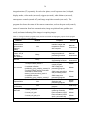
1. USB4000 Miniature Fiber Optic Spectrometer Optical Layout Explanation
(USB4000 Installation and Operation Manual) ..................................................33
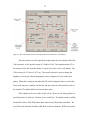
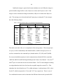
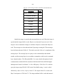
2. Listing of software programs used, routines used within each program,
purpose for the program and routine, and source of the software ......................34
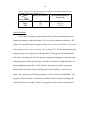
3. Values used to calculate reflectance for each of the color planes during the
2007 experiment with the photographic grey card .............................................43
4. Serial settings needed to communicate with the MS3100 imager ......................47
5. Message format to query or set the MS3100 integration time............................48
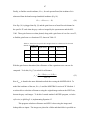
6. Values obtained in a test of the CCDs ability to quickly drain charge after
viewing bright conditions ...................................................................................61
7. Bleeding effect caused by CCD charge 'walk-off' (DN on a scale of 0-255) .....62
8. Change in reflectance of spectralon due to illumination angle (measured
from the surface normal) for 99% and 60% panels (Labsphere, Inc., 2006)......65
9. Reflectance values needed for the 50% reflectance panel to obtain 99% ±
4% reflectance for the 99% panel .......................................................................66
10. The percent reflectance for both spectralon panels, as specified by the
Labsphere data sheet. These values are spectrally integrated across the
specified bands (Labsphere, Inc., 2006) .............................................................66
11. Reflectance of, supposedly 18%, grey card for each spectral band imaged by
the MS3100.........................................................................................................81
12. Gain factor for specific ITs and gain factors as a function of ITs for each
channel of the MS3100 .......................................................................................87
13. 2007 mown segment Date versus NDVI regression R2 and p-values.................98
14. 2007 mown segment Date versus NDVI regression p-values that distinguish
between vegetation regions.................................................................................98
15. 2007 un-mown segment Date versus NDVI regression R2 and p-values .........102
x
LIST OF TABLES - CONTINUED
Table
Page
16. 2007 un-mown segment Date versus NDVI regression p-values that
distinguish between vegetation regions ............................................................102
17. 2008 mown segment Date versus NDVI regression R2 and p-values...............105
18. 2008 mown segment Date versus NDVI regression p-values that distinguish
between vegetation regions...............................................................................105
19. 2008 un-mown segment Date versus NDVI regression R2 and p-values .........107
20. 2008 un-mown segment Date versus NDVI regression p-values that
distinguish between vegetation regions ............................................................107
21. Individual plants’ Date versus NDVI regression R2 and p-values....................109
22. Individual plants’ Date versus NDVI regression p-values that distinguish
between individual plants and the un-mown region 3 ......................................109
23. Percentage change in the NDVI immediately after two hail storms for the
2008 mown segment .........................................................................................121
A1.Values used to calculate reflectance for each of the color planes during the
2007 experiment with the photographic grey card ...........................................151
A2.Serial settings needed to communicate with the MS3100 imager ....................163
A3.Message format to query or set the MS3100 integration time..........................164
xi
LIST OF FIGURES
Figure
Page
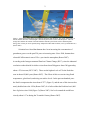
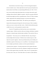
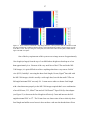
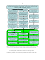
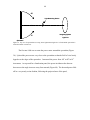
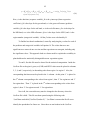
1. Earth surface/atmosphere solar radiation absorption and emission. The
yellow-orange lines on the left indicate that most of the sun light is absorbed
by the Earth’s surface and atmosphere. The red-orange lines indicate the
amount of thermal radiation emitted by the Earth’s surface and atmosphere
(Image adapted from Kiel and Trenberth, 1997, by Debbi McLean.) (Remer
2007) .....................................................................................................................2
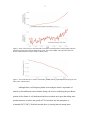
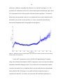
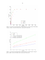
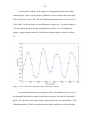
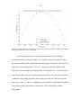
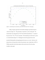
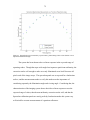
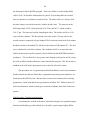
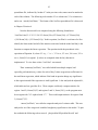
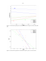
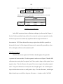
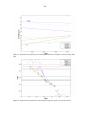
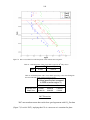
2. Plots of the increase in carbon dioxide concentration and temperature
(NASA graphs by Robert Simmon, based on carbon dioxide data from Dr.
Pieter Tans, NOAA/ESRL and temperature data from NASA Goddard
Institute for Space Studies.) (Remer 2007)...........................................................3
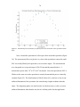
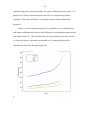
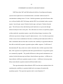
3. Plot of the decrease in volume of all Earth’s glaciers. (Glacier graph adapted
from Dyurgerov and Meier, 2005.) (Remer 2007) ...............................................3
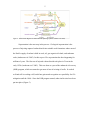
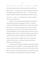
4. Basic block diagram of carbon dioxide capturing systems (Allam et al. 108) .....5
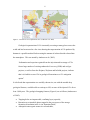
5. Location of CO2 sequestration sites (Anderson et al. 198) ..................................6
6. Basic block diagram of carbon dioxide capturing systems (Anderson et al.
199) .......................................................................................................................7
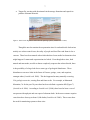
7. Vegetation kill at Mammoth Mountain, CA (http://pubs.usgs.gov/fs/fs17296/fs172-96.pdf)....................................................................................................8
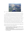
8. Arial View of ZERT Site ( Dobeck, Chem. Dept., MSU 2007) ...........................9
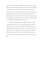
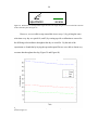
9. Spectrum of a healthy (gold), unhealthy (blue), and dead (grey) plants.
Spectrum acquired with a USB4000 spectrometer made by Ocean Optics,
Inc. ......................................................................................................................12
10. Vegetation Test Strip for 2007 (Shaw, ECE Dept., MSU 2007) ........................17
11. Vegetation Test Strip for 2008 (Shaw, ECE Dept., MSU 2008) ........................17
12. Spectral Absorption and Reflection Characteristics of Plants
(http://landsat.usgs.gov)......................................................................................20
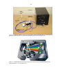
13. Imaging system including the MS-3100 three-CCD Imager made by
Geospatial Systems, Inc. and the small computer to run the system ..................24
xii
LIST OF FIGURES - CONTINUED
Figure
Page
14. Schematic optical layout of the MS-3100 with color-infrared setup
(www.geospatialsystems.com). ..........................................................................24
15. Transmittance of MS3100 channels in Color-IR mode. Green represents
green, red represents red, and dark red represents NIR
(www.geospatialsystems.com) ..........................................................................24
16. Zemax model of a MS3100 3-chip multispectral imager. Here green
represents the green color plane, blue represents the red color plane, and red
represents the NIR color plane, showing that the dichroic syrfaces are
modeled correctly................................................................................................26
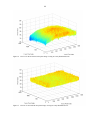
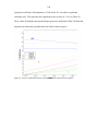
17. Power incident on modeled 3-chip imager detectors. These pictures show
the central beam and the edge-of-field beam, indicating that the optical
system simultaneously produces proper images on each of the three CCDs.
The top is the green color plane, the bottom left is the red color plane, and
the bottom right is the NIR color plane ..............................................................27
18. Camera Link High Speed Digital Data Transmission Cable
(http://www.siliconimaging.com/ARTICLES/CLink%20Cable.htm)................28
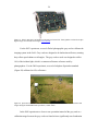
19. NI PCI-1428 base- and medium-configuration Camera Link frame grabber
card used to acquire digital images from the MS-3100 imager (www.ni.com)..29
20. Spectralon reflectance standard mounted on tripod for continuous
calibration of the MS-3100 imager during the 2008 ZERT field experiment
(J. Shaw 2008) ....................................................................................................29
21. Reflectance spectrum of photographic grey card used to calibrate the MS3100 imager during the 2007 ZERT field experiment........................................30
22. USB4000 Miniature Fiber Optic Spectrometer and Spectralon disk that were
used together to measure reflectance spectra of vegetation and calibration
panels (www.oceanoptics.com) ..........................................................................32
23. USB4000 Miniature Fiber Optic Spectrometer Optical Layout (USB4000
Installation and Operation Manual) ....................................................................32
24. DTControl Main Camera Control Panel (DTControl Software Users
Manual) ...............................................................................................................35
xiii
LIST OF FIGURES - CONTINUED
Figure
Page
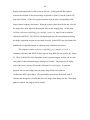
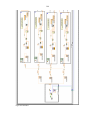
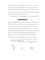
25. Flow diagram for ‘multiple extract planes.vi’, the image acquisition program
used in 2007 ........................................................................................................38
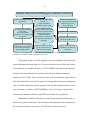
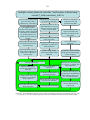
26. Flow diagram for ‘calculate reflection
(scaffolding_grey_multiple_scenes)2.vi’, the %reflectance and NDVI
calculation program used in 2007 .......................................................................41
27. Flow diagram for multiple extract planes & calculate %reflectance without
temp sensor(2_with correction)_test2.vi, the image acquisition, reflectance
and NDVI calculation program used in 2008 .....................................................44
28. A plot of the average digital number for each color plane as a function of
integration time. The full range of integration times, 1-130ms, is shown
here......................................................................................................................54
29. A plot of the average digital number for each color plane as a function of
integration time. The full working range of integration times, 1-20ms, is
shown here ..........................................................................................................55
30. A plot of the average digital number for each color plane as a function of
gain. The full range of gains, 2-36dB or 1.585-3981 on a linear scale, is
shown here in a linear scale ................................................................................56
31. A plot of the average digital number for each color plane as a function of
gain. A range of gains, 2-12dB or 1.585-15.85 on a linear scale, is shown
here in a linear scale............................................................................................56
32. A plot of average DN as a function of 1/(F/#)2 ...................................................57
33. Average DN, as measured by the imaging system, versus current measured
by the integrating sphere’s detector. ...................................................................58
34. A plot of the affect of temperature on the imager’s response.............................59
35. A plot of the affect of polarization angle on the imager’s response ...................60
36. 3-D view of uncorrected red color plane image viewing an evenly
illuminated scene ................................................................................................64
xiv
LIST OF FIGURES - CONTINUED
Figure
Page
37. 3-D view of corrected red color plane image viewing an evenly illuminated
scene....................................................................................................................64
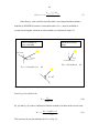
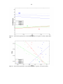
38. Top view for spectralon test setup, where light measuring device is rotated
around the spectralon ..........................................................................................67
39. Top view for spectralon test setup, where light measuring device is fixed
and the spectralon is rotated around it’s vertical axis .........................................68
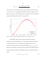
40. Normalized power measured by an optical power meter and cosine as a
function of viewing angle ...................................................................................69
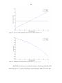
41. Normalized power measured by an optical power meter and cosine as a
function of the spectralon angle..........................................................................70
42. Normalized power measured by a spectrometer and cosine as a function of
viewing angle ......................................................................................................71
43. Normalized power measured by a spectrometer and cosine as a function of
the spectralon angle.............................................................................................72
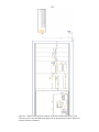
44. ZERT CO2 detection site layout .........................................................................73
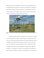
45. Imager orientation at the ZERT Site in 2007......................................................74
46. View of 2007 setup showing imager orientation in respect to the vegetation
test strip (Shaw, ECE Dept., MSU 2007) ...........................................................75
47. View of 2007 vegetation scene from scaffolding. Mown and Un-mown
regions 1, 2, and 3 shown here (Shaw, ECE Dept., MSU 2007) ........................76
48. View of 2007 vegetation scene. Mown and Un-mown regions 1, 2, and 3
are shown here (Shaw, ECE Dept., MSU 2007).................................................77
49. Imager orientation at the ZERT Site in 2008......................................................78
50. View of 2008 vegetation scene. Mown and un-mown regions 1, 2, and 3 are
shown here (Shaw, ECE Dept., MSU 2008).......................................................79
51. View of Plants 8, 9, 10 (Shaw, ECE Dept., MSU 2008). ...................................80
xv
LIST OF FIGURES - CONTINUED
Figure
Page
52. Reflectance for one day using grey card to calibrate all images.........................82
53. Imager and MODTRAN setup to equate horizontal and vertical irradiances.....84
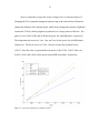
54. Irradiance modeled by MODTRAN and measured by a pyranometer for one
day.......................................................................................................................85
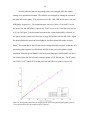
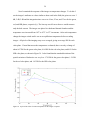
55. Polynomial fit for the MODTRAN-Pyranometer irradiance difference, Efit ......86
56. MODTRAN modeled irradiance polynomial fit, EMODTRAN,300-3000nm.................86
57. Erroneous reflectance data due to differences in sun-spectralon angle and
sun-scene angle ...................................................................................................89
58. Differences in sun-spectralon angle and sun-scene angle...................................90
59. Accurate reflectance data taken with spectralon laid flat ...................................90
60. Spectralon and vegetation scene viewed at the same angle to remove the
effect of a variable illumination angle on the calibration panel..........................91
61. 2007 mown segment green, red, and NIR reflectances for regions 1 (solid), 2
(dash), and 3 (dot) ...............................................................................................99
62. 2007 mown segment Date versus NDVI for regions 1 (green), 2 (red), and 3
(blue) ...................................................................................................................99
63. 2007 un-mown segment green, red, and NIR reflectances for regions 1
(solid), 2 (dash), and 3 (dot)..............................................................................101
64. 2007 un-mown segment Date versus NDVI for regions 1 (green), 2 (red),
and 3 (blue) .......................................................................................................101
65. 2008 mown segment green, red, and NIR reflectances for regions 1 (solid), 2
(dash), and 3 (dot) .............................................................................................104
66. 2008 mown segment Date versus NDVI for regions 1 (green), 2 (red), and 3
(blue) .................................................................................................................104
xvi
LIST OF FIGURES - CONTINUED
Figure
Page
67. 2008 un-mown segment green, red, and NIR reflectances for regions 1
(solid), 2 (dash), and 3 (dot)..............................................................................106
68. 2008 un-mown segment Date versus NDVI for regions 1 (green), 2 (red),
and 3 (blue) .......................................................................................................106
69. Green, red, and NIR reflectances for individual plants within un-mown
segment .............................................................................................................108
70. Date versus NDVI for individual plants within 2008 un-mown segment. .......109
71. 2007 CO2 flux map of the ZERT CO2 Detection site (adapted from J.
Lewicki, Lawrence Berkeley National Laboratory 2007) ................................110
72. 2008 CO2 flux map of the ZERT CO2 Detection site (adapted from J.
Lewicki, Lawrence Berkeley National Laboratory 2008) ................................114
73. Position and number of soil moisture probes (adapted from L. Dobeck,
Chem. Dept., MSU 2008) .................................................................................115
74. Soil moisture for mown strip probes (adapted from L. Dobeck, Chem. Dept.,
MSU 2008)........................................................................................................115
75. Soil moisture for un-mown strip probes (adapted from L. Dobeck, Chem.
Dept., MSU 2008).............................................................................................116
76. Precipitation data (adapted from J. Lewicki, Lawrence Berkeley National
Laboratory 2008) ..............................................................................................116
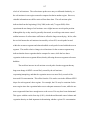
77. Image of mown and un-mown segments taken 9 July 2008 (a) and 9 August
2008 to visually illustrate the change in the health of the vegetation (J. Shaw
2008) .................................................................................................................118
78. Close up images of mown segment taken 9 July 2008 (a) and 9 August 2008
(b) to visually illustrate the change in the health of the vegetation (J. Shaw
2008) .................................................................................................................118
xvii
LIST OF FIGURES - CONTINUED
Figure
Page
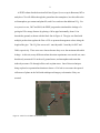
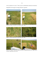
79. Images taken 3 July 2008 (a) and 9 August 2008 (b) to visually illustrate the
change in the health of the vegetation (J. Shaw 2008). Plant 10’s location is
indicated by the blue circle. Plants 8 and 9’ locations are indicated by the
red circle............................................................................................................119
A1.Flow diagram for ‘multiple extract planes.vi’, the image acquisition program
used in 2007 ......................................................................................................137
A2.‘multiple extract planes.vi’ the LabVIEW block diagram for the program
used to acquire images in 2007.........................................................................138
A3.Flow diagram for ‘calculate reflection
(scaffolding_grey_multiple_scenes)2.vi’, the %reflectance and NDVI
calculation program used in 2007 .....................................................................145
A4.‘calculate reflection (scaffolding_grey_multiple_scenes)2.vi’ the LabVIEW
block diagram for the program used calculate reflectance and NDVI in
2007...................................................................................................................146
A5.Flow diagram for multiple extract planes & calculate %reflectance without
temp sensor(2_with correction)_test2.vi, the image acquisition, reflectance
and NDVI calculation program for 2008 ..........................................................152
A6.Flow diagram for multiple extract planes & calculate %reflectance without
temp sensor(2_with correction)_test2.vi, the image acquisition, reflectance
and NDVI calculation program used in 2008 ...................................................153
xviii
ABSTRACT
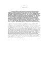
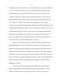
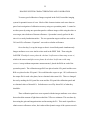
In response to the increasing atmospheric concentration of greenhouse gasses,
such as CO2 produced by burning fossil fuels, which is very likely linked to climate
change, the Zero Emissions Research Technology (ZERT) program has been researching
the viability of underground sequestration of CO2. This group’s research ranges from
modeling underground sequestration wells to detection of leaks at test sites. One of these
test sites is located just west of Montana State University in Bozeman, MT, at 45.66°N
111.08°W. At this site experiments were conducted to assess the viability of using
multispectral imaging to detect plant stress as a surrogate for detecting a CO2 leak. A
Geospatial Systems MS3100 multispectral imager, implemented in color-infrared mode,
was used to image the plants in three spectral bands. Radiometric calibration of the
output of the imager, a digital number (DN), to a reflectance was achieved using a grey
card and spectralon reflectance panels. To analyze plant stress we used time series
comparisons of the bands and the Normalized Difference Vegetation Index (NDVI),
computed from the red and near-infrared band reflectances. Results were compared with
rainfall, soil moisture, and CO2 flux data. The experiment was repeated two years in a
row; the first from June 21, 2007 to August 1, 2007 and the second from June 16, 2008 to
August 22, 2008. Data from the first experiment showed that plants directly over the leak
were negatively affected quickly, while plants far from the pipe were affected positively.
Data from the second experiment showed that the net effect of leaking CO2 depends on
the relationship between CO2 sink-source balance and vegetation density. Also, due to
the strong calibration techniques employed in 2008, the imaging system was able to see
the effects of water and hail on the vegetation. We have also found a way to image
continuously through the day, not having to worry about clouds or sun-to-scene/scene-toimager angle effects. This system’s easy setup, automation, all-day imaging capability,
and possibility for low cost makes it a very practical tool for plant stress measurements
for the purpose of detecting leaking CO2.
1
INTRODUCTION
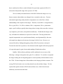
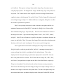
Greenhouse gases make life sustainable on Earth by trapping some of the Sun’s
incoming short wave radiation in an Earth surface-atmosphere energy transfer system, the
greenhouse effect. The warming of the Earth starts with short wave radiation entering the
atmosphere. About 30% of this radiation is reflected back into space by clouds,
atmospheric particles, reflective ground surfaces, and the ocean surf, so about 70% of the
short wave solar radiation is absorbed by land, air, and ocean (Remer 2007). These Earth
features then emit this energy as long wave thermal radiation. Almost half of this
reemitted radiation is transmitted out of the atmosphere and more than half is absorbed by
greenhouse gases such as carbon dioxide (CO2), water vapor (H2O), and methane (CH4).
The energy absorbed by the greenhouse gases is then re-emitted, with some going back to
the Earth surface to create a continual chain of energy transport between the Earth and
the clouds or gases. This is a good thing, though, because without the greenhouse effect
the Earth’s average equilibrium temperature would be about -18oC instead of 15oC
(Remer 2007). However, more greenhouse gases in the atmosphere will lead to greater
heat retaining capacity and higher equilibrium temperature.
2
Figure 1: Earth surface/atmosphere solar radiation absorption and emission. The yellow-orange lines on
the left indicate that most of the Sunlight is absorbed by the Earth’s surface and atmosphere. The redorange lines indicate the amount of thermal radiation emitted by the Earth’s surface and atmosphere.
Energy flux in watts per meter squared (Image adapted from Kiel and Trenberth, 1997, by Debbi McLean.)
(Remer 2007)
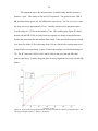
Scientists have found that humans have been increasing the concentration of
greenhouse gases over the past 250 years at increasing rates. Since 2004, humans have
released 8 billion metric tons of CO2 a year into the atmosphere (Remer 2007).
According to the Intergovernmental Panel on Climate Change (IPCC), since the industrial
revolution carbon dioxide levels have risen from about 280 ppm to about 380 ppm today,
about a 35% increase (IPCC 2007). These are the highest levels of CO2 the Earth has
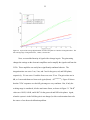
seen in about 650,000 years (Remer 2007). The effects of this are seen in rising Earth
temperatures, glacial melt, and rising sea surface levels. In the past one hundred years
the Earth’s temperature has risen about 0.75oC (Figure 2), and the rate of this increase has
nearly doubled since the 1950s (Remer 2007). It is believed that the Earth has lost 8,000
km3 of glaciers since 1960 (Figure 3) (Remer 2007). Sea levels around the world have
risen by about 0.17 m during the Twentieth Century (Remer 2007).
3
Figure 2: Plots of the increase in carbon dioxide concentration and temperature (NASA graphs by Robert
Simmon, based on carbon dioxide data from Dr. Pieter Tans, NOAA/ESRL and temperature data from
NASA Goddard Institute for Space Studies.) (Remer 2007).
Figure 3: Plot of the decrease in volume of all Earth’s glaciers (Glacier graph adapted from Dyurgerov and
Meier, 2005.) (Remer 2007)
Although there is still lingering debate concerning the relative importance of
natural cycles and human-caused climate change, the science underlying the greenhouse
portion of the climate is well understood and most scientists now agree that taking some
prudent measures to reduce the growth of CO2 emissions into the atmosphere is
warranted (IPCC 2007). With this in mind, there is growing interest among many
4
organizations to do something to mitigate emission of greenhouse gases in the attempt to
reduce or stop contributing to the warming of the Earth. At this point in time most of our
energy production comes from fossil fuels, which create carbon dioxide when burned.
Therefore, it is doubtful that humans can simply stop using fossil fuels as a source of
energy in the near future. However, one option being explored at this time is the capture
and geological sequestration of carbon dioxide.
The capture of carbon dioxide is being explored mostly for large-scale fossil fuel
power plants, fuel processing plants and other industrial plants (Allam et al. 2005).
Small-scale capture at this point would be too difficult and expensive (for example,
applied to individual cars). To mitigate these small sources, an energy carrier, such as
hydrogen or electricity, could be produced at fossil fuel plants with capture technologies
(Allam et al. 2005). The capture process basically emits non-greenhouse gases, such as
O2 and N2, and compresses and dehydrates the carbon dioxide for easy shipment and
sequestration (Figure 4). The four basic types of capture systems are as follows (Allam et
al. 2005):
• Capture from industrial process streams;
• Post-combustion capture;
• Oxy-fuel combustion capture;
• Pre-combustion capture.
5
Figure 4: Basic block diagram of carbon dioxide capturing systems. (Allam et al. 2005)
Sequestration is the next step in the process. Geological sequestration is the
process of injecting captured carbon dioxide into suitable rock formations where most of
the Earth’s supply of carbon is held in coals, oil, gas-organic-rich shale, and carbonate
rocks (Anderson et al. 2005). In this respect CO2 sequestration has been happening for
millions of years. The first test of injected carbon dioxide took place in Texas in the
early 1970s (Anderson et al. 2005). This was done as a part of the enhanced oil recovery
(EOR) program, which was started to get more oil out of existing oil wells. It worked
well and still is working well, but did not gain much recognition as a possibility for CO2
mitigation until the 1990s. Since the EOR program started, other similar sites have been
put into place (Figure 5).
6
Figure 5: Location of CO2 sequestration sites. (Anderson et al. 2005)
Geological sequestration of CO2 is naturally occurring at many places across the
world and has been tested at a few sites showing that sequestration of CO2 produced by
humans is a possible method for decreasing the amount of carbon dioxide released into
the atmosphere. This was stated by Anderson et al. (2005):
“Information and experience gained from the injection and/or storage of CO2
from a large number of existing enhanced oil recovery (EOR) and acid gas
projects, as well as from the Sleipner, Weyburn and In Salah projects, indicate
that it is feasible to store CO2 in geological formations as a CO2 mitigation
option.”
It is believed that sequestration at a carefully chosen site, one with the needed deep
geological features, would be able to retain up to 99% or more of the injected CO2 for at
least 1,000 years. The geological trapping features (Figure 6) are as follows (Anderson et
al. 2005):
•
•
•
Trapping below an impermeable, confining layer (caprock);
Retention as an immobile phase trapped in the pore spaces of the storage
formation; dissolution in the in situ formation fluids;
Adsorption onto organic matter in coal and shale;
7
•
Trapped by reacting with the minerals in the storage formation and caprock to
produce carbonate minerals.
Figure 6: Basic block diagram of carbon dioxide capturing systems (Anderson et al. 2005).
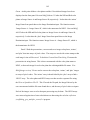
Though the need to monitor the sequestration sites for carbon dioxide leaks arises
mainly as a carbon control issue, the safety of people and local flora and fauna is also a
concern. There have been natural carbon leaks that have been studied to determine what
might happen if a man-made sequestration site leaked. Even though these sites, both
natural and man-made, are able to almost completely sequester the carbon dioxide, there
is the possibility of a large leak due to some type of geological disturbance. These
disturbances can cause leaks in the forms of fissures, springs, vents, and eruptions,
amongst others (Lewicki et al. 2006). This has happened at many naturally occurring
CO2 geologic reservoirs, causing flora and fauna to die. For example, at Mammoth
Mountain, CA for the past 30 years there has been a definite vegetation kill (Figure 7)
(Lewicki et al. 2006). According to Lewicki et al. (2006), there has also been a case of
one person with asphyxia and one report of a human death. In the more extreme eruption
cases there have been up to about 1,800 deaths (Lewicki et al. 2006). These cases show
the need for monitoring systems at these sites.
8
Figure 7: Vegetation kill at Mammoth Mountain, CA. (http://pubs.usgs.gov/fs/fs172-96/fs172-96.pdf)
In 2005 a large group of researchers came together and started a research group
focused on developing the monitoring technologies that are required to move forward
with practical carbon sequestration. This Zero Emissions Research and Technology
(ZERT) program is a research group dedicated to investigating the viability, safety, and
reliability of geological sequestration of carbon dioxide via leak detection. “ZERT is a
partnership involving DOE laboratories (Los Alamos National Laboratory, Lawrence
Berkeley National Laboratory, National Energy Technology Laboratory, Lawrence
Livermore National Laboratory, and Pacific Northwest National Laboratory) as well as
universities (Montana State University and West Virginia University)” (Spangler 2005).
The ZERT research goals are as follows (Spangler 2005):
•
•
•
•
Development of sophisticated, comprehensive computer modeling suites which
predict the underground behavior of carbon dioxide
Investigation of the fundamental geochemical and hydrological issues related to
underground carbon dioxide storage
Development of measurement techniques to verify storage and investigate leakage
Development of mitigation techniques and determination of best practices for
reservoir management
9
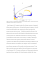
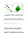
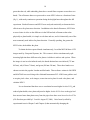
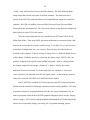
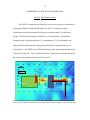
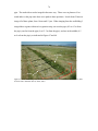
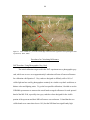
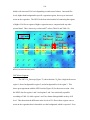
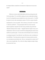
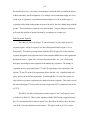
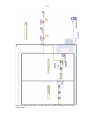
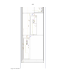
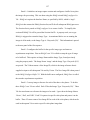
A ZERT carbon dioxide detection field site (Figure 8) was set up in Bozeman, MT to
study how CO2 will diffuse through the ground into the atmosphere, how this affects the
soil/atmosphere gas content and plant life, and if we can detect the additional CO2. For
two years in a row, 2007 and 2008, the ZERT program has simulated the leakage of a
geological CO2 storage features by placing a 100 m pipe horizontally, about 1.8 m
beneath the ground, as shown with the black line in Figure 8. The pipe was fitted with
multiple packers that regulate the flow of CO2 to promote homogenous release along the
length of the pipe. The CO2 flow rate was 0.1 tons/day and 0.3 tons/day for 2007 and
2008, respectively. These rates were chosen because they cover the maximum allowable
leakage. At this site, many different carbon detection experiments were carried out, some
that directly measured CO2 in the soil, ground water, and atmosphere and some that
indirectly measure CO2 through effects such as plant stress. One of these techniques
being explored as a potential mechanism to detect a CO2 leak is to measure the spectral
reflectance of plants in the field with multispectral imagery to determine if they are
stressed.
NE
end
Pipe
SW
end
Figure 8: Arial View of ZERT Site (Dobeck 2008).
Power Post
10
Researchers have used remote sensing as a tool for detecting plants and plant
stress for a number of years. Remote plant detection took a big step towards plant stress
detection when Color-IR film was invented during WWII (Paine et al. 2003). The US
Army was not actually trying to detect plants; they were trying to detect tanks, people,
and things of that sort that were hidden in vegetation. After the war people realized that
this film format might be useful for vegetation detection. Then in 1972 the first Landsat
satellite, implemented with a multispectral imager, was put into orbit explicitly to
monitor Earth’s landmasses (Rocchio 2008). Since then many more multispectral
imagers and some hyperspectral imagers have been sent into space, flown on airplanes,
and set up on towers to analyze the Earth’s surface. With all of this detailed image data
available, there arose a need to quantitatively analyze the data.
Since the 1970s significant work has been done to more accurately analyze
vegetation imagery. Initially, researchers with years of training would analyze vegetation
imagery by viewing the images, band-by-band or multiband. This worked well, but was
not quantitative. The next step was to use calibrated reflectances, the percentage of
incident sunlight reflected by objects. With these data, researchers began to see that
objects have spectral ‘signatures,’ and more specifically that the spectra of healthy and
non-healthy vegetation of the same type were very different. So by analyzing the relative
levels of multiple spectral bands, researchers were able to glean information on
vegetation spectral ‘signatures.’ Knowing what portions of the vegetation reflectance
spectra are most affected by stress led to the combination of multiple spectral bands into
what are called vegetation indices (Jensen 2000). Many, at least 30, vegetation indices
have been used over the years. Each of these indices was created to examine different
11
characteristics of plant health by analyzing different parts of the reflectance spectrum.
Some look at overall plant health, some look at water content, some look at chlorophyll
content, and there are many others. Realizing that each of these indices measures
somewhat specific characteristics of plant health, researchers have been trying to model
biophysical parameters, such as leaf area index, total biomass, and gross CO2 flux
estimation (de Jesus et al. 2001; Nakaji et al. 2007). This thesis describes experimental
research conducted to assess the potential utility of a platform-based multispectral imager
for detecting leaking CO2 through plant stress measurements.
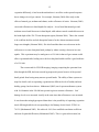
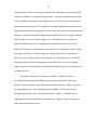
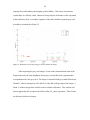
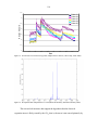
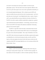
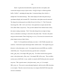
Many remote sensing techniques for detecting plants or plant stress exploit a
spectral signature called the “red edge.” The red edge is the steep rise in vegetation
reflectance that occurs near 700 nm, with an inflection point connecting the low red
reflectance and high near-infrared (NIR) reflectance. As vegetation is stressed, the red
edge shifts to shorter wavelengths and becomes less steep (Figure 9). In Figure 9, the
gold line is a reflectance spectrum measured for a healthy plant, the blue line is the
reflectance spectrum of an unhealthy plant, and the gray line is the spectrum of a dead
plant.
12
Inflection
Point
Figure 9: Spectrum of a healthy (gold), unhealthy (blue), and dead (grey) plants. Spectrum acquired with a
USB4000 spectrometer made by Ocean Optics, Inc.
Carter (Responses 1993) completed a study of the reflectance spectrum of vegetation of
different species to different stresses. He hoped to define spectral ‘signatures’ of specific
stresses that could be applied to any vegetation and to define what regions of the
spectrum are most sensitive to stresses. To do this he measured the reflectances of six
plant species that were stressed by four biological and four physiochemical stress agents
(Carter, Responses 1993). Reflectance measurements were made using a scanning
spectroradiometer with 768 channels. Stress sensitivity was found by subtracting the
reflectance of non-stressed vegetation (control) from the reflectance of stressed
vegetation for each channel of the spectroradiometer, then dividing this difference by the
non-stressed reflectance at each channel (Carter, Responses 1993). He found that the
green reflectance spectrum near 550 nm and the red reflectance spectrum near 710 nm
both increased the same amount, regardless of the specific plant species or stress agent
(Carter, Responses 1993). The increase in reflectance near 700 nm agreed with previous
data (Horler, Dockray, and Barber 1983; Rock, Hoshizaki, and Miller 1988; Curran,
13
Dungan, and Gholz 1990; Cibula and Carter 1992), in that the red edge shifts towards
shorter wavelengths when a plant is stressed. Carter (Responses 1993) states that there
are maxima of the vegetation reflectance sensitivity to stress in the 535-640 nm and 685700 nm regions of the spectrum.
In a later work by Carter et al. (Leaf 2001), he found that the 700 nm region was
the most sensitive to stresses due to the loss of chlorophyll and the absorption
characteristics of chlorophyll. More specifically Carter et al. (Leaf 2001) comments that
far-red reflectance will increase considerably if chlorophyll levels decrease slightly. He
also noted that in the near-infrared, a change in reflectance would only be expected to
result from a change in leaf anatomy or water content, not chlorophyll levels (Carter et al.
Leaf 2001). He summed things up by stating that specific stress agents do not have
spectral ‘signatures.’ So one should be able to detect changes in chlorophyll
concentrations, leaf anatomy, and water content by analyzing both the red and NIR
portions of the spectrum, or by analyzing an index that combines these bands (Jordan
1969; Carter et al. Leaf 2001).
One such index that lends itself to vegetation remote sensing measurements is the
Normalized Difference Vegetation Index (Rouse et al. 1974), or NDVI, defined as
NDVI =
ρ NIR − ρ RED
.
ρ NIR + ρ RED
(1)
In this equation, ρNIR is the reflectance of a scene in the NIR portion of the spectrum and
ρRED is the reflectance of a scene in the red portion of the spectrum. Considering Carter’s
work, an index like NDVI should be useful for detecting plant stress. Gamon et al.
(1999) noted that NDVI is a good marker for canopy structure, chlorophyll content,
nitrogen content, fractional intercepted or absorbed photosynthetically active radiation,
14
and potential photosynthetic activity across many different types of vegetation. Nakaji et
al. (2007) also found a correlation of 0.82 between NDVI and fractional intercepted
photosynthetically active radiation in numerous vegetation types irrespective of sky
conditions, leading him to construct a linear regression equation to calculate absorbed
photosynthetically active radiation with a root-mean-square error (RMSE) of less than
10%. Fuentes et al. (2007) did an experiment measuring the CO2 flux via eddy
covariance towers and compared the results to NDVI trends calculated for that area. They
found that NDVI had a high correlation, -0.981, with carbon flux (Fuentes et al. 2007). It
was determined that NDVI was able to capture the effects of changing environmental
conditions, such as drought, recovery, and then fire on the carbon flux (Fuentes et al.
2007). According to this, it is reasonable to believe that NDVI could see the effects of
rain, hail, and small amounts of carbon dioxide on vegetation.
Maynard et al. (2006) did a study on the ability of indices as compared to nontransformed bands to accurately model biophysical parameters. She compared linear
regression models that estimate TTB (total transformed biomass) using NDVI and nontransformed bands (bands 4 and 7 of Landsat) as the predictors. The regression models
were built using extra sums-of-squares F-tests (Lawrence et al. 1998) and R2 values were
used to determine the variability in biomass (Maynard et al. 2006). NDVI explained 41%
of the variability while the non-transformed bands explained 53% of the variability
(Maynard et al. 2006).
I am not aware of any publications dealing with the effects of added carbon
dioxide to plant health, but there might be similar affects from other gases. Though
carbon is a fertilizer in some cases and different gases will affect the spectrum of
15
vegetation differently, it has been shown that there is an effect on the spectral response
due to changes in soil gas content. For example, Noomen (2006) did a study on the
effects of natural gas, methane and ethane, on the reflectance of maize. Noomen (2006)
converted reflectances to band depths for analysis. It was found that natural gas and
methane caused small decreases in band depth, while ethane caused a marked decrease in
the band depth of the 550-750 nm absorption region (Noomen 2006). There also seemed
to be a shift in the blue and red absorption features for the ethane treatment towards
longer wavelengths (Noomen 2006). She also found that there was a decrease in the
reflectance at a water absorption band, perhaps by ethane causing a decrease in water
uptake. This experiment may be analogous to a CO2 leak in that soil gas content would
affect vegetation health, leading one to believe that plant health could be a good indicator
of a CO2 leak.
The recent trend for VIS-NIR imaging, imaging comprising the spectrum from
blue through the NIR, has been towards hyperspectral systems because of the spectral
detail gained from having many narrow spectral bands. The ability of these systems to
map fine details, such as separating vegetation into different levels of healthy and nonhealthy groups, has been shown. Muhammed (2002) used a spectroradiometer system
with 164 channels in the 360-900 nm spectral region to measure reflectance. Leaf
damage levels were measured visually at the same time that reflectances were measured.
It was shown that using hyperspectral data there is the possibility of separating vegetation
into 8 differing health levels corresponding to leaf damage levels from 0.59798% to
76.15% (Mohammed 2002). He achieved ~94% for a modified correlation coefficient
and sum of squared differences (Mohammed 2002). This is a great achievement, but
16
dealing with the overwhelming amount of data inherent and cost associated with this type
of system can be bothersome, especially when a multispectral system may be able to
delineate between stressed and non-stressed plants sufficiently well with only a few
spectral points.
Seeing the need for CO2 leak detection and potential ability of multispectral
imagers to detect plant stress due to a CO2 leak, I measured the spectral response of plants
at the ZERT CO2 detection site and analyzed single bands and NDVI in a temporal
fashion. During 2007 and 2008, the ZERT CO2 detection experiment was held in a field
just west of Montana State University in Bozeman, MT. Multispectral imaging data were
collected during both experiments.
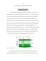
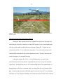
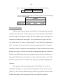
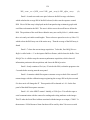
In 2007, a 100m vegetation test strip was set orthogonally to the center of the
carbon dioxide release pipe, with half the strip mowed and the other half left un-mown
(Figure 10). The multispectral imager viewed the vegetation to about 10 m past the pipe
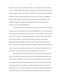
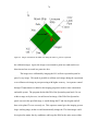
on the northwest side. In 2008 there was a 30×20m vegetation area set up for vegetation
testing (Figure 11). Out of this vegetation area we imaged a 4×11m section. Both years I
imaged a mown and an un-mown section. The intent was to use northwest edge furthest
from the imager as a control with little to no influence from the leaking CO2, and the
section nearest the pipe as the primary test area. During the 2008 test we also imaged
three specific plants on the outer edge of the un-mown strip, just on the northwest side of
the pipe, to overlap with data acquired by another researcher using a hyperspectral
system.
17
Figure 10: Vegetation Test Strip for 2007.
Figure 11: Vegetation Test Strip for 2008.
The first CO2 injection took place from July 9, 2007 to July 23, 2007. Images
were acquired from June 21, 2007 to August 1, 2007, though 15 days were skipped
because of scattered cloud coverage that prevented the imager from achieving reliable
calibration. The second CO2 injection took place from July 7, 2008 to August 7, 2008.
Images were acquired from June 16, 2008 to August 22, 2008. Cloud coverage was not a
problem in 2008 since the system was implemented with automated exposure control and
calibration panel auto-referencing for every image. Images of background conditions
were acquired before and after the CO2 injections ended each year.
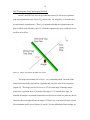
The imaging system I designed was mounted on a small tower with a -45o
viewing angle, so that it viewed the ground directly above the buried release pipe out to
about 10 meters away from the pipe. The system makes calibrated reflectance
measurements of three spectral bands in the near-infrared, red, and green, using a
Spectralon calibration target as a Lambertian reference. These three bands were chosen
since it is known that healthy plants are highly reflective in the near infrared, while
unhealthy plants are not. In addition, healthy plants usually have higher reflectance in the
18
green than the red, while unhealthy plants have a much flatter response across these two
bands. The reflectance data were processed to create NDVI values as a function of time
(Eq. 1), with nearly continuous operation during the daylight hours throughout the full
experiment. Both reflectances and NDVI were analyzed statistically to determine their
effectiveness for plant stress detection. In addition to the band reflectances, NDVI also
was used since it relies on the difference in the NIR and red reflectances that relate
physically to plant health, it is simple to calculate and use, and it is historically one of the
most commonly used indices for plant detection. Generally speaking, the greater the
NDVI value, the healthier the plant.
To obtain the three spectral bands simultaneously, I used the MS3100 three-CCD
imager made by Geospatial Systems, Inc. This camera is able to simultaneously split
incoming light into three different color planes via dichroic surfaces and a prism. When
the imager is run in color-infrared mode, the bands obtained are near-infrared (735 nm865 nm), red (630 nm-710 nm), and green (500 nm-580 nm). These three bands were
chosen to mimic the popular Landsat satellite bands. Then software written in LabVIEW
and MATLAB was used along with a National Instruments PCI-1428 Frame grabber card
to acquire pixel values, scale images, create time-series plots for each color plane, and
calculate NDVI.
It was determined that there was a correlation between higher levels of CO2 and
reduced plant health, since plants subjected to higher levels of CO2 close to the pipe had
been stressed more than plants away from the pipe where there were lower levels of CO2
(CO2 flux data provided by J. Lewicki August 25, 2008). I also found (verified by
experimental tests in Chapter 3 and Chapter 4) that automatically changing the
19
integration time and auto-referencing a stationary spectralon panel greatly increased the
accuracy and stability of reflectance measurements. This improved calibration provided
greater confidence in the data, even making it possible to see the effects of rain and hail
and nourishments and stresses. The multispectral imaging approach demonstrated in this
experiment therefore offers potentially lower cost, does not require as much operator time
and effort, can image continually throughout daylight hours in clear or cloudy conditions,
and can image over a wide range of angles. It was unfortunate that our system was
pointed such that the field of view happened to almost entirely miss one of several
isolated CO2 ‘hotspots’ that happened to occur in only a few small areas of the test field.
The imager was able to see just the edge of one hotspot, which gave us the chance to
show the system’s ability to detect small amounts of elevated plant stress. Overall, the
data gained from this experiment demonstrate the effectiveness of a tower-mounted
multispectral imager for detecting an underground carbon dioxide leak via plant stress on
a continuous basis.
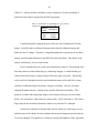
The balance of this thesis is organized as follows. Chapter 2 presents a
description of the multispectral imaging system developed and used for this study.
Chapter 3 discusses imager system characterization and calibration. Chapter 4 presents
the experimental setup of the imaging system at the ZERT CO2 detection site and
imaging methods for the 2007 and 2008 experiments. Chapter 5 communicates the
experimental results and a discussion of implications. Chapter 6 wraps everything up
with conclusions and future work.
20
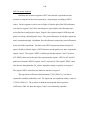
MULTISPECTRAL VEGETATION IMAGING
Spectral Response of Plants
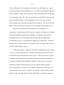
It is possible to detect plant stress by inspecting the plant’s spectral response
pattern temporally. The absorption and reflectance characteristics of a plant come about
because of the interaction of light with the constituents of plants, such as chlorophyll,
mesophyll, cell structure, and water content. The plant pigments that dominate the
reflectance spectrum are the chlorophyll inside the collenchyma that reflects green light
and the spongy parenchyma in the mesophyll that reflects near infrared (NIR) radiation
(USGS 2008). Blue and red light are absorbed by the chlorophyll and then used for
energy production in photosynthesis (Figure 12). Consequently, healthy plants are highly
reflective in the near infrared, while unhealthy plants are less so. In addition, healthy
plants are more reflective in the green than in the red and blue, while unhealthy plants
have higher and flatter reflectance throughout each of these bands (Figure 9).
Figure 12: Spectral Absorption and Reflection Characteristics of Plants (http://landsat.usgs.gov).
By analyzing the reflectance of each band used in the MS3100 multispectral
imager (green 500-580 nm, red 630-710 nm, and NIR 735-865 nm) temporally, one is
21
able monitor the temporal evolution of plant stress. When a plant becomes stressed we
expect to see the NIR band reflectance decrease and the green and red band reflectances
increase leading to a flatter total spectrum. This leads to a decrease in both the red-NIR
reflectance difference and the normally steep slope of the red edge, corresponding to a
blue shift of the inflection point (Carter 2001) between the red and NIR bands. The
Normalized Difference Vegetation Index (NDVI) (Eq.1) takes advantage of this
difference between the red and NIR bands.
We expect changes in the spectrum of the vegetation to come about from changes
in long-term environmental factors, such as the soil/atmospheric CO2 levels, analogous to
work done by Noomen (2006), seasonal water levels, and seasonal heat. It is possible for
excess CO2 to be helpful or harmful, depending on the CO2 sink-source balance and the
density of the vegetation. Arp (1991) showed that even though CO2 stimulates
photosynthesis, long-term high levels of CO2 could cause photosynthetic capacity to
decrease when there is a source-sink imbalance and dense plant growth. This in turn will
lead to a decrease in chlorophyll content (Arp 1991). Conversely, Kimball et al. (1993)
states when CO2 levels are doubled, plant growth and yield increase by 30%.
This all suggests that, depending on how close the plants are to the leak and the
level of CO2 that they are exposed to: there may be some plants that feel negative stress
and some that are nourished. Of course, if it is hot and dry plants will dry up, wilt and
die, leading to a decrease in chlorophyll and water content. Conversely, increased CO2
can decrease plant water content loss by stomatal regulation, thereby increasing leaf
thickness (Arp 1991). No matter what the stress agent, with a change in chlorophyll and
water content there will be a notable change in the reflectance spectrum of vegetation.
22
Vegetation reflectance is also altered by short-term diurnal effects of temperature,
humidity, and light levels on photosynthetic rate and plant respiration. Huck et al. (1962)
notes that root respiratory rates were 25-50% higher during the daylight hours than at
night, when temperature and humidity were held constant. Also, leaf respiratory rates
grow exponentially due to short-term temperature increase, and at the same temperature
respiratory rates are greater in the afternoon than in the morning with the same levels of
irradiance (Atkin et al. 2000). This will lead to the plant drying out throughout the day,
causing it to look somewhat stressed in the afternoon compared to the morning. Raschke
(1985) notes that decreasing humidity while holding temperature and irradiance constant
throughout the day will decrease the photosynthetic rate, especially when there are dry
soil conditions, thereby decreasing chlorophyll levels.
On the contrary, it has been found that greater irradiance leads to a greater
photosynthetic rate (Kalt-Torres et al. 1987). This will increase absorption of red
wavelengths, thereby increasing NDVI, making the plants look healthier. It is hard to say
if the photosynthetic rate will increase or decrease on a whole. Considering
environmental factors and diurnal variations, the CO2 flux, water level, temperature, and
rain data collected by my colleagues and myself are very important to understand what
we are seeing in terms of plant stress.
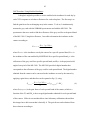
To detect plant stress, due to a CO2 leak, I designed a system consisting of a 3color CCD imager mounted on a scaffold, operated by a small computer automatically in
the field, and calibrated by a photographic grey card or spectralon panel. The imager
collects green, red, and NIR portions of the spectrum, separately, for a vegetation scene
and the calibration target, simultaneously. This data is then used by the computer to
23
calculate reflectances for each band and NDVI. The system computes reflectances and
NDVI for two vegetation segments, mown and un-mown vegetation, split into three
sections each, one near the pipe, one far from the pipe and one in the middle. Then the
reflectances and NDVI are plotted so the time evolution of the reflectance and NDVI
could be analyzed.
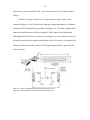
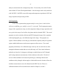
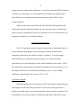
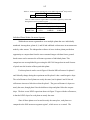
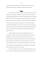
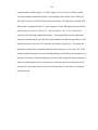
Imaging Hardware
We have developed and deployed a multispectral imaging system to detect plant
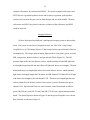
stress. The system is based on a Geospatial Systems, Inc. MS-3100 3-chip ChargeCoupled Device (CCD) imager (Figure 13) that images in three spectral bands of interest
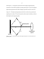
simultaneously. The imager splits incoming light into three color planes, green, red, and
NIR, using prisms, dichroic surfaces, and spectral trim filters (Figure 14). The fullspectrum light strikes the first dichroic surface, which transmits red and NIR light with
wavelengths longer than 600 nm and reflects all light with shorter wavelengths. Then the
transmitted long-wavelength light strikes the second dichroic surface, which transmits
light with wavelengths longer than 740 nm to the NIR-channel CCD and reflects all light
with shorter wavelengths to the red-channel CCD. The short-wavelength light that was
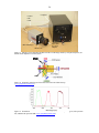
reflected from the first dichroic surface is directed via a prism reflection to the greenchannel CCD. Spectral trim filters are used to narrow each of these bands as follows:
green (500-580 nm), red (630-710 nm), and NIR (735-865 nm), approximating Landsat
bands. The optical layout is shown in Figure 14 and the spectral response curves for the
three channels are shown in Figure 15.
24
Computer
Camera
Link
Cable
MS3100 Imager
Nikon Lens
Super Fish
Eye Lens
Adapter
Figure 13: Imaging system including the MS-3100 three-CCD Imager made by Geospatial Systems, Inc.
and the small computer to run the system.
Dichroic
Surfaces
Prism
Figure 14: Schematic optical layout of the MS-3100 with color-infrared setup.
(www.geospatialsystems.com).
Figure 15: Transmittance of MS3100 channels in Color-IR mode. Green represents green, red represents
red, and dark red represents NIR (www.geospatialsystems.com).
25
The path length from the lens to each of the CCDs is the same and is equivalent to
the back focal length of the lens system. Each of the CCDs is 7.6 mm × 6.2 mm, with a
pixel size of 4.65 μm × 4.65 μm, which gives 1392 × 1040 pixels. The red and NIR
CCDs are monochrome CCDs, while the green CCD is tri-color and uses a demultiplexed
Bayer Pattern to achieve the green signal. The tri-color CCD captures RGB images and
outputs either RGB, demultiplexed red, demultiplexed green, or demultiplexed blue
images, depending on an input provided by the user.
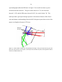
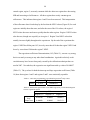
Even though I did not design and build the MS-3100 imager, I have modeled it
using the non-sequential mode in the Zemax optical design code (Figure 16). The prism
was not modeled and the dichroic surfaces were modeled as ideal (i.e., they reflect 0%
and transmit 100% or reflect 100% and transmit 0% of light). Zemax models dichroic
surfaces by placing them on a perfectly transmitting glass plate. The transmission and
reflectance characteristics of each dichroic surface must then be set for wavelength and
angle. For example, it is possible to set specific transmission and reflectance percentages
for specific wavelengths at specific angles of incidence. The CCDs are modeled with
appropriate spectral trim filters (Figure 15) intrinsic to the CCDs. The path lengths from
the back of the lens assembly to each CCD are set to 20 mm.
This optical model has been tested in Zemax using 15,000 analysis rays carrying a
total of 3 watts for the wavelength ranges of interest. The rays are randomly distributed
across the desired range of wavelengths. Two beams, 1.5 watts each, were modeled, one
centered on the optical axis and the other at the edge of the field. Figure 16 shows that
the colors are separated and sent to the correct CCDs, with the green rays representing
light within the green band, red rays representing light within the red band, and blue rays
26
representing light within the NIR band. In Figure 17, the results are shown as power
incident on the three detectors. The green sensor detected 1.17 W, the red sensor
detected 1.19 W, and the NIR sensor detected 0.64 W, for a total of about 3 W. This
model provided a good optical design experience with advanced features of the Zemax
code and enhances understanding of how the MS-3100 optical system directs color of the
proper wavelength to the proper CCD array.
Dichroic
Surfaces
CCDs
Figure 16: Zemax model of a MS-3100 3-chip multispectral imager. Here green represents the green color
plane, blue represents the red color plane, and red represents the NIR color plane, showing that the dichroic
surfaces are modeled effectively.
27
Figure 17: Power incident on modeled 3-chip imager detectors. These pictures show the central beam and
the edge-of-field beam, indicating that the optical system simultaneously produces proper images on each
of the three CCDs. The top is the green color plane, the bottom left is the red color plane, and the bottom
right is the NIR color plane.
One of the key requirements of this system was to image an area of approximately
10 m length (or larger) from the top of a scaffold whose height was best kept at or less
than approximately 6 m. Because of the very small size of the CCDs used in the MS3100 imager, it is quite difficult to achieve anything other than a very narrow field of
view (FOV). Initially I was using the short-focal-length, 14-mm, Sigma® lens sold with
the MS-3100 imager, which is usually a wide angle lens, but with the small CCDs our
full-angle horizontal FOV was only 24o. It turns out to achieve a shorter focal length
with a lens that mates properly to the MS-3100 imager required that I use a combination
of an old 20-mm, f/3.5, Nikon® lens and a 0.25x Phoenix® Super Fish Eye lens adapter
(see Figure 13) to decrease the focal length to effectively 5-mm and increase the fullangle horizontal FOV to 55o. The 20-mm lens was chosen since it has a relatively short
focal length and unlike newer lenses it does not have a tab near the threads that will not
28
allow them to connect to the MS-3100. The 20-mm lens was set to f/8 and focused at
infinity.
The MS-3100 imager interfaces to a control computer with a Camera Link
connection (Figures 18 and 13) that allows high-speed image data transfer to a National
Instruments PCI-1428 digital frame grabber card (Figure 19). This frame grabber allows
data to be transferred in base (8-bit) or medium (12-bit) Camera Link configuration.
Although the MS-3100 can record 8-bit or 10-bit images, we were not able to use the 10bit mode because the frame grabber needed either 8-bit or 12-bit data. Consequently, the
imager was run in 8-bit mode, giving us 0-255 digital numbers (DN) or grey levels for
each color plane.
Figure 18: Camera Link High Speed Digital Data Transmission Cable
(http://www.siliconimaging.com/ARTICLES/CLink%20Cable.htm).
29
Figure 19: NI PCI-1428 base- and medium-configuration Camera Link frame grabber card used to acquire
digital images from the MS-3100 imager (www.ni.com).
For the 2007 experiment, we used a Delta1 photographic grey card to calibrate the
imaging system in the field. Grey cards are designed to be lambertian reflectors, meaning
they reflect equal radiance at all angles. The grey card we used was designed to reflect
18% of the incident light, which is a common reflectance reference used by
photographers. For the 2008 experiment, we used a Labsphere Spectralon standard
(Figure 20) calibrated to 99% reflectance.
Spectralon
Figure 20: Spectralon reflectance standard mounted on tripod for continuous calibration of the MS-3100
imager during the 2008 ZERT field experiment (J. Shaw 2008).
In the 2008 experiment we chose to use spectralon instead of the grey card as a
calibration target because the grey card was found to have significantly non-Lambertian
30
reflectance, without an acceptably flat reflectance over 500-865 nm (Figure 21). The
spectralon was calibrated to reflect 99% of the incident light for illumination angles down
to 8o from normal, below which specular reflection becomes significant. Care must be
taken when using spectralon, in that it is very lambertian but its surface normal must be
oriented the same as the scene in question, or a cosine correction for the difference
between the illumination and viewing angles must be applied.
Figure 21: Reflectance spectrum of photographic grey card used to calibrate the MS-3100 imager during
the 2007 ZERT field experiment.
For the 2007 experiment we used a NI-USB 6210 digital/analog I/O module,
along with a National Semiconductor LM335 temperature sensor to measure the ambient
temperature around the imaging system. This was done in case a temperature response
correction was needed, but we found later that it was not needed because measurements
showed that the MS-3100 imager is very stable across the temperature range we
experienced in the field. To test this, in between the 2007 and 2008 experiments we
31
placed the camera in a thermal chamber and recorded dark-current images across a range
of temperatures greater than what we would see in the field without observing any
measurable change. This is described in more detail in Chapter 3
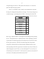
Spectrometer Hardware
Another optical sensor that was used extensively in this project was an Ocean
Optics USB4000 spectrometer (Figure 22). This is a fiber-fed hand-held spectrometer
that was used to measure the reflectance of calibration panels and vegetation. The optical
layout of this spectrometer is shown in Figure 23, with explanatory labels listed in Table
1. The spectrometer uses a Toshiba TCD1304AP Linear CCD array detector and
disperses light with a diffraction grating over a bandwidth of 350-1100 nm. There are
3648 pixels, each with a size of 8 μm × 200 μm. The spectral resolution of a pixel at fullwidth at half-maximum (FWHM) is approximately 0.21 nm. The aperture stop is 25 μm.
The analog-to-digital converter (A/D) resolution is 16 bits. A fiber optic cable provides
an easily hand-held input for the device. Data from the spectrometer are collected via a
USB cable with a laptop computer. For the measurements in this project, the data were
averaged over the MS-3100 bands for comparison with the multispectral imager data.
32
Serial
Interface
Cable
Computer
USB4000
Spectrometer
Fiberoptic
Cable
Small Spectralon
Sample
Figure 22: USB4000 Miniature Fiber Optic Spectrometer and Spectralon disk that were used together to
measure reflectance spectra of vegetation and calibration panels (www.oceanoptics.com).
Figure 23: USB4000 Miniature Fiber Optic Spectrometer Optical Layout (USB4000 Installation and
Operation Manual, www.oceanoptics.com).
33
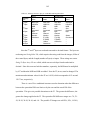
Table 1: USB4000 miniature fiber optic spectrometer optical layout
explanation (USB4000 Installation and Operation Manual,
www.oceanoptics.com).
Item Number
Name
1
SMA 905 Connector
2
Slit
3
Filter
4
Collimating Mirror
5
Grating
6
Focusing Mirror
7
L4 Detector Collection Lens
8
Detector
9
OFLV Filters
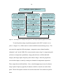
Imaging Software
I used multiple programs to fully implement the system and the calculations
needed to find reflectances. Various aspects of the task were implemented with NIIMAQ, DT Control, NI Measurement and Automation Explorer (MAX), NI LabVIEW,
NI Vision Acquisition, NI Vision Development Module, NI-DAQ, Ocean Optics
SpectraSuite, PcModwin 4.0 (MODTRAN), MATLAB, and solar position calculator,
Table 2 shows what routines are used by what programs, the purpose of each, and a
description of whether each was written as part of this project or obtained otherwise.
First the NI-IMAQ framegrabber software was installed, followed by the PCI1428 framegrabber hardware (Figure 19). This, along with a Camera Link cable (Figures
13 and 18), was used to interface the camera data output to the computer. I then installed
DT Control software (Figure 24), which is used to control the imager and optionally can
be used to acquire images. This program makes it possible to control the gain and
34
integration time (IT) separately for each color plane, overall exposure time, bit depth,
display modes, video mode (not used), triggers (not used), white balance (not used),
autoexposure controls (turned off), and image acquisition controls (not used). The
program also shows the status of the camera connections, such as the port used (control),
status of connection from last communication, image acquisition frame grabber (not
used), and status indicating if the imager is acquiring images.
Table 2: Listing of software programs used, routines used within each program, purpose for the program
and routine, and source of the software.
Software
NI
Measurement
& Automation
Explorer
(MAX)
NI-IMAQ (NI
Vision Acq. &
NI Vision
Dev.Module)
NI-DAQ
Routine
Interface imager and
temperature sensor
with computer
National
Instruments
Many
Image acquistion &
processing functions
National
Instruments
Temperature acquistion
& processing functions
2007 image acquisition
control program
2007 image postprocessing program
National
Instruments
Written
2008 image acquisition
and processing control
Written
Many
2. calculate reflection
(scaffolding_grey_multiple_scenes)2.vi
3. multiple extract planes & calculate
%reflectance without temp
sensor(2_with correction)_test2.vi
4. calculate reflection
(scaffolding_grey_multiple_scenes)3
SpectraSuite
N/A
MODTRAN
(PCModwin)
N/A
MATLAB
1. falloff_correction
2. create_refl_plot
3. create_refl_plot_min
R
Source
N/A
1. multiple extract planes.vi
NI LabVIEW
Purpose
Linear Model
2008 image postprocessing program
Spectrometer data
acquistion and
processing program
Irradiance modeling
program
Computes spatial nonuniformity correction
Plots reflectance, NDVI
Plots reflectance, NDVI
at min. point each day
Statistical Computation
Written
Written
Ocean
Optics
Ontar Corp.
Written
Written
Written
Rick
Lawrence
35
Figure 24: DT Control Main Camera control panel (DTControl Software Users Manual).
The gain control is used to amplify the output signal for each channel of the MS3100 separately, with a possible range of 2.0 dB to 36 dB. The integration time (IT) is
the amount of time the electronic shutter is ‘open’ and can be set for each channel. The
IT has a range of 0.12 ms to 130.75 ms. The overall exposure is used to change the
brightness of an image without changing the relative brightness of each of the color
planes. When this is changed, the individual ITs will be changed relative to each other.
The overall exposure is unitless and the min and max values are determined by each of
the channels ITs and the difference between these times.
The bit depth can be set to either 10 bit or 8 bit. However, the frame grabber we
used only allows for 8-bit or 12-bit data, so we used 8 bits. The display modes available
for the MS-3100 are CIR, RGB, Mono Red, Mono Green, Mono Blue, and Other. We
used CIR (color-infrared) which has NIR, Red, and Green channels. RGB is the typical
36
‘visible’ setup, which has Red, Green, and Blue channels. The three different Mono
setups output the selected color plane to all three channels. The Other selection is
specific to this MS-3100 setup and allows one of eight different outputs for each of the
channels: Red, NIR, Green/Blue, Processed Red, Processed Green, Processed Blue,
Processed Mono, and channel off. The ‘Processed’ options are the Bayer de-multiplexed
data from the tri-color CCD in the camera.
Next, the camera definition file was copied from the DTControl CD to the NIIMAQ Data folder. Then using MAX, the camera definition was activated so that a link
between the camera and NI software could be set up. To do this, Devices and Interfaces,
in the MAX Configuration Tree, was selected. This will show all of the NI devices
installed on the computer. Then by clicking NI-IMAQ Devices, all the NI-IMAQ devices
will be shown. With only one device connected, this shows ‘img0: NI PCI-1428,’ the
interface assigned for the specific frame grabber being used. Then by clicking on this,
the channel assigned for the imager, ‘Channel 0,’ is shown. Finally, the camera
definition file must be selected. To do this, right click the ‘Channel 0,’ select open
camera definition file, and then select the file copied earlier. At this point the camera is
ready to be used with LabVIEW, but LabVIEW must be readied.
Once LabVIEW is installed, NI Vision Acquisition and NI Vision Development
Module must be installed for full image acquisition and processing capability. NI Vision
Acquisition software is an application that will add a few virtual instruments (VIs, the
name of programs written in the LabVIEW graphical language) used to acquire, display,
and save images. NI Vision Development Module adds hundreds of VIs that allow highand low-level acquisition, display, processing, file I/O, pattern matching, particle
37
analysis, measurement tools, amongst many others. We used only a few of the VIs that
came with the NI Vision Development Module. Now the imager can be easily interfaced
with LabVIEW. LabVIEW was used for image and temperature acquisition in 2007 and
image acquisition and processing in 2008.
2007 Experiment:
For the 2007 experiment the programs multiple extract planes.vi and calculate
reflection (scaffolding_grey_multiple_scenes)2.vi were used. The first program acquires
images of the vegetation test strip, saves the temperature during an image acquisition, and
saves pixel value arrays of each of the color planes and the calculated NDVI. The second
program was used to calculate reflection and NDVI using only images of the vegetation
with the photographic grey card calibration target in the image. This program uses
regions of interest (ROIs) to select the grey card and three separately analyzed vegetation
regions within both the mown and un-mown segments of the test area. The second
program provided only a few calibrated images each day, but was used after two other
attempted calibration methods did not work sufficiently well. These initial calibration
methods were based on 1) using gray card images recorded whenever the IT changed,
and 2) using continuous measurements of solar irradiance at the surface. The lack of
success of these methods was because the periodic grey card images did not track
conditions as they changed with sun angle or clouds and because the location of the solar
irradiance measurements was too far distant from the ZERT test site. These two
calibration methods will be described in more detail in Chapter 4, Section 2.
38
multiple extract planes.vi
Create a folder to place image
pixel value arrays and a
spreadsheet for temperatures.
Initialize image capture
session and configure image
buffer list.
User supplies temperature
sensor channels, camera
interface name, image
capture frequency, and paths
to image and temperature
files. Then user starts the
program.
Configure buffer image type
and initialize asynchronous
image acquisition.
Enter timed loop with the
image capture frequency set
by the user to control how
often to image.
Set up image references for
the three color planes and
arithmetic functions needed to
find NDVI.
Grab image data from buffer
and display images on front
panel.
Finds present time for file
name identification, converts
and saves each color plane as
an array of pixel values
Acquire temperatures, convert
to Celsius, and save to the
temperature spreadsheet.
Close current image and
temperature acquisition
Loop back to acquire another
image after the allotted image
capture frequency.
Figure 25: Flow diagram for ‘multiple extract planes.vi,’ the image acquisition program used in 2007.
To run the primary image acquisition program used in 2007, multiple extract
planes.vi (Figure 25), a folder must be created to hold the measured image arrays. The
user must also supply the following inputs: temperature sensor channel numbers
(channels 1 and 2 on the USB-6210), camera interface name (‘img 0’), temperature path
(reference to temperature spreadsheet), image path (reference to folder that holds
images), and image capture frequency (how often to image). Once the program has
received these inputs, it starts by creating two channels for temperature acquisition.
These output data are held until later. Next, a timed imaging loop was used so that an
image capture frequency (typically 10 minutes) could be set by the user on the front
panel. Then a flat sequence structure was used to insure that VIs would run at specific
times.
39
The LabVIEW program is a graphical routine divided into a sequence of panels,
as indicated in Figure A2 of the Appendix. Panel 1 of the flat sequence initializes an
image capture session and configures a buffer list to place the images for processing.
Panel 2 configures the buffer for the specific image type and starts an asynchronous
acquisition. The buffer image type is ‘Grayscale (U8).’ Panel 3 sets up image references
for each of the three color planes and for two arithmetic functions used to find NDVI. I
gave these the image names ‘Green,’ ‘Red,’ ‘NIR,’ ‘minus,’ and ‘plus.’ These are passed
to the buffer for identification later. Panel 4 grabs data from the buffer, displays the
images on the front panel and calculates values needed to calculate NDVI. Initially the
CIR image is displayed, then the CIR image is split into its component color planes and
they are displayed on the front panel. The red color plane is subtracted from the NIR,
pixel-by-pixel, to find the numerator for the NDVI calculation (Eq. 1) and the difference
is normalized by the sum of these two images to obtain the NDVI. Panel 5 finds the
present time and converts and saves image color planes and NDVI data into arrays of
pixel values. The arrays are saved with a file name consisting of the color plane name
concatenated with a time stamp so that each image’s time is saved.
Panel 6 acquires two temperatures, one near the imager and one at the back of the
computer, converts them to degrees Celsius, and saves them to a temperature array. The
samples were converted to Celsius using the following equation.
Tcelsius =
Tsample − 2.982
0.001
+ 25
In this equation Tsample is a 2-D representation of the voltages (proportional to
temperature) sampled by the NI-USB 6210 and Tcelsius is a 2-D representation of the
temperatures in Celsius. The temperatures are read into a 2-D Waveform Chart.vi to
(2)
40
display both temperatures on the screen in real time. At this point the flat sequence
structure has finished, so the present image acquisition is closed. Now the system will
loop back to Panel 1 of the flat sequence structure after the time corresponding to the
image capture frequency has passed. When the system is shut down for the day, after all
the images have been acquired, the program will exit the imaging loop. At this point
calculate reflection (scaffolding_grey_multiple_scenes)2.vi must be run to calculate
reflectance and NDVI. The NDVI is calculated again since the calculation done during
the image acquisition program was not done correctly, in that NDVI was calculated from
unbalanced average DNs instead of radiometrically calibrated reflectances.
The program calculate reflection (scaffolding_grey_multiple_scenes)2.vi
calculates reflectance and NDVI for three regions using ROIs for one specific day, Figure
26. There is an ROI for each color plane in each vegetation region studied, and for each
color plane for the calibration target, which gives 12 ROIs. The program will display
each of the scene’s average DN and the reflectance for each region. To start this
program, the user must supply the path to the image folder and a path to a
%reflectance/NDVI spreadsheet. This spreadsheet must already be created with 15
columns and enough rows to hold data for every image taken during one day. Once these
paths are entered, the program can be started.
41
calculate reflection (scaffolding_grey_multiple_scenes)2.vi
Create a %refletance/NDVI
spreadsheet.
Enter for loop, where each
iteration is a
%reflectance/NDVI
calculation for one image.
User supplies path to folder of
images and
%relfectance/NDVI
spreadsheet. The program can
be started
Read file name out of the file
name array at the associated
iteration and save this to
%reflectance/NDVI
spreadsheet as a reference for
the calculated %reflectance
and NDVI
Reads file names from image
folder and stores in 1-D array.
Counts files for number of
loop iterations needed.
Query file name for color
plane, so that the correct
algorithm can be applied.
Calculate average DN for
each vegetation region and the
calibration target using
regions of interest.
Calculate and save reflectance.
Complete all loop iterations,
computing all reflectances.
Open %reflectance/NDVI
spreadsheet, calculate and
save NDVI.
Figure 26: Flow diagram for ‘calculate reflection (scaffolding_grey_multiple_scenes)2.vi’, the
%reflectance and NDVI calculation program used in 2007.
The program (Figure A4 of the Appendix) starts by reading the file names at the
given folder path and storing them in a 1-D array so that they can be called one at a time
for calculations. An example file name is 125432 PMNIR, where the first six digits are
the time of the image and the first two letters after the space indicate morning or
afternoon (12:54:32 PM). The rest of the file name is the color plane the image refers to:
IR is Near-infrared, R is red, and G is green. For images that have the grey card present,
‘grey’ would be added to the end; for example, if the file name mentioned above were a
grey card image, it would be 125432 PMNIRgrey. Next a For loop is entered, where
each iteration calculates reflectance and NDVI for the ROIs for a specific file.
Within the loop the first file name is read and is appended to the folder path, so
that it can be opened in the future. The file name is then displayed on the front panel so
the user knows what the current file is. This file name is then saved to the
42
%reflectance/NDVI spreadsheet set up by the user. Now a query is performed on the file
name to determine which color plane it is, so that the correct algorithm can be applied.
Once the program has figured out what color plane the file is, the file is opened and the
pixel values are then sent to ROI average calculators, which calculate the average DN of
the selected ROI. The array is displayed on the front panel using an intensity graph with
scroll bars to determine the ROI. The user is able to move the scroll bars to define the
ROI. The ROI average calculator will loop until the user presses the stop button, insuring
the best possible region has been chosen. Next, the reflectance is calculated using
Equation 3, with values specific to each color plane’s spectral band dark current and grey
card reflectance. These values are seen in Table 3.
⎛
DN
− DN
⎞
λ , scene
λ , dark
⎟ * ρ λ ,calibration target
ρ λ = ⎜⎜
⎟
−
DN
DN
λ
,
calibratio
n
t
arg
et
λ
,
dark
⎝
⎠
(3)
Finally, the reflectance is saved to the %reflectance spreadsheet. The row index is
controlled by the iteration index and the column is controlled by the color plane of the
image and the ROI index (1, 2, or 3). The first column holds the time. The second, third,
and fourth columns will hold the Green, Red, NIR reflectances, respectively, for the first
region. The sixth, seventh, and eighth columns hold the Green, Red, NIR reflectances,
respectively, for the second region. The tenth, eleventh, and twelfth columns hold the
Green, Red, NIR reflectances, respectively, for the third region. Once all of the
reflectance calculations have completed, the arrays are opened once again and NDVI is
calculated by accessing the appropriate cells. The array is saved one final time and
program finishes. At this point, MATLAB was used to plot the reflectances for each
region, 1, 2, and 3, in the mown and un-mown areas.
43
Table 3: Values Used to calculate reflectance for each of the color planes during the 2007
experiment with the photographic grey card.
Value
Color Plane
Green
Red
NIR
Dark Current (DN)
Spectral Reflectance of
Grey Card
1.34
1.43
1.79
22.83%
18.172%
17.373%
2008 Experiment:
For the 2008 experiment, a spectrally flat 99% reflective spectralon panel was
mounted permanently within the imager’s FOV to provide continuous calibration. The
imager was controlled with the program multiple extract planes & calculate %reflectance
without temp sensor(2_with correction)_test2.vi (Figure 27). The block diagram for this
program can be seen in Figure A6 of the Appendix. This program runs autonomously
once started. It changes the IT of the imager to maintain the brightness of the spectralon
calibration panel within a specific range set by the user, thereby keeping the balance of
incident light between the three CCDs constant. This makes it possible to get good
measurements in sunny or cloudy conditions since the spectralon is viewed in every
image. The vegetation and calibration regions are chosen with user-defined ROIs. The
program will then calculate % reflectance and NDVI for three regions and display the
results in real time on a graph. Finally, the program saves the results to a spreadsheet.
44
multiple extract planes & calculate %reflectance without temp
sensor(2_with correction)_test2.vi
Create a folder to place image
pixel value arrays and a
spreadsheet for %reflectances.
User supplies camera
interface name, image capture
frequency, paths to image and
%reflectance files and limits
for spectralon DN as a IT
control. Then user starts the
program
MATLAB script node opens
CCD spatial non-uniformity
correction arrays
Enter timed loop with the
image capture frequency set
by the user to control how
often to image.
MATLAB corrects image data
for spatial non-uniformity.
Finds present time for file
name identification, converts
and saves each color plane as
an array of pixel values
Grab image data from buffer
Configure buffer image type
and initialize asynchronous
image acquisition.
Set up image references for the
three color planes
Set up and display each
region’s reflectance and
NDVIs on four different realtime graphs.
Set up image references for the
three color planes
Configure buffer image type
and initialize asynchronous
image acquisition.
Initialize image capture
session and configure image
buffer list.
Enter IT control loop.
Initialize image capture
session and configure image
buffer list.
Calculate average DN for
vegetation scenes and
spectralon using ROI.
Close current image
acquisition
Calculate average DN for
spectralon using ROI.
MATLAB corrects image data
for spatial non-uniformity.
Grab image data from buffer
Close current image
acquisition.
Loop back to acquire another
image after the allotted image
capture frequency
If all three are color plane ITs
are correctly set continue with
image acquisition.
Check if current IT gives
average DN for spectralon that
falls within the range set by
user, for each color plane.
If one or more ITs are not
correct continue with IT
control loop.
Figure 27: Flow diagram for multiple extract planes & calculate %reflectance without temp sensor(2_with
correction)_test2.vi, the image acquisition, reflectance and NDVI calculation program used in 2008.
To run the program, a folder must be created to save the images and a
%reflectance spreadsheet. The %reflectance spreadsheet must also be created with a
45
layout of 19 cells wide and about 75 cells long. The length depends on how long imaging
will take place and the image capture frequency. The cells should be filled initially with
zeros. The first column is used to hold the time of each %reflectance measurement. The
second, third, fourth, and fifth columns hold the Green, Red, NIR reflectances, and
NDVI, respectively, for the first region. The seventh, eighth, ninth, and tenth columns
hold the Green, Red, NIR reflectances, and NDVI, respectively, for the second region.
The twelfth, thirteenth, fourteenth, and fifteenth columns hold the Green, Red, NIR
reflectances, and NDVI, respectively, for the third region. The seventeenth, eighteenth,
and nineteenth columns hold the ITs for the Green, Red, and NIR color planes,
respectively, for that specific image. The user must also supply some inputs: camera
interface name (‘img 0’), image path (directory to save images to), %reflectance path,
image capture frequency (how often the imager should image), and the upper and lower
limits for the average DN of the spectralon desired for each color plane (determines how
sensitive the IT control will be).
The program starts by calling a MATLAB script node to open spatial nonuniformity corrections arrays, discussed in detail in Chapter 3, for each color plane and
save these to arrays for later use. These are linear correction functions that are
implemented as offset and gain arrays for each pixel of each color plane. MATLAB was
implemented multiple times in this program to speed up its process time.
A timed loop
was then called so that an image capture frequency (typically 3 minutes) could be set by
the user on the front panel. Each iteration of the loop corresponds to one image for each
color plane. Then a flat sequence structure was used to insure that VIs would run at
specific times.
46
Panel 1 contains the entire IT control code. A conditional loop is used to
continually change the IT until all three color planes are within the user-specified range.
Within this loop there is a flat panel structure. Having a secondary flat panel within the
main flat panel could cause confusion in this discussion, so for clarity this discussion will
refer, for example to panel 1-2 when referencing the main panel 1 and secondary panel 2.
Panel 1-1 initializes an image capture session and configures a buffer list to place the
images for processing. Panel 1-2 configures the buffer for the specific image type and
starts an asynchronous acquisition. When the imager is running in 8-bit mode, the image
type is ‘Grayscale (U8).’ Panel 1-3 sets up image references for each of the three color
planes. I gave these the Image Names ‘Green’, ‘Red’, and ‘NIR’. Panel 1-4 grabs data
from the buffer, separates the three color planes, and converts the images to arrays of
pixel values. Panel 1-5 is for the spatial non-uniformity correction, implemented with a
MATLAB script node. The scene is corrected using Equation 4, shown for the NIR color
plane but available for implementation with any color plane.
NIR _ scene _ cor = ( NIR _ scene * NIR _ gain _ array ) + NIR _ offset _ array
(4)
Panel 1-6 sends corrected scene pixel values to the ROI average calculators,
which calculate the average DN of the selected ROI, in this case the exposure control
ROI. First of all the array is displayed on the front panel using an intensity graph with
scroll bars to determine the ROI. The user is able to move the scroll bars to define the
ROI. The average of the ROI array is found, panel 1-7 closes the current image
acquisition, panel 1-8 causes the program to wait for 5 seconds before moving on to the
next panel, and panel 1-9 contains a third flat sequence structure that checks the pixel
values within the calibration target area and adjusts the IT if they are no longer within the
47
average DN range set by the user. These panels will be denoted as 1-9-1 for the first
panel of the third flat sequence structure.
Panel 1-9-1 is the NIR IT control. Initially, serial communication is setup with
the imager for reading and writing attributes to the imager. The serial port settings are set
to match the imager’s serial settings shown in Table 4. Next, the panel reads the NIR
Table 4: Serial settings needed to communicate with the MS-3100 imager.
Input Setting
Value
Enable Termination Character
TRUE
Termination Character
A
Timeout (ms)
5000
Baud Rate
9600
Data Bits
8
Parity
NONE
Stop Bits
1
Flow Control
NONE
ROI average, computed in Panel 1-6, and compares it to the NIR upper limit provided by
the user. The program then uses a conditional structure, which, depending on if the DN
is greater than or less than the upper limit, will start the process to lower the IT or check
the lower limit, respectively. If the DN is less than the upper limit, the spectralon
average DN is compared to the lower limit and another conditional structure is used,
which, depending on if the DN is greater than or less than the lower limit, will either exit
without changing the current IT with a true state (indicating the IT is set correctly), or it
will start the process to increase the IT. Since the processes to increase or decrease the IT
are the same, I will explain just the method to increase the IT.
48
Initially the imager is queried and current attributes are read. When the imager is
queried and the imager buffer is read, 6 Bytes are written and 9 bytes are read. If the
imager is sent a command to change its attributes, 8 Bytes are written and 6 Bytes are
read. The messages are in hexadecimal and if querying or setting the IT, the messages
have the following format.
Table 5: Message format to query or set the MS3100 integration time.
Query
Set Attributes
Message
Write
Read
Write
Read
Byte
0th Byte
1st Byte
2nd Byte
3rd Byte
4th Byte
5th Byte
6th Byte
7th Byte
8th Byte
Start Byte
LSB Size
MSB
Size
Command
Byte
Channel
Number
Checksum
----
Start Byte
LSB Size
MSB
Size
Command
Byte
Channel
Number
IT (LSB)
IT (MSB)
Status
Checksum
Start Byte
LSB Size
MSB
Size
Command
Byte
Channel
Number
IT (LSB)
IT (MSB)
Checksum
--
Start Byte
LSB Size
MSB
Size
Command
Byte
Status
Checksum
----
The check sum is the 8-bit, two’s complement of the message bytes. The message bytes
in a query are the command byte and channel number, and the message bytes in a set
attribute command are the command byte, channel number, IT (LSB), and IT (MSB).
For a more detailed description of serial communication with the MS3100, consult the
‘MS2100, MS2150 & MS3100 Digital Multispectral Camera User Manual.’ Next, the 5th
and 6th bytes are read and converted to decimal format. The IT is then changed according
to an algorithm that checks how far from the acceptable range the current IT is. This
algorithm also checks that the new IT is within minimum, 0, and maximum, 1024, values
for the IT, which correspond to 0.12 ms and 130.75 ms, respectively. There is a set of
five conditional structures used to determine the difference between the spectralon DN
49
lower limit set by the user and the actual DN. This gives six possible alterations to the
IT. The greater the difference, the greater the change applied to the IT. The spectralon
DN difference ranges are >70, 70-50, 50-30, 30-20, 20-10, and <10. The possible IT
changes are add 50%, 20%, 14.28%, 11.11%, 8.33%, and 6.67%, respectively. For the
decrease in IT, the IT changes would be subtracted from the original IT instead of added.
The message to set the IT is sent, but first the new IT is converted to a hexadecimal
number and the checksum byte of the message to change the IT is calculated. A false
state is returned after the IT has been changed so that the program knows it will need to
check the spectralon DN at least one more time before imaging. Once the NIR IT check
has finished, the red (Panel 1-9-3) and then the green (Panel 1-9-5) color planes are
checked. After all color planes have been checked, both interior flat sequence structures
are exited and the logical statements indicating whether or not each color plane’s IT are
correctly set are checked to see if all three are correct. If not, the program loops back to
panel 1-1; if so, the program moves ahead to panel 2 to begin the vegetation imaging.
Panel 2 of the main flat sequence initializes an image capture session and
configures a buffer list to place the images for processing. Panel 3 configures the buffer
for the specific image type and starts an asynchronous acquisition. Panel 4 sets up image
references for each of the three color planes. These have the image names ‘Green,’
‘Red,’ and ‘NIR.’ Panel 5 grabs data from the buffer and separates the three color planes
into separate images. Panel 6 finds the present time and converts and saves image color
plane data into arrays of pixel values. The arrays are saved with a file name consisting of
the color plane name concatenated with a time stamp so that each image’s time will be
saved. Each of the images was saved so that post-processing may be done. Panel 7 is for
50
spatial non-uniformity correction. A MATLAB script node was used here. The scene is
corrected using Equation 4, which uses the NIR color plane as an example. Panel 8 sends
corrected scene pixel values to the ROI average calculators, in this case the spectralon
and vegetation ROIs (there are three vegetation ROIs for each color plane). The
corrected arrays are displayed on the front panel using an intensity graph with scroll bars
to determine the ROI. The user is able to move the scroll bars to define the ROI.
Reflectance is calculated using Equation 3 using the dark current values listed in Table 3,
the spectral reflectance of 99%, the spectralon average DN, and scene average DN.
NDVI is found using Equation 1, and the reflectances, NDVI, and ITs are saved to the
%reflectance spreadsheet using the format discussed earlier.
Panel 9 sets up the initial X and Y axes for the real-time displays for reflectances
and NDVIs. The real-time graphs are initialized on the first iteration of the imaging
cycle. Panel 10 updates the X-axis and data points of the real-time graphs, displaying all
reflectances and NDVI data points on one of four graphs. Each region’s reflectances are
shown on separate graphs and the NDVI values for each region are shown on a graph.
Panel 11 finishes the current image acquisition process. At this point, the system will
loop back to Panel 1 of the flat sequence structure after the time corresponding to the
image capture frequency has passed. When the system is shut down for the day after all
the images have been acquired, the program will exit the imaging loop and close the
program.
For image post processing I wrote a program, calculate reflection
(scaffolding_grey_multiple_scenes)3, which loads the vegetation images and calculates
reflectances and NDVI using ROIs. This program is the same as calculate reflection
51
(scaffolding_grey_multiple_scenes)2, except a more efficient code to read images and to
write the %reflectance/NDVI spreadsheet was adopted.
The 2007 or 2008 reflectance and NDVI files can be viewed graphically using the
MATLAB codes create_refl_plot_’segment’ or create_refl_plot _’segment’_min. The
first program plots every reflectance and NDVI measurement for every day, while the
second program plots only the minimum reflectance and NDVI at times corresponding to
the maximum solar angle for each day. The value ‘segment’ must be either mown, unmown, or plants8910. The only difference between these is that the titles used on the
plots are changed to distinguish between each segment. These programs will also plot a
first-order fit to the minimum points, to help the viewer get a better idea of the total
trends. In addition, 95% confidence intervals were plotted. Finally, R2 and p-value
values are output from these programs for analysis of data, more specifically goodness of
fit and statistical significance, respectively.
52
IMAGING SYSTEM CHARACTERIZATION AND CALIBRATION
To ensure good calibration of images acquired in the field, I tested the imaging
system for potential causes of error. Much of this characterization work came about as
part of an investigation of calibration accuracy using two spectralon panels. I wanted to
test the system by using one spectralon panel to calibrate images while using the other as
a test target, since both are of known reflectance. Spectralon is nearly perfect for this
since it is a nearly lambertian surface. The two spectralon targets used here are rated at
50% and 99% reflectance. Equation 3 was used to calculate reflectance.
On a clear day, I set up the imager so that it viewed both panels simultaneously.
Imager attributes were set to similar values used in the ZERT field. Then using the
LabVIEW VI multiple extract planes & calculate %reflectance without temp sensor.vi,
which is the same as multiple extract planes & calculate %reflectance with temp
sensor.vi except without temperature measurements, I placed the ROIs on each of the
spectralon panels. The calibration target ROI was placed on the 99% panel and the scene
ROI was placed on the 50% panel. We would therefore expect to get ~50% reflectance in
the output file for each color plane, but we obtained values near 60%. Then we changed
the test by making the 99% panel the scene and the 50% panel the calibration panel and
we obtained values of about 80%. So both tests were off by about 20% of what they
should be.
These calibration panel tests were repeated with the imager attributes set to values
that reduced the amount of light that reached the CCDs to a minimum. This was done by
decreasing the gain and integration time and increasing the F/#. This made it possible to
obtain correct reflectance values, but it reduced the dynamic range of the system so much
53
that it would not be effective in the field (the 99% panel only registered a DN of 15,
whereas the full possible range of the system is 255 DN).
We were told by the manufacturers of the MS-3100 that the imager was very
linear no matter what attribute was changed, but we wanted to make sure. From an
educational engineering stand point this is important to me so that I have a better
understanding of the response of the imager. Therefore, I tested DN vs. integration time,
DN vs. gain, DN vs. F/#, DN vs. radiance, DN vs. temperature, DN vs. polarization
angle, a pixel’s ability to quickly drain charge when viewing a dim scene after viewing a
very bright one, pixel smear, and spatial non-uniformity. I found that the imager works
very well under the conditions we exposed it to in the field. The only problem that
required compensation was a spatial non-uniformity, caused presumably by the extrawide-angle lens adapter used to increase the imager’s field of view. However, we
corrected for this by finding and applying a linear fall-off correction to each pixel.
Towards the end of the experiment, I also characterized the angular reflectance properties
of a spectralon panel to gain a better understanding of lambertian surfaces.
Initially, I believed these problems could be attributed to one or more of the
following: a change in integration time, gain, F/#, or radiance. To test these we operated
the imager looking into an integrating sphere to ensure spatially uniform radiance across
the CCDs. We then changed one of the attributes while keeping all others constant. The
average DN for the entire scene was then plotted versus the attribute change. We also
explored the spatial variation of DN for this uniform scene, which led to the nonuniformity correction described later.
54
The integration time is the amount of time, in milliseconds, that the electronic
shutter is ‘open’. This can be set for each CCD separately. The gain was set to 2 dB, 4
dB, and 4 dB for the green, red, and NIR planes, respectively. The F/# was set to 11 and
the focus was set to approximately 25 cm. I initially ran this test for integration times
over the range of 1-130 ms in increments of 5 ms. The resulting plot, Figure 28, shows
that the red and NIR CCDs are fairly linear in response to a change in integration time,
but that the green plane has the smallest linear range. I then noticed the response seemed
very linear for all the CCDs in the range from 1-20 ms, which is the working range used
in the field for our experiments. Figure 29 shows the response over this limited range of
ITs. The R2 values are 0.9812, 0.9995, and 0.9998 for the green red and NIR color
planes, respectively. Luckily, the green plane is not as important to us as the red and NIR
planes.
Figure 28: A plot of the average digital number for each color plane as a function of integration time. The
full range of integration times, 1-130ms, is shown here.
55
Figure 29: A plot of the average digital number for each color plane as a function of integration time. The
full working range of integration times, 1-20ms, is shown here.
Next, we tested the linearity of signal with a change in gain. The gain setting
changes the settings on the electronic amplifiers used to amplify the signals read from the
CCDs. These amplifiers can easily have significantly nonlinear behavior. The
integration time was set to 3 ms, 5 ms, and 5 ms for the green, red, and NIR planes,
respectively. F/# was set to 11 and the focus was set to 25 cm. The gain values are in
dB, so I converted them to a linear scale (gain (linear) =10(gain (db)/10)). Figure 30 shows
that the CCDs’ responses over the full gain range are very nonlinear. But, if only the
working range is considered, it looks much more linear, as shown in Figure 31. The R2
values are 0.9850, 0.9848, and 0.9847 for the green red and NIR color planes. Again,
when the system is in the field the gain is not changed, so this was determined not to be
the source of our observed calibration problem.
56
Figure 30: A plot of the average digital number for each color plane as a function of gain. The full range
of gains, 2-36 dB or 1.585-3981 on a linear scale, is shown here in a linear scale.
Figure 31: A plot of the average digital number for each color plane as a function of gain. A range of
gains, 2-12 dB or 1.585-15.85 on a linear scale, is shown here in a linear scale.
57
Next we plotted the average DN versus a change in F/#, as shown in Figure 32.
Changing the F/# by manually turning the aperture ring on the manual focus Nikon lens
changes the diameter of the entrance pupil, which in turn changes the amount of light that
reaches the CCDs by allowing light to be gathered over a larger portion of the lens. The
gain was set to 5 dB, 10 dB, and 10 dB for the green, red, and NIR planes, respectively.
The integration time was set to 3 ms, 5 ms, and 5 ms for the green, red, and NIR planes,
respectively. The focus was set to 25 cm. Here the average DN is plotted versus
1/(F/#)2, since this value is proportional to the power on the CCDs. The R2 values are
0.9995, 0.9995, and 0.9996 for the green red and NIR color planes, respectively.
Figure 32: A plot of average DN as a function of (F/#)-2.
58
Next the radiance from the integrating sphere was changed while the camera
settings were maintained constant. The radiance was changed by altering the current to
the light bulb in the sphere. The gain was set to 3 dB, 5 dB, 5 dB for the green, red, and
NIR planes, respectively. The integration time was set to 18 ms, 25 ms, and 33 ms for
the green, red, and NIR planes, respectively. The F/# was set to 11 and the focus was set
to 25 cm. In Figure 33 the horizontal axis shows the current measured by a detector in
the sphere and the vertical axis shows the average DN measured by the MS-3100. Again,
the green exhibits the most non-linear behavior, but the red and NIR planes are quite
linear. This means that in the field the camera settings should be adjusted so that the 99%
spectralon panel registers less than about 180 DN for the green color plane to avoid
saturation. Since the green channel is obviously non-linear past 180 DN and it was never
run in that regime the linear fit only considers points of 180 DN and less. The R2 values
are 0.9963, 0.9957, and 0.9976 for the green red and NIR color planes, respectively.
Figure 33: Average DN measured by the imaging system when viewing the integrating sphere, plotted
versus current measured by the integrating sphere’s detector.
59
Next I examined the response of the imager to temperature changes. To do this I
set the imager’s attributes to values similar to those used in the field (the gain was set to 3
dB, 5 dB, 5 dB and the integration time was set to 18 ms, 25 ms, and 33 ms for the green,
red, and NIR planes, respectively). The lens cap was left on so that we would measure
only the dark current. The imager was placed in a darkened thermal chamber and the
temperature was increased from 18oC to 43oC in 5oC increments. After each temperature
change the imager waited until it was at an equilibrium temperature before recording
images. All pixels of the imaging array were averaged, giving an average DN for each
color plane. I found that across the temperatures evaluated, there was only a change of
about 0.07 DN for the green color plane, 0.04 DN for the red color plane, and 0.02 for the
NIR color plane, as shown in Figure 34. I also found that the standard deviation of the
spatial variation of dark noise was very low: 1.79 DN for the green color plane, 1.34 DN
for the red color plane, and 1.43 DN for the NIR color plane.
Figure 34: A plot of the effect of camera temperature on the imager’s response.
60
I also tested the response of the imager to a changing polarization state for the
incoming light. Again, I set the imager’s attributes to values similar to those used in the
field: the gain was set to 3 dB, 5 dB, and 5 dB and the integration time was set to 18 ms,
25 ms, and 33 ms for the green, red, and NIR planes, respectively. I set up the imager to
view the integrating sphere through a rotating linear polarizer. It was found that the
imager’s signal changes less than 1% for different polarizer angles, as shown in Figure
35.
Figure 35: A plot of the affect of polarization angle on the imager’s response.
None of the characteristics investigated so far were determined to be the cause of
the abnormally high and low signals found when viewing the 50% and 99% Spectralon
panels. So, after some more brainstorming I came up with some more possibilities. First,
I thought maybe the CCDs were not able to drain charge quickly after viewing in bright
61
conditions, which could lead to a build up of residual charge in the pixels and could be
seen as an increase in the dark current. Also, there may be a ‘bleeding’ effect as the
charge is read out from the CCD, causing a streak of higher pixel values in the direction
of the walk off (this effect is frequently observed as bright streaks emanating from bright
portions of an otherwise dark image). Lastly, there may be a spatial non-uniformity,
which is usually present with CCD imagers and may be augmented by the super-wideangle lens adapter used to increase the small FOV of the imager.
To test the CCDs’ ability to drain charge, the system was again set up to view the
integrating sphere. The dark current was first measured by placing the lens cap on the
imager. Then images were acquired every thirty seconds for an hour, during which time
the imager was continually illuminated with bright light. A DN was read out at the
beginning and end of the bright conditions. At the end of an hour of bright illumination,
the dark current was measured again. As can be seen in Table 6, the CCDs drain charge
very effectively, since the dark current returns immediately to the initial values after
viewing bright light.
Table 6: Values obtained in a test of the CCDs ability to quickly drain charge after viewing bright
conditions.
Green (DN) Red (DN) NIR (DN)
Dark current before bright condition
0.02
0.5
0.7
DN at beginning of bright conditions
182
149
164
DN at end of bright conditions(1hr elapsed)
189.9
156.3
170.45
Dark current after bright condition
0.02
0.5
0.7
To see if there is a ‘bleeding’ effect, the imager was moved to a larger distance
from the integrating sphere so the sphere only filled a small center portion of the imager’s
62
FOV. Then the DN was measured around the bright spot created by the sphere, showing
that there is a very small ‘bleeding’ effect in the read-out direction (to the right when
viewing an image), but this effect is only about 1 part in 255, as indicated in Table 7.
Table 7: Bleeding effect caused by CCD charge 'walk-off' (DN on a scale of 0-255).
Green (DN)
Red (DN)
NIR (DN)
DN in read-out direction
0.64
1.1
1.4
DN not in read-out direction
0.1
0.1
0.25
Finally, I investigated the spatial non-uniformity of the CCDs. To do this I
viewed a spectralon panel with the FOV filled and I definitely saw a fall off of image
brightness toward the edges. When comparing the center pixels to the edge pixels, there
was almost a 50% fall off. To correct this, we decided to apply a unique linear signaldependent calibration function to each pixel of each CCD (where the variable is the DN
of the pixel). To find the gain and offset of these functions, I constructed a linear fit to
five images: one dark image with the lens cap on, an image of each spectralon panel
(50% and 99% reflective) filling the FOV in direct sunlight, and an image of each
spectralon panel filling the FOV in shaded conditions.
A MATLAB script was created that could quickly handle the large image files
used to process these calibration data. The script starts by opening an image file. Then it
finds an average value, the expected value for all pixels, for a 20×20 array of pixels right
in the center of the pixel array, for each image. It then places these values into a 1×5
array that contains the expected value for all pixels in each image. Then the uncorrected
image arrays are placed into a 1040×1391×5 array, where the first two dimensions are the
image array dimensions and the last dimension is the image number.
63
Next, two for loops are set up, one the size of the x-dimension and one the size of
the y-dimension of the image array, so that each pixel is tested and will have a linear
correction function. Inside the loops, the linear fit starts by placing the pixel values for
all images for the 1st index of both dimensions of the image array, pixel (1,1), into an
array. This is a 1×5 array of uncorrected pixel values. Then the MATLAB ‘polyfit’
function was used to make a 1st order fit of the uncorrected pixel values to the expected
values. The function returned the gain and offset (slope and intercept of the best-fit line),
which were placed in separate arrays at indices corresponding to the pixel indices. The
loop then continued until all pixels had a linear fit. Finally, the gain and offset arrays
were saved to a file to be accessed when future images are captured. The program was
run for all three color planes. The correction is applied during imaging by reading the
uncorrected pixel values into a MATLAB script that uses Equation 4 (shown with the
NIR color plane as an example) to correct the pixel values. Uncorrected (Figure 36) and
corrected (Figure 37) plots of the uniformly illuminated images for the Red color plane
are shown below.
64
Figure 36: 3-D view of uncorrected red color plane image viewing an evenly illuminated scene.
Figure 37: 3-D view of corrected red color plane image viewing an evenly illuminated scene.
65
Even after the spatial uniformity correction, the problem has not been corrected,
even though it has been improved. However, finally it was found that the spectralon
reflectance changes with the illumination angle (Labsphere, Inc. 2006). Consequently, as
the illumination angle increases there will be an increasing error in reflectance. Initially I
had kept the solar illumination angle somewhat high (near 60°) and tried to view the
panels near normal incidence to ensure that the imager did not view a specular reflection.
As seen in Table 8, this geometry was causing an error in measured reflectance,
especially in the 50% panel (assuming a 60% panel is similar to a 50% panel).
Table 8: Change in reflectance of spectralon due to illumination angle (measured from the surface normal)
for 99% and 60% panels (Labsphere, Inc., 2006).
According to this chart, we may be seeing a 5% change of the nominally 50%
reflectance due to illumination angle, which corresponds to a reflectance increase of
2.5%. That is, a nominally 50% reflectance panel will see a 5% change in its total
reflectance, which would make it appear as a 52.5% reflectance panel when viewed at
large angles.
66
By correcting for the spatial non-uniformity and illuminating the spectralon at
smaller angles, we were able to obtain much better reflectance values, within about 4% of
the nominal values. Given the low uncertainty in reflectance for the white 99% panel, it
was used as a known reference, from which adjusted reflectance values were found for
the 50% gray panel. The resulting gray-panel reflectances are shown in Table 9 for each
channel of the MS-3100 imager. These were found by requiring the calibration to yield
the band-averaged reflectances measured by Labsphere for our specific panel, as shown
in Table 10.
Table 9: Reflectance values needed for the 50% reflectance panel to obtain 99% ± 4% reflectance
for the 99% panel.
Reflectance
Reflectance panel
Green (520-560 nm)
Red (650-690 nm)
NIR (768-833 nm)
50%
0.5075
0.5325
0.5525
Table 10: The percent reflectance for both spectralon panels, as specified by the Labsphere data
sheet. These values are spectrally integrated across the specified bands (Labsphere, Inc., 2006).
Labsphere specified reflectance
Reflectance panel
Green (520-560 nm)
Red (650-690 nm)
NIR (768-833 nm)
99%
0.9901
0.9894
0.9896
50%
0.4859
0.5093
0.5304
I also characterized the angular variation of the Spectralon reflectance using the
USB4000 spectrometer and an optical power meter. I used an integrating sphere as the
illumination source for the spectralon. Four tests were run, two with the power meter and
two with the spectralon. The power meter has a wide FOV, meaning the area measured
extended past the edges of the spectralon panel. The spectrometer has a narrow FOV that
was fully contained near the center of the Spectralon panel. For each instrument I did the
67
following tests: 1) keeping the spectralon still while rotating the light-measuring
instrument at a fixed radius around the spectralon panel (Figure 38); and 2) keeping the
light-measuring instrument still while rotating the spectralon around its vertical axis
(Figure 39). The light-measuring instruments had to be set below the spectralon and
angled upward, at about 40o from the Spectralon surface normal so that they would not
block light from the integrating sphere.
R
+θ
Light Measuring Device
R
R
-θ
Integrating Sphere
Light Port
Spectralon
Figure 38: Top view of spectralon test setup, where light-measuring device is rotated around a fixed
spectralon panel.
68
+θ
Light Measuring Device
R
-θ
Integrating Sphere
Light Port
Spectralon
Figure 39: Top view for spectralon test setup, where light-measuring device is fixed and the spectralon is
rotated around its vertical axis.
The first test I did was to rotate the power meter around the spectralon (Figure
38). I placed the power meter very close to the spectralon so that the field of view barely
lapped over the edges of the spectralon. I measured the power from -80o to 80o in 10o
increments. As expected for a Lambertian panel, the power incident on the detector
decreases as the angle increases away from normal (Figure 40). The detected power falls
off in a very nearly cosine fashion, following the projected area of the panel,
69
Figure 40: Normalized power measured by an optical power meter who’s FOV was slightly larger than the
Spectral panel and cosine of the viewing angle.
Next I kept the optical power meter detector stationary while rotating the
spectralon around its vertical axis (Figure 39). Again, the detector was placed close to
the spectralon and the FOV extended just beyond the edges of the panel. This time I was
only able to measure angles from -70o to 70o. As expected, the power falls off with
angle, but does so somewhat more rapidly than a cosine (Figure 41). A cosine would be
expected if the meter only viewed the spectralon, but since it views the dark background
in addition to the rotating spectralon, the detected power falls off a little more quickly
than a pure cosine (i.e., there is a combination of cosine falloff of illumination and falloff
from an increasingly large fraction of the detector’s FOV being filled with dark
background).
70
Figure 41: Normalized power measured by an optical power meter and cosine of the spectralon rotation
angle.
Next, I rotated the spectrometer’s fiber optic cable around the spectralon (Figure
38). The spectrometer fiber was placed very close to the spectralon to ensure the small
FOV was totally filled by the spectralon, even at extreme angles. The measurements
were integrated over a spectral range of 590-670 nm and then normalized to 1. I
measured the power from -70o to 70o in 10o increments. Since the spectrometer FOV is
filled over the same area as the spectralon is rotated, the normalized power is basically
constant (Figure 42). The small amount of fall off, about 10%, seen here is due to nonuniform illumination of the spectralon, the center having a higher irradiance than the
edges. The integrating sphere was used because it is the best source we have to create
uniform illumination, other than the sun, but it is still not perfect for this application.
71
Figure 42: Normalized power measured by a spectrometer and cosine of the viewing angle.
Finally, I kept the spectrometer fixed while rotating the spectralon around its
vertical axis (Figure 39). The spectrometer was placed very close to the panel. The
measurements were integrated over 590-670 nm and then normalized to 1. I measured
the power from -70o to 70o in 10o increments. The normalized power falls off very close
to a cosine function (Figure 43). This happens because the projected area of the
spectralon illuminated by the integrating sphere decreases as a cosine. In this case, the
projected area of the spectralon seen by the spectrometer stays constant since its FOV is
filled by spectralon, but the detected power decreases because of the decreasing
irradiance on the panel.
72
Figure 43: Normalized power measured by a spectrometer, plotted along with a cosine function versus
Spectralon illumination angle.
The system has been shown to have a linear response in the expected range of
operating values. Though the super-wide-angle lens imparts a spatial non-uniformity, the
correction works well enough to make an evenly illuminated scene look flat across all
pixels each of the image arrays. The spectralon panel acts as expected for a lambertian
surface, and the measurements made to verify this underscore the importance of
considering separately the illumination angle and viewing angle. Considering that, the
characterization of the imaging system shows that it has a linear response across the
expected range of values, that the non-uniformity correction works well, and that the
Spectralon calibration panels are nearly perfectly Lambertian makes this system very
well suited for accurate measurements of vegetation reflectance.
73
EXPERIMENTAL SITE SETUP AND METHODS
Zert CO2 Detection Site Setup
The ZERT CO2 detection site (Figure 8) was set up by a group of researchers to
investigate multiple methods for detecting a CO2 leak. To simulate a carbon
sequestration site leak a horizontal, 100-m pipe was placed about 2.5 m below the
ground. The detection techniques include, but were not limited to, a differential
absorption laser system that measure CO2 concentrations, CO2 flux chambers, and
hyperspectral and multispectral systems that measured the vegetation response to
increased CO2. The ZERT site was filled with many people and experiments during the
CO2 release (Figure 44). The CO2 detection system I employed was one that measured
the response of vegetation to increased levels of CO2.
EC Tower ‘08
10 m
N
E C tower ‘07
*
=packer
2.5m mown
section
2m un-mown
section
PNNL Array
Underg round
las ers
Water wells
NETL chambers
Retroreflector
IRCam ‘08
S W end of pipe
Plant Block
zone 6
zone 5
zone 4
MSU’s laser
(0,0)
zone 3
2007
zone 2
NE end of pipe
zone 1
Retroreflector
PNNLs Trailer
Figure 44: ZERT CO2 detection site layout (L. Dobeck, Chem. Dept., Montana State University 2008; J.
Lewiki, Lawrence Berkeley National Laboratory 2008; Kadie Gullickson, Montana State University 2008).
74
2007 Experimental Setup and Imaging Methods:
In 2007, the ZERT site was set up so that the center of a 100-m test vegetation
strip ran perpendicular to the 100-m CO2 release pipe. By doing this, we created both a
test and control vegetation area. That is, we hypothesized that the vegetation near the
pipe would be most affected by the CO2, while the vegetation far away would feel less of
an effect or no effect.
Figure 45: Imager orientation at the ZERT Site in 2007.
The imager was mounted on a 10-ft (~ 3 m) scaffolding about 3 m south of the
intersection between the pipe and the vegetation and just to the west of the vegetation
(Figure 45). The imager was set to view at a -45o elevation angle so that the imager
would view vegetation from 0.5 m north of the pipe to 13.5 m north of the pipe. In
azimuth, the imager was pointed north-north-west and was recessed in a protective box to
ensure no direct sun light fell into the imager’s field of view or no rain fell on the system.
The orientation can be seen in Figures 45 and 46. For the calibration of these images we
75
imaged an 18% reflective photographic grey card every time the integration time (IT)
was changed and when the imager was removed from or replaced to the scaffolding, so
that reflectances could be calculated at a later time. I had to change the IT late in the
morning, when the sun rose to higher angles in the sky, to ensure the imager did not
saturate, and again anytime clouds passed in front of the sun.
Imager
Mown test
vegetation strip
Un-mown test
vegetation strip
Pipe
Figure 46: View of 2007 setup showing imager orientation in respect to the vegetation test strip (J. Shaw,
2007).
I began taking images about two weeks before the CO2 leak, June 21, until about
two weeks after the release, August 1. I took an image every ten minutes from about 9
am to 5 pm, except during a period near midday when I took the imager down from the
scaffolding and imaged specific plants along the outside edge of the un-mown strip. I
used a cart to transport the computer and related electronics around the field. While
imaging the specific plants, I also collected spectra of the plants with the USB4000
spectrometer. This was done for 47 plants. There were plants at 50 m south from the
pipe, 40 m south, 30 m south, 25 m south, 20 m south, and then every meter until at the
76
pipe. The north side was also imaged in the same way. There were no plants at 19 m
south and over the pipe since there were paths in these positions. It took about 2 hours to
image all of these plants, from 10 am until 12 pm. When imaging from the scaffolding I
imaged three regions within each vegetation strip, one near the pipe (0.5 m-4.5 m from
the pipe), one far from the pipe (9 m-13.5 m from the pipe), and one in the middle (4.5
m-9 m from the pipe), as indicated in Figure 47 and 48.
Un-mown
3
3
2
2
Pipe
1
1
Mown
Figure 47: View of 2007 Vegetation Scene from Scaffolding. Mown and Un-mown segmentss 1, 2, and 3
are shown here with black lines (J. Shaw, 2007).
77
Imager
Un-mown
1
1
Pipe
2
2
Mown
3
3
Figure 48: View of 2007 Vegetation Scene. Mown and Un-mown segments 1, 2, and 3 are shown here
(J. Shaw, 2007).
2008 Experimental Setup and Imaging Method:
During the 2008 experiment, the test vegetation area was set on the south-west
end of the pipe, about 30 m south-west of the 2007 location. It ran 30 m along the pipe
and 10 m to the north-west and south-east of the pipe (Figure 49). To make the two
experiments similar, a 1.5-m-wide mown strip and a 1.5-m-wide un-mown strip were
established on the north-east side of the vegetation test area. The strips ran from 2 m
south of the pipe to 10 m north of the pipe.
I placed the imager on a 10 ft (~3 m) scaffolding about 3 m south of the
intersection between the pipe and the vegetation and just to the west of the vegetation
(Figure 49). The imager was set at a -45o elevation angle and a 320o azimuth angle, so
that the imager would view vegetation from 1 m south of the pipe to 10 m north of the
pipe. We placed the spectralon calibration panel on a mount set at a 45o elevation angle
and about 3 m away from the scaffolding, so that the imager would look nearly normal to
78
Spectralon
Figure 49: Imager orientation at the ZERT Site during the 2008 CO2 release experiment.
the calibration target. Again, the imager was oriented to point in a north-north-west
direction and was recessed in a protective box.
The images were calibrated by imaging the 99% reflective spectralon panel as
part of every image. This made it possible to calibrate each image during the experiment
or to calibrate each image in post-processing with higher accuracy. An exposure control
through IT adjustment was added to the imaging program to make a more autonomous
and stable system. The program checked the DN of the Spectralon panel and, if it was
within a range set by the user, it would record an image; if the DN of the Spectralon
panel was not in the specified range, it would change the IT and check again until all
three color plane ITs were correctly set. This exposure control gives the imaging system
larger working range, in that it would automatically change the IT so that images could
be acquired no matter the sky conditions, and keeps the DNs for the entire scene within
79
the linear response of the imager. This along with the fact that the spectralon calibration
target has a very stable reflectance at any viewing or illumination angle (discussed in
Chapter 3) the 2008 method is much more accurate and stable.
I began taking images on June 27 and finished on August 17. The CO2 leak
started on July 9 and ended on August 7. I imaged from 9 am until 5 pm every three
minutes or sometimes longer when IT calibration took place. I imaged three regions
within each of the mown and un-mown vegetation strips: one near the pipe (1 m south2.7 m north of the pipe), one far from the pipe (6.3 m-10 m north of the pipe), and one in
the middle (2.7 m-6.3 m north of the pipe). These three regions within the vegetation
strips are indicated in Figure 50. Included in the images were three plants of interest,
named plants 8, 9, and 10 (Figure 51). These plants were near the pipe along the outer
edge of the un-mown strip. We chose to analyze these data because these plants were
very close to a CO2 hot spot that became visibly apparent about half-way into the 2008
experiment. I also did this to provide an opportunity to compare data with another
researcher using a hyperspectral system.
Pipe
‘Hot Spot’
1
2
3
Unmown
Region
1
2
3
Mown
Region
Figure 50: View of 2008 vegetation scene. Mown and un-mown segments 1, 2, and 3 are shown here (J.
Shaw, 2008).
80
Plant 9
Plant 8
Plant 10
Mown
Region
Pipe
‘Hot Spot’
Figure 51: View of Plants 8, 9, 10 on the outside edge of the un-mown vegetation test strip during the 2008
experiment (J. Shaw, 2008).
Procedures for Calculating Reflectance
2007 Procedure Using Photographic Grey Card
The initial calibration target used in the 2007 experiment was a photographic grey
card, which was to serve as an approximately Lambertian reflector of known reflectance
for calibration with Equation 2. Grey cards are designed to diffusely reflect 18% of
visible light and are used by photographers routinely in a similar way that I used them, to
balance color and lighting ratios. To get the best possible calibration, I decided to use the
USB4000 spectrometer to measure the actual band-averaged reflectance for each spectral
band of the MS-3100, especially since grey cards have been designed for the visible
portion of the spectrum and their NIR reflectance was not known. I found that the two
visible bands were somewhat close to 18%, but the NIR band was significantly high
81
(Table 11). I then used these reflectance values in Equation 2 for the calculation of
reflectance from images measured in the 2007 experiment.
Table 11: Reflectance of, supposedly 18%, grey card for
each spectral band imaged by the MS-3100.
Spectral
Reflectance
Band
Green
17.37%
Red
18.17%
NIR
22.83%
I initially thought by imaging the grey card every time I changed the IT on the
imager, I would be able to calibrate all images taken after the calibration image and
before the next IT change. Therefore, I imaged throughout the experiment, saved all the
images, and calculated reflectances and NDVI after the experiment. This did not work
entirely satisfactorily, for two main reasons.
First, I found that the grey card is not as lambertian as hoped. This problem arose
from the position at which I held the grey card during imaging. I would hold the grey
card in front of the imager, trying to do this at the same angle every time. This did not
work as well as I thought because the non-Lambertian nature of the card led to a large
variation of calibration target reflectance with grey card angle. Also, the sun angle
changed throughout the day, causing nearly specular reflection near midday. This
problem is evident when inspecting images; some images of the grey card are almost
black (~0% reflectance), while others are nearly white (~100% reflectance). This causes
large jumps in the calculated reflectances almost every time the IT is changed.
Second, the calibration of images taken after the initial grey card image was not
stable because of the change in solar irradiance that occurred during the period when the
IT was not changed. This problem is evident by noticing the brightness of the vegetation
82
ramping down until midday and ramping up after midday. This causes an erroneous
overall shape to a full day’s data. Instead of seeing only the reflectance of the vegetation
in the reflectance plots, a secondary signature of the solar irradiance upon the grey card
was added, as indicated in Figure 52.
Figure 52: Reflectance for one day using grey card to calibrate all images.
After inspecting the grey card images, I came to the realization that some of the
images had nearly the same brightness for the grey card and had some vegetation that
was unobstructed by the grey card. The images I selected all had grey card DNs between
50 and 61, which correspond to 16% and 24% of the full working range of the imager. I
found 15 of these images that could be used to calculate reflectance. This worked well
and are apparently able to capture the effects of the CO2 on the vegetation. These results
are discussed in the next chapter.
83
2007 Procedure Using Modeled Irradiance
I thought it might be possible to scale a modeled solar irradiance for each day by
each CCD’s response to calculate reflectances for each color plane. The first step is to
find the gain factor for each imaging array in the camera. To do so, I simultaneously
measured a grey card with the USB4000 spectrometer and with the MS-3100. The
spectrometer data were used to find the reflectance of the grey card for each spectral band
of the MS-3100. Using this reflectance, I was able to determine the irradiance on the
camera according to
Ecamera ,λ =
E sun,λ * ρ λ * Ω pixel
π
,
(5)
where Ecamera,λ is the irradiance seen by the camera for a specific spectral band, Esun,λ is
the irradiance of the sun modeled by MODTRAN for a specific spectral band, ρλ is the
reflectance of the grey card for a specific spectral band, and Ωpixel is the projected solid
angle of one pixel of the MS-3100. The MS-3100 provided a digital number that
corresponds to the reflectance of the grey card for each spectral band. The digital number
obtained from the camera can be converted to the irradiance as seen by the camera by
applying a gain factor, and therefore can be equated to Eq. (5), using
Ecamera ,λ =
Esun ,λ * ρ λ * Ω pixel
π
= Gλ (tint egration ) * DN λ ,
(6)
where Gλ(tintegration) is the gain factor of each spectral band of the camera, which is a
function of the IT, and DNλ is the average digital number obtained for each spectral band
of the camera. Offset is not considered here since laboratory calibrations showed that
this imager has a dark current that is basically 0. The gain factor can be obtained from
these elements according to
84
Gλ (t int egration ) =
E sun ,λ * ρ λ * Ω pixel
DN λ * π
.
(7)
Since the grey card was held vertically while it was imaged and the irradiance
modeled by MODTRAN assumes a horizontal surface, Esun,λ, must be modified to
account for the angular variation of solar irradiance, as indicated in Figure 53.
MS3100 image of
grey card setup
MODTRAN model
setup
Grey card
θelevation
θzenith
Evert,λ = Eocos(θelevation)
Ehor,λ = Eocos(θzenith)
(8)
(9)
θ = 90o
Eo
Figure 53: Imager and MODTRAN geometry used to relate horizontal and vertical irradiances.
Next, Eq. (9) is solved for Eo:
Eo =
Ehor ,λ
.
cos(θ zenith )
(10)
Eq. (8) and Eq. (10) can be combined to find the irradiance incident on the vertical card:
Evert ,λ =
Ehor ,λ * cos(θ elevation )
.
cos(θ zenith )
This result can be used to substitute for Esun,λ in Eq. (7):
(11)
85
Gλ (tint egration ) =
Ehor ,λ * cos(θ elevation )* ρ λ * Ω pixel
cos(θ zenith )* DN λ * π
.
(12)
This equation was used to find the gain factor for each channel of the MS-3100 imager.
To do this, first Ehor,λ was modeled by a MODTRAN fit to band-averaged pyranometer
data for each channel. A fit of MODTRAN data was needed since it does not match with
pyranometer data throughout the period of a day (Figure 54).
Figure 54: Irradiance modeled by MODTRAN and measured by a pyranometer for one day.
The MODTRAN model used the same spectral band that is used by the
pyranometer to detect broad-band short-wave (solar) radiation, which is 300-3000 nm.
To obtain the irradiance fit, Efit, the irradiance from the pyranometer, Epyranometer, is
subtracted from the solar irradiance modeled by MODTRAN, EMODTRAN,300-3000nm, for
different times through the day and then a linear fit is applied to the irradiance difference
and a polynomial fit is applied to the MODTRAN irradiance, as indicated in Figures 55
and 56.
E fit = Emotran,300−3000 nm − E pyranometer
(13)
86
Figure 55: Linear fit for the MODTRAN-Pyranometer irradiance difference, Efit.
Figure 56: MODTRAN modeled irradiance polynomial fit, EMODTRAN,300-3000nm.
MODTRAN was also used to model the irradiance for each spectral band of the
MS-3100, EMODTRAN,λ: green (520-560 nm), red (650-690 nm), NIR (767.5-832.5 nm).
87
Finally, to find the actual irradiance, Ehor,λ, for each spectral band, the irradiance fit is
subtracted from the band averaged modeled irradiance (Eq. 14).
Ehor ,λ = EMODTRAN ,λ − E fit
(14)
Now Eq. (14) is plugged into Eq. (2) and the gain factor was found for each channel at
the specific IT used when the grey card was imaged by the spectrometer and the MS3100. These gain factors were then plotted, along with a gain factor of zero for a zero IT,
to find the gain factor as a function of IT, shown in Table 12.
Table 12: Gain factor for specific ITs and gain factors as a function of ITs for each
channel of the MS-3100.
G(5ms)
G(20.75ms) G(30ms)
G(tintegration)
green
9.00E-05
---
---
1E-4*tintegration
red
---
4.00E-05
---
4E-5*tintegration
NIR
---
---
5.00E-05
6E-5*tintegration
With the gain factors determined, the reflectance of the vegetation scene can now be
computed. To do this, Eq. (7) is solved for reflectance.
ρλ =
Esun ,λ * Gλ (tint egration ) * Ω pixel
DN λ * π
(15)
Here Esun,λ is found in the same fashion described above using the MODTRAN fit. To
model the irradiance of the sun, Esun,λ, I used the MODTRAN version of PC Modwin. I
was then able to calculate reflectances using the original images taken at the ZERT site,
but not the grey card images. To do this I created another LabVIEW program, calculate
reflection (scaffolding)2.vi, implementing Equation 15.
This program calculates reflectance and NDVI values using the images and
lookup tables as inputs. The images are placed in a folder and that folder is specified on
88
the front panel of the LabVIEW program. Then a new folder is created in that folder
called ‘%refl,’ in which the lookup tables are placed. Four lookup tables are needed:
time.txt, int time.txt, irradiance.txt, and %refl.txt. The time.txt file is a 1-d array of all
the times images were taken in one day, with the header ‘time.’ The times are in the
following format: 92227, which would be 9:22:27am, and 20117, which would be
2:01:17 pm. The times are listed in chronological order. The int time.txt file is a 2-D
array with four columns. The first column is the same as the 1-D array time.txt, the
second column is comprised of green channel ITs for each time listed in the first column,
the third column is red channel ITs, and the fourth column is NIR channel ITs. The first
row is a header for each of the columns. The irradiance.txt file is set up in the same
fashion as the int time.txt file except the cells are filled with the MODTRAN modeled
irradiances. The %refl.txt file is set up in the same fashion as the int time.txt file except
the cells are filled with the reflectance values found by the program. This file must have
numbers in the cells before the program is run or the file will not be written.
This procedure was very promising and should definitely work in most situations,
but the problem was that we did not have a pyranometer measuring solar irradiance at a
location near the ZERT test site. Because there was not a local station with a working
pyranometer, I tried using data from a pyranometer in Dillon, MT. Dillon is about 115
miles from Bozeman, which certainly gave erroneous irradiance data when clouds were
present.
2008 Procedure Using Spectralon Panels:
Considering how well the reflectances calculated using the few vegetation images
that also included the grey card worked out, I decided a system using a highly diffuse
89
calibration target that could be imaged in every image would the best route to take. So I
placed a 99% reflective Spectralon panel in the FOV to be imaged along with the
vegetation. This made it possible for us to obtain accurate reflectance data using
Equation 2.
However, as the experiment progressed, we found that we were obtaining data
with another calibration issue because of the differences in sun-Spectralon angle and sunscene angle (Figure 57). This came about because the spectralon was set on a mount at
45o, while the scene or vegetation was nominally at 0°, assuming all parts of the
vegetation are in the same direction (Figure 58).
Figure 57: Erroneous reflectance data due to differences in sun-spectralon angle and sun-scene angle.
90
45o
spectralon
~scene
Figure 58: Differences in sun-Spectralon angle and sun-scene angle that gave rise to much of the curvature
of the reflectance plots in Figure 57.
However, we were able to step around this in two ways: 1) by picking the same
solar time every day as a quick fix, and 2) by coming up with a calibration to correct for
the differing solar irradiance throughout the day as a total fix. By the end of the
experiment we found that by laying the spectralon panel flat we were able to obtain very
accurate data throughout the day (Figure 59 and Figure 60).
Figure 59: Accurate reflectance data taken with Spectralon calibration panel laid flat to remove effect
shown in Figure 57.
91
spectralon
~scene
Figure 60: Spectralon and vegetation scene viewed at the same angle to remove the effect of a variable
illumination angle on the calibration panel.
This effect was proven at the end of the experiment using two spectralon panels to
ensure the supposed erroneous reflectance measurements were not real. To test this
affect a 50% panel was laid flat and the 99% panel was set at 45o. The 99% panel was
used as the calibration target and the 50% was used as a test target. It was found that the
reflectance of the 50% panel changed significantly throughout the day, very similarly to
the vegetation. The temporal change in reflectance had a cosine-like behavior, which is
due to the fact that the projected area of each panel as seen by the sun was different and
as the sun moved thru the sky each panel’s projected area changed.
For analysis in this paper I have selected data points that match with solar noon.
This ensures that each point from each day has the same basic illumination conditions.
Plots of these NDVI data can be seen in Chapter 5.
Statistical Analysis
In addition to analyzing single spectral bands and NDVI, I have statistically
analyzed spectral band and NDVI combinations to find the best possible combination to
model vegetation stress. To do this I used the statistical computing program R. This
program allowed me to set date/time as the response variable, spectral bands and/or
NDVI as predictor variables, and region number as the categorical variable. R outputs
linear regression coefficients along with statistical values, such as adjusted R2 and pvalues. The linear regression for a general fit can be seen in Equation 16.
92
y = β 0 + β G xG + β R x R + β NIR x NIR + β NDVI x NDVI + τ + ( xG *τ ) + ( x R *τ ) +
( x NIR *τ ) + ( x NDVI *τ )
(16)
Here y is the date/time (response variable), β0 is the y-intercept (linear regression
coefficient), βG is the slope for the green band, xG is the green reflectance (predictor
variable), βR is the slope for the red band, xR is the red reflectance, βNIR is the slope for
the NIR band, xNIR is the NIR reflectance, βNDVI is the slope for the NDVI, and τ is the
region number (categorical variable). All the β values were calculated by R.
To find the best band combination, I started by analyzing the p-values for each of
the predictor and categorical variables in Equation 16. The values that were not
significant were removed one at a time and the regression was run again, including only
the significant values. This approach leads to a better model to explain the variability in
plant health and to statistically distinguish between vegetation regions.
To run R, first this file must be altered for the statistical computation. Inside the
%refl.txt file each region’s green, red, NIR, and NDVI values must be placed in columns
2, 3, 4, and 5, respectively, in descending order from region 1 to region 3. Also, the
corresponding date/times must be placed in the 1st column. At this point ‘1’ is placed in
the 6th column corresponding to the values from region 1, then ‘2’ for region two and ‘3’
for region three. Then ‘3’ is placed in the 7th column corresponding to the values from
region 1, then ‘2’ for region two and ‘1’ for region three.
Now in R, the current directory must be changed to the directory where the
%refl.txt file is held. This file was then opened using the following code:
‘%refl.data=read.table("%refl.txt",header=F).’ %refl.data is a name that R will use to
identify the spreadsheet for future use. Since there are not headers in the %refl.txt
93
spreadsheet file, indicated by ‘header=F’ in the previous code, names must be attached to
each of the columns. The following code attaches V1 to column one, V2 to column two
and so on: ‘attach(%refl.data).’ The format of the %refl.txt spreadsheet file is discussed
in Chapter 2 Section 4.
Next the linear model was computed using the following formulation:
‘%refl.lm1=lm(V1~V2+V3+V4+V5+factor(V6)+(V2*factor(V6)) +(V3*factor(V6))
+(V4*factor(V6)) +(V5*factor(V6))).’ In this equation, %refl.lm1 is a reference for R to
identify the linear model and all of the statistics associated with the model and lm() is the
function to compute the linear regression. The equation inside the parenthesis is the
equivalent of Equation 16, where V1 is y, ‘~’ is ‘=,’ V2 is xG, V3 is xR, V4 is xNIR, V5 is
xNDVI, factor(V6) is region#. β values are computed when the lm() function is
implemented. To view these values ‘%refl.lm1’ was entered.
Then ‘summary(%refl.lm1)’ was called which has multiple outputs, but I
especially paid attention to p-values for each of the β values (regression coefficients) for
the total linear regression, which indicate if the band in question brings any significance
to the regression and if the regression is itself significant. I also analyzed the adjusted R2,
which indicates how good the fit is. These outputs would only compute statistics for
regions 1 and 2 (‘factor(V6)2’) and regions 2 and 3 (‘factor(V6)’), so the program must
be run again with ‘V6’ replaced with ‘V7.’ This would output statistics for regions 2and
3 (‘factor(V7)2’).
‘anova(%refl.lm1)’ was called to output the analysis of variance table. This was
analyzed to see if the categorical variables brought any significance to the model. To plot
the residuals the following code was used: ‘plot(josh.lm1$fit,josh.lm1$resid)’ and
94
‘abline(0,0).’ To find the best combination of bands and NDVI the method of throwing
out insignificant variables was applied and the program would be run again. The results
of this statistical analysis are presented and discussed in the next chapter.
95
EXPERIMENTAL RESULTS AND DISCUSSION
NDVI data from 2007 and 2008 indicate the ability of a multispectral imaging
system to detect plant stress or nourishment that is correlated with increased CO2
concentrations resulting from a CO2 leak. In both experiments, spectral reflectance data
were collected with the MS-3100 imager and the NDVI was calculated in three regions
(region 1 near the pipe, region 2 further from the pipe, and region 3 furthest from the
pipe). The reflectances from individual spectral bands also were processed through
statistical analysis of time-series plots. The reflectances are shown as exploratory figures
to help explain the vegetation response, especially relating changes in portions of the
reflectance spectrum to changes in specific plant structures. Also, I ran linear regressions
of date versus a linear combination of the three available spectral bands and/or NDVI to
find a combination that was best able to describe the variability in vegetation health and
best able to statistically separate vegetation regions within a segment. Coefficients of
determination (R2) and p-values were used to determine how well the regressions fit the
data, if the regression was significant, and if the spectral difference in vegetation regions
were statistically separable. The possible differences in the spectral combinations were
explored via both the intercepts and slopes from the linear regressions. A difference in
slope indicates a different vegetation response to stress. A difference in intercept most
likely means that the vegetation started at different health values.
The regression analysis showed that the NDVI was the most consistent choice for
explaining the variability in vegetation health and was strongest for statistically
separating regions. The regression equation can be seen in Equation 17:
96
Date = β o + (β NDVI * NDVI ) + τ I ,1− 2 + (τ S ,1− 2 * NDVI ) + τ I ,1− 3 + (τ S ,1− 3 * NDVI ) + τ I , 2 − 3 + (τ S , 2 − 3 * NDVI
) (17)
Here Date is the response variable, βo is the intercept, βNDVI is the slope, NDVI is the
predictor variable, τI,1-2 is the vegetation region categorical variable that is affected by the
relationship between the intercepts for regions 1 and 2, τS,1-2 is the vegetation region
categorical variable that is affected by the relationship between the slopes for regions 1
and 2, and τI,1-3, τS,1-3 and τI,2-3, τS,3-3 are the same as above except these are applied to
regions 1 and 3 and regions 2 and 3.
The NDVI was most consistent in that it had the highest R2 values for both the
2007 and 2008 un-mown regions, but had slightly lower values ( by < 0.065) than
combinations of red-NIR and green-NIR-NDVI for the mown regions and the individual
plants, respectively. More importantly, the NDVI alone was best able to statistically
separate vegetation regions in every case. I believe this came about because, whereas
spectral band combinations are best for explaining variability in the reflectance spectrum
(Maynard 2006; Lawrence 1998), in a linear regression including vegetation regions as a
categorical variable there will be less variability left to explain the difference in the
regions as compared to the NDVI. Although the NDVI is not best suited to explain
variability in reflectance spectra, it is strong when it comes to detecting statistical
differences in stressed vegetation regions.
After exploring various combinations of band reflectances and NDVI, I decided to
use linear regressions only involving NDVI, even though according to Robinson (2004) a
regression involving a spectral band interaction term (such as NDVI, which involves both
NIR and red reflectances), without the individual bands is not statistically ideal. I did this
because when the bands were included, the ability of the regression to statistically
97
separate between regions and the significance of each of the bands and NDVI towards the
regression were diminished. So, for the application of multispectral imaging used to
detect differences in vegetation health in multiple spatial regions, NDVI was the
strongest predictor.
Analysis of the measurements from the 2007 and 2008 field experiments also
indicates that a hardy calibration technique may increase the accuracy of a plant stress
detection system, enough that the effects of a small increase in CO2 concentration, rain,
and hail are detectable even in cloudy conditions.
2007 Experimental Results
The 2007 experiment resulted in only a limited amount of good data because of
the non-lambertian photographic grey card and poor reliability of the resulting
calibrations (discussed in more detail in Chapter 4, Section 2). Even still, images
selected with the grey card held at the proper angle gave a sufficiently diffuse,
approximately 18% reflection that provided a usable calibration for the imager. NDVI
data obtained from image regions that should be separable (as discussed in Section 3 of
this chapter) did turn out to be statistically separable (p-value < 0.05) with high
coefficients of determination (R2), from 0.4472 to 0.7256.
2007 Mown Segment:
Data collected from the mown segment in 2007 show that the vegetation became
increasingly stressed as the release proceeded. Closer to the release pipe there is a
negative correlation, while away from the pipe there is nearly a positive correlation. For
this segment it can be seen in Figure 61 that both the NIR and red reflectances for the
98
control region, region 3, are nearly constant while the other two regions have decreasing
NIR and increasing red reflectances. All three regions have nearly constant green
reflectances. This indicates that regions 1 and 2 have been stressed. This interpretation
of the reflectance data is backed up by the fact that the NDVI values (Figure 62) for each
region are initially about the same, and after the start of the CO2 release, the region 1
NDVI values decrease much more quickly than the other regions. Region 2 NDVI values
also decrease, though not as quickly as in region 1. Region 3 has NDVI values that
actually increase slightly throughout the experiment. By the end of the experiment the
region 1 NDVI has fallen past 0.45, lower by more than 0.10 than the region 2 NDVI and
lower by more than 0.20 than the region 3 NDVI.
The regression coefficient of determination, 0.45 (Table 13), was not very strong,
but it was nearly as strong as any other band combination. Again this relatively weak
correlation may have been at least partly caused by the calibration technique that was
used in 2007. Nevertheless, the regression was significant with a p-value of 0.000057
(Table 13). The p-values for both the intercept and slope regression coefficients (Table
14) show that regions 1 and 3 and regions 2 and 3 were statistically separable.
Table 13: 2007 mown segment Date versus NDVI regression R2 and p-values.
NDVI
Regression R2
Regression p-Value
0.4472
0.00005651
Table 14: 2007 mown segment Date versus NDVI regression p-values that distinguish
between vegetation regions.
p-Value
Intercept
Term
Slope Term
Regions 1, 2
Regions 2, 3
Regions 1, 3
0.074749
0.00443
0.023617
0.108908
0.00345
0.017171
99
Figure 61: 2007 mown segment green, red, and NIR reflectances for regions 1 (solid), 2 (dash), and 3
(dot).
Figure 62: 2007 mown segment Date versus NDVI for regions 1 (green), 2 (red), and 3 (blue).
100
2007 Un-mown Segment:
Data from the un-mown segment in 2007 show that the vegetation has been
stressed, as compared to the mown segment by a large margin, according to NDVI
values. For this segment it can be seen in Figure 63 that the plot of the NIR reflectance
over time for regions 2 and 3 have small negative slopes and the red reflectance timeseries plots have small positive slopes. Region 1 has a greater negative NIR slope and
positive red slope, indicating more stress. The green reflectances for all three regions are
nearly constant and equal. In addition, the red reflectances surpass the green reflectances
by the end of the experiment. The date versus NDVI regressions shown in Figure 64
agree with this, in that the region 1 NDVI decreases much quickly over time compared to
regions 2 and 3. The region 1 NDVI is initially greater than regions 2 and 3, by about
0.07 NDVI points, but by the end of the experiment the region 1 NDVI is 0.05 and 0.11
points lower than the NDVI in regions 2 and 3, respectively. The region 2 NDVI values
also decrease throughout the CO2 release, though not nearly as quickly as in region 1.
The region 3 NDVI values decrease almost as much as in region 2
The regression coefficient of determination, 0.7256 (Table 15), was able to
explain the variability moderately well. The regression was significant with a p-value of
1.27E-08 (Table 15). The p-values for both the intercept and slope regression
coefficients (Table 16) show that region 1 and 3 were statistically separable.
101
Figure 63: 2007 un-mown segment green, red, and NIR reflectances for regions 1 (solid), 2 (dash), and 3
(dot).
Figure 64: 2007 un-mown segment Date versus NDVI for regions 1 (green), 2 (red), and 3 (blue).
102
Table 15: 2007 un-mown segment Date versus NDVI regression R2 and p-values.
NDVI
Regression R2
Regression p-value
0.7256
1.27E-08
Table 16: 2007 un-mown segment Date versus NDVI regression p-values that
distinguish between vegetation regions.
p-Value
Intercept
Term
Slope Term
Regions 1, 2
Regions 2, 3
Regions 1, 3
0.1017
0.2908
0.0157
0.0986
0.3432
0.0187
2008 Experimental Results
In the 2008 experiment, better calibration techniques (as discussed in Chapter 4
Section 2) led to good data being collected every day the system was operated correctly.
All linear regressions are statistically significant and have high coefficients of
determination. NDVI data obtained from image regions that should be separable (as
discussed in Section 3 of this chapter) did turn out to be statistically separable (p-value <
0.05) with high coefficients of determination (R2).
2008 Mown Segment:
Data from the mown segment in 2008 show that throughout all regions the
vegetation has been nourished. For this segment it can be seen in Figure 65 that the NIR
reflectance time-series plots for regions 2 and 3 have positive slopes, while region 1 has a
negative slope. The red reflectance for region 2 has a more negative slope than regions 1
and 3. The green reflectances are nearly the same, though region 1 has a small negative
slope while the other two have a small positive slope. The red reflectances, which began
higher than the green, end below the green reflectances. A unique result of the 2008
103
analysis is that the NDVI values generally increased over time in all three regions of the
mown segment. As is discussed further in the Discussion section of this chapter, this
appears to be a result of significant rainfall and cooler temperatures during 2008
compared with 2007. The date versus NDVI regressions shown in Figure 66 agree with
the red reflectance, in that region 2 NDVI increases much more slowly over time
compared to regions 1 and 3. The NDVI regressions for regions 1 and 3 have nearly the
same slope but very different beginning and end points.
The regression coefficient of determination, 0.7273 (Table 17), was able to
explain the variability reasonably well. The regression was significant with a p-value of
< 2.2e-16 (Table 17). As expected, the p-values for both the intercept and slope
regression coefficients (Table 18) show that regions 1 and 2 and regions 2 and 3 were
statistically separable.
Reflectance data for this segment were also collected with the USB-4000
spectrometer, but since the data were not conclusive they are not presented here. This is
discussed in more detail in Section 4 of this chapter.
In the figures below, for the 2008 experiment the green solid line is the start of the
experiment, the red solid line is the end of the experiment, the solid black lines are
hail/rain events, and the dashed lines are rain events.
104
Figure 65: 2008 mown segment green, red, and NIR reflectances for regions 1 (solid), 2 (dash), and 3
(dot).
Figure 66: 2008 mown segment Date versus NDVI for regions 1 (green), 2 (red), and 3 (blue).
105
Table 17: 2008 mown segment Date versus NDVI regression R2 and p-values.
Regression R2 Regression p-value
NDVI
0.7273
< 2.2e-16
Table 18: 2008 mown segment Date versus NDVI regression p-values that distinguish
between vegetation regions.
p-Value
Intercept Term
Slope Term
Regions 1, 2
Regions 2, 3
Regions 1, 3
0.000881
0.000305
0.00436
0.01291
0.604922
0.172055
2008 Un-mown Segment:
Data from the un-mown segment in 2008 indicate that throughout all regions the
vegetation has been stressed. For this segment it can be seen in Figure 67 that the NIR
reflectance slopes for all regions are nearly the same, though in region one it begins and
ends much lower than in the other regions. The red reflectance for region 2 and 3 are
very similar, about 12%. Region 1, approximately 7%, starts much lower than regions 2
and 3. All regions end at nearly the same reflectance, approximately 15%. The green
reflectance’s slopes are nearly the same, though region 1 starts and ends much lower than
the other two regions. Again the red reflectances end higher than the green reflectances.
The date versus NDVI regressions shown in Figure 68 agree with the red reflectance, in
that region 2 NDVI increases more slowly over time compared to regions 1 and 3. The
NDVI for regions 1 and 3 have nearly the same slope but very different beginning and
end points.
The regression coefficient of determination, 0.9033 (Table 19), was able to
explain the variability well. The regression was significant with a p-value of <2.2e-16
(Table 19). The p-values for both the intercept and slope regression coefficients (Table
20) show that regions 1 and 3 and regions 2 and 3 were statistically separable.
106
Figure 67: 2008 un-mown segment green, red, and NIR reflectances for regions 1 (solid), 2 (dash), and 3
(dot).
Figure 68: 2008 un-mown segment Date versus NDVI for regions 1 (green), 2 (red), and 3 (blue).
107
Table 19: 2008 un-mown segment Date versus NDVI regression R2 and p-values.
Regression R2 Regression p-value
NDVI
0.9033
< 2.2e-16
Table 20: 2008 un-mown segment Date versus NDVI regression p-values that
distinguish between vegetation regions.
p-Value
Intercept Term
Slope Term
Regions 1, 2
Regions 2, 3
Regions 1, 3
0.538
0.721
6.32E-06
8.36E-05
8.33E-07
2.59E-05
Individual Plants Within Un-mown Segment:
Within the un-mown segment there were multiple plants that were individually
numbered. Among these, plants 8, 9, and 10 had exhibited evident stress in measurements
made by other sensors. The independent evidence of stress in these plants provided an
opportunity to compare data from the tower-mounted imager with data from a groundbased sensor used to measure the reflectance spectrum of individual plants. This
comparison was accomplished by processing the MS-3100 imager data in small clusters
of pixels near the location of these particular plants.
For these plants it can be seen in Figure 69 that the NIR reflectance for plants 8
and 10 hardly change during the experiment and for plant 9 it has a small negative slope.
The red reflectances for all plants are nearly the same, but for plants 8 and 10 the red
reflectances increase a little slower than for plant 9. The green reflectance’s slopes are
nearly the same, though plant 8 has the shallowest slope and plant 10 has the steepest
slope. The date versus NDVI regressions shown in Figure 70 agree with the reflectances,
in that the NDVI slopes for each plant are nearly the same.
Since all three plants were located in nearly the same place, each plant was
compared to the 2008 un-mown segment region 3, which serves as a control. The
108
regression coefficient of determination, 0.7444 (Table 21), was able to explain the
variability well. The regression was significant with a p-value of <2.2e-16 (Table 21).
The p-values for both the intercept and slope regression coefficients (Table 22) show that
all plants are statistically separable from the 2008 un-mown region 3.
Figure 69: Green, red, and NIR reflectances for individual plants within un-mown segment.
109
Figure 70: Date versus NDVI for individual plants within 2008 un-mown segment.
Table 21: Individual plants’ Date versus NDVI regression R2 and p-values.
Regression R2 Regression p-value
NDVI
0.7444
< 2.2e-16
Table 22: Individual plants’ Date versus NDVI regression p-values that distinguish
between individual plants and the un-mown region 3.
p-Value (specific plant compared
to 2008 un-mown region 3)
Intercept Term
Slope Term
Plant 8
Plant 9
Plant 10
0.00651
0.004116
9.68E-05
0.000353
7.45E-06
0.00125
2007 Discussion
2007 mown and un-mown data results show good agreement with CO2 flux data
(Figure 71; Lewicki 2007), implying that CO2 is a stress on or is a nutrient for plant
110
health, with increased CO2 levels depending on sink-source balance. Increased flux
levels, higher than background in specific vegetation regions, shows up as increased
stress on the vegetation. The NDVI is the best suited method of connecting the regions
of higher CO2 flux to regions of higher vegetation stress, compared with any other
spectral band. This is shown in p-values and R2 values (Table 14 and Table 16).
*
=P acker
2m Mown
Section
Region 2
Pipe End
Pipe Center
1m Unmown
Section
N
Region 3
Region 1
Pipe End
Figure 71: 2007 CO2 flux map of the ZERT CO2 Detection site (adapted from J. Lewicki, Lawrence
Berkeley National Laboratory 2007).
2007 Mown Segment:
The 2007 CO2 flux map (Figure 71) shows that the CO2 flux is high in the mown
region 1, above background in region 2, and at background levels in region 3. This
shows great agreement with the NDVI results (Figure 62) for the mown section. Also,
the NDVI data for regions 1 and 3 and regions 2 and 3 are statistically separable
according to Table 14, while regions 1 and 2 are almost distinguishable at the p=0.05
level. This shows that the difference in the levels of CO2 flux in these regions cause a
stress on the vegetation that is detectable over the background, which is expected. Even
111
though regions 1 and 2 have different levels of CO2 flux, the system was not able to
statistically detect this difference via plant stress, although the NDVI plot shows that the
regions are initially the same and end up separated by an NDVI difference of more than
0.10.
For the mown section, the green and red bands were able to spectrally distinguish
between regions 1 and 3 and regions 2 and 3. This implies an ability of the green and red
bands to explain variability in the spectral response of vegetation when the vegetation has
been mowed. However, these bands were not able to explain variability in the
vegetation regions as well as NDVI. The NIR band alone distinguished between regions
1 and 2, regions 1 and 3, but not regions 2 and 3. This, along with the agreement
between NDVI and the green and red bands, leads to a tentative conclusion that NIR
reflectance alone is not able to accurately detect stress in a mown segment, and there may
be an angle-dependent reflectance effect contributing to this. Overall, taking p-values
and R2 values into account, the NDVI is the strongest and most consistent parameter for
detecting plant stress in a mown segment.
2007 Un-mown Segment:
The 2007 CO2 flux map (Figure 71) shows that the CO2 flux is high in the unmown region 1, is above background in region 2, and is at background in region 3, which
is basically the same as the flux distribution in the mown segment. This flux distribution
shows great agreement with the NDVI (Figure 64) for the un-mown segment, though the
stress signature has been somewhat hidden by the presence of a ‘veil’ of tall, nearly dead
grass obscuring the spectral signature of the healthier underbrush. This can be seen by
comparing the CO2 flux and NDVI trends to the mown segment. Both segments have the
112
same flux and nearly the same starting NDVI values, yet the un-mown segment has much
lower NDVI values at the end of the experiment.
Even though the veil of tall, dead grass exists, the system was able to detect
vegetation stress. In fact, there was more stress detected in this segment than in the mown
segment. This can be seen in the higher R2 and lower p-values in the un-mown segment
compared to those in the mown segment. It is possible that the higher variability in the
un-mown segment was explained better in this case since NDVI is naturally able to
distinguish between vegetation regions. The NDVI was able to statistically separate
regions 1 and 3, as indicated in Table 16.
Comparing these results to those from the mown segment suggests that an unmown segment reacts to increased levels of CO2 differently than a mown segment, in that
higher amounts of CO2 are needed to negatively affect the total health of all plants, alive
and nearly dead, in an image. This agrees with Arp (1991), in that CO2 can be beneficial
to vegetation except when there is a sink-source imbalance. In this segment there is
somewhat dense vegetation, so up to a point the CO2 is a nutrient (as in regions 2 and 3),
while past that point it is harmful (as in region 1).
These results show that for an un-mown segment, the difference in the levels of
CO2 flux in these segments causes a stress on the vegetation that is detectable over a level
somewhat higher than background. This is evident because the mown segment detection
was able to delineate between both regions 1 and 3, where region 3 is background, region
1 is a high level of increased CO2, and region 2 is a low level of increased CO2. Regions
2 and 3 and regions 1 and 2 are not statistically different, owing to similarities in the
slope of the linear fits. Overall, taking p-values and R2 values into account, the NDVI is
113
the strongest indicator examined here for the detection of plant stress in an un-mown
segment
2008 Discussion
2008 mown, un-mown, and individual-plant results show good agreement with
CO2 flux data (Figure 72; Lewicki 2008), implying a decrease in plant health with high
levels of CO2 and possible increase in health for low levels of increased CO2. The NDVI
has superior accuracy when connecting these regions of CO2 flux to regions of possible
nourishment for or stress on vegetation. This is shown in p-values and R2 values (Table
18, Table 20, and Table 22). The spectral bands in 2008 seem to have increased
statistical significance compared to the 2007 results, presumably owing to the better
calibration technique and more samples. Though the bands have higher accuracy, band
combinations are still not as accurate as the NDVI for distinguishing between the stresses
on different vegetation regions. R2 values observed for all the data have been reduced by
two outlying data points (21 June 2008 and 3 Aug. 2008); these can be seen distinctively
for the NIR band. These data points do not appear to be erroneous points because they
were consistently measured on those days. However, removing these two points cause R2
values to increase significantly. The p-values also change, though not enough to change
the outcome of the F-tests.
114
2m Mown
Section
2m Un-mown
1m
Section
Path
10 m
N
Region 3
Region 2
Region 1
IRCam
2008
P ipe E nd
P ipe C enter
P ipe E nd
Figure 72: 2008 CO2 flux map of the ZERT CO2 Detection site (adapted from J. Lewicki, Lawrence
Berkeley National Laboratory 2008).
The improved calibration techniques also lead to the system’s ability to detect the
negative and positive effects of hail and rain. This can be seen by comparing the
individual NDVI points in Figures 66, 68, and 70 with the soil moisture data (Figure 74
and 75; Dobeck 2008) and rain data (Figure 76; Lewicki 2008). The soil moisture data
are shown with separate plots for the mown (Figure 74) and un-mown (Figure 75)
segments. The probe number on these plots can be used to find the location of the probe
in the vegetation region using Figure 73 (Dobeck 2008). These plots show that directly
after a hail storm the vegetation health decreases, but as the water saturates the ground
and the moisture is taken in by the vegetation, within a day or two the detectable plant
health increases. This increase in health can also be seen after significant rainfalls, which
are indicated with vertical black lines in all 2008 reflectance and NDVI figures.
115
Mown
Strip
Un-mown
Strip
5
(-15.5,10)
4
(-15.5,7.5)
8
(-17.2,6.4)
3 (-15.5,5)
7
(-17.3,3.2)
(-17.2,0)
2
1
6
(-15.5,2.5)
(-15.5,0)
Release
Pipe
Figure 73: Position and number of soil moisture probes (adapted from L. Dobeck, Chem. Dept., MSU
2008).
0.7
Probe #6
Probe #7
Probe #8
0.6
Relative Moisture
0.5
0.4
0.3
0.2
0.1
0
7/8
7/13
7/18
7/23
7/28
8/2
8/7
8/12
8/17
8/22
Date
Figure 74: Soil moisture for mown strip probes (adapted from L. Dobeck, Chem. Dept., MSU 2008).
116
0.45
Probe #1
Probe #2
Probe #3
Probe #4
Probe #5
0.4
Relative Moisturte
0.35
0.3
0.25
0.2
0.15
0.1
7/8
7/13
7/18
7/23
7/28
8/2
8/7
8/12
8/17
8/22
Date
Figure 75: Soil moisture for un-mown strip probes (adapted from L. Dobeck, Chem. Dept., MSU 2008).
Figure 76: Precipitation data (adapted from J. Lewicki, Lawrence Berkeley National Laboratory 2008).
The rain and soil moisture data support the hypothesis that the observed
vegetation stress is likely caused by the CO2; that is, the stress is not caused primarily by
117
a lack of soil moisture. The soil moisture probes were not yet calibrated absolutely, so
the soil moisture in one region cannot be compared to that in another region. However,
valuable information can still be retrieved from these data. The soil moisture plots
indicate that from the beginning (9 July 2008) to the end (7 August 2008) of the
experiment the net change of soil moisture was a slight increase at each probe position.
Although the day-to-day trend is generally downward, several large rain storms caused
sudden increases of soil moisture sufficient to offset the longer-term drying. In fact, after
the two hail storms the soil moisture increased by at least 50% at each probe located
within the un-mown segment and almost doubled at each probe located within the mown
segment. The smaller relative changes in soil moisture for the un-mown segment may
indicate that the dense vegetation had to compete for water, while the less dense
vegetation in the mown segment did not, thereby allowing the mown segment to become
healthier.
The small net increase in soil moisture at each probe location suggests that any
long-term change in NDVI was not likely caused by the soil moisture
evaporating/transpiring, and that the vegetation stress was more likely a result of the
increased CO2 concentration. This effect from the CO2 can be seen in the different NDVI
slopes for each segment’s three regions. For example, the CO2 may be a nutrient for the
mown region since the vegetation had access to adequate amounts of water, while the unmown segment did not have enough water so the excess CO2 may have been detrimental.
This agrees with the results from Arp (1991), which showed that sink-source balance and
vegetation density are both important in determining whether a given CO2 concentration
118
acts as a nutrient or as a stress. There was also a small diurnal variation in soil moisture,
though this does not appear to strongly affect the vegetation.
(a)
(b)
Figure 77: Image of mown and un-mown segments taken 9 July 2008 (a) and 9 August 2008 to visually
illustrate the change in the health of the vegetation (J. Shaw 2008).
(a)
(b)
Figure 78: Close up images of mown segment taken 9 July 2008 (a) and 9 August 2008 (b) to visually
illustrate the change in the health of the vegetation (J. Shaw 2008).
(a)
(b)
Figure 79: Images taken 3 July 2008 (a) and 9 August 2008 (b) to visually illustrate the change in the
health of the vegetation (J. Shaw 2008). Plant 10’s location is indicated by the blue circle. Plants 8 and 9’
locations are indicated by the red circle.
119
2008 Mown Segment:
The 2008 CO2 flux map (Figure 72) shows that the CO2 flux is somewhat above
background in the mown segment region 1, is barely above background in region 2, and
is at background in region 3. The NDVI trends upward (Figure 66) in all regions
(confirmed by comparing Figures 77a and 77b, Figures 78a and 78b, and Figures 79a and
79b), especially in region 2. Also, regions 1 and 2 and regions 2 and 3 are statistically
separable, as indicated in Table 18. This shows that the difference in the levels of CO2
flux in these regions causes a stress on the vegetation that is detectable over the
background CO2 concentration. Even though regions 1 and 3 have different levels of
CO2 flux, the system was not able to statistically detect this difference via plant stress,
although viewing the NDVI plot shows that the regions are separated by the same NDVI
difference throughout the experiment (a difference of approximately 0.1). These regions
are not statistically different, owing to similarities in the slope of the linear fits. Again,
these data seem to agree with Arp (1991), since region 2 has a much greater increase in
NDVI compared to the other two regions. This may have come about because region 1
may have had an overload of CO2 and region 2 may have had just the right sink-source
balance.
Studying the reflectances for the mown section, the green bands are nearly the
same in both slope and intercept, indicating it is not detecting stress. The red band was
able to distinguish between regions 1 and 2 and regions 2 and 3, which matches the
NDVI results. The NIR band was able to distinguish between regions 1 and 2 and
regions 1 and 3, again showing what may be an angle effect. No combination of bands
was able to explain variability as well as the NDVI. The agreement between the NDVI
120
and the red band reflectance suggests that the green and NIR bands are not able to
accurately detect stress in a mown segment. Overall, taking p-values and R2 values into
account, the NDVI is the strongest of the indicators examined here for detecting plant
stress in a mown segment.
In this segment, the NDVI was also able to detect the effects of rain and hail.
Within a day after each rain storm (July 16, July 17, August 3, August 4, and August 9),
the NDVI value increases, indicating the system is able to detect this nourishment. The
two days of hail decreased the NDVI values, indicated in Table 23, but then as the
moisture from these storms was taken up by the vegetation the NDVI value jumped right
back up to a level consistent with the linear fit. The amounts of precipitation for these
two hail storms were incredibly higher than any of the other rain storms. The largest rain
storm delivered 0.12 in and the smallest hail storm delivered 0.95 in of precipitation. It
seems that this ability to detect precipitation effects comes about from the strong
calibration technique based on imaging a spectralon target in every vegetation image and
having more samples.
Table 23: Percentage change in the NDVI immediately after two hail storms
for the 2008 mown segment.
1st Hail Storm 2nd Hail Storm
Region 1
0.1%
4.2%
Region 2
5.9%
2.4%
Region 3
7.5%
4.0%
Data from the USB4000 spectrometer has not been presented here because it was
not conclusive. When measuring reflectance very close to the vegetation, it is very hard
to take repeatable measurements, especially with a fiber optic spectrometer with a small
field of view whose width is approximately 3.8 cm at a distance of 30.5 cm. Because of
121
this small field of view, each time a measurement is taken the fiber sees different objects
without extremely careful realignment. For example, one measurement might see a leaf
of one type of vegetation, a second measurement might see a leaf of another type of
vegetation, and a third reading might see part of the leaf in the first reading along with the
ground. This inconsistency results in very spurious data. Using an imager at a distance
will avoid this problem of spatial variation by averaging over a larger area.
2008 Un-mown Segment:
The 2008 CO2 flux map (Figure 72) shows that the CO2 flux in the un-mown
segment region 1 is high, in region 2 it is above background, and in region 3 it is at
background. This shows great agreement with the NDVI (Figure 68) for the un-mown
segment, though the stress signatures have been somewhat hidden due to the segment not
having been mown. Again, since it has not been mown there is a ‘veil’ of tall, nearly
dead grass obscuring the stress signature from underlying vegetation. The change in
vegetation seen by inspecting Figures 77a and 79a (beginning of the experiment) and
Figures 77b and 79b (end of the experiment) shows that the ‘veil,’ initially healthy and
green, dies by the end of the experiment. Even though this veil exists, the system was
able to detect even more vegetation stress than in the mown segment. This can be seen in
the somewhat higher R2 values in the un-mown segment (0.9033) compared to the mown
(0.7273).
The NDVI was able to statistically separate regions 2 and 3 and regions 1 and 3,
as indicated in Table 19. These results, together with the NDVI trends, suggest that once
the CO2 concentration has reached a certain level, the effects on plants will be the same
even if the CO2 concentration increases further. This agrees with Arp (1991), in that
122
increased CO2 concentration and a sink-source imbalance can lead to lowered
photosynthetic capacity. This shows that for an un-mown segment the difference in the
levels of CO2 flux in these regions cause a stress on the vegetation that is detectable up to
a level somewhat higher than background. This is evident because the NDVI in all
regions are initially at the same point, but by the end of experiment regions 1 and 2 are at
nearly the same level and region 3 is much higher than the other two regions. Regions 1
and 2 are not statistically different, owing to similarities in the slope of the linear fits.
The NDVI is also able to explain variability in plant health in comparison to vegetation
region much better than any band combination. Overall, taking p-values and R2 values
into account, the NDVI is the strongest of the indicators examined here for detecting
plant stress in an un-mown segment.
The NDVI was again able to detect the effects of rain and hail in this un-mown
segment. Within a day after each rain storm the NDVI values level out, indicating that
the system is able to detect this nourishment. The two days of hail had less of an effect
on the NDVI values in the un-mown segment since the healthy vegetation in this segment
was defended by the veil of tall, nearly dead grass, but there was still a small effect.
Again, as in the mown segment, the moisture from the hail storms was taken up by the
vegetation and the NDVI value jumped right back up to a level consistent with that of the
linear fit within 1-2 days.
Individual Plants Within Un-mown Segment:
Plants 8, 9, and 10 are located on the outside edge of the un-mown strip, just
inside region 1 at the junction of regions 1 and 2. The 2008 CO2 flux map (Figure 72)
shows that the CO2 flux where plants 8, 9, and 10 are located is quite high. Plant 8 was
123
closest to the highest CO2 concentration, while plant 10 was the furthest away. Again,
since this segment has not been mown there is a ‘veil’ of tall, nearly dead grass obscuring
the stress signature. Plants 8 and 9 seem to have been less obscured by the veil than plant
10, as indicated by Figure 79b. This is shown by the lower initial NDVI values and rapid
decrease in NDVI for plant 10. Even though this veil exists, the system was able to
detect vegetation stress somewhat better than the mown segment. This can be seen in the
higher R2 values in this un-mown segment (0.7444) as compared to the mown (0.7273).
Based on the location of these three plants relative to the highest CO2
concentration, I would expect the NDVI trends to be opposite of what they are, with plant
10 being the healthiest and plant 8 the least healthy. So within this small segment at
these higher levels of CO2 concentration, this may suggest that the slightly higher
concentrations are more of a nutrient than the slightly lower concentrations. This agrees
with Arp (1991), in that increased CO2 concentration and a sink-source balance can lead
to increased photosynthetic capacity.
For these three plants, p-values were calculated in comparison to un-mown region
3, since it is a control vegetation area. The p-values show that plants 8, 9, and 10 have
been statistically separated from the un-mown region 3. Plant 10 has the lowest p-value
and plant 8 has the highest because of the degree the imager was able to see through the
veil of nearly dead plants into the healthier underbrush. This implies that vegetation
should be un-mown for remote plant stress detection when this kind of tall grass is
prevalent, though one is still able to see the effects of increased CO2 concentration on
vegetation in the mown segment. The NDVI was also able to explain variability in plant
health very well. This again shows the ability of the NDVI to explain the variability in
124
plant health in separate vegetation regions. The NDVI was again able to detect the
effects of hail and rain in the same fashion as it did in the un-mown segment.
Summary
In this study it has been found that the NDVI may have advantages over any other
combination of spectral bands available on the imager used with or without NDVI for
statistically detecting differing levels of plant stress and explaining the variability in plant
health. The NDVI is able to distinguish between both mown and un-mown vegetation
regions that have been stressed, compared to non-stressed regions, but the NDVI is much
stronger when the vegetation region has not been mown. Also, the NDVI explains
variability in plant health better in un-mown regions, but not by much. Spectral bands
may not be the best solution to detect differences in the health of vegetation in different
regions since they are best used to explain the variability in the spectral response of
vegetation over time.
Another interesting result of this analysis is that differing levels of CO2
concentrations can lead to nourishment or stress, depending on sink-source balance. A
wide-field-of-view sensor, such as the imager used in this study, tends to reduce
problems with spatial variations that induce randomness into measurements taken with
narrow-field sensors such as the fiber optic spectrometer used here. Using strong
calibration techniques (such as viewing a spectralon calibration target in every image)
with an imaging system in a long-term deployment allows detection of small changes
such as the effects of rain and hail on the vegetation.
Having rain and soil moisture data was very helpful in determining the affect of
CO2 on vegetation. This data makes it possible to separate what may be CO2 stress or
125
lack of water-related stress. It also helps to show the importance of sink-source balance
and vegetation density when determining the affects of CO2 on vegetation. For 2008 it
was particularly helpful because, according to soil moisture data, the vegetation should
have gotten healthier and it did for the mown region, but at different rates. The different
rates can be directly related to CO2 concentrations. The un-mown segment had to
compete for water, so the CO2 levels present were detrimental.
126
CONCLUSIONS AND FUTURE WORK
It has been shown that a tower-mounted multispectral imager viewing a
vegetation scene and a reflective calibration target was able to detect plant stress
temporally in response to a CO2 leak, which was modeled to approximate a CO2
sequestration site leak, at the ZERT CO2 detection site. Previous applications of
multispectral imaging systems have shown the ability to remotely sense plant health.
Here I have shown the viability for this type of system to run continuously in the field, in
any sky conditions, for CO2 detection where there is vegetation. This was proven by
linking increased CO2 concentration with plant stress or nourishment, depending on sinksource balance, and by comparing regions of stressed vegetation to regions of nonstressed vegetation to show that they are statistically separable using NDVI. The NDVI
has also been shown to be capable of explaining variability in differences in plant stress
between vegetation regions. I have shown that NDVI is better suited, in this case, for
detecting differences in the health of vegetation within multiple regions than any
combination of the bands represented by the MS3100 imager and NDVI. This may be
because the spectral bands explain the variability in the spectral response of vegetation
over time very well, but they exhaust their capacity to explain the variability between
vegetation regions. NDVI, on the other hand, has increased capacity to explain the
variability between regions since it is not as well suited to explain the variability in the
spectral response of vegetation. These results can be seen, on average, in higher R2 and
p-values derived from linear regressions of Date versus NDVI.
The system also measured plant stress with enough accuracy to see the effects of
rain and hail, in accordance with rain data taken by J. Lewicki (2008). The imaging
127
system has high enough accuracy for these measurements due to strong calibration
techniques using a spectralon calibration target that is imaged in every image of
vegetation. With this level of accuracy for the application at hand, the need for a highdata-volume hyperspectral system is reduced. In addition, the system will run
autonomously throughout the day; there is no need for someone to run the system other
than at setup and take down.
For a high degree of accuracy in plant stress detection, strong calibration
techniques must be used. It is best for the calibration target to be imaged in every
vegetation image, so that every image has a reflectance standard for the calculation of
reflectance. This way it is possible to make reflectance measurements regardless of the
sky conditions. Spectralon is the best lambertian surface for this purpose, in that it is
spectrally flat across the spectral bands of interest in plant heath studies. It was found for
fully calibrated data throughout the day, as the Sun changes angles, the calibration target
should be laid flat. This also leads to the fact that the vegetation should be mown, since
then the calibration target and vegetation are nominally at the same angles with respect to
the sun and the imager.
It was found that to optimize detection of increased CO2 concentrations it is best
for the vegetation being imaged to be un-mown. The veil of tall, nearly dead vegetation
will obscure the healthier spectral response of the underbrush. This is because the tall,
un-mown vegetation will die as summer heats up and dries out the environment.
However, due to the CO2 sink-source relationship with vegetation density, higher CO2
concentrations will lead to higher levels of stress. Even still, it is possible to detect the
effects of increased CO2 concentration on mown vegetation regions This can be seen as
128
CO2 as a nourishment for somewhat sparse vegetation, as seen in the 2008 mown
segment.
It was also found that using NDVI instead of some combination of spectral bands
and NDVI will simplify and may optimize plant CO2 stress detection. First of all, it is
simpler for someone with limited experience to temporally analyze NDVI than spectral
band reflectances or linear combinations of bands and NDVI. NDVI is simple in that the
higher the value the healthier a plant, so by relatively analyzing NDVI values for
different vegetation regions, one can easily determine if one region is stressed more than
another region. NDVI was shown to optimize stress difference detection, as compared to
the three spectral bands I employed, owing this to its ability to statistically separate
stressed and non-stressed regions with a higher degree of accuracy, in accordance with
the CO2 flux maps made by J. Lewicki (2007 and 2008).
Some future work is warranted to lower the cost of and improve the field utility of
this multispectral plant stress detection system. Currently I have been using a somewhat
expensive imager to capture the three spectral bands. I believe that an imager could be
built using a CCD imager along with a spectral filter wheel, thus reducing the cost to a
fraction of what the MS3100 imager cost. Though this new imager would not image each
of the three bands simultaneously, it could image the three bands very quickly. On the
other hand, if simultaneous imaging is needed this could also be built, as I demonstrated
with the modeled imager that employed the use of dichroic surfaces, spectral trim filters,
and three CCDs (basically the same imager as the MS3100). Also to reduce the price
three bands may not be needed; as I have shown, not much was gained from the green
spectral band, so it may be practical to use only red and near infrared bands.
129
To improve this system it might be helpful to introduce a slightly different red
spectral band. Data from previous studies (Carter, Responses 1993; Horler, Dockray, and
Barber 1983; Rock, Hoshizaki, and Miller 1988; Curran, Dungan, and Gholz 1990;
Cibula and Carter 1992) suggests that it may be more useful to have a band that is
centered on 710 nm instead of 670 nm, along with a smaller bandwidth. The use of a
670-750 nm spectral band promises higher spectral sensitivity to stress agents.
A more self-contained imaging system would also make this a more promising
instrument for use in the field at multiple sites within a carbon sequestration site. At this
point, the imager and a small computer and touch screen monitor have been placed in a
somewhat large box on top of scaffolding. Instead, an imager could be built on a small
optical bread board and integrated alongside a microcontroller that employs wireless
technology for communication with a monitoring center. This could then be placed upon
a pole in an orientation that would view a spectralon panel and vegetation that may be in
a CO2 leak zone. The spectralon panel would be placed in a protective box that
automatically opens right before an image and closes after the image. The system would
need no at-site attention other than the initial setup, and could run continuously
throughout the day. Finally, an automated stress check could be applied. The system
could check multiple regions for drastic changes in NDVI in comparison to other regions.
If there is a change, an alarm could be sent to the monitoring site where at this point a
more direct and expensive CO2 measurement system needing human interaction could be
employed. This would possibly be a more cost-effective, multiple-deployment option to
a more direct CO2 measurement system.
130
BIBLIOGRAPHY
1
Spangler, Lee. ZERT: Zero Emissions Research Technology. (2005). Montana State
University. 2 Sept. 2008 <http://www.montana.edu/zert/home.php>.
2
MS-3100 - Multispectral 3CCD Color / CIR Camera. (2007). Geospatial System, Inc.
9 May 2007 <http://www.geospatialsystems.com>.
3
U.S. Geological Survey. (2008). Department of the Interior/USGS. 21 Feb. 2008
<http://landsat.usgs.gov/>.
4
Ocean Optics. (2007). Ocean Optics, Inc. 9 Oct. 2007 <http://www.oceanoptics.com>.
5
DTControl Software User Manual. Rev. C. Auburn, CA: DuncanTech, 1999.
6
Installation and Operation Manual, USB4000 Fiber Optic Spectrometer. Dunedin, FL:
Ocean Optics Inc., 2001.
7
Camera Link. (2000). Silicon Imaging, Inc. 8 Sept. 2008
<http://www.siliconimaging.com >.
8
Remer, Lorraine A. “Global Warming.” Earth Observatory. (March 2007). NASA. 16
Sept. 2008
<http://earthobservatory.nasa.gov/Library/GlobalWarmingUpdate/printall.php >.
9
“Media Advisory: IPCC adopts major assessment of climate change science.” (2007).
Intergovernmental Panel on Climate Change. March 29, 2007.
10
Allam, Rodney, et al. “Capture of CO2.” Carbon Dioxide Capture and Storage. Ed.
Ziad Abu-Ghararah, Tatsuaki Yashima. New York, NY: Cambridge University
Press, 2005. 105-178.
11
Anderson, Jason, et al. “Underground geological storage.” Carbon Dioxide Capture
and Storage. Ed. Günther Borm, David Hawkins, Arthur Lee. New York, NY:
Cambridge University Press, 2005. 195-276.
12
Lewicki, Jennifer L., Jens Birkholzer, and Chin-Fu Tsang. “Natural and Industrial
Analogues for Release of CO2 from Storage Reservoirs: Identification of
Features, Events, and Processes and Lessons Learned.” Lawrence Berkeley
National Laboratory. Berkeley, CA. Feb. 2006.
13
Carter, Gregory A. “Responses of Leaf Spectral Reflectance to Plant Stress.”
American Journal of Botany. Vol. 80 (Mar., 1993): 239-243.
14
Horlerd, N. H., M. Dockraya, and J. Barber. “The red edge of plant leaf reflectance.”
International Journal of Remote Sensing. Vol. 4 (1983): 273-288.
131
15
Rock, B. N., T. Hoshizaki, and J. R. Miller. “Comparison of in situ and airborne
spectral measurements of the blue shift associated with forest decline.” Remote
Sensing of Environment. Vol. 24 (1988): 109-127.
16
Curran, P. J., J. L. Dugan, and H. L. Gholz. 1990. “Exploring the relationship between
reflectance red edge and chlorophyll content in slash pine.” Tree Physiology.
Vol. 7 (1990): 33-48.
17
Cibula,W. G., and G. A. Carter. 1992. “Identification of a far-red reflectance response
to ectomycorrhizae in slash pine.” International Journal of Remote Sensing. Vol.
13 (1992): 925-932.
18
Carter, Gregory A. and Alan K. “Leaf Optical Properties in Higher Plants: Linking
Spectral Characeristics to Stress and Chlorophyll Concentration.” American
Journal of Botany. Vol. 88 (2001): 677–684.
19
Sinclair, T. R., M. M. Schreiber, and R. M. Hoffer. “Diffuse Reflectance Hypothesis
for the Pathway of Solar Radiation Through Leaves.” Agronomy Journal. Vol.
65 (1973): 276–283.
20
Gamon, John A., et al. “Relationships between NDVI, Canopy Structure, and
Photosynthesis in Three California Vegetation Types.” Ecological Applications.
Vol. 5 (1995): 28-41.
21
Fuentes, D. A., et al. “Mapping carbon and water vapor fluxes in a chaparral ecosystem
using vegetation indices derived from AVIRIS.” Remote sensing of the
Environment. Vol. 103 (2006): 312-323.
22
Nakaji, Tatsuro, et al. “Utility of spectral vegetation index for estimation of gross CO2
flux under varied sky conditions.” Remote Sensing Environment. Vol. 109
(2007): 274-284.
23
Lawrence, R. L. and W. J. Ripple. “Comparisons Among Vegetation Indices and
Bandwise regression in a highly Disturbed, Heterogeneous Landscape: Mount St.
Helens, Washington,” Remote Sensing of Environment. Vol. 64 (1998): 14531463.
24
Maynard, Catherine Lee, et al. “Modeling Vegetation Amount Using Bandwise
Regression and Ecological Site Descriptions as an Alternative to Vegetation
Indices.” GIScience and Remote Sensing. Vol. 43 (2006): 1-14.
25
Noomen, Marlen F. “Continuum removed band depth analysis for detecting the effects
of natural gas, methane and ethane on maize reflectance.” Remote Sensing of
Environment. Vol. 105 (2006): 262-270.
132
26
Muhammed, Hamed Hamid. “Using Hyperspectral Reflectance Data for
Discrimination Between Healthy and Diseased Plants, and Determination of
Damage-Level in Diseased Plants.” Proceedings of the 31st Applied Imagery
Pattern Recognition Workshop. (2002).
27
Arp, J. W. “Effects of source-sink relations on photosynthetic acclimation
to elevated CO2.” Plant, Cell, and Environment. Vol. 14 (1991): 869-875
28
Kimball, B. A., J. R. Mauney, F. S. Nakayama and S. B. Idso. “Effects of increasing
atmospheric CO2 on vegetation.” Plant Ecology. Vol. 104 (1993): 65-75.
29
Huck, M. G., R. H. Hageman, and J. B. Hanson. “Diurnal Variation in Root
Respiration.” Plant Physiology. Vol. 37 (1962): 371-375.
30
Kalt-Torres, Willy, Phillip S. Kerr, Hideaki Usuda, and Steven C. Huber. “Diurnal
Changes in Maize Leaf Photosynthesis.” Plant Physiology. Vol. 83 (1987):283288.
31
Atkin, O. K., C. Holly, & M. C. Ball. “Acclimation of snow gum (Eucalyptus
pauciflora) leaf respiration to seasonal and diurnal variations in temperature: the
importance of changes in the capacity and temperature sensitivity of respiration.”
Plant, Cell, and Environment. Vol. 23 (2000): 23-56.
32
Raschke, K. and A. Resemann. ‘The midday depression of C02 assimilation in leaves
of Arbutus unedo L.: diurnal changes in photosynthetic capacity related to
changes in temperature and humidity.” Planta Vol. 168 (1985): 546-558
33
MS3100 Data Sheet, Rochester, NY: Geospatial Systems, Inc., 2007.
34
Multispectral Camera Info Sheet, Rochester, NY: Geospatial Systems, Inc., 2007.
35
Spectral and Polarization Configuration Guide, Rochester, NY: Geospatial Systems,
Inc., 2007.
36
MS2100, MS2150 & MS3100 Digital Multispectral Camera User Manual, Auburn, CA:
DuncanTech Inc., 1999.
37
de Jesus, Jr., Waldir Cintra, et al. “Comparison of Two Methods for Estimating Leaf
Area Index on Common Bean.” Agronomy Journal. Vol. 93 (2001): 989-991
38
A guide to Reflectance Coatings and Materials, North Sutton, NH: Labsphere, Inc.,
2006.
<http://www.labsphere.com/data/userFiles/A%20Guide%20to%20Reflectance%2
0Coatings%20and%20Materials.pdf>
133
39
L. Dobeck, Personal Communication. 2007. ZERT field site manager, Montana State
University
40
L. Dobeck, Personal Communication. 2008. ZERT field site manager, Montana State
University
41
R. Lawrence, Personal Communication. 2007. LRES Dept., Montana State University
42
J. Shaw, Personal Communication. 2007. ECE Dept., Montana State University
43
J. Shaw, Personal Communication. 2008. ECE Dept., Montana State University
44
J. Lewicki, Personal Communication. 2007. Lawrence Berkeley National Laboratory
45
J. Lewicki, Personal Communication. 2008. Lawrence Berkeley National Laboratory
46
Jensen, John R. REMOTE SENSING OF THE ENVIRONMENT: AN EARTH
RESOURCE PERSPECTIVE. Upper Saddle River, NJ: Prentice-Hall, Inc.,
2000.
47
Rossotti, Hazel. Colour. Princeton, NJ: Princeton University Press, 1983.
48
Rocchio, Laura. “Landsat 1.” Landsat’s History. (6 Oct. 2008). NASA. 6 Oct. 2008
<http://earthobservatory.nasa.gov/Library/GlobalWarmingUpdate/printall.php >.
49
Paine, David P. and James D. Kiser. Aerial Photography and Image Interpretation.
Hoboken, NJ: John Wiley and Sons, Inc., 2003.
50
Jordan, Carl F. “Derivation of Leaf-Area Index from Quality of Light on the Forest
Floor.” Ecology. Vol. 50 (1969): 663-666.
51
Robinson, Andrew P., Amy L. Pocewicz, and Paul E. Gessler. “A Cautionary Note On
Scaling Variables That Appear Only In Products In Ordinary Least Squares.”
Forest Biometry, Modeling and Information Sciences. Vol. 1 (2004): 83–90.
134
APPENDIX A
IN-DEPTH DISCUSSION OF LabVIEW PROGRAMS
135
2007 Experiment
For the 2007 experiment the programs multiple extract planes.vi and calculate
reflection (scaffolding_grey_multiple_scenes)2.vi were used. The first program takes
images of the vegetation test strip, saves the temperature during an image acquisition, and
saves pixel value arrays of each of the color planes and the calculated NDVI. The second
program was used to calculate reflection and NDVI using only images of the vegetation
with the photographic grey card calibration target in the image. This program uses
regions of interest (ROIs) to select the grey card and three separately analyzed vegetation
regions within both the mown and un-mown portions of the test area. The second
program provided only a few calibrated images each day, but was used after two other
attempted calibration methods did not work sufficiently well. These initial calibration
methods were based on 1) using gray card images recorded whenever the IT changed,
and 2) using continuous measurements of solar irradiance at the surface. The lack of
success of these methods was because the periodic grey card images did not track
conditions as they changed with sun angle or clouds and because the location of the solar
irradiance measurements was too far distant from the ZERT test site. These two
calibration methods will be described in more detail in Chapter 4, Section 2.
136
multiple extract planes.vi
Create a folder to place image
pixel value arrays and a
spreadsheet for temperatures.
Initialize image capture
session and configure image
buffer list.
User supplies temperature
sensor channels, camera
interface name, image
capture frequency, and paths
to image and temperature
files. Then user starts the
program.
Configure buffer image type
and initialize asynchronous
image acquisition.
Enter timed loop with the
image capture frequency set
by the user to control how
often to image.
Set up image references for
the three color planes and
arithmetic functions needed to
find NDVI.
Grab image data from buffer
and display images on front
panel.
Finds present time for file
name identification, converts
and saves each color plane as
an array of pixel values
Acquire temperatures, convert
to Celsius, and save to the
temperature spreadsheet.
Close current image and
temperature acquisition
Loop back to acquire another
image after the allotted image
capture frequency
Figure A1: Flow diagram for ‘multiple extract planes.vi’, the image acquisition program used in 2007.
To run the primary image acquisition program used in 2007, multiple extract
planes.vi (Figure A1), a folder must be created to hold the measured image arrays. The
user must also supply the following inputs: temperature sensor channel numbers
(channels 1 and 2 on the USB-6210), camera interface name (‘img 0’), temperature path
(reference to temperature spreadsheet), image path (reference to folder that holds
images), and image capture frequency (how often to image). Once the program has
received these inputs, it starts by creating two channels for temperature acquisition.
These output data are held until later. Next, a timed imaging loop was used so that an
image capture frequency (typically 10 minutes) could be set by the user on the front
panel. Then a flat sequence structure was used to insure that VIs would run at specific
times.
137
Figure A2: ‘multiple extract planes.vi’ the LabVIEW block diagram for the program used to acquire
images in 2007.
138
Figure A2 Continued
139
Figure A2 Continued
140
Figure A2 Continued
The LabVIEW program is a graphical routine divided into a sequence of panels,
as indicated in Figure A2. Panel 1 of the flat sequence initializes an image capture
session and configures a buffer list to place the images for processing. This was done
using the IMAQ init and IMAQ configure list VIs. IMAQ init requires the Interface
Name, as specified by MAX, which is ‘img0’. IMAQ init then returns the IMAQ Session
Out, an ID for all subsequent IMAQ processes. The Session Out is passed to IMAQ
configure list to create a buffer. To simplify this section all IMAQ VIs will be passed the
Session Out ID. A property node, set to type IMAQ, is triggered to return the Image
Type. As mentioned before we are running the imager in 8-bit mode, so the Image Type
is ‘Grayscale (U8)’. This information is passed to the next panel of the flat sequence.
Panel 2 configures the buffer for the specific image type and starts an
asynchronous acquisition. First an IMAQ Create VI is called to setup the type of image
141
to be buffered. This requires an Image Name and the Image Type, found previously
using the property node. The Image Name ‘image’ and the Image Type ‘Grayscale (U8)’
are passed. The VI then returns a New Image ID, which is the image reference that is
supplied as input to all subsequent VIs used by Vision. The New Image ID is then passed
to the IMAQ Configure Buffer VI. With the buffer now configured, IMAQ Start is called
the start the asynchronous acquisition.
Panel 3 sets up image references for each of the three color planes and for two
arithmetic functions used to find NDVI. To do this five IMAQ Create VIs are called.
Each VI has the Image Type ‘Grayscale (U8)’. These VIs also need names to reference
the images to be made. I gave these the Image Names ‘Green’, ‘Red’, ‘NIR’, ‘minus’,
and ‘plus’. Each VI sets a reference to its specific color plane, or arithmetic function, and
passes it to the buffer. These VIs return a New Image ID for each of the color planes and
functions, which can be used in subsequent VIs to retrieve specific image data.
Panel 4 grabs data from the buffer and displays the images on the front panel.
IMAQ Get Buffer is called to grab the buffer, ‘buffer 0’, containing the image data. It
returns an Image Out, which is a multiplexed Color-infrared image. This is then
displayed on the front panel using a synchronous display and is named CIR. Next the
three color planes must be extracted. This VI takes the New Image IDs, ‘NIR’, ‘Red’,
and ‘Green’, from panel three as inputs into the Red, Green, Blue Planes, respectively.
This gives the standard Color-infrared mode used by the remote sensing community.
This VI also takes the Image Out from IMAQ Get Buffer as an input to Image Source, so
that there is an image to extract the color planes from. The three color plane images are
then returned and sent to synchronous displays on the front panel, labeled IR, Red, and
142
Green. At this point all three color planes and the Color-infrared images have been
displayed on the front panel. Next an IMAQ Subtract VI takes the NIR and Red color
planes as Image Source A and Image Source B, respectively. It also takes the ‘minus’
Image Name from panel three as the Image Destination input. The function returns
‘Image Source A – Image Source B’, which is the numerator for NDVI. Next an IMAQ
Add VI takes the NIR and Red color planes as Image Source A and Image Source B,
respectively. It also takes the ‘plus’ Image Name from panel three as the Image
Destination input. The function returns ‘Image Source A + Image Source B’, which is
the denominator for NDVI.
Panel 5 finds the present time, converts and saves image color planes, ‘minus’,
and ‘plus’ data into arrays of pixel values. The arrays are saved with a time stamp so that
each image’s time will be saved. To do this a Format Date/Time String VI returns the
present time in string format. This is then concatenated with the color plane name or
NDVI, so that each image for each color plane has a distinguishable file name. Five
IMAQ Image to Array VIs are used to convert the color plane, ‘minus’, and ‘plus’ images
to arrays of pixel values. The ‘minus’ array is then divided by the ‘plus’ array to find a
‘NDVI’ array. The color plane and NDVI arrays are then saved to separate files using
the Write to Speadsheet File VI. This VI needs the file path, the Image Path set by the
user concatenated with the file name found above, and the array of pixel values as inputs.
Each of the images were saved so that post-processing may be done. The NDVI arrays
were not used again since a better calculation was done using the calculate reflection
(scaffolding_grey_multiple_scenes)2.vi program.
143
Panel 6 acquires two temperatures, one near the imager and one at the back of the
computer, converts them to Celsius, and saves them to a temperature array. A DAQmx
VI was called to read the two temperature samples from the analog output of the NI-usb
6210 digital/analog I/O module. The samples were converted to Celsius using the
following equation.
Tcelsius =
Tsample − 2.982
.001
+ 25
(2)
In this equation Tsample is a 2-D representation of the temperatures sampled by the NI-usb
6210 and Tcelsius is a 2-D representation of the temperatures in Celsius. The temperatures
are wired to a 2-D Waveform Chart.vi to display both temperatures in real time. The
temperatures are also wired to a Write to Spreadsheet File VI in case temperature
corrections needed to be made.
At this point the flat sequence structure has finished, so the present image
acquisition can be closed. To do this, first IMAQ Extract Buffer is called with a ‘-1’ as
the input to Buffer to Extract, which clears the buffer. Next IMAQ Close is called to stop
the current asynchronous acquisition, closes all information pertinent to this acquisition,
and closes the IMAQ session. At this point the system will loop back to panel one of the
flat sequence structure after the allotted Image Capture Frequency has passed. When the
system is shut down for the day, after all the images have been acquired, the program will
exit the imaging loop. All that is left is to close the temperature acquisition. This is done
using a DAQmx Clear Task VI. At this point calculate reflection
(scaffolding_grey_multiple_scenes)2.vi must be run to calculate reflectance and NDVI.
The program calculate reflection (scaffolding_grey_multiple_scenes)2.vi
calculates reflectance and NDVI for three regions using ROIs for one specific day, flow
144
diagram shown in Figure A3. There is a ROI for each color plane in each vegetation
region studied, and for each color plane for the calibration target, which gives 12 ROIs.
The program will display each of the scene’s average DN and the reflectance for each
region. To start this program, the user must supply the path to the image folder and a
path to a %reflectance/NDVI spreadsheet. This spreadsheet must already be created with
15 columns and enough rows to hold data for every image taken during one day. Once
these paths are entered, the program can be started.
calculate reflection (scaffolding_grey_multiple_scenes)2.vi
Create a %refletance/NDVI
spreadsheet.
Enter for loop, where each
iteration is a
%reflectance/NDVI
calculation for one image.
User supplies path to folder of
images and
%relfectance/NDVI
spreadsheet. The program can
be started
Read file name out of the file
name array at the associated
iteration and save this to
%reflectance/NDVI
spreadsheet as a reference for
the calculated %reflectance
and NDVI
Reads file names from image
folder and stores in 1-D array.
Counts files for number of
loop iterations needed.
Query file name for color
plane, so that the correct
algorithm can be applied.
Calculate average DN for
each vegetation region and the
calibration target using
regions of interest.
Calculate and save reflectance.
Figure
Complete all loop iterations,
computing all reflectances.
Open %reflectance/NDVI
spreadsheet, calculate and
save NDVI.
A3: Flow diagram for ‘calculate reflection (scaffolding_grey_multiple_scenes)2.vi’, the %reflectance and
NDVI calculation program used in 2007.
145
Figure A4: ‘calculate reflection (scaffolding_grey_multiple_scenes)2.vi’ the LabVIEW block diagram for
the program used calculate reflectance and NDVI in 2007.
146
Figure A4 Continued
147
The program (Figure A4) starts by reading the file names at the given folder path
and storing these in a 1-D array so that they can be called one at a time for calculations.
An example file name is 125432 PMNIR. The first six digits are the time of the image
and the first two letters after the space indicate morning or afternoon, 12:54:32 PM. The
rest of the file name is the color plane the image refers to; IR is Near-infrared, R is red,
and G is green. For images that have the grey card present ‘grey’ would be added to the
end, for example if the file name mentioned above were a grey card image it would be
125432 PMNIRgrey. It does this using the List Folder VI, which takes the folder path as
the input and returns the names of all the files. An Array Size VI was used to find how
many files there are within the folder. This number will be used as the number of loop
iterations needed to do the calculations for every file. Next the for loop is entered, where
each iteration calculates reflectance and NDVI for a specific file.
Within the loop the first file name is read and is appended to the folder path, so
that it can be opened in the future. The file name is read using an Array Subset VI that
takes the array of file names and the number of the current iteration of the loop. So for
the first iteration this VI chooses the first file name in the array. The file name is then
displayed on the front panel so the user knows what the current file being used is. This
file name is then saved to the %reflectance spreadsheet set up by the user. This is done
using Read rom Spreadsheet File.vi, Replace Subset.vi, and Write o Spreadsheet File.vi.
The read uses the user defined %reflectance path to open the file. The file name is then
placed into the spreadsheet, where the row to save to, in the spreadsheet is controlled by
the loop iteration number and the column is the first. Then the spreadsheet is written to
the %reflectance path replacing the old file.
148
Now a query is performed on the file name to determine which color plane it is,
so that the correct algorithm can be applied. First the word ‘grey’ is stripped off the end,
since this procedure to calculate reflectance only uses vegetation images with the grey
card in the field of view. This is done using a Match True/False String VI, which takes
the file name (string format), a true string and a false string. The true and false strings are
defined by the programmer, and I only defined the true string as grey. If either the true or
false string matches any part of the file name string. The matching selection and every
character after the selection will be removed from the original string and returned in the
output. This leaves the file name with only the time and color plane designator. Next the
file name sting is reversed so the file name would now appear as follows, RIMP 234521.
Another Match True/False String VI, is used except with the true string RI. This VI can
also be configured to output a logical true or false. If the true string matches any part of
the file name it will return a true. This output is connected to a conditional case structure,
which has a true and a false case. If it is true then the program will continue to the actual
calculation of NIR reflectance. If it is false then it will check, with another Match
True/False String VI, if the file name indicates the image is of the red color plane, R. If
this is true the program will continue to the calculation of red reflectance. If false it will
continue to the calculation of green reflectance.
Once inside a conditional structure for the calculation of reflectance the file of
pixel array values is opened using a Read from Spreadsheet File VI. These pixel values
are then sent to ROI average calculators, which calculate the average DN of the ROI
selected. First of all the array is displayed on the front panel using an intensity graph
with scroll bars to determine the ROI. The user is able to move the scroll bars to define
149
the ROI. The positions of the scroll bars within the array are read by Subvi.vi, which
returns the x-axis and y-axis indices and lengths. These values are passed to an Array
Subset VI, which selects the ROI array out of the entire array. Then the average of the
ROI array is found. The ROI average calculator will loop until the user presses the stop
button insuring the best possible region has been chosen.
Next the reflectance is calculated using Equation 3, with values specific to each
⎛
DN
− DN
⎞
λ ,scene
λ ,dark
⎟ * ρ λ ,calibration target
ρ λ = ⎜⎜
⎟
−
DN
DN
λ ,calibration target
λ ,dark ⎠
⎝
(3)
color plane’s spectral band dark current and grey card reflectance. These values are seen
in Table A1. Finally the reflectance is saved the %reflectance spreadsheet using a Write
to Spreadsheet File VI. The row index is controlled by the iteration index and the
column is controlled by the color plane of the image and ROI, 1, 2, or 3. The second,
third, and fourth columns will hold the Green, Red, NIR reflectances, respectively, for the
first region. The sixth, seventh, and eighth columns hold the Green, Red, NIR
reflectances, respectively, for the second region. The tenth, eleventh, and twelfth
columns hold the Green, Red, NIR reflectances, respectively, for the third region.
Table A1: Values used to calculate reflectance for each of the color planes, during the 2007
experiment with the photographic grey card.
Value
Color Plane
Green
Red
NIR
Dark Current (DN)
Spectral Reflectance of Grey
Card
1.34
1.43
1.79
22.83%
18.172%
17.373%
150
The Arrays are opened once again after all reflectance calculations have finished
and NDVI is calculated by accessing the appropriate cells. The array is saved one final
time and program finishes.
At this point MATLAB was used to plot the reflectances for each region, 1, 2, and
3, for each of the mown and un-mown regions. NDVIs for each region were plotted
together for the mown and un-mown separately.
2008 Experiment:
For the 2008 experiment, a spectrally flat 99% reflective spectralon panel was
mounted permanently within the imager’s FOV to provide continuous calibration. The
imager was controlled with the program multiple extract planes & calculate %reflectance
without temp sensor(2_with correction)_test2.vi, flow diagram shown in Figure 95. This
program runs autonomously once started. It changes the IT of the imager to maintain the
brightness of the spectralon calibration panel within a specific range set by the user. This
makes it possible to get good measurements in sunny or cloudy conditions since the
spectralon is viewed in every image. The vegetation and calibration regions are chosen
with user-defined ROIs. The program will then calculate % reflectance and NDVI for
three regions and display the results in real time on a graph. Finally, the program saves
the results to a spreadsheet.
151
multiple extract planes & calculate %reflectance without temp
sensor(2_with correction)_test2.vi
Create a folder to place image
pixel value arrays and a
spreadsheet for %reflectances.
User supplies camera
interface name, image capture
frequency, paths to image and
%reflectance files and limits
for spectralon DN as a IT
control. Then user starts the
program
MATLAB script node opens
CCD spatial non-uniformity
correction arrays
Enter timed loop with the
image capture frequency set
by the user to control how
often to image.
MATLAB corrects image data
for spatial non-uniformity.
Finds present time for file
name identification, converts
and saves each color plane as
an array of pixel values
Grab image data from buffer
Configure buffer image type
and initialize asynchronous
image acquisition.
Set up image references for the
three color planes
Set up and display each
region’s reflectance and
NDVIs on four different realtime graphs.
Set up image references for the
three color planes
Configure buffer image type
and initialize asynchronous
image acquisition.
Initialize image capture
session and configure image
buffer list.
Enter IT control loop.
Initialize image capture
session and configure image
buffer list.
Calculate average DN for
vegetation scenes and
spectralon using ROI.
Close current image
acquisition
Calculate average DN for
spectralon using ROI.
MATLAB corrects image data
for spatial non-uniformity.
Grab image data from buffer
Close current image
acquisition.
Loop back to acquire another
image after the allotted image
capture frequency
If all three are color plane ITs
are correctly set continue with
image acquisition.
Check if current IT gives
average DN for spectralon that
falls within the range set by
user, for each color plane.
If one or more ITs are not
correct continue with IT
control loop.
Figure A5: Flow diagram for multiple extract planes & calculate %reflectance without temp sensor(2_with
correction)_test2.vi, the image acquisition, reflectance and NDVI calculation program used in 2008.
152
Figure A6: ‘multiple extract planes & calculate %reflectance without temp sensor(2_with
correction)_test2.vi’ the LabVIEW block diagram for the program used to acquire images and
calculate reflectance and NDVI.
153
Figure A6 Continued
154
Figure A6 Continued
155
Figure A6 Continued
To run the program (Figure A6), a folder must be created to save the images and a
%reflectance spreadsheet. The %reflectance spreadsheet must also be created with a
layout of 19 cells wide and about 75 cells long. The length depends on how long imaging
will take place and the image capture frequency. The cells should be filled initially with
zeros. The first column is used to hold the time of each %reflectance measurement. The
second, third, fourth, and fifth columns hold the Green, Red, NIR reflectances, and
NDVI, respectively, for the first region. The seventh, eighth, ninth, and tenth columns
hold the Green, Red, NIR reflectances, and NDVI, respectively, for the second region.
The twelfth, thirteenth, fourteenth, and fifteenth columns hold the Green, Red, NIR
156
reflectances, and NDVI, respectively, for the third region. The seventeenth, eighteenth,
and nineteenth columns hold the ITs for the Green, Red, and NIR color planes,
respectively, for that specific image. The user must also supply some inputs: camera
interface name (‘img 0’), image path (directory to save images to), %reflectance path,
image capture frequency (how often the imager should image), and the upper and lower
limits for the average DN of the spectralon desired for each color plane (determines how
sensitive the IT control will be).
The program starts by calling a MATLAB script node to open spatial nonuniformity corrections arrays, discussed in detail in Chapter 3, for each color plane and
save these to arrays for later use. These are linear correction functions that are
implemented as offset and gain arrays for each pixel of each color plane. MATLAB was
implemented multiple times in this program to speed up its process time.
A timed loop
was then called so that an image capture frequency (typically 3 minutes) could be set by
the user on the front panel. Each iteration of the loop corresponds to one image for each
color plane. Then a flat sequence structure was used to insure that VIs would run at
specific times.
Panel 1 contains the entire IT control code. A conditional loop is used to continue
changing the IT until all three color planes are within the user specified ranges. Within
this loop there is a flat panel structure. Having a secondary flat panel within the main flat
panel could cause confusion in this discussion, so for ease of discussion when
referencing, for example, panel 1 of the main and panel 2 of the secondary I will call it
panel 1-2.
157
Panel 1-1 initializes an image capture session and configures a buffer list to place
the images for processing. This was done using the IMAQ init and IMAQ configure list
VIs. IMAQ init requires the Interface Name, as specified by MAX, which is ‘img0’.
IMAQ init then returns the IMAQ Session Out, an ID for all subsequent IMAQ processes.
The Session Out is passed to IMAQ configure list to create a buffer. To simplify this
section all IMAQ VIs will be passed the Session Out ID. A property node, set to type
IMAQ, is triggered to return the Image Type. As mentioned before we are running the
imager in 8-bit mode, so the Image Type is ‘Grayscale (U8)’. This information is passed
to the next panel of the flat sequence.
Panel 1-2 configures the buffer for the specific image type and starts an
asynchronous acquisition. First an IMAQ Create VI is called to setup the type of image
to be buffered. This requires an Image Name and the Image Type, found previously
using the property node. The Image Name ‘image’ and the Image Type ‘Grayscale (U8)’
are passed. The VI then returns a New Image ID, which is the image reference that is
supplied as input to all subsequent VIs used by Vision. The New Image ID is then passed
to the IMAQ Configure Buffer VI. With the buffer now configured, IMAQ Start is called
the start the asynchronous acquisition.
Panel 1-3 sets up image references for each of the three color planes. To do this
three IMAQ Create VIs are called. Each VI has the Image Type ‘Grayscale (U8)’. These
VIs also need names to reference the images to be made. I gave these the Image Names
‘Green’, ‘Red’, and ‘NIR’. Each VI captures its specific color plane and passes it to the
buffer. These VIs now return a New Image ID for each of the color planes, which can be
used in subsequent VIs to retrieve specific color plane image data.
158
Panel 1-4 grabs data from the buffer, separates the three color planes, and
converts the images to arrays of pixel values. IMAQ Get Buffer is called to grab the
buffer, ‘buffer 0’, containing the image data. It returns an Image Out, which is a
multiplexed Color-infrared image. This is then displayed on the front panel using a
synchronous display and is named CIR. Next the three color planes must be extracted.
The Image Out is then passed to an IMAQ ExtractColorPlanes VI. This VI takes the
New Image IDs, ‘NIR’, ‘Red’, and ‘Green’, from panel three as inputs into the Red,
Green, Blue Planes, respectively. This gives the standard Color-infrared mode used by
the remote sensing community. This VI also takes Image Out as an input to Image
Source, so that there is an image to extract the color planes from. The three color plane
images are then returned. Three IMAQ Image to Array VIs are used to convert the color
plane images to arrays of pixel values.
Panel 1-5 is for spatial non-uniformity correction. A MATLAB script node was
used here. It takes three inputs and assigns them variable names. The original array gets
the name ‘(color plane name)_scene’, for example the uncorrected NIR array would be
called NIR_scene. The gain correction array gets the name ‘(color plane
name)_gain_array’, for example NIR_gain_array. The offset correction array gets the
name ‘(color plane name)_offset_array’, for example NIR_offset_array. These variables
are then sent to MATLAB. A new variable is created in MATLAB to place the corrected
array into. This is gets the name ‘(color plane name)_scene_cor’, for example
NIR_scene_cor. The scene is corrected using Equation 4, which uses the NIR color plane
as an example. Then the corrected scene array is an output of the MATLAB script node
for more calculations.
159
NIR _ scene _ cor = ( NIR _ scene * NIR _ gain _ array ) + NIR _ offset _ array
(4)
Panel 1-6 sends corrected scene pixel values to the ROI average calculators,
which calculate the average DN of the ROI selected, in this case the exposure control
ROI. First of all the array is displayed on the front panel using an intensity graph with
scroll bars to determine the ROI. The user is able to move the scroll bars to define the
ROI. The positions of the scroll bars within the array are read by Subvi.vi, which returns
the x-axis and y-axis indices and lengths. These values are passed to an Array Subset VI,
which selects the ROI array out of the entire array. Then the average of the ROI array is
found.
Panel 1-7 closes the current image acquisition. To do this, first IMAQ Extract
Buffer is called with a ‘-1’ as the input to Buffer to Extract, which clears the buffer. Next
IMAQ Close is called to stop the current asynchronous acquisition, which closes all
information pertinent to this acquisition, and closes the IMAQ session.
Panel 1-8 only contains a Wait (ms) VI wired with 5000, so that the program waits
5 seconds before moving onto the next panel.
Panel 1-9 contains a third flat sequence structure set up to check if the current IT
returns images with the calibration target registering the average DN set by the user and
if it does not it will change the IT. These panels will be denoted as 1-9-1 for the first
panel of the third flat sequence structure.
Panel 1-9-1 is the NIR IT control. Initially, a VISA Open VI is called to open a
serial communication with the camera for reading and writing attributes to the imager.
This VI takes the Serial Port Address associated with the imager as an input, ‘COM1’. It
then returns a VISA Resource Name Out that will be used by other VIs to access serial
160
communication with the imager. A VISA Configure Serial Port VI is called to set the
serial port settings to match the imager’s serial settings; these can be seen in Table A2.
Also, this VI takes the VISA Resource Name as an input. Next the panel reads the NIR
ROI average, computed in Panel 1-6, and compares it to the NIR upper limit provided by
the user using a Greater Or Equal? VI. This VI returns a ‘yes’ or ‘no’ which is the
control for the following conditional structure. The program then uses the conditional
structure which depending on if the DN is greater than or less than the upper limit, it will
start the process to lessen the IT or check the lower limit, respectively. If less than, the
spectralon average DN is compared to the lower limit using a Less Or Equal? VI. Then
another conditional structure is used, which depending on if the DN is greater than or less
than the lower limit, it will not change the current IT and exit this flat sequence structure
with a true indicating the IT is set correctly or it will start the process to increase the IT,
respectively. Since the process to increase or decrease the IT is the same I will explain
just the increase.
161
Table A2: Serial settings needed to communicate with the MS-3100
imager.
Input Setting
Value
Enable Termination Character
TRUE
Termination Character
A
Timeout (ms)
5000
Baud Rate
9600
Data Bits
8
Parity
NONE
Stop Bits
1
Flow Control
NONE
Initially the imager is queried and current attributes are read. When the imager is
queried and the imager buffer is read, 6 Bytes are written and 9 bytes are read. If the
imager is sent a command to change it’s attributes 8 Bytes are written and 6 Bytes are
read. The messages are in hexadecimal and if querying or setting the IT the messages
have the format shown in Table A3. The check sum is the 8-bit, two’s complement of the
message bytes. The message bytes in a query are the command byte and channel
number, and the message bytes in a set attribute command are which are the command
byte, channel number, IT (LSB), and (MSB). For a more detailed desription of serial
communication with the MS3100 consult the ‘MS2100, MS2150 & MS3100 Digital
Multispectral Camera User Manual.’ So for a NIR query a VISA Write VI is called to
query the image using 0202 0015 02E9 as the Write Buffer string. A wait is called
followed by a Bytes At Port, Property Node VI. The output of this VI is wired to the
Byte Count input to a VISA Read VI. The imager attribute buffer is read and returned.
162
Table A3: Message format to query or set the MS3100 integration time.
Query
Message
Byte
th
0 Byte
1st Byte
2nd Byte
3rd Byte
4th Byte
5th Byte
6th Byte
7th Byte
8th Byte
Set Attributes
Write
Read
Write
Read
Start Byte
LSB Size
MSB
Size
Command
Byte
Channel
Number
Checksum
----
Start Byte
LSB Size
MSB
Size
Command
Byte
Channel
Number
IT (LSB)
IT (MSB)
Status
Checksum
Start Byte
LSB Size
MSB
Size
Command
Byte
Channel
Number
IT (LSB)
IT (MSB)
Checksum
--
Start Byte
LSB Size
MSB
Size
Command
Byte
Status
Checksum
----
Next the 5th and 6th bytes are read and converted to decimal format. The bytes are
read using two String Subet VIs, which requires the string read from the imager, Offset of
the wanted bytes, and the Length (number of bytes) as inputs. These strings are sent to
String To Byte Array VIs are called, which convert each byte from hexadecimal to
decimal. Since this converts both hex numbers, separately, the MSB must be multiplied
by 162 and then the MSB and LSB are added. Now the IT, in ms, must be changed. The
maximum and minimum values for the IT are 0-1024, which correspond to 0.12 ms and
130.75 ms, respectively.
There is a set of five conditional structures used to determine what the difference
between the spectralon DN lower limit set by the user and the actual DN of the
spectralon. This gives six possible alterations to the IT. The greater the difference, the
greater the change applied to the IT. The spectralon DN difference ranges are >70, 7050, 50-30, 30-20, 20-10, and <10. The possible IT changes are add 50%, 20%, 14.28%,
163
11.11%, 8.33%, and 6.67%, respectively. For the decrease in IT, the IT changes would
be subtracted from the original IT.
The message to set the IT must be sent. So the new IT is converted hexadecimal.
The checksum byte of the message to change the IT is calculated. The message bytes are
concatenated. A VISA Write VI is called to set the IT using 0204 0014 02 as the first
five bytes of the Write Buffer string. The last three are the two LSB of the IT, the two
MSB of the IT, and the checksum byte, in that order. A wait is called followed by a
Bytes At Port, Property Node VI. The output of this VI is wired to the Byte Count input
to a VISA Read VI. The imager attribute buffer is read and returned. A VISA Close VI is
called to close the VISA serial session. A false is returned after the IT has been changed
so that the program knows it will need to check the spectralon DN at least one more time
before imaging. Once the NIR IT check has finished the red (Panel 1-9-3) and then the
green (Panel 1-9-5) color planes are checked. After all color planes have been checked
both interior flat sequence structures are exited and the logical statements indicating
whether or not each color plane’s IT are correctly set are checked to see if all three are
correct. If not the program loops back to panel 1-1, if so the program moves a head to
panel 2 to begin the vegetation imaging.
Panel 2 of the main flat sequence initializes an image capture session and
configures a buffer list to place the images for processing. This was done using the
IMAQ init and IMAQ configure list VIs. IMAQ init requires the Interface Name, as
specified by MAX, which is ‘img0’. IMAQ init then returns the IMAQ Session Out, an
ID for all subsequent IMAQ processes. The Session Out is passed to IMAQ configure list
to create a buffer. To simplify this section all IMAQ VIs will be passed the Session Out
164
ID. A property node, set to type IMAQ, is triggered to return the Image Type. As
mentioned before we are running the imager in 8-bit mode, so the Image Type is
‘Grayscale (U8)’. This information is passed to the next panel of the flat sequence.
The Panel 3 configures the buffer for the specific image type and starts an
asynchronous acquisition. First an IMAQ Create VI is called to setup the type of image
to be buffered. This requires an Image Name and the Image Type, found previously
using the property node. The Image Name ‘image’ and the Image Type ‘Grayscale (U8)’
are passed. The VI then returns a New Image ID, which is the image reference that is
supplied as input to all subsequent VIs used by Vision. The New Image ID is then passed
to the IMAQ Configure Buffer VI. With the buffer now configured, IMAQ Start is called
the start the asynchronous acquisition.
The Panel 4 sets up image references for each of the three color planes. To do
these three IMAQ Create VIs are called. Each VI has the Image Type ‘Grayscale (U8)’.
These VIs also need names to reference the images to be made. I gave these the Image
Names ‘Green’, ‘Red’, and ‘NIR’. Each VI sets a reference to its specific color plane and
passes it to the buffer. These VIs return a New Image ID for each of the color planes
functions, which can be used in subsequent VIs to retrieve specific image data.
The Panel 5 grabs data from the buffer and separates the three color planes into
separate images. IMAQ Get Buffer is called to grab the buffer, ‘buffer 0’, containing the
image data. It returns an Image Out, which is a multiplexed Color-infrared image. Next
the three color planes must be extracted. This VI takes the New Image IDs, ‘NIR’, ‘Red’,
and ‘Green’, from Path 4 as inputs into the Red, Green, Blue Planes, respectively. This
gives the standard Color-infrared mode used by the remote sensing community. This VI
165
also takes the Image Out from IMAQ Get Buffer as an input to Image Source, so that
there is an image to extract the color planes from. The three color plane images are then
returned.
The Panel 6 finds the present time, converts and saves image color plane data into
arrays of pixel values. The arrays are saved with a time stamp so that each image’s time
will be saved. To do this a Format Date/Time String VI returns the present time in string
format. This is then concatenated with the color plane name, so that each image for each
color plane has a distinguishable file name. Three IMAQ Image to Array VIs are used to
convert the color plane images to arrays of pixel values. The color plane arrays are then
saved to separate files using the Write to Speadsheet File VI. This VI needs the file path,
the Image Path set by the user concatenated with the file name found above, and the array
of pixel values as inputs. Each of the images were saved so that post-processing may be
done.
Panel 7 is for spatial non-uniformity correction. A MATLAB script node was
used here. It takes three inputs and assigns them variable names. The original array gets
the name ‘(color plane name)_scene’, for example the uncorrected NIR array would be
called NIR_scene. The gain correction array gets the name ‘(color plane
name)_gain_array’, for example NIR_gain_array. The offset correction array gets the
name ‘(color plane name)_offset_array’, for example NIR_offset_array. These variables
are then sent to MATLAB. A new variable is created in MATLAB to place the corrected
array into. This is gets the name ‘(color plane name)_scene_cor’, for example
NIR_scene_cor. The scene is corrected using Equation 4, which uses the NIR color plane
166
as an example. Then the corrected scene array is an output of the MATLAB script node
for more calculations.
Panel 8 sends corrected scene pixel values to the ROI average calculators, in this
case the spectralon and vegetation ROIs. There are three vegetation ROIS. Also,
reflectances and NDVI are calculated and saved, along with the current IT. First of all
the array is displayed on the front panel using an intensity graph with scroll bars to
determine the ROI. The user is able to move the scroll bars to define the ROI. The
positions of the scroll bars within the array are read by Subvi.vi, which returns the x-axis
and y-axis indices and lengths. These values are passed to an Array Subset VI, which
selects the ROI array out of the entire array. Then the average of the ROI array is found.
Reflectance is calculated using Equation 3, dark current values, the reflectance of the
spectralon, 99%, the spectralon average DN, and scene average DN. NDVI is found
using Equation 1. The reflectances, NDVI, and ITs are saved to the %reflectance
spreadsheet using the format discussed earlier using a Write To Spreadsheet File VI.
Panel 9 sets up the initial X and Y axes for the real time displays for reflectances
and NDVIs. It will only do this the first iteration of the imaging cycle. So it will check if
it is the first iteration and if so it will step into the true statement of a conditional
structure. A Get Date/Time In Seconds is called and returns the time in seconds since
12:00AM January 1, 1904. This is converted to a true time, year, month, day, hour,
minute, and second, in the form of cluster data type using LV70 TimestampToDate
Record VI. Then only the hour, minute, and second are picked using an Unbundle By
Name VI, which unbundles cluster and selects the data specified by a name given by the
programmer. A property node for each vegetation region and NDVI is set up to initialize
167
real-time graphs, with the time as the X-axis Offset input, ‘0’ as the Xmin input, ‘10’ as
the Xmax input, and a cleared cluster of three elements, to clear the graph, as the History
input. If it is greater than the first iteration nothing happens in this panel.
Panel 10 updates the X-axis and data points of the real-time graphs. An Elapsed
Time VI is called to figure out the time difference since last time this VI was called. This
is an input to a property node setup to change the X-scale Multiplier, which updates the
X-axis. Then the three reflectances for region 1, 2, 3, and NDVIs are clustered,
separately. These are then displayed on the graph using a Waveform Chart VI.
Panel 11 finishes the current image acquisition process. To do this, first IMAQ
Extract Buffer is called with a ‘-1’ as the input to Buffer to Extract, which clears the
buffer. Next IMAQ Close is called to stop the current asynchronous acquisition, closes
all information pertinent to this acquisition, and closes the IMAQ session. At this point
the system will loop back to Panel 1 of the flat sequence structure after the allotted Image
Capture Frequency has passed. When the system is shut down for the day, after all the
images have been acquired, the program will exit the imaging loop and close the
program.
For image post processing I wrote a program, calculate reflection
(scaffolding_grey_multiple_scenes)3, which loads the vegetation images and calculates
reflectances and NDVI using ROIs. This program is the same as calculate reflection
(scaffolding_grey_multiple_scenes)2, except a more efficient code to read images and to
write the %reflectance/NDVI spreadsheet was adopted.