Download DESTECS User Manual

Grant Agreement Number: CNECT-ICT-248134
DESTECS User Manual
Peter G. Larsen, Christian Kleijn, Kenneth G. Lausdahl, Augusto Ribeiro,
José Antonio Esparza Isasa, Peter M. Visser, Frank N.J. Groen, Marcel A. Groothuis
Deliverable: D3.4c
Consortium
University of Twente
Newcastle University
Aarhus University
Chess eT International B.V.
Chess iT International B.V.
Controllab Products B.V.
Neopost Technologies B.V.
Verhaert New Products and Services N.V.
Document Info
Deliverable
Dissemination
Status
Doc’s Lead Partner
Date
Version
Pages
D3.4c
Public
Final
IHA
December 06, 2012
1.3.8
84
Contents
Articles
Installing
1
What is Destecs
1
Requirements
1
Installing Destecs
2
Getting Started
3
Getting Started
3
Building a simple project
8
Movies
19
Example Models
19
Basic Use
20
Introduction
20
Opening Destecs
21
The Destecs Tool
23
Projects
25
Adding Models
27
Contracts
30
Linking DE and CT Elements
34
Debug Configuration
36
Launching a Co-Simulation
39
Advanced Topics
41
Debug Configuration (Advanced)
41
Scenarios
48
Logfiles
51
Debug Reports
52
Automated Co-model Analysis
54
Control Library
63
Setting Shared Design Parameters
66
Matrices
67
DE Architecture
69
Events
72
Octave
74
Folder Launch Configuration
Additional Information
77
78
Syntax Notation
78
Glossary
79
Bibliography
83
1
Installing
What is Destecs
DESTECS
[1]
(Design Support and Tooling for Embedded Control Software) is a consortium of research groups and
companies working on the challenge of developing fault-tolerant embedded systems. The consortium is focussed on
developing design methods and tools that bridge the gap between the disciplines involved in designing an embedded
system: systems, control, mechanical and software engineering, for example.
As an FP-7 project
[2]
, DESTECS has developed methods and tools that that combine continuous time system
models with discrete event controller models through co-simulation to allow multidisciplinary modelling, including
modelling of faults and fault tolerance mechanisms. The analysis of these effects at every stage in a design process
will help to build more dependable real-time embedded systems.
The DESTECS tool connects discrete event tools with continuous time tools to facilitate co-simulation. In this wiki you
can find a comprehensive help on this tool. Currently two tools are supported: VDM and 20-sim. Support for Simulink
is under development and will be described in this manual as soon as it is ready.
References
[1] http:/ / www. destecs. org
[2] http:/ / cordis. europa. eu/ search/ index. cfm?fuseaction=proj. document& PJ_RCN=11157826
Requirements
The DESTECS tool suite can be downloaded as a single installation package from the DESTECS website.The
package contains an installation for VDM, 20-sim and the DESTECS tools. VDM and the DESTECS tools are open
source tools and will run on any computer. 20-sim is a commerical tool that will run as a viewer on any computer. If
you want to build your own models in 20-sim and store them, you will need a license.
• Windows platform (XP / Vista / 7)
• 256 MB free memory
• 200 MB disk space
• x86 compatible CPU
Installing Destecs
2
Installing Destecs
Combined Installer
First-time users are advised to use the combined installer that will install the DESTECS tools and VDM and 20-sim on
your computer. You can download the installer from the DESTECS website:
http:/ / www. destecs. org/ downloads. html
[1]
During installation the main installer will pause. A second installer will then guide you trough the installation of 20-sim.
Once 20-sim is installed, the DESTECS installer will continue.
License
Both VDM and the DESTECS tools are open source and do not require an additional license. 20-sim is a commercial
tool that will run in viewer mode on any computer. This means that you can only run and edit models! If you want to
store models, you will need a license. You can send an email to Controllab
[2]
to get an trial license.
Manuals
• VDM: To help you work with VDM, check out this page
[3]
• 20-sim: To help you work with 20-sim, you can visit the 20-sim website
References
[1]
[2]
[3]
[4]
[5]
http:/ / www. destecs. org/ downloads. html
mailto:/ / info@controllab. nl
http:/ / overturetool. org/ ?q=Documentation
http:/ / www. 20sim. com/ support/ movies. html
http:/ / www. 20sim. com/ downloads/ files/ 20sim43GettingStartedManual. pdf
[4]
or download the 20-sim manual
[5]
.
3
Getting Started
Getting Started
Introduction
To get help you get started with DESTECS this section will give you step by step instructions how to configure the
software, get a basic WaterTank example running and create your own Simple project.
• You can watch a movies showing you exactly what you have to do: http://youtu.be/a0VaqWoYPT8
[1]
.
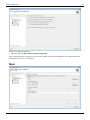
More Help
• Readers who are unfamiliar with Eclipse or the DESTECS tool are advised to read the overview first, before
starting this getting started section.
• If you encounter terms specific for the DESTECS tool that you are unfamiliar with, check the Glossary for their
meaning.
• An good introduction into 20-sim can be found in the 20-sim Getting Started manual
• A good introduction into VDM can be found here
[2]
.
[3]
.
Installing
• Install the DESTECS tool.
• Download the WaterTank model:
http:/ / www. destecs. org/ downloads/ Watertank. zip
[4]
• and store it on on any location where you have read and write access (e.g. My Documents). You do not have to
extract this zip-file.
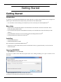
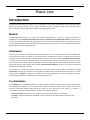
Opening DESTECS
• Open DESTECS from the start menu.
You will see a splash screen when the program opens and a dialog prompting you to give a location for the
workspace.
• Enter a location where you have read and write access.
The program should respond by opening with a welcome screen.
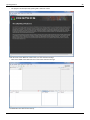
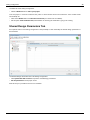
Getting Started
Click the Cross
Now the window should look like:
4
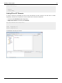
Getting Started
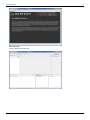
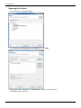
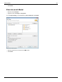
Opening the Project
• From the File menu choose File - Import.
• Select General and Existing Projects into Workspace and click Next.
• Select Archive File and Browse for the Watertank.zip file that you have downloaded.
• Click Finish to import the project.
5
Getting Started
6
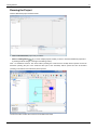
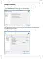
Running the Project
Now the Watertank project should be visibe.
• Click on the Watertank project entry to select it.
• Press the Debug button
. (if you have multiple projects loaded, you have to select the Watertank project first,
by clicking the black triangle at the right of the Debug button)
Now a co-simulation will start. The 20-sim editor (showing the continuous-time model) will be opened, the 20-sim
Simulator (showing the plot of the continuous-time part of the simulation) will be opened and the 3D animator
(showing an animation of the watertank) will be opened.
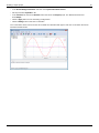
The 20-sim Editor contains the continuous-time WaterTank model.
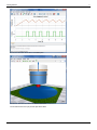
Getting Started
The 20-sim Simulator shows the co-simulated plots.
20-sim can also show simulation results in an animation.
The animation will start to play and the plot will be filled.
7
Getting Started
References
[1]
[2]
[3]
[4]
http:/ / youtu. be/ a0VaqWoYPT8
http:/ / www. 20sim. com/ downloads/ files/ 20sim42GettingStartedManual. pdf
http:/ / wiki. overturetool. org/ images/ 5/ 5b/ VDMSLGuideToOvertureV1. pdf
http:/ / www. destecs. org/ downloads/ Watertank. zip
Building a simple project
We will now create a project completely from scratch.
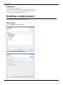
New Project
From the File Menu click New - Project
• Select DESTECS Project and click Next.
8
Building a simple project
• Enter the project name Simple and click Finish.
System Description
We wil create a VDM model and a 20-sim and run a co-simulation. The 20-sim model will run the following equation:
x = sin(time);
The equation runs in continuous time and exports the variable x though the DESTECS tool to the VDM model. In the
VDM model the following equation runs in discete-time:
y = amplitude*x;
It is updated every 100 ms. The variable y is exported back to 20-sim.
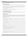
The Discrete Event Model
The overall structure of the discrete model is shown in the figure below. The System class contains the discrete-time
equation in association with the World class.
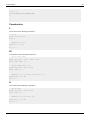
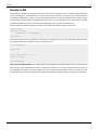
The Process Class
The process class defines the the two variables x and y which are needed to for the function calculateY which
calculates the function y = amplitude * x and prints the results to a log file. The active behaviour of the process is
modelled in the thread part of the class. The function calculateY is calculated every 100 ms. and will be running as
long as the simulation is in process.
class Process
values
public amplitude : real = 0.0;
instance variables
y : real := 0.0;
x : real := 0.0;
operations
public calculateY : () ==> ()
calculateY() ==
(
IO`print("Amplitude: "); IO`println(amplitude);
IO`print("x: "); IO`println(x);
IO`print("y: "); IO`println(y);
y := amplitude * x;
);
thread
periodic(100E6,0,0,0)(calculateY)
end Process
9
Building a simple project
• Copy the contents above and store in a text file called Process.vdmrt.
The System Class
The System class contains a reference to the Process class. As it can be seen in the instance variable section, the
modelled elements is referenced through the variable: p. The system class is responsible for deploying and allocating
the components in processing units called CPUs. This is the reason why an instance of the class CPU is declared.
system System
instance variables
public static p : Process := new Process();
-- Architecture definition
cpu : CPU := new CPU(<FP>, 20E3);
-- TODO Define deployable objects as static instance variables
operations
public System : () ==> System
System () ==
(
cpu.deploy(p,"process");
);
end System
• Copy the contents above and store in a text file called System.vdmrt.
The World Class
The World class is responsible for launching the simulation. This is done by invoking the start statement. This
operation will start the thread contained in the class, which models the active behaviour of the class.
class World
operations
public run : () ==> ()
run() ==
(
start(System`p);
block();
);
operations
block : () ==>()
block()==skip;
10
Building a simple project
sync
per block => false;
end World
• Copy the contents above and store in a text file called World.vdmrt.
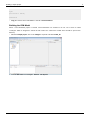
Building the VDM Model
When a new DESTECS project is created, several directories are created on its root, one of them is called
"model_de" which is designed to contain the DE model. The "vdmrt" files created above should be put into this
directory.
• Select the Simple project, click on the triangle to expand it and select model_de.
• From the File menu choose Import - General - File System.
11
Building a simple project
• Select the directory where you have stored the .vdmrt files.
• Select the three files and click Finish.
After adding the files to the directory, an error will be appear because the library "IO" used in the "Process" class is
not present.
• To add this library, right click the DESTECS project and press "Add DESTECS Library".
• The "Add Library Wizard" window will pop up. Select the "IO" library and press "Finish".
12
Building a simple project
At this point the "IO" library was added to your DE model and the model is ready to run, not displaying any error.
The Continuous Time Model
Modelling
We will build the continuous time model in 20-sim.
• From the Windows start menu open 20-sim.
• From the File menu select New - Equation Model.
• Enter the equations below.
parameters
real global amplitude ('shared');
externals
real global export x;
real global import y;
variables
real result;
code
// THE EXPORT FOR THIS MODEL
x =sin(time);
// IN BETWEEN HERE THE VDM/DESTECS WILL CALCULATE THE NEW VALUE:
// y = amplitude * x;
// AND IMPORT THE RESULT
result = y;
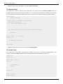
The model has one parameter that is shared with VDM. Two variables are exported (x) to VDM and imported (y) from
VDM. The code block describes the equation that is calculated. Now in 20-sim the result should look like the figure
below.
13
Building a simple project
Simulation
• Click on the Model menu and select Start Simulator.
Now a Simulator window will open.
In the Simulator click on the Properties menu and select Plot to open the Plot Properties.
• Select the variable x for the first curve.
• Choose Add Curve and select the variable y for the second curve.
• Close the Plot Properties.
• Run a simulation (click the Simulation menu and select Run).
14
Building a simple project
The result should look like:
The simulation shows the continuous-time equation x = sim(time), but the variable y is zero. This is obvious, because
have not coupled VDM yet.
• Return to the 20-sim Editor.
• Click on the File menu and select Save As and store the 20-sim model using the name simple.emx.
• In the 20-sim Editor from the File menu select Save.
• Save the model as simple.emx in the same location as the .vdmrt files.
Adding the 20-sim Model
Now we will add the 20-sim model to the project.
• Return to the DESTECS tool.
• In the tree from the Simple project select model_ct.
• From the File menu select Import - General - File System and click Next.
• Select the proper location (From Directory), select the 20-sim model simple.emx and click Finish.
Contract
We will continue by creating a contract that connects both the discrete-time and continuous-time model.
• In the tree select Simple.
• From the right mouse menu choose New-DESTECS'new contract and click 'Finish.
• Replace the contents of this file by the text below:
-- Shared Design Parameters
sdp real amplitude;
-- Monitored variables
monitored real x;
-- Controlled variables
15
Building a simple project
controlled real y;
-- Events
-- event HIGH;
Linking DE and CT Elements
In order to show the co-simulation tool how to link the elements from the contract to the DE and CT models
respectively a link-file must be present for each co-model. This is stored in a vdm.link file.
• In the tree select vdm.link (Simple\configuration)
• Replace the contents of this file by the text below:
sdp amplitude=Process.amplitude;
input
x=System.p.x;
output y=System.p.y;
The DESTECS tool will now look like:
16
Building a simple project
Debug Configuration
Before starting a co-simulation, a debug configuration must be created. The purpose of this is to define where the
continuous time and discrete event models are located, as well as the scenario file and the simulation time.
• Press the small arrow next to the debug icon
at the top of the workbench.
• A drop-down menu will appear, in which the option Debug configurations ... has to be selected.
• Select the option Co-Sim Launch and New launch configuration.
Now a window will show up where you can enter the settings of the Debug Configuration. We wil describe the tabs
that are necessary to run a co-simulation.
• Create a New Debug Configurationnamed Simple.
• In the Main tab change the settings (use the Browse buttons and set the time to 10s) until it looks like:
17
Building a simple project
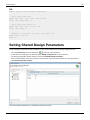
• In the Shared Design Parameters Tab click on the Synchronize with contract
• Set the parameter amplitude to 10.
• In the Common Tab click on the Browse button and choose the Simple project. The Shared file should now
show\Simple
• Click the Apply button to store the Debug Configurations.
• Click the Debug button to start the co-simulation.
The co-simulation will now start and the 20-sim Editor and Simulator will appear. After the co-simulation the 20-sim
Simulator should look like.
18
Movies
19
Movies
Click on the folllowing link to see the movies:
• How to open Destecs and run projects
[1]
.
Example Models
WaterTank
• Description: This is a model of a watertank showing the a basic co-simulation.
• More Information: The topic Getting Started shows you how to load and run the WaterTank model. More
information on the model itself can be found in the WaterTank topic.
• Download Location: http:/ / www. destecs. org/ downloads/ Watertank. zip
[4]
Simple
• Description: This is the Destecs version of "Hello World". A very simple model that you can create yourself and
run a co-simulation.
• More Information: The topic Building a Simple Project shows you how you create this model and run it.
• Download Location: http:/ / www. destecs. org/ downloads/ Simple. zip
[1]
Examples Compendium
• Description: The examples compendium contains a number of example projects. You can import these projects
using the zip file below.
More Information: More information on the examples can be found in: http:/ / www. destecs. org/ downloads/
examples_compendium_M33. pdf
[2]
Download Location: http:/ / www. destecs. org/ downloads/ examples_compendium_M33. zip
References
[1] http:/ / www. destecs. org/ downloads/ Simple. zip
[2] http:/ / www. destecs. org/ downloads/ examples_compendium_M33. pdf
[3] http:/ / www. destecs. org/ downloads/ examples_compendium_M33. zip
[3]
20
Basic Use
Introduction
The DESTECS tool allows you to define and a co-simulation. To get a basic understanding of the tool we first need to
define some concepts. We will use use a popular description of these concepts that might not be completely correct
but will, hopefully, enhance the understanding of beginning DESTECS users.
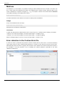
Models
It starts with models. Models are a more or less abstract representation of a system or component of interest. In
DESTECS we use continuous time-models (CT model) and discrete-event models (DE models). Continuous time
models are models that describe real physical systems. These models describe the behaviour of physical systems at
any desired time. Discrete-event models typically describe computer systems that run at a predetermined time steps.
Between these time steps nothing happens.
Simulation
Continuous-time models can be entered and simulated in 20-sim. This tool will calculate continuous-time models with
as many small time steps as required to get accurate results. Sometime the accuracy is violated. The tool will then
step back and use smaller time steps until the required accuracy is met. This is called a continuous-time simulation.
A continuous-time simulation is therefore always characterized by the accuracy of the simulation and the time steps
taken. Discrete-event models can be entered and simulated in VDM. This tool will calculate discrete-event models
with exactly the time steps required. This is called a discrete-event simulation. There is not accuracy involved and
therefore no backstepping is required.
The properties of a model that affects its behaviour, but which remains constant during a simulation are called
parameters. Examples of parameters are the height of a watertank with varying waterlevel or the mass of a car with
varying speed. A variable is a property of a model that may change during a given simulation. Examples of variables
are the varying waterlevel of a watertank or the varying speed of a car.
Co-Simulation
A co-simulation is a combined simulation of a continuous-time model and a discrete-event model in separate tools.
The DETSECS tool allows you to run discrete-event models in VDM and continuous-time models in 20-sim and
exchange information between VDM and 20-sim during run time. Because the the notion of a model in a
co-simulation may lead to misinterpretations, we will use the following definitions:
• constituent model: the continuous-time model or the discrete-event model of a co-simulation.
• co-model: a model comprising two constituent models (a discrete event submodel and a continuous-time
submodel).
Introduction
Contract
The description of the communication between the constituent models of a co-model is called the contract. A contract
typically describes the variables that are shared between the continuous-time model and the discrete-event model. An
example of a shared variable is the waterlevel that is calculated in the continuous-time model and sent to the
discrete-event model where it is used to calculate the response of a water level controller.
In most cases a continuous-time model and a discrete-event model will use similar parameters. For the watertank
example such a parameter may be the maximum water level. In the continuous time model this parameter indicates
the height at which a sensor is placed and in the discrete time model this parameter may indicate a property of the
water level controller. To prevent different values to be used in the continuous-time model and discrete-event model,
we may share this parameter in the contract. This is called a shared design parameter.
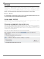
Opening Destecs
When you open the DESTECS tool for the first time, you will have to set the default location of your projects and
remove the welcome screen.
• Open DESTECS from the start menu or, go to the location where you have installed the DESTECS tool (e.g.
where you have extracted the zip file: ....\DestecsIde-versionid-win32.win32.x86\DestecsIde-versionid) and open
the the file Destecs.exe.
• You will see a splash screen when the program opens.
The splash screen shows that the DESTECS tool is opening.
• The first time the program is started you will have to decide where you want the default place for your projects to
be.
Choose the location of the workspace.
21
Opening Destecs
• The program should respond by opening with a welcome screen.
Click the Cross of the Welcome screen when you have read the message.
• Click on the cross of the Welcome tab to remove the welcome message.
The DESTECS tool after the first start-up.
22
The Destecs Tool
The Destecs Tool
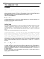
Workbench
Eclipse is an open source platform based around a workbench that provides a common look and feel to a large
collection of extension products. Thus, if a user is familiar with one Eclipse product, it will generally be easy to start
using a different product on the same workbench. The Eclipse workbench consists of several panels known as
views. A collection of panels is called a perspective. The figure below shows the standard DESTECS perspective. The
DESTECS perspective consists of a set of views for managing DESTECS projects and viewing and editing files in a
project. Different perspectives are available in DESTECS based on the task that you are doing.
Outline of the DESTECS Workbench.
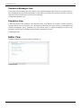
Explorer View
The DESTECS Explorer view lets you create, select, and delete DESTECS projects and navigate between the files in
these projects, as well as adding new files to existing projects.
The DESTECS Explorer view.
Outline View
The Outline view, on the right hand side of the figure above, presents an outline of the file selected in the editor. This
view displays any declared VDM definitions such as their state components, values, types, functions and operations.
The type of the definitions are also shown in the outline view. The Outline view is at the moment only available for the
VDM models of the system. In the case another type of file is selected, the message An outline is not available will be
displayed.
The class outline view showing the composition of the system VDM-RT class.
The colour of the icons in front of a name in the outline names indicates the accessibility of the corresponding
definition. Red is used for private definitions, yellow for protected definitions and finally green is used for public
definitions. Triangles are used for type definitions, small squares are used for values, state components and instance
variables, functions and operations are represented by larger circles and squares, permission predicates are shown
with small lock symbols and finally traces are shown with a “T”. Functions have a small “F” lifted over the icons and
static definitions have a small “S” lifted over the icon. For record types a small arrow is placed in front of the icon and
if that is clicked the fields of the records can be shown. In the case a System class is being displayed in the Outline
View, the root element representing the class will be a violet filled circle with an S in the center as illustrated in the
figure below.
Simulation Engine View
The Simulation Engine View, located in the lower left part of the environment is showing the evolution of a
co-simulation. This is done by monitoring the interaction between the VDM-RT discrete event simulation, the 20-sim
continuous time simulation and the engine. This view has two columns, the first one is specifying the source of the
message and the second one the content of it. As it can be seen in teh figure below, the values for the sources can be
All, VDM-RT or 20-sim. In
the first case, the message is common to both simulations. In the second case, the message belongs specifically to
either the discrete or the continuous simulation.
The engine view.
23
The Destecs Tool
Simulation Messages View
To the right of the Simulation Engine View, there is a view called the Simulation Messages View (see figure below). In
this case different messages coming specifically from the continuous or the discrete simulation are shown. Each entry
shows the source of the message, its content and a timestamp.
The Simulation Message view.
Simulation View
A third view related to the simulation is the Simulation View, which displays the evolution of certain parameters
specially relevant in the co-simulation. As in the Simulation Messages View, every message is timestamped and
ordered chronologically. This is illustrated in the figure below. There is a default arrangement of views in the
perspective, but they can be changed and then restored to the default at any time.
The Simulation view.
Editor View
The Editor View allows you to edit Contracts, Scenario's etc.
The Editor View.
24
Projects
Projects
All data that is necessary for a co-simulation (e.g. models, contracts etc.) is stored in a DESTECS project. This
section explains how to use the DESTECS tool to manage projects. Step by step instructions for importing, exporting
and creating projects will be given.
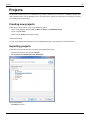
Creating new projects
Follow these steps in order to create a new DESTECS project:
• Create a new project by choosing File and New and Project and DESTECS project.
• Type in a project name.
• Click the button Finish (see the figure below).
Create project dialog.
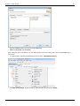
You can create projects in the DESTECS tool. The highlighted project is the project that is currently selected.
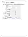
Importing projects
Follow these steps in order to import an already existing DESTECS project.
• Right-click the explorer view and select Import.
• Select General - Existing Projects into Workspace.
Import project dialog.
• Click Next to proceed.
25
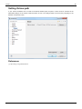
Projects
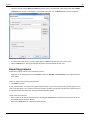
• Select the the radio button Select root directory if the project is uncompressed. Select the the radio button Select
archive file if the project is contained in a compressed archive file. Use the Browse button to locate the project.
Select project archive file.
• A compressed archive file may contain multiple projects. Select the projects that you want to import.
• Click the Finish button. The imported project will appear on the DESTECS explorer view.
Exporting projects
Follow these steps in order to export a DESTECS project:
• Right click on the target project and select Export, followed by General and Archive File. See the figure below for
more details.
Select an output format for the exporting process.
• Click Next to proceed.
A new window like the one shown in the figure below will follow. In this case the selected project will appear as root
node on the left side of it. It is possible to browse through the contents of the project and select the convenient files to
be exported. All the files contained in the project will be selected by default. Project ready to be exported.
• Enter a name for the archive file in the text box following To archive file. An specific path to place the final file can
be selected through the button Browse.
• Click on the Finish button to complete the export process.
26
Adding Models
Adding Models
When you have created a new project, you have to define the continuous-time model and the discrete-event model
that have to be coupled in a co-simulation.
Continuous-time model
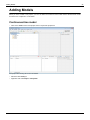
• Click on the arrow in front of the project name to expand the project tree.
The project tree showing the CT and DT entries.
• Select the item model_ct.
• Right-click and select Import - File System
27
Adding Models
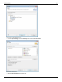
Import files into the DESTECS tool.
• From the Import Dialog, choose the directory that contains the 20-sim model.
Choose the file to import.
• Select the 20-sim model from the list of files.
28
Adding Models
• Click Finish.
Discrete-event Model
• Select the item model_de
• Right-click and select Import - File System. From the Import Dialog, choose the directory that contains the VDM model.
Choose the file to import.
• Select the directories that comprise the VDM 'model'.
• Click Finish
29
Contracts
Contracts
To connect the continuous-time model and discrete-event model together we have to define a contract.
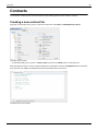
Creating a new contract file
Right click on the project that is going to contain the contract file. Select New and DESTECS new contract.
Choosing a new contract.
• A new window will pop up. Choose a contract name and click on the Finish button to end the process.
After following these steps a new file named projectName.csc will appear under the configuration folder contained in
the project tree. The middle of the Workbench will show the Editor with a new contract.
The Editor with a new contract.
30
Contracts
Contents of a Contract
A contract between a CT and a DE model can contain the following kind of information:
• Design parameters: These are typically values which indicate the properties of components (e.g. size, weight,
temperature). A designer would like to explore different values of these parameters in order to find an optimal
solution to the challenge he is working on. The actual values for the shared design parameters are set outside the
contract in a separate file.
• Variables: The variables are the active interface between the CT and DE models so these indicate the variables
that change during one simulation. Variables typically represent sensor readings and signals to actuators.
• Events: Events can be triggered in the CT world. They will stop the simulation before the allowed time slice is
completed. The co-simulation engine will then allow the DE simulator to take action but only until the point where
the event has been raised. The events are used in the contract in order to support event-based triggering and not
just time-triggered scheduling.
The syntax for contracts follow the following rules:
contract = parameters | variables | events ;
parameters =
‘shared_design_parameter’ type identifier ‘;’
| ‘sdp’ type identifier ‘;’
;
variables =
kind type identifier ‘;’
| kind 'matrix' identifier shape ';'
;
shape = '[' integer (',' integer)* ']' ;
events = ‘event’, identifier, ‘;’ ;
type = ‘real’ | ‘bool’ ;
identifier = initial_letter (following letter)* ;
kind = ‘monitored’ | ‘controlled’ ;
value = float | boolean_literal ;
boolean literal = ‘true’ | ‘false’ ;
In the following listing, an extract from the contract file provided with the WaterTank example is shown.
sdp real maxlevel;
sdp real minlevel;
monitored real level;
controlled bool valve;
31
Contracts
Matrixes
From Release 1.2.0 and onwards, it is possible to exchange matrices between DE and CT models. To be able to do
this, a matrix needs to be declared in the contract. The adopted syntax is similar to 20-sim, where the shape of the
matrix is indicated by a sequence of integers [m1,...,mn]. For example, to declare a 2x2 matrix which is monitored
named M the following must be added to the contract:
monitored matrix M[2,2];
For further information on how matrices are used in co-models, please see Matrices.
Arrays
Arrays can be declared in the same style:
monitored array position[3];
Although arrays are limited to one dimension.
Clarification
In VDM, even though both are represented in vdm as "seq of seq of real", a matrix[1,6] and a matrix[6,1] are distinct.
-matrix[1,3] - the outer seq has length 1, the inner seq has length 3 - example: [[1,2,3]]
-matrix[3,1] - the outer seq has length 3, the inner seq has length 1 - example: [[1],[2],[3]]
While a matrix[3]/array[3] is in fact just a "seq of real" with length 3 - example: [1,2,3]
Error detection in the Contract/Link file
A static error check is performed every time the contract or the link file are saved. This is a cross-file consistency
check which resolves if all the variables/events declared in a contract are also present in the link and vice-versa.
DESTECS will prevent the launch of projects with consistency errors between the contract and link files but there is
the possibility to turn this protection off by un-checking the referent preference (accessible in the menu
"Windows->Preferences") .
32
Contracts
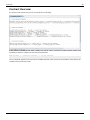
Contract Overview
An overview of the contract can be seen on the last tab of multi-editor.
In this view it is possible to see which variable from the DE side is connected to which contract variable and
transitively to which CT variable. The form they are presented is:
VDM variable <-> Contract Variable <-> 20-sim variable
The "not checked" appears next to the 20-sim variables because at this moment is not possible to static check if the
variables exist in the 20-sim model.
33
Linking DE and CT Elements
Linking DE and CT Elements
In order to show the co-simulation tool how to link the elements from the contract to the DE and CT models
respectively a link-file must be present for each co-model. This is stored in a vdm.link file.
DE model
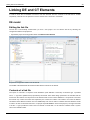
Editing the link file
The link file is automatically created when you start a new project. You can edit the link file by selecting the
configuration folder in the project tree.
• Expand the project and configuration folder and select the file vdm.link.
Expand the configuration folder to see the link file.
The middle of the Workbench will show the Editor with the contents of the link file.
Contents of a link file
The syntax of a link file is a sequence of link definitions (each definition is formed by an interface type, a qualified
name, “=” sign and a qualified name) separated by line breaks. Here all the design parameters, the variables and the
events from the contract must be present on the left-hand-side of each of these definitions. It is important to note that
the link file may contain more links than required by the contract, this allows a DE model to be reused in different
simulations where different contracts are used. Additionally, links can be made to variables that exist within the model
in order to be able to reference them from a script (the keyword model is used for this purpose). The right-hand-side
of all the “=” signs provide the names seen from the DE co-model side, f.e. the instance variables inside a system
class in the VDM-RT model.
34
Linking DE and CT Elements
The syntax of these definitions are:
vdmlink file = { interface, qualified name, ‘=’, qualified name, ‘;’ } ;
interface = ‘output’ | ‘input’ | ‘sdp’ | ‘event’ | ‘model’ ;
qualified name = identifier, [ ‘.’, identifier ] ;
identifier = initial letter, { following letter } ;
Link file parts
• input - links one monitored variable in the contract with a instance variable in the DE model. The qualified name
must start with the system class name.
• output - links one controlled variable in the contract with a instance variable in the DE model. The qualified name
must start with the system class name.
• sdp - links a shared design parameter in the contract with a value in the DE model. The qualified name can start
by any class name and the referenced value must be a "value" in VDM.
• model - links a "name" and a variable in the VDM model. The name can then be used to reference the variable in
scripts. The qualified name must start with the system class name.
The vdm.link file for the WaterTank example looks as:
input level=System.levelSensor.level;
output valve=System.valveActuator.valveState;
sdp maxlevel=Controller.maxLevel;
sdp minlevel=Controller.minLevel;
-- other linked names used in scenarios
model fault=System.levelSensor.fault;
CT Model
On the 20-sim side, a link file is not used, but still, the variables/parameters need to be declared in a certain way in
order to carry out the co-simulation.
Co-simulation variables
Variables used in the co-simulation, need to be in the 'externals' field and marked as 'global'. Depending if they are
used as input or output they need to be marked 'import' or 'export' respectively.
Example:
externals
real global export level;
real global import valve;
35
Linking DE and CT Elements
Shared Design Parameters
The parameters to be shared across the two models need to be marked with the keyword 'shared'.
Example:
parameters
real aParam ('shared') = 5;
Events
Events need to be marked using the keyword 'event', this marks the variable that it used as return value of the event
function to be an event variable. The keywords 'eventdown' and 'eventup' are used as in standalone 20-sim models.
See more under Events.
Example:
variables
boolean minLevelReached ('event');
equations
maxLevelReached = eventup(levelIn-maxlevel);
Debug Configuration
Before starting a co-simulation, a debug configuration must be created. The purpose of this is to define where the
continuous time and discrete event models are located, as well as the scenario file and the simulation time.
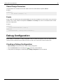
Creating a Debug Configuration
• Select the project for which you want t create a Debug Configuration.
• Press the small arrow next to the debug icon
at the top of the workbench.
• A drop-down menu will appear, in which the option Debug configuration has to be selected.
36
Debug Configuration
Select a new debug configuration.
• Select the option Co-Sim Launch and New_Configuration
Now a window will show up where you can enter the settings of the Debug Configuration. We wil describe the tabs
that are necessary to run a co-simulation.
Main
37
Debug Configuration
The Main tab of the Debug Configuration.
• Click the Browse button to select your project.
Once the project is found and selected, the paths for both Discrete Event and Continuous Time models will be
automatically set
• Click on the Browse button to select the scenario file (if a scenario file is available).
• Set the option Total simulation time, which defines for how long the simulation is going to be running.
Shared Design Parameters Tab
An important feature of the debug configuration is the possibility to view and modify the shared design parameters of
the simulation.
The Shared Design Parameters tab of the Debug Configuration.
• Click Synchronize with contract to import the shared design parameters.
• Set the parameters to their proper values.
After this step, it is possible to launch a Co-simulation.
38
Launching a Co-Simulation
39
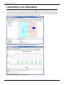
Launching a Co-Simulation
To start up a co-simulation you simply press the Debug button
. The 20-sim editor (showing the continuous-time
model) and the 20-sim simulation (showing the plot of the continuous-time part of the simulation) will be loaded
automatically. The simulation plot will show the variables during a simulation. If a 3D model of the system has been
developed for the CT model, an extra window with a 3D animator will also open.
The 20-sim Editor contains the continuous-time WaterTank model.
The 20-sim Simulator shows the co-simulated plots.
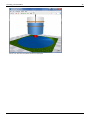
Launching a Co-Simulation
20-sim can also show simulation results in an animation.
40
41
Advanced Topics
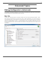
Debug Configuration (Advanced)
An introduction to the Debug Configurations was first made in the introductory part of this manual. In this section all
the tabs presented in the Debug Configuration will be introduced.
Main Tab
The Main Tab is where the project to co-simulate is selected. This can be done by pressing the "Browse..." button.
After selecting the wanted project (in the picture the project is called LineFollowACA_121), the DE model path is
automatically filled since it is only possible to have one DE model in the "model_de" folder. Though he CT model path
needs to be selected "Browse..." button. If a scenario should be used, it is possible to select which one in the
Simulation Configuration section. The total simulation time should be a number greater than zero to be able to run the
co-simulation.
Debug Configuration (Advanced)
Shared Design Parameters Tab
In the Shared Design Parameters tab, a list of the parameters used in the simulation can be viewed. For the variables
to appear for the first time the the button Synchronize with contract needs to be pressed. Every time the shared
design parameters are changed in the contract, the button must be pressed again in order to synchronize the view
with the contract.
For the variables present in the table it is possible to decide which values they will have when the co-simulation starts.
The following image shows the Shared Design Parameters tab for a project that has a matrix (2x2) has a shared
design parameter.
42
Debug Configuration (Advanced)
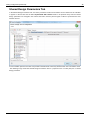
VDM Options Tab
The VDM Options tab is the tab where runtime options for the DE part of the model can be activated/deactivated. It is
divided in 4 options groups:
• Interpreting - these are options related with the interpretation of the DE models. Certain checks and also the
generation of reports such as coverage or the real-time events can be turned on/off;
• Log - in this section it is possible to select variables from the DE model that should be logged during the simulation.
To find more details about this feature, see Logfiles;*Faults - (experimental feature) in this section it is possible to
chose a class A to replace a class B before the simulation start; the intention is to experiment with faulty modules
that can be substituted by the non-faulty model. To make sure there will be no runtime exceptions, class B should
be subclass of A. To indicate that class A should be substituted by class B, the following should be inserted in the
text box "A/B". It is possible to make several substitutions by separating the substitutions with a comma
"A/B,C/D,...
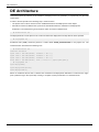
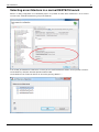
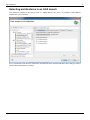
• Architecture - (experimental feature) in this section it is possible to select an architecture file that defines the
architecture of the deployment of the DE controller. More information on the architecture file can be seen in DE
Architecture
43
Debug Configuration (Advanced)
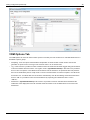
20-sim Options tab
The 20-sim Options tab contains options related with the execution of the CT model. At first, both tables (Log and
Settings) contain only the previously saved settings, if no settings were previously selected then the tables will be
empty; the tables can be populated by pressing the "Populate..." button. The "Populate..." button launches the model
selected in 20-sim model and dynamically extracts the settings and the variables present in the model. There is two
sections present in the 20-sim options tab:
• Log - in this section it is possible to select which CT variables should be logged during the co-simulation execution.
• Settings - the settings are presented in a tree view. In this tree there is two types of nodes, option nodes and
"virtual" nodes which are only there to give the tree structure. If an option node is selected, the different
possibilities will be presented on the right side ("Options" group).
44
Debug Configuration (Advanced)
In the picture above it is possible to see that two variables are selected for logging (top half of the tab). In the bottom
half it is possible to see that the 20-sim implementation of the "Control" (this is specific to the Watertank model) is
selected, the different submodels appear listed in the combo box in the right.
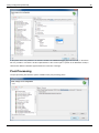
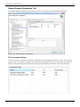
Post-Processing
The post processing tab shows the options available for the post-processing phase.
45
Debug Configuration (Advanced)
Octave Options
Show plot automatically when the script runs - with this option enabled, the Octave script that is generated after
each run will contain the commands to show the plot automatically, i.e., simply running the script will show the plots.
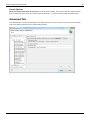
Advanced Tab
The advanced tab is reserved for developers, extra debug information can be turned on or off in this tab. More detail
on the extra debug information can be found in Debug Reports
46
Debug Configuration (Advanced)
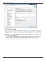
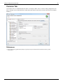
Common Tab
The Common tab is a standard Eclipse tab which, for example, allows users to save the debug configurations into
files so that they can be shared with others. More information about the tab can be found in the Common Tab Eclipse
website
[1]
.
References
[1] http:/ / help. eclipse. org/ galileo/ index. jsp?topic=/ org. eclipse. mtj. doc. user/ html/ reference/ launchers/ wireless_toolkit/
common. html
47
Scenarios
Scenarios
Introduction
Current version of DESTECS tool supports two different kinds of syntaxes for the script languages:
1. with the extension name ".script": For each project it is possible to define a large collection of scenarios. From a
discrete event perspective, these scenarios can be thought off as test cases. Each scenario can be considered as
a sequence of external stimuli to the co-simulation. Each stimulus has a time associated with it (that is when the
stimuli is injected into the simulation). In addition each stimulus has an action associated with it. Such actions can
set variables either at the CT or the DE side of the simulation.
2. with the extension name ".script2": this scripts allow users to define condition-action pairs (using a statement
called when), which perform an action when the condition becomes true during a co-simulation. This script allows
these conditions to reference the current co-simulation time and the state of the co-model, and to combine them
with logical operators. Actions can assign to selected parts of the co-model and also provide information back to
the user, as well as terminating the simulation.
This chapter topic describes how to create scenario files and introduces a command language for DESTECS scripts
called DCL (DESTECS Command Language). The main purpose of DCL is to allow engineers to simulate user input
and activate latent non-normative behaviours during a co-simulation. The language is designed to be sufficiently rich
as to allow engineers to influence a co-model during co-simulation, without being overly complex. For example, it
does not allow local variables to be defined.
Creating a new scenario file
Follow these steps in order to create a new scenario file:
• Right click on the project that is going to contain the contract file. Select New and DESTECS new scenario.
• A new window will pop up, named Scenario Wizard. Select the current project by clicking on the Browse button.
Click on the Finish button to end the process.
After following these steps a new file named Scenario.script will be placed under the scenarios folder. To use the
script2 functionality the extension of script file needs to be changed to "script2".
Scripts with extension name ".script"
The syntax of each scenario file needs to be:
scenario file = { numeric literal, (‘DE’ | ‘CT’), ‘.’, identifier, ‘:=’, symbolic literal }, ‘;’ ;
identifier = initial letter, { following letter } ;
symbolic literal = numeric literal | boolean literal | nil literal | character literal | text literal | quote literal ;
boolean literal = ‘true’ | ‘false’ ;
text literal = ‘ " ’, { ‘ \" ’ | character | escape sequence }, ‘ " ’ ;
quote literal = ‘<’, identifier, ‘>’ ;
In the following listing, an extract from the scenario file provided with the water tank introductory example is shown.
2.5 DE.fault := 2.33;
1.0 CT.Control\testSignal=1
Essentially the meaning of a scenario is simply that the indicated changes of the variables either on the DE or the CT
side is changing at the time (the first value in all cases) to the value provided after the “:=” sign. So these can be
48
Scenarios
considered as disturbances provided for the simulation at the specific time and thus each such a file correspond to
one scenario. Sweeping over for example different design parameters will be done with a kind of higher level scenario
as a part of the Design Space Exploration feature to be developed as a part of the DESTECS tool suite.
Scripts with extension name ".script2"
The syntax of each scenario file needs to be:
Script
script = top-level statement, [ { ‘;’, top-level statement } ], [ ‘;’ ] ;
Top-Level Statements
top-level statement = include statement | when statement | once statement;
include statement = ‘include’, ‘"’, file path, ‘"’ ;
when statement = ‘when’, expression, ['for' time literal], ‘do’, statement, [ ‘after’, revert block statement ];
once statement = ‘once’, expression, ['for' time literal], ‘do’, statement, [ ‘after’, revert block statement ];
Statements
statement = assign statement | print statement | error statement | ‘quit’ ;
revert block statement = ‘(’, revert statement, [ { ‘;’, revert statement } ], ‘;’ , ‘)’ ;
assign statement = identifier, ‘:=’, expression ';'
revert statement = ‘revert’, identifier ';'
print statement = ‘print’, formatted string ';'
error statement = ‘error’, formatted string ';'
Expressions
expression = boolean literal | numeric literal | time literal | ‘time’ | identifier | unary expression | binary expression ;
boolean literal = ‘true’ | ‘false’ ;
time literal = numeric literal, [ ‘{’, time unit, ‘}’ ] ;
time unit = ( ‘microseconds’ | ‘us’ ) | ( ‘milliseconds’ | ‘ms’ ) | ( ‘seconds’ | ‘s’ ) | ( ‘minutes’ | ‘m’ ) | ( ‘hours’ | ‘h’ ) ;
numeric literal = numeral, [ ‘.’, digit, { digit } ], [ exponent ] ;
exponent = ( ‘E’ | ‘e’ , [ ‘+’ | ‘-’ ], numeral) ;
numeral = digit, { digit } ;
identifier = domain, ('real' | 'bool') , identifier literal ;
domain = ‘de’ | ‘ct’ ;
unary expression = unary operator, expression ;
unary operator = ‘+’ | ‘-’ | ‘abs’ | ‘floor’ | ‘ceil’ ;
binary expression = expression, binary operator, expression ;
binary operator = ‘+’ | ‘-’ | ‘*’ | ‘/’ | ‘div’ | ‘mod’ | ‘<’ | ‘<=’ | ‘>’ | ‘>=’ | ‘=’ | ‘<>’ | ‘or’ | ‘and’ | ‘=>’ | ‘<=> ’ ;
formatted string = ‘"’, string, ‘"’, [ ‘%’, identifier, [ { ‘,’, identifier } ] ] ;
49
Scenarios
We assume that digit, string, and file path have their obvious definitions. Since no variables can be defined in the
script language, all identifiers will exist in the co-model and therefore identifier literal will conform to the conventions of
VDM and 20-sim.
Examples
The following introduces a series of simple examples that demonstrate the features of this script language.
when time = 5 do
(de real x := 10;);
The time keyword yields the current co-simulation time. The de keyword indicates that x is resides (at the top level) in
the DE model. Naturally, the ct keyword is used to indicate the CT model. Comments may also be included:
when time = 5 do
(ct real y := true;);
Statements can also be grouped in blocks (surrounded by parentheses and separated by semicolons) . Expressions
of time can optionally include a unit (e.g. milliseconds) given in curly braces. Units are assumed to be in seconds if no
unit is given. The engineer may output messages to the tool (or to a log in batch mode) with the print statement:
when time = 900 {ms} do
(
de real x := 10;
ct real y := true;
print "Co-simulation time reached 900 ms.";
);
Logical operators can be used in expressions. When the condition becomes true, the statement(s) in the do clause
will execute. If the condition becomes false again, the optional after clause will execute once. Note that block
statements do not permit local variables to be defined.
when time >= 10 and time < 15 do
(print "Co-simulation time reached 10 seconds.";)
Since this script language does not allow local variables to be defined, a special statement, revert, may be used in an
after clause to change a value back to what it was when the do clause executed.
when time >= 10 and time < 15 do
(
// assume x = 5
de real x := 10;
)
after
(revert de real x;);
50
Scenarios
The engineer can reference co-model state in conditions and assignment and revert statements. The state that can be
referred is wither for VDM specified with the model keyword in the link file or for 20-sim marked as global (note
20-sim access is not yet implemented). Additionally all shared variables can be accessed with the contract name and
used in conditions, assignments or revert statements.
It is also possible to have some statements executed exactly once, on the first time a condition is detected. This is
acheived using the once keyword instead of when.
once de real x >= 500 do
(
// set some flag
de bool flag = true;
print "First time x exceeds 500";
)
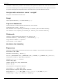
Logfiles
When starting a simulation, it is possible to select a set of variables that are logged throughout the co-simulation. At
the moment this manual is being written there is only the possibility of logging DE variables; support to log CT
variables will be added later. The result of this logging is a CSV file (comma separated values).
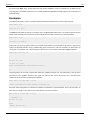
DE variables
The variables of the DE model to log can be selected in the tab VDM Options presented in the figure below. If a model
does not contain type errors, this tab will display all instance variables that are accessible from the VDM system class.
VDM Options tab permits the selection of variables to log.
51
Logfiles
Checking the box next to a variable enables the logging of that variable. Currently it is only possible to log variables
with basic types (all types except objects).
For the Watertank example, if we use the configuration shown above, a file with the contents as follows is generated:
time_,levelSensor.fault,levelSensor.level,valveActuator.valveState
0.0,0,0,0
0.01,0,0.01,0
0.01,0,0.02,0
0.02,0,0.03,0
0.03,0,0.03,0
... ... ... ...
The first column is the time and the following ones are the value of the variable at the given moment. A CSV file can
be better visualized, for example, in 20-sim, Excel or other software capable of opening this format.
Debug Reports
Once the simulation has been completed, a set of log files will be generated. The contents of these files are displayed
while the simulation is running in the simulation logging views. Even though those records are shown on the tool, it
might be useful to have them logged to external files for further post-simulation analysis.
The Engine.log file
The Engine.log file is registering the events indicated from the discrete event simulation, noted by VDM-RT in the
beginning of the entry, from the continuous simulation (indicated by 20-sim in the beginning of the entry) or both
(labelled All). As an example of an Engine log, an extract from the one generated after the WaterTank simulation is
shown below.
As it can be seen, it is registered how the engine has been loaded, which design parameters are going to be used and
the versions corresponding to the different continuous time and discrete event simulation applications. Paths to the
exact models and the loading actions together with their results are monitored as well.
All , Simulation engine type loaded:
org.destecs.core.simulationengine.ScenarioSimulationEngine
All , Shared Design Parameter initialized as:
(maxlevel:=0.0 minlevel:=0.0 )
VDM-RT , Launching
VDM-RT , Interface Version: name: VDMJ version: 0.0.0.1
VDM-RT , Initilized ok: true
20-Sim , Interface Version: name: 20-sim version: 4.1.2.3
20-Sim , Initilized ok: true
VDM-RT , Loading model:
C:\Users\ja\DestecsIde-0.0.2\workspace\watertank_new\model
52
Debug Reports
VDM-RT , Loading model completed with no errors: true
20-Sim , Loading model:
C:\Users\ja\DestecsIde-0.0.2\workspace\watertank_new\
watertank_new.emx
20-Sim , Loading model completed with no errors: true
VDM-RT , Interface => Design P( maxlevel minlevel )
Inputs( level ) Outputs( valve )
20-Sim , Interface => Design P( Control\maxlevel
Control\minlevel Control\testSignal )
Inputs( valve ) Outputs( level )
All , Validating interfaces...
All , Validating interfaces...completed
Once simulation time is over, the engine will send termination commands to each continuous and discrete
simulations. This is notified in a three stepped way, indicating that the process is going to be terminated, indicating
that the process has been sent the kill command and finally a done message. As it can be seen, the labels VDM-RT
and 20-sim are used to indicate whether the message is referring to the continuous time or the discrete event
simulation.
VDM-RT , Terminating...
VDM-RT , Terminating...kill
VDM-RT , Terminating...done
20-Sim , Terminating...
20-Sim , Terminating...kill
20-Sim , Terminating...done
The Message.log file
The Message.log file is logging the the messages coming from both VDM-RT discrete and20-sim continuous
simulation. In the following listing, the contents of the Message.log file for the water tank example are shown. Note
that that the structure this file is presenting is similar to the co-simulations run by the DESTECS tool. As it can be
seen, the first step is to check the version of the components so they can be initialized and loaded afterwards. The
next step is to query the interface for the simulation engine and set the appropriate design parameters. Once those
preliminary actions have been executed the simulation can be started.
VDM-RT , getVersion , 0.0
VDM-RT , initialize , 0.0
20-Sim , getVersion , 0.0
20-Sim , initialize , 0.0
VDM-RT , load , 0.0
20-Sim , load , 0.0
VDM-RT , queryInterface , 0.0
20-Sim , queryInterface , 0.0
VDM-RT , setDesignParameters , 0.0
VDM-RT , start , 0.0
20-Sim , start , 0.0
VDM-RT , step , 0.0
53
Debug Reports
As in the case of the Engine.log file the terminating signals are registered as well in the Message.log file. See the
listing below.
VDM-RT , stop , 10.0
VDM-RT , terminate , 10.0
20-Sim , terminate , 10.0
The Simulation.log file
The Simulation.log file is reflecting the evolution of the different parameters under study in a given co-simulation. In
the WaterTank example this is focused on the values of the variables level and valve and thus these are logged (see
listing below).
VDM-RT , valve=0.0 , 2.0
20-Sim , level=2.0 , 2.0
VDM-RT , valve=0.0 , 4.0
20-Sim , level=4.0 , 4.0
VDM-RT , valve=0.0 , 6.0
20-Sim , level=6.0 , 6.0
VDM-RT , valve=0.0 , 8.0
20-Sim , level=8.0 , 8.0
VDM-RT , valve=0.0 , 10.0
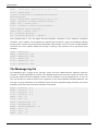
This is definitely a valuable collection of data, since it can be exported as data files for analysis by external tools.
Automated Co-model Analysis
In order to support Design Space Exploration (DSE), the Automated Co-model Analysis (ACA) is a feature that
enables running many different co-simulations with minimal user intervention. The ACA feature enables the user to
select different configurations for each individual parts of the co-model and then runs the co-simulation combining all
possible configurations that were selected by the user.
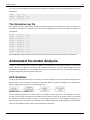
ACA Workflow
The figure below illustrates the steps in the process of the ACA work flow. First the user provides configurations for
different parts of the co-simulation, then the tool generates different complete configurations by composing the
different configurations parts that were provided by the user.
Illustration of the ACA process.
These complete configurations are used to execute co-simulations. At this stage, year 2 of the project, only the first
two part of the work flow are supported; year 3 will bring the automatic analysis of the results of these co-simulations
as well with presenting the results. Currently, it is only possible for the user to select different configurations for
different parts of the co-simulation, more specifically, chose different architectures for deployment of the controller (DE
side), and select different starting values for the shared design parameters.
54
Automated Co-model Analysis
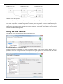
Illustration of the ACA process.
From these partial configurations it is possible to construct complete configurations in by combining each of the
different partial configurations. The figure above together with the following description helps illustrating the concept.
The result of generating complete configurations from the partial configuration would be 4 different complete
configurations: A1-B1-C1; A1-B1-C2; A1-B2-C1; and A1-B2-C2. The user can easily get many more configurations by
adding more parameters or adding more values to existing parameters, for example, simply adding a A2 value would
result in 4 more different configurations.
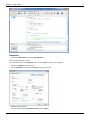
Using the ACA features
Launching an ACA is made through the Debug Configuration menu.
ACA Launch in the Debug Configuration Menu.
Creating a new Debug Configuration of an ACA Launch type will bring up the menu to configure the ACA. As it is
possible to notice from the figure below, the several present tabs ((The rightmost tab, the Common tab, will not be
mention here since is a standard Eclipse tab) will be explained individually in the following subsections.
55
Automated Co-model Analysis
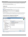
To start an ACA launch, a base configuration needs to be selected. This configuration is a normal DESTECS launch
which will be used as base for the ACA settings. This means that launch options that are not overwritten in the ACA
will use as default the ones present in the base launch.
There is also an Octave option which is explained in the Octave page.
The Main Tab
The Main tab will be the place where general settings for the ACA launch are set. Currently the only option present is
the Base Configuration. The Base Configuration, as the name says, is the configuration that forms the base for the
ACA to work.
ACA Launch - Main tab.
By pressing the button Browse it is possible to browse through the Co-Sim Launches present in the DESTECS Tool
and chose one. This configuration will be the base configuration for all the ones generated by the ACA. The ACA will
take the base configuration and combine it in all possible ways depending on what the user set on the other tabs.
The Architecture Tab - Deployment Architectures
It is possible in this tab to select which Controller Architectures will be used in the ACA run. For more information on
Controller Architectures and how to define them please see DE Architecture
ACA Launch - Architecture tab.
56
Automated Co-model Analysis
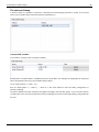
Shared Design Parameters Tab
In the Shared Design Parameters tab it is possible to make a value "sweep" of the shared design parameters.
ACA Launch - Shared Design Parameters tab.
The incremental Sweep
In the first column it is possible to select from a drop-down the shared design parameter to sweep. In the second
column (From), it is possible to select the value which the sweep should start from. The third column (To) indicates
where the sweep should end and the forth column (Increment By) indicates the increment to be used in the sweep.
57
Automated Co-model Analysis
The value set Sweep
In the first column it is possible to select from a drop-down the shared design parameter to sweep. In the second
column a list of double values should be introduced, separated by (;)
Complex SDP variables
It is possible to sweep by value set complex variables.
The behaviour of complex SDPs is a bit different from the atomic SDPs. For example, the configuration on the picture
above will generate 2 ACA runs for the variable "initial_Position".
1st run: initial_Position = [-1.448,-1.110]
2nd run: initial_Position = [-1.736,X*] - * where X is the value defined in the base debug configuration for
initional_Position[2].
The values defined in the value sweep are put together according to the order they appear, if a for one of the indexes
is missing (like in this case the second value of initial_Position[2]), the value from the original debug configuration will
be used.
58
Automated Co-model Analysis
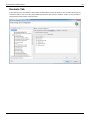
Scenario Tab
In the scenarios tab it is possible to select which scenarios will be used in the ACA run. The scenarios present in the
"scenarios" folder in the root of the project will be presented on the "Scenario selection" table. It is then possible to
check which scenarios will be used in the ACA.
59
Automated Co-model Analysis
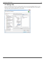
CT Settings Tab
The CT side settings here work much in a similar fashion to the ones in the normal DESTECS launch. The only
difference is that it is possible to select multiple options instead of one. In the ACA Settings tab it is only possible to
select options which have limited alternatives (i.e. enumerations).
60
Automated Co-model Analysis
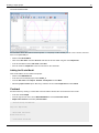
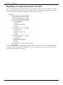
Repeating one single launch part of an ACA
After a successful ACA launch, the output folder will contain information regarding what was exactly run in a specific
ACA launch. This information in stored in the "output" folder. By looking closely at the figure below which shows the
result of an ACA run, it is possible to see a file named "xxx.dlaunch" for each ACA run.
By right-clicking a "dlaunch" file and selecting the option DESTECS-> Create and Launch, the single selected run will
be launched again. This single launch configuration is also stored together with the other launch configurations,
typically its name is prefixed by "generated".
61
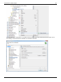
Automated Co-model Analysis
Inspecting the launch configurations it is possible to find the launch that was just created. The launch contains all the
same settings as the launch that was selected to be created from the ACA
62
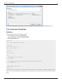
Control Library
Control Library
In order to help build controllers in VDM that can handle low-level proportional control in addition to supervisory
control, a control library has been included in the DESTECS tool. This library provides classes that are equivalent to
the P, PD, PI and PID blocks of the 20-sim library under Signal\Control\PID Control\Discrete.
Accessing the Control Library
To use the control library, the class definitions must be imported into the project.
• rightclick on the project and select New and Other....
• Under the DESTECS folder, select Add DESTECS Library and click Next.
Add the Control Library TODO: New screenshot with control library in.
• Then check the box marked Control Library.
Unless you want to edit the class files, leave Use linked libraries checked (default). The classes will now be added to
your co-model.
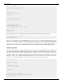
Using the Control Library
Basic Use
To use a class from the library, simply define a variable of the correct type, instantiate it with a constructor, call
SetSampleTime and then call Output in your control loop. All of the control library classes have an operation called
Output, which takes in an error and returns a control value, with the following form:
public Output: real ==> real
Output(err) == ...
<span class="Apple-style-span" style="line-height: 16px; ">
class Controller
instance variables
-- controller object
private pid: PID;
-- setpoint
private SP: real;
-- shared variables
private MV: real;
private out: real
operations
-- constructor for Controller
public Controller: () ==> Controller
Controller() ==
(
63
Control Library
pid := new PID(10, 1, 0.1);
pid.SetSampleTime(SAMPLE_TIME)
);
-- control loop
public Step: () ==> ()
Step() ==
(
dcl err: real := SP - MV;
out := pid.Output(err)
);
-- 100Hz control loop
values SAMPLE_TIME = 0.01;
thread periodic(10E6, 0, 0, 0)(Step);
end Controller
</span>
Also, all of the classes have an operation called SetSampleTime, which takes a sample time in seconds:
public SetSampleTime: real ==> ()
SetSampleTime(s) ==
Unlike 20-sim, VDM does not have a sampletime keyword, so it is necessary to explicitly tell the object what sample
time to use in calculations. Therefore, for all control objects (except P) you must call SetSampleTime before the
Output is used. This only needs to be done once and it is recommended that it is called immediately after the
constructor. If this is not done, the co-simulation will fail with a pre-condition violation the first time Output is called.
Advanced Use
All of the controller classes in the library are subclasses of a single class called DTObject (discrete-time object). This
class contains the definitions for SetSampleTime and Output and enforces a consistent interface. It is possible to use
the various controller classes without making reference to DTObject. However, if it is desirable to test different
controllers, variables can be defined as type DTObject, meaning that only the call to the constructor needs to be
changed in order to use a different controller implementation. This is also useful if control objects are passed to
controllers. In the following example, the Controller class can accept any control object (P, PID etc.):
class Controller
instance variables
-- controller object
private ctrl: DTControl;
operations
-- constructor for Controller
public Controller: DTControl ==> Controller
Controller(c) ==
64
Control Library
(
ctrl := c;
ctrl.SetSampleTime(SAMPLE_TIME)
);
...
Constructors
P
The P class has the following constructors:
-- set k
public P: real ==> P
P(k) == ...
-- default: k = 0.2
public P: () ==> P
P() == ...
PD
The PD class has the following constructors:
-- set k, tauD, beta
public PD: real * real * real ==> PD
PD(k, tauD, beta) == ...
-- set k, tauD, beta = 0.1
public PD: real * real ==> PD
PD(k, tauD) == ...
-- default: k = 0.2, tauD = 1.0, beta = 0.1
public PD: () ==> PD
PD() == ...
PI
The PI class has the following constructors:
-- set k, tauI
public PI: real * real ==> PI
PI(k, tauI) == ...
-- default: k = 0.2, tauI = 0.5
public PI: () ==> PI
PI() == ...
65
Control Library
PID
The PID class has the following constructors:
-- set k, tauI, tauD, beta
public PID: real * real * real * real ==> PID
PID(k, tauI, tauD, beta) == ...
-- set k, tauI, tauD, beta = 0.1
public PID: real * real * real ==> PID
PID(k, tauI, tauD) == ...
-- default: k = 0.2, tauI = 0.5, tauD = 0.5, beta = 0.1
public PID: () ==> PID
PID() == ...
Setting Shared Design Parameters
The shared design parameters that the simulation is using can be modified from the Debug configuration view.
• Press the small arrow next to the debug icon
at the top of the workbench.
• A drop-down menu will appear, in which the option Debug configurations has to be selected.
• The Dubug Configuration window will open. Click the tab Shared Design Parameters.
• A list of the parameters used in the simulation can be viewed. In the case the parameters are changed, click the
button Synchronize with contract.
The shared design parameter tab, in the Debug Configuration window.
66
Setting Shared Design Parameters
Setting Shared Design Parameters for batch execution
For command-line execution (planned in future versions of DESTECS) the design parameters that are shared
between the CT and DE models are placed in a separate file with a file extension called .sdp. These are typically
parameters that the user will wish to sweep over with multiple values. The syntax of the .sdp file needs to be:
sdp file = [ identifier, ‘=’, numeric literal ], ‘;’ ;
identifier = initial letter, { following letter } ;
Note that at the moment the only type of literals that may be used are numeric literals since 20-sim is limited to that.
Note also that the identifier must be defined both as a shared parameter inside the CT model as well as publicly
declared values inside the DE model as it is linked in the link-file. There is not yet any static check ensuring this but
this will be defined in the tools later.
Matrices
Matrices were introduced in the release 1.2.0.
Matrix Example
A simple example where a matrix (2x2) is transferred back and forward from DE to CT sides. The co-model does not
do anything else besides the transfer and a small calculation with the matrix This example called "example_matrix"
can be found in the examples zip distributed together with the release.
Contract
The matrices must be declared in the contract:
-- Shared Design Parameters
sdp real amplitude;
-- Monitored variables
monitored matrix x[2,2];
-- Controlled variables
controlled matrix y[2,2];
The matrix "x" is the output from 20-sim and the "y" is used as input for 20-sim. Both are declared with size 2x2.
20-sim
The 20-sim model is as simple as this one here:
parameters
real global amplitude ('shared') [2,2];
externals
real global export x[2,2];
real global import y[2,2];
variables
real result[2,2];
67
Matrices
68
code
// the export for this model
x = amplitude * [time, sin(time); cos(time), sin(time) * cos(time)];
// IN BETWEEN HERE THE VDM/DESTECS WILL CALCULATE THE NEW VALVE CONTROL VALUE
// and import the valveControl
result = y;
The matrices behave as any other variable that is being transmitted in DESTECS. In 20-sim the matrix notation is
used to both declare and operate over the matrices.
VDM
In VDM matrices of "n" dimensions (m1 x ... x mn) are represented as (seq of ... seq of real). So a 2x2 matrix is
represented as a (seq of seq of real).
The contract matrix variables are linked in the same manner as any other variable but the target variable needs to be
of the correct type, in our case seq of seq of real.
class Process
values
public amplitude : real = 0.0;
instance variables
y : seq of seq of real := [[0.0,0.0],[0.0,0.0]];
x : seq of seq of real := [[0.0,0.0],[0.0,0.0]];
operations
public calculateY : () ==> ()
calculateY() ==
(
IO`print("Amplitude: "); IO`println(amplitude);
IO`print("x: "); IO`println(x);
y := x;
);
thread
periodic(100E6,0,0,0)(calculateY)
end Process
DE Architecture
DE Architecture
This feature allows the selection of the hardware and deployment to be specified in a separate file from the VDM
system class.
In order to do this separation, the following steps need to be done:
• The System class must be cleaned of CPU and BUS declarations and deployments of the objects
• Annotations need to be added to the system class that indicate where the architecture and deployment
statements. The architecture tag must be places under an instance variables block:
-- ## Architecture ## -The deployment tab must be places in the constructor where the deployment normally will have been specified:
-- ## Deployment ## -Architecture files (.arch), should be placed in a folder called "model_de/architectures" in the project root. The
architecture files should have the following form:
-- ## Architecture ## -instance variables
cpu1: CPU := new CPU(<FCFS>, 1000000 /* Hz */);
cpu2: CPU := new CPU(<FCFS>, 1000000 /* Hz */);
cpu3: CPU := new CPU(<FCFS>, 1000000 /* Hz */);
bus1: BUS := new BUS(<FILO>, 1000 /* bits/s */,{cpu1,cpu2,cpu3});
-- ## Deployment ## -cpu1.deploy(mmi);
cpu3.deploy(navigation);
cpu2.deploy(radio);
When an architecture file like this is selected, the architecture and deployment declaration is inserted in the "right"
place (under the tags in the system file), creating a "complete" system just before the co-simulation starts.
69
DE Architecture
Selecting an architecture in a normal DESTECS launch
When in a debug configuration for a DESTECS project, it is possible to select which architecture is to be used at
run-time in the "Controller Architecture" group in the VDM Tab.
If the "model_de/architectures" folder does not exist yet, the "Create Architecture Folder" can be pressed to create it.
The architecture (.arch) files should be placed inside this folder.
The architecture to be used in the launch can be used by pressing "Browse...".
70
DE Architecture
Selecting architectures in an ACA launch
The architecture selection in the ACA is made in a slightly different way, since it is possible to select different
architectures to use in the ACA.
As it is characteristic of the ACA, the architectures selected here will be combined with all the other settings in order to
generate all the permutations of settings.
71
Events
72
Events
Events can be triggered in the CT world. They will stop the simulation before the allowed time slice is completed. The
co-simulation engine will then allow the DE simulator to take action but only until the point where the event has been
raised. The events are used in the contract in order to support event-based triggering and not just time-triggered
scheduling.
Simulation setup
Events in the contract
For events to be considered during a simulation the event must be defined in the contract:
events = ‘event’, identifier, ‘;’ ;
Events in the link file
Events must be connected to a public async operation in VDM. This is done by linking the event name specified in the
contract to the fully qualified operation name in VDM in the link file:
events = 'event', identifier = 'System', '.', identifier, ('.', identifier)+
Example:
event event1=System.eventHandler.event1;
Where:
• "event1" is the event name from the contract
• System is the system class
• eventHandler is the class holding the operation to execute
• "event1" (the last event1) is the async operation which to execute when the event occurs
Events in CT
Events need to be marked using the keyword 'event', this marks the variable that it used as return value of the event
function to be an event variable. The keywords 'eventdown' and 'eventup' are used as in standalone 20-sim models.
See more under Events.
Example:
variables
boolean minLevelReached ('event');
equations
maxLevelReached = eventup(levelIn-maxlevel);
Events
73
Events in DE
The scheduler in VDM do not schedule events in the same way as for instance a micro controller would do where the
current executing job is suspended in favour of the interrupt routine. However, it is possible to get a similar behaviour
by creating and deploying an object to a CPU that contains the job to run when an interrupt occurs and then call this
from the async operation which is triggered when event occurs. It is just important that no objects having a periodic
threads are deployed to the same CPU since this will delay the event by exactly one periodic loop.
Events are linked to VDM through async operations and made assessable through the system class.
system System
instance variables
eventHandler : EventHandler;
end System
The async operation must be specified in a class that is not deployed to a CPU. This makes the evaluation instant.
This means that the event operation it self do not take time to run.
class EventHandler
operations
public async event1: () ==> ()
event1()== skip;
end EventHandler
Note about the VDM scheduler: The VDM scheduler uses priorities to select which thread should run,each thread is
then executed with a limited allowed number of expressions/ statements it can execute before another thread has to
be schedulled and executed. The priority defined how many expressions/ statements a thread can execute at a time.
A thread will always continue executing until it is blocked or finished the allowed number of expressions/ statements.
Octave
Octave
GNU Octave is a high-level interpreted language, primarily intended for numerical computations. It provides
capabilities for the numerical solution of linear and non-linear problems, and for performing other numerical
experiments. It also provides extensive graphics capabilities for data visualization and manipulation. Octave is
normally used through its interactive command line interface, but it can also be used to write non-interactive
programs. The Octave language is quite similar to Matlab so that most programs are easily portable. [1]
Octave Version
It is very important that the correct version of Octave is used to run the scripts generated by DESTECS. The correct
version can be found in Chessforge together with the DESTECS Releases.
Octave use in DESTECS
After each co-simulation run, an Octave script is generated in the output dir. The script contains Octave code that
reads the variable logs produced by both VDM and 20-sim during the run.
Show plot automatically when script is run
There is one option available in the debug configuration that affects the script. This option appears in two places both
in the normal DESTECS run and in ACA. If enabled, when the script is executed, a plot (or several, depending on the
amount of variables selected) will automatically be drawn. In the case of an ACA run being executed, for the same
variable, the several runs will juxtaposed.
Picture below shows where to find this option for a normal run (Post-Processing tab).
And in the ACA launch (Main Tab)
74
Octave
Invoking Octave from DESTECS
It is possible to invoke Octave from the DESTECS IDE. Right-clicking on an Octave (.m) file reveals the option "Run
Octave". If you want to use this command, be sure to tick the "Show plot automatically when the script runs" box
If the tick to show plot automatically was checked, a plot will be drawn and shown in a window like this:
75
Octave
Setting Octave path
If your Octave installation was not made in the default installer path, the path to Octave must be corrected in the
DESTECS settings for the feature mentioned above to work. The settings below can be found by navigating to the
Window->Preferences menu.
References
[1] http:/ / www. gnu. org/ software/ octave/
76
Folder Launch Configuration
Folder Launch Configuration
This is a en EXPERIMENTAL feature. This is a new way of launching an ACA by selecting a folder containing
".launch" files. The user has to produce it's own ".launch" files. The options to select are the project and the folder
containing the launch files.
77
78
Additional Information
Syntax Notation
Wherever the syntax for parts of the language is presented in the document it will be described ina BNF dialect. The
BNF notation used employs the following special symbols:
,
the concatenate symbol
=
the define symbol
|
the definition separator symbol (alternatives)
[]
enclose optional syntactic items
{}
enclose syntactic items which may occur zero or more times
‘’
single quotes are used to enclose terminal symbols
meta
identifier
non-terminal symbols are written in lower-case letters (possibly including spaces)
;
terminator symbol to denote the end of a rule
()
used for grouping, e.g. “a, (b j c)” is equivalent to “a, b j a, c”.
–
denotes subtraction from a set of terminal symbols (e.g. “character – (‘ " ’)” denotes all characters excepting the double
quote character.)
Glossary
Glossary
As might be expected in such an interdisciplinary project, terms and concepts that are well known in one discipline
may be unknown or understood quite differently in another. This page therefore contains common descriptions of core
concepts agreed with the partners that are used consistently within the project.
A
• abstract class: (in object oriented programming) a class where one or more methods are defined abstractly using
the text "is subclass responsibility" as their body.
• actuator: a component that produces a physical output in response to a signal.
• aggregate: (in object oriented programming) the act of bringing together several objects into a single whole.
• automated co-model analysis: tool support for the selection of a single design from a set of design alternatives
(including definition of scenarios, execution of co-simulations, and visualisation and analysis of co-simulation
results).
B
• bond: (in bond graphs) a directed point-to-point connection between power ports on submodels. Represents the
sharing of both flow and effort by those ports.
• bond graph: a domain independent idealised physical model based on the representing energy and its exchange
between submodels.
C
• causality: (in bond graphs) dictates which variable of a power port is the input (cause) for sub-model’s equations
and which is the output (effect).
• class: (in object oriented programming) the definition of the data field and methods an object of that class will
contain.
• code generation: the process of implementing a system controller by automatically translating a model into a
representation (in some programming language) which can then be executed on the real hardware of the system.
• commit: to record changes to data under revision control.
• co-model: a model comprising two constituent models (a DE submodel and a CT submodel) and a contract
describing the communication between them.
• configuration management: the managing of the composition of co-models from various DE and CT models.
• consistency: a co-model is consistent if the constituent models are both syntactically and semantically consistent.
• constituent model: one of the two submodels in a co-model.
• continuous-time simulation : a form of simulation where ``the state of the system changes continuously through
time".
• contract : a description of the communication between the constituent models of a co-model, given in terms of
shared design parameters, shared variables, and common events.
• controlled variable : a variable that a controller changes in order to perform control actions.
• controller : the part of the system that controls the plant.
• controller architecture : the allocation of software processes to CPUs and the configuration of those CPUs over a
communications infrastructure.
• co-sim launch: the type of debug configuration used in the DESTECS tool to define and launch a single scenario.
• co-simulation baseline : the set of elements (co-model, scenario, test results etc.) required to reproduce a
specific co-simulation.
79
Glossary
• co-simulation engine : a program that supervises a co-simulation.
• co-simulation : the simulation of a co-model.
• cost function : a function which calculates the "cost" of a design.
D
• debug config:(Eclipse term) the place in Eclipse where a simulation scenario is defined.
• design alternatives : where two or more co-models represent different possible solutions to the same problem.
• design parameter : a property of a model that affects its behaviour, but which remains constant during a given
simulation.
• design space exploration : the (iterative) process of constructing co-models, performing co-simulations and
evaluating the results in order to select co-models for the next iteration.
• design step : a co-model which is considered to be a significant evolution of a previous co-model.
• discrete-event simulation : a form of simulation where ``only the points in time at which the state of the system
changes are represented.
• disturbance : a stimulus that tends to deflect the plant from desired behaviour.
E
• edges: (in bond graphs) see bond.
• effort: (in bond graphs) one of the variables exposed by a power port. Represents physical concepts such as
electrical voltage, mechanical force or hydraulic pressure.
• environment : everything that is outside of a given system.
• error : part of the system state that may lead to a failure.
• event : an action that is initiated in one constituent model of a co-model, which leads to an action in the other
constituent model.
• executable model : a model that can be simulated.
F
• failure : a system's delivered service deviates from specification.
• fault injection : the act of triggering faulty behaviour during simulation.
• fault modelling : the act of extending a model to encompass faulty behaviours.
• fault : the adjudged or hypothesized cause of an error.
• fault behaviour:
• fault-like phenomena : any behaviour that can be modelled like a fault (e.g.\ disturbance).
• flow: (in bond graphs) one of the variables exposed by a power port. Represents physical concepts such as
electrical current, mechanical velocity, fluid flow.
80
Glossary
I
• ideal behaviour: a model of a component that does not account for disturbances.
• inheritance: (in object oriented programming) the mechanism by which a subclass contains all public and
protected data fields and methods of its superclass.
• input : a signal provided to a model.
• interface: (in object oriented programming) a class which defines the signatures of but no bodies for any of its
methods. Should not be instantiated.
J
• junction: (in bond graphs) a point in a bond graph where the sum of flow (1-junction) or effort (0-junction) of all
bonds to that point is zero.
L
• log : data written to a file during a simulation.
M
• metadata : information that is associated with and gives information about a piece of data.
• model base : the collection of artefacts gathered during a development (including various models and
co-models; scenarios and test results* and documentation).
• model management : the activity of organizing co-models within a model base.
• model structuring : the activity of organizing elements within a model.
• model synthesis : see code generation.
• model : a more or less abstract representation of a system or component of interest.
• modelling : the activity of creating models.
• modularisation : construction of self-contained units (modules) that can be combined to form larger models.
• monitored variable : a variable that a controller observes in order to inform control actions.
O
• object: (in object oriented programming) an instantiation of a class, contains data fields and methods.
• objective function : see cost function.
• ontology: a structure that defines the relationships between concepts.
• operation: (in object oriented programming) defines an operation that an object may perform on some data.
Operations may be private, public or protected.
• output : the states of a model as observed during (and after) simulation.
81
Glossary
N
• non-normative behaviour : behaviour that is judged to deviate from specification.
P
• physical concept: (in bond graphs) a class of component or phenomena that could exist or be observed in the
real world, e.g. an electrical resistor or mechanical friction.
• plant : the part of the system which is to be controlled.
• power port: (in bond graphs) the port type connected in a bond graph. Contains two variables, effort and flow. A
power port exchanges energy with its connected models.
• private: (in object oriented programming, VDM) the method or data field may only be accessed from within the
containing class.
• protected: (in object oriented programming, VDM) the method or data field may only be accessed by its containing
class or any of its subclasses.
• public: (in object oriented programming, VDM) the method or data field may be accessed by any other class.
R
• ranking function : a function that assigns a value to a design based on its ability to meet requirements defined by
the engineer.
• realistic behaviour: a model of a component which includes disturbances defined by the tolerances associated
with that component.
• repository: a shared store of data or files.
• response : a change in the state of a system as a consequence of a stimulus.
• revision control : the activity of managing changes (revisions) to computer data or files.
S
• scenario : test of a co-model.
• signal domain: where models share a single value or array at each port and where those ports are uni-directional,
unlike bond graphs where the ports are bi-directional.
• sensor : a component whose input is a physical phenomenon and whose output is a quantitative measure of the
phenomenon.
• shared design parameter : a design parameter that appears in both constituent models of a co-model.
• shared variable : a variable that appears in and can be accessed from both constituent models of a co-model.
• simulation : symbolic execution of a model.
• semantically consistent: the state when the constituent models of a co-model agree on the semantics of the
variables, parameters and events they share. The nature of these semantics is not yet described.
• static analysis: a method for checking some property of a model without executing that model.
• state event : an event triggered by a change within a model.
• stimulus : a phenomenon that effects a change in the state of a system.
• subclass: (in object oriented programming) a class that is defined as extending another class. The other class
becomes its superclass. The subclass inherits all non private data fields and methods.
• submodel : a distinct part of a larger model.
• superclass: (in object oriented programming) the class from which a subclass is defined.
• syntactically consistent: the state when the constituent models of a co-model agree on the identities and data
types of all shared variables, parameters and events.
• system boundary : the common frontier between a system and its environment.
82
Glossary
• system under test~(SUT) : the part of a model that represents the system we wish to build, as opposed to parts of
the model which are not part of this system.
• system : an entity that interacts with other entities, including hardware, software, humans and the physical world.
T
• tag : to associate metadata with a piece of data.
• test result : a record of the output from a simulation of a model (see also log).
• time event : an expected event that occurs at a predetermined time.
V
• variable : part of a model that may change during a given simulation.
• vertices: (in bond graphs) the joining points of bonds. May be manifested as either a junction or a submodel.
Bibliography
[ALRL 04]
Algirdas Avižienis, Jean-Claude Laprie, Brian Randell, and Carl Landwehr. Basic concepts and taxonomy of
dependable and secure computing. IEEE Transactions on Dependable and Secure Computing, 1:11–33, 2004.
[BFP+ 10]
Jan F. Broenink, John Fitzgerald, Ken Pierce, Yunyun Ni, and Xiaochen Zhang. Methodological guidelines 1.
Technical report, The DESTECS Project (INFSO-ICT- 248134), December 2010.
[BFPÅ11]
Jan F. Broenink, John Fitzgerald, Ken Pierce, Yunyun Ni, and Xiaochen Zhang. Methodological guidelines 2.
Technical report, The DESTECS Project (INFSO-ICT- 248134), December 2011.
[BLV+ 10]
J. F. Broenink, P. G. Larsen, M. Verhoef, C. Kleijn, D. Jovanovic, K. Pierce, and Wouters F. Design Support and
Tooling for Dependable Embedded Control Software. In Proceedings of Serene 2010 International Workshop on
Software Engineering for Resilient Systems. ACM, April 2010.
[Bro 97]
Jan F. Broenink. Modelling, Simulation and Analysis with 20-Sim. Journal A Special Issue CACSD, 38(3):22–25,
1997.
[Car 05]
David Carlson. Eclipse Distilled. Addison-Wesley, 2005. ISBN 0-321-28815-7.
83
Bibliography
84
[FLM+ 05]
John Fitzgerald, Peter Gorm Larsen, Paul Mukherjee, Nico Plat, and Marcel Verhoef. Validated Designs for
Object–oriented Systems. Springer, New York, 2005.
[IEE 00]
IEEE 100 The Authoritative Dictionary of IEEE Standards Terms Seventh Edition. IEEE Std 100-2000, 2000.
[Kle 09]
C. Kleijn. 20-sim 4.1 reference manual. pages 59–70, 2009. ISBN 978-90-79499-05- 2-7.
[LBF+ 10]
Peter Gorm Larsen, Nick Battle, Miguel Ferreira, John Fitzgerald, Kenneth Lausdahl, and Marcel Verhoef. The
Overture Initiative – Integrating Tools for VDM. ACM Software Engineering Notes, 35(1), January 2010.
[LFW 09]
Peter Gorm Larsen, John Fitzgerald, and Sune Wolff. Methods for the Development of Distributed Real-Time Systems
using VDM. International Journal of Software and Informatics, 3(2-3), October 2009.
[LLR+ 10]
Peter Gorm Larsen, Kenneth Lausdahl, Augusto Ribeiro, Sune Wolff, and Nick Battle. Overture vdm-10 tool support:
User guide. Technical Report TR-2010-02, The Overture Initiative, www.overturetool.org, May 2010.
[Rob 04]
Stewart Robinson. Simulation: The Practice of Model Development and Use. John Wiley & Sons, 2004.
[vA 10]
Job van Amerongen. Dynamical Systems for Creative Technology
References
[1] http:/ / www. 20sim. com/ products/ books/ dynsys. html
[1]
. Controllab Products B.V., Enschede, 2010.