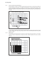
1
User Guide
English
Copyright © 2004, by Way Out Ware, Inc.. All rights reserved.
No part of this work may be reproduced or transmitted in any form or by any means, electronic or
mechanical, from or to any form of media, without the prior written permission of Way Out Ware, Inc..
Requests for permission to reproduce any part of this work should be addressed to : Way Out Ware,
Inc., attn: Copyright Adminstration, [email protected].
Table Of Contents
1
The TimewARP 2600 Manual . . . . . . . . . . . . . . . . . . . . . . . . . . . . . . . . . . . . . . . . . . . . . . . . . . . . . . . . . . . . . . . . . 3
1.1
1.2
1.3
1.4
2
The ARP 2600, 1970 - 1981 and Onward . . . . . . . . . . . . . . . . . . . . . . . . . . . . . . . . . . . . . . . . . . . . . . . . . . . . . . . . .
Foreword . . . . . . . . . . . . . . . . . . . . . . . . . . . . . . . . . . . . . . . . . . . . . . . . . . . . . . . . . . . . . . . . . . . . . . . . . . . . . . . . . .
How this Manual is Organized . . . . . . . . . . . . . . . . . . . . . . . . . . . . . . . . . . . . . . . . . . . . . . . . . . . . . . . . . . . . . . . . .
How To Use This Manual . . . . . . . . . . . . . . . . . . . . . . . . . . . . . . . . . . . . . . . . . . . . . . . . . . . . . . . . . . . . . . . . . . . . .
3
3
4
4
System Requirements, Installation, Configuration, Setup and Usage . . . . . . . . . . . . . . . . . . . . . . . 5
2.1 Digidesign Pro Tools . . . . . . . . . . . . . . . . . . . . . . . . . . . . . . . . . . . . . . . . . . . . . . . . . . . . . . . . . . . . . . . . . . . . . . . . . 5
2.2 MIDI Communication and Control . . . . . . . . . . . . . . . . . . . . . . . . . . . . . . . . . . . . . . . . . . . . . . . . . . . . . . . . . . . . . . .7
3
The Craft of Audio Synthesis . . . . . . . . . . . . . . . . . . . . . . . . . . . . . . . . . . . . . . . . . . . . . . . . . . . . . . . . . . . . . . . . . . 8
3.1
3.2
3.3
3.4
3.5
3.6
3.7
4
Modular Components of the TimewARP 2600 . . . . . . . . . . . . . . . . . . . . . . . . . . . . . . . . . . . . . . . . . . . . . . 29
4.1
4.2
4.3
4.4
4.5
4.6
4.7
4.8
4.9
4.10
4.11
4.12
4.13
4.14
5
6
Signals and Sounds. . . . . . . . . . . . . . . . . . . . . . . . . . . . . . . . . . . . . . . . . . . . . . . . . . . . . . . . . . . . . . . . . . . . . . . . . . 8
Attributes of Signals. . . . . . . . . . . . . . . . . . . . . . . . . . . . . . . . . . . . . . . . . . . . . . . . . . . . . . . . . . . . . . . . . . . . . . . . . . 9
Attributes of Auditory Events . . . . . . . . . . . . . . . . . . . . . . . . . . . . . . . . . . . . . . . . . . . . . . . . . . . . . . . . . . . . . . . . . . . 17
How Signals and Sounds Go Together... Sort of . . . . . . . . . . . . . . . . . . . . . . . . . . . . . . . . . . . . . . . . . . . . . . . . . . . 18
Modules and Methods for Generating Signals . . . . . . . . . . . . . . . . . . . . . . . . . . . . . . . . . . . . . . . . . . . . . . . . . . . . 21
Modules and Methods for Processing/Modifying Signals . . . . . . . . . . . . . . . . . . . . . . . . . . . . . . . . . . . . . . . . . . 23
Controlling One Module by Means of Another . . . . . . . . . . . . . . . . . . . . . . . . . . . . . . . . . . . . . . . . . . . . . . . . . . . 27
Top Row Control Panel Buttons and Indicators . . . . . . . . . . . . . . . . . . . . . . . . . . . . . . . . . . . . . . . . . . . . . . . . . . . 29
Preamp/Gain Control . . . . . . . . . . . . . . . . . . . . . . . . . . . . . . . . . . . . . . . . . . . . . . . . . . . . . . . . . . . . . . . . . . . . . . . 33
Voltage-Controlled Oscillators (VCO) . . . . . . . . . . . . . . . . . . . . . . . . . . . . . . . . . . . . . . . . . . . . . . . . . . . . . . . . . . . 34
Voltage Controlled Filter (VCF) . . . . . . . . . . . . . . . . . . . . . . . . . . . . . . . . . . . . . . . . . . . . . . . . . . . . . . . . . . . . . . . . . 36
Envelope Generators. . . . . . . . . . . . . . . . . . . . . . . . . . . . . . . . . . . . . . . . . . . . . . . . . . . . . . . . . . . . . . . . . . . . . . . . 37
Voltage Controlled Amplifier (VCA) . . . . . . . . . . . . . . . . . . . . . . . . . . . . . . . . . . . . . . . . . . . . . . . . . . . . . . . . . . . . . 39
Mix/Pan/Reverb Output Module . . . . . . . . . . . . . . . . . . . . . . . . . . . . . . . . . . . . . . . . . . . . . . . . . . . . . . . . . . . . . . 40
Envelope Follower . . . . . . . . . . . . . . . . . . . . . . . . . . . . . . . . . . . . . . . . . . . . . . . . . . . . . . . . . . . . . . . . . . . . . . . . . . . 41
Ring Modulator . . . . . . . . . . . . . . . . . . . . . . . . . . . . . . . . . . . . . . . . . . . . . . . . . . . . . . . . . . . . . . . . . . . . . . . . . . . . . 41
Noise Generator (NG) . . . . . . . . . . . . . . . . . . . . . . . . . . . . . . . . . . . . . . . . . . . . . . . . . . . . . . . . . . . . . . . . . . . . . . . 42
Voltage Processors (VP). . . . . . . . . . . . . . . . . . . . . . . . . . . . . . . . . . . . . . . . . . . . . . . . . . . . . . . . . . . . . . . . . . . . . . 43
The Sample & Hold Module (S/H) . . . . . . . . . . . . . . . . . . . . . . . . . . . . . . . . . . . . . . . . . . . . . . . . . . . . . . . . . . . . . 44
The Internal Clock /Electronic Switch . . . . . . . . . . . . . . . . . . . . . . . . . . . . . . . . . . . . . . . . . . . . . . . . . . . . . . . . . . . 44
The Virtual Keyboard. . . . . . . . . . . . . . . . . . . . . . . . . . . . . . . . . . . . . . . . . . . . . . . . . . . . . . . . . . . . . . . . . . . . . . . . 45
Patching the TimewARP 2600 . . . . . . . . . . . . . . . . . . . . . . . . . . . . . . . . . . . . . . . . . . . . . . . . . . . . . . . . . . . . . . . 46
Appendices . . . . . . . . . . . . . . . . . . . . . . . . . . . . . . . . . . . . . . . . . . . . . . . . . . . . . . . . . . . . . . . . . . . . . . . . . . . . . . . . . . 47
6.1 Table of Alternate Keyboard Tunings . . . . . . . . . . . . . . . . . . . . . . . . . . . . . . . . . . . . . . . . . . . . . . . . . . . . . . . . . . . 47
7
Contact . . . . . . . . . . . . . . . . . . . . . . . . . . . . . . . . . . . . . . . . . . . . . . . . . . . . . . . . . . . . . . . . . . . . . . . . . . . . . . . . . . . . . . . 49
TimewARP • User Guide
English
1.1
The TimewARP 2600 Manual
The ARP 2600, 1970 - 1981 and Onward
The ARP 2600 was the second product of ARP Instruments. It was released in 1970, and continued until the
manufacturer ceased operations in 1981.
Its design combined modularity (for studio flexibility, and for instructional use) and integration (for real-time
performance). Functionally, the ARP 2600 was completely modular: any signal output could be routed to any
signal input, with a patch cord. Operationally, the ARP 2600 was integrated, using internally-wired default signal
paths that made it possible to create a wide range of keyboard patches by simply opening up slide attenuators,
as though sitting in front of a mixing console.
The ARP 2600 earned an early reputation for stability, and for flexibility exceeding that of its competitor, the
Minimoog. Used 2600’s in good condition command premium prices on eBay today and businesses around the
country make a living reconditioning, rebuilding, and customizing 30-year-old units.
Among rock musicians, the ARP 2600 was used by Stevie Wonder, Pete Townsend, Joe Zawinul, Edgar Winter, Paul
Bley, Roger Powell, Jean-Michel Jarre, Mike Oldfield, Herbie Hancock, and many, many others.
Its modular design, and the popularity of its Owner’s Manual, made the ARP 2600 a widely used teaching
instrument in many schools and music conservatories around the country and internationally.
We are proud to bring you this software emulation of the 2600. Have fun with it, learn from it, but above all, make
noise with it.
1.2
Foreword
Unfasten the seat belts of your mind. The TimewARP 2600 will be an astonishing, exhilarating, and enlightening
experience.
Creating this manual has been an astonishing, exhilarating, and enlightening experience for me. How many are
ever given the chance to revisit an earlier life, an earlier project, a project like the ARP 2600 Manual, decades later,
and get it right? It’s time travel. I’m grateful to Way Out Ware for providing me that opportunity.
When, at Alan R. Pearlman’s invitation, I began work on the original 2600 manual in September of 1970, the 2600
itself barely existed. For the first two months, I was writing “blind”—without a machine in front of me. My first
hands-on experience with a synthesizer had been only six months earlier (it was a Putney VCS3).
I finished the text in March of 1971, Margaret Friend created the graphics, and the Owner’s Manual for the ARP
2600 began what turned out to be a surprisingly long career. In spite of the many defects that my inexperience
contributed—the gaps in coverage, and outright errors—it became quite popular. To this day, it still gets an
occasional respectable mention in the analog-synthesis community.
When Way Out Ware’s Jim Heintz called in early 2004 to tell me about the TimewARP 2600, a lot of time had
passed. Regarding software synthesizers, I had grown weary and cynical. Analog-modeling software had been
a decade-long disappointment; some products did interesting things but not the things that real analog modules
do. Jim, however, had already encountered, thought about, and solved these problems. He owned a real 2600.
He really aimed at getting it right and would not be satisfied with anything less. It was a pleasure, finally, to accept
his invitation to do an Owner’s Manual.
It’s now clear that Way Out Ware has set a new standard for software-based audio synthesis. The behavior of the
TimewARP 2600 software—both module-by-module and integrated into patches—is effectively indistinguishable
from that of the analog hardware that it emulates.
Soaring and swooping through the free air of analog synthesis—a world of nothing but sliders and cords and
continuously evolving patch configuration—was a capstone course at the Boston School of Electronic Music in
the 1970’s. That is the world that the TimewARP 2600, for a new generation of musicians in a new millennium
(that means you), provides access to: it is the first—and I believe only—software synthesizer to support real-time
performance by sliders and patchcords alone.
So here it is: your new Owner’s Manual, for the new TimewARP 2600.
Unfasten the seat belts of your mind. How else can you hope to experience time travel? How else can you enjoy
free flight?
Jim Michmerhuizen
Jim Michmerhuizen is the author of the original ARP 2600 Manual and Founder and Director of the Boston
School of Electronic Music.
3
English
1
1.3
How this Manual is Organized
This is not a textbook; it’s a survival manual.
Chapter 2 is about installing and configuring the software so you can get up and running.
Chapter 3 is a brief introduction to the vocabulary and methods of classical analog synthesis, so that we can
understand each other throughout the rest of the book.
Chapter 4 is a module-by-module reference, including the digital extensions made possible by the fact that the
TimewARP 2600 is software—a piece of computer behavior—rather than a collection of electronic hardware.
Chapter 5 is not in this book, but is a collection of patches, with accompanying documentation, located in a separate
document file called Patchman.pdf found on the distribution CD (or as a download from www.wayoutware.com).
The patches and commentary are keyed to the numbered chapters, sections, and subsections of this manual.
Some of the patches form a tutorial sequence, and some illustrate vocabulary lessons and concepts.
1.4
How To Use This Manual
You’ll probably need to do a quick run through of Chapter 2 as you install the TimewARP 2600 and learn some of
the basic setup operations. After that, you can pretty much mix and match, according to your experience.
If you’re new to audio synthesis, you’ll want to walk through the tutorial patch sequence in Patchman.pdf, referring
back to Chapter 3 for concepts and Chapter 4 for detailed module specifications while you explore, and learn to
control, the vast range and patch repertoire of the TimewARP 2600 software synthesizer.
If you already have some experience with audio synthesis, you might go directly to Chapter 4 for the detailed
module-by-module specifications of the TimewARP 2600. If you know and love the original ARP 2600 itself, take
particular note of section 4.1, where we describe what you can do with the TimewARP 2600 that you could not do
with its analog ancestor. These digital extensions include patch load/save, additional VCO sine-wave outputs,
dual-channel signal input, automatic Y-connections at all signal outputs, sixteen keyboard micro-tuning options,
MIDI Beat Clock synchronization, and MIDI controller mapping (with subranges) for all the panel sliders.
4
TimewARP • User Guide
System Requirements, Installation, Configuration, Setup and Usage
In this chapter you will find all of the platform-dependent information you need in order to install and operate your
TimewARP 2600 software synthesizer.
The TimewARP 2600 provides an extended set of digitally-based features that no hardware-based analog
synthesizer can offer. We describe the most important of these in section 2.2.
2.1
Digidesign Pro Tools
This release of the TimewARP 2600 is an RTAS plug-in and runs only under Digidesign Pro Tools 6.1 and later
versions, on either Apple OS X or Windows XP. On either of these platforms, the requirements for the TimewARP
2600 are essentially those of Pro Tools itself.
2.1.1
System Requirements
These are the same as Pro Tools itself, including enough memory to satisfy the practical needs of the TimewARP
2600 software.
2.1.1.1
Disk Space and RAM
The executable file occupies 6.1MB on disc, and the RAM requirements when running are the same as the Pro
Tools minimums.
2.1.1.2
System Clock
The TimewARP 2600 performs all signal generation and processing in real time. In complex polyphonic patches,
this may put a considerable load on your CPU. You may have difficulty with a clock speed less than 800MHz;
higher clock rates will increase the number of polyphonic voices you can use, and the complexity of the patches
available.
2.1.2
Installation
Installation on either platform is accomplished by very simple standardized installation sequences. You must, of
course, have a current installation of Pro Tools on your target computer.
2.1.2.1
Mac OS X
Insert the distribution CD or download the .dmg installer file from www.wayoutware.com. Double-click the .dmg
installer to initiate installation.
If you agreed to the license, a TimewARP 2600 installer icon appears. Double-click it to initiate the installation
process.
When finished, start Pro Tools and proceed to 2.1.3.1.
2.1.2.2
Windows XP
Insert the distribution CD or download the installer file from www.wayoutware.com. Run the .exe installer file.
If you agreed to the license, follow the installer instructions.
When finished, start Pro Tools and proceed to 2.1.3.1.
2.1.3
Setups
2.1.3.1
Real-time Instrument for Performance and Recording
The TimewARP 2600 can transform your computer into a real-time instrument for live performance or recording.
To set this up, create an audio track in Pro Tools. Select either mono or stereo in the track-creation window; this
will determine, in turn, the channel options offered by the TimewARP 2600 for this track.
In the mix window display for this track, at the track-inserts block up at the top, click on the first insert selector.
Choose the TimewARP 2600 plug-in from the appropriate menu.
Now create another track, but in the track creation dialog, choose MIDI track instead of audio track, and route the
track output to the TimewARP 2600.
As input for the new track, select your MIDI keyboard device, and enable the track for recording. Pro Tools will
route all incoming MIDI events from your MIDI keyboard device to the TimewARP 2600 plug-in.
If your MIDI keyboard has any additional MIDI control devices (sliders, knobs, buttons, etc.), you can assign these
to any TimewARP 2600 sliders, knobs and switches that you choose. For details, see section 2.2.
5
English
2
2.1.3.2
Processing Audio Signals
The TimewARP 2600 can be used to process audio signals in a similar manner to a reverb or other effects plugin.
To set this up, create an audio track or select a track already recorded in Pro Tools. (If this is a new track, select
either mono or stereo in the track-creation window; this will determine, in turn, the channel options offered by the
TimewARP 2600 for this track.)
In the mix window display for this track, at the track-inserts block up at the top, click on the first available insert
selector. Choose the TimewARP 2600 plug-in from the appropriate menu.
If the current track is mono, the TimewARP 2600 for this track will be configured for one channel of input, and you can
select between mono and stereo output. If the current track is stereo, the TimewARP 2600 insert will automatically
be configured for stereo throughout. Confirm this, when the synthesizer panel comes up, by observing that the
preamp module in the upper left corner has two channel outputs rather than just one.
If you are processing an existing track, press play on the transport control to hear the audio being processed by
the TimewARP 2600 in real time. You need to select an appropriate TimewARP 2600 patch (such as those in the
Voice or Guitar Effects categories in the Factory group) to successfully process audio this way.
If you are processing a live track, enable the track’s record mode, and then audio from your input will be fed
through the TimewARP 2600. You need to select an appropriate TimewARP 2600 patch (such as those in the Voice
or Guitar Effects categories in the Factory group) to successfully process audio this way.
2.1.3.3
MIDI Tracks
Running as a track plug-in, the TimewARP 2600 can process prerecorded MIDI tracks.
To do this, set up two tracks just as you did above in section 2.1.3.1: an audio track that is running the TimewARP
2600 as a track insert, and a MIDI track whose output is routed to the TimewARP 2600.
When you play this track (use the Pro Tools transport window to play, rewind, pause the MIDI sequence, etc.), the
MIDI events stored in the track sequence will be routed to the TimewARP 2600. MIDI note-events will become
key depressions at the virtual keyboard; MIDI pitch-bend will turn the virtual keyboard pitch-bend knob; and
MIDI controllers that are mapped to TimewARP 2600 sliders, knobs or switches (see section 2.2) will move those
controls.
2.1.4
Selecting Patches
The TimewARP 2600 gives you a three-level hierarchy for storing and organizing your patches. All Patches are
sorted into various Categories, which are in turn sorted into major Groups. Each of the three patch selection
buttons generates a drop-down list associated with one layer in this hierarchy.
Groups, Categories, and Patches can also be selected by keyboard shortcuts. The up/down arrow keys on the
computer keyboard select Patches, the left/right arrow keys move between Categories, and using the control key
with the left/right arrow keys moves between Groups.
2.1.5
Making Patch Connections
Use the mouse to connect any output to any input jack. Position the cursor at any signal output, click and hold
down the mouse button, and drag the patch cord to any signal input. To remove a patch cord, drag either end
away from its signal jack.
The TimewARP 2600 will not connect two outputs or two inputs together. If you drag from one jack to another but
no patch cord appears, it may be that both jacks are inputs or both are outputs.
The TimewARP 2600 will allow Y-connections, distributing a single output signal to multiple destinations by holding
the control key down while clicking an output that already has a cable connected to it. A second cable will appear
attached to the cursor, which can then be plugged into another input.
2.1.6
Using the Sliders and Knobs
To adjust a slider or knob, drag it with the mouse. For increased resolution, hold down the command (Apple) or
control (Windows) key during the drag operation.
If you pause for a moment over a slider, a display will pop up with the numerical value and name of the parameter
it controls.
If you have MIDI controller hardware, you can easily connect it to the sliders, knobs or switches; see section
2.2.2.
6
2.1.7
Using the Virtual Keyboard Display
The graphic TimewARP 2600 keyboard display responds directly to mouse events; click on any key to create a MIDI
“keydown” signal. This is useful when you are creating and tuning a new patch, if you don’t have a hardware
MIDI keyboard handy.
The virtual keyboard also displays—as key depressions—incoming MIDI note-events. Use this to monitor your
external MIDI keyboard connection and activity.
2.1.8
Polyphonic Operation
The TimewARP 2600 can respond to as many as eight simultaneous keydown events. Use the Voices dropdown
(see section 4.1.1.2) to set the number of voices.
2.1.9
Saving and Loading Patches
You may save patches using the Save or Save As buttons or load patches with the Patch Manager (see section 4.1
below). There is no limit to the number of patches you can create and save. To enable the Save button, the Lock
button (padlock icon) must be in the unlocked mode.
You may wish to create a bank of “template” patches, generic versions of often-used configurations.
The TimewARP 2600 responds to MIDI bank-select and patch-select commands.
2.2
MIDI Communication and Control
2.2.1
Slider, Knob and Switch Control
You may control any slider, knob or switch on the TimewARP 2600 plug-in with any MIDI controller. If you have a
hardware control surface, or if your MIDI keyboard has slider or knob control devices, you can use them to control
any combination of sliders, knobs or switches in a patch.
Any connections you set up are global to the TimewARP 2600—you can store them independently of any specific
patch (see section 4.1.2.1 below).
To connect a slider, knob, or switch to an external MIDI controller, hold down the control (Mac) or shift (Windows)
key and click on the slider, knob or switch image. The responding dialog box offers you both global and patchspecific connections.
2.2.1.1
Global MIDI Map Settings
Select the controller number, either by directly typing it in, or by moving the physical control on the MIDI device you
intend to use.
Set the response curve, polarity, and range. The response curve may be linear, or exponential, or logarithmic. The
polarity is either direct or inverted. To set the Control Range, drag either end of the bar inward. Whenever the bar
covers less than the entire controller range, you may also drag it to the right or left, to adjust the range offset.
You may, if you wish, assign the same external control to several TimewARP 2600 sliders or knobs, and set a
different curve, polarity, and range for each one. In this way, you can create patches and configurations of the
TimewARP 2600 that are specifically adapted for expressive performance either live or in the studio.
2.2.1.2
Patch-Specific Settings
Besides globally assigning a slider, knob or switch to a MIDI controller, you may also assign the slider or knob to
be controlled by the velocity and/or aftertouch parameters of incoming keyboard events. (These assignments are
not global; they are stored with individual patches.)
In real time, these controller values are summed with the current global control values to determine the real-time
value of the slider. So, by careful tuning beforehand, you can have both keyboard expression and hardware
knob/slider control at the same time.
2.2.2
MIDI Patch Selection
In each group of patches, the first 128 are available to standard incoming MIDI patch-selection commands.
Patch categories don’t affect this numbering. For example, if the first category in a group has 127 patches, then
the second category will have just one patch available for MIDI patch selection.
Groups themselves can be selected with MIDI bank-select commands.
7
English
TimewARP • User Guide
3
The Craft of Audio Synthesis
This chapter is about the facts—physical, mathematical, and auditory—that make the TimewARP 2600, and the hardware
that it emulates, possible. We have to spend a few minutes here distinguishing between physical signals, and the sounds
that people hear in the presence of certain kinds of signals.
This is important because synthesizer equipment can only deal with signals—physical commotion of one sort and another.
When you are fiddling with synthesizer equipment, you are generating and modifying signals for the sake of the interesting
(we hope) sounds you hear when those signals reach your eardrums.
3.1
Signals and Sounds
A signal is something happening: a waving flashlight, or ambulance siren, referee flag dropping, winking at a friend. Tiny
disturbances of the air around us are signals for our ears; we hear them as noise, or singing, or sirens, shrieks, growls,
whatever.
The signal is the physical disturbance in the air, the movement of the eardrum. The sound is your perception of the signal:
“Hello!”
3.1.1
Analog and Digital Representations of Signals
The signals we are concerned with in sound synthesis are audio signals: more or less regular variations in air pressure, at
our eardrums, repeating at rates of between 20 and 20,000 times in one second.
Such signals are straightforward physical processes which can be recorded and reproduced. One way to do that is to look
at the pattern of air-pressure variation, and model it in some other medium. During the past century this has been done
with grooves in a phonograph record, magnetic fields along a length of tape or wire, and other media. The usual scenario
is: with one or more microphones, generate an electronic model of the vibrating air, then use the electronic signal to drive
a magnetic recording head, or amplifier, or LP recording lathe. Throughout such processing, the signals we deal with are
directly analogous to each other; except for the change in medium from air to voltage to magnetic field strength or stylus
position, the signals are identical. Graphed or charted, they even look the same. This is analog recording.
8
TimewARP • User Guide
Since the TimewARP 2600 is not constructed of electronic circuits, concepts such as “voltage” don’t apply here. The TimewARP
2600 is software, a complex piece of computer behavior. The signal medium for the original ARP 2600 was electrical
pressure, measured in volts. The signal medium for the TimewARP 2600 is simply number sequences. We use those
numbers the way the original machine used electrical pressure; where the original Owner’s Manual used the word “voltage”
we will just say “signal” or “signal level,” and in the module specifications we will refer to “virtual Volts” or “vV.”
3.2
Attributes of Signals
The simplest possible signal is a sine wave. It’s like the back-and-forth motion of a point on a circle as the circle rotates. A
lot of the mathematics of sine waves is based on that rotating-circle idea; you don’t have to get involved in that unless you’re
curious about it, but it’s helpful to train your imagination by picturing the basic sine-wave graph as a slightly stretched coil
spring like a “slinky.”
The motion of a pendulum, or of a tuning fork, swinging back and forth as they slowly come to rest, is a decaying sine
wave.
A sine wave signal has exactly three attributes: its frequency, its amplitude, and its phase. It has no other characteristics at
all. (The decaying swing of the pendulum or the tuning fork does have one other attribute: the amount of energy/amplitude
that it loses on each swing. It’s not a “pure” sine wave.)
3.2.1
Fundamental Attributes
Picture a point on that rotating circle, leaving a trail behind as it rotates, like an airplane propeller. Picture the trail, stretched
out behind like a coil spring, and ask yourself:
3.2.1.1
Amplitude: what’s the diameter of this imaginary circle?
3.2.1.2
Frequency: how fast is it rotating?
3.2.1.3
Phase: when does it start a new cycle?
9
English
Another way to record such a signal is, with high-speed digital circuits, to measure the underlying medium many times each
second, and store the measured numbers. This is digital recording.
3.2.2
Complex Attributes
Most of the activity that reaches our ears every day is far more complex than just a sine wave. Banging on a
garbage can creates a much more complicated sort of vibration than tapping a tuning fork.
But any kind of motion that isn’t a sine wave can still be analyzed as a collection of sine waves. This is called
Fourier analysis, after the man who discovered that it was possible, and proved—mathematically—that it always
worked.
This goes both ways: any complex signal can also be constructed from a collection of sine waves with the
appropriate attributes: amplitude, frequency, and phase relationships.
In fact, any kind of motion—any repeating pattern of the sort that we are interested in here as “sound waves”—
can be examined and analyzed under two different headings:
10
3.2.2.1
Waveshape, and Time-Domain Attributes
Any repeating motion can be diagrammed in a graph where the horizontal axis is a period of time and the vertical
one is the motion itself, back and forth. This is the time-domain view of a signal:
11
English
TimewARP • User Guide
3.2.2.2
Spectrum, and Frequency-Domain Attributes
Instead of looking at a signal as something in motion through a period of time, we can look at the collection of
sine-wave components of the signal. In such graphs, the horizontal axis is a frequency range (instead of a time
period), and we indicate each spectrum component with a single vertical line in the graph. The height of the line
indicates the strength of the component at that frequency. This is the frequency-domain, or spectral-domain, view
of a signal.
It is the distribution and relative strength of spectral components that we experience as the tone-color of a sound
or sounds. “Bright,” “dull,” “sharp,” “tinny,” “heavy,” and so on—these are all descriptive words for the spectral
attributes of sounds.
3.2.2.2.1
Harmonic Series
The spectral view of any periodic signal has components at simple multiples of the signal frequency. For example,
suppose we examine a sawtooth wave at a frequency of 110Hz. It will have components at 110, 220, 330, 440,
and so on.
12
TimewARP • User Guide
English
A simple number sequence like this is called a harmonic series. It is interesting to think about musically; the
smaller numbers in the series all form simple musical intervals: octaves, fifths, fourths, and thirds.
Most musical instruments generate harmonic spectra. Some have more, some have fewer harmonics, and there
are wide spectral variations even within a single instrument depending on how it is played. In general, whatever
the actual spectral components are, they will always form a harmonic series.
In audio synthesis, you will use oscillators to generate pitched tones that have a harmonic spectrum.
13
3.2.2.2.2
Inharmonic Series
Inharmonic, in this context, means “not forming a harmonic series.” Some waveforms do not repeat themselves
at a regular interval; the spectra of such waves will have components at strange non-integral frequency ratios, or
they may have shifting spectral components that die out and reappear. Some percussion instruments, such as
kettledrums, or bells, have inharmonic spectral components.
In audio synthesis, you can use various modulation techniques—such as AM and FM—to generate inharmonic
spectra.
14
3.2.3
Attributes of Random Signals
A completely random signal—noise—actually has a continuous spectrum: it does not consist of isolated sine
waves in a harmonic series, nor even in an inharmonic series. A noise spectrum is a continuum of frequency
components; in order to describe it, we have to talk about how much energy is in each band in this continuum.
One kind of noise may have high-frequency energy, while another has low-frequency energy.
In audio synthesis, noise is an extraordinarily useful signal. Filters can be used to shape a noise spectrum into
almost anything—even pitched sounds.
15
English
TimewARP • User Guide
3.2.3.1
Spectral Balance (Color)
The physical processes (such as molecular motion or random popping of electrons from one atom to another)
that we typically depend on for random electronic noise have a frequency distribution of equal probability at
any frequency, or through any frequency interval. Curiously enough, this produces noise signals that, for audio
purposes, don’t sound properly balanced across our range of hearing. They sound too bright.
16
TimewARP • User Guide
Attributes of Auditory Events
Of all the thousands of sounds you hear in a single day, only some have a definite beginning or ending point.
Many just come and go without a clear start/stop. Those that do have a reasonably clear start/stop we will call
auditory events. The other sounds, the less clearly defined ones, we can call auditory textures or backgrounds or
even structures.
Think how some sounds are more complicated than others. The hum of a refrigerator is sort of simple, the hum of
a tuning fork is (as we heard above) really simple. A single bass note from a piano is quite complicated, the way it
keeps changing and evolving as it dies away. Human speech is a very complicated kind of sound, even when it’s
your native tongue (when it’s a language you don’t understand, it sounds even more complicated).
There are many, many more kinds of sounds to hear than you or I have words to describe them with. Here are just
a couple of the most general distinctions people make about different kinds of sounds:
17
English
3.3
3.3.1
Steady-State Attributes:
Some sounds, once they get started, remain pretty constant. They don’t change much while they continue, and
when they stop, they just stop. We say such sounds reach a steady state, in which we can pick out a definite
Pitch, Loudness, and Tone Color. Notes from organ pipes—or from electronic drawbar organs—are steady-state
sounds.
3.3.2
Time-Varying Attributes (i.e. “Envelopes”):
Some sounds have a pretty clear start and end, but while they’re happening they change. Think of a bird song,
or ordinary human speech.
Such sounds can sometimes be analyzed as more or less rapidly changing in one or more of those fundamental
auditory attributes: pitch, loudness, or tone-color. Think, for example, of how the sound of a plucked guitar string
evolves from the moment you pick it to the moment you can’t hear it anymore. It starts out loud and fades away;
and it starts out “bright”—with lots of harmonics—and is slowly “muffled” as it fades out.
One way to conveniently diagram what happens in such events is to chart each changing attribute separately, in
its own time-domain graph.
Such a graph is often referred to as an envelope. Over the years, some standard vocabulary has developed for
talking about envelopes: Attack (for the first part of an event), Decay (for some later parts), and Release (for the last
part, when the event is coming to an end).
3.4
How Signals and Sounds Go Together... Sort of
Signal activities, being entirely physical kinds of things, are easily nameable, measurable, catalog-able, and
countable. Sounds, as we pointed out above, are not quite so easily domesticated. The music and other sounds
that we listen to correlate in several well-established ways with the signals around us, but the correspondence is
not simple. There are always surprises.
3.4.1
Signal Frequency and Audible Pitch
This is probably the best-established and most reliable correspondence. It dates all the way back to Pythagoras,
the Greek philosopher who 2500 years ago worked out that halving the length of a vibrating string made the pitch
rise by one octave.
18
3.4.1.1
How Adding Pitches Means Multiplying Frequencies
The range of audio frequencies—of human hearing, in other words—is conventionally stated to be 20Hz to 20KHz.
And when you think linearly, it sounds tragic to learn of someone, say, who can only hear up to 10kHz. But in the
realm of human pitch perception, such a person has kept 90% of his hearing range: from 10kHz to 20kHz is just
one octave out of the 10 we hear.
This is a really important fact in audio synthesis; you will encounter it over and over again, in every patch you
create. It governs much of the arithmetic of generating and controlling spectral distributions and patches:
• Equal pitch intervals require exponentially increasing frequency increments;
• Equal frequency increments make a harmonic series. In a harmonic series, as we go up the series we get
smaller and smaller pitch intervals.
3.4.2
Signal Amplitude and Audible Volume
This is a very dicey relationship. It is true that, for any given signal, increasing its amplitude will increase the
volume of the associated sound. But a lot of other signal characteristics have a greater impact on our perception
of volume than amplitude does.
For example, the difference between talking and shouting at someone is far more a matter of pitch and spectrum—
tone-color—than of mere amplitude. When I yell, I “raise my voice”; that is, I raise the pitch of my voice, and I put
more energy into it, which generates more harmonics, which is a matter of spectral content, not amplitude. Stage
actors have to learn to overcome this tendency; in order to be heard onstage without shouting, they have to learn
to increase their speaking amplitude without yelling.
If you examine—visually—the recorded signal from a pipe organ, or even an orchestra, you may be surprised
to find the apparent amplitude of the softer signals almost equal to that of the loudest. This has to do with the
spectral distribution of the sound. Of two different signals of approximately equal amplitude, the one with the
broadest spectral distribution—the most harmonic content—will sound louder.
19
English
TimewARP • User Guide
3.4.2.1
How Adding Volumes Means Multiplying Amplitudes
Nonetheless, for a given signal and its spectrum, it is always true that a bare increase in amplitude will be heard
as an increase in loudness. But how much of an increase?
It turns out that, just as with frequency and pitch, the relationship here is exponential. A century of research has
established that equal steps in loudness are represented by multiplicative ratios in signal amplitude.
In other words, if you double the amplitude of a signal, you will hear an increase in loudness. But then to get
another increase equal to the first one, you have to double the amplitude again.
3.4.3
Signal Spectrum and Audible Tone-Color
This is a quite solid relationship. In fact, the word “spectrum” has achieved a meaning in both worlds: depending
on the context, it can refer to a measurable attribute of physical signals, or a character of perceived sounds.
Any change you hear in the character of a sound—in its tone-color or “spectrum”—must have an associated
variation in the character of the physical signal that is arriving at your eardrums. Tone change = waveform
change.
The reverse is not quite so certain. It’s fairly easy to find waveform changes that listeners can’t hear. For example,
we humans simply aren’t sensitive to phase relationships within a complex spectrum. But, in the time domain, two
identical spectra with shifted phase relationships among their components can look unrecognizably different.
3.4.4
Signal Envelopes and Audible Event-Contours
One of the most fascinating areas of audio synthesis is listening for the envelopes of time-varying events. Here
there are all sorts of mysteries, in which signal attributes get regularly “misperceived”: frequency variations get
heard as volume, spectral evolutions are heard as pitch, and amplitude envelopes generate an elusive spectral
twitter.
20
TimewARP • User Guide
Modules and Methods for Generating Signals
How can you get access to the signals and processes we’ve just described, so that you can play with them on
your own?
Throughout the past century people have been noodling around with electronic ways of generating audio signals.
In particular, beginning in the 1960’s, people such as Bob Moog, Don Buchla, and Alan R. Pearlman began to settle
on some ideas that have become almost standard for audio synthesis: independent, modular functions for signal
generation and signal processing, capable of being controlled not only by hand but also by signals of the same
kind as they generate.
This was the idea of voltage-controlled operation, and it was completely revolutionary. Using independent, modular
functions made it possible to change one attribute of a signal without necessarily affecting any other attribute; so
the craft of synthesis became the craft of constructing, and tuning, integrated configurations of modules.
The cables that connected modules were called patchcords, and so connecting modules together came to referred
to as patching them, and so, finally, any working configuration came to be called a patch.
Let’s take a look at some modules that generate signals.
3.5.1
Oscillators
A device that repeats the same motion over and over is an oscillator. In audio synthesis, oscillators typically
produce very simple geometrical-pattern signals such as sine, triangle, pulse, and sawtooth waves, named simply
for what their time-domain graphs look like.
In an analog synthesizer, the underlying medium in motion is usually electrical pressure, or voltage. In a digital
synthesizer, the signal is actually generated as a sequence of calculated numbers. (Conventionally, these are
generated at the standard sampling rate for music CDs, 44.1KHz.) This does not become motion until, at the output
of the synthesizer, the number stream is converted to variations in voltage, and then amplified, and then used to
drive a loudspeaker. (A loudspeaker is a motor that moves back and forth instead of around and around.)
Because oscillator-generated signals are periodic, their spectral components always form a harmonic series.
21
English
3.5
3.5.2
Noise Generators
A device that jiggles at random without ever repeating itself is a noise generator. Waterfalls, steam, wind, fans,
and such things are all noise generators.
The spectrum of a noise signal is a statistical distribution of frequency components. (This is the opposite of a sine
wave, which is exactly one frequency.) A noise spectrum that is perfectly balanced throughout the musical range
is called pink noise. Pink noise is very useful in listening tests of loudspeakers, because a trained human listener
can hear even tiny differences between two different noise spectra.
Filtering and equalization can shape a noise spectrum into almost any sound.
3.5.3
Envelope Generators
A device whose output is intended to control some time-varying attribute of an event is called an envelope
generator. These are sometimes referred to as transient generators, to call attention to the fact that their output
is not constant but transient.
An envelope generator produces an output signal only “on demand.” The demand is made by means of timing
signals called gates, and triggers.
envelope generators are controlled by gate
and trigger signals...
gate
trigger
ADSR
envelope
AR
envelope
3.5.4
Sample & Hold Processors
The idea of “sampling” a signal does not directly relate to any particular characteristic of audio events; instead, it
is an idea from electronics that has turned out to be useful for creating patterned control signals.
22
3.6
Modules and Methods for Processing/Modifying Signals
3.6.1
Inverters
A signal inverter works exactly like a seesaw. When the input goes high, the output goes low, and vice versa.
An analog inverter would output negative voltages on positive input; a digital inverter simply multiplies its input
number-stream by (-1).
3.6.2
Signal Mixing
A signal mixer adds two or more signals together and outputs the result of the addition. This is a more complex
signal, usually, than any of the inputs. But not necessarily; if signal B, for example, is the exact inversion of signal
A, then mixing the two will produce a signal of exactly zero.
3.6.3
Attenuators/Amplifiers
An attenuator cuts the strength of a signal passing through. Digitally, this is accomplished by multiplying the
input by some value ranging from 0.0 (which passes no signal) to 1.0 (which passes the signal at its full input
amplitude).
An amplifier may increase the amplitude of a signal. But not necessarily; it is usual for a voltage-controlled
amplifier to have a maximum gain factor of 1.0. In fact, the purpose of VCA’s is actually to “chop” the signals
passing through them. It would make more sense to think of them as “voltage controlled attenuators.”
23
English
TimewARP • User Guide
3.6.3.1
Gain Factor
To describe the behavior of an amplifier or attenuator, we may use the expression “gain factor” to mean the ratio
of output signal amplitude to input amplitude.
3.6.4
Filters
A filter is a device that works better at some frequencies than at others. (The inverters, mixers, and attenuators we
have been describing work the same at all frequencies, so they are not filters.)
Because of this frequency-dependent characteristic of filters, they change the shape of any complex waveform
passing through. And so it will be important for you to get to know what filters do to signals in both the time
domain and in the frequency domain.
3.6.4.1
Low-Pass Filters
Any device or mechanism that passes along slower motions better than faster ones can act as a lowpass filter.
Picture yourself stirring a cup of tea with one of those little wooden paddles they hand out in the coffee shops. Stir
it back and forth, fast. Now slow down. Now imagine the tea has turned to syrup. You can still stir it slowly, but if
you try to go fast the stick will simply not move.
That’s a lowpass filter. You can see the effect of this on a signal quite easily.
For audio signals, you will usually be more interested in the frequency-domain effects of filtering. For subaudio
signals, it is usually the time-domain effects—changes in waveshape—that we care about. In the time domain, a
low-pass filter rounds off any sharp transitions in the signal. A good example of this is the lag processor described
in section 3.6.4.5 below.
In the frequency domain, it weakens spectral components that are higher than the filter cutoff frequency—the
frequency at which the filter begins to have an effect on the signal.
24
TimewARP • User Guide
High-Pass Filters
Any device or mechanism that passes along faster motions better than slower ones is a high-pass filter.
Take the drinking straw from your water glass. Seal the end of it with your thumb and dip it back into the water.
Notice that you can pump it up and down in the glass, fast or slow, but the water never leaks into the straw as
long as you hold your thumb over the end. Think of the up and down motion of the water at the bottom end of
the straw as “the signal.”
Now start letting a little air leak into the straw as you move it up and down. The water level at the bottom end of
the straw no longer stays down when the straw “signal” goes down—it starts to come up again. And then when
you draw the straw back up, the water leaks back down more or less rapidly depending on the position of your
thumb at the top of the straw.
This is a high-pass filter. In the time domain, it constantly “leaks” its output signal level back to zero, at a rate
related to the cutoff frequency and slope. In the frequency domain, it passes all spectral components higher than
the cutoff frequency, and attenuates those below the cutoff frequency by an amount proportional to the cutoff
slope.
3.6.4.3
Cutoff Slope
This is the rate at which a filter attenuates spectral components, as a function of their frequency. It is usually a
multiple of 6dB/octave.
3.6.4.4
Feedback and Resonance
It is usually possible, with any signal-processing device or system of devices, to mix some of its output signal back
into the input signal. This may be intentional, or it can happen by accident; everybody who has ever worked with
a PA system has experienced the terrible screech of a system “in feedback.”
In filter modules for audio synthesis, it is common to provide controllable feedback. With just a little, the filter
response begins to peak around its cutoff frequency; as the feedback level increases, the peak gets stronger.
Eventually—just as happens with a PA system—the filter falls into oscillation. Regardless of the input signal, it
“screams” a sine-wave at its cutoff frequency. In this state it is no longer behaving as a filter at all; it has become
an oscillator.
Systems in feedback have been very well studied in physics. Their behavior can be described mathematically.
Whereas feedback in a PA system can be unpredictable and uncontrollable, feedback in a filter module for audio
synthesis can be—and is—a controllable and useful feature.
3.6.4.5
Lag Processors
A lag processor is a low-pass filter intended specifically for processing sub-audio signals. It introduces a “lag” in
the output signal wherever the input shows a sharp change in value. How much of a lag depends on the “cutoff
frequency” of the processor.
25
English
3.6.4.2
3.6.5
Modulation Methods
The simplest possible signal, we said above, has exactly three attributes and no more: frequency, amplitude,
and phase. If, starting from a steady-state signal, we systematically modify any of these characteristics, we
are said to be modulating the signal. And so, based on these three signal attributes, there are three possible
forms of modulation: Amplitude Modulation (AM), Frequency Modulation (FM), and Phase Modulation (PM). The
first two are more commonly used in audio synthesis than the third; we won’t say anything here about phase
modulation.
Using AM and FM methods, it is possible to generate waveforms and spectra that are far more complicated—and
interesting to the ear—than anything that can be produced by merely mixing and filtering signals. Mainly that is
because of sidebands.
3.6.5.1
Sidebands and Sideband Spectra
What happens to the spectrum of a sine wave when we modulate its amplitude? What happens when we
modulate its frequency?
Clearly, since the signal that results from AM or FM methods is no longer a plain vanilla sine wave, then, in the
frequency domain, it must have some additional components. These additional components are called sidebands.
They have been studied for at least a century, and are pretty well understood physically and mathematically.
Audio synthesis is probably the only application of AM or FM modulation where we are interested in sidebands
for their own sake, as something to listen to directly; in the past, this kind of thing was only interesting to radio
engineers, radar, sonar, television broadcast engineering. In those disciplines, modulation sidebands are products
of broadcasting methods, in the electromagnetic spectrum. Because of that historical background, some of the
conventional language for talking about modulation processes is a little weird: the signal being modulated is
often referred to as the carrier signal, and the signal that provides the modulation pattern is called the program.
(Guess why?)
Any form of modulation generates, for each component of the original signal, at least one lower sideband—
at a frequency equal to the component minus the modulating frequency—and at least one upper sideband,
at a frequency equal to the component plus the modulating frequency. If the carrier—the original signal—is
itself complex, with multiple spectral components, then each of its components will produce its own sidebands
independently of all the others. Likewise, if the modulating signal—the program—is complex, the arithmetic
applies separately to each of its components.
26
So, just for example, if you modulate a 10-component carrier signal with a 10-component program signal, the
signal resulting from the modulation will have not less than 100 spectral components. This can get very messy;
the most useful thing you can do with such a signal, before you do anything else, is filter it to get rid of some of
the fuzz.
3.6.5.2
Amplitude Modulation
Suppose we modulate the amplitude of a 1000Hz sine wave with a 5Hz sine wave. The result is indistinguishable
from what we would get if we mixed three sine waves, at 995Hz, 1kHz, and 1005Hz. They are the same signal.
The 995Hz component of the output is the lower sideband resulting from the modulation, and the 1005Hz
component is the upper sideband.
3.6.5.2.1
Ring Modulation
While a VCA responds only to a positive-going signal at its amplitude-control input, a ring modulator responds
to both positive and negative levels at both of its inputs. Its output is simply the product, arithmetically, of the two
inputs. If you are new to audio synthesis, draw a couple of signal graphs—it doesn’t matter what they are—on the
same timebase and vertical scale, and use a pocket calculator to work out the result of multiplying the two signals
together. That’s what a ring modulator does. (The expression “ring modulator” describes the appearance of the
analogue circuit design that’s required for the multiplication.)
In the frequency domain, the difference between this and ordinary AM is only that the carrier signal components
are suppressed. Once again, if you work out the arithmetic, a single-frequency carrier, modulated by a singlecomponent program, generates a three-component AM spectrum but only a two-component ring-modulation
spectrum.
What’s useful about this? Well, since the carrier is almost always periodic (it comes from an oscillator, right?), it
has a harmonic spectrum. Suppressing this spectrum lets you hear just the sidebands, which can be completely
inharmonic if you’re careful about the ratio of the two input signal frequencies.
3.6.5.2.2
Frequency Shifting
It’s theoretically possible not only to suppress the original carrier, as in ring modulation, but to isolate the lower
and upper sidebands and make them available separately. The arithmetic here is fascinating, because the end
result (for once) is in one-to-one correspondence with the input: for each component of the program signal, there
is a component in the output at C-p (or at C+p). In other words, the final spectrum has only as many components
as the original program did. This is called frequency shifting. Picture the entire program signal spectrum shifted
up or down by some fixed frequency.
The important thing to remember about this is that it’s not pitch shifting—which would have to be accomplished
by frequency multiplication—but frequency shifting. It’s an addition or subtraction process, and it really messes
up any harmonic relationships that might have existed in the original spectrum.
3.6.5.3
Frequency Modulation
The spectrum resulting from amplitude modulation always has three components for every one component of
the program signal: the carrier itself, and two sidebands. In Frequency Modulation, however, the number of
sidebands depends on the modulation depth. It is possible from only two sine waves to generate a spectrum
with dozens or even hundreds of components. Modulating one sawtooth with another can produce a spectrum
so complex that it sounds almost like a noise generator. In such a patch, you will usually reach for a filter to take
the edge off the resulting spectrum.
What happens is this: as the depth of modulation increases, the number of sidebands does too, without limit. The
additional sidebands come in at—guess what?—integral multiples of the program frequency.
For this reason, the most useful FM techniques involve only sine-wave carrier and program signals.
3.7
Controlling One Module by Means of Another
The modulation methods we’ve just described can be accomplished with voltage-controlled or digitally-controlled
equipment. For example, to set up an AM effect, feed the carrier signal into a VCA audio input, and the program
signal into one of the amplitude-control inputs.
Likewise, to set up an FM method, route the program signal into one of the frequency-control inputs of a VCO. (See
section 4.3 for news of some TimewARP 2600 extensions relating to this.)
27
English
TimewARP • User Guide
3.7.1
Linear and Exponential Sensitivity to Control Signals
In designing and constructing a voltage-controlled device, or a digitally-controlled algorithm, we have to consider
how we intend the controlling parameter to relate to the controlled parameter.
Suppose, for example, we build an oscillator that changes its output frequency by exactly 1000Hz for each rise
of 1 volt in electrical pressure at a designated point (a “control input”) in the oscillator circuitry. This is a linear
relationship between the control value and the frequency. In order to march such an oscillator through a musical
scale, one would have to provide exponentially increasing voltage steps at each rising musical interval. That’s
pretty awkward, and it gets worse very rapidly. The pitch interval produced by a 1-volt control interval will depend—
completely—on what the original frequency of the oscillator was set to before applying the control voltage:
For an initial frequency of ... 1-volt control becomes a pitch increase of ...
1KHz
1 Octave
2KHz
a perfect fifth
3KHz
a perfect fourth
500Hz
2 Octaves
And so, instead of linear sensitivity, VCO’s for audio synthesis are designed, almost universally, with exponential
sensitivity to control signals. Such a design sets up an exponential relationship between control signal and
frequency in order to maintain a simple linear relation between control signal values and audible pitch changes.
Similar arguments apply in the design of voltage-controlled filters: it’s more practical to work with a linear
relationship between control-signal and “cutoff timbre,” and therefore the relationship between control-signal and
cutoff frequency really has to be exponential.
28
TimewARP • User Guide
4.1
Modular Components of the TimewARP 2600
Top Row Control Panel Buttons and Indicators
Just above the panel graphics, outside the “case” of the TimewARP 2600, is a horizontal row of buttons and
indicators for patch storage, import/export, voice-cloning, and other operations.
These powerful features of the TimewARP 2600 have no equivalent in the world of analog synthesis; they are
unique digital extensions of the original ARP 2600 synthesizer.
4.1.1
Patch Lock Button (Padlock Icon)
This padlock button helps you to avoid accidentally overwriting your favorite patch. Basically it disables the Save
button, while leaving the Save As button enabled. Under these conditions, you can save your current patch only
by assigning it a new name.
4.1.2
Group, Category, and Patch Drop-Down Lists
The TimewARP 2600 gives you a three-level hierarchy for storing and organizing your patches. All Patches are
sorted into various Categories, which are in turn sorted into major Groups. Each of the three patch selection
buttons generates a drop-down list associated with one layer in this hierarchy.
Groups, Categories, and Patches can also be selected by keyboard shortcuts. The up/down arrow keys on the
computer keyboard select Patches, the left/right arrow keys move between Categories, and using the control key
with the left/right arrow keys moves between Groups.
4.1.3
Save Button.
The Save button saves the current patch configuration and settings under the name of the most recently loaded
patch. This button is disabled if the patch is locked (see 4.1.1 above).
4.1.4
Save As Button.
The Save As button saves the current patch configuration and settings under a group, category, and patch name
of your choice.
Within the Save As dialog, you may create new groups and categories at will.
There is no limit to the number of groups and categories you may create.
4.1.5
Patch Manager Button
Use the Patch Manager to organize and reorganize your patches; to move patches from one category to another,
and to move whole categories from one group to another. Use it to export and import patch collections—dozens
or hundreds of patches at a time.
29
English
4
The Patch Manager window displays all three levels of the patch hierarchy, and supplies a number of tools for
managing the entire collection.
These tools are listed in a column on the left of the window.
To use them, select one or more items from the hierarchy, and then click on the operation you want to perform.
Any operation that cannot be applied to the current selection of items will be disabled in the list.
4.1.5.1
Import / Export
Use the Import / Export commands to write or read entire Groups, Categories, and Patches to/from external files.
Export works on whatever items are currently selected; by selecting all of the current groups, you can use Export
to make a backup of all of your patches.
When you export a single Patch, the names of the Group and Category for the patch are exported with it.
Import asks you to select the file you want to read in. Import will never overwrite any existing Group, Category,
or Patch; if any Group or Category or Patch in the file to be imported has the same name as a Group or Category
or Patch that already exists, Import will append a number to the loaded name. So when a friend sends you his
collection of a thousand patches, you can import them without worrying about possible name overlaps.
4.1.5.2
Cut / Copy / Paste
The Cut / Copy / Paste buttons appear within the Patch Manager dialog to move items from one place in the
hierarchy to another. You can, for example, Cut a patch, or a group of patches, from one category and Paste it
into another.
4.1.5.3
Up / Down
The Up / Down buttons appear within the Patch Manager dialog to move selected items Up or Down in their list.
(This is useful for arranging your MIDI patch lists.)
4.1.5.4
Rename / Delete
The Rename / Delete buttons appear within the Patch Manager dialog to Rename or Delete selected items.
4.1.6
Voice Button
Clicking on the Voice button activates a drop-down list from which you may select the number of simultaneously
sounding voices you want to use.
Because the TimewARP 2600 is a true analog synthesizer emulator, its modules are running even when no audio
signals appear at the synthesizer’s output. Each voice added to the multi-voice capability of the TimewARP 2600
is a clone of the entire patch and module set. This will have an immediate and obvious effect on the CPU load
meter.
So, the number of voices you can generate without overtaxing your CPU will depend on your machine’s clock
speed.
4.1.7
Reset Button
The Reset button removes all patch cords and returns all sliders to a standard position.
4.1.8
MIDI Indicator
This virtual LED glows when there is any MIDI input to the TimewARP 2600—not just keystrokes, but also controller
input and sysex dumps.
4.1.9
Output-Level Meter
This shows the output signal level. If it reaches into the red segment, your signal will distort.
4.1.10
CPU Load Meter
This meter shows, roughly, how much of the time between samples (the sample period) is being devoted to the
TimewARP 2600 emulation process. In a complex patch, or a many-voice polyphonic performance, the meter
may indicate overload; when this happens, it is likely that the TimewARP 2600 output signal will be interrupted, so
your audio feed will develop a glitch. To avoid this, you will have to simplify your patch, or decrease the number
of voices, or acquire a faster, more capable computer.
30
TimewARP • User Guide
The Magic Logo
English
4.1.11
At the lower right of the main panel is the TimewARP 2600 Logo. Clicking on this brings up a menu:
4.1.11.1
About TimewARP 2600 identifies the team; the people who worked together to bring you this software.
4.1.11.2
Load/Save MIDI Maps
Use the Load/Save MIDI Maps commands to save—and reload—the MIDI-controller to slider assignments that
you set up. In the TimewARP 2600, these are global assignments, independent of any particular patch settings;
saving a patch does not save these assignments, and loading a patch does not change the current assignments.
You can, if you want, set your mappings once, and they will be there throughout all of your personal patch
changes.
4.1.11.3
Load Microtuning
You may also load alternate tunings for the keyboard. These are described in Appendix 6.1. The TimewARP 2600
does not allow you to modify these tunings or to save or create new ones.
Microtunings are a global attribute of the keyboard; once loaded, the tuning will govern anything you play until you
load a different one, regardless of your patch changes
31
4.1.11.4
MIDI Beat Synchronization
You may synchronize the Internal Clock (IC) (see section 4.13), to the MIDI Beat Clock (MBC) by specifying the
number of MBC pulses per IC transition. As a reference, there are 24 MBC pulses per quarter note.
The keyboard LFO (see section 4.14.1) may also be synchronized to incoming the MBC, independently of the Internal
Clock.
Setting different sync counts for these is a fun way to program complex rhythms that are locked to the tempo of
your MIDI tracks.
In order for the MBC messages to be sent to the TimewARP 2600, you must enable MIDI Beat Clock in the Pro Tools
MIDI Menu, and select the TimewARP 2600 as a recipient of these messages. Also, MBC messages are only sent
when the Pro Tools transport control is running.
MBC synchronization is a patch attribute, not a global one; the sync counts you set here will be stored with the
current patch when you save it.
4.1.12
Jacks, Patchcords, and Default Connections
The panel has eighty-one mini-jacks. Forty-five are inputs, twenty-nine are outputs, and 7 operate as both input
and output.
Of the 45 inputs, 32 are in a row running across the center of the panel. (There are actually 34 jacks in the row,
but the two labeled “gate” and “trig” are outputs.) This row of input jacks divides the control surface almost evenly
in half.
Above this row, in the upper half of the control surface, there are only three input jacks. They are at the upper right
corner, labeled Left Input, Pan, and Right Input respectively. All of the other jacks in the upper half of the control
surface are outputs.
In the lower half of the control surface, the jacks numbered 1 through 7 are inputs to the voltage processors, and
of the column of four jacks in the section labeled Sample & Hold, the upper and lower jacks are inputs.
The seven jacks that are both input and output, belong to the Electronic Switch and the Multiple outlet. Because the
switch works in either direction, it has either two inputs and one output or one input and two outputs. The Multiple
output distributes at least one input to 1, 2, or 3 outputs.
All the remaining jacks are outputs. Most of them are labeled as such; a few are not, but have arrows pointing
to them. For example, in the Voltage Processor (VP), the three jacks furthest to the right are outputs; and in the
Envelope Generator section of the upper half of the panel, the two jacks labeled Gate and Trigger are outputs.
4.1.13
Sliders and Slider Operations
There are fifty-eight sliders. Thirty-six of these are plain old signal attenuators. And of those 36, 29 are all in a
row across the middle of the panel. (There are actually 31 sliders in the row, but the two on either side of the box
labeled Attack Release are not plain old signal attenuators.)
Most of the attenuators are directly associated with either an input to something or an output from something.
Each vertical attenuator across the middle of the panel, for example, adjusts the strength of the signal coming in
from the input directly below it.
32
4.1.14
Normalled Jacks
The most commonly used signal connections are “normalled” (i.e. defaulted). A default signal is identified by a
small icon at an input jack.
To see a simple example of this, note that the first input jack on the left, in the row of jacks running across the
middle of the TimewARP 2600, is an input to the Envelope Follower. The symbol underneath this jack indicates that
the default signal to this input comes from the Preamp. That means that the Preamp output is pre-wired to the
Envelope Follower input, except when a plug is inserted into the jack.
For another simple example, note that in the same row of jacks, the third one from the right is a mixer input, and
that the symbol just beneath it indicates that the default signal to this input comes from the Voltage-Controlled
Filter (VCF):
Note again that the fifth of the five audio inputs to the VCF is similarly defaulted from the Noise Generator (counting
across from left to right this is the 21st jack):
So you can listen to this input by opening the VCF input to the mixer, and the Noise Generator input to the VCF.
Now experimenting with the two horizontal control sliders at the top of the VCF panel will give you a wide range
of filtered sounds.
It will be worth your while to experiment thoroughly and systematically with the default signal connections at this
point, particularly if you are planning to use the TimewARP 2600 in live performance. In section 4, we will document
the behavior of each separate module, and in section 5 we give sample patches for further experimentation; here
we will only mention a few general principles to keep you from going out of your skull with complications:
Experiment with one signal at a time. With the VCF, for example, when you have listened to everything the filter
can do with a noise input, close that input and open the default VCO-3 sawtooth immediately to its left. Now you
can experiment not only with the VCF controls, but also with the manual frequency controls of VCO-3; and when
you have done that, experiment one by one with the control input signals to VCO-3.
4.2
Preamp/Gain Control
The Preamp section controls the gain of the audio signal(s) from the track in which the TimewARP 2600 is running.
A rotary knob labeled Gain adjusts the signal level.
If the TimewARP 2600 is running in full stereo configuration—as a plug-in to a stereo track—the preamp will
display two output jacks, one for each stereo channel. Use these signals for any purpose for which you might
ordinarily use an internally-generated signal. You can filter them, run them through the Ring Modulator, or use
one as an AM or FM program signal. The default input to the Envelope Follower, under these conditions, is taken
from the left channel.
33
English
TimewARP • User Guide
4.3
Voltage-Controlled Oscillators (VCO)
These generate three or more of the following basic waveforms. The output amplitude and phase relationships
are the same for all oscillators. The oscillator sensitivity under virtual voltage control is 1vV/octave.
For convenience in fine-tuning control depth, the three attenuator-governed FM Control inputs at each oscillator
provide three different sensitivity ranges. The leftmost slider is full-range; wide open, it passes its signal unchanged.
The second slider is 50%; wide open, it passes its signal at half strength. The third slider, wide open, passes its
signal at 25% of its original amplitude.
4.3.1
VCO 1
VCO 1 generates saw, square, and sine outputs. The sine output is a TimewARP 2600 extension; the original ARP
2600 VCO1 provided just sawtooth and square-wave outputs.
The default signal to the first (unattenuated) FM Control input is from the keyboard. The Audio/LF switch above this
input switches the mode of the VCO from Audio (10Hz - 20,000Hz) to LFO Mode (0.03Hz - 30Hz). When the VCO is
in LFO Mode, the default connection to the keyboard is removed. This can be overridden in this mode by patching
a cable to the Keyboard CV output on the left side of the front panel.
The default signals to the next three FM Control inputs are from a) the Sample & Hold, b) the ADSR Envelope
Generator, and c) VCO2 sine.
34
4.3.2
VCO 2
VCO 2 generates sine, triangle, sawtooth, and pulse outputs. A pulse-width slide control can adjust the duty cycle
from 10% to 90%; at the middle of its travel, the pulse width is 50%, that is, a square-wave.
The default signal to the first (unattenuated) FM Control input is from the keyboard. The Audio/LF switch above this
input switches the mode of the VCO from Audio (10Hz - 20,000Hz) to LFO Mode (0.03Hz—30Hz). When the VCO is
in LFO Mode, the default connection to the keyboard is removed. This can be overridden in this mode by patching
a cable to the Keyboard CV output on the left side of the front panel.
The default signals to the next three FM Control inputs are from a) the Sample & Hold, b) the ADSR Envelope
Generator, and c) VCO1 square.
There is a fourth attenuator-governed input, for digital control of the pulse width. The default signal at this PWM
input is from the Noise Generator.
35
English
TimewARP • User Guide
4.3.3
VCO 3
VCO 3 generates sawtooth, pulse, and sine outputs; the pulse width is manually variable. The sine output is a
TimewARP 2600 extension; the original ARP 2600 VCO3 provided just sawtooth and pulse outputs.
The default signal to the first (unattenuated) FM Control input is from the keyboard. The Audio/LF switch above this
input switches the mode of the VCO from Audio (10Hz—20,000Hz) to LFO Mode (0.03Hz-30Hz). When the VCO is
in LFO Mode, the default connection to the keyboard is removed. This can be overridden in this mode by patching
a cable to the Keyboard CV output on the left side of the front panel.
The default signals to the next three FM Control inputs are from a) the Noise Generator, b) the ADSR Envelope
Generator, and c) VCO2 sine.
4.4
Voltage Controlled Filter (VCF)
The Voltage Controlled Filter has variable cutoff frequency (Fc) and resonance (Q). The response below Fc is flat
down to DC; above Fc the response falls off at 24dB per octave. Fc range is from 10Hz to 10kHz without control
voltages; under voltage control, Fc can be driven as far down as 1Hz and as high as 20kHz.
Fc is controlled manually by a coarse tuning slider (labeled initial filter frequency) and a fine tune slider. Fc may
also be controlled by external voltages; the sensitivity under voltage control is 1.0vV/oct.
36
The Q, or resonance, of the filter circuit is controlled by a single manual slider. As the Q is increased by moving
this slider from left to right, the response below Fc is gradually attenuated until a sharp peak remains at the cutoff
frequency. (Gain at Fc is always unity.)
At this Q setting, just below the point at which oscillation begins, the filter will ring distinctly in response to any
sharply defined pulse presented to its signal input. In this state it is effectively analogous to a highly resonant
physical system, and may be used for various percussion effects depending on its resonant frequency (identical to
Fc) and on the impulse spectrum exciting it.
As the Q is raised still higher, beyond about the halfway point in the slider travel, the filter will oscillate. Operating
in this state, it generates a pure sine wave, even in the absence of any signal input.
The VCF has five Audio signal inputs. They are fed through logarithmic attenuators to a summing point, and
then to the VCF itself. The default input signals are from the Ring Modulator, VCO-1 Square, VCO-2 Pulse, VCO-3
Sawtooth, and Noise Generator.
The VCF has three frequency Control inputs. The first is normally from the Keyboard pitch-control. The slider that
governs this input is a TimewARP 2600 extension; on the original ARP 2600, the keyboard control depth was not
adjustable.
The second and third FM Control inputs are governed by linear attenuators; prewired to these are the ADSR
Envelope Generator output and the VCO-2 Sine output.
Inserting a patch cord at an input jack automatically disconnects the default signal.
4.5
Envelope Generators
The Envelope Generators generate transient, positive-going waveforms, with controllable rise and fall times. They
are used primarily with the VCF and VCA, in generating events whose time-varying spectrum and amplitude must
be accurately and repeat-ably controlled. The output from each generator is a positive-going signal whose rise
and fall time is set by slide controls on the generator, and whose onset and overall duration is determined by a
gate signal.
The maximum value that either envelope can reach is +10vV; thus, unattenuated, either envelope is capable
of driving a VCF or VCA from its minimum initial setting (10Hz for the VCF, -l00dB for the VCA) all the way up to
maximum. See 4.1.2 and 4.1.3, specifically the data on control input sensitivity. Also, reread sections 2.1.6 through
2.1.7.
Gate signals for operating an Envelope Generator may originate with a Manual Start button, the Keyboard
Controller, or any +10vV square-wave or pulse signal. The two-position switch just under the lower AR generator
selects between the two latter sources. The Manual Start button overrides both of these.
37
English
TimewARP • User Guide
4.5.1
ADSR Envelope Generator
The ADSR Envelope Generator offers variable Attack time, initial Decay time, Sustain level, and final Release time.
Four vertical sliders control these parameters: note that three of these are time parameters and the fourth—Sustain
level—is not.
The generator produces an output only when a gate signal is present at its input. At the onset of a gate signal, the
output level rises to +10vV, at a rate set by the Attack slider. When the level reaches +10vV, it immediately begins to
fall, at a rate set by the Decay slider, to a level set by the Sustain slider. It remains at this level while the gate signal
continues. Finally, when the gate ends, the output falls to zero at a rate set by the final Release slider.
If the gate ends at any time during the ADSR cycle, the generator immediately advances to its final Release phase:
the current output level starts falling to zero from whatever value it had at the moment the gate ended.
When the Envelope Generator is controlled from the Keyboard Controller, it responds to the trigger signal from the
keyboard—supposing that an envelope is already in process—by repeating the first two stages of an envelope
and returning again to the Sustain level. For all other control gates presented to the generator input, circuitry
internal to the generator itself derives a trigger signal from the leading edge of the gate.
4.5.2
AR Envelope Generator
The AR Envelope Generator offers variable Attack time and final Release time. Two vertical sliders control these
parameters.
The generator produces an output only when a gate signal is present at its input. At the onset of a gate signal,
the output level rises to +10vV, at a rate set by the Attack slider. When the level reaches +10vV, it remains at this
level while the gate signal continues. Finally, when the gate ends, the output falls to zero at a rate set by the final
Release slider.
If the gate ends at any time during the AR cycle, the generator immediately advances to its final Release phase: the
current output level starts falling to zero from whatever value it had at the moment the gate ended.
The AR Envelope Generator does not require a trigger signal for any phase of its operation.
38
TimewARP • User Guide
Voltage Controlled Amplifier (VCA)
The Voltage Controlled Amplifier has a maximum gain of unity and a dynamic range of l00dB. With the initial gain
control at maximum, and with no control input, the VCA will pass with unchanged amplitude any signal presented
to its signal input. On the other hand, with the initial gain control at minimum, no signal will pass through the
amplifier at all unless some positive signal level (the VCA does not respond to negative control signals) is present
at one or both of its control inputs.
The first control input has linear sensitivity; the gain of the amplifier in response to a signal at this input is S/10, i.e.
dividing the signal level by 10 will give the gain factor.
The second control input has exponential sensitivity; the gain of the amplifier in response to a signal at this input
will equal 10dB/vV.
There are two audio signal inputs to the VCA. The default connections to these are from the VCF and the Ring
Modulator. Inserting a patch cord automatically disconnects the default signal.
The default signal at the linear control input is from the AR Envelope Generator, and at the exponential input is from
the ADSR Envelope Generator. Inserting a patch cord automatically disconnects the default signal.
39
English
4.6
4.7
Mix/Pan/Reverb Output Module
The three functions in this module provide final processing of the output signal. That, at least, is what they are
intended for; you may actually use them in other roles, for any purpose you please.
If you leave the default connections undisturbed, the module is configured as a two-input Mixer, which feeds a Pan
Control and a Reverb unit, which are themselves mixed to feed the final left/right system output channels.
When the TimewARP 2600 is configured for mono operation, this section omits the Pan control and provides only
one output channel.
4.7.1
Mixer
The two inputs to this Mixer carry default connections from the VCF and the VCA; they can of course be overridden
with patch cords.
The two jacks just above the sliders and below the Mixer graphic are not inputs; they are the outputs from the
attenuators. This lets you use the two sliders as “floating” attenuators, in any situation where you need to set the
strength of a signal. (Although if you do this, there’s no way to get any signals into the mixer.)
4.7.2
Pan Control
The Pan Control takes its input from the jack just below the horizontal pan slider. Normally, this signal comes from
the mixer. Centered, the Pan feeds its input signal equally to the left and right channel outputs; moving the slider
left or right shifts the signal balance accordingly between the two output channels.
4.7.3
Reverb Unit
The input to this unit is the rightmost jack in the row that runs across the middle of the panel. By default, it carries
the Mixer output. The output jack, to its upper right, provides a 100% wet signal from the Reverb, at a fixed level.
(There are interesting patches in which this signal is subjected to further processing via, say, the Ring Modulator
or the Envelope Follower.)
The two sliders adjust the wet-dry mix fed to each output channel.
40
TimewARP • User Guide
Envelope Follower
The Envelope Follower generates, from any audio-frequency input, a fluctuating DC output level directly proportional
to the average moment-by-moment input signal amplitude. Its sensitivity is such that, with the input attenuator
wide open, a 1V P-P square-wave will produce a +10vV output. The maximum output is +10vV.
The risetime, or time it takes for the Envelope Follower to respond to any sudden change in the amplitude of the
signal input, is 10 milliseconds to 50% of final value and 30 milliseconds to 90% of final value.
Like all similar circuitry, the Envelope Follower tends to “ride” on low audio frequencies as if they themselves
represented changes in signal amplitude; this is not critical, but has been held to a ripple of less than 1% P-P down
to l00Hz and less than 10% down to 40Hz.
The primary use of the Envelope Follower is with external instruments. Essentially it extracts, from any audio input,
a control signal representing the amplitude-envelope of that input: this signal may control the VCF, VCA, or any of
the VCO’s. The Envelope Follower output is an envelope and can be used in the same fashion as the output from
either of the envelope generators.
The default input to the Envelope Follower is from the preamplifier. When the TimewARP 2600 is configured for
stereo input, it is the first (left) channel preamplifier output.
4.9
Ring Modulator
The Ring Modulator is essentially a multiplier; from its two inputs A and B it produces the output function A x B
/ 5. The kind of transformation this effects on input signals depends to a large extent on what they are and on
whether the modulator is AC or DC coupled to them. The type of coupling is selected by the Audio/DC switch at
the bottom of the modulator.
41
English
4.8
When the inputs are AC coupled (Audio position of the switch), any DC component present in them is canceled
before they are fed to the modulator. Thus a sawtooth that starts from zero and goes to +l0vV will instead start at
-5vV and move to +5vV so that its overall positive and negative deviation cancels to zero. Under these conditions
the modulator will generate from any two periodic signals an output signal consisting of the sum and difference
frequencies that can be generated from the frequencies of the two inputs. The input frequencies themselves will
be suppressed.
If both signals are audio-frequency, a large variety of harmonic and inharmonic timbres can be produced from the
modulator, depending on the ratio of the input frequencies and on their own harmonic content. If A is a sine wave
and we represent its frequency by Fa, and B is a complex waveform of frequency Fb with overtones 2Fb, 3Fb, 4Fb,
etc., then the output of the modulator will be a complex waveform with frequency components Fb + Fa, Fb -Fa,
2Fb±Fa, 3Fb ± Fa, 4Fb ± Fa, etc. A moment’s experimentation with the pre-wired sawtooth and sine inputs to the
modulator will demonstrate the complexity of the timbres that can be generated by this simple means.
If, still with AC coupling, one input is subsonic and the other at some audio frequency, there will be an output from
the modulator only when the value of the subsonic input is changing, and the output will be roughly proportional
to the rate of change. If, for example, the subsonic input is a square-wave, the modulator output will be a series
of short, decaying tonebursts—one at each rise or fall in the input signal.
When the inputs are DC coupled, any DC component in either one of the inputs will pass into the modulator and
affect the modulating process. The effect when both inputs are at audio frequency is to allow into the output
waveform some of the input frequencies in addition to the sum and difference frequencies. The effect when one
of the inputs is subsonic is that the modulator operates as a voltage-controlled amplifier: the output amplitude
will be in direct proportion to the instantaneous amplitude of the low-frequency input and will vary as its absolute
value varies. Also, the output phase will reverse when the low-frequency input signal changes from positive to
negative or vice versa.
The AC-coupling time constants are 235 msec, for the left input and 90 msec, for the right input.
4.10
Noise Generator (NG)
The Noise Generator has two manual controls: one for spectral balance (“color”) and one for output level.
The spectral balance is continuously variable from white to red (low-frequency noise output). In the latter case the
output falls off at the rate of 6dB/Octave; the pink noise position approximates a -3dB/Octave slope.
The level control, at minimum, cuts off the output signal completely. At maximum, the output is clipped at 20vV P-P
to produce binary, or two-valued, noise. Clipping begins with the level control approximately half-open input.
42
TimewARP • User Guide
4.11
Voltage Processors (VP)
English
The Voltage Processors are simple utility functions for mixing, inverting, and shaping signals.
4.11.1
VP #1
VP #1 has four signal inputs and one output. Two of the inputs have attenuators. The output signal is the inverted
sum of all four inputs.
The attenuator-governed inputs carry default connections from +10vV and from the keyboard pitch-control.
Opening the +10vV slider thus produces up to -10vV at the processor output.
4.11.2
VP #2
VP #2 has two signal inputs and one output. One of the inputs has an attenuator. The output signal is the inverted
sum of the two inputs.
The attenuator-governed input carries a default connection from -10vV, so that opening the slider produces up to
+10vV at the output.
4.11.3
The Lag Processor
The Lag Processor is a low-pass filter for processing control signals. The slider adjusts its cutoff frequency. The
corresponding rise-time ranges from 0.5ms with the slider at minimum, to 500msec—about half a second—with
the slider at maximum.
The Lag Processor can be used to process audio signals, as a -6dB/octave manual filter with a maximum Fc of
approximately 1KHz.
43
4.12
The Sample & Hold Module (S/H)
The Sample & Hold Module produces stepped output signal levels, by sampling the instantaneous value of
any signal at its input. The stepped levels produced in this manner are useful for controlling oscillator and filter
frequencies and—occasionally—VCA gain.
The S/H circuit has a signal input (the waveform to be sampled), a trigger input, and an output giving the result of
the sampling operation. The trigger input is defaulted from the internal clock, but any square or pulse wave, or
the keyboard gate or trigger signals, will work.
Upon being triggered, the S/H sets its output level to the same value as the input signal at that instant. After the
trigger, the output signal will hold that level until the next trigger pulse.
Any signal whatsoever may be sampled. The default input is from the Noise Generator, so that the step sequence
is random. The accompanying diagrams show how, when the signal being sampled is random noise, the output
voltages are correspondingly unpredictable. An infinite variety of cyclical output patterns may be obtained, on the
other hand, by sampling a periodic waveform. Different ratios of the sampling frequencies to the frequency of the
waveform being sampled create different melodic patterns (if the output level is controlling a VCO).
The level control attenuates the input signal before it is fed to the S/H circuit. The rate control actually belongs to
the internal clock; when that is disconnected from the S/H circuit, the rate control has no effect on the operation
of the S/H circuit.
4.13
The Internal Clock /Electronic Switch
The Internal Clock is a manually controlled low-frequency square wave oscillator. It is the default trigger source for
the S/H device. It is also hardwired as the clock source for the Electronic Switch.
Under MIDI control, the Internal Clock may be synchronized to incoming MIDI Beat Clocks; see section 4.1.11.4.
The Electronic Switch has two connections on one side and one on the other, as indicated by the panel graphics.
For clarity, let’s call these three jacks A-1, A-2, and B. The switch alternates between connecting A-1 to B, and A2 to B. It doesn’t matter which side is the signal source and which is the destination; the switch works the same
regardless.
The switching rate is governed by the Internal Clock. This is a permanent feature of the switch.
44
TimewARP • User Guide
The Virtual Keyboard
This has five octaves, 60 keys. The control panel, at the left, is modeled on but not identical to the original ARP
3620 keyboard.
4.14.1
Low Frequency Oscillator (LFO) Section
The keyboard unit has its own LFO section, independent of any of the standard VCO’s. It can be used in two ways:
for vibrato, or for automatically repeated keyboard gates (as, for example, in imitating the repeated notes of a
mandolin). Three sliders govern the Speed, Delay, and Depth of the LFO.
Under MIDI control, the keyboard LFO may be synchronized to incoming MIDI Beat Clock signals; see section
4.1.11.4.
4.14.2
Dual-Pitch Control Output
Like the original ARP 2600, the TimewARP 2600 virtual keyboard can generate a second pitch-control signal when
two keys are depressed. This signal is available at the two jacks labeled Upper Voice at the lower left of the
keyboard module.
To use one of these, simply patch it to an oscillator. That oscillator will now track the uppermost key depressed
rather than—as with the standard keyboard control signal—the lower key.
4.14.3
Gate and Trigger Control
Two switches in the upper right quadrant of the keyboard module govern the logic of the keyboard gate and
trigger signals.
When the Trigger Mode switch is set to Single, the keyboard generates a continuous gate signal as long as any key
is depressed, and generates a trigger signal only on the transition from no key depressed to any key depressed.
In this operating mode, you have complete performing control over the production of trigger signals; to avoid them,
play legato, and to generate them, play non-legato. This is the baseline logic of the original ARP 2600 keyboard.
With this switch set to Multiple, the keyboard will generate a trigger on every new keypress, regardless of your
performing habits. The gate logic is not affected.
The three-position switch labeled Auto Repeat is Off in its center position. This is the default.
In its lower position, the keyboard gate and trigger are taken from the local LFO. Actual key depressions no longer
play a role in gating. In its upper position, the LFO and the keypress are “ANDed” together; when you press a key,
there is a series of pulses from the LFO, and when you release the key, the series stops. This is the mandolin effect
we mentioned above.
The keyboard Gate and Trigger signals are available on the main panel, from two jacks in the Envelope Generator
section.
45
English
4.14
5
Patching the TimewARP 2600
Please see the Patchman.pdf file found on the install disc or at www.wayoutware.com for suggestions. If you are
new to audio synthesis, consult the tutorial patch collection.
46
TimewARP • User Guide
6.1
Appendices
Table of Alternate Keyboard Tunings
Tuning Presets, compiled by Robert Rich
6.1.1
12-Tone Equal Temperament (non-erasable)
The default Western tuning, based on the twelfth root of two. Good fourths and fifths, horrible thirds and sixths.
6.1.2
Harmonic Series
MIDI notes 36-95 reflect harmonics 2 through 60 based on the fundamental of A = 27.5 Hz. The low C on a
standard 5 octave keyboard acts as the root note (55Hz), and the harmonics play upwards from there. The
remaining keys above and below the 5 octave range are filled with the same intervals as Carlos’ Harmonic 12Tone that follows.
6.1.3
Carlos Harmonic Twelve-Tone
Wendy Carlos’ twelve note scale based on octave-repeating harmonics.
A = 1/1 (440 Hz).
1/1 17/16 9/8 19/16 5/4 21/16 11/8 3/2 13/8 27/16 7/4 15/8
6.1.4
Mean-Tone Temperament
An early tempered tuning, with better thirds than 12ET. Sounds best in the key of C. Use this to add an authentic
touch to performances of early Baroque music. C = 1/1 (260 Hz)
6.1.5
1/4 Tone Equal Temperament
24 notes per octave, equally spaced 24 root 2 intervals. Mexican composer Julian Carillo used this for custom-built
pianos in the early 20th century.
6.1.6
19-Tone Equal Temperament
19 notes per octave, (19 root 2) offering better thirds than 12 ET, a better overall compromise if you can figure out
the keyboard patterns.
6.1.7
31-Tone Equal Temperament
Many people consider 31root2 to offer the best compromise towards just intonation in an equal temperament, but
it can get very tricky to keep track of the intervals.
6.1.8
Pythagorean C
One of the earliest tuning systems known from history, the Pythagorean scale is constructed from an upward
series of pure fifths (3/2) transposed down into a single octave. The tuning works well for monophonic melodies
against fifth drones, but has a very narrow palate of good chords to choose from. . C = 1/1 (261.625 Hz)
1/1 256/243 9/8 32/27 81/64 4/3 729/512 3/2 128/81 27/16
16/9 243/128
6.1.9
Just Intonation in A with 7-limit Tritone at D#
A rather vanilla 5-limit small interval JI, except for a single 7/5 tritone at D#, which offers some nice possibilities for
rotating around bluesy sevenths. A = 1/1 (440 Hz)
1/1 16/15 9/8 6/5 5/4 7/5 3/2 8/5 5/3 9/5 15/8
6.1.10
3-5 Lattice in A
A pure 3 and 5-limit tuning which resolves to very symmetrical derived relationships between notes. A = 1/1 (440
Hz)
1/1 16/15 10/9 6/5 5/4 4/3 64/45 3/2 8/5 5/3 16/9 15/8
6.1.11
3-7 Lattice in A
A pure 3 and 7-limit tuning which resolves to very symmetrical derived relationships between notes. Some of the
intervals are very close together, offering several choices for the same nominal chords.
A= 1/1 (440 Hz)
1/1 9/8 8/7 7/6 9/7 21/16 4/3 3/2 32/21 12/7 7/4 63/32
47
English
6
6.1.12
Other Music 7-Limit Black Keys in C
Created by the group Other Music for their homemade gamelan, this offers a wide range of interesting chords and
modes. C= 1/1 (261.625 Hz)
1/1 15/14 9/8 7/6 5/4 4/3 7/5 3/2 14/9 5/3 7/4 15/8
6.1.13
Dan Schmidt Pelog/Slendro
Created for the Berkeley Gamelan group, this tuning fits an Indonesian-style heptatonic Pelog on the white keys
and pentatonic Slendro on the black keys, with B and Bb acting as 1/1 for their respective modes. Note that some
of the notes will have the same frequency. By tuning the 1/1 to 60 Hz, Dan found a creative way to incorporate the
inevitable line hum into his scale. Bb, B = 1/1 (60 Hz)
1/1 1/1 9/8 7/6 5/4 4/3 11/8 3/2 3/2 7/4 7/4 15/8
6.1.14
Yamaha Just Major C
When Yamaha decided to put preset microtunings into their FM synth product line, they selected this and the
following tuning as representative just intonations. As such, they became the de-facto introduction to JI for many
people. Just Major gives preferential treatment to major thirds on the sharps, and a good fourth relative to the
second. C= 1/1 (261.625)
1/1 16/15 9/8 6/5 5/4 4/3 45/32 3/2 8/5 5/3 16/9 15/8
6.1.15
Yamaha Just Minor C
Similar to Yamaha=92s preset Just Major, the Just Minor gives preferential treatment to minor thirds on the sharps,
and has a good fifth relative to the second. C= 1/1 (261.625)
1/1 25/24 10/9 6/5 5/4 4/3 45/32 3/2 8/5 5/3 16/9 15/8
6.1.16
Harry Partch 11-limit 43 Note Just Intonation
One of the pioneers of modern microtonal composition, Partch built a unique orchestra with this tuning during the
first half of the 20th century, to perform his own compositions. The large number of intervals in this very dense
scale offers a full vocabulary of expressive chords and complex key changes. The narrow spacing also allows
fixed-pitched instruments like marimbas and organs to perform glissando-like passages. G = 1/1 (392 Hz, MIDI
note 67)
1/1 81/80 33/32 21/20 16/15 12/11 11/10 10/9 9/8 8/7 7/6
32/27 6/5
11/9 5/4
14/11 9/7
21/16 4/3
10/7 16/11 40/27 3/2 32/21 14/9 11/7
8/5
27/20 11/8 7/5
18/11
7/4 16/9 9/5 20/11 11/6 15/8 40/21 64/33 160/81
48
5/3
27/16 12/7
TimewARP • User Guide
Contact
If you have any questions, comments or suggestions about this or any M-Audio product, we invite you to contact
us by using the following information:
M-Audio USA
5795 Martin Rd., Irwindale, CA 91706
Technical Support
M-Audio Germany
Kuhallmand 34, D-74613 Ohringen, Germany
Technical Support
web:
www.m-audio.com/tech
e-mail:
[email protected]
tel (pro products):
(626) 633-9055
tel
+49 (0)7941 - 9870030
tel (consumer products):
(626) 633-9066
fax:
+49 (0)7941 98 70070
fax (shipping):
(626) 633-9032
Sales
Sales
e-mail:
[email protected]
e-mail:
[email protected]
tel:
+49 (0)7941 98 7000
tel:
1-866-657-6434
fax:
+49 (0)7941 98 70070
fax:
(626) 633-9070
Web
www.m-audio.de
Web
www.m-audio.com
M-Audio Canada
M-Audio U.K.
Floor 6, Gresham House, 53 Clarenden Road, Watford
WD17 1LA, United Kingdom
Technical Support
1400 St-Jean Baptiste Ave. #150, Quebec City,
Quebec G2E 5B7, Canada
Technical Support
e-mail:
[email protected]
e-mail:
[email protected]
phone:
(418) 872-0444
tel:(Mac support):
+44 (0)1765 650072
fax:
(418) 872-0034
tel: (PC support):
+44 (0)1309 671301
Sales
Sales
e-mail:
[email protected]
tel:
+44 (0)1923 204010
phone:
(866) 872-0444
fax:
+44 (0)1923 204039
fax:
(418) 872-0034
Web
www.maudio.co.uk
Web:
www.m-audio.ca
M-Audio Japan
M-Audio France
Floor 6, Gresham House, 53 Clarenden Road, Watford
WD17 1LA, United Kingdom
|
460-0002
2-18-10
Avid Technology K.K. 2-18-10 Marunouchi, Naka-Ku, Nagoya, Japan 460-0002
Renseignements Commerciaux
Technical Support
tel :
0 810 001 105
e-mail :
e-mail :
[email protected]
e-mail (Macintosh
Assistance Technique
PC :
MAC :
[email protected]
tel :
052-218-0859 10:00~12:00/13:00~17:00
e-mail:
[email protected]
Sales
0 820 000 731
0 820 391 191
[email protected]
):
Assistance Technique
tel:
052-218-3375
e-mail :
[email protected]
[email protected]
fax:
052-218-0875
Web:
www.m-audio.jp
fax :
+33 (0)1 72 72 90 52
Site Web
www.m-audio.fr
060731_TIMEWARP_UG_EN01
49
English
7