1
INSTRUCTION MANUAL
Eddy Covariance System
CA27 and KH20
Revision: 7/98
C o p y r i g h t ( c ) 1 9 9 4 - 1 9 9 8
C a m p b e l l S c i e n t i f i c , I n c .
Warranty and Assistance
The CA27 AND KH20 are warranted by CAMPBELL SCIENTIFIC, INC. to
be free from defects in materials and workmanship under normal use and
service for twelve (12) months from date of shipment unless specified
otherwise. Batteries have no warranty. CAMPBELL SCIENTIFIC, INC.'s
obligation under this warranty is limited to repairing or replacing (at
CAMPBELL SCIENTIFIC, INC.'s option) defective products. The customer
shall assume all costs of removing, reinstalling, and shipping defective products
to CAMPBELL SCIENTIFIC, INC. CAMPBELL SCIENTIFIC, INC. will
return such products by surface carrier prepaid. This warranty shall not apply
to any CAMPBELL SCIENTIFIC, INC. products which have been subjected to
modification, misuse, neglect, accidents of nature, or shipping damage. This
warranty is in lieu of all other warranties, expressed or implied, including
warranties of merchantability or fitness for a particular purpose. CAMPBELL
SCIENTIFIC, INC. is not liable for special, indirect, incidental, or
consequential damages.
Products may not be returned without prior authorization. The following
contact information is for US and International customers residing in countries
served by Campbell Scientific, Inc. directly. Affiliate companies handle repairs
for customers within their territories. Please visit www.campbellsci.com to
determine which Campbell Scientific company serves your country. To obtain
a Returned Materials Authorization (RMA), contact CAMPBELL
SCIENTIFIC, INC., phone (435) 753-2342. After an applications engineer
determines the nature of the problem, an RMA number will be issued. Please
write this number clearly on the outside of the shipping container.
CAMPBELL SCIENTIFIC's shipping address is:
CAMPBELL SCIENTIFIC, INC.
RMA#_____
815 West 1800 North
Logan, Utah 84321-1784
CAMPBELL SCIENTIFIC, INC. does not accept collect calls.
Warranty for KH20 source and detector tubes
This warranty applies to the KH20 source and detector tubes only and is in lieu
of CAMPBELL SCIENTIFIC INC.'s standard warranty policy. The source and
detector tubes are warranted by CAMPBELL SCIENTIFIC, INC. to be free
from defect in materials and workmanship under normal use and service for
three (3) months from the date of shipment.
EDDY COVARIANCE SYSTEM
TABLE OF CONTENTS
PDF viewers note: These page numbers refer to the printed version of this document. Use
the Adobe Acrobat® bookmarks tab for links to specific sections.
PAGE
1.
1.1
1.2
1.3
2.
2.1
2.2
2.3
2.4
2.5
2.6
2.7
2.8
SYSTEM OVERVIEW
Review of Theory ....................................................................................................................1-1
System Description .................................................................................................................1-1
System Limitations ..................................................................................................................1-2
STATION INSTALLATION
Sensor Height .........................................................................................................................2-2
Mounting..................................................................................................................................2-2
KH20 Calibrations ...................................................................................................................2-3
Finding Water Vapor Density ..................................................................................................2-3
Soil Thermocouples, Heat Flux Plates, and CS615 ................................................................2-4
Wiring ......................................................................................................................................2-5
Power ......................................................................................................................................2-6
Routine Maintenance ..............................................................................................................2-7
3.
SAMPLE 21X PROGRAM ....................................................................................................3-1
4.
CALCULATING FLUXES USING SPLIT
4.1
4.2
5.
5.1
Flux Calculations .....................................................................................................................4-1
Example Split Programs..........................................................................................................4-1
TROUBLESHOOTING
Symptoms, Problems, and Solutions ......................................................................................5-1
APPENDIXES
A.
USING A KRYPTON HYGROMETER TO MAKE WATER VAPOR
MEASUREMENTS
A.1
A.2
Water Vapor Fluxes ............................................................................................................... A-1
Variance of Water Vapor Density........................................................................................... A-2
B.
REMOVING THE TRANSDUCERS ON THE CA27 .................................................... B-1
C.
ADJUSTING THE CA27 ZERO OFFSET ....................................................................... C-1
D.
LIST OF VARIABLES AND CONSTANTS .................................................................... D-1
E.
REFERENCES ........................................................................................................................ E-1
i
This is a blank page.
SECTION 1. SYSTEM OVERVIEW
1.1 REVIEW OF THEORY
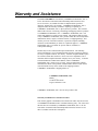
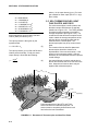
The surface layer (Figure 1.1-1) is comprised of
approximately the lower 10% of the atmospheric
boundary layer (ABL). The fluxes of water
vapor and heat within this layer are nearly
constant with height when the following criteria
are met: the surface has approximate
horizontal homogeneity; and the relationship z/h
<< 1 << z/zom is true, where zsfc is the height of
the surface layer, h is the height of the ABL, and
zom is the roughness length of momentum.
When the above conditions are met, the flux of
water vapor and heat, within the surface layer,
may be written as:
LE = L v w ′ρ′ v
(1)
H = ρa C p w ′ T ′
(2)
where LE is the latent heat flux, Lv is the latent
heat of vaporization, w′ is the instantaneous
deviation of vertical wind speed from the mean,
ρ′v is the instantaneous deviation of the water
vapor density from the mean, H is the sensible
heat flux, ρa is the density of air, Cp is the heat
capacity of air at a constant pressure, and T′ is
the instantaneous deviation of air temperature
from the mean (Stull, 1988).
The quantities w ′ T ′ and w ′ρ′ v are the
covariances between vertical wind speed and
temperature, and vertical wind speed and vapor
density. These quantities can be readily
calculated on-line by the datalogger.
The eddy covariance system directly measures
latent and sensible heat flux. If net radiation
and soil heat flux are also measured, energy
balance closure may be examined using the
surface energy balance equation:
Rn − G = H + LE
(3)
where Rn is the net radiation and G is the total
soil heat flux. H, LE, and G are defined as
positive away from the surface and Rn is
positive toward the surface.
FIGURE 1.1-1. Ideal Vertical Profiles of
Virtual Potential Temperature and Specific
Humidity Depicting All the Layers of the
Atmospheric Boundary Layer.
1.2 SYSTEM DESCRIPTION
1.2.1 SURFACE FLUX SENSORS
The eddy covariance system consists of three
sensors that measure the fluctuations in vertical
wind speed, air temperature, and water vapor
density. The CA27 is a one dimensional sonic
anemometer with a fine wire thermocouple
(127). The CA27 has a path length of 10 cm
and frequency response of 40 Hz. The 127 is a
12.7 µm fine wire thermocouple with a
frequency response of greater than 30 Hz. The
small size and symmetric construction of the
127 thermocouple junction minimizes radiation
loading (Tanner, 1979), thus it is not necessary
to shield the 127.
The KH20 is an ultraviolet krypton hygrometer
(Campbell and Tanner, 1985) which is similar in
principle to the Lyman-alpha hygrometer (Buck,
1976), except that the source tube contains
krypton gas. The KH20 has a frequency
response of 100 Hz.
1.2.1.1 Additional Required Measurements
Ambient air temperature and humidity must be
measured. This information is used to make
corrections to the water vapor measurements
and calculate air density.
1-1
SECTION 1. SYSTEM OVERVIEW
Wind direction must also be measured. The
wind direction is used to identify periods when
the mean wind was blowing over the back of the
eddy covariance sensors. Flux data from these
periods should not be used because of potential
flow distortions caused by the body and mounts
of the CA27 and KH20. A 75 degree sector
behind the sonic and hygrometer exists where
flow distortions may occur.
TABLE 1.2-1. Power Requirements for a
Typical Eddy Covariance Station
Sensor
CA27
KH20
21X
HMP35C
Current at 12
VDC unregulated
7 - 10 mA
10 - 20 mA
<25 mA
<5 mA
1.2.1.2 Optional Measurements
1.3 SYSTEM LIMITATIONS
When analyzing the surface flux data, it is often
useful to know the horizontal wind speed, along
with the wind direction. An estimate of friction
velocity and roughness length can be found
from the standard deviation of the vertical wind
speed and the mean horizontal wind speed,
during neutral conditions, e.g., H ≈ 0 (Panofsky
and Dutton, pp. 160, 1984).
1.3.1 RAIN
If net radiation and soil heat flux are measured
over the same period as the surface fluxes, a
check of energy balance closure may be made.
Net radiation is measured with a net radiometer.
Soil heat flux is measured by burying soil heat
flux plates at 8 cm. The average temperature
change of the soil layer above the plates is
measured with four parallel thermocouples.
The soil heat storage term is then found by
multiplying the change in soil temperature over
the averaging period by the total soil heat
capacity. The heat flux at the surface is the
sum of the measured heat flux at 8 cm and the
storage term. A measure of soil moisture is
required to find the total soil heat capacity. Soil
moisture can be found with the CS615 water
content reflectometer or by sampling.
1.2.2 POWER SUPPLY
The current requirements of a typical eddy
covariance station are given in Table 1.2-1. A
user-supplied 70 Amp hour battery will run the
system continuously for approximately two
months.
The CA27 uses unsealed transducers. Water
damages the transducers; protect the
transducers from rain and irrigation systems.
The 127 fine wire thermocouple junction is
extremely fragile. It may break if struck by
airborne debris, insects, or rain. Handle the 127
probes with care. Always store the 127 in a
127/ENC enclosure when not in use. Each
CA27 should have at least two 127s to minimize
system downtime due to a broken fine wire
thermocouple.
The seals on the hygrometer can be damaged
by prolonged exposure to extreme moisture,
e.g., rain. To avoid damage to the seals,
protect the hygrometer from rain.
In summary, do not allow the CA27, 127, and
KH20 to get wet.
1.3.2 SYSTEM SHUTDOWN
The eddy covariance system can be easily
protected from inclement weather with a plastic
bag. To avoid collecting meaningless data do
the following:
•
•
•
•
1-2
Set the execution interval to zero in the
table where the eddy covariance sensors
are being measured.
Remove the 127 and return it to a 127/ENC
enclosure.
Disconnect the power to the sonic and
hygrometer (to conserve battery power and
extend the life of the hygrometer tubes).
Cover the heads of the sonic and
hygrometer with a plastic bag.
SECTION 1. SYSTEM OVERVIEW
1.3.3 NO ABSOLUTE REFERENCE
The CA27 zero offset drifts with ambient air
temperature. The zero offset drift does not
effect the flux measurements, since only the
fluctuation about some mean are of interest.
This drift does, however, preclude the
measurement of the mean vertical wind speed.
The 127 does not measure absolute
temperature, instead the 127 is referenced to
the unknown temperature of the sonic base.
Thus, the output of the 127 is the difference
between the ambient air temperature and the
temperature of the sonic base. The reference
junction (CA27 base) has a thermal time
constant of approximately 20 minutes. To
extend the thermal time constant of the base,
insulate it with hot water pipe insulation.
Referencing the 127 to the sonic base does not
limit the ability of the 127 to measure
temperature fluctuations.
The window on the source tube of the
hygrometer is prone to scaling. This scaling is
caused by disassociation of atmospheric
constituents by the ultraviolet photons
(Campbell and Tanner, 1985). The rate of
scaling is a function of the atmospheric
humidity. In high humidity environments,
scaling can occur within a few hours. This
scaling attenuates the signal and can cause
shifts in the calibration curve. However, the
scaling over a typical flux averaging period is
small. Thus, water vapor fluctuation
measurements can still be made with the
hygrometer. The effects of the scaling can be
easily reversed by wiping the windows with a
moist swab.
1-3
SECTION 2. STATION INSTALLATION
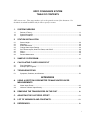
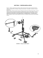
Figure 2-1 depicts a typical eddy covariance station that measures the latent and sensible heat flux,
ambient air temperature and humidity, wind speed and direction, net radiation, soil heat flux, and soil
temperature.
Point the eddy covariance sensors into the prevailing wind and the net radiometer to the south. The net
radiometer must be mounted far enough from any obstructions so that it is never shaded. Its field of
view should be representative of the surface where the flux measurements are being made. The net
radiometer can be mounted on a user-supplied stake or a CM6/CM10 tripod. The Tripod Weather
Station installation manual contains detailed instructions on installing the tripod and the meteorological
sensors.
FIGURE 2-1. Eddy Covariance Station
2-1
SECTION 2. STATION INSTALLATION
2.1 SENSOR HEIGHT
The eddy covariance sensors must be mounted
at some height that ensures that the
measurements are being made within the local
surface layer. The local surface layer grows at
a rate of approximately 1 vertical meter per 100
horizontal meters. Thus, a height to fetch
(horizontal distance traveled) ratio of 1:100 can
be used as a rough rule of thumb for determining the measurement height.
The following references discuss fetch
requirements in detail: Brutsaert (1986); Dyer
and Pruitt (1962); Gash (1986); Schuepp, et al.
(1990); and Shuttleworth (1992). The fetch
should be homogenous and flat, and no abrupt
changes in vegetation height should exist
(Tanner, 1988). Consider two adjacent fields,
the first planted with 1 m tall corn and the
second with 0.5 m soybean. Eddy covariance
sensors mounted at 2 m above the corn field
should have a minimum of 200 m of fetch in all
the directions that the data is of interest,
particularly between the eddy covariance
sensors and the interface between the corn and
soybean field.
2.2 MOUNTING
The CA27 and KH20 are shipped with a 0.75
inch by 0.75 inch NU-Rail (P/N 1017). The NURail is used to attach the horizontal mounting
arm to a 0.75 inch pipe vertical mast. The top
section of a CM6 tripod (Figure 2-1) can be
used as a horizontal cross arm mount. It can
be replaced with a longer threaded pipe if
necessary.
The CM6 leg separation can be adjusted to give
a measurement height of 1.1 m to 2.0 m. If the
desired measurement height is outside this
range, a CM10 or other user-supplied mounting
hardware will be required.
The CA27 must be mounted perpendicular to
the surface. This is done so that no horizontal
component of the wind is measured. In most
applications the surface is perpendicular to
gravity, thus the bubble level on the top of the
CA27 can be used to level the sensor.
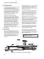
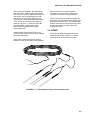
Mount the KH20 next to the CA27 with a
separation of 10 cm. The hygrometer should be
set back from the anemometer to minimize flow
distortions. Try to keep the hygrometer tubes
as far as possible from the fine wire
thermocouple. This is done to avoid measuring
temperature fluctuations caused by radiation
loading of the hygrometer tubes. Figure 2.2-1
depicts one possible mounting configuration.
Mount the KH20 so that the source tube (the
longer of the two tubes) is on top. Center the
path of the KH20 around the height of the fine
wire thermocouple on the CA27.
To mount the 127, place the 127 on the probe
arm located between the transducer arms.
Gently press and rotate the 127 until it slips into
place. To remove the 127, pull it horizontally
away from the CA27 base.
CAUTION: Do not twist the 127 once it is
seated on the mounting arm.
FIGURE 2.2-1. Top and Side View of the CA27 and KH20
2-2
SECTION 2. STATION INSTALLATION
FIGURE 2.2-2 CA27, KH20, HMP35C, and Wind Sentry Set On a CM6 Tripod
2.3 KH20 CALIBRATIONS
Each KH20 is calibrated over three different
vapor ranges. The vapor ranges are
summarized in Table 2.3-1. This calibration
may have been done under the following
conditions: windows scaled and clean, and at
sea level or 4500 ft (Logan, UT, 1372 m).
TABLE 2.3-1. KH20 Vapor Ranges
Range
Full
Dry
Wet
m-3
g
2 - 19
2 - 9.5
8.25 - 19
The Wet and Dry ranges will provide higher
resolution of vapor density fluctuations than the
Full Range. However, If the vapor range is
unknown or the vapor density is on the border
between Wet and Dry, then the Full range
should be used.
2.4 FINDING WATER VAPOR DENSITY
The ambient air temperature and relative humidity
are needed to calculate the vapor density. The
vapor density can then be used to determine the
correct vapor range to use on the KH20.
Before the KH20 is deployed in the field the
following decisions must be made:
From the ambient air temperature, the
saturation vapor pressure can be found using
the following sixth order polynomial:
•
e s = 0.1× a 0 + a1T + a 2 T + a3 T + a 4 T
•
•
Which calibrated elevation is most
appropriate for the site?
Will the windows be allowed to scale?
What vapor range is appropriate for the site?
Once those decisions are made, then the
appropriate -kw can be chosen from the KH20
calibration sheet. The path length (x) of the
KH20 is also given on each calibration sheet.
(
2
5
+a5 T + a6 T
6
)
3
4
(4)
where es is the saturation vapor pressure (kPa),
T is the ambient air temperature (K) (Lowe,
1977). The coefficients for Eq. (4) are given in
Table 2.4-1.
2-3
SECTION 2. STATION INSTALLATION
where ρv is the vapor density (g m-3), Rv is the
gas constant for water vapor (461.5 J K-1 kg-1)
(Stull, 1988).
TABLE 2.4-1 Polynomial Coefficients
a0 = 6984.505294
a1 = -188.9039310
a2 = 2.133357675
a3 = -1.288580973 x 10⁻²
a4 = 4.393587233 x 10⁻⁵
a5 = -8.023923082 x 10⁻⁸
a6 = 6.136820929 x 10⁻¹¹
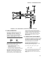
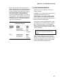
2.5 SOIL THERMOCOUPLES, HEAT
FLUX PLATES, AND CS615
The soil thermocouples, heat flux plates, and
the water content reflectometer are typically
installed as in Figure 2.5-1. The TCAV parallels
four thermocouples together to provide the
average temperature (see Figure 2.5-2). It is
constructed so that two thermocouples can be
used to obtain the average temperature of the
soil layer above one heat flux plate and the
other two above a second plate. The
thermocouple pairs may be up to two meters
apart.
Similar algorithms can be found in Goff and
Gratch (1946) and Weiss (1977).
The vapor pressure is then given by the
equation below.
e = 0.01 × RH × e s
(5)
The location of the two heat flux plates and
thermocouples should be chosen to be
representative of the area under study. If the
ground cover is extremely varied, it may be
necessary to have additional sensors to provide
a valid average.
The vapor pressure (e) is in kPa and RH is the
relative percent humidity. Finally, the water
vapor density is found with the following:
ρv =
e∗10 6
TR v
(6)
Up to 1
Use a small shovel to make a vertical slice in
the soil and excavate the soil to one side of the
slice. Keep this soil intact so that it may be
replaced with minimal disruption.
m
2.5 cm
2 cm
Ground
6 cm
8 cm
Partial emplacement of the HFT3 and TCAV
sensors is shown for illustration purposes. All
sensors must be completely inserted into the soil
face before the hole is backfilled.
FIGURE 2.5-1. Placement of Thermocouples and Heat Flux Plates
2-4
Surfac
e
SECTION 2. STATION INSTALLATION
The sensors are installed in the undisturbed
face of the hole. Measure the sensor depths
from the top of the hole. Make a horizontal cut,
with a knife, into the undisturbed face of the
hole and insert the heat flux plates into the
horizontal cut. Press the stainless steel tubes
of the TCAVs above the heat flux plates as
shown in Figure 2.5-1. Be sure to insert the
tube horizontally. When removing the
thermocouples, grip the tubing, not the
thermocouple wire.
Install the CS615 as shown in Figure 2.5-1.
See the CS615 manual (Section 5) for detailed
installation instructions.
back from the hole to minimize thermal
conduction on the lead wires. Replace the
excavated soil back to its original position.
Finally, wrap the end of the thermocouple wire
around the 21X base at least twice before wiring
them into the terminal strip. This will minimize
thermal conduction into the terminal strip. After
all the connections are made, replace the
terminal strip cover.
2.6 WIRING
The CA27 and KH20 are shipped with 25 ft
standard lead lengths. Table 2.6-1 lists the
connections for the CA27 and the KH20.
Never run the leads directly to the surface.
Rather, bury the sensor leads a short distance
FIGURE 2.5-2. TCAV Spatial Averaging Thermocouple Probe
2-5
SECTION 2. STATION INSTALLATION
TABLE 2.6-1. CA27 and KH20 Sensor Lead
Color Assignments
Sensor
CA27 Wind +
CA27 Wind CA27 Shield
CA27 Temperature +
CA27 Temperature CA27 +12 V
CA27 Power Gnd
KH20 Water Vapor +
KH20 Water Vapor KH20 Shield
KH20 +12 V
KH20 Power Gnd
Color
Green
Black
Clear
White
Black (same as Wind-)
Red
Black of Red and Black
White
Black
Clear
Red
Black of Red and Black
Tables 2.6-2 and 2.7-1 list the connections to
the 21X for the example program in Section 3.
The following sensors are measured in the
example:
•
CA27 (vertical wind speed and temperature
fluctuations)
KH20 (water vapor density fluctuations)
Q7 (net radiation)
HFT3 (soil heat flux)
TCAV (soil temperature)
HMP35C (ambient air temperature and
relative humidity)
03001 (wind speed and direction)
CS615 (soil moisture)
•
•
•
•
•
•
•
5H
5L
GND
HMP35C (air temp)
HMP35C (humidity)
Ground/Shield
Orange
Green
White/Clear
6H
6L
GND
HTF1 #1 (soil heat flux)
Black
HTF1 #2 (soil heat flux)
Black
Ground/Shield
White/Clear
Ground/Shield
White/Clear
7H
7L
GND
Not used
03001 (wind direction)
03001 Ground/Shield
8H
8L
GND
Q7 + (net radiation)
Q7 - (net radiation)
Shield
Red
Black
Clear
1EX
2EX
1C
GND
2C
HMP35C (temp)
03001 (wind direction)
HMP35C (turn unit on)
HMP35C (power ground)
CS615 (turn unit on)
Black
Black
Yellow
Purple
Orange
1P
GND
2P
GND
03001 (wind speed)
Black
Ground/Shield
White/Clear
CS615 (soil water content) Green
Ground/Shield
Black/Clear
+12
+12
GND
HMP35C
Red
CS615
Red
To the common earth ground
Red
White/Clear
2.7 POWER
TABLE 2.6-2. 21X/Sensor Connections for
Example Program
Channel
Sensor
Color
1H
1L
GND
CA27 + (wind)
CA27 - (wind/temp)
Shield
Green
Black
Clear
2H
2L
GND
CA27 + (temp)
jumper to 1L
White
3H
3L
GND
KH20 + (vapor)
KH20 - (vapor)
Shield
White
Black
Clear
4H
4L
GND
TCAV + (soil temp)
TCAV - (soil temp)
Purple
Red
2-6
The CA27 and KH20 are powered by an
external battery. A user-supplied 70 Ahr deep
cycle RV battery will run the system for
approximately two months. The CA27 and
KH20 power cables are connected directly to
the battery terminals. Disconnect the power
cables when the system is not collecting data,
e.g. during a rain shower.
Power the 21X from the external battery. Table
2.7-1 summarizes the power connections.
NOTE: If the 21X is powered by an
external battery, it must have a blocking
diode in the supply line from its internal
batteries to prevent reverse charging of the
alkaline cells by the external battery. This
diode has been standard on all 21Xs
shipped since January 19, 1987. If an
earlier 21X is being used, either add the
diode (contact Campbell Scientific for
details) or turn off the 21X power switch
while the external battery is connected.
SECTION 2. STATION INSTALLATION
Be sure the 21X has a good earth ground, to
protect against primary and secondary lightning
strikes. The purpose of an earth ground is to
minimize damage to the system by providing a
low resistance path around the system to a
point of low potential. Campbell Scientific
recommends that all dataloggers in the field be
earth grounded. All components of the system
(datalogger, sensors, external power supplies,
mounts, housing, etc.) should be referenced to
one common earth ground.
TABLE 2.7-1. External Battery Connections
for Example Program
Terminal
Sensor
Color
Pos (+)
CA27 (power)
KH20 (power)
21X (+12, see note)
Red
Red
User
Supplied
CA27 (power)
KH20 (power)
21X (ground)
Black
Black
User
Supplied
Neg (-)
2.8 ROUTINE MAINTENANCE
Check the 127 on a daily basis. If the 127 is
broken, replace it.
Inspect the 127 for spider webs. Carefully blow
away any spider webs with a can of
compressed air. Do not put the thermocouple
junction directly in the air stream from the can
because the junction may break. Direct the air
stream to the side of the junction.
If the system is running “windows clean”, clean
the windows with a moistened swab. Set flag 1
high to disable averaging. Use only distilled
water to moisten the swab. With a fresh swab,
dry the windows after cleaning. Set flag 1 low to
resume averaging.
CAUTION: Never look directly into the
KH20 source tube (the larger of the two
tubes).
Check the net radiometer domes for dirt and
debris. A camel’s hair brush, with bellows for
blowing off dust particles such as those used in
cleaning photographic negatives, can be used
without fear of scratching the domes.
2-7
SECTION 3. SAMPLE 21X PROGRAM
This section provides a sample program that may be used to measure the eddy covariance sensors and
the auxiliary sensors. The CA27, 127, and KH20 are measured in Table 1 at 5 Hz. The meteorological
sensors and the energy balance sensors are measured in Table 2 at 0.5 Hz. The meteorological
sensors include wind speed, wind direction, air temperature, and vapor pressure. The energy balance
sensors include net radiation, soil heat flux soil temperature, soil water content, and change in soil
temperature. Note that even if this exact installation is used, the correct multipliers must be entered for
the net radiometer and soil heat flux plate.
The execution interval in Table 1 may be changed to 0.1 (10 Hz). For most flux studies the increased
sample rate does not add any significant statistical information about the turbulent fluxes. It does,
however, increase the current drain of the datalogger and cause Table 1 to overrun every ten minutes
when the subinterval averages are calculated. If the execution interval is changed to 0.1, the seventh
parameter in the twelfth instruction (P62) must be changed to 6000.
To conserve battery power and extend the life of the krypton hygrometer tubes, disconnect the CA27
and KH20 from the battery when measurements are not being made, e.g., during a rain shower. During
a rain shower or other inclement weather, shut down and cover the eddy correction system with plastic
bags (see Section 1.3.1 for details).
Set flag 1 high to disable averaging while cleaning the KH20 windows and performing other station
maintenance. Set flag 1 low to resume averaging.
;{21X}
;
;c:\dl\ec\ecsep96.csi
;5 September 1996
;
*Table 1 Program
01:
0.2
Execution Interval (seconds)
01:
If Flag/Port (P91)
1:
22
Do if Flag 2 is Low
2:
2
Call Subroutine 2
02:
Volt (Diff) (P2)
1:
3
2:
15
3:
1
4:
1
5:
1
6:
0
Reps
5000 mV Fast Range
In Chan
Loc [ w
]
Mult
Offset
Z=X*F (P37)
1:
1
2:
.001
3:
1
X Loc [ w
F
Z Loc [ w
Z=X*F (P37)
1:
2
2:
.004
3:
2
X Loc [ T
F
Z Loc [ T
03:
04:
]
]
]
]
;Move new signal before natural log.
3-1
SECTION 3. SAMPLE 21X PROGRAM
;
05:
Z=X (P31)
1:
3
2:
4
;Copy KH20 output.
;
06: Z=X (P31)
1:
3
2:
5
07:
Z=LN(X) (P40)
1:
3
2:
3
X Loc [ lnVh
Z Loc [ Vh
]
]
X Loc [ lnVh
]
Z Loc [ Vh_mV ]
X Loc [ lnVh
Z Loc [ lnVh
]
]
;Subtract a constant.
;
08: Z=X-Y (P35)
1:
3
2:
23
3:
3
X Loc [ lnVh
Y Loc [ lnVho
Z Loc [ lnVh
]
]
]
;Subtract a constant.
;
09: Z=X-Y (P35)
1:
4
2:
24
3:
4
X Loc [ Vh
Y Loc [ Vho
Z Loc [ Vh
]
]
]
;Set Flag 1 high while cleaning KH20 windows.
;
10: If Flag/Port (P91)
1:
11
Do if Flag 1 is High
2:
19
Set Flag 9 High
11:
If time is (P92)
1:
0
2:
30
3:
10
Minutes into a
Minute Interval
Set Output Flag High
;Ten minute subinterval average.
;10 min/avg period = (3000 smpls/avg period / (5 smpls/sec * 60 sec/min).
;
12: CV/CR (OSX-0) (P62)
1:
4
No. of Input Locations
2:
4
No. of Means
3:
4
No. of Variances
4:
0
No. of Std. Dev.
5:
4
No. of Covariance
6:
0
No. of Correlations
7: 3000
Samples per Average
8:
1
First Sample Loc [ w
]
9:
10
Loc [ avg_w ]
3-2
SECTION 3. SAMPLE 21X PROGRAM
13:
If Flag/Port (P91)
1:
10
Do if Output Flag is High (Flag 0)
2:
30
Then Do
;(w'T')rhoCp = H
;
14: Z=X*Y (P36)
1:
18
2:
27
3:
18
X Loc [ H
]
Y Loc [ rhoCp ]
Z Loc [ H
]
;[w'(lnVh)']Lv/-xkw = LE
;
15: Z=X/Y (P38)
1:
19
X Loc [ LE
]
2:
26
Y Loc [ neg_xkw ]
3:
19
Z Loc [ LE
]
16:
Z=X*Y (P36)
1:
19
2:
28
3:
19
X Loc [ LE
Y Loc [ Lv
Z Loc [ LE
]
]
]
;Add constant to average.
;
17: Z=X+Y (P33)
1:
12
X Loc [ avg_lnVh ]
2:
23
Y Loc [ lnVho ]
3:
12
Z Loc [ avg_lnVh ]
;Add constant to average.
;
18: Z=X+Y (P33)
1:
13
X Loc [ avg_Vh ]
2:
24
Y Loc [ Vho
]
3:
13
Z Loc [ avg_Vh ]
;Save new constant.
;
19: Z=LN(X) (P40)
1:
5
2:
23
X Loc [ Vh_mV ]
Z Loc [ lnVho ]
;Save new constant.
;
20: Z=X (P31)
1:
5
2:
24
X Loc [ Vh_mV ]
Z Loc [ Vho
]
21:
End (P95)
22:
If Flag/Port (P91)
1:
10
Do if Output Flag is High (Flag 0)
2:
10
Set Output Flag High
3-3
SECTION 3. SAMPLE 21X PROGRAM
23:
Set Active Storage Area (P80)
1:
1
Final Storage
2:
12
Array ID
24:
Resolution (P78)
1:
0
low resolution
25:
Real Time (P77)
1: 0110
Day,Hour/Minute
26:
Resolution (P78)
1:
1
high resolution
27:
Sample (P70)
1:
4
2:
25
Reps
Loc [ neg_kw
Sample (P70)
1:
10
2:
10
Reps
Loc [ avg_w
Sample (P70)
1:
1
2:
21
Reps
Loc [ T_lnVh_ ]
28:
29:
30:
]
]
Serial Out (P96)
1:
30
SM192/SM716/CSM1
*Table 2 Program
01:
2.0
Execution Interval (seconds)
01:
If Flag/Port (P91)
1:
23
Do if Flag 3 is Low
2:
3
Call Subroutine 3
02:
Temp 107 Probe (P11)
1:
1
Reps
2:
9
In Chan
3:
1
Excite all reps w/Exchan 1
4:
41
Loc [ Tair
]
5:
1
Mult
6:
0
Offset
03:
Volts (SE) (P1)
1:
1
2:
5
3:
10
4:
48
5:
.001
6:
0
04:
3-4
Reps
5000 mV Slow Range
In Chan
Loc [ RH_frac ]
Mult
Offset
Saturation Vapor Pressure (P56)
1:
41
Temperature Loc [ Tair
2:
42
Loc [ e
]
]
SECTION 3. SAMPLE 21X PROGRAM
05:
06:
Z=X*Y (P36)
1:
42
2:
48
3:
42
X Loc [ e
]
Y Loc [ RH_frac ]
Z Loc [ e
]
Volts (SE) (P1)
1:
2
2:
2
3:
11
4:
43
5:
1
6:
0
Reps
15 mV Slow Range
In Chan
Loc [ SHF#1 ]
Mult
Offset
;Enter multiplier for SHF#1 (mult#1).
;
07: Z=X*F (P37)
1:
43
X Loc [ SHF#1
F
2: mult#1
3:
43
Z Loc [ SHF#1
]
]
;Enter multiplier for SHF#2 (mult#2).
;
08: Z=X*F (P37)
1:
44
X Loc [ SHF#2
F
2: mult#2
3:
44
Z Loc [ SHF#2
09:
10:
]
]
Volt (Diff) (P2)
1:
1
2:
4
3:
8
4:
45
5:
1
6:
0
Reps
500 mV Slow Range
In Chan
Loc [ Rnet
]
Mult
Offset
IF (X<=>F) (P89)
1:
45
2:
3
3:
0
4:
30
X Loc [ Rnet
>=
F
Then Do
]
;Apply positive wind correction to Rnet.
;
11: Do (P86)
1:
4
Call Subroutine 4
12:
Else (P94)
;Apply negative wind correction to Rnet.
;
13: Do (P86)
1:
5
Call Subroutine 5
14:
End (P95)
3-5
SECTION 3. SAMPLE 21X PROGRAM
15:
16:
17:
Pulse (P3)
1:
1
2:
1
3:
21
4:
49
5:
.75
6:
.2
Reps
Pulse Input Chan
Low Level AC, Output Hz
Loc [ WndSpd ]
Mult
Offset
IF (X<=>F) (P89)
1:
49
2:
1
3:
.2
4:
30
X Loc [ WndSpd
=
F
Then Do
Z=F (P30)
1:
0
2:
49
F
Z Loc [ WndSpd
]
]
18:
End (P95)
19:
AC Half Bridge (P5)
1:
1
Reps
2:
5
5000 mV Slow Range
3:
14
In Chan
4:
2
Excite all reps w/Exchan 2
5: 5000
mV Excitation
6:
50
Loc [ WndDir ]
7:
355
Mult
8:
0
Offset
20:
Internal Temperature (P17)
1:
40
Loc [ RefTemp ]
21:
Thermocouple Temp (DIFF) (P14)
1:
1
Reps
2:
1
5 mV Slow Range
3:
4
In Chan
4:
2
Type E (Chromel-Constantan)
5:
40
Ref Temp Loc [ RefTemp ]
6:
46
Loc [ Tsoil ]
7:
1
Mult
8:
0
Offset
;Turn on CS615 soil moisture probe
;once every half hour.
;
22: If time is (P92)
1:
14
Minutes into a
2:
30
Minute Interval
3:
14
Set Flag 4 High
23:
3-6
If Flag/Port (P91)
1:
14
Do if Flag 4 is High
2:
30
Then Do
SECTION 3. SAMPLE 21X PROGRAM
24:
Do (P86)
1:
42
Set Port 2 High
;Measure CS615 soil moisture probe.
;When the CS615 is off (Flag 4 low),
;Input Locations CS615_ms and soil_wtr
;will not change.
;
25: Pulse (P3)
1:
1
Reps
2:
2
Pulse Input Channel
3:
21
Low Level AC, Output Hz
4:
52
Loc [ CS615_ms ]
5:
.001
Mult
6:
0
Offset
26:
27:
28:
Z=1/X (P42)
1:
52
2:
52
X Loc [ CS615_ms ]
Z Loc [ CS615_ms ]
Polynomial (P55)
1:
1
2:
52
3:
53
4:
-.187
5:
.037
6:
.335
7:
0
8:
0
9:
0
Reps
X Loc [ CS615_ms ]
F(X) Loc [ soil_wtr ]
C0
C1
C2
C3
C4
C5
End (P95)
;Turn CS615 probe off.
;
29: If time is (P92)
1:
15
Minutes into a
2:
30
Minute Interval
3:
30
Then Do
30:
31:
Do (P86)
1:
24
Set Flag 4 Low
Do (P86)
1:
52
Set Port 2 Low
32:
End (P95)
33:
If time is (P92)
1:
0
2:
30
3:
10
34:
Minutes into a
Minute Interval
Set Output Flag High
Set Active Storage Area (P80)
1:
3
Input Storage
2:
46
Array ID or Loc [ Tsoil
]
3-7
SECTION 3. SAMPLE 21X PROGRAM
35:
Average (P71)
1:
1
2:
46
Reps
Loc [ Tsoil
]
36:
If Flag/Port (P91)
1:
10
Do if Output Flag is High (Flag 0)
2:
30
Then Do
37:
Z=X-Y (P35)
1:
46
2:
51
3:
47
X Loc [ Tsoil ]
Y Loc [ Prev_Ts ]
Z Loc [ del_Tsoil ]
Z=X (P31)
1:
46
2:
51
X Loc [ Tsoil ]
Z Loc [ Prev_Ts ]
38:
;Apply temperature correction to soil
;moisture data measured by the CS615.
;
39: Z=X+F (P34)
1:
46
X Loc [ Tsoil ]
2:
-20
F
3:
31
Z Loc [ I
]
40:
41:
42:
43:
44:
3-8
Polynomial (P55)
1:
1
2:
53
3:
32
4:
-.0346
5:
1.9
6:
-4.5
7:
0
8:
0
9:
0
Reps
X Loc [ soil_wtr ]
F(X) Loc [ J
]
C0
C1
C2
C3
C4
C5
Z=X*F (P37)
1:
32
2:
.01
3:
32
X Loc [ J
F
Z Loc [ J
]
Z=X*Y (P36)
1:
31
2:
32
3:
31
X Loc [ I
Y Loc [ J
Z Loc [ I
]
]
]
Z=X-Y (P35)
1:
53
2:
31
3:
54
X Loc [ soil_wtr ]
Y Loc [ I
]
Z Loc [ soil_w_T ]
End (P95)
]
SECTION 3. SAMPLE 21X PROGRAM
45:
If Flag/Port (P91)
1:
10
Do if Output Flag is High (Flag 0)
2:
10
Set Output Flag High
46:
Set Active Storage Area (P80)
1:
1
Final Storage
2:
21
Array ID
47:
Resolution (P78)
1:
0
low resolution
48:
Real Time (P77)
1: 0110
Day,Hour/Minute
49:
Resolution (P78)
1:
1
high resolution
50:
Average (P71)
1:
6
2:
40
Reps
Loc [ RefTemp ]
Sample (P70)
1:
3
2:
46
Reps
Loc [ Tsoil
51:
]
52:
Wind Vector (P69)
1:
1
Reps
2:
300
Samples per Sub-Interval
3:
0
S, θu, & σ(θu) Polar
4:
49
Wind Speed/East Loc [ WndSpd ]
5:
50
Wind Direction/North Loc [ WndDir ]
53:
Sample (P70)
1:
3
2:
52
Reps
Loc [ CS615_ms ]
*Table 3 Subroutines
01:
Beginning of Subroutine (P85)
1:
2
Subroutine 2
02:
Do (P86)
1:
12
Set Flag 2 High
;Enter -kw for hygrometer
;
03: Z=F (P30)
-kw
F
1:
2:
25
Z Loc [ neg_kw
]
;Enter -xkw for hygrometer
;
04: Z=F (P30)
-xkw
F
1:
2:
26
Z Loc [ neg_xkw ]
3-9
SECTION 3. SAMPLE 21X PROGRAM
05:
06:
Z=F (P30)
1: 1010
2:
27
F
Z Loc [ rhoCp
Z=F (P30)
1: 2440
2:
28
F
Z Loc [ Lv
]
]
;Measure constant for first pass.
;
07: Volt (Diff) (P2)
1:
1
Reps
2:
15
5000 mV Fast Range
3:
3
In Chan
4:
24
Loc [ Vho
]
5:
1
Mult
6:
0
Offset
;Constant for first pass.
;
08: Z=LN(X) (P40)
1:
24
X Loc [ Vho
2:
23
Z Loc [ lnVho
09:
Do (P86)
1:
10
]
]
Set Output Flag High
10:
Set Active Storage Area (P80)
1:
1
Final Storage
2:
11
Array ID
11:
Resolution (P78)
1:
0
low resolution
12:
Real Time (P77)
1: 0110
Day,Hour/Minute
13:
Resolution (P78)
1:
1
high resolution
14:
Sample (P70)
1:
4
2:
25
Reps
Loc [ neg_kw
15:
End (P95)
16:
Beginning of Subroutine (P85)
1:
3
Subroutine 3
17:
Do (P86)
1:
13
Set Flag 3 High
;Turn on RH portion of the HMP35C.
;
18: Do (P86)
1:
41
Set Port 1 High
3-10
]
SECTION 3. SAMPLE 21X PROGRAM
19:
Internal Temperature (P17)
1:
40
Loc [ RefTemp ]
;Prev_Ts for first pass.
;
20: Thermocouple Temp (DIFF) (P14)
1:
1
Reps
2:
1
5 mV Slow Range
3:
4
In Chan
4:
2
Type E (Chromel-Constantan)
5:
40
Ref Temp Loc [ RefTemp ]
6:
51
Loc [ Prev_Ts ]
7:
1
Mult
8:
0
Offset
21:
End (P95)
22:
Beginning of Subroutine (P85)
1:
4
Subroutine 4
23:
Z=X*F (P37)
1:
49
2:
.2
3:
37
X Loc [ WndSpd
F
Z Loc [ C
]
Z=X*F (P37)
1:
37
2:
.066
3:
35
X Loc [ C
F
Z Loc [ A
Z=X+F (P34)
1:
37
2:
.066
3:
36
X Loc [ C
F
Z Loc [ B
Z=X/Y (P38)
1:
35
2:
36
3:
38
X Loc [ A
]
Y Loc [ B
]
Z Loc [ CorrFact ]
Z=Z+1 (P32)
1:
38
Z Loc [ CorrFact ]
24:
25:
26:
27:
;Enter the positive multiplier (p.ppp).
;
28: Z=X*F (P37)
1:
45
X Loc [ Rnet
p.ppp
F
2:
3:
45
Z Loc [ Rnet
29:
Z=X*Y (P36)
1:
45
2:
38
3:
45
]
]
]
]
]
]
]
X Loc [ Rnet
]
Y Loc [ CorrFact ]
Z Loc [ Rnet
]
3-11
SECTION 3. SAMPLE 21X PROGRAM
30:
End (P95)
31:
Beginning of Subroutine (P85)
1:
5
Subroutine 5
32:
Z=X*F (P37)
1:
49
X Loc [ WndSpd
2:
.00174 F
3:
35
Z Loc [ A
]
33:
Z=X+F (P34)
1:
35
X Loc [ A
]
2:
.99755 F
3:
38
Z Loc [ CorrFact ]
;Enter the negative multiplier (n.nnn).
;
34: Z=X*F (P37)
1:
45
X Loc [ Rnet
n.nnn
F
2:
3:
45
Z Loc [ Rnet
35:
36:
]
Z=X*Y (P36)
1:
45
2:
38
3:
45
]
]
X Loc [ Rnet
]
Y Loc [ CorrFact ]
Z Loc [ Rnet
]
End (P95)
End Program
*
01:
02:
A
56
64
-Input Locations1w
2T
3 lnVh
4 Vh
5 Vh_mV
6 _________
7 _________
8 _________
9 _________
10 avg_w
11 avg_T
12 avg_lnVh
13 avg_Vh
14 var_w
3-12
Mode 10 Memory Allocation
Input Location
Intermediate Locations
15 var_T
16 var_lnVh
17 var_Vh
18 H
19 LE
20 w'Vh'
21 T'(lnVh)'
22 _________
23 lnVho
24 Vho
25 -kw
26 -xkw
27 rhoCp
28 Lv
29 _________
30 _________
31 _________
32 _________
33 _________
34 _________
35 A
36 B
37 C
38 CorrFact
39 _________
40 RefTemp
41 Tair
42 e
43 SHF#1
44 SHF#2
45 Rnet
46 Tsoil
47 del_Tsoil
48 RH_frac
49 WndSpd
50 WndDir
51 Prev_Ts
52 _________
53 _________
54 _________
55 _________
56 _________
SECTION 3. SAMPLE 21X PROGRAM
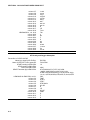
TABLE 3.1-1. Output from Example Eddy Covariance Program
01:
02:
03:
04:
05:
06:
07:
ID = 11; compile time and constants
DAY
Time(hhmm)
-kw (m3 g-1 cm-1)
-xkw (m3 g-1)
air density x heat capacity (W m-2 K-1 m-1 s)
latent heat of vaporization (J g-1)
01:
02:
03:
04:
05:
06:
07:
08:
09:
10:
11:
12:
13:
14:
15:
16:
17:
ID = 12; surface flux data
DAY
Time (hhmm)
-kw (m3 g-1 cm-1)
-xkw (m3 g-1)
air density x heat capacity (W m-2 K-1 m-1 s)
latent heat of vaporization (J g-1)
average vertical wind speed (m s-1)
average CA27 temperature (°C)
average natural log of KH20 (unit less)
average voltage from KH20 (mV)
variance of the vertical wind speed (m s-1)
variance of the CA27 temperature (°C)
variance of the natural log of KH20 voltage (unit less)
variance of the voltage from KH20 (mV)
sensible heat flux (W m-2)
latent heat flux (W m-2)
′
′
18: T ln Vh ; used in oxygen correction for variance of water vapor density
(
01:
02:
03:
04:
05:
06:
07:
08:
09:
10:
11:
12:
13:
14:
15:
16:
17:
18:
)
ID = 21; meteorological and energy balance data
DAY
Time (hhmm)
average panel temperature (°C)
average ambient air temperature (°C)
average vapor pressure (kPa)
average soil heat flux #1 (W m-2)
average soil heat flux #2 (W m-2)
average net radiation (W m-2)
average soil temperature (°C)
change in soil temperature (°C)
sample RH (fraction)
average wind speed (m s-1)
unit vector wind direction (deg)
standard deviation of wind direction (deg)
CS615 period (msec)
soil water content (fraction)
soil water content corrected for soil temperature (fraction)
3-13
SECTION 4. CALCULATING FLUXES USING SPLIT
SPLIT (PC208E software) can be used to apply the air density and oxygen corrections to the measured
surface fluxes. This section provides example SPLIT programs to make the necessary calculations on
the data produced by the sample datalogger program. All the calculations in ECRAW.PAR and
ECFLUX.PAR are explained in Sections 1 and Appendix A.
Two runs through SPLIT are required to combine the data and then apply the corrections. The first run
operates on the raw data produced by the datalogger. The parameter file ECRAW.PAR is used to make
the first run and produces the file called EC.PRN. The second run is made with the parameter file
ECFLUX.PAR. This parameter file corrects the air density and applies the necessary oxygen correction
to the data. The output file name is FLUX.PRN. To apply the oxygen correction (OCLE) to the latent
heat flux, subtract OCLE from LE (see Eq. 14 and 15). To apply the oxygen correction to the standard
deviation of water vapor, add OCSD to STDR.
4.1 FLUX CALCULATIONS
The surface flux data is combined with the
energy balance and meteorological data. The
SPLIT parameter file that does this is listed in
TABLE 4.2-1. The parameter file assumes that
the data files from the datalogger were saved
on disk under the name EC.DAT. An output
data file (EC.PRN) is created that will be used
to apply all the necessary corrections.
4.2 EXAMPLE SPLIT PROGRAMS
Table 4.2-2 lists the parameter file that is used
to apply the corrections. The equations that
ECFLUX.PAR uses are described in detail in
Section 1 and Appendix A. Appendix D
summarizes the variable names and definitions.
In some cases it may be necessary to apply an
additional correction to the latent heat flux
(Webb et al., 1980). The soil storage term and
the heat capacity of soil was found following
Hanks and Ashcroft, 1980. Soil water content
(W) is measured by the CS615. Bulk density
(BD) is unique for each site and must be
measured for the site. An estimate for
atmosphere pressure (P) must also be entered.
TABLE 4.2-1. Split Parameter File to Combine Raw Data
Param file is C:\ECRAW.PAR
Name(s) or input DATA FILE(s):
Name of OUTPUT FILE to generate:
START reading in EC.DAT:
START reading in:
STOP reading in EC.DAT:
STOP reading in:
COPY from EC.DAT:
COPY from:
SELECT element #(s) in EC.DAT:
SELECT element #(s) in:
HEADING for report:
HEADINGS for EC.DAT, col # 1:
column # 2:
column # 3:
column # 4:
column # 5:
column # 6:
EC.DAT, EC.DAT
EC.PRN
2:3
2:3
1[12] AND 3[30]
1[21] AND 3[30]
2..5,P = 85.,P,6..11,SQRT(12..15),16..18
BD=1330.,W =18,LV=(2500.5-2.359*5),
TA=5+273.15,Q=(.622*6)/(P-(6*1.622)),
CP=(1.+(.87*Q))*1005.,RD=(P-6)*1000./
(287.04*TA),RV=6*1000./(461.5*TA),RA=RD+
RV,F=SPAAVG(7,8),S=11*.08*BD*(840.+
W*4190.)/1800.,TA,6,9,F,S,12..14,LV,CP,RA
RAW EDDY COVARIANCE DATA
DAY
TIME
-kw
-xkw
P
rhoCp
4-1
SECTION 4. CALCULATING FLUXES USING SPLIT
column # 7:
column # 8:
column # 9:
column # 10:
column # 11:
column # 12:
column # 13:
column # 14:
column # 15:
column # 16:
column # 17:
column # 18:
HEADINGS for , col. # 19:
column # 20:
column # 21:
column # 22:
column # 23:
column # 24:
column # 25:
column # 26:
column # 27:
column # 28:
column # 29:
Lv old
avg w
avg T
avg InV
avg Vh
std w
std T
std InV
std Vh
H
LE
T′InV′
Tair
e
Rn
F
S
ws
wd
sd wd
Lv new
Cp
rho air
TABLE 4.2-2. Split Parameter File to Correct Surface Fluxes for
Air Density and Oxygen Absorption
Param file is C:\ECFLUX.PAR
Name(s) or input DATA FILE(s):
Name of OUTPUT FILE to generate:
START reading in ENC.PRN:
STOP reading in ENC.PRN:
COPY from ENC.PRN:
SELECT element #(s) in ENC.PRN:
HEADINGS for ENC.PRN, col # 1:
column # 2:
column # 3:
column # 4:
column # 5:
column # 6:
column # 7:
column # 8:
column # 9:
column # 10:
column # 11:
column # 12:
column # 13:
4-2
EC.PRN
FLUX.PRN
1:2
2[30]
H=16*28*29/6,LE=17*27/7,A=5*1000.
*.80674*.0045,OCLE=16*A*27/(3*6*19*19),
STDR=14/4,OCSD=SQRT(((2.*A*18/(3*4*19*19)))),
1,2,12,13,STDR,OCSD,H,LE,OCLE,21,22+23,22,23
DAY
TIME
STD w
STD T
STD RHOV
OC SD
H
LE
OC LE
RNET
G
F
S
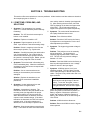
SECTION 5. TROUBLESHOOTING
This section offers some solutions to common problems. All the locations and data values are based on
the example program in Section 3.
5.1 SYMPTOMS, PROBLEMS, AND
SOLUTIONS
1. Symptom: The temperature is a constant
value of 17, with the fractional portion randomly
fluctuating.
Problem: The 127 fine wire thermocouple is
broken or not installed.
Solution: Replace or install the 127.
2. Symptom: Signal response on the 127 is
down. Input location 2 data is fluctuating slowly.
Problem: Debris is caught up in the fine wire
thermocouple junction, e.g. a spider web.
Solution: Carefully blow away the debris with a
can of compressed air. Do not direct the air
stream at the thermocouple junction because
the junction is extremely fragile. Rather, put the
junction on the peripheral of the air stream.
3. Symptom: The vertical wind is fluctuating only
in the hundredths place. When the transducers
are blown on, the CA27 does not respond with
reasonable values.
Problem: One or more transducers are
missing or the transducer pins have been
damaged.
Solution: Replace the transducers, see
Appendix B for removal and installation
procedures.
4. Symptom: Vertical wind speed is a near
steady positive or negative value.
Problem: A transducer is shorted. The
transducers will short if they are twisted on the
mounting arms (see Appendix B for proper
removal procedure) or if they become wet.
When the transducers are shorted, the CA27
outputs a near constant voltage. If the lower
transducer is shortened, the CA27 will output a
negative value. If the upper transducer is
shorted, the CA12 will output a positive value.
Solution: Allow the transducers several hours
to dry. Then check the CA27 zero offset with a
zero velocity anechoic chamber (see Appendix
C). After checking the zero offset, check the
CA27 by blowing on the lower and upper arms
of the CA27. The 21X should measure a
negative and positive wind speed respectively.
5. Symptom: The vertical wind fluctuations are
not equally distributed around zero.
Problem: Zero offset has drifted.
Solution: Send the CA27 back to the factory
for adjustment or see Appendix C for the zero
offset adjustment procedures.
6. Symptom: The krypton hygrometer voltage is
-99999.
Problem: This problem occurs in extremely
arid environments. The hygrometer is
outputting signal greater than 5 Volts to the
21X. The 21X can only measure voltages
between ± 5 Volts.
Solution: Send the KH20 back to the factory to
have its path length widened or use a voltage
divider to reduce in the input signal.
7. Symptom: KH20 has power, but it is not
outputting a signal. The “blue glow” from the
source tube (the larger of the two tubes) is not
visible. The glow is only visible under low or no
light conditions.
CAUTION: Never look directly into the
KH20 source tube (the longer of the two
tubes). To see the “blue glow”, insert a
piece of paper between the tubes, under
low light conditions, and look at the paper.
When an Ammeter is placed serially in the
power line (positive of Ammeter to positive of
battery, negative of Ammeter to positive of
KH20, and negative of KH20 to negative of
battery), the current drain is not in the range of
10 to 20 mA.
Problem: KH20 tubes have blown out.
Solution: Return the KH20 to have the krypton
tubes replaced.
5-1
APPENDIX A. USING A KRYPTON HYGROMETER TO MAKE
WATER VAPOR MEASUREMENTS
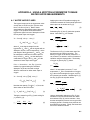
A.1 WATER VAPOR FLUXES
The krypton lamp used in the hygrometer emits
a major line at 123.58 nm (line 1) and a minor
line at 116.49 nm (line 2). Both of these
wavelengths are absorbed by water vapor and
oxygen. The equation below describes the
hygrometer signal in terms of absorption of both
lines by water vapor and oxygen.
(
Vh = Vo1 exp − xk w1ρv − xk o1ρo
)
(
+ Vo2 exp − xk w 2 ρv − xk o2 ρo
)
)[
(
(
)
(
+ Vo2 Vo1 exp − xk o2 ρo
(
)]
(
)
)
)
InVh
− xk w
−
InVo
− xk w
+
ko
−k w
ρo
)
− xk w
+
ko
−k w
( wρo − w ρo )
(6)
The first term in Eq. (6) is the water vapor flux
and second is the oxygen correction. The
density of oxygen is not directly measured. It
can, however, be written in terms of measured
variables using the ideal gas law. The density
of oxygen is given by Eq. (7) below.
PC oMo
(7)
RT
(2)
w ′ρ′ v =
(
(3)
(4)
)
w InVh − w InV h
− xk w
+
Taking the natural log of Eq. (3) and solving for
ρv yields Eq. (4).
ρv =
(
w InVh − w InV h
where P is atmospheric pressure, T is air
temperature, Co is the concentration of oxygen,
Mo is the molecular weight of oxygen, and R is
the universal gas constant. Substituting Eq. (7)
into Eq. (6) gives the equation below.
)
(
Substituting Eq. (4) into (5) yields the equation
below. Note that lnVo is a constant.
ρo =
Note that the quantity Vo2 Vo1 → 0 , thus the
above takes on the form below.
Vh = Vo exp − xk w ρv exp − xk o ρo
(5)
(1)
If Vo1 >> Vo2 and kw1 ∼ kw2, Eq. (1) can be
rewritten by approximating the individual
absorption of the two lines with a single
effective coefficient for either water vapor or
oxygen.
(
w ′ρ′ v = wρv − w ρv
w ′ρ′ v =
where Vh is the signal voltage from the
hygrometer, Vo1 and Vo2 are the signals with no
absorption of lines 1 and 2 respectively, x is the
path length of the hygrometer, kw1 and kw2 are
the absorption coefficients for water vapor on
lines 1 and 2, ko1 and ko2 are the absorption
coefficients for oxygen, and ρv and ρo are the
densities of water vapor and oxygen.
Vh = Vo1 exp − xk w ρv exp − xk o1ρo
Applying the rules of Reynolds averaging, the
covariance between the vertical wind speed and
water vapor can be written as Eq. (5).
k o C oMoP −1
−1
wT − w T
−k w
R
(8)
Using a relationship analogous to Eq. (5), the
numerator in the first term and the term within
the brackets of Eq. (8) can be rewritten. Note
that the atmospheric pressure over a typical flux
averaging period is constant, thus pressure can
be treated as a constant. Finally, the latent heat
flux can be written as follows.
A-1
APPENDIX A. KRYPTON HYGROMETER IN WATER VAPOR MEASUREMENTS
LE = L v
)′
(
w ′ InVh
− xk w
+ OC1
(9)
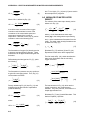
A.2 VARIANCE OF WATER VAPOR
DENSITY
Where OC1 is defined by Eq. (10).
( )
k o C oMoP
−1 ′
OC1 = L v
w′ T
−k w
R
(10)
It would be more convenient if the oxygen
correction could be written in terms of the
covariance of the vertical wind speed and
temperature instead of the inverse of
temperature. With that in mind, Eq. (6) can be
rewritten to take on the following form.
w ′ρ′ v =
(
w ′ InVh
)′
− xk w
+
ko
−k w
( w′ρ′o )
and T is in Kelvin. Eq. (14) and (15) were used in
the example SPLIT programs.
The variance of the water vapor density can be
written as in Eq. (16).
2
σρ
v
=
(12)
− xk w
− OC LE
(14)
where
OC LE = L v
The final result is Eq. (18), which describes the
water vapor fluctuations and the coinciding
oxygen correction.
( ρ′v ) 2 = ( − xk w ) −2 (InVh ) ′
A-2
(
)
(15)
2
+
2 xk o C oMoP
R
(InVh )′ ( T −1)
′
xk o C oM oP 2 −1 ′ 2
+
T
R
( )
(18)
The last two terms in Eq. (18), which are the
oxygen corrections, are cumbersome to
calculate. They can, however, be rewritten in a
simpler approximate form.
Substitute Eq. (7) into (4) and differentiate. This
leads to Equation (19) below.
ρ′v =
k o C oM oP
w′ T′
−k w RT 2
(17)
Substitute Eq. (17) and then (4) into Eq. (16).
Expand and collect terms where appropriate.
(13)
Directly substituting Eq. (13) into Eq. (11) and
multiplying by the latent heat of vaporization
yields the following.
LE = L v
(16)
and ρ′v is the instantaneous fluctuation from the
mean. The water vapor density fluctuations can
be written as in Eq. (17).
The fluctuations in pressure are very small over
a typical flux averaging period. Thus, Eq. (12)
can be written as follows:
C oMoP
ρ′o = −
T ′.
RT 2
N
( )2
= ρ′v
where ρv is the instantaneous water vapor
density, ρv is the average water vapor density,
C oM oP
C oM o
ρ′o =
T′
P′ −
RT
RT 2
)′
N
=
( )2
Σ ρ′v
ρ′v = ρv − ρv
Differentiating the ideal gas law, Eq. (7), yields
the following.
(
)2
(11)
The fluctuations of oxygen (O2) density are due
to pressure and temperature changes. These
fluctuations can be approximated using the first
derivative.
w ′ InVh
(
Σ ρv − ρv
(InVh ) ′
− xk w
−
k o C oM oP
T′
−k w RT 2
(19)
APPENDIX A. KRYPTON HYGROMETER IN WATER VAPOR MEASUREMENTS
where T is in Kelvin. Directly substitute Eq.
(19) into (16) and ignore the last term with order
T
−4
. This yields Eq. (20).
( ρ′v ) 2 =
′ 2
InVh
(
)
( − xk w ) 2
+ OC VAR
(20)
where OCVAR is defined by Eq. (21).
OC VAR
2C oM oP
= −
RT 2
ko
x −k w
(
)2
′
′
T InVh (21)
(
)
To find the standard deviation of water vapor,
simply take the square root of Eq. (20).
A-3
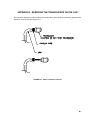
APPENDIX B. REMOVING THE TRANSDUCERS ON THE CA27
Firmly hold the transducer, while loosening the knurled knob. Once the knob is loosened, gently pull the
transducer from the arm (see Figure B-1).
FIGURE B-1. CA27 Transducer and Arm
B-1
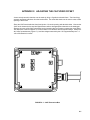
APPENDIX C. ADJUSTING THE CA27 ZERO OFFSET
A zero velocity anechoic chamber can be made by lining a 5-gallon bucket with foam. The foam lining
prevents acoustical reflections from the bucket walls. Two small dish cloths can be used to close off the
opening of the bucket.
Place the CA27 head inside the foam-lined bucket. Cover the opening with the dish cloths. Connect the
CA27 to the electronics box and the Signal/Power cable to the appropriate channels on the datalogger.
Remove the cover of the CA27 electronics box by loosening the four screws to expose the circuit board.
Use Instruction 2 with a multiplier of 1 and an offset of 0 to measure the wind speed voltage. Slowly turn
the “offset” potentiometer (Figure C-1) until the voltage measured by the 21X is approximately zero. A
±20 mV fluctuation is normal.
FIGURE C-1. CA27 Electronics Box
C-1
APPENDIX D. LIST OF VARIABLES AND CONSTANTS
ρ′v
ρa
ρo
ρv
BD
Co
Cp
CP
e
es
F
G
h
H
ko
ko1
ko2
kw
LE
Lv
LV
Ma
OCLE
OCSD
P
q
Q
R
RA
RD
RH
Rn
RV
S
SDR
T′
TA
Vh
Vo1
Vo2
W
w′
x
z
zom
g m-3
g m-3
g m-3
g m-3
kg m-3
J kg-1 K-1
J kg-1 K-1
kPa
kPa
W m-2
W m-2
m
W m-2
m3 g-1 cm-1
m3 g-1 cm-1
m3 g-1 cm-1
m3 g-1 cm-1
W m-2
J g-1
J g-1
g mol-1
W m-2
g m-3
kPa
kg kg-1
kg kg-1
J mol-1 K-1
kg m-3
kg m-3
%
W m-2
J kg-1 K-1
-2
Wm
-3
gm
C
K
mV
mV
mV
kg kg-1
m s-1
cm
m
m
Instantaneous deviation of water vapor density from mean
Density of moist air
Density of oxygen
Water vapor density
Bulk density of soil
(0.2095) fraction concentration of oxygen in the atmosphere
Heat capacity of moist air
Heat capacity of moist air
Vapor pressure
Saturation vapor pressure
Soil heat flux measured by the heat flux plates
Total soil heat flux
Height of the Atmospheric Boundary Layer
Sensible heat flux
(0.0045) Absorption coefficient for oxygen
Absorption coefficient for oxygen on line 1
Absorption coefficient for oxygen on line 2
Absorption coefficient for water vapor
Latent heat flux
Latent heat of vaporization
Latent heat of vaporization
(32) molecular weight of oxygen
Oxygen correction on latent heat flux
Oxygen correction on variance of water vapor density
Atmospheric pressure
Specific humidity
Specific humidity
(8.31) universal gas constant
Density of moist air
Density of dry air
Relative humidity
Net radiation
Gas constant for water vapor
Soil storage term
Standard deviation of water vapor density
Instantaneous deviation of air temperature from the mean
Air temperature
Signal voltage from the krypton hygrometer
Signal voltage for oxygen on line 1
Signal voltage for oxygen on line 2
Soil water content on a mass basis
Instantaneous deviation of vertical wind from the mean
Krypton hygrometer path length
Height
Roughness length for momentum
D-1
APPENDIX E. REFERENCES
Brutsaert, W.: 1982, Evaporation into the
Atmosphere, D. Reidel Publishing Co.,
Dordrecht, Holland, 300.
Buck, A. L.: 1976, “The Variable-Path LymanAlpha Hygrometer and its Operating
Characteristics," Bull. Amer. Meteorol.
Soc., 57, 1113-1118.
Campbell, G. S., and Tanner, B. D.: 1985, “A
Krypton Hygrometer for Measurement of
Atmospheric Water Vapor Concentration."
Moisture and Humidity, ISA, Research
Triangle Park, North Carolina.
Dyer, A. J. and Pruitt, W. O.: 1962, “Eddy Flux
Measurements Over a Small Irrigated
Area”, J. Applied Meteorol., 1, 471-473.
Gash, J. H. C.: 1986, “A Note on Estimating
the Effect of a Limited Fetch On
Micrometeorological Evaporation
Measurements”, Boundary-Layer Meteorol.,
35, 409-413.
Goff, J.A. and Gratch, S.: 1946, “Low-Pressure
Properties of Water from -160° to 212°F”,
Trans. Amer. Soc. Heat. Vent. Eng., 51,
125-164.
Hanks, R. J. and Ashcroft, G. L.: 1980, Applied
Soil Physics: Soil Water and Temperature
Application, Springer-Verlag, New York.
Shuttleworth, W. J.: 1992, “Evaporation”
(Chapter 4), in Maidment (ed), Handbook of
Hydrology, Mc Graw-Hill, New York, 4.14.53.
Stull, R. B.: 1988, An Introduction to Boundary
Layer Meteorology, Kluwer Academic
Publishers, Boston.
Tanner, B. D.: 1988, “Use Requirements for
Bowen Ratio and Eddy Correlation
Determination of Evapotranspiration”,
Proceedings of the 1988 Specialty
Conference of the Irrigation and Drainage
Division, ASCE, Lincoln, Nebraska, 19-21
July 1988.
Tanner, C. B.: 1979, "Temperature: Critique I",
in T. W. Tibbits and T. T. Kozolowski (ed.),
Controlled Environmental Guidelines for
Plant Research, Academic Press, New
York.
Webb, E.K., Pearman, G. I., and Leuning, R.:
1980, “Correction of Flux Measurement for
Density Effects due to Heat and Water
Vapor Transfer”, Quart. J. Roy. Meteor.
Soc., 106, 85-100.
Weiss, A.: 1977, “Algorithms for the
Calculation of Moist Air Properties on a
Hand Calculator”, Amer. Soc. Ag. Eng. 20,
1133-1136.
Lowe, P. R.: 1977, “An Approximating
Polynomial for the Computation of
Saturation Vapor Pressure”, J. Applied
Meteo., 16, 100-103.
Panofsky, H. A. and Dutton, J. A.: 1984,
Atmospheric Turbulence: Models and
Methods for Engineering Applications, John
Wiley and Sons, New York.
Schuepp, P. H., Leclerc, M. Y., MacPherson, J.
I., and Desjardins, R. L.: 1990, “Footprint
Prediction of Scalar Fluxes from Analytical
Solutions of the Diffusion Equation”,
Boundary-Layer Meteorol., 50, 355-373.
E-1
This is a blank page.
Campbell Scientific Companies
Campbell Scientific, Inc. (CSI)
815 West 1800 North
Logan, Utah 84321
UNITED STATES
www.campbellsci.com
[email protected]
Campbell Scientific Africa Pty. Ltd. (CSAf)
PO Box 2450
Somerset West 7129
SOUTH AFRICA
www.csafrica.co.za
[email protected]
Campbell Scientific Australia Pty. Ltd. (CSA)
PO Box 444
Thuringowa Central
QLD 4812 AUSTRALIA
www.campbellsci.com.au
[email protected]
Campbell Scientific do Brazil Ltda. (CSB)
Rua Luisa Crapsi Orsi, 15 Butantã
CEP: 005543-000 São Paulo SP BRAZIL
www.campbellsci.com.br
[email protected]
Campbell Scientific Canada Corp. (CSC)
11564 - 149th Street NW
Edmonton, Alberta T5M 1W7
CANADA
www.campbellsci.ca
[email protected]
Campbell Scientific Ltd. (CSL)
Campbell Park
80 Hathern Road
Shepshed, Loughborough LE12 9GX
UNITED KINGDOM
www.campbellsci.co.uk
[email protected]
Campbell Scientific Ltd. (France)
Miniparc du Verger - Bat. H
1, rue de Terre Neuve - Les Ulis
91967 COURTABOEUF CEDEX
FRANCE
www.campbellsci.fr
[email protected]
Campbell Scientific Spain, S. L.
Psg. Font 14, local 8
08013 Barcelona
SPAIN
www.campbellsci.es
[email protected]
Please visit www.campbellsci.com to obtain contact information for your local US or International representative.