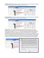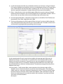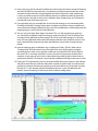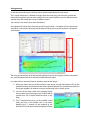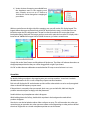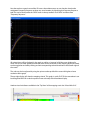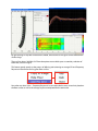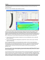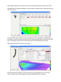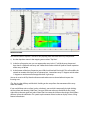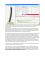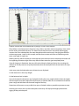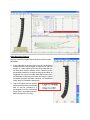
1
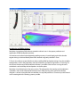
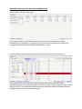
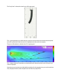
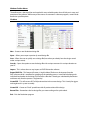
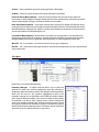
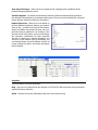
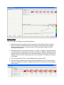
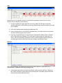
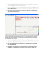
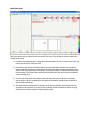
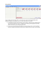
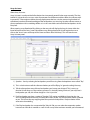
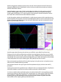
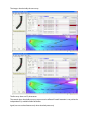
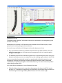
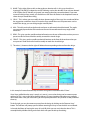
An introduction to
Introduction to EAW Resolution™
Resolution is proprietary EAW software created to aid end users in the proper prediction and
application of EAW loudspeaker products.
Its intuitive work surface and exceptional modeling accuracy is based largely on the fact that the
engine driving it is derived directly from EAW’s internal usage only software F-Chart.
F-Chart is the software responsible for not only modeling EAW loudspeaker designs but also to define
the algorithms used in the proprietary acoustic correction signal processing known as “Focusing”. For
this reason, the accuracy of the Resolution software is unrivaled as the end user is using the same
calculations used to develop the loudspeakers in the first place.
Resolution is not limited to just line array systems. The software has the capacity to also implement
subwoofers and standard trapezoidal enclosures from EAW. The long-term goal of the software
designers is to have a program that can calculate as many EAW products as is necessary to aid the end
user in creating the best sounding systems possible.
The Work Surface: Venue Tab, Array Tab and Mapping Area
The Venue tab is where the work begins.
It is the area in which you will build the room that will house your loudspeaker array design.
The default view for Resolution is a section but a plan view can also be selected to see horizontal
coverage and interaction between adjacent loudspeakers or arrays.
Once the venue has been designed the user can now click over to the Array Tab work area.
This is where you will select and place the desired loudspeakers within your room model.
You have the option of manually entering all of the necessary data, using the software’s very powerful
“Array Assistant” or use a combination of both to achieve the perfect balance of what the computer
calculates and what you see as the perfect design.
The “Array Pane” is where the virtual arrays will be presented.
This is your opportunity to visualize the arrays shape and to also review the mechanical data required
to install a system that is both accurate in its deployment and also safe in its capacity.
The power of Resolution is realized in the SPL “mapping area”.
This is where hundreds of calculations are performed by the software and the results of all your hard
work are displayed.
Not only can you view the arrays individually or combined in the mapping area, you can also see these
arrays displayed in both section and plan views for finite array adjustment.
Windows Toolbar Menus
The toolbar across the top of the work area holds many valuable options that will aid you in setup and
execution of the software. While many of the menus are common in software programs, some include
Resolution-specific options.
File Menu
New – Creates a new Resolution design file
Open – Allows you to open a previously stored design file
Save – Allows the user to quickly save a design file (best when you already have the design stored
under a unique name)
Save As – Opens the option to save the design file with a unique name and in a unique location on
your PC
Import – This is where the user may import an EASE file into the software.
Export EASE File – This feature will create a “single-balloon” file that can be imported into the
EASE software which is excellent for speeding up the modeling process. Instead of calculating each
individual loudspeaker in the design, EASE receives a file that is already pre-calculated by Resolution
and hence only needs to process a single entity!
Create PDF – This will create a PDF of all pertinent data in the current design. This is handy for riggers
and stagehands in system assembly
Create CSV – Creates an “Excel” spreadsheet with all pertinent data of the design.
Recent Files – Remembers the last design files you were working on for quick reload.
Exit – Exits the Resolution program
Edit Menu
The “Edit” menu is very small.
This is where you can Undo or Redo previous keystrokes.
Undo - If you dislike what you just did to the perfect design you can “Undo” the move.
Redo - If you decide that you liked it after-all you can redo the move again with “Redo”
View Menu
The “View” menu has many options that are extremely helpful to the operator of the software.
Aiming Lines – This will toggle on or off green lines that extend from each individual loudspeaker in
the array to the point where it impacts a surface. The aiming lines extend perpendicular to the face of
each enclosure but do not define the absolute coverage. They are a visual reference for the user to see
where each enclosure is projecting.
Aiming Coverage Lines – This will toggle on or off two red lines that define the usable upper and
lower extremities of the arrays coverage. The aiming coverage lines can be used as the upper limit
of focus in venues where back wall reflections or noise levels off-site are a concern. It represents the
soft edges of the systems coverage. If the user is required to obtain maximum throw and SPL to the
back of the venue, the green aiming line of the top enclosure of the array should be used as the top of
coverage. This will have the side-effect of some wasted energy above the coverage area and some loss
of coverage down front so take this into account when designing.
SPL – This toggles on or off the entire SPL routine in Resolution. It may seem obvious that the SPL
routine is why you are using the software to begin with but this option allows you to turn it off while
you are in the process of building both the venue and the intended arrays saving valuable RAM
energy. The number crunching that takes place in the routine can be intense!
SPL Map – Toggles on or off the SPL mapping feature. The surfaces themselves will continue to plot
the SPL for the design but the overall vertical and horizontal map will be bypassed. Again, this is a
time-saving and RAM-saving feature.
Contour Lines – In each design, it is possible to show vertical and horizontal isocontours defined in
various stages of SPL loss. These plots will overlay on the SPL map and are useful to clarify the shape of
the coverage and how well it matches the audience geometry. The contours can be viewed even when
the SPL mapping has been toggled off.
Frequency Response – Once frequency / SPL points have been defined (more on this later), the
frequency response at each location can be viewed. This feature, like all features in Resolution, works
in an anechoic environment and does not include any reflective data. Consider each of the points as
virtual measurement mics giving accurate SPL and equalization data.
Array Pane – Toggles on or off the Array Pane within the design work area (allowing more visual space
for the other two panes)
Venue Pane - Toggles on or off the Venue Pane within the design work area (allowing more visual
space for the other two panes)
Property Pane - Toggles on or off the Property Pane within the design work area (allowing more visual
space for the other two panes)
Insert Menu
The “Insert” dropdown menu provides to simple functions:
Array – This will automatically launch the Array Assistant feature within the software providing the
user with an extremely fast and accurate way of placing arrays.
Floor – This will place a new floor within the model. Be advised that this is a “new” floor and not an
addition to a currently implemented floor already placed within the model.
Options Menu
Like the View menu, the Options menu has many powerful features that enhance the experience of
using the Resolution software.
Automatically Check for Updates – By selecting this feature, Resolution will periodically check for
new, revised versions of the software when connected to the internet. The user will be prompted
when there is a newer version and you will have the option to install or not install the newer version
Temperature And Humidity – This opens up a configurable box that allows
the user to include the current temperature and humidity into the design using
EAW’s very powerful air-loss calculations. These values will vary the overall
outcome of the mapping so be certain that the values are correct.
Without Air Absorption – By default, Resolution plots its SPL mapping data with the inclusion of air
loss. This is only practical as sound is always affected by air over distance. However, if one should want
to see the difference that air loss is making on the design, the feature can be disabled by toggling it off
here.
SPL Interpolation – This allows the user to set the resolution of the SPL mapping. Three choices are
offered from fastest to best. Fastest takes less time to calculate but provides plots that are more coarse.
These are ok for rough calculations but should not be relied upon for the final design review. Normal
provides better resolution of the mapping but is still somewhat coarse. Best is the option of choice for
obtaining extremely accurate mapping. The trade-off being that it takes longer to crunch the numbers
than the other two options.
Side View Contour Lines – When the option to see contour lines has been selected, the user will have
three choices as to how these contours will be viewed in the section.
Top View Contour Lines - When the option to see contour lines has been selected, the user will have
three options as to how these contours will be viewed in the plan.
Design Factor – This is the most important feature within Resolution and every care should be
taken that it is set accurately. This feature modifies the limits of the mechanical rigging and there
are four options available (5:1, 8:1, 10:1, 12:1). The design factor that you decide to use should match
the acceptable level of safety in your particular country. In the United States, a 5:1 design factor is
generally considered to be acceptable but other countries such as Germany are much higher at 10 and
even 12:1! Using higher ratios in the design factor will limit the number of enclosures one can hang in
an array and also limit the tilt both up and down that one can achieve. The option opens a dialogue
box that reviews the safety considerations one should be aware of before altering the design factor.
SI Units – Selects the Metric option for entering all data in Resolution
US Units – Selects the Imperial option for entering all data in Resolution
Cartesian Venue Measurements – Used when measurements are based on known points of
intersection in width, height and length. Recommended when working from scale drawings and for
venues where heights of objects are known relative to one another.
Polar Venue Measurements – Used when measurements are based on height and distance of the
starting point of an object where an objects length and angle (if known) to an end point are known.
Recommended for measurements made in a venue where relative measurements are unknown but
start and end points of individual objects are.
Laser Venue Measurements – Measurements are relative to a single point in a venue defined as
a beginning and end point of an object in angle and distance from the same point of observation.
Recommended when a laser range finder and inclinometer are used together to collect data.
Max SPL – SPL is measured as a maximum loudness for any given frequency.
Flat SPL – SPL is measured as the highest loudness level where all frequencies can be sustained at the
same output level
Tools Menu
Under Tools, you will find the following:
Inventory Manager – A helpful tool that allows you to tailor the
software to match your existing equipment roster. By selecting or
deselecting from the inventory menu, the software will omit products
which you do not own. Any products highlighted in blue in the
inventory manager list are hyperlinks to the EAW website for product
pdf’s (requires internet hookup). The version number of the product
in Resolution is to the far right. Clicking on the version number will
open a box detailing “release notes” for that particular product. To add
or remove a product from Resolution, check or uncheck the circle to
the left of the Inventory Manager menu. All products remain within the
software but do not show themselves in any menus.
Auto-adjust SPL Range – Allows the user to match the SPL mapping to the capabilities of the
products being displayed on-screen.
Check For Updates – By default, the Resolution software will check automatically for updates to
the software if the computer is connected to the internet. The user can also command for a check of
recent software updates by clicking on this feature.
Keyboard Shortcuts – Allows the user to define up
to three different keyboard shortcuts per feature.
Click on the + symbol to the right of the shortcut
display and follow the prompt to insert your own
personal shortcut preferences. By clicking on the
shortcut box for each action, you may also change
the keystroke combination for that particular
shortcut or remove the shortcut altogether and
start over. At the bottom right of the display, you
can click the button “restore to defaults” to erase all
custom keyboard shortcuts and return the feature
back to original.
Help Menu
Two brief choices under the Help menu:
Help – Opens the user help files for the software as a PDF file. This file can then be easily printed out
and kept for future reference.
About – Displays the version of Resolution that you are currently running.
Building a Venue
Here are the steps to building a venue within Resolution:
1) Select the type of measurement data you are going to use to build the surfaces (Cartesian,
Polar, Laser). We have selected Cartesian for this example. Using Cartesian measurements
assumes that you have access to room drawings with accurate depth, height and width
dimensions for the venue.
2) The three data points you will need to enter are (X = Range, Z = Height, Y = Width). Enter Start
X to define where the surface begins on the first surface. Start Z will define the height from the
0 reference (lowest possible point). This can either be the floor itself or you may choose to use
the floor surfaces instead as listening levels (ears of the audience). For simplicity, we will enter
0 as the floor.
3) Now you may enter End X. This is the total depth of the first floor surface.
4) Once this has been defined you can enter the height of the floor at the rear. The angle of the
floor is now defined if the second Z is different than the first Z. If they are the same, a flat floor
will be created.
Rake
Now that we have a single floor surface, we should look at attaching a rake to it as this is fairly
common for most theaters in North America.
1) Use the + button to the right of the floor we have just built. This will drop in a rake that
attaches itself to the end of the floor you have just built but the data points will of course need
to be modified.
2) Enter in the additional data required to complete the rake.
3) Now you should enter in a name for the completed floor so as to keep track of what surfaces
are what as the design gets more involved.
4) If you are just experimenting, you may remove the rake again by clicking on the – button to
the far right of the rake dimensions. This will restore you back to the first surface that was
drawn. You can also left-click and drag the surfaces around to approximate the dimensions
you looking for and then refine them once you are happy with the basic shape.
Balconies
More than occasionally, you will find yourself needing to enter balconies in your venue. This is
accomplished in a different manner than entering a rake.
1) At the bottom right of the venue tab, you will find a button marked “Add Floor”. Clicking on
this button will drop in a generic floor to your drawing that is completely separate from the
floor and rake you have previously built.
2) The floor must be built just like the main floor. Enter in the X, Z co-ordinates for the start and
end point of the floor as defined in the room drawings.
3) You can also rough the dimensions in by clicking on points within the floor to drag it around. If
you want to remove the floor, you can click on the button in the bottom right of the Venue tab
that says “Remove Floor(s)”
4) Don’t forget to name the surface once you are happy with the results. It helps to keep track
when building complicated venues.
Front-of-House Position
If there is a free-standing FOH location within the venue, it is a good idea to position it accurately.
Resolution may modify the aiming of the system slightly to account for the FOH position when the
user decides to use “Array Assistant.”
1) Start by selecting which surface the FOH will be located on. If there is only a single surface, this
won’t be necessary but if there are balconies involved and the FOH is located on one, you can
define this now. FOH will default to the first surface.
2) Enter in the X coordinates for FOH in “Distance To FOH”. This defines how far back from the
origin the position will be.
3) Finally enter in the “Y Offset Of FOH”. It is not uncommon for FOH to be located off-center
in a venue. It is usually preferred by many engineers to locate themselves outside of the
power alley.
Width (Plan View)
Now is the time when we should switch over to the “Top View” in the design to set the Y coordinates
(width) of the venue.
1) Located in the mapping area is a drop-down box that allows the user to switch views from side
view to top view. Let’s select top view.
2) Now that we can see the venue from above, go back to the Venue tab above and to the far
right of each floor surface we have entered, you will see the cell for entering the Width of the
venue. Enter the width of each surface here. (Currently, Resolution is limited to absolute width
measurements. Fan-shaped and asymmetrically shaped rooms are not currently possible but
we are working on it.)
3) As in the side view, there are numerous click and drags that you can do to the surface if a
coarse design is all you are looking for. Absolute measurements should always be refined in
the cells of the Venue tab.
4) Also note that I have offset the FOH location. It can be seen clearly in the Plan View but will
disappear in the side view as we may not be on the axis of the FOH location. We can change
that later once we have entered some loudspeaker data.
Storing a Venue
If you are happy with the design and it is a venue that you may have to do repeatedly but with
different loudspeaker arrangements, you can save the room data as its own file.
1) In the bottom left corner of the venue tab, you can click on “Save Preset”. This will allow you to
give the venue a name and store it in a folder of your choosing. No loudspeaker data will be
stored in this file. This is for storing room data only!
2) If you want to reload the file or load a file from a previous design work, use the “Load Preset”
button to navigate to your folder of stored venues. Double-click one to open it up for editing.
Array Assistant
About Array Assistant:
Array Assistant is a tool provided in Resolution that is extremely powerful when setup correctly. The idea
behind AA is that the user sets up a series of parameters for the feature and then allows the software with
its powerful F-Chart engine to derive the array deployment that best suits the venue using hundreds of
calculations based on intimate knowledge of the loudspeakers you are using. No other software comes as
close to perfection with its modeling abilities as it is the same math used to build the loudspeakers in the
first place.
When creating a new Resolution file, clicking on the array tab will display the Array Assistant within the
lower left corner of the “array” panel. Subsequent arrays being placed with AA will require the user to
click on the “Insert” menu at the top of the screen and then select “Add Array”. This will launch a new
Array Assistant panel.
1) Speakers - Start by selecting the loudspeaker you will be using from the dropdown menu called “Top”.
2) This is also the time to tell the software whether you will be “flying” or “ground stacking” the array.
3) Tell the software how many of these loudspeakers you have at your disposal. This is not to say
that the AA will always use the number you enter. It is basically setting a limit so if you only have 8
loudspeakers per side, AA will not design for 12 or 16 per side.
4) Each loudspeaker may have a variety of “Greybox” DSP settings available to it based on the size
and / or configuration of the array. The drop down menu under “Top” will reveal the choices available
to you. This insures that any mapping done for a particular loudspeaker / Greybox choice will be
accurate in the modeling.
5) If the Top loudspeaker has a companion like 740 with 730; you can select the companion speaker
here and set a limit for its numbers as well. AA will use up to the maximum number you have entered.
6) As with the top element of the array, the bottom element may also have a variety of “Greybox”
DSP settings available to it based on the size and / or configuration of the array. The drop down
menu under “Bottom” will reveal the choices available to you. This insures that any mapping
done for a particular loudspeaker / Greybox choice will be accurate in the modeling.
7) Flybar – Normally, there is only one default choice of flybar for any given enclosure selected.
However, there are exceptions such as the KF760 which has two generations of flybars. If this is
the case, the user may select which version of the flybar they are currently using.
8) Once the appropriate flybar is selected, the “Hang Style” must be defined. For KF740 there are
three choices, Front / Rear, Single-Point, Left / Right.
9) The last set of parameters on the first panel of “Array Assistant” has the user define where the
array will be placed within the model. The user is free to define the “X” location, minimum trim
and maximum hang height before proceeding to the next page.
On the second panel of “Array Assistant”, the user defines the coverage goals of the array. By
default, the coverage is as close to zero “Z” as possible and as far out as the model has been
defined in the venue measurements. However, the user may want to define lesser amounts of
coverage in a larger venue. As an example, a theater that sells the full house on a Friday night
but only half-house for a children’s Saturday matinee? The absolute coverage of the array can be
defined on this panel.
10) Array Options - The first option allows some restriction on how the array angles will be
deployed. You can select or deselect the use of “Non-Incrementing Splays”. Some designers
adhere strictly to a spiral-array” approach of deploying line arrays. This means that the angles
between enclosures will always increase from top to bottom. Others will allow the angles of
the array to adapt themselves to match the contour of the audience. If you choose to create
spiral arrays, you would deselect
this feature.
11) Front splays may also be selected. By default, the software has this feature turned off. Opening
the fronts of EAW line array enclosures is possible but not highly recommended. Best results
are obtained when the fronts are tight together but there are occasions when audio triage
is necessary either to cover the entire audience due to an insufficient number of enclosures
on hand or to try and split an array to miss reflections from a balcony face, etc. The feature is
normally off so you will have to turn it on.
12) Coverage allows the user to modify the start and end of coverage as was mentioned earlier.
Checking the “Modify Coverage” button opens the feature and allows the user to define new
start and end of coverage conditions for the array. These modifications will be displayed on the
mapping page as a set of vertical, dashed blue bars.
13) The user may also select “Allow Upper Overshoot”. This uses the top enclosures green “onaxis” aiming line to define the top of coverage as opposed to the red “Top Of Coverage” line
normally used to define the end of coverage. This can be a desirable change as it can mean
more SPL being delivered to the back of the audience however care should be used as it also
means there could be enhanced slap back and reflections caused when using this feature
indoors.
14) Next the coverage goals are defined using a simple pair of sliders. The first slider named
“Coverage Goal” basically controls the trim height of the array. By flying the array higher
and tilting it down more, we can provide a more even coverage of the SPL front to back of
the venue. This is not always desirable as it does raise the array away from the front of the
audience. Certain types of music such as Heavy Metal may actually prefer to have the array
quite loud at the front. This feature is also limited by available trim height in the venue as well.
15) Finally, the “SPL Requirement” slider can be used to define how many enclosures the software
will pull to create the array. With the slider all the way left to “spoken word”, the software will
pull the least amount of enclosures possible to cover the audience area. If the slider is pulled
full right to “11”, the software will pull all available enclosures as you had defined on the
previous panel maximizing SPL for that particular audience configuration.
Storing an Array
As with the venue, the array(s) itself can also be stored independently from the venue.
This is useful if the there is a defined set design where the same arrays will always be used but the
venue will change from show to show. It allows the user to plot all of the arrays in a defined manner
and then drop and modify those arrays in different venues.
You must be in the “Array” tab to select this feature.
In the bottom left corner of the Array tab you will see two buttons. One button will save the current
array file to a name of your choosing and the other will open your array files to place in subsequent
venue layouts.
The Array tab now displays all of the data derived from Array Assistant. Angles, positions, placement,
etc., are all displayed and can be manually modified from this point.
Let’s take a look at some other features already at work on the design!
1) Hover your mouse over any of the surfaces in your design. You will notice that the SPL at that
particular location and the name of the surface will be displayed. This can be done anywhere in
the design regardless of whether or not you are hovering over an actual surface.
2) You can use the “Zoom” slider in the mapping display
area to zoom in on the design to get a closer look at
specific areas. This is helpful when the venue is very
large.
3) The “Y” location of the array can be modified. Useful
when you have a FOH location that is not center.
Matching the “Y” location of the mapping to the
location of FOH will reveal what the engineer will hear.
4) Various choices of mapping are available from
the dropdown menu in the mapping work
area. Currently we are set to 1/3 Octave at
1kHz but this can be changed to a mapping of
your choice.
Within a vertical bar on the right side of the mapping area, you will see the SPL display legend. This
legend defines the upper and lower limits of the SPL displayed in the map. It is also where you can
left click to open the SPL calibration tool. The tool is meant to match the SPL map to the current
loudspeaker being displayed. The images you have seen to this point had a custom SPL display with a
lower limit of 100dB and an upper limit of 133dB. No reason, just what I wanted to see.
Simply click on the “Auto” button and Resolution will do the rest. The sliders will relocate themselves to
the appropriate position but they can still be dragged left or right if you choose.
Hit “OK” to allow the auto-calibration to recalculate the SPL map or cancel to leave it as it was.
Virtual Mics
By double-clicking anywhere in the mapping area, you can drop countless “virtual mics” to obtain
detailed information on SPL as well as frequency response at those locations.
Each mic will display the SPL at the location and also will be color-coded so as to be easily recognized
when we launch the frequency response tool.
If the position is not exactly what you wanted, don’t worry, you can left-click, hold and drag the
positions around until you are happy with the placement.
Double-click on any microphone to make it disappear.
While holding down the Ctrl key, double-click anywhere in the background to make all mic
positions disappear.
Virtual mics can also be locked to either a floor surface or an array. This will move the mics when you
move the array or move the mics when you move a floor surface depending on what you have locked
the mic to? Right-click on a virtual microphone position to use this feature.
Now that we have a good sense of the SPL across the audience area, we can also take a look at the
anticipated Frequency Response at those very same locations by launching the Frequency Response
tool! This can be found under the “VIEW” menu in the top toolbar. Click “VIEW” and then select
“Frequency Response”
All mic positions will be displayed in the graph as well as an “average” of all the curves displayed in
white. The rest are color-coded to match the colors of the virtual mics in the mapping display and each
can be toggled on and off by clicking on their corresponding colored check-box at the bottom right of
the screen.
The scale can also be adjusted by using the spinner at the top left of the screen for higher or lower
resolution of the graph.
The top right display will show the mapping criteria. This graph is set for FLAT SPL but remember it can
be changed to MAX SPL under the options menu at the top of the Resolution display.
Another virtual mic feature available in the “Top View” of the mapping area is the “Virtual Mic Grid”.
By right clicking on any floor surface on the model, three choices of mic grids can be selected from
small to large.
The user first selects “Add Mic Grid” from the options menu which opens a secondary selection of
either 4x6, 6x8 or 8x10 grid.
This feature greatly speeds up the process of defining and reviewing an average SPL and Frequency
Response measurement for any given floor surface.
Now when we select “View – Frequency Response” we can take a look at every virtual mic placed on
the floor surface as well as the average response anticipated for the entire area.
Acoustics
Let’s move on to even more acoustical data by clicking on the button in the Array Tab work area
marked “Acoustics”
We will revisit the mechanical aspects of the array shortly.
There are a variety of things that can be done here to affect the outcome of the model post Array
Assistant. The first being the addition of subsequent enclosures to the array. If the loudspeaker
supports a companion enclosure such as the KF730 or KF737 in the case of KF740, we can add AB7473
adapter bar and a number of these enclosures to our already existing array. Bear in mind though that
this is a manual entry so we will have to manually correct some things once we have done this.
1) Go to the bottom of the loudspeaker selection area and use the dropdown menu to select the
AB7473 adapter bar
2) Go to the next available cell and dropdown to select KF730 – do this 3 times to put 3 x KF730’s
under our KF740 array.
You will see that the enclosures are there but they have no focus as of yet and you might have a
flashing “ALERT” icon at the bottom right of the work area. This is warning you that mechanically you
are exceeding one or more mechanical parameters. No worries right now as we will be visiting the
mechanical data in a little bit. We will also correct the focus of the 730’s once we go back to
geometric data.
Now we must select a new greybox that takes into account the alignment of KF740 to KF730. The next
group of dropdown’s allows us to change the greybox we had currently selected. We will now select a
740 / 730 combo greybox.
You will notice that it doesn’t matter from which enclosure we choose the greybox; it will change for all
enclosures in the array. This is because the feature is set to “Op Mode” lock which is probably the best
way for it to be for most applications. In certain situations, we might want to select 2 different greybox
settings within the same array. By clicking on the “Op Mode” lock / unlock button above the preset
selection area, greyboxes can be entered onto specific cabinets to be represented in the mapping.
Again, highly unlikely that we would need to do this in reality but the option is there if you need it.
Another feature in Resolution that becomes more valuable as multiple arrays are added to the design
is the “Solo” feature.
This feature allows you to single out arrays or combine arrays in the mapping to see their effect on
one another or on the listening areas. Solo is found in the bottom right of the Array Tab for any of the
arrays in the design. Next to it is the “Clear” button which turns off all soloing in the design.
The feature works in both side and top view modes.
To demonstrate the next feature we must use NTL720’s as the loudspeaker. This is because the
“Switch” selection refers to the onboard DSP selection utilized on EAW’s NT products.
Similar to the greybox selection previously discussed, the “Switch” positions for the NTL720 can be
changed to different levels of equalization so that it can be accurately demonstrated and analyzed
within the Resolution software.
Use the dropdown menu under “Switch” to select from the 4 choices of switch position on the NT
product. Like the greybox selection, it makes no difference which box you choose to change the
switch setting, all will follow suit. To select specific switch settings for specific loudspeakers, click on
the “Switch” lock / unlock button to allow individual selection.
As with the greybox selection, be careful that this is really what you want to do for a particular reason.
Even though the switch positions on the NTL only affect the HF (which is ok to mix and match to some
degree), it opens the possibility for error that may yield a Resolution map that is undesirable. Use this
feature only if absolutely necessary!
At the far upper right of the array tab work area, you will find a space called “Array Processing”.
Clicking on this area will launch Resolutions onboard virtual equalization! Here the user can virtually
equalize the arrays to fine-tune the systems response. Up to 10 different front-end equalization points
are available in this area and each can be fully configured for gain, Q/BW, and frequency. Also available
is fully configurable Hi and Lo pass filtering, gain, delay, polarity inversion and mute.
Data can be entered manually for the EQ’s by either typing or using the spinners or dropdown menus
and can also be modified with drag and drop.
Use the button located in the upper right area of the equalization display to hide or show the EQ
parameters.
Anything done within this equalization area is reflected in the map created by Resolution. Equalization
can also be disabled or reset if the user wishes to hide or start over on the EQ process.
As is the case with the other equalization options, the onboard “Virtual EQ” can be applied to specific
enclosures by clicking on the “processing” lock / unlock button. This allows the full suite of EQ options
to be available on a cabinet by cabinet basis. As stated earlier, great care should be taken when
performing this type of equalization to provide accurate results. Erroneous EQ points will create
adverse effects to the mapping yielding undesirable results.
The images show basically the same array:
The first array shows no EQ whatsoever
The second shows how badly an arrays response can be affected if careful attention is not paid to the
independent EQ’s available within Resolution.
Again, best to use these features only when absolutely necessary!
Array Geometry
Geometric Array Data
The button marked “Geometric” will take the user back to an area where he can change the physical
attributes of the design.
Remember that I had added 3 x KF730 enclosures to the bottom of the KF740 array but up to this
point, I haven’t made any changes to those enclosures.
Here are the steps to the things I did change to arrive at the design you see here.
1) First, I raised the focus of the array a little bit more towards the top of the audience. Since I had
added three more enclosures, I had more vertical coverage to play with so I wanted to get the
energy up a little higher.
2) This effectively threw off a lot of the focusing that Array Assistant accomplished so this time I have
elected to manually enter some new angles to the system including angles needed on the KF730’s.
You can now see that the mechanical warning I was getting earlier in the design process has now
disappeared. The warning was alerting me to the fact that one of the chain motors had become
“unloaded”. By manipulating the angles and overall tilt of the array, I was able to correct the problem
without doing anything drastic.
Let’s review the tools available to us in the “Geometric” work area.
1) To the left of the work area on the array tab are the parameters for the array itself. This includes
the arrays X, Y, Z coordinates, bumper hang-style, overall array tilt, maximum hang, minimum trim,
overall coverage and coverage modifier, pullback selector and Y-Axis rotation angle.
2) NAME - To the right of these cells are the enclosure selection cells. In this case, the cells are
showing KF740, AB7473 adapter bar and KF730 being used as the downfill. Since we have selected
a FB174 flybar, the KF740 cells are “greyed” out meaning that they cannot be altered. If you were
to start the design from scratch, you would have a full menu of choices in the dropdown boxes to
select what you would like to hang.
3) SPLAY – This is where you can modify the inter-element angles of the array. You can elect to follow
the suggestions made from Array Assistant but if you would like to see if improvements can be
made to the design, you can change angles manually here.
4) AIM – This tells you the tilt angle for each enclosure as referenced to level horizontal. The angles
are measured perpendicular to the enclosure face and do not reference the trap angle of the
enclosures.
5) REAR – This gives you the specific mechanical locations on the rear of the enclosure that you must
preset in order for the real-world assembly to match the virtual design
6) FRONT – This gives you the specific mechanical locations at the front of the enclosure that you
must preset in order for the real-world assembly to match the virtual design
7) The minus (-) button to the far right will delete the corresponding enclosure from the design.
In this example I have enlisted the help of a time-saving tool in Resolution called “Clone”
Once I have verified that the array is exactly as I want it, I can use the cloning tool to create an exact
replica of it. This is very useful when dealing with any L/R setup situation where the arrays perfectly
mimic each other. Once you select clone, you will be prompted with a new panel to set the position of
the array.
To the far right, you can also remove an array from the design by clicking on the “Remove Array”
button. The software will prompt you first before removing the array in case the click was accidental.
I also took the liberty of naming the arrays HL and HR which you can see in the tabs above. This is
accomplished by double-clicking on the tab which will open the title up for editing.
Mechanical Data
Now we are back to “Top View” so that we can properly place and rotate the arrays into position.
1) Use the dropdown menu in the mapping area to select “Top View”
2) In the Array Properties area, you can separate the arrays in the “Y” cell of the array placement. I
have chosen +20 feet for one array and -20 feet for the other which will yield an overall separation
of the arrays of 40 feet.
3) At the bottom of the Array Properties you will find a cell marked “Aim Angle”. This cell modifies the
azimuth or rotation of the array on its horizontal axis. I rotated one array +5 degrees and the other
-5 degrees to set the overall coverage of the left / right arrays.
You can also see in the Top View the distance each enclosure must throw before it impacts the
listening area.
(Tip- Pressing the shift key and left-click / holding on the array allows free movement of the array
within the model)
If you would like to omit a surface (such as a balcony), you can hide it temporarily by right-clicking
on the surface and selecting “Hide Floor”. Once you have seen what you would like to see, simply
right-click on the area again and select “Show Floor” to restore the surface to the design. Hiding floors
removes it from the calculation. This speeds up the amount of time it takes to display. A time-saving
feature in Resolution.
Let’s take a look at what is the most important feature of the Resolution software and that is
Mechanical Data!
To review what was mentioned earlier, we must first set the “design factor” for the mechanical data
which can be found under “options”. There will be a review of what design factor refers to and some
cautionary notes to review. Selectable from 5:1, 8:1, 10:1 and 12:1, each choice helps the software to
create mechanical data that will be acceptable in your region of the world.
In the example, I have created an array using 8:1 design factor and kind of messed it up a little to show
you what warnings are presented by the software. At the bottom right of the mapping area you will
see a box that displays the current “design factor” that you are working in which of course you can
change. You can click on this box also to open the “design factor” selection menu. To the left of that is a
box that will display a flashing icon that starts anytime there is an issue within the mechanical rigging
that should be addressed. Since it is a flashing icon, it is not displayed in this screen capture.
This design does have a flashing icon and if you look at the array in the “Array Pane” you will see that
certain mechanical points on the array have changed from green to yellow or red. These are cautions
that must be addressed before physically assembling this array.
The list of issues is also displayed to show you in particular what needs to be addressed. If you hover
over the flashing icon, the list will also be displayed.
In the instance of this example, we are dealing with mechanical stress to the rigging components,
which is the most serious warning that will be displayed. This means that we have created a design
that due to either its shape, quantity of enclosures or array tilt angle presents a scenario where the
rigging components could be damaged. We must remove one or more of the three variables so that
the array complies with the design factor we have selected.
Another scenario that I have created with my design is shown in this example.
The problem we are facing here is that when using a front / rear chain motor arrangement, I have asked
for too much upward tilt on the array. This doesn’t mean that I have over-stressed any of the rigging,
it means that I have unloaded the rear motor altogether and the entire array is hanging from the front
or downstage motor. I could, in this example, remove the rear motor and the array would hang at the
exact same angle it is right now.
Rotating the array too far forward can also create the same scenario in reverse where the rear motor will
be supporting the entire weight of the array while the front motor has gone completely loose.
Once this happens in Resolution, the array will not be able to be tilted any further. You are asking the
software to virtually create an array that practically cannot be accomplished in the real world so it stops
you there.
In the array pane, the loudspeaker arrays dimensions are displayed.
On the vertical axis is the arrays height.
On the horizontal axis its depth.
Across the bottom the dimensions are displayed including the arrays weight which includes the weight
of the bumper but not the weight of the chain motors or speaker cable. You must determine what these
pieces weigh and add them into the overall weight of the array.
Dimensions of the arrays are very useful when space is limited in either a portable or permanent setup.
Hovering your mouse over any of the data points of the array will display the weight placed on the
rigging at that particular point.
Other Resolution Features
Here are a few other helpful features that you will find within
Resolution
1) If you right-click in the Array Pane, you will see displayed
a choice of either “copy to image” or “copy to CSV”. Copy to
image is a screen capture of just the Array Pane that you
can now paste in other software such as “Word” to create
presentation material or to have on-hand to distribute to
stagehands for system assembly. Note that the stress dots
are displayed on the array even when the image is copied
to another program like Word. However, no mechanical
safety notes are included in the images.
2) Copy to CSV allows the user to copy
and paste all pertinent mechanical
data to also be provided in a
presentation or to be used during
setup. There is no mechanical stress
data included in the CSV copy.
Right-clicking in the Map Area of the software will allow the user to copy the complete color SPL map to other
software as well. This example shows the map being displayed in Microsoft “Word”. Colorful graphics are great
for presenting to a prospective client.