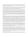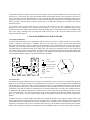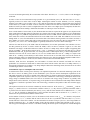
1
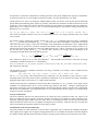
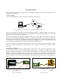
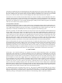
th
Source: SPIE’s 10 Annual International Symposium on Smart Structures and Materials, San Diego,
CA, USA, March 2-6, 2003.
Two-tiered wireless sensor network architecture for structural health
monitoring
Venkata A. Kottapalli*c, Anne S. Kiremidjiana, Jerome P. Lyncha, Ed Carryerb, Thomas W. Kennyb,
Kincho H. Lawa, Ying Leia
a
Department of Civil and Environmental Engineering, Stanford University
b
Department of Mechanical Engineering, Stanford University
c
Department of Electrical Engineering, Stanford University
ABSTRACT
In this paper, we make a brief study of some of the important requirements of a structural monitoring system for civil
infrastructures and explain the key issues that are faced in the design of a suitable wireless monitoring strategy. Twotiered wireless sensor network architecture is proposed as a solution to these issues and the protocol used for the
communication in this network is described. The power saving strategies at various levels, from the network
architecture, to communication protocol, to the sensor unit architecture are explained. A detailed analysis of the network
is done and the implementation of this network in a laboratory setting is described.
Keywords: Structural health monitoring, wireless sensor networks, time division multiple access (TDMA), spread
spectrum, power cycling.
1. INTRODUCTION
Extreme events like earthquakes can cause enormous damage to the health of civil infrastructures without producing any
apparent visible damage. Such damage can result in life threatening conditions evolving in the structure either in the
immediate aftermath or long after the actual event has happened. Near real-time structural monitoring of civil
infrastructure reduces the loss of human lives by warning of hazardous structures and impending collapses and also
provides information to emergency response services. In addition to extreme events, our built environment undergoes
gradual deterioration over its life span due to corrosion, fatigue, scour, etc. Thus, periodic monitoring can be used to
provide information as to the structural soundness of the civil infrastructure over its operational life.
Traditionally, structural monitoring systems were wire based, which are essentially extensions of laboratory based Data
Acquisition (DAQ) Systems. The sensors are deployed at few critical points in the structure and connected to a central
DAQ module over a cable, generally a co-axial cable. High speed Digital to Analog converters at the DAQ, convert the
analog vibration data from the input channels into a digital format and this is logged on the local data server for analysis
by the health monitoring algorithms. More recently, digital sensing units have been deployed but still are wire-connected
for data transmission to a DAQ.
For structural monitoring, the wired systems throw up a host of issues, the primary problems being those of installation
and maintenance. Laying out the cabling is expensive and time consuming. This is primarily because of the large sizes
of structures and because the points where the sensors are installed are generally hard to reach. For example, installation
time of a moderate size monitoring system can consume over 75% of the total system testing time with installation costs
approaching over 25% of the total system cost 1. In the state of California, 61 of the states 22,000 bridges have been
instrumented with costs reported to be well over $300,000 per toll bridge for a 60- channel system. A large portion of
this cost includes the laying of conduits needed to protect wires from harsh weather conditions at a cost of $10 per linear
*
[email protected]; phone 650-776-3718; The John A. Blume Earthquake Engineering Center, Stanford University; Stanford, CA
94305;
foot 2. In the event of an earthquake or other extreme events, the wired links are prone to breakage resulting in
unreliability of the data link. Also, in commercial buildings, rodent nibbling is a serious problem.
To overcome the many disadvantages of wired systems, use of wireless technologies have been proposed for structural
monitoring 1. With the advent of low cost wireless technologies like Bluetooth, IEEE 802.11 etc, there has been
considerable interest in wireless technology as a viable alternative to the wired systems.
sensor
monitoring station
wired link
wireless link
Floor View Plan
Fig. 1: Traditional Wired and Wireless sensor networks
Floor View Plan
The general approach to using the wireless links in structural monitoring has been to push the process of digitization of
the analog vibration information to the remote sensor units and then replace the wired links with wireless links to
provide data communication. Essentially, the wireless network is a STAR network, with all the sensor units
communicating with a central monitoring station. Such an approach solves most of the problems associated with wired
systems but throws up the new problems that are inherent to the wireless systems, the primary problem being that of
power. In a wired monitoring system, the remote sensor units obtain their power over the cables connected to the DAQ
module. However, in a wireless monitoring system, the remote sensor units are powered by batteries and so power is at a
premium.
Most of the research in wireless monitoring systems has focused on the development of sensor modules with embedded
computational capability and wireless communication capability provided by off the shelf radio modules like those of
Bluetooth or IEEE 802.11. These systems assume a point to point or point to multi-point communication. However,
there hasn’t been much research on developing suitable network architectures for these systems. A robust wireless
structural monitoring strategy requires the appropriate choice of the wireless network topology, the specific wireless
technology as well as a suitable protocol. In this paper we propose a wireless structural monitoring strategy for civil
infrastructures, with a focus on the system-wide sensor network. Atwo-tiered wireless network architecture with a
protocol inspired by the LEACH 3 and Bluetooth 4 protocols is proposed and designed specifically for the structural
monitoring application. The characteristics and requirements of the structural monitoring application are studied first in
order to identify the key design challenges. The two-tiered wireless network architecture is intended to handle these
issues. A communication protocol is designed and several power saving strategies in the sensor unit architecture are
considered. The proposed monitoring system is analyzed and several conclusions about the tradeoffs involved in the
system are drawn. An estimate of the maintenance cycle is made based on the power consumption of the sensor unit. A
simple implementation of the proposed network that was made in a laboratory setting is explained next along with the
experiments conducted on it.
2. THE STRUCTURAL MONITORING APPLICATION
The structural monitoring system operates primarily under two scenarios, extreme event monitoring and long term
periodic monitoring. In the event of an earthquake (extreme event), we need a near real-time performance from the
system. Information as to the soundness of the structure has to be obtained with in minutes. It is important to note that
the maximum duration of the earthquake is about 3 minutes with the majority of earthquakes lasting less than a minute.
For the long term periodic monitoring, the response of the structure to ambient loading from winds or traffic is to be
obtained. Also, as the structural properties vary with environmental conditions like temperature, humidity, or airborne
chemicals, it is necessary to obtain the structural responses under all the different environmental conditions that the
structure is subjected to over its life span. Under any given set of conditions, the duration of measurement of the ambient
vibrations is also on the order of minutes.
Civil infrastructures in general are quite large, spanning hundreds of feet and in the case of bridges may be miles long.
On account of these large sizes, the monitoring system is widespread with some of the sensors placed very remotely
from the central monitoring station. This makes the process of data acquisition difficult as wireless links have limited
range. Also, the amount of power required to transmit data over such large distances is quite large.
In a structural monitoring system, the parameters that are being measured are generally acceleration, linear displacement,
strain, angular displacements with acceleration being the most common parameter measured. Environmental variables
like temperature, humidity are also measured in order to get an accurate picture of the structural properties. Traditional
accelerometers, though high performance are very expensive, power hungry and cumbersome to deploy in structures.
With the advent of Micro Electro Mechanical System (MEMS) technology, accelerometers have become low cost as
well as low power. Peak accelerations due to ambient vibrations are in the order of hundreds of µg while a peak
earthquake acceleration would be about 2g. One key observation to be made is that, current MEMS accelerometers do
not have the dynamic range required to measure both seismic responses as well as ambient vibrations. Therefore, it
becomes necessary to use two accelerometers, one a low sensitivity accelerometer with enough range to measure
responses from extreme events and the other a low noise, high sensitivity accelerometer to perform ambient vibration
measurements.
Another important consideration is the rate at which data are generated in a sensor unit, during measurement of the
structural responses. This is important as it gives us an idea of the system throughput requirements for near real-time
performance. This data generation rate depends on the sampling rate which in turn is dependent on the fundamental
modes of vibration of the structure. For such large structures, the fundamental mode is in the order of Hertz and
therefore the sampling rates should be on the order of tens of Hertz. For a sampling rate(FS) of 50 Hz, the analog - digital
conversion resolution (b) of 16 bits, with two channels (s) of acceleration data (x and y-axes), the rate at which data are
generated per sensor unit is 1.6 Kilo bits per second (Kbps) (FS·b·s) which is not a large value. However, the overall
system contains a large number of sensor units (N) and the total rate at which data are generated in the whole system is
N· FS··b·s. For N equal to 200, the central monitoring station must be able to handle data rates of 320 Kbps under the best
case for near real-time performance, and much higher date rates depending on the sensor distribution and other overhead.
While the data generated per sensor unit are on the order of Kbps, the data that have to be handled by the overall system
are in hundreds of Kbps and could be on the order of Mega bits per second(Mbps) for larger number of sensors.
The majority of the algorithms used to analyze the vibration information are based on modal analysis procedures. For
modal analysis to be performed on a structure, it is necessary that the vibration data obtained from the different sensors
distributed in the structure be synchronized in time. The tolerance for the errors in the data synchronization is of the
order of milli seconds. In a wired system, this synchronization of the data is a trivial problem as the data from all the
sensors is being sampled at one central location. However, in a wireless environment, synchronization of data becomes a
challenge as the data are sampled at the remote sensor itself and the delay from the data sampling at the sensor unit to the
reception of the data at the monitoring station is not controlled.
As for any monitoring system, maintenance is an expensive part of the structural monitoring system. For a structural
monitoring system to make economic sense, the maintenance cycles should be long, generally years. It is safe to assume
that regular power supply is available throughout the structure to support existing infrastructure requirements like
lighting etc. However, the sensor units cannot be operated on this power as the placement of the sensors is based on the
locations of the critical structural elements and these points are generally hard to reach from the power outlets. In a wired
monitoring system, wiring has to be done at a great expense and power is the least of the problems. But in a wireless
monitoring system, the sensor units will have to depend on batteries for their power. Owing to the fact that maintenance
cycles are very long, the sensor units have to be very energy efficient if they are to survive for one complete
maintenance cycle solely on battery power.
From the above discussion, we come to some important conclusions. The system has to provide a way to synchronize the
data of the distributed sensors. For the wireless monitoring system, the system throughput requirements are on the order
of hundreds to thousands of Kbps for near real-time performance. Also, a significant number of sensor units have to send
their data over a large range. The sensor units should consume the minimum amount of power possible as they have to
survive on battery power for long maintenance cycles. Achieving large data rates and large transmission ranges require
significant amounts of power which is clearly in conflict with the requirement that the power consumption should be as
small as possible. Achieving these conflicting requirements is one important challenge in the design of the wireless
monitoring system.
A two-tiered wireless sensor network (Fig.2) is proposed as the solution to the above challenge. The system is
partitioned into two subsystems. The first subsystem consisting of a low data rate, low transmission range, energy
constrained sensor units and the other subsystem consisting of high data rate, large transmission range coordinator units
that are not energy constrained. The first subsystem forms the lower tier of the two-tiered network and the second
subsystem forms the upper tier.
3. TWO-TIER WIRELESS SENSOR NETWORK
3.1 Network architecture:
The distributed sensor units (SUs) are divided into clusters, similar to the cells in a cellular network. A local site master
(LSM) is assigned to each cluster to coordinate the SUs in its cluster and to collect the data from them during
monitoring. The clustering of sensors is done based on the proximity (in the communication sense) of the sensor units to
each other. The sensor units operate on battery power and low power operation is the primary criterion in their design.
The LSMs operate on regular wall outlet power supply, and so do not have any constraints on power. They are provided
with a battery backup in case of power failure. The clusters of SUs communicating with their corresponding LSMs forms
the lower tier and the network of LSMs forms the upper tier. The LSMs receive the data from the SUs and route the data
to the Central Site Master (CSM) over the network formed by the LSMs.
sensor
local site master
central site master
lower tier link
upper tier link
cluster
Fig. 2: Two-tier network
3.1.1 Lower Tier
The transmission range requirement of the sensor units is significantly reduced, as they have to transmit only up to the
LSM that is located within the cluster. The communication in each cluster is over the 915 MHz license-free ISM band
and the data rates are in the tens of Kbps. Also, the radio transceivers have programmable transmit power control so that
only the minimum required power is used in transmitting data. This also reduces interference between clusters. Each SU
communicates only with its LSM. The communication is spread spectrum based as it provides more reliability and also,
is mandated by the Federal Communication Commission (FCC) for all radio devices transmitting more than 0.75 mW
power in the ISM band 5. The spread spectrum used is the frequency hopping spread spectrum (FHSS). All the sensor
units in a cluster follow the same pseudo random frequency hop pattern with adjacent clusters following different
patterns.
In addition to this, the available 26 MHz wide band can be divided into chunks of fifty frequency channels each so that
adjacent clusters follow a different chunk of the 50 hop frequencies. For example, with a channel separation of 250 KHz,
the 26 MHz band can be divided into 104 frequency channels. These 104 channels can be divided into two chunks of 52
frequencies, and adjacent clusters can use a different chunk. This way, the interference between channels can be further
reduced. The 50 frequency channels per communication link is mandated by the FCC for low data rate links, specifically
when the 20 dB channel bandwidth is less than 250 KHz. The SUs in a cluster follow a TDMA schedule for
communication with the LSM. In order to maximize power savings in the SU, the lower-tier communication follows a
protocol designed with minimal handshaking.
3.1.2 Upper Tier
The LSMs in the system form the upper-tier of the network. Each LSM consists primarily of two radios and a LSM
controller. The first radio operates on the 915 MHz and is used to communicate with the SUs. The other radio operates
on the 2.4Ghz ISM band and is used to communicate with the LSMs of the adjacent clusters. The 2.4 GHz ISM band
provides more bandwidth and can support data rates in the order of Mbps. By using higher data rates for the upper-tier
network, the overall system throughput requirements are met allowing with the lower-tier network to operate on lower
data rates. The LSMs can also communicate with each other over the 915 MHz, low data rate radios and this
communication link is used for the synchronization of the local clocks of the LSMs to the global clock in the network.
Each LSM is assigned a predecessor LSM and a set of successor LSMs. Each LSM synchronizes its local clock to that of
its predecessor LSM. In this way, the whole network is synchronized to a global clock determined by the CSM.
The LSM receives the data from the sensor units over the 915 MHz band and routes it to the CSM over the upper tier
network formed by all the LSMs. Therefore, each LSM receives not only the data from the SUs in its cluster but also the
route-through traffic from the other LSMs. The communication over the 2.4 Ghz link could be based on standard
protocols like the IEEE 802.11b or on custom designed protocols. As there are no energy constraints on the LSM, it
would be easier to implement the system with a standard protocol for the upper-tier network. By allowing the lower-tier
and the upper-tier networks to operate on the 915 MHz and 2.4 GHz bands respectively, interference between the two
networks is avoided.
3.2 System components & Operation
The System is primarily composed of the Sensor Units (SUs) and the Local Site Masters (LSMs). In this subsection, we
describe their hardware architecture as well as the states in which they operate. This is essential to understanding the
hardware level power saving strategies.
3.2.1 Sensor Unit architecture
The SU consists of the SU controller, a 915 MHz radio transceiver, SRAM memory, a low sensitivity, high g
accelerometer (AccLow) like the ADXL210 6, and a sensor module containing a high sensitivity, low noise accelerometer
(AccHigh) like the Model 1221 accelerometer 10, a high resolution, low speed Analog to Digital converter and any other
sensors that might be required for improved functionality (Fig. 4). AccLow is used to measure extreme event responses
while AccHigh is used to measure ambient responses.
The SUs operate in four states Sleep, Update, Semi-awake and Awake. During the SU Sleep state, the radio transceiver
and the sensor module are in the sleep mode, drawing minimum current. The SU controller and the AccLow sensor are
power cycled to conserve power. The AccLow output is sampled by the on-chip A/D converter of the SU controller at a
low frequency of 5Hz in order to detect the onset of a possible extreme event. To perform the power cycling 6 the SU
controller powers off the AccLow sensor and sets a low frequency timer to wake up the SU controller, every 200 ms (5
Hz). It then goes into the sleep mode. When it wakes up, it powers on the AccLow and after the startup time for the
accelerometer has elapsed, it switches on the on-chip A/D converter and samples the output. Once the data are sampled,
and are found not to represent an extreme event value, it switches off the accelerometer and the A/D converter and goes
back into the low power sleep mode after resetting the wakeup timer. In this way, power cycling is used to save
significant amount of power during the sleep state of the SU. It is important to note that state refers to the state of the
complete unit, while mode refers to the state of the specific device in the unit.
In the Update state, the sensor module is in the sleep mode, the SU controller and the radio transceiver are powered on
and the AccLow is powered cycle. The SU controller is communicating with the LSM to update information in this state.
In the Semi-awake state, the radio transceiver is in the sleep mode and the sensor module, the AccLow sensor and the SU
controller are all powered on. In this state there is no transmission of data but there is active sampling of the acceleration
output. In the Awake mode, the Radio transceiver, the sensor module, the AccLow sensor as well as the SU controller are
all on. In this state, there is active sampling of the sensor outputs as well as the transmission or reception of data through
the radio transceiver.
AccLow
2.4 GHz
radio
LSM
controller
Memory
Fig. 3: Local site master
915 MHz
radio
915 MHz
radio
SU
controller
Memory
AccHigh, A/D
misc. sensors
Fig. 4: Sensor unit
3.2.2 Local Site Master architecture
The LSM consists of a 2.4 GHz radio transceiver for the upper tier communication, a 915 MHz radio transceiver for
lower tier communication, a LSM controller and memory to store the route through data (Fig.3). The LSM operates
continuously throughout the life of the network.
3.2.3 System Operation
The monitoring system’s primary function is to record the structural response during extreme events when they happen
and the ambient vibrations of the structure under different environmental conditions.
An extreme event is defined 1 to occur when the acceleration of the structure exceeds a threshold value of about 5mg.
After the onset of the extreme event, the event is defined to have ended when the acceleration remains below a threshold
value for a threshold interval of time. When the SU detects the onset of an extreme event, it enters the Active state. The
sensor unit increases the sampling rate of the accelerometer output to the required level and starts recording the data in
the SRAM memory. It notes down the time on the local clock when the onset of the event was observed. It synchronizes
with the LSM and adjusts the local clock to the LSM clock and accordingly, it modifies the event onset time that was
recorded earlier. In this way, synchronization of data, which is a key requirement of the wireless monitoring system, is
achieved. It starts alternating between the Awake state and the Semi-awake state, communicating with the LSM only at
the appropriate time slot, thus conserving power. The LSM receives the data from the SU and routes it to the CSM. Once
the event has passed and all the data has been transmitted, the SU enters the Sleep state.
For periodic monitoring, the CSM develops a schedule as to what times the ambient vibration information is to be
recorded. This schedule is developed based on the expected or existing environmental conditions. This schedule is
passed to the LSMs in the network. The SUs are generally in the sleep state and wake up a fixed number of times (w) a
day, at uniform intervals and enter the Update state. These wakeups are called the Schedule update wakeups. An SU
wakes up at these intervals, synchronizes with the LSM, and checks for any schedule updates. If it finds a monitoring
phase scheduled within the next interval, it sets a wakeup timer to wake up at the right time and goes back into the Sleep
state. The SUs wakeup at the scheduled time and enter the Awake state. After synchronization with the LSM, they
alternate between the Awake state and the Semi-active state transmitting the sampled vibration data for a predetermined
interval of time before going back in to the Sleep state. Any modifications in the schedule by the CSM and LSMs have
to be done at least one full interval ahead, if the sensor units are to identify these changes.
3.3 Lower-tier communication protocol
Within each cluster the sensor units follow a Time Division Multiple Access (TDMA) scheme for communicating with
the LSM (Fig. 5). Assuming the number of sensor units per cluster to be n, a round is defined as n+2 time slots with the
first n slots being data slots and the last two being the control slots. Each of the sensor units is allotted one specific data
slot. The first control slot is the Synch-Ack slot during which the LSM broadcasts the Synch-Ack packet. The second
control packet is called the Global-synch slot during which the LSM receives the Global-synch packet from its
predecessor in one round and sends the Global-synch packet to its successors in the next round in an alternate fashion. In
this way, global synchronization is achieved in the upper tier. Generally, each control slot is half as long as the data slot.
When the SU is sampling data during an extreme event or during a scheduled periodic monitoring phase, it transmits its
data one packet per each of its specific data slot. Also, the frequency hopping is done at the rate of one freq per slot.
Round 1
Rounds
Slots
D1
S-a
SU 2
Tx
Tx
Tx
S-a
S-a
C1
Tx
Rx
SU n
SU 1
Dn
D2
LSM
Round 2
C2
D1
Dn
Rx
Tx
S-a
Rx
Rx
D2
S-a
Rx S-a
Tx
Tx
Rx
Rx
S-a
Rx S-a
Tx
Tx
C1 C2
S-a
Rx S-a
C1: synch-ack
C2: global-synch
Di: data slot-i
S-a: Semi-active state
Active-state
Rx: Receiving
Tx: Transmitting
Time
Fig. 5: Data communication during an extreme event or periodic monitoring
The LSM does not send an acknowledge separately for each packet received from the sensor units. Rather, at the end of
the data slots of a round, the LSM broadcasts the Synch-Ack packet which contains the acknowledge bits for all the
packets received in that round as well as the previous round, incase the previous Synch-Ack packet received at the SUs
was corrupted. The Synch-Ack packet also contains the local clock information of the LSM that is used by the sensor
units to synchronize their own clocks to the LSM clock. In this way, all the sensor units are synchronized with their
LSMs during the active period of the network. The frequency hop patterns are pseudo-randomly ordered and is
predetermined by the LSM and all the SUs in a cluster are aware of the exact order. Each SU wakes up from its Semiactive state to the Awake state at the start of its data slot, transmits its data and goes into its Semi-active state for the rest
of the data slots. It wakes up on the right frequency at the start of the Synch-Ack slot to receive the packet from the LSM
before going back into the Semi-active state.
Before a sensor unit goes into the sleep state at the end of the monitoring or update phase, it informs the LSM about its
impending sleep state. Once the LSM knows that the SU is in the Sleep state, it uses the SU’s data slot for transmitting
Startup packets. The Startup packets are very small sized packets containing information about when the next Synch-Ack
packet is due. The LSM hops over multiple frequencies in the same data slot sending a packet on each hop and the
hopping is done in such a way that it covers all the frequencies in as little time as possible. In the same data slot of the
next round, based on the known frequency pattern, it listens on the right frequency for a packet from the SU. After the
SU wakes up and wants to synchronize with the LSM, it listens over a random frequency for the Startup packet from the
LSM. Once it hears the packet, it has the information about the next Synch-Ack slot and accordingly synchronizes with
the LSM. After the synchronization is done, the SU sends a control packet to the LSM in its data slot of the next round
when the LSM is listening for it. When the LSM receives this packet, it stops sending any further startup packets in this
data slot. The Startup packets are not specific for an SU and can be used by any of the SUs to synchronize with the
LSMs.
Regarding the Periodic monitoring schedules, the LSMs append these schedules to their Synch-Ack packet, so that when
the SUs wake up for schedule updating, they are able to get this information upon synchronization.
4. ANALYSIS OF THE TWO-TIERED NETWORK
4.1 Data rates versus number of sensors
Important variables in the design of the two-tiered network include the total number of sensors (N) in the system, the
number of sensors (n) that can be accommodated in each cluster, the data rates in the upper-tier (DU) and the lowertier(DL). The data rate requirements in the lower tier depend on the number of sensors in each cluster (n). The LSM has
to receive all the data generated by the n sensor units in the cluster. Therefore, DL = n·s·FS·b/α, where α is the throughput
of the link.
In order to have the best transmission range possible for a given transmit power, the data rates have to be low 5.
Typically DL has to be on the order of tens of Kbps. Assuming the number of sensor channels (s) to be 2, sampling
frequency to be 50Hz, b to be 16 and α to be 0.7, for a data rate of 10 Kbps, the number of sensors that can be supported
in each cluster (n) is found to be about 4 sensors. Therefore, smaller lower-tier data rates impose the constraint that the
number of sensors per cluster is small. As higher data rates come at the cost of higher power consumption, the data rates
should be limited to about 50 Kbps, which limits the number of sensors per cluster to about 20.
Given a fixed number of sensor units (N), the maximum data rates that are required in the upper-tier (DU) depend on the
order in which the multi-hop routing is being done. In a structure like a bridge, where the clusters are in a straight chain
along the bridge, every LSM has one predecessor LSM and one successor LSM, with the CSM located at one end of this
chain. Under this scenario, the maximum load will be on the LSM closest to the CSM. This LSM has to receive route
through traffic of (N-n) SUs and transmit N SUs worth of data to the CSM (its cluster generates n SUs data ). In short, it
has to handle (2N-n) SUs worth of data. This scenario produces the worst case upper-tier data rate requirement. DU can
be given by (1/α).(2N-n)·s·Fs·b. The throughput α is generally assumed to be 70 to 75% in the link design 5.
The best case data rate is set by the CSM. Under all circumstances, for real time performance, the CSM has to receive
the data generated by all the N sensors. Unlike the LSMs, it does not have to transmit it again as it is the final
destination. The latest 2.4 GHz radio transceivers achieve bit rates of 1 Mbps easily and are capable of supporting data
rates up to 10Mbps 5. From the above analysis DU/DL = 2N/n –1, assuming DU to be the worst case data rate. DU is about
hundred times that of DL in general and also, N is much greater than n which implies that DU is almost independent of n.
Therefore, The worst case DU can be written as (1/α)·2N·s·Fs·b without much error. For DU = 1Mbps, N is equal to 220
while for DU = 10 Mbps, it scales linearly to 2200 sensors. The best case DU is twice that of the worst case DU and can be
achieved when the clusters are distributed such that the CSM can receive data from multiple independent LSMs. This is
possible in buildings structures. In this case, the number of sensors that can be handled doubles.
Therefore, under the above assumptions, the total number of sensors that the network can handle for real time
performance is a maximum of about 2000 to 4000 sensors under current wireless data rates of 10 Mbps. However, if
non-real time performance is acceptable, or by using multiple CSMs at the monitoring station, the network can be scaled
to handle larger number of sensor units.
4.2 Estimation of power consumption and network life
As studied in the earlier sections, power efficiency is an important requirement of a structural monitoring system as the
SUs have to survive on battery power for one maintenance cycle. First, the current consumption requirements of the
individual components of the SU are studied in the different states of operation and then the duration for which these
components operate in the respective states over a year is used to estimate the overall energy consumption. Based on the
energy ratings of standard batteries, the life of the SU is estimated. The energy rating of batteries is generally milli
Ampere hours (mAh). Therefore, we represent energy as the product of current consumed in milli Amps and the duration
for which it is consumed is specified in hours. The actual energy consumed is the product of this value with the supply
voltage.
The important currents are the currents consumed by the RF transceiver in the receive (Irf_rx), transmit(Irf_tx) and the
sleep(Irf_sleep) modes. The AccLow accelerometer consumes current (Iacc_low) only when it is powered on and none when it
is powered off. The current consumed by the memory, AccHigh and the sensor module can be clubbed into Imisc_sleep and
Imisc_awake. The SU controller is implemented by a micro controller unit (MCU) and its currents are Imcu_sleep and Imcu_awake.
All the times are specified in hours and the currents in mA.
Let the number of sensors per cluster (n) be 10, the duration of each extreme event, Textreme , be 3 minutes, each periodic
monitoring phase, Tperiodic ,3 minutes and the time it takes for the SU to synchronize with the LSM, Tstartup, to be 4
seconds which is a conservative estimate. Let the total number of extreme events per year e be 5, the average number of
periodic recording per day, r, be 2 and the number of times the SUs wakeup to update their schedule per day, w, be 12.
The sleep power consumption of the SU is calculated assuming that the this power consumption is constant throughout
the operation, even when the components are actually powered on. This greatly simplifies the sleep power calculations.
As the sleep currents are very low compared to the active currents, the errors introduced are very small.
The RF transceiver is active only during the schedule update periods, the extreme event and the periodic monitoring
periods. During the monitoring phase (extreme or periodic), each transceiver transmits in its data slot and receives in one
control slot. As the control slot is half the duration of the data slot, the duration for which the transceiver transmits is
approximately 1/(n+1) and for receive is 0.5/(n+1) of the total monitoring time. The amount of energy consumed by the
RF transceiver Erf is given by:
E rf = I rf _ sleep ⋅ 8760 + I rf _ rx ⋅ T startup ⋅ (365 ⋅ r + 365 ⋅ w + e ) +
1
( 0 .5 ⋅ I rf _ rx + I rf _ tx ) ⋅ (T extreme .e + T periodic ⋅ 365 ⋅ r )
n +1
where 8760 is the number of hours in one year. For a BlueChip transceiver 7, the energy consumed in one year is found
to be 275 mAh.
The amount of energy consumed by the MCU and the AccLow (Emcu_acc) is composed of the active energy consumption
(Emcu_acc_active) and the sleep consumption (Emcu_acc_sleep). The sleep state current consumption is expressed as an average
value due to the power cycling 6 in this state. The output of the ADXL202/210 accelerometers can be sampled about
1.6ms after they are powered on, and most on-chip micro-controller A/Ds can acquire the reading in about 25 µs.
Therefore the time taken by the MCU to acquire one sample from the AccLow after it is powered on (Tacq) is about 1.625
ms. And the power cycling period (Tpow_cyc) is 200 ms (5Hz). Therefore, the average current consumption of the
Accelerometer and the MCU in the sleep mode is given by:
Tacq
Tacq
I mcu _ acc _ sleep =
( I acc _ low + I mcu _ awake ) + (1 −
) I mcu _ sleep
T pow _ cyc
T pow _ cyc
and is found to be about 26 µA for a PIC microchip MCU 11 and an ADXL210 accelerometer. From this, the energy
consumption of the MCU and the AccLow is calculated as:
Emcu_ acc = 8760⋅ I mcu_ acc _ sleep + (365⋅ r ⋅ T periodic + e ⋅ Textreme) ⋅ ( I mcu_ awake + I acc _ low ) + (365⋅ w ⋅ Tstartup ⋅ I mcu_ awake)
and is found to be 300 mAh.
The miscellaneous energy consumption, defined as the energy consumed by the memory, sensor module and other
components, is given by:
E misc = 8760 ⋅ I misc _ sleep + ( 365 ⋅ r ⋅ T periodic + e ⋅ T extreme + 365 ⋅ w ⋅ T startup ) ⋅ I misc _ awake
The Imisc_awake is an average value obtained from these components over their duration of sleep and active cycles.
Assuming that the total sleep current of these miscellaneous components is 20 µA and the total current consumption
during the awake mode is 20 mA, the Emisc is equal to about 1000 mAh.
The total sensor unit power consumption is the sum of the three components, Erf , Emcu_acc and Emisc and is equal to about
1600mAh. For an alkaline battery of size AA, the general energy rating is 2500 mAh 12. Therefore, assuming that the
sensor unit is powered by a pair of AA alkaline batteries, the life of the network is about 18 months. This is much higher
than the one year maintenance cycle requirement and so we can conclude that the network design is very robust from the
perspective of power consumption.
4.3 Cost considerations
The micro-controllers and lower tier radio transceivers are cheap and can be procured for under 15$. However, the
upper tier 2.4Ghz chip sets are expensive. Therefore, from the cost perspective, the number of clusters should be as few
as possible, implying a larger number of SUs per cluster. However, increasing the number of sensors per unit would also
require the data rates in the lower tier to be higher, lowering their power efficiency. Therefore, there is a cost factor also
involved in choosing the appropriate number of sensor units per cluster.
4.4 Limitations of the network architecture
The primary drawback of this architecture is the fact that it is applicable only in structures like buildings and bridges
where regular power supplies exist to support existing infrastructure. It is not suitable for structures where this might not
be available. Another drawback is that the local site masters are single points of failure for the sensor units in its cluster.
5. IMPLEMENTATION
The proposed two-tiered network was implemented in a laboratory environment and an experiment conducted to verify
the functionality of the system.
5.1 Network design
The network consisting of two clusters is designed. The topology is shown in Fig.8.
cluster A
cluster B
central site master
Fig. 8: Experimental setup for the laboratory prototype of the two-tier network
The lower-tier network was designed with the following design parameters. A sampling frequency(FS) of 80 Hz, the
number of sensor channels per sensor unit (s) being one channel and the number of bits per sample (b) of 16 bits. The
number of sensor units per cluster (n) should be 5.
With the above parameters, the total data generated per sensor unit is about 1.3 Kbps. For the number of sensors per
cluster to be 5, each TDMA round should accommodate 5 data slots and 2 control slots. Each control slot is half as long
as that of a data slot. Therefore the total number of time slots can be considered to be 6 slots each of duration of the data
slot. Therefore, for near real-time communication, assuming the throughput to be 75%, the required data rate in the
lower tier is about 10.4 Kbps. Therefore we use a data rate of 10 Kbps for the lower tier.
For the two clusters, the required data rates in the upper tier are just about 30 or 40 Kbps. However, the upper tier with a
data link of 2 Mbps is implemented so that the network can be scaled to a larger number of clusters in future
experiments.
5.2. Hardware & Software
The Sensor unit was implemented with a EVK915 module 8 interfaced with a sensor board developed in the lab 9 (Fig.
10). The EVK915 module contains a 915MHz BlueChip radio transceiver 7 operating at 20 Kbps baud rate. With
Manchester encoding of the data, the data rate is 10 Kbps. The actual transceiver can be setup to operate at baud rates
ranging from 2.4 Kbps to 100 Kbps. The transceiver is very low power with receiver current of 12 mA and transmit
current of 50 mA at its peak transmit power of 10 dBm. The PIC microchip microcontroller on the EVK module is used
as the SU controller. The accelerometer used is the ADXL210 and is present on the sensor board. No external memory is
used.
RangeLAN2 radio modem
BlueChip transceiver module
Atmel Microcontroller
PIC Microchip MCU
Fig. 9: Local Site Master
ADXL210
Fig. 10: Sensor Unit
The LSM was implemented with a Proxim RangeLAN2 radio modem interfaced to a EVK915 radio module (Fig 9). The
PIC microchip micro-controller acts as the LSM controller. The RangeLAN2 radio modem operates on the 2.4 GHz ISM
and with a 2 Mbps bit rate. The protocol used by the radio modem is the IEEE802.11b . It does not use any external
memory. The Central site master consists of a Proxim RangeLAN2 radio modem interfaced with a computer.
The software for the SU controller and the LSM controller was written in assembly code and embedded in the microcontrollers. The local clock is a soft clock based on a 16 bit timer and this is used for synchronization. The resolution of
synchronization depends on the data rate. For a baud rate of 20 Kbps, the synchronization obtained is ± 50 µs. The FHSS
hop patterns were obtained from a Linear Feedback Shift Register (LFSR) procedure and the hop pattern was embedded
in the code. The software for the CSM was written in ‘C’.
5.3 Experimental verification
The network consisting of two clusters was setup as shown in Fig 8. The number of Sensor Units per cluster used is two.
The data that are transmitted by the SUs in cluster B is received by the LSM-B and routed to the LSM-A which routes it
to the CSM and that transmitted by the SUs in the cluster A are transmitted by the LSM-A directly to the CSM. Two
experiments are conducted, to demonstrate the two scenarios of operation of the monitoring system.
In the first experiment, the CSM, LSMs, and the SUs are all powered on. The SUs synchronize with the LSMs and wait
for the LSM to send a trigger packet in its Synch-Ack slot. At the CSM a predetermined code is entered into the
computer which is transmitted to LSM-A. The LSM-A passes this code to the LSM-B. The LSMs broadcast the trigger
packet and the SUs on receipt of this packet start sampling the data from the accelerometer and transmit the data to the
LSMs. The CSM receives the routed data from LSM-A and prints it out on to the screen as well as stores it in a file.
When the sensor board is shaken, the accelerometer output is found to vary according to the input vibrations. After a
predetermined number of samples have been taken, the SUs stop sampling and wait for another trigger pulse from the
LSMs. This experiment is representative of the periodic monitoring scenario of the actual monitoring system.
In the second experiment, the system is powered on and the SUs are initially idle and do not listen for any packets from
the LSM. When the sensor board is shaken, the SUs start recording the data from the time the acceleration exceeded a
predetermined threshold value and simultaneously power their radios on. They synchronize with the LSMs and start
transmitting the data that are received at the CSM. The data received is found to vary according to the input disturbance.
After a predetermined number of sequential samples are found to be less than the threshold value of acceleration, the
SUs stop transmitting data and turn their radios off. This experiment is representative of the Extreme event scenario.
6. CONCLUSION
In this paper, a novel network architecture was proposed for wireless structural monitoring systems. The important
characteristics and requirements of a structural monitoring system were studied. We concluded that one of the most
important criterion for the remote sensors was power efficiency as they operate on battery power. Based on the required
sampling frequencies and the number of sensor channels on board the sensor unit, the rate of data generation per sensor
unit was found to be on the order of Kbps. However, for a monitoring system of a reasonable size, this translates to
system throughput of the order of hundred or thousands of Kbps for near real-time operation. For the sensor units to
support such data rates and transmit over the large distances that the structure spans, requires larger power consumption.
To achieve the objective of power efficiency, the network is partitioned into two tiers. The lower tier is formed by
clusters of sensor units operating on battery power and at data rates on the order of tens of Kbps in the 915 MHz ISM
band and the upper tier formed by local site masters operating on regular wall power supply with a battery backup and at
data rates of the order of Mbps in the 2.4 Ghz ISM band. The sensor units transmit their data to their respective local site
masters and the local site masters route these data to the central monitoring station.
A communication protocol is designed for the lower tier. The protocol is TDMA based and helps the SUs conserve
power by requiring them to operate their radios only when transmitting data or receiving the synchronization pulses
without having to listen idly to potential traffic. A detailed analysis of the architecture is made and the implementation of
a laboratory prototype of the proposed network architecture is described along with the experiments conducted.
To address the issue of the single point of failure of the LSM, our future work will involve incorporating selfreconfiguration capability in the sensor units. Also, our future work will include the development of a more robust
sensor unit and local site masters as wells as the actual validation through shake table tests and field tests.
ACKNOWLEDGEMENTS
This research is funded by a National Science Foundation Grant CMS-0121842. Their support is gratefully
acknowledged.
REFERENCES
1.
E. G. Straser and A. S. Kiremidjian, A modular, wireless damage monitoring system for structures, Report No. 128, John A.
Blume Earthquake Engineering Center, Department of Civil and Environmental Engineering, Stanford University, Stanford, CA,
1998.
2. Hipley, P., “Caltran’s Current State-of-Practice”, Proceedings of the Instrumental Systems for Diagnostics of Seismic Response
of Bridges and Dams, Consortium of Organizations for Strong-Motion Observation Systems, 2001.
3. Wendi Rabiner Heinzelman, Anantha Chandrakasan, and Hari Balakrishnan, “Energy-efficient communication protocols for
wireless microsensor networks,” Proceedings of the Hawaii International Conference on Systems Sciences, Jan. 2000.
4. Bluetooth SIG Inc., Specification of the Bluetooth system: Core, http: //www.bluetooth.org , 2001.
5. Jim Zyren and Al Petrick, Tutorial on Basic Link Budget Analysis, Application note, AN9804.1, Intersil Corporation, Irvine, CA,
June 1998.
6. Analog Devices, Inc, ADXL202/ADXL210: Low Cost ±2 g/±10 g Dual Axis iMEMS Accelerometers with Digital Output Data
Sheet, Analog Devices, Inc., Norwood, MA 1999.
7. BlueChip Communication AS, BCC918 UHF transceiver reference manual, BlueChip Communication AS, Oslo, Norway, 2001.
8. BlueChip Communication AS, User manual for evaluation units 915 MHz, BlueChip Communication AS, Oslo, Norway, 2001.
9. J. P. Lynch, K. H. Law, A. S. Kiremidjian, T. W. Kenny, E. Carryer and A. Partridge, “The Design of a Wireless Sensing Unit
for Structural Health Monitoring”, Proceedings of the 3rd International Workshop on Structural Health Monitoring, Stanford,
CA, USA, September 12-14, 2001.
10. Silicon Designs, Inc., Model 1221 Low noise seismic accelerometer Data sheet, Silicon Designs, Inc., Issaquah, WA, 2002.
11. Microchip Technology, Inc., PIC microchip PIC16F73/4/6/7 Datasheet, Microchip Technology Inc., Chandler, Arizona, 2002.
12. Matsushita Electric Industrial Co., Ltd, Panasonic Industrial alkaline batteries technical specifications 2002/2003, Matsushita
Electric Industrial Co., Ltd, Osaka, Japan, 2002.