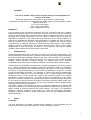
1
Durham Research Online Deposited in DRO: 02 June 2008 Version of attached le: Accepted Version Peer-review status of attached le: Peer-reviewed Citation for published item: Pechey, J. and Taylor, P. and Dixon, R. and Lawson, M. and Dinning, A. (2004) 'The role of medium voltage electrical system design in risk management for oshore wind farms.', Wind engineering., 28 (5). pp. 489-502. Further information on publisher's website: http://dx.doi.org/10.1260/0309524043028154 Publisher's copyright statement: Additional information: Use policy The full-text may be used and/or reproduced, and given to third parties in any format or medium, without prior permission or charge, for personal research or study, educational, or not-for-prot purposes provided that: • a full bibliographic reference is made to the original source • a link is made to the metadata record in DRO • the full-text is not changed in any way The full-text must not be sold in any format or medium without the formal permission of the copyright holders. Please consult the full DRO policy for further details. Durham University Library, Stockton Road, Durham DH1 3LY, United Kingdom Tel : +44 (0)191 334 3042 | Fax : +44 (0)191 334 2971 http://dro-test.dur.ac.uk 41006S326 The role of medium voltage electrical system design in risk management for offshore wind farms Jim Pechey, Philip Taylor, Richard Dixon, Mark Lawson, Andrew Dinning Econnect Ltd, Energy House, 19 Haugh Lane Ind. Estate, Hexham, Northumberland, United Kingdom NE46 3PU Tel: +44 (0) 1434 613600 Fax: +44 (0) 1434 609080 Email: [email protected]. ABSTRACT In the short-term future, UK offshore wind-farms are to be connected to the grid by Medium Voltage (MV) electrical systems. This connection is required not only for export of power but also to provide essential power supplies to critical equipment within the wind-farm. There are perceived risks to these connections, which can result in significant loss of revenue and deterioration of equipment. This paper presents the findings of a DTI funded programme of research into available MV equipment and configurations, to establish the risks of failure to these MV systems and to provide a practical guide for selecting the optimum system configuration for a particular application. Offshore access relies greatly on the prevailing weather conditions. Therefore the critical factor determining the degree of MV system sophistication is often the degree of exposure of the wind-farm to inclement weather conditions and the distance from the wind-farm to the shore. 1 INTRODUCTION Offshore wind generation is still in its infancy and is set to grow over the next decade [1]. The environmental and mechanical risks to offshore projects are reasonably well documented [2] but there has been little published material on the risks, costs of losses or loss of revenue following a failure of the main electrical connections. As a result there are no readily available standard, proven electrical connection designs for offshore wind farms. Therefore considerable risk to the security of offshore wind-farms, from these system failures, remains. Onshore wind farm developers have adopted a low capital cost approach to their MV systems [3,4]. Cabling, switchgear and protection systems are designed to simplify the installation through minimising the amount of installed equipment and most (if not all), of the wind farm MV system is disconnected following a fault and the possibilities for automatic or remote manual reconfiguration are limited. This approach for onshore wind farms is justified firstly because of the confidence built up over decades of use of readily available and reliable components used for other onshore MV systems, and secondly because of the relative accessibility of onshore wind-farms. The safety and financial implications of MV system failures in an offshore wind farm, are however some orders of magnitude greater than those for an onshore wind farm because the offshore environment presents greater safety risks, places increased restrictions of access to the farm and complicates even the simplest repair, compared with the onshore environment. This paper considers the benefits and costs of designing safeguards into offshore MV systems to sustain as much output as possible following an MV system failure, and provides a generic method for selecting optimum MV system designs. The study is for generalised situations. Particular situations would require us to check our assumptions, particularly regarding the effect of weather on access to equipment, which will vary considerably between offshore windfarms. 2 RISKS 2.1 General The work described in this paper considers three categories of risk associated with the operation and maintenance of MV systems for offshore wind farms, namely: 1 • Risks to personnel • Risks associated with the impact of security of supply to the wind turbines, and • Risk to the project economics. Personnel risks are associated with the transfer of staff between the shore and the wind farm, and between wind-turbine and offshore substation structures. Personnel are required to visit the wind-farm to repair any fault and different network designs also require differing numbers of post fault visits to reconfigure the network. The more visits to site and the more transfers that are required between service craft and offshore structures, the higher the risks to personnel. On this basis, those MV system designs, which require local manual reconfiguration, expose personnel to higher risks than designs that can be reconfigured from a remote point. There are two main risks associated with the impact of security of supply to wind turbines. Firstly, those associated with potential damage to turbines left without auxiliary power for a prolonged period of time. Examples of these include damage due to condensation, gearbox damage if the turbine has not rotated for a considerable time and prolonged re-start procedures, if the turbine controller has been without power for a significant period. The second main risk is that losing power to a wind turbine could cause failure of aviation warning lights, and also navigation lights in the case of an offshore turbine. Any offshore MV system failure can cause loss of generated output, or deterioration of equipment, both leading to loss of revenue. As an indication of the scale of the risk of investments in offshore wind-farms, we estimate that: A typical 30 turbine offshore wind farm costs about €140 million to build; The MV electrical system costs range from around €9.8 to €12.5 million; Inadequately designed MV systems can lead to losses in revenue due to electrical failures of as much as €7 million in the lifetime of the project. Consequently, the designs applied to onshore wind farms are not necessarily appropriate to offshore wind farms and the selection of appropriate MV designs for offshore wind-farms becomes extremely important at the planning stage because of their significant influence on the economics of an offshore project. 2.2 Approach to risk reduction Econnect Ltd, as part of a DTI funded project, have been carrying out research into improved and innovative MV networks for offshore wind farms, focussing on: 3 Developing network configurations and switching arrangements to minimise the loss of turbine availability following a fault and thus maximising the post fault output of offshore wind-farms Selecting the more appropriate configurations for detailed examination Establishing modes of component failure and failure rates Researching methods of failure detection and fault location Establishing a method of comparing MV system designs MV SYSTEM DESIGNS-POTENTIAL FOR MINIMIZING RISK 3.1 Alternative configurations Econnect based their research on 5 different MV system configurations developed as possible arrangements for two wind-farm construction projects, which were then in the preliminary design stage. Onshore wind farm MV systems have usually been designed using radial network configurations, Figure 1, and these may be suitable for some offshore wind farms where easy access can be assured. In this arrangement the turbines are connected to form radial circuits and, in the event of a cable failure, all turbines connected to the faulty circuit are disconnected by opening the circuit breaker protecting the faulty circuit. The radial circuit can be partly restored by disconnecting the faulted cable, thus isolating all the turbines beyond the fault and then re-energising the circuit. The turbines beyond the fault will only be restored to supply 2 once the cable has been repaired and in the meantime, they produce no power. Should it not be possible to repair the cable within a reasonably short length of time, as a result of adverse weather for example, then the consequential impact on wind farm revenues could be severe, either directly as a loss of the MV connection, or subsequently from deterioration of equipment through loss of MV supplies to the isolated turbines. The risk of equipment deterioration with radial network designs could be reduced by installing diesel generators on selected turbine platforms to provide an alternative power supply to the auxiliaries of isolated turbines. The choice is between having small standby generators to provide power for individual turbines or large standby generators to provide power to all the turbines in an isolated portion of a radial leg. It is important to note that the rating of the large generator is not determined merely by the number of turbines it has to supply but also by the cable charging duty it has to fulfill, which can be significant. An alternative configuration is to use a looped network with normally open points, Figure 2. In this arrangement, extra sections of cable are used to interconnect the radial circuits so each turbine has two routes to export power. If a single array cable failure or fault (or a single shore cable fault on a multiple shore cable installation) occurs anywhere on the looped network, every turbine has at least one remaining connected route. As soon as the faulty cable section has been isolated and the appropriate normally open point is closed, all the turbines can be restored to supply,. The output of all the turbines can now be harvested. Although the output of some of the turbines may be limited in the post-fault arrangement by cable ratings, the looped network will always deliver more energy under post fault conditions, than a radial network. The obvious way to improve further on the benefits described for the looped configuration, is to adopt a design which allows remote manual or automatic reconfiguration of the MV system, following a cable fault, by installing suitable switching equipment. 3.2 Methods of Switching We have seen that with a looped network, all the turbines can be restored to supply and earning revenue, once a faulted cable section has been isolated and the MV system has been re-energised. The requirement for relatively rapid isolation and re-energising for offshore MV systems, in turn requires these actions either to be manually controlled, from a remote position, or alternatively automatically controlled. It is therefore important to consider the balance between the value of energy lost, as a result of faults, and the cost and increased risk arising from the installation of sophisticated equipment to achieve remote rapid reconfiguration. Figure 3 shows the electrical diagram of connections to a typical onshore wind turbine, Figure 4 is a photograph of such an arrangement. The switchgear installation is minimal and the physical arrangement is shown in Fig 4. A single circuit breaker protects the turbine transformer and no additional switches or circuit breakers are used to protect or isolate faulty MV interconnections. In order to isolate a faulty cable, the entire MV system needs to be isolated, the separable “T” connectors are then unbolted at each end of the faulted cable and the MV system is re-energised. An initial visit has to be made to the wind-farm location to open the “T” connectors and a further visit to close the “T” connectors once the faulty cable has been repaired. We call this manual reconfiguration. The introduction of switchgear to the turbine connections as shown diagrammatically in Figure 5 and physically in Figure 6 allows the turbine to be switched remotely and consequently this arrangement is more appropriate for offshore than for onshore wind-farm connections. The main change to the “T” connector scheme is that each array cable is now terminated at a switch and the faulty cable can be isolated by simply operating the switch at each end of the faulted cable. This operation is obviously much faster than unbolting a separable “T” connector and the speed of isolation and reconfiguration can be faster again by remote operation of the switches. We call this remote configuration. In order to take advantage of the remote control feature of the switchgear arrangement, shown in Figure 5, it is necessary to install the correct protection and control equipment. 3 There are many cable fault locating methods available [5], it would be possible to detect the position of the fault using cable fault locators built into the protection relays at the onshore substation but a simpler and perhaps, a more reliable arrangement would be to install fault passage indicators (FPIs) on each cable feeder [6]. An FPI detects the passage of fault current and would send an alarm to the Supervisory Control and Data Acquisition (SCADA) system. Figure 2 shows the position of the FPIs on a looped network. In the event of a fault, all the FPIs between the shore and the fault will operate, whilst those beyond the fault will not operate, thus identifying the faulted cable section. SCADA signals can be carried over optical fibre cables embedded within the MV system power cables. The MV power cables however could themselves fail, therefore a fault tolerant SCADA system should be provided by means of a second path for communications, with communication route switching. We call the full use of such technology automatic configuration. 3.3 Selected configurations for examination Combining the network topologies with the different methods of switching and supply described above, gave 5 different possible wind farm designs, as follows: 1. Radial configuration 2. Radial configuration with diesel back up 3. Looped configuration with manual reconfiguration 4. Looped configuration with remote reconfiguration 5. Looped configuration with automatic reconfiguration 4 COMPONENT AND MV SYSTEM FAILURES Failure rates were derived from individual component failure rates and Mean Times Between Failure [7]. The likely failure rates for MV systems, when derived from plant and equipment failure statistics [8,9,10], depend on the MV system configurations proposed. Econnect based their calculations on the 5 configurations identified above, which were considered for a typical 30-turbine wind-farm, to give the MV system failure rates in table 1. None of these failure rates is considered to change according to the seasonal weather conditions at an offshore site. Component Number of Failures in 20 year life of Wind Farm Radial Network Looped Network Array Cable 3.09 3.35 Shore Link Cable 3.12 3.12 MV Switchgear 0.24 0.74 Turbine Transformers 3.00 3.00 Terminations 2.98 2.98 Table 1 Failures of alternative MV system configurations 5 METHODOLOGY FOR COMPARISON OF MV SYSTEMS 5.1 General A methodology was developed for comparing MV system configurations on the basis of lifetime costs. In this analysis, lifetime costs were deemed to comprise costs for 4 • MV systems as installed, complete • Lost generation over the life of the wind-farm: • Reconfiguration and fault finding over the life of the wind-farm • Repair over the life of the wind-farm The latter three costs were based on the expected number of failures in a 20-year life, as shown in Table 1 The installed costs were based on current prices for plant, equipment and installation work. The costs of lost generation were obtained by assessing the overall downtimes affecting portions of the MV systems following faults, calculating the number of generators affected and the resulting total outage times and then costing the resulting lost revenue. The downtime includes time for: • Reconfiguration • Fault finding • Repair None of these times considers statistical variation due to weather conditions, e.g. for access. Finally costs were included for labour and equipment to locate and repair faults. Lost Revenue For any given fault condition, there are two distinct phases in the post-fault period, both of which contribute to the total amount of lost generation. The first, re-configuration, phase is relatively short, but the number of unavailable turbines during this phase can be large. The second, repair phase, is usually longer, but it is likely that portions of the wind-farm generation have been brought back on line by reconfiguration and are available for generation during this phase. All wind farm MV systems are designed with appropriate electrical protection and isolation systems. The purpose of these primary systems is to isolate electrical faults quickly, in order to minimise damage to the electrical system and other elements of the wind farm [11,12]. Their secondary function however, is to minimise the amount of generation output that is ‘lost’ or unavailable, following a fault and pending a repair. This is achieved by integrating the protection and isolation systems into an overall control system. For the owner of the wind farm, lost generation corresponds to lost revenue, lost revenue being calculated using the current Renewables Obligation Certificate (ROC) value and the value of lost energy [13], both expressed in this work in terms of £ per MWh. The amount of lost generation, in the event of an MV system failure, depends on the complexity (and hence cost) of the cable array between turbines, the shore link cable system, together with the protection, isolation and control schemes. The capital costs of different designs can be combined with costs of lost generation to form a practical basis for comparing wind farm MV system designs. Put simply, lost generation (expressed in MWh) is the product of three factors: • The average energy production per turbine (MWh/hour) • The number of turbines that are unavailable • The period over which the turbines are unavailable (hours) The average energy production per turbine can be considered as a fixed parameter. It is a function of the turbine capacity, the turbine power curve and the wind regime at the site. The uncertainty of the wind 5 regime at the site can be removed from the equation if the average energy production is expressed as the turbine capacity factor for that particular site and if all turbines are assumed to have the same power characteristics, then the turbine capacity factor is a constant for a particular site and a particular design of turbine. The other two factors are heavily influenced by the design of the wind farm MV system as they are specific to the type and location of the fault under consideration and hence greatly influence the value of lost generation. 5.3 Loss of turbine availability-categories of MV system failure There are three main categories of faults, causing system failure, that require consideration when evaluating MV system designs for offshore wind farms: • Sea to shore cable fault • Inter-turbine array cable or turbine connection fault, which, because of the similar effect of other associated equipment faults, includes turbine HV switchgear, HV isolator, or cable connection fault • Turbine transformer fault In this analysis it is assumed that the turbine generator and LV systems will be protected by the turbine’s internal protection systems, and that any faults detected by these systems will be isolated (by tripping the turbine’s main LV circuit breaker) without affecting the operation of the inter-turbine cabling, Thus it is assumed that a turbine LV fault will not require isolation of any other part of the wind farm MV system, regardless of the design of the MV system. A fault on a sea to shore cable is likely to be the most onerous fault condition for an offshore wind farm. Some wind farm designs use multiple cables to shore, with each cable being the ‘normally allocated’ shore link for a particular section of the wind farm. In some cases, it would be an advantage to have normally open interconnections as part of the inter-turbine cable array between the wind-farm sections. Then if one sea to shore cable suffers a fault, the affected part of the wind farm can be re-connected to land via another sea to shore cable. Although the combined current rating of the remaining sea to shore cable or cables may not be adequately rated to carry the full output of the wind-farm, a multiple sea to shore cable arrangement with normally open points in the array cabling allows as much energy as possible to be exported, and provides all turbines with power to cover essential functions. A fault on an array cable can have quite different consequences, depending on the design of the wind farm MV system. Given a purely radial design, a cable fault close to the node or root of an inter-turbine power collection circuit may result in a number of turbines being off-line until the cable can be repaired. In the case of a looped design with normally open connections, a similar fault will affect the same number of turbines during the reconfiguration phase, as in the radial example, but it is possible to re-connect all of the affected turbines once the fault has been located. A fault on a turbine transformer can also have quite different consequences, depending on the design of the wind farm MV system. If an HV fault-interrupting device is provided specifically to protect the transformer, the fault may be isolated without affecting any other turbines. In this scenario, no reconfiguration is required, and only one turbine will be unavailable during the repair phase. If no HV fault interrupting device is provided or the protection system is unable to discriminate between turbine transformer faults and inter-turbine array cable faults, it will be necessary to trip a remote circuit breaker with a wider zone of isolation, with the result that several turbines will be disconnected initially. It should be possible subsequently to re-connect the un-faulted turbines, but this work may involve manual intervention in order to disconnect the faulty transformer from the cable circuit. 5.4 Loss of turbine availability– reconfiguration and repair times In this discussion, the major and uncontrolled variable, weather, is discounted by assuming that weather affects each of the options equally. For the same reason, we have not considered any relationship between weather and the likelihood of faults. In the event of a fault, the following sequence of operations will take place: 6 1) Fault isolation for a period up to approximately 1 second. During this time the fault will be detected and the faulty component(s) will be isolated automatically. At this time, one or more turbines will be disconnected. 2) Fault analysis for a period of up to one day. The location of the fault will be established, probably requiring a visit to the wind-farm to sectionalise the MV system and test individual sections for fault conditions. Data from fault passage indicators, or Directional Protection Relays, where fitted, can be used to accelerate the faultfinding process, or even to make an automatic diagnosis of the location of the fault. 3) System reconfiguration for a period of up to 1 day. The MV system will be reconfigured to bring some or all of the isolated turbines back on-line by means of a visit to the wind-farm to operate switchgear or re-arrange cable connections, or by means of remotely operated isolators 4) Fault repair for a period of up to 3 months. The faulted components will need to be repaired or replaced. 5) Return to normal configuration for a period of up to 1 day. Following the restoration of the faulted component, the MV system will be returned to its normal configuration, bringing all turbines into service. As with step 3, this may involve manual intervention, either to operate switchgear or to make and break separable cable connections. The ‘reconfiguration phase’ lasts from the incidence of the fault through to the completion of step 3. The number of turbines that are unavailable during this phase depends on the size of the zone of isolation covered by the fault-interrupting device that acts in response to the initial fault. The duration of the reconfiguration phase is dependent on the time required for both fault analysis and system reconfiguration. The ‘repair phase’ lasts from the completion of step 3 through to the completion of step 5. The number of turbines that are unavailable during this phase depends on the availability of alternative ‘connection paths’. Assuming that spare components or repair materials are held, the duration of the repair phase will be largely dependent upon the time to mobilise vessels. 5.5 Classification of circumstances determining turbine outage durations Given the above discussions, the total ‘lost generation’ arising from a fault – expressed in turbine-hours – can be determined from the following factors: • The number of turbines that would be isolated during the reconfiguration phase. • The time required for fault analysis • The time required for system reconfiguration • The number of turbines that would be isolated during the repair phase • The time required for fault repair All of these factors can be regarded as functions of the wind farm MV system design, although some of them (e.g. time for fault repair) can also be heavily influenced by operational strategies. The above factors are also dependent on the type and location of the fault. However there are only three main categories of MV system fault, as described above, that require consideration, so it is possible to consider each category individually. An evaluation of a particular MV system design can therefore be based on the following data: For each of the three fault categories: - • The number of turbines that would be isolated during the reconfiguration phase (maximum, minimum and average, for range of possible fault locations) • An indication of the time required for fault analysis (see suggested classification below) • An indication of the time required for system reconfiguration (see suggested classification below) 7 • The number of turbines that would be isolated during the repair phase (maximum, minimum and average, for range of possible fault locations) • An indication of the time required for fault repair (see suggested classification below) This data can be assembled by analysing the design in question and deriving turbine outage times using the classifications in Tables 2,3 and 4 below. 8 Class Zone of Isolation Description Time to make Diagnosis* Class A Large No pre-fault data collection. No motorised isolators. Manual operations required at multiple turbines in order to sectionalise the system and fault test individual sections. ~24+ hours Class B Large Pre-fault data collection system providing useful indication of likely diagnosis. No motorised isolators. Manual operations required at 1 or 2 turbines in order to confirm location of the fault. ~12+ hours Class C Large Pre-fault data collection system providing useful indication of likely diagnosis. Motorised isolators operable from shore. Fault location can be confirmed without manual operations at turbines. ~1 hour Class D Small No fault diagnosis required. 0 hours *Note no additional time included for access and ‘waiting on weather’ Table 2 – Time for Fault Analysis The time required for system reconfiguration can be expressed using the classifications given in the following table: Class Reconfiguration Required? Description Time to Reconfigure* Class A Yes No cable isolators. Manual operations (re-arrangement of cable terminations) required at 2 or 3 turbines. ~12+ hours Class B Yes Manually operated cable isolators. Manual operations (switching of isolators) required at 2 or 3 turbines. ~6+ hours Class C Yes Motorised cable isolators operable from shore. System can be reconfigured without manual operations at turbines. ~0.5 hour Class D No No reconfiguration required. 0 hours *Note no additional time included for access and ‘waiting on weather’ Table 3 – Time for Reconfiguration 9 The time required to repair the fault can be expressed using classifications given in the following table: Class Fault Mobilisation Required Time to Repair fault* Class A Sub-sea cable fault. Mobilisation of large vessel required for repair or re-lay operation. Weather critical. 1+ months Class B Major fault at turbine. Mobilisation of medium-sized vessel required for change-out operation. Weather critical. 1+ months Class C Minor fault at turbine. Mobilisation of small vessel required for repair operation. Weather critical 1+ week *Note no additional time included for access and ‘waiting on weather’ Table 4 – Time for Repair 6 CONCLUSION Econnect’s research evaluated 5 different MV system configurations for two offshore wind-farms. The critical results are shown in table 5. The ,configurations were as described in section 3.1, namely: Radial configuration with diesel back up • Looped configuration with manual reconfiguration • Looped configuration with remote reconfiguration • Looped configuration with automatic reconfiguration Radial configuration Radial configuration with small standby generators Radial configuration with large standby generators Looped manual configuration Looped remote configuration £12,483,014 £12,531,014 £12,876,014 £11,790,861 £12,858,255 Looped automatic configuration £13,147,685 Table 5 – Comparison of Life Time Costs As can be seen, the lifetime cost analysis for a typical 30 turbine offshore wind-farm shows that the least cost option would be the looped manual design. The difference in costs between the looped manual and looped remote option would be approximately £1M. According to the failure rates used, in the lifetime of the project, around 12 electrical failures can be expected. The analysis however has assumed that the weather conditions affects each configuration equally, e.g for access for personnel. However disproportionate weather effects would change the costings of Table 5. For instance, if there is a delay difference of approximately 1 month due to weather conditions for only one of the expected faults, the costs in lost revenue alone could be in the region of £0.5M. It is therefore clear that the looped remote solution becomes more attractive the more there are disproportionate weather effects delaying access. References 1. Henderson A. R., Morgan C., Smith B., Sorensen H. C., Barthelmie R. J., Boesmans B., Offshore wind energy in Europe - A review of the state-of-the-art , Wind Energy (1): pp35-52, Jan-March 2003 10 2. Carryer R. and Deeming K., Environmental risk for offshore wind farm developers: lessons from other industries, Metoc plc, Proc BWEA 20, Professional Engineering Publishing, Cardiff University of Wales, 1998 3. K. Jarret, J Hedgecock, Richard Gregory, T, Warham. Technical guide to the connexion of generation to the distribution network, Power Planning Associates, Prepared under the DTI New and Renewable Energy Programme. February 2004. K/EL/00318/REP, URN 03/1631 4. Jenkins N. Engineering wind farms, IEE Power Engineering journal April 1993. pp 5960. 5. Fault Passage Indicators, Spi-EF, Spi-OCEF, User Manual, 2002, Nortech Management Limited, UK, www.nortechonline.co.uk 6. Parker G. W., Cable and Cable Fault Locating – Parts 1 -4, A Frame, TDR, and Thumper Methods, Radio Detection Canada Ltd, 2003, www.radiodetection.ca 7. IEEE Gold Book Power Systems Reliability, Recommended Practice for Design of Reliable Industrial and Commercial Power Systems. Institute of Electrical and Electronics Engineers, Inc. IEEE Std 493-1997. 8. Allen R., Billington R., Breipohl A., Grigg C., Bibliography On The Application Of Probability Methods, Power System Reliability Evaluation 1987-1991, IEEE Trans. on PWRS, Vol. 9, No. 1, Feb. 1994, pp. 41-49. 9. Billington R., Allan R. N., Reliability Evaluation of Power systems, 2nd Edition Kluwer Academic/Plenum Publishers, 1996 10. Allen R., Billington R., Breipohl A., Grigg C., Bibliography On The Application Of Probability Methods, Power System Reliability Evaluation 1987-1991, IEEE Trans. on PWRS, Vol. 9, No. 1, Feb. 1994, pp. 41-49. 11. Gers J. M., Holmes E.J., Protection of Electricity Distribution Networks, IEE Power and Energy Series 28 , Peter Peregrinus, 2004 12. Davies T, Protection of Industrial Power Systems ,2nd Edition, ButterworthHeinemann, 1998 13. The Renewables Obligation, Report no. 1, February 2004, UK Office of Gas and Electricity Markets, www.ofgem.gov.uk 11 Figures Figure 1: Radial configuration 12 Figure 2: Looped configuration 13 Figure 3: Simple bolted “T” and circuit breaker Generator Turbine Transformer MV Circuit Breaker Incoming interconnection 3 Separable ‘T’ Phase Terminations onto Switchgear Outgoing interconnection 3 Separable ‘T’ Phase Terminations onto Switchgear Figure 4: Physical arrangement of a separable “T” arrangement 14 Figure 5. Ring Main unit arrangement Generator Turbine Transformer Internal Interconnection 6 Terminations either End Of Transformer Interconnection MV Circuit Breaker Incoming interconnection & Switchgear 3 Interconnection Terminations onto Switchgear Outgoing interconnection & Switchgear 2 Sets Of Switchgear 3 Interconnection Terminations onto Switchgear Figure 6: Physical arrangement of an RMU arrangement 15