Download A Program for Calculating Mobility and Carrier Density

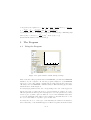
A Program for Calculating Mobility and Carrier
Density in Bulk Semiconductors
Dan Barrett, Electrical Engineering, University of Notre Dame
Contents
1 Introduction
A-1
2 Theory
A-2
3 The Program
A-4
1
3.1
Using the Program . . . . . . . . . . . . . . . . . . . . . . . . . . A - 4
3.2
Saving Plots . . . . . . . . . . . . . . . . . . . . . . . . . . . . . . A - 6
3.3
Program Details . . . . . . . . . . . . . . . . . . . . . . . . . . . A - 6
3.4
Adding Semiconductors . . . . . . . . . . . . . . . . . . . . . . . A - 7
Introduction
This program is meant to save time by providing an easy to use and automated
method for the calculation and plotting of Mobility, Carrier Concentration,
Conductivity, and the Fermi Energy in a variety of semiconductors.
2
Mobility µ( cm
V ·s ) is a measure of how well charge carriers are able to move
through a substance.
Together with carrier concentration (n for electrons, p for holes), mobility is
1
) of a substance.
important for determining the conductivity ρ( Ω·cm
ρ = qnµn + qpµp
(1)
Electrons are able to flow more quickly in materials with higher mobility. Since
the speed of an electronic device is limited by the time it takes a carrier to move
from one side to the other, devices composed of materials with higher mobility
are able to achieve higher speeds. For this reason, it is useful to maximize the
mobility of materials used.
Though methods for calculating the mobility have been practiced for years,
there has not been a tool available for calculating it automatically. Researchers
have been forced to manually go through the calculations if they want to know
what the theoretically predicted mobility of a particular semiconductor is. The
Mobility program solves this problem by providing an intuitive interface through
A-1
which a user can specify various parameters from which it calculates the mobility, along with related values such as the conductivity and carrier density.
The program is open source, and users may add any semiconductor they wish,
provided that they have the necessary data.
2
Theory
The Mobility is determined by the rate at which electrons are scattered by
impurities and defects within the crystal structure of the semiconductor. This
rate 1/τ (s− 1) is the reciprocal of the relaxation time τ (s), the average time
between collisions. The relaxation time can be adjusted to account for the
varying degrees of scattering on any given collision. This is called the momentum
relaxation time τm . The mobility is dependent upon τm by the equation
µ=
qτm
m∗
(2)
There are several mechanisms by which the electrons are scattered. Ionized
impurities interact with electrons and holes, attracting/repelling them via the
electric force. Electrons can also be scattered by neutral impurities, dislocations
in the crystal structure, and by acoustic and optical phonons. The equations
for the momentum relaxation times are given in Table 1 in the form
τi (x) = τi xri
Where x =
(3)
E
kT
The total scattering rate is equal to the sum of the individual rates.
X 1
1
=
τm (x)
τi (x)
(4)
Since these scattering rates are a function of electron energy, they must be averaged over the Fermi Dirac electron distribution. The procedure for averaging
the relaxation time over the electron distribution is
R∞
2 0 τm (x)(−∂f0 /∂x)xt+3/2 dx
t
R∞
(5)
< τm (x)x >=
3
f0 x1/2 dx
0
[1] The equation for the Fermi Dirac Distribution function f0 is
1
1 + exp(
E−Ef
kT
)
(6)
[1] where E is the electron energy, Ef is the Fermi Energy, k is Boltzmann’s
constant, and T is the Temperature.
A-2
Table 1: Momentum Relaxation Times and reduced Energy dependence for
Materials with Isotropic Parabolic Bands [1]
Scattering mechanism
τi
ri
Ionized
0.414ǫ2r (0)T 3/2
m∗ 1/2
Z 2 NI (cm− 3)g(n∗,T,x) m
3/2
Neutral
m∗ 2
8.16x106
ǫr (0)Nn (cm− 3) m
0
Deformation Potential
2.4x10−20 Cl (dyn/cm2 ) m 1/2
2 (eV )T 3/2
m∗
ξa
−1/2
Piezoelectric
9.54x10− 8
m 1/2
h214 (V /cm)(3/Cl +4/Ct )T 1/2 m∗
1/2
Deformation Potential
4.83x10−20 Cl (dyn/cm2 )[exp(θ/T )−1] m 3/2
2 (eV )T 1/2 θ
m∗
ξA
−1/2
Polar
9.61x10−15 ǫr (0)ǫr (∞)[exp(θ/T )−1] m
m∗
ǫr (0)−ǫr (∞)θ 1/2 (θ/T )r
r(θ/T )
Impurities
Acoustic Phonons
Optical Phonons
The Fermi Energy Ef is found by solving the charge neutrality equation.
N d− − N a+ = n − p
(7)
R∞
R∞
Na
x1/2 dx
x1/2 dx
−
1+exp(x−ηn ) , p = Nv 0 1+exp(x−ηp ) , N a = 1+ga exp[(Ea −Ef )/kT ] ,and
f
E −E
Nd
−Ec
and where ηn = E kT
and ηp = vkT f , N c =
N d+ = 1+gd exp([(E
f −Ed )/kT ]
∗Mh 3/2
∗Me 3/2
2( 2∗π∗k∗T
) , Nv = 2( 2∗π∗k∗T
) ,
h2
h2
where n = Nc
0
Scattering from dislocations also occurs. The momentum relaxation time τdis
2 3/2
3 2 2
(1+4λ2 K⊥
)
2
b T 1/2
where λ = ( ǫk
and k⊥
=
follows the equation τdis = N~disǫmc∗ e4
λ4
e2 n∗ )
∗
2Em
~2 [2]
Note that this program does not take the effect of dislocations on the charge
balance equation into account. This is a valid assumption when the dislocation
concentration is low.
In Table 1, NI = concentration of ionized impurities; g(n∗, T, x) = ln(1 + b) −
b/(1 + b); b = 4.31x1013 [ǫr (0)T 2 /n∗](m ∗ /m)x; Nn = concentration of neutral
impurities; Cl = 1/5(3C11 + 2C12 + 4C44 );Ct = 1/5(C11 − C12 + 3C44 );θ =
hωLO /k.
A-3
∂n
∂ηc
F−1/2 (Nc )
F1/2 (Nc ) ,
and
ηv =
Ev −Ef
kT
,
∂n
∂ηc
=n
Nd0 Nd+
Na0 Na−
Na + Nd
F
(Nv )
p F−1/2
[1]
1/2 (Nv )
∂p
+ ∂η
+
v
n∗ is given by the equation n∗ =
∂p
∂ηv
=
where ηc =
EF −Ec
,
kT
r(θ/T ) is given by r = 1−.5841θ/T +.292(θ/T )2 −.037164(θ/T )3 +.0012016(θ/T )4
.5
when (θ/T ) < 5 and by r = (3π8 ) (θ/T ).5 when (θ/T ) > 5 [3]
Additional information can be found in [1].
3
3.1
The Program
Using the Program
1
0.8
0.6
0.4
0.2
0
0
0.2
0.4
0.6
0.8
1
Figure 1: Program with the default startup settings
First of all, since this program is written in MATLAB, you must have MATLAB
installed on your computer. To run the program, simply set your MATLAB
directory to the folder which contains this program and its files, then type
”Mobility” into the MATLAB command window. This will bring up the GUI,
which should look like Figure 1.
You may input parameters into the corresponding text boxes on the upper left.
On the lower left, you have the choice to plot as a function of either one or two
different parameters. The specific value input above for the parameter you have
chosen to plot by will be ignored. There is a box for the minimum value and a
box for the maximum value taken by the parameter. Beneath these two boxes
is a box for the number of points to plot on that axis.
You may also choose to view a plot of the Mobility, the Carrier Concentration,
the Conductivity, or the Fermi Energy level. There is a pull down menu for this.
A-4
The check boxes enable you to select which individual plots you wish to see,
such as the mobility from particular scattering mechanisms.
You may also choose how to scale the graph. You may choose either linear or
logarithmic graphs for any combination of X, Y, and Z axes. The Z axis is only
used when plotting with respect to two different parameters, which results in a
3D graph. The graph rotation bars also only work under this circumstance.
You may choose to have the program auto-fit the graph, or you may choose
your own limits. When you are ready to calculate, simply press the ”Calculate”
button.
Mu (cm2/V*s)
Take Note: At extremely high doping densities, the electron clouds of the impurities begin to overlap, and cause additional conduction. This program does
not account for this, so use caution when applying this program to extremely
high doping levels.
6
10
5
10
1
2
10
10
T (K)
Figure 2: In the above example, we have chosen to calculate the Mobility of
GaAs as a function of Temperature from 2 K to 300 K. Both the X and Y axes
are logarithmic, and we have chosen to view the plot with X ranging from 0 to
180 and with Y ranging from 4 x 104 to 6 x 106 .
A-5
3.2
Saving Plots
To save a plot, click File- Save As in the menu bar at the top of the Mobility
window. You can then pick whatever file type, name, and location you want.
You are done, but the saved file may have an ugly white background which
effects the look of the buttons etc.
There is an optional step which will fix this. Click File- Export Setup. This will
open up a window. Go to the Rendering section,and uncheck the custom color
checkbox. Save again.
In addition, if you wish to access the raw data generated by the program, you
can access it in the data.txt file. Each column in the file is a variable. They are
stored in the following order:
µ, the total mobility,
µI , the mobiliity from ionized impurities,
µN , the mobility from neutral impurities,
µAD , the mobility from accoustic deformation,
µAP , the mobility from accoustic piezoelectric scattering,
µOD , the mobility from optical deformation,
µOP , the mobility from optical polar scattering,
µDIS ,the mobility from dislocation scattering,
n, the free electron concentration,
NA− , the concentration of ionized acceptor impurities,
+
, the concentration of ionized donor impurities,
ND
p, the hole concentration,
ρ, the conductivity,
Ef , the Fermi Energy,
NN , the concentration of neutral impurities,
EG , the energy gap level.
3.3
Program Details
In order to aid in the understanding of the program and facilitate additions and
modifications, I have included a description of the workings of the program.
Included in the folder are the following files: Mobility.m mucalc.m Efcalc.m Mobilityfunct.m FDdata.mat Mobilitynew.m plotter.m FDsolver.m data.txt Lookup.m
Mobility.fig datachart.m
Mobility.m and Mobilitynew.m are MATLAB generated files which create the
GUI interface and call Mobilityfunct.m and Plotter upon actions by the user.
Mobilityfunct.m retrieves parameters from the GUI and creates the neccessary
arrays for plotting. It then sends this information to mucalc.m.
mucalc.m is the main calculation function. It retrieves the proper data from
datachart.m and FDdata.mat, then retrieves the Fermi level and carrier concentrations from Efcalc.m. With this information, mucalc.m then calculates the
mobility, saves the data to data.txt and then sends all data back to Mobility-
A-6
funct.m.
Mobilityfunct.m prepares the data for plotting, and then sends it to Plotter.m,
which plots it. Plotter.m also runs upon the change of an input on the GUI
which affects the plot, but does not require additional calculation.
The file FDsolver.m is a program which numerically solves the Fermi Dirac
integral and stores the result in FDdata.mat. The Lookup.m file is used by
Efcalc.m to retrieve data from FDdata.mat.
The quad Function
The quad and quadv functions are built-in MATLAB numerical integration functions. They are utilized in solving the Fermi-Dirac Integral in the FDsolver.m
program, and for averaging the relaxation time over the electron distribution in
mucalc.m. The difference between the two is that quad returns a single value,
while quadv returns a vector.
3.4
Adding Semiconductors
It is possible that you may want to use this program for a semiconductor which
is not yet included. In order to add a semiconductor, first type ’guide’ into the
MATLAB command window. This will open the MATLAB GUI editor. Click
on the ”Open Existing GUI” tab, then click ’browse’. Find the folder which
contains the files of this program, and select Mobility.fig.
You should now be looking at the figure file for the program GUI. Double
click on the pull down menu labeled GaN. This will open the GUIDE property
inspector for that menu. Find the ’string’ field, open it, and add the name of
the Semiconductor you wish to add at the bottom of the list.
Now that you have added your semiconductor to the pull-down menu, it is time
to add some functionality to it. Open the file datachart.m. This file contains
the data specific to each semiconductor [1]. This data is stored in a matrix, each
of whose rows represents a semiconductor. Each column contains the values of a
particular variable for each semiconductor. When running the program, the pull
down menu from which you choose a semiconductor produces a number which
corresponds to the placement of the semiconductor which you have chosen. The
program then uses the values in the matrix from the row with an index equal
to that number. For example, if you choose GaN, which is at the top of the list,
the menu produces a 1, and uses the values from the 1st (top) row.
Whether you are replacing an existing semiconductor, or adding another, it is
important that your data and the name you added to the menu each are the
same number of rows from the top in their respective lists so that the program
does indeed use the data corresponding to that semiconductor.
When adding a row of data, simply use the same syntax as the rest of the rows:
use spaces between elements in the row, and end the row in either a ’;...’ if it is
not the last row, or a ’]’ if it is. The whole matrix should have the form
A-7
[x x x;...
x x x;...
x x x]
After adding the row to the data chart and adding the name to the menu, you
are now ready to use the program for your new semiconductor.
References
[1] C. M. e. a. Wolfe, Physical Properties of Semiconductors. Englewood Cliffs,
N. J.: Prentice Hall, 1989.
[2] J. R. S. D. C. Look, “Dislocation Scattering in GaN,” Physical Review Letters, 1999.
[3] D. C. Look, Electrical Characterization of GaAs Materials and Devices. New
York NY: John Wiley and Sons, 1989.
A-8