1
User’s Manual Model ISC450G [Style: S2] Inductive Conductivity Converter IM 12D06D05-01E 3rd Edition Note This page may be referred to when reading pages where subsequent submenu screens are shown in the text. Connection to the relevant submenu screen is indicated by a doted line with an arrow. Note that screens in the text are typical examples and actual screens may differ depending on the set parameters. Commissioning Connection to the relevant submenu screen is indicated by a doted line with an arrow. Measurement setup Measure Conductivity only Configure sensor Temperature settings Temp. Compensation Calibration settings Concentration Enter PREFACE Electrostatic discharge The EXAxt converter contains devices that can be damaged by electrostatic discharge. When servicing this equipment, please observe proper procedures to prevent such damage. Replacement components should be shipped in conductive packaging. Repair work should be done at grounded workstations using grounded soldering irons and wrist straps to avoid electrostatic discharge. WARNING Installation and wiring The EXAxt converter should only be used with equipment that meets the relevant IEC, American or Canadian standards. Yokogawa accepts no responsibility for the misuse of this unit. CAUTION The Instrument is packed carefully with shock absorbing materials, nevertheless, the instrument may be damaged or broken if subjected to strong shock, such as if the instrument is dropped. Handle with care. WARNING • Do not use an abrasive or organic solvent in cleaning the instrument. • Do not modify the ISC450G converter. • Substitution of components may impair suitability for Division 2. Do not remove or replace while circuit is live unless area is know to be non-hazardous. Explosion Hazard – Do not disconnect equipment unless area is known to be nonhazardous. Do not reset circuit breaker unless power has been removed from the equipment or the area is known to be non-hazardous. Notice • This manual should be passed on to the end user. • The contents of this manual are subject to change without prior notice. • The contents of this manual shall not be reproduced or copied, in part or in whole, without permission. • This manual explains the functions contained in this product, but does not warrant that they are suitable the particular purpose of the user. • Every effort has been made to ensure accuracy in the preparation of this manual. However, when you realize mistaken expressions or omissions, please contact the nearest Yokogawa Electric representative or sales office. • This manual does not cover the special specifications. This manual may be left unchanged on any change of specification, construction or parts when the change does not affect the functions or performance of the product. • If the product is not used in a manner specified in this manual, the safety of this product may be impaired. Yokogawa is not responsible for damage to the instrument, poor performance of the instrument or losses resulting from such, if the problems are caused by: • Improper operation by the user. • Use of the instrument in improper applications • Use of the instrument in an improper environment or improper utility program • Repair or modification of the related instrument by an engineer not authorized by Yokogawa. Safety and Modification Precautions • Follow the safety precautions in this manual when using the product to ensure protection and safety of the human body, the product and the system containing the product. ii The following safety symbols are used on the product as well as in this manual. DANGER This symbol indicates that an operator must follow the instructions laid out in this manual in order to avoid the risks, for the human body, of injury, electric shock, or fatalities. The manual describes what special care the operator must take to avoid such risks. WARNING This symbol indicates that the operator must refer to the instructions in this manual in order to prevent the instrument (hardware) or software from being damaged, or a system failure from occurring. CAUTION This symbol gives information essential for understanding the operations and functions. Note! This symbol indicates information that complements the present topic. This symbol indicates Protective Ground Terminal This symbol indicates Function Ground Terminal (Do not use this terminal as the protective ground terminal.) This symbol indicates Alternating current. This symbol indicates Direct current. Warranty and service Yokogawa products and parts are guaranteed free from defects in workmanship and material under normal use and service for a period of (typically) 12 months from the date of shipment from the manufacturer. Individual sales organisations can deviate from the typical warranty period, and the conditions of sale relating to the original purchase order should be consulted. Damage caused by wear and tear, inadequate maintenance, corrosion, or by the effects of chemical processes are excluded from this warranty coverage. In the event of warranty claim, the defective goods should be sent (freight paid) to the service department of the relevant sales organisation for repair or replacement (at Yokogawa discretion). The following information must be included in the letter accompanying the returned goods: • Part number, model code and serial number • Original purchase order and date • Length of time in service and a description of the process • Description of the fault, and the circumstances of failure • Process/environmental conditions that may be related to the failure of the device. • A statement whether warranty or nonwarranty service is requested • Complete shipping and billing instructions for return of material, plus the name and phone number of a contact person who can be reached for further information. Returned goods that have been in contact with process fluids must be decontaminated/disinfected before shipment. Goods should carry a certificate to this effect, for the health and safety of our employees. Material safety data sheets should also be included for all components of the processes to which the equipment has been exposed. iii TABLE OF CONTENTS PREFACE 1. INTRODUCTION AND GENERAL DESCRIPTION .....................................................1 1-1. Instrument check ...................................................................................................1 1-2. Application .............................................................................................................1 2. GENERAL SPECIFICATIONS OF EXAxt ISC450G ....................................................2 3. INSTALLATION AND WIRING.....................................................................................5 3-1. Installation and dimensions ...................................................................................5 3-1-1. Installation site ..........................................................................................5 3-1-2. Mounting methods.....................................................................................5 3-2. Wiring ....................................................................................................................7 3-2-1. Preparation ................................................................................................7 3-2-2. Cables, Terminals, glands and conduit adapter .......................................8 3-3. Wiring the power supply ........................................................................................9 3-3-1. General precautions ..................................................................................9 3-3-5. Grounding the housing ............................................................................10 3-3-6. Switching on the instrument ....................................................................10 3-3-2. Access to terminal and cable entry .........................................................10 3-3-3. AC power ................................................................................................10 3-3-4. DC power ................................................................................................10 3-4. Wiring the contact signals.................................................................................... 11 3-4-1. General precautions ................................................................................11 3-4-2. Contact outputs .......................................................................................11 3-4-3. Contact input ...........................................................................................11 3-5. Wiring the mA-output signals............................................................................... 11 3-5-1. General precautions ................................................................................11 3-5-2. Analog output signals ..............................................................................11 3-6. Wiring the sensor.................................................................................................12 3-6-1. General precautions ................................................................................12 3-6-2. Connecting the sensor cable to the converter ........................................12 3-6-3. Installation of the sensor .........................................................................12 3-6-4. Sensor cable connections using junction box (BA10) and extension cable (WF10) ..........................................................................13 IM 12D06D05-01E 3rd Edition: Aug. 2008 (YK) All Rights Reserved, Copyright © 2007, Yokogawa Electric Corporation IM 12D06D05-01E iv 4. OPERATION OF EXAxt ISC450G .............................................................................16 4-1. Main display functions .........................................................................................16 4-2. Trending graphics ................................................................................................16 4-3. Zoom in on details ...............................................................................................16 4-3-1. Actual mA1 ..............................................................................................17 4-3-2. Actual mA2 ..............................................................................................17 4-3-3. S1/S2/S3/S4 ............................................................................................17 4-3-4. C.C. (factory). ..........................................................................................17 4-3-5. C.C. (adjusted) ........................................................................................17 4-3-6. Temp. comp 1 .........................................................................................17 4-3-7. Temp. comp 2 .........................................................................................17 4-3-8. Sensor ohms. ..........................................................................................17 4-3-9. Last calibrated at .....................................................................................17 4-3-10. Calibration due at ..................................................................................17 4-3-11. Projected calibration at .........................................................................17 4-3-12. HART ID ................................................................................................17 4-3-13. Software revision...................................................................................18 4-3-15. Logbook ................................................................................................18 4-3-16. Trouble shooting ..................................................................................18 4-4. Information function .............................................................................................18 4-5. Setup-Calibration & commissioning.....................................................................18 4-6. Secondary- primary value display switch ............................................................18 4-7. Navigation of the menu structure ........................................................................19 5.MENU STRUCTURE COMMISSIONING ....................................................................20 5-1. Configure sensor ................................................................................................20 5-2. Temperature setting .............................................................................................20 5-3. Temperature compensation .................................................................................20 5-4. Calibration settings ..............................................................................................22 5-5. Concentration ......................................................................................................22 5-6. mA output setup...................................................................................................24 5-7. Contact output setup ...........................................................................................26 5-8. Fail .......................................................................................................................28 5-9. Simulate...............................................................................................................28 5-10. Input contacts ....................................................................................................28 5-11. Error configuration .............................................................................................30 5-12. Logbook configuration .......................................................................................30 5-13. Advanced setup .................................................................................................32 5-14. Display setup .....................................................................................................34 IM 12D06D05-01E v 6. CALIBRATION ...........................................................................................................36 7. MAINTENANCE .........................................................................................................38 7-1. Periodic maintenance .........................................................................................38 7-2. Periodic maintenance of the sensor ....................................................................38 7-3. Cleaning methods................................................................................................38 7-4. Contrast adjustment ............................................................................................38 8. TROUBLESHOOTING ...............................................................................................39 8-1. General ...............................................................................................................39 8-2. Calibration check .................................................................................................39 8-3. Predictive maintenance .......................................................................................39 8-4. Poor calibration technique ...................................................................................39 8-5. Error displays and actions ...................................................................................39 9. QUALITY INSPECTION .............................................................................................40 10. SPARE PARTS ........................................................................................................44 APPENDICES ................................................................................................................45 APPENDIX 1 Temperature compensation ..................................................................45 APPENDIX 2 Temperature compensation matrix. ......................................................48 APPENDIX 3 Calibration solutions for conductivity ....................................................49 APPENDIX 4 Measurement principle ........................................................................50 APPENDIX 5 HART HHT (275/375) Menu structure ..................................................51 APPENDIX 6 Control drawing for FM approval ..........................................................55 Customer Maintenance Parts List (for Style: S2) ......................CMPL 12D06D05-02E Revision Record ..............................................................................................................i IM 12D06D05-01E vi 1 The Yokogawa EXAxt ISC450G is a converter designed for industrial process monitoring, measurement and control applications. This instruction manual contains the information needed to install, set up, operate and maintain the unit correctly. This manual also includes a basic troubleshooting guide to answer typical user questions. Yokogawa can not be responsible for the performance of the EXAxt converter if these instructions are not followed. 1-1. Instrument check Upon delivery, unpack the instrument carefully and inspect it to ensure that it was not damaged during shipment. If damage is found, retain the original packing materials (including the outer box) and then immediately notify the carrier and the relevant Yokogawa sales office. Make sure the model number on the nameplate affixed to the top of the instrument agrees with your order. Example of the nameplate is shown below. INDUCTIVE CONDUCTIVITY TRANSMITTER MODEL SUFFIX ISC450G SUPPLY OUTPUTS AMB. TEMP. STYLE NO. 4-20mA(mA1: +HART) -20 to +55°C CL I, DIV 2, GROUPS ABCD T6 FOR Ta -20 to +55°C SEE INSTRUCTION MANUAL TYPE 4X SEE CONTROL DRAWING NFM016-A9 P.1 1-2. Application The EXAxt converter is intended to be used for continuous on-line measurement of Conductivity and/or Concentration in industrial installations. The unit combines simple operation and microprocessor-based performance with advanced self-diagnostics and enhanced communications capability to meet the most advanced requirements. The measurement can be used as part of an automated process control system. It can also be used to indicate operating limits of a process, to monitor product quality, or to function as a controller for a dosing/dilution system. Sensors should normally be mounted close to the converter in order to ensure easy calibration and peak performance. If the unit must be mounted remotely from the sensors, WF10 extension cable can be used, up to a maximum of 50 metres (150 feet), with a BA10 junction box, and up 10 metres standard sensor cable. The EXAxt is delivered with a general purpose default setting for programmable items (see Chapter 5). While this initial configuration allows easy start-up, the configuration should be adjusted to suit each particular application. An example of an adjustable item is the type of temperature sensor used. The EXAxt can be adjusted for a number of different types of temperature sensors. Details provided in this instruction manual are sufficient to operate the EXAxt with all Yokogawa sensor systems and a wide range of third-party commercially available probes. For best results, read this manual in conjunction with the corresponding sensor instruction manual. R C US Made in Japan N200 Figure 1-1. Nameplate Note! The nameplate will also contain the serial number and any relevant certification marks. Be sure to apply correct power to the unit, as detailed on the nameplate. Yokogawa designed the EXAxt converter to withstand industrial environments. It meets all the CE regulatory standards. The unit meets or exceeds stringent requirements (see section 2) without compromise, to assure the user of continued accurate performance in even the most demanding industrial installations. IM 12D06D05-01E 1 INTRODUCTION AND GENERAL DESCRIPTION 1. INTRODUCTION AND GENERAL DESCRIPTION 2 2. GENERAL SPECIFICATIONS OF EXAxt ISC450G A) Input specifications : Compatible with the Yokogawa inductive conductivity ISC40 series with integrated temperature sensor: NTC30k or Pt1000 B) Input range Conductivity Minimum Maximum Temperature Cable length : : : : : 0 to 1999 mS/cm at 25 °C (77 °F) reference temperature 1 μS/cm (at process temperature) 2 S/cm (at process temperature) -20 to +140 ºC (0 to 280 ºF) max. 60 metres (200 feet) 10 metres (35 feet) fixed sensor cable + 50 metres (165 feet) WF10 extension cable. Influence of cable can be adjusted by doing an AIR CAL with the cable connected to a dry cell C) Accuracy (under reference conditions): Conductivity : ≤ 0.5 % of reading ± 1.0 μS/cm Temperature : ≤ 0.3ºC (0.6ºF) Temp.compensation: ≤1 % for NaCl, ≤ 3 % for Matrix Step response : ≤ 4 seconds for 90 % (for a 2 decade step) Note on performance specifications The following tolerance is added to above performance. mA output tolerance: ±0.02 mA of “4-20 mA“ D) Transmission signals General : Two isolated outputs of 4-20 mA. DC with common negative. Maximum load 600Ω. Bi-directional HART® digital communication, superimposed on mA1 (4-20 mA) signal. Output function : Linear or 21-step table for Conductivity, Concentration or Temperature. Control function : PID control. Burn out function : Burn up (21.0 mA) or burn down (3.6 mA) to signal failure. acc. NAMUR NE43. Parameters : Adjustable damping : Expire time Hold : The mA-outputs are frozen to the last/fixed value during calibration/ commissioning Cond. range : min span 10 μs/cm≥10% of high valve (20 mA) max span 1999 mS/cm E) Contact outputs General Switch capacity Status Control function IM 12D06D05-01E : Four SPDT relay contacts with display indicators : Maximum values 100 VA, 250 VAC, 5 Amps. (*) Maximum values 50 Watts, 250 VDC, 5 Amps. (*) : High/Low process alarms, selected from conductivity, concentration or temperature. Configurable delay time and hysteresis : PID duty cycle or pulsed frequency control : FAIL alarm : On / Off : Adjustable damping : Expire time 3 Hold : Contact can be used to signal the HOLD situation. Fail safe : Contact S4 is programmed as fail-safe contact. (*)Note: When contact output current is more than 4 Amps, ambient temperature should be less than 40 ºC. Contact closed : Remote range switching to 10 times the programmed range. : If impedance > 100 kΩ: "Range1, 2" (“Programmed range for mA1 and mA2 output" is "Range1, 2.”) : If impedance < 10 Ω: 10 x “Range1, 2" G) Temperature compensation Function : Automatic or manual, for temperature ranges mentioned under B (inputs). Reference temp. : Programmable from 0 to 100 ºC or 30 - 210 ºF (default 25 ºC). H) Calibration : Semi-automatic calibration using pre-configured OIML (KCl) buffer tables, with automatic stability check Manual adjustment to grab sample * Organisation Internationale de Metrologie Legale, international recommendation nr. 56 standard solutions reproducing the conductivities of electrolytes, 1981. I) Logbook : Software record of important events and diagnostic data readily available in the display or through HART®. J) Display : Graphical Quarter VGA (320 x 240 pixels) LCD with LED backlight and touchscreen. Plain language messages in English, German, French, Spanish, Italian, Swedish, Portuguese and Japanese. K) Shipping details Package size Package weight Converter weight : 290 x 300 x 290 mm (L x W x D) (11.5 x 11.8 x 11.5 inch) : app. 2.5 kg (5.5 lbs) : app. 1.5 kg : Cast aluminum housing with chemically resistant coating; Polycarbonate cover with Polycarbonate flexible window : Protection IP66 / NEMA 4X / CSA Type 3S Colour : Silver grey ISC450-A(D)-A : IP66 cable glands are supplied with the unit ISC450-A(D)-U : NEMA 4X close up plugs are mounted in the unused cable entry holes and can be replaced by conduit fittings as required Pipe, Panel or Wall mounting using optional hardware Optional conduit adapter G1/2, 1/2NPT or M20 female M) Power supply ISC450G-A : Ratings; 100-240 V AC Acceptable range; 90 to 264 V AC Ratings; 50/60 Hz Acceptable range; 50 Hz ±5%, 60 Hz ±5% Power Consumption; 15 VA ISC450G-D : Ratings; 12-24 V DC Acceptable range; 10.8 to 26.4 V DC Power Consumption; 10 W L) Housing IM 12D06D05-01E 2 GENERAL SPECIFICATIONS F) Contact input Contact open 4 N) Safety and EMC conforming standards Safety : EN 61010-1 CSA C22.2 No.61010-1 UL 61010-1 FM3611 Class I, Div.2, Group ABCD,T6 for Ta -20 to 55ºC EMC : conforms to EN61326 Class A, AS/NZS CIPR 11 Installation altitude: 2000 m or less Category based on IEC 61010: II (Note) Pollution degree based on IEC 61010: 2 (Note) Note: Installation category, called over-voltage category, specifies impulse withstand voltage. Category II is for electrical equipment. Pollution degree indicates the degree of existence of solid, liquid, gas or other inclusions which may reduce dielectric strength. Degree 2 is the normal indoor environment. O) Environment and operational conditions Ambient temperature: -20 to +55 ºC (-5 - 130 ºF) Storage temperature: -30 to +70 ºC (-20 - 160 ºF) Humidity : 10 to 90% at 40 ºC (100 ºF) RH (non-condensing) Data protection : EEPROM for configuration data and logbook. Lithium cell for clock Watchdog timer : Checks microprocessor Power down : Reset to measurement Automatic safeguard: Auto return to measuring mode when touchscreen is untouched for 10 min. Model and Suffix Codes [Style: S2] Model Suffix code Option code Description ISC450G ----------------- ----------------- Inductive conductivity Converter Power -A -D --------------------------------- AC version (100…240 VAC) DC version (12…24 VDC) --------------------------------- General purpose version FM version Type -A -U Mounting Hardware /UM /U /PM Hood /H5 Conduit adapter /AFTG /ANSI /AM20 Tag Plate /SCT Universal mounting kit (panel, pipe, wall) Pipe and wall mounting hardware (*2) Panel mounting hardware (*2) Awning hood (stainless steel) (*2) G1/2 (*2) 1/2NPT (*2) M20 (*2) Stainless steel tag plate (*1) *1 If the tag number is predefined with the purchase, Yokogawa will inscript the tag plate with the specified tag number, and program the tag number in the converter. *2 Option codes /U, /PM, /H5, /AFTG, /ANSI and /AM20 are not specified for FM version (-U). IM 12D06D05-01E 5 3. INSTALLATION AND WIRING The ambient temperature and humidity of the installation environment must be within the limits of the instrument specifications. (See chapter 2). 3-1-2. Mounting methods Refer to figures 3-2 and 3-3. Note that the EXAxt converter has universal mounting capabilities: • Panel mounting using optional brackets • Surface mounting on a plate (using bolts from the back) • Wall mounting on a bracket (for example, on a solid wall) • Pipe mounting using a bracket on a horizontal or vertical pipe Size nominal 50A Unit: mm (inch) F Hood (Option code: /H5, some cutout on the left side cover) 184(7.2") 220(8.66") 144(5.67") 72(2.8") 24.5(1") 144(5.67") 20 (0.79") M20 cable gland (When shipped, not installed) 20 (0.79") 121.5(4.78") A D B C E F A : For output signal Adapter B : For contact input C : For sensor cable D : For contact output (S1 and S2) E : For contact output (S3 and S4) F : For power supply Grounding terminal (M4 screw) Figure 3-1. F Adapter for Coduit Work (optional) (option code : / AFTG, / ANSI, / AM20) Approx. 49 (1.93") 55(2.2") F G1/2 screw (/AFTG), F 1/2 NPT screw (/ANSI) F M20 screw (/AM20) Housing dimensions and layout of glands IM 12D06D05-01E 3 INSTALLATION AND WIRING 3-1. Installation and dimensions 3-1-1. Installation site The EXAxt 450 converter is weatherproof and can be installed inside or outside. It should, however, be installed as close as possible to the sensor to avoid long cable runs between sensor and converter. In any case, the cable length should not exceed 60 metres (200 feet). Select an installation site where: • Mechanical vibrations and shocks are negligible • No relay/power switches are in the direct environment • Access is possible to the cable glands (see figure 3-1) • The converter is not mounted in direct sunlight or severe weather conditions • Maintenance procedures are possible (avoiding corrosive environments) 6 Unit: mm (inch) +1 138 0 (5.43") min.195(7.75") min.185 (7.25") +1 138 0 (5.43") 138(5.43") M6 138 (5.43") M5 M6 Figure 3-2. Option /PM: panel mounting diagram (Note) When option code "/UM" is specified, universal pipe/wall/pannel mounting kit are supplied--same as option code "/U" and "/PM" both specified. wall mounting 13 (0.51") 80 (3.15") pipe mounting (vertical) pipe mounting (horizontal) 2x Ф6.5 (0.26") 200 (7.87") 4x Ф10 (0.4") 35 (1.38") 15 (0.6") 70 (2.75") 154.5 (6.08") 2" ND. pipe Figure 3-3. Option /U: wall and pipe mounting diagram IM 12D06D05-01E WARNING This connector for software must be used only by 7 Yokogawa’s servicefor personnel. connector (future) software input terminal block potentiomerter LCD bracket protective shield bracket 6 X M20 glands Note: ISC450G-A(D)-U The enclosure is provided with stoppers in stead of M20 cable glands for the unused holes. These stoppers must be removed and replaced by FM approved conduit fittings in accordance with good installation practice. See APPENDIX 6, Control drawing for FM approval. Figure 3-4. Internal view of EXAxt wiring compartment 3-2. Wiring 3-2-1. Preparation Refer to figure 3-4. The relay contact terminals and power supply connections are under the screening (shielding) plate. These should be connected first. Connect the sensor, outputs and HART® communication connections last. To open the EXAxt 450 for wiring: 1. Loosen the four frontplate screws and swing open the cover. 2. The upper terminal strip is now visible. 3. Remove the screen (shield) plate covering the lower terminal strip. 4. Connect the power supply and contact outputs. Use the three glands at the back for these cables. DANGER • Cables that withstand temperatures of at least 70 °C should be used for wiring. • Wiring work should be performed to meet IP66 or higher requirements. Tighten four frontplate screws to 1.5 N·m torque. WARNING Always place the screen plate over the power supply and contact terminals for safety reasons and to avoid interference. 5. Put back (replace) the screen (shield) plate over the lower terminals. 6. Connect the analog output(s), the sensor inputs, and, if necessary, the HART® wiring and input contact. 7. Use the front three glands for analog output, sensor inputs, contact input and HART® wiring (see figure 3-5). 8. Swing back the cover and secure it with the four screws. 9. Switch on the power. Commission the instrument as required or use the default settings. CAUTION Do not turn on power with the touchcsreen pressed, otherwise inaccurate screen positioning will occur. If it occurs, leave the touchscreen unpressed, turn off power then on again. The screen positioning will be accurate. IM 12D06D05-01E 3 INSTALLATION AND WIRING output terminal block 8 3-2-2. Cables, Terminals, glands and conduit adapter ISC450G-A(D)-A The ISC450 is supplied with terminals suitable for the connection of finished wires in the size range of 0.13 to 2.5 sq.mm. (26 to 14 AWG). The cable glandes supplied will form a tight seal on cables with an outside diameter of 6 to 12 mm (0.24 to 0.47 inches). Unused cable entry holes must be sealed with cable glands including the blind plugs supplied. ISC450G-A(D)-U The ISC450 is supplied with terminals suitable for the connection of finished wires in the size range of 14- 26 AWG. The cable entry holes are sealed with FM certified plugs. Prior to cable entry the plugs can be removed with allen key size 3/8” The cable conduit fittings can be mounted in the holes of the housing as required. The cable glands supplied with the unit will give a tight seal on cables with outside diameter of 0.24 to 0.47 inches. High voltage section Contact (S1, S2) output cables mA cables Contact (S3, S4) output cables Input contact Power cable Sensor Cables Suitable for cables with an outside diameter between 6 - 12 mm (0.24 - 0.47”) Figure 3-5a. Cable glands diagram Gland nut Contents: 6 X Gland M20 6 X Close up plug 6 X Gland nut M20 6 X O-ring 17.12 X 2.62 EPDM 70° sh. O-ring NOTE: The glands must be installed properly to meet IP66 and NEMA 4X rating. Use close up plug for unused glands. Gland Close up plug Figure 3-5b. How to install cable glands IM 12D06D05-01E NOTE: Moisturize O-ring before assembling. 9 Adapter for conduit work When protect the cable with a conduit, replace the M20 cable gland with a cable gland of optional conduit adapter, and set the adapter shown as Figure 3-5c. Nut Unit: mm(inch) Packing G1/2 screw (/AFTG), 1/2 NPT screw (/ANSI) M20 screw (/AM20) Adapter Figure 3-5c. Conduit adapter FRONT GLANDS REAR GLANDS Sensor mA1 HART Power output signals Contact output S1 S2 Contact output mA2 S3 S4 Contact input Figure 3-6. System configuration 3-3. Wiring the power supply 3-3-1. General precautions Make sure the power supply is switched off. Also, make sure that the power supply is correct for the specifications of the EXAxt and that the supply agrees with the voltage specified on the textplate. 1. 2. 3. DANGER Install an external switch or circuit breaker to the power supply of the converter. Use an external switch or circuit breaker rated 5A and conforming to IEC 60947-1 or IEC 60947-3. It is recommended that the external switch or circuit breaker be installed in the same room as the converter. 4. 5. The external switch or circuit breaker should be installed within reach of the operator and identified with marking as a power supply switch to the converter. Power lines such as power cables and contact outputs should be fixed securely onto a wall or construction using cable racks, conduit tubing, nylon bands or other appropriate ways. Accidental removal from terminals by pulling may result in electric shock. Local health and safety regulations may require an external circuit breaker to be installed. The instrument is protected internally by a fuse. The fuse rating is dependent on the supply to the instrument. The 250 VAC fuses should be of the “time-lag” type, conforming to IEC127. IM 12D06D05-01E 3 INSTALLATION AND WIRING Approx. 55(2.2") 49 (1.93") 10 WARNING Fuse replacement should be performed only by a qualified service person. See Sec.7. MAINTENANCE, Fuse. 3-3-3. AC power Connect terminal L to the phase line of the AC power and terminal N to the zero line. See figure 3-8 for the power ground. 3-3-4. DC power Connect terminal 1 to the positive outlet and terminal 2 to the negative outlet. Fuse ratings: Power supply Fuse type 12-24VDC, 10W max 2A/250V, Slow 100-240VAC, 15VA max 0.5A/250V, Slow 3-3-2. Access to terminal and cable entry Terminals 1 and 2 are used for the power supply. Guide the power cables through the gland closed to the power supply terminals. The terminals will accept wires of 2.5 mm2 (14 AWG). Always use cable finishings if possible. The size of conductors should be at least 1.25 mm2. The overall cable diameter should be between 7 & 12 mm. 2 - 1 2 + 1 N POWER L POWER 12-24 V /10 W FUSE: 2A/250 VAC/T 100-240 VAC/15 VA/ 50/60Hz FUSE: 500 mA/250 VAC/T DC 32 31 33 42 41 43 NC C NO NC C NO S1 63 SHLD 66 - 65 + mA2 S2 62 61 + mA1 22 250V / 5A 52 AC / DC 100VA / 50W NC CONTACTS 21 (+HART) 11 12 + TEMP 51 53 72 71 73 C NO NO C NC S3 S4 (fail-safe) 13 17 RECEIVE CONTACT SENSOR(S) mA OUTPUTS REFER TO INSTRUCTION MANUAL FOR CONNECTIONS Figure 3-7. AC 14 SHLD 16 15 DRIVE COILS ISC Input and output connections 3-3-5. Grounding the housing For the safety of the user and to protect the instrument against interference, the housing must always be connected to ground. This has to be done by a large area conductor. This cable can be fixed to the rear of the housing or by using the internal ground connections using a braided wire cable. See figure 3-8. DANGER The minimum cross sectional area of the protective grounding wire should be 0.75 mm2. IM 12D06D05-01E 3-3-6. Switching on the instrument After all connections are made and checked, the power can be switched on from the power supply. Make sure the LCD display comes on. After a brief interval, the display will change to the measured value. If errors are displayed or a valid measured value is not shown, consult the troubleshooting section (Chapter 8) before calling Yokogawa. 11 (M4 screw) N 1 L POWER 100-240 VAC/15 VA/ 50/60Hz FUSE: 500 mA/250 VAC/T AC (M4 screw) Figure 3-8-a. External grounding 3-4. Wiring the contact signals 3-4-1. General precautions The contact output signals consist of voltage-free relay contacts for switching electrical appliances (SPDT). They can also be used as digital outputs to signal processing equipment (such as a controller or PLC). It is possible to use multi-core cables for the contact in and output signals and shielded multi-core cable for the analog signals. 3-4-2. Contact outputs The EXAxt 450 unit’s four contacts (switches) that can be wired and configured to suit user requirements. Contact S4 is programmed as a fail-safe contact. Please refer to section 5-7, Contact output setup for functionality description. Alarm (limits monitoring) Contacts configured as “ALARM” can be energized when limits are crossed. Fail Contacts configured as “FAIL” will be energized when a fail situation occurs. Some fail situations are automatically signaled by the internal diagnostics (electronics) of the converter. Others can be configured by the user (see section 5-11 Error Configuration). By pressing the “INFO” button on the main screen the user is given an explanation as well as a remedy for the current fail situation. Always connect the fail contact to an alarm device such as a warning light, alarm bell or displayed on an annunciator. Figure 3-8-b. Internal grounding “ALARM” Contact “FAIL” Contact Power Off NC NC Power On NC NC Alarm NO NC Fail NC NO Fail and Alarm NC* NO HOLD NC NC * When a fail situation occurs which is related to the parameter associated with the contact (Conductivity, Concentration or temperature) the contact will go to NC. When the fail situation is not related to the parameter associated with the contact the contact will remain in the state it is currently in. 3-4-3. Contact input It is necessary to use screening/shielding on the input signal cables. Terminal 63 is used to connect the shielding. 3-5. Wiring the mA-output signals 3-5-1. General precautions The analog output signals of the EXAxt transmit low power standard industry signals to peripherals like control systems or strip-chart recorders (Figure 3-6). 3-5-2. Analog output signals The output signals consist of active current signals of 4-20 mA. The maximum load can be 600 ohms on each. IM 12D06D05-01E 3 INSTALLATION AND WIRING 2 12 It is necessary to use screening/shielding on the output signal cables. Terminal 63 is used to connect the shielding. 3-6. Wiring the sensor 3-6-1. General precautions The sensor cable transmits low voltage, high frequency signals and should be installed separately from any high voltage, high current and/or power switching cables. This is to avoid any unintentional cross talk or other kind of interference of the conductivity measurement. 3-6-2. Connecting the sensor cable to the converter 1. To access terminals remove the front cover of the EXAxt ISC450G by releasing the 4 captive screws. 2. Loosen the cable gland and pull the cable in the connection compartment. 3. The sensor leads are numbered and the leads must be connected to the terminals with the corresponding number, refer to Fig. 3-4: the temperature compensator with 11/12 - the drive coil with 15/16 - the receive coil with 13/17 Terminal 14 is for connection of the shield. 4. Screw the cable gland tight to ensure IP66 (NEMA 4X) environmental protection. An optional protection hose (flexible conduit) is available for additional mechanical protection of the sensor cable. Figure 3-9a. Dimensions IM 12D06D05-01E 3-6-3. Installation of the sensor The Model ISC40 is a “doughnut” shaped sensor. Preferably, the process will flow through the hole of the donut with the temperature compensator up-stream. For minimal obstruction of the flow and for accurate measurement without the need for calibration of the cell constant, the process will flow freely around the doughnut, allowing a minimum distance of 25 mm (1”) between doughnut and process piping (d). The sensor is provided with a gasket and retaining nut. This allows “bulkhead mounting” in tank wall or standard flange through a hole of 27 mm (1.1”) diameter (A). The insertion is 125 mm under the flange. Two flats are provided with wrench size 20 mm (0.8”) to allow easy mounting and alignment of the sensor. The model identification on one flat aligns with the “up-stream” position of the sensor.For On-line mounting adapters are available for standard 2” process connection (Gas thread, NPT, ANSI-flange, DIN-flange). For by-pass measurement flow fittings are available in polyporpylene, polyvinylidene flouride and Stainless Steel. For measurements in open ducts or vessels an immersion fitting in CPVC or Stainless Steel is available. For easy wiring the sensor must be located within 5 m (15”) from the converter using the integral sensor cabling. 13 DIMENSIONS 11 12 17 13 15 16 14 L= 5000 ( 200 ) thermistor INSTALLATION INSTRUCTIONS BULK-HEAD MOUNTING secondary primary UNIT: mm (inch) ground 40 (1.57) G3/4 wrench opening 20 ( 0.79 ) wrench opening 32 ( 1.42 ) Ø 40 ( 1.57) 100 (3.94) ca 240 (9.45) YOKOGAWA t I D d d = distance min 25 mm (1") D = acces port size min 48 mm (1.89") distance min. 25 mm (1) access port side min 48 mm (1.89) 47(1.85) Figure 3-9b. Dimensions 3-6-4. Sensor cable connections using junction box (BA10) and extension cable (WF10) Where a convenient installation is not possible using the standard cables between sensors and converter, a junction box and extension cable may be used. The Yokogawa BA10 junction box and the WF10 extension cable should be used. These items are manufactured to a very high standard and are necessary to ensure that the specifications of the system can be met. The total cable length should not exceed 60 metres (e.g. 5 m fixed cable and 55 m extension cable). IM 12D06D05-01E 3 INSTALLATION AND WIRING Hole in flange Ø 27 mm (1.06") 14 16 15 14 14 17 13 12 11 15 16 14 14 WF10 11 12 13 17 BA10 EXA TRANSMITTER / CONVERTER 15 Core 16 Screen White Co-axial cable 14 Overall Screen 13 Core 17 Screen Brown Co-axial Cable 11 Red 12 Blue 11 11 12 12 13 13 14 14 15 15 16 16 17 17 12 (blue) 14 (overall screen) Co-axial cable (white) 13 (core) 15 (core) 17 (screen) 16 (screen) Co-axial cable (brown) 11 (red) Figure 3-10. Connection of WF10 extension cable and BA10 junction box Extension cable may be purchased in bulk quantities or in pre-finished lengths. In the case of bulk quantities cut to length, then it is necessary to terminate the cable as shown below. 4. Strip insulation from the last 3 cm of the brown, and the white coaxial cores. 5. Extract the coaxial cores from the braid, and trim off the black (low-noise) screening material as short as possible. 6. Strip 9 cm of the outer (black) insulating material, taking care not to cut or damage internal cores. Insulate the overall screen and the 2 coaxial screens with suitable plastic tubing. 7. Remove loose copper screening, and cut off the cotton packing threads as short as possible. Strip and terminate all ends with suitable (crimp) terminals and identify with numbers as shown. 8. Finally shrink the overall heat shrink tube into position. Termination procedure for WF10 cable. 1. Slide 3 cm of heat shrink tube (9 x 1.5) over the cable end to be terminated. 2. 3. IM 12D06D05-01E 15 3 INSTALLATION AND WIRING Figure 3-11.a. Figure 3-11.b. Figure 3-11.c. IM 12D06D05-01E 16 4. OPERATION OF EXAxt ISC450G 4-1. Main display functions - Go to graph screen 4-3. Zoom in on details This button gives access to the diagnostic information of the analyzer. The following messages will appear under normal (default) conditions: - Go to detail screen - Home key back to mainscreen. - One level up. - Go to info screen - Go to setup screen Figure 4-1. Main Display Live reading Maximum 4-2. Trending graphics Pressing the button changes the display into a graphical mode in which the average measured value is shown on a time scale. The “Live” value is also digitally displayed in a text box. The time scale ( X-axis) and the primary value scale (Y-axis) are set in the “DISPLAY SETUP” menu. The full screen displays a trend of 51 points that represent the average of the selected time interval. The analyzer samples the measurement every second. The trending graphic also shows the maximum and minimum measured value in that interval. For example if the time scale is set to 4 hours, then the trend is shown for 4 hours prior to the actual measurement. Each point on the trend line represents the average over 4*60*60/51= 282 measurements (seconds). ISC 450 90.0 Minimum SC 120.0 60.0 30.0 109.3 μS/cm T Maximum Average Minimum Figure 4-2. Trend screen IM 12D06D05-01E Next Next Next Next Figure 4-3. Detail screen - Scroll choices (grey means deactivated). - Enter selected data or choice. First zoom screen gives you inside into the parameters involving current measurement. All following zoom screens give additional information about the device and lead to logbook data. 17 4-3-1. Actual mA1 = the current output in mA of the first current output, which is defined as mA1. The range and function of this mA output can be set in: Routing: Commissioning >> Output setup >> mA1 4-3-4. C.C. (factory) = the nominal cell constant as determined by the factory calibration during production. This value is set during commissioning, and is found on the nameplate of the sensor or the calibration certificate. Routing: Commissioning >> Measurement setup >> Configure sensor 4-3-5. C.C. (adjusted) = the calibrated cell constant. When the cell constant of the system is adjusted on-line by grab sample or by calibrated solution technique, the new cell constant is recorded here. This value should not deviate greatly from the original factory calibration. In the event that there is a significant discrepancy seen between this reading and the C.C. (factory) value, the sensor should be checked for damage and cleanliness. Routing is via the “Calibration” menu. 4-3-8. Sensor ohms = the input measurement as an uncompensated resistance value. 4-3-9. Last calibrated at = the date of the last calibration 4-3-10. Calibration due at = in the time frame scheduled for the next calibration. This field is determined by the calibration interval. Routing: Commissioning >> Measurement setup >> Calibration settings 4-3-11. Projected calibration at = a diagnostic output, showing the time frame when the unit should next be maintained according to the sophisticated self-diagnostic tools built into the EXAxt software. Prior to calibration the sensor should be well cleaned and rinsed. 4-3-12. HART ID = a part of the HART device ID (descriptor) 4-3-13. Software revision = the revision level of the software in the instrument. IM 12D06D05-01E OPERATION OF EXAxt ISC450G 4-3-3. S1/S2/S3/S4 = the current state of contacts 1 to 4. The functions and settings of the contacts can be set in: Routing: Commissioning >> Output setup >> S1/S2/S3/S4 4-3-7. Temp. comp 2 = the chosen temperature compensation method for the secondary measurement. Note: This does not imply two separate measurements. There is the possibility to set two separate compensation methods so that two different stages of the same process can be monitored accurately. An example is process/ cleaning fluid interface. Routing: Commissioning >> Measurement setup >> Temp.compensation 4 4-3-2. Actual mA2 = the current output in mA of the second current output, which is defined as mA2. The range and function of this mA output can be set in: Routing: Commissioning >> Output setup >> mA2 4-3-6. Temp. comp 1 = the chosen temperature compensation method for the primary measurement. Routing: Commissioning >> Measurement setup >> Temp.compensation 18 4-3-14. HART Device revision Sometimes the firmware of a device is updated in a way that the communication file (HART DD) need revision too. In this case the revision level is increased by one. The revision level of the HART DD must match the revision level of the Firmware. The revision level is expressed by the first two characters of the filename. The following files should be used when the HART Device revision level is 2. (0201.aot, 0201.fms, 0201.imp, 0201.sym) 4-3-15. Logbook The EXAxt contains several logbooks to store historical information on events, changed settings and calibrations. The logbooks have been categorized to simplify the retrieval of this information. Calibration will give information of previous calibrations. This logbook is useful as one now can 1) Monitor the sensor performance over time. 2) Monitor the sensor(s) lifetime. Sensor will give historical information on parameter settings concerning the sensor(s). The events logged in this logbook are user definable. This is done in: Commissioning >> Configure Logbook >> Sensor Logbook. Settings wil give all history information on parameter settings concerning the analog outputs (mA1/mA2) and contact (S1…S4). This logbook is useful to trace back differences in performance due to changed settings. The events logged in this logbook are user definable. This is done in: Commissioning >> Configure Logbook >> Settings Logbook – mA and/or Settings Logbook – contact IM 12D06D05-01E mA1/mA2 shows all (dynamic) events concerning the analog outputs S1/S2/S3/S4 shows all (dynamic) events concerning the contacts. Each HMI screen can contain up to 5 events. As each logbook can contain 50 events in total, one can access previous events by selecting another page 1 to 10. 4-3-16. Trouble shooting If you contact the local sales/ service organization the serial number and software revision is necessary information. Without that information it is impossible to help you. It is also very useful to report all the information that you find on the zoom-in display. 4-4. Information function , a warning In this field an information sign or a fail sign can appear. Pushing sign this button, the user gets detailed information about the status of the sensor or the instrument if applicable. See troubleshooting (chapter 8) for further details. 4-5. Setup-Calibration & commissioning By pressing the setup key, you get access to the operating system of the converter based on menus and submenus. Browse through the list using the key till you find the required menu and press the key to enter this menu. It is also possible to press on the bol found beside the menu item. or sym- 4-6. Secondary- primary value display switch 25.0 Pressing on this text block automatically switches the secondary value to the main display (Large font size). 19 4-7. Navigation of the menu structure Main display Commisioning menu display IM 12D06D05-01E OPERATION OF EXAxt ISC450G “RETURN KEY” exit to previous display 4 Instrument in HOLD Primary setup display 20 5.MENU STRUCTURE COMMISSIONING 5-1. Configure sensor Measuring unit /cm /m Either /cm or /m can be chosen here. The Process values will be expressed in S/cm or S/m respectively. Cell constant (factory) Cell constant given by factory calibration. Usually given on a label on the sensor or the calibration certificate. Measure Process values to be measured can be selected to suit the user’s preference.: Conductivity only, Concentration only or one of both Conductivity and Concentration. 5-2. Temperature setting Temperature Element Selection of the temperature sensor used for compensation. The default selection is the Pt1000 Ohm sensor, which gives excellent precision with the two wire connections used. The other options give the flexibility to use a very wide range of other conductivity sensors. Temperature Unit Celcius or Fahrenheit temperature scales can be selected to suit the user’s preference. 5-3. Temperature compensation Compensation Two types of methods can be used here. Automatic for use of temperature element. Select one of the Temperature elements used. The other is a manual set temperature. The manual temperature that represents the process temperature must be set here. Reference Temperature Choose a temperature to which the measured conductivity value must be compensated. Normally 25°C (77ºC) is used, therefore this temperature is chosen as default value. Method TC In addition to the temperature coefficient calibration routine it is possible to adjust the compensation factor directly. If the compensation factor of the sample liquid is known from laboratory experiments or has been previously determined, it can be introduced here. Adjust the value between 0.00 to 3.50 % per °C. In combination with reference temperature a linear compensation function is obtained, suitable for all kinds of chemical solutions. NaCl Temperature compensation according NaCl curve. See appendix 1 for values. Matrix The EXAxt is equipped with a matrix type algorithm for accurate temperature compensation in various applications. Select the range as close as possible to the actual temperature/concentration range. The EXAxt will compensate by interpolation. If user defined 1 or user defined 2 is selected, the temperature compensation range for the adjustable matrix must be defined. See Appendix 5 for matrix interpolation. Note! Extra information on temperature compensation is given in appendix 1. IM 12D06D05-01E 21 Measurement setup Measure Conductivity only Configure sensor Temperature settings Temp. Compensation Calibration settings Concentration Enter 5 MENU STRUCTURE COMMISSIONING Menu Configure Sensor Temp. Comp. Manual Comp. Temp. Coef Temp. Coef Parameter Cell constant Reference Temp. Manual Temp. T.C.methods 1 T.C.methods 2 Default values cm-1 1.88 25ºC, 77ºF 25ºC, 77ºF 2.10%/ºC 2.10%/ºC Range min. cm-1 0.2 0ºC, 32ºF -20ºC, -3.9ºF 0%/ºC, 0%/ºF 0%/ºC, 0%/ºF max. 50.0 cm-1 100ºC, 211ºF 139ºC, 284ºF 3.5%/ºC, 2.0%/ºF 3.5%/ºC, 2.0%/ºF IM 12D06D05-01E 22 5-4. Calibration settings Air adjust limit To avoid cable influences on the measurement, a “zero” calibration with a dry sensor may be done. If a connection box (BA10) and extension cable (WF10) are being used, “zero” calibration should be done including this connection equipment. As the calibration is performed in air the resistivity is infinite (open connection). Higher conductivity values than the air adjust limit indicate the cell is not in air or is still wet. To prevent wrong air calibrations a limit must be given here. Note The temperature compensation should be set to NaCl when confirming zero at air adjust. c.c. high limit High limit of the cell constant expressed in % of nominal value. During calibration this value is used to check if the calibrated cell constant remains within reasonable limits. c.c. low limit Low limit of the cell constant expressed in % of nominal value. During calibration this value is used to check if the calibrated cell constant remains within reasonable limits. Stabilization time During calibration the stability of the measurement is constantly monitored. When the value is within a bandwidth of 1% over a period of the stabilization time, the calibration is considered stable and the calibration may be completed. Calibration Interval A user defined interval in which a new calibration should take place. If the interval is exceeded the instrument will give a warning or a fail (user definable in error configuration 2/3) IM 12D06D05-01E 5-5. Concentration Concentration has a direct relation with the conductivity value at reference temperature. This relation is built in every matrix which are used for temperature compensation. These can be found in: Commissioning >> Measurement setup >> Temp. compensation >> Method By selecting one of the matrices for temperature compensation directly gives the concentration value on the main display. If another temperature compensation method is chosen (NaCl or T.C.), the relation between the conductivity at reference temperature and the concentration is obtained from the “Concentration table”. Additional table This 21x2 user defined concentration table is used to come to more accurate concentration values compared to the temperature compensation matrix. Enabling this additional table overrules the concentration values obtained from the matrix (if used). Unit for table The way the concentration values are presented to the user. Changing the unit will not result in a re-calculation of the table. 23 Measurement setup Measure Conductivity only Configure sensor Temperature settings Temp. Compensation Calibration settings Concentration Enter Concentration measurement is only possible if “measure” in the “Configure sensor” menu is set to “conductivity + concentration” or “Concentration only”. 5 MENU STRUCTURE COMMISSIONING Menu Calibration Concentr. Table Parameter Air adjust c.c. high c.c. low Stabilization time Calib. interval Table Default values 100.00 μS 120% 80% 5s 250 days See appendix Range min. 0 μS 100% 80% 2s 1 day max. 100 μS 120% 100% 30 s 250 days IM 12D06D05-01E 24 5-6. mA output setup The general procedure is to first define the function (control, output, simulate, off) of the output and second the process parameter associated to the output. Available process parameters depend on selected “sensor type” and “measurement setup”. Off : When an output is set off the output is not used and will give an output of 4 mA. Control : A selection of P- PI- or PID control Manual : Static output required to maintain reset equilibrium state with setpoint. Direction : Direct If the process variable is too high relative to the SP, the output of the controller is increased (direct action). : Reverse If the process variable is too high relative to the SP, the output of the controller is decreased (reverse action). Output : Linear or non linear table output. The table function allows the configuration of an output curve by 21 steps (5% intervals). In the main menu concentration can be selected to set the concentration range. Simulate : Percentage of output span. Normal span of outputs are limited from 3.8 to 20.5 mA Fail safe : Contact S4 is programmed as a fail-safe contact. Burn Low or High will give an output of 3.6 resp. 21 mA in case of Fail situation. Proportional control will reduce but not eliminate the steady state error. Therefore, proportional Control action includes a Manual Reset. The manual reset (percentage of output) is used to eliminate the steady state error. Note! Any changes (disturbances) in the process will re-introduce a steady state error. Proportional control can also produce excessive overshoot and oscillation. Too much gain may result in an unstable- or oscillating process. Too little gain results in a sustained steady state error. Gain = 1/Range. [PV units] Integral Control Integral control is used to eliminate the steady state error and any future process changes. It will accumulate setpoint and process (load) changes by continuing to adjust the output until the error is eliminated. Small values of integral term (I-time in seconds) provide quick compensation, but increase overshoot. Usually, the integral term is set to a maximum value that provides a compromise between the three system characteristics of: overshoot, settling time, and the time necessary to cancel the effects of static loading (process changes). The integral term is provided with an anti windup function. When the output of PI portion of the controller is outside the control range (less than -5% or greater than 105%), the I-part is frozen. z Controller SP + e - e Range + + 1 ºe dt Ti + Actuator + + Process Process PV - Note! When leaving Commissioning, Hold remains active until switched off manually. This is to avoid inappropriate actions while setting up the measurement. Figure 5-1. Control Diagram Proportional control Proportional Control action produces an output signal that is proportional to the difference between the Setpoint and the PV (deviation or error). Proportional control amplifies the error to motivate the process value towards the desired setpoint. The output signal is represented as a percentage of output (0-100%). Derivative control The control acts on the slope (rate of change) of the process value, thereby minimizing overshoot. It provides “rate” feedback, resulting in more damping. High derivative gains can increase the rizing time and settling time. It is difficult to realize in practice because differentiation leads to “noisy” signals. IM 12D06D05-01E Td dPV dt 25 5 MENU STRUCTURE COMMISSIONING mA2 similar structure to mA1 Menu Parameter Default values min. Range max. mA1 (output) Damping time 0.0 sec. 0.0 sec. 3600 sec. Linear mA1 Linear mA1 0% Value 100% Value 0.000 S/cm 1.000 S/cm - inf - inf + inf + inf Linear mA2 Linear mA2 0% Value 100% Value 0.0 ºC/ºF 100.0 ºC/ºF - inf - inf + inf + inf P-control mA1 P-control mA1 P-control mA1 Setpoint Range Manual Reset 500.0 mS/cm 100.0 mS/cm 0.000 % - inf - inf 0% + inf + inf 100% P-control mA2 P-control mA2 P-control mA2 Setpoint Range Manual Reset 25.0 ºC/ºF 10.0 ºC/ºF 0.000 % - inf - inf 0% + inf + inf 100% mA1 (simulate) Simulation perc. 50% 0% 100% Hold Hold Fixed value mA1 Fixed value mA2 12.00 mA 12.00 mA 3.6 mA 3.6 mA 21 mA 21 mA IM 12D06D05-01E 26 Expire time If the output is over 100% for longer than the expire time, the output will return to 0%. Hys. SC Damping time The response to a step input change reaches approximately 90 percent of its final value within the damping time. Setpoint off on off range 100% Delay time manual reset Delay time t (sec) Direct Figure 5-3. Alarm contact (on/off control) 0% set process point value % controller output range 100 100% toff > 0.1 sec Duty cycle Reverse manual reset 0% 50% set process point value 50 50% ton toff Duty cycle Figure 5-2. Direct/Reverse action ton > 0.1 sec 5-7. Contact output setup S1/S2/S3/S4 Each Switch (contact) can have the following functions. 1. Control : A selection of P- PI- or PID control 2. Alarm : Low or high value Limits monitoring 3. Hold : A hold contact is energised when the instrument is in HOLD 4. Fail : S4 is set as fail-safe contact. 6. Simulate : To test the operation of the contact, simulate can be used. The contact can be switched on or off or a percentage of duty cycle can be entered (DC period time) 7. Off : Switch is not used. power down power on normal opened power on contact activated S1, S2, S3 S4 Above table shows contact output status between common to NO. Configure hold Hold is the procedure to set the outputs to a known state when going into commissioning. During commissioning HOLD is always enabled, outputs will have a fixed or last value. During calibration the same HOLD function applies. For calibration, it is up to the user if HOLD is enabled or not. IM 12D06D05-01E 0 Range Duty cycle Figure 5-4. Duty cycle control % controller output 0.3 s 100 Maximum pulse frequency 0.3 s 50 0 50% pulse frequency No pulses Range Figure 5-5. Pulse frequency control Lifetime contacts One should note that the lifetime of the contacts is limited (106). When these contacts are used for control (pulse frequency or duty cycle with small interval times), the lifetime of these contact should be observed. On/Off control is preferred over Pulse/duty cycle. 27 5 MENU STRUCTURE COMMISSIONING S2, S3, S4 Similar structure to S1 Menu Parameter Default values min. Range max. Alarm Alarm Alarm Alarm S1 S1 S1 S1 Setpoint Hysteresis Delay Time Expire Time 900.0 mS/cm (high) 9.000 mS/cm 0.2 sec. 0.0 sec. - inf 0.0 μS/cm 0.0 sec. 0.0 sec. Alarm Alarm Alarm Alarm S2 S2 S2 S2 Setpoint Hysteresis Delay Time Expire Time 100.0 mS/cm (low) 1.000 mS/cm 0.2 sec. 0.0 sec. - inf 0.0 μS/cm 0.0 sec. 0.0 sec. S1 (control) Expire Time 0.0 sec. 0.0 sec. 1800 sec. P-control S1 P-control S1 P-control S1 Setpoint Range Manual Reset 500.0 mS/cm 100.0 mS/cm 0.000% - inf - inf 0% + inf + inf 100% PID-control S1 PID-control S1 I-time D-time 3600 sec. 0.0 sec. 1.0 sec. 0.0 sec. 3600 sec. 60 sec. + inf + inf + inf + inf 1800 sec. + inf + inf 1800 sec. IM 12D06D05-01E 28 5-8. Fail A fail contact is energized when a fail situation occurs. Fail situations are configured in secton 5-11. For SOFT Fails the contact and the display on LCD are pulsating. For HARD Fails the contact and the display on LCD are energized continuously. Hard fail only The contact reacts to Hard Fails Only Hard + soft fail The contact reacts to Hard and Soft Fails Only contact S4 is programmed as a fail-safe contact. This means that contact S4 wil be de-energized when a fail situation occurs. 5-9. Simulate The contact can be switched on/off or a percentage of output can be simulated. On/Off enables the user to manually switch a contact on or off. The percentage is an analogue value and represents the on time per period. The Duty cyde Period time (see figure 5-4) is used as a period for percentage simulation. Note that the (simulated) settings of the contacts become visible in measuring mode and after HOLD has ended c.q. has been overruled. A warning is activated in case of a simulated output contact. 5-10. Input contacts The terminal of the ISC450G provides for an input contact (see Figure 3-7). This input contact can be used to switch the range of the outputs. The range can be increased by 1 decade. IM 12D06D05-01E 29 S2, S3, S4 Similar structure to S1 5 Menu Simulation Percentage Parameter values 50% Default min. 0% Range max. 100% IM 12D06D05-01E MENU STRUCTURE COMMISSIONING (depending on mA1 and mA2 output settings) 30 5-11. Error configuration Errors 1/3 ~ 3/3 Errors are intended to notify the user of any unwanted situations. The user can determine which situations should be classified as: FAIL, immediate action is required. The process variable is not reliable. WARN, the process variable processes by the converter is still reliable at this moment, but maintenance is required in the near future. “FAIL” gives a flashing “FAIL” flag in the main display. The contact configured as FAIL (Commissioning >> output setup) will be energized continuously. All the other contacts are inhibited. A Fail signal is also transmitted on the mA-outputs when enabled (burn high/low). (Commissioning >> output setup) “WARN” gives a flashing “WARN” flag in the display. The contact configured as FAIL is pulsed. All the other contacts are still functional, and the converter continues to work normally. A good example is a time-out warning that the regular maintenance is due. The user is notified, but it should not be used to shut down the whole measurement. 5-12. Logbook configuration General Logbook is available to keep an electronic record of events such as error messages, calibrations and programmed data changes. By reference to this log, users can for instance easily determine maintenance or replacement schedules. In “Configure Logbook” the user can select each item he is interested in to be logged when the event occurs. This can be done for three separate logbooks. Each logbook can be erased individually or all at once. Enable the ”Warn if Logbook full” when you would like to be warned when the logbook is almost full. The content of the logbook(s) can also be retrieved from the converter using the “EXAxt Configurator” software package which can be downloaded from the Yokogawa Europe website. IM 12D06D05-01E Flashing “Fail” flag in main display Flashing “Warn” flag in main display 31 5 MENU STRUCTURE COMMISSIONING Menu Errors Errors Parameter High limit Low limit Default values 1.000S 5.000μS Range min. 0.1S 0.0S max. 3S 100μS IM 12D06D05-01E 32 5-13. Advanced setup Defaults The functionality of the EXAxt allows to save and load defaults to come to a known instrument setting. The EXAxt has both factory and user defined defaults. After a “load default” the instrument will reset. The following parameters are not included in the defaults: 1. X-axis timing 2. Auto return (10 min / disabled) 3. Tag 4. Passwords 5. Date and time 6. Language 7. The contents of all logbooks 8. HART parameters (address, tag, descriptor, message) Tag A tag provides a symbolic reference to the instrument and is defined to be unique throughout the control system at one plant site. A tag can contain up to 12 characters. If the instrument is purchased with the /SCT option, the TAG is pre-programmed with the specified tagnumber. Passwords Calibration and Commissioning may be separately protected by a password. By default both passwords are empty. Entering an empty password results in disabling the password check. A password can contain up to 8 characters. When a password is entered for the calibration and commissioning a 4-digit operator ID can be entered. One can also leave the ID empty. Date/time The Logbooks and trend graph use the clock/ calendar as reference. The current date and time is set here. The current time is displayed in the third “zoom” menu. Note! The fixed format is YYYY/MM/DD HH: MM:SS HART The address of the EXAxt in a HART network can be set. Valid addresses are 0...15. IM 12D06D05-01E Factory adjustment This menu is for service engineers only. This section is protected by a password. Attempting to change data in the factory adjustment menu without the proper instructions and equipment, can result in corruption of the instrument setup, and will impair the performance of the unit. 33 5 MENU STRUCTURE COMMISSIONING Menu HART Parameter Network address Default values 0 Range Low 0 High 15 IM 12D06D05-01E 34 5-14. Display setup Main display The main display consists of three lines with Process Values. Each line is user definable with the restriction that each line should have a different Process Value. The default settings can be defined here. By pressing one of the two smaller process values, this will become the main process value in the main screen. Autoreturn will cause the main display to go to default setting. See also 4-6 Secondary to Primary Value display Switch. Note! Configuration possibilities in the main and secondary display lines are determined by the choices made in the menu measurement Measurement setup >> Measurement Additional text Each process value can be given an additional text containing up to 12 characters per text. This text is displayed on the main display next to the process value. This way the user can distinguish separate measurements. X-axis timing The time range of the trend graph can be set from 15 minutes up to 14 days. Y-axis limits The ranges for each measurement need to be set according the application. Auto return When Auto return is enabled, the converter reverts to the measuring mode (main display) from anywhere in the configuration menus, when no button is pressed during the set time interval of 10 minutes. IM 12D06D05-01E 35 5 MENU STRUCTURE COMMISSIONING Menu Y-axis Y-axis Y-axis Y-axis Y-axis Y-axis Parameter Conduct low Conduct high Conduct 2 low Conduct 2 high Temp. low Temp. high Default values 0 μS/cm 500 μS/cm 0 μS/cm 500 μS/cm 0ºC, 32ºF 100ºC, 212ºF Range Low - inf - inf - inf - inf - inf - inf High + inf + inf + inf + inf + inf + inf IM 12D06D05-01E 36 6. CALIBRATION 1. When is calibration necessary? Calibration of conductivity instruments is not normally necessary as the conductivity cells are manufactured to close tolerances and do not alter in use. If the cell has severe fouling or been subject to abrasion (possibly during cleaning) it may be necessary to calibrate. Since the ISC450G/ISC40 inductive conductivity system measures the conductivity of the “liquid winding” through the doughnut, part of this “measuring cell” is outside the doughnut. If there is little space between doughnut and process piping, calibration with a sample of the process fluid is necessary to ensure accurate measurement. 2. How is calibration done? Calibration is carried out by measuring a solution which has known conductivity and adjusting the instrument to show the correct conductivity value. The calibration can be achieved using one of two methods: 1) A calibration solution can be prepared in the laboratory. A salt solution is prepared with a known precise concentration. Thetemperature is stabilized to the ref- 2) erence temperature of the instrument (usually 25 °C). The actual conductivity value of the solution is taken from tables. To calibrate the instrument, the sensor is removed and suspended in the solution, the conductivity value from the tables is then entered and the calibration routine completed. Make sure the sensor does not touch the sides of the container, refer to Figure 6-1. Alternatively the instrument can be calibrated using the process solution measured with a standard instrument. Care must be taken to make the measurement at the reference temperature since differences in the type of temperature compensation of the instruments may cause an error.With this method the sensor is not removed from the process. This method is the most convenient method of calibrating the ISC450G converter. Since the sensor is immersed in the process, errors caused by installation characteristics are compensated for. Note! The standard instrument used as reference method must be accurate. Yokogawa recommends that the Model SC72 pocket conductivity meter be used for this purpose. X X X X = MIN 25 mm igure 6-1. Sensor in calibration solution IM 12D06D05-01E 37 Cell constant: The nominal cell constant of the sensor is 1.88 cm-1 for the PEEK sensor types and 3.00 cm-1 for the PFA sensor. The calibrated values are indicated on the cable markers and the actual installation can change this factor. If there is less than 25 mm spacing between sensor and holder, in-situ calibration is necessary to meet the specified accuracies. Only for PEEK Correction factor (x nominal C.C.) 1.30 1.25 1.20 1.15 non conductive piping 1.10 D 1,05 1.00 0.95 conductive piping 0.90 0 10 D in millimeters 20 30 40 50 6 CALIBRATION IM 12D06D05-01E 38 7. MAINTENANCE 7-1. Periodic maintenance The converter requires very little periodic maintenance, except to make sure the front window is kept clean in order to permit a clear view of the display and allow proper operation of the touchscreen. If the window becomes soiled, clean it using a soft damp cloth or soft tissue. To deal with more stubborn stains, a neutral detergent may be used. When you must open the front cover and/or glands, make sure that the seals are clean and correctly fitted when the unit is re-assembled in order to maintain the housing’s weatherproof integrity against water and water vapor. Note! Never use harsh chemicals or solvents. In the event that the window does become heavily stained or scratched, refer to the parts list (Chapter 10) for replacement part numbers. Battery The EXAxt converter contains a logbook feature that uses a clock to provide the timings. The instrument contains a lithium cell (battery) to support the clock function when the power is switched off. The cell has an expected working life of 10 years. Should this cell need to be replaced, contact your nearest Yokogawa service center. 7-3. Cleaning methods 1. For normal applications hot water with domestic washing-up liquid added will be effective. 2. For lime, hydroxides, etc., a 5 ...10% solution of hydrochloric acid is recommended. 3. Organic contaminants (oils, fats, etc.) can be easily removed with acetone. 4. For algae, bacteria or moulds, use a solution of domestic bleach (hypochlorite). * Never use hydrochloric acid and bleaching liquid simultaneously. The release of the very poisonous chlorine gas will result. 7-4. Contrast adjustment During the life of the analyzer the contrast of the display may fade. The contrast can be adjusted using the potentiometer on the backside of the LCD board. This adjustment must be done only by Yokogawa’s service personnel. The position is shown on the picture below. For units manufactured after July 2007, the potentiometer is placed behind the little hole in the LCD bracket as shown in Figure 3-4 on page 7. For units manufactured between April 2006 and April 2007, the potentiometer is located as shown below. Fuse There is a circuit board mounted fuse protecting the instrument. If you suspect that this needs to be replaced, contact your nearest Yokogawa service center. 7-2. Periodic maintenance of the sensor Note! Maintenance advice listed here is intentionally general in nature. Sensor maintenance is highly application specific. In general conductivity measurements do not need much periodic maintenance. If the EXAxt indicates an error in the measurement or in the calibration, some action may be needed (ref. chapter 8 troubleshooting). IM 12D06D05-01E CAUTION Do not turn on power with the touchcsreen pressed, otherwise inaccurate screen positioning will occur. If it occurs, leave the touchscreen unpressed, turn off power then on again. The screen positioning will be accurate. 39 8. TROUBLESHOOTING 8-1. General The EXAxt is a microprocessor-based analyzer that performs continuous self-diagnostics to verify that it is working correctly. Error messages resulting from faults in the micro-processor systems itself are monitored. Incorrect programming by the user will also result in an error, explained in a message, so that the fault can be corrected according to the limits set in the operating structure. The EXAxt also checks the sensor system to establish whether it is still functioning properly. In the main display screen is a “Status Information“ button that will show. For information For warning - a potential problem is diagnosed, and the system should be checked. Explanation >> Description or error message and possible remedies 8-4. Poor calibration technique When the calibration data is not consistent this fact is used as a diagnostic tool. The significance of this error message is to require the user to improve his calibration technique. Typical causes for this error are attempting to calibrate dirty sensors, calibration solution contamination and poor operator technique. 8-5. Error displays and actions All errors are shown in the “Main Display” screen, however, the EXAxt makes a distinction between diagnostic findings. The error messages may be set to OFF, WARN or FAIL. For process conditions where a particular diagnostic may not be appropriate, the setting OFF is used. FAIL gives a display indication only of that the system has a problem and inhibits the relay control action, and can be set to trigger the “Burn” function. “Burn-up” or “Burn-down” drives the mA output signal to 21 mA or 3.6 mA respectively. Advanced troubleshooting >> Error code screen that is used in conjunction with the service manual. This data will also be needed in the event that you request assistance from a Yokogawa service department. What follows is a brief outline of the EXAxt troubleshooting procedures including possible causes and remedies. 8-2. Calibration check The EXAxt ISC450G converter incorporates a diagnostic check of the adjusted cell constant value during calibration. If the adjusted value stays within 80-120 % of the factory value, it is accepted, otherwise, the unit generates an error message, and the calibration is rejected. IM 12D06D05-01E 8 TROUBLESHOOTING For FAIL, when the diagnostics have confirmed a problem, and the system must be checked. This button gives access to a status report page, where “The most applicable error” will be displayed. (“No errors” is displayed during proper operation) 8-3. Predictive maintenance EXAxt has a unique prediction feature. Calibration, data is stored in software data logbooks. This data is then used to calculate a prediction for maintenance purposes. 40 9. QUALITY INSPECTION Quality Inspection Standards 1. ISC450G Inductive Conductivity Converter Scope This inspection standard applies to the ISC450G Inductive Conductivity Converter. 2. Inspection Items 2.1 *2.2 *2.3 2.4 2.5 Insulation resistance test Dielectric strength test Sensor signal input test Temperature indication check Current output test Note: Items marked with an asterisk (*) may only be confirmed by a test certificate. 3. Inspection Methods, Standards and Conditions z 3.1 Connect the testing circuit as shown in Figure 1. Allow the instrument to warm up for at least 5 minutes before conducting the tests. For the connections for the insulation resistance and dielectric strength tests, follow the instructions in Sections 3.1 and 3.2. Insulation Resistance Test Apply 500 V DC between the terminals shown below. The insulation resistance must be 100 MΩ or greater. (1) Between the power supply terminals shorted together (1 and 2) and the protective earth terminal ( ) (2) Between the contact output terminals shorted together (32, 33, 42, 43, 52, 53, 72 and 73) and the protective earth terminal ( ) (3) Between the current output terminals shorted (62) and the protective earth terminal ( ) 3.2 Dielectric Strength Test (1) Apply 1390 V AC, an AC voltage of substantially sinusoidal waveform with a frequency of 50 Hz or 60 Hz, between the power supply terminals shorted together (1 and 2) and the protective earth terminal ( ), for at least 2 seconds. The insulation must withstand this voltage. (The sensed current should be 10 mA.) (2) Apply 1390 V AC, an AC voltage of substantially sinusoidal waveform with a frequency of 50 Hz or 60 Hz, between the contact output terminals shorted together (32, 33, 42, 43, 52, 53, 72 and 73) and the protective earth terminal ( ), for at least 2 seconds. The insulation must withstand this voltage. (The sensed current should be 10 mA.) (3) Apply 500 V AC, an AC voltage of substantially sinusoidal waveform with a frequency of 50 Hz or 60 Hz, between the current output terminals shorted (62) and the protective earth terminal ( ), for at least 2 seconds. The insulation must withstand this voltage. (The sensed current should be 10 mA.) 3.3 Sensor Signal Input Test Connect the testing circuit as shown in Figure 1 and set the equipment as follows: Decade resistance box 1 (temperature simulation input): 1097.3 [Ω] Decade resistance box 2 (conductivity simulation input): 150 [Ω] The power supply voltage should be set in accordance with the specifications of the converter. QIS 12D06D05-01E 1st Edition: Jul. 2007 IM 12D06D05-01E 41 2/3 This test is done on the “HIF” display of “Factory Mode”. a. Touch the [Setup] icon. b. Touch the [Commissioning]. c. Touch the [Advanced setup]. d. Touch the [Factory adjustment]. e. Enter a password. f. Select the [Factory Mode] in “Key.” g. Select the [HIF] in “Execute.” Wind ten turns of wire onto ISC40 sensor. When the resistance of the decade resistance box 2 to the corresponding value “RANGE1” to “RANGE3” in Table 1 is set, check the data display and the value must be within the range shown in Table 1. Table 1 Resistance (Ω) of Decade Resistance Box 2 150 1.5k 15k RANGE RANGE1 RANGE2 RANGE3 Data Display (Ω) 1.5 ±0.01 15 ±0.1 150 ±1 After the above test is completed, wind one turn of wire onto ISC40 sensor. When the resistance of the decade resistance box 2 to the corresponding value “RANGE4” to “RANGE6” in Table 2 is set, check the data display and the value must be within the range shown in Table 2. Table 2 RANGE RANGE4 RANGE5 RANGE6 After the above test is 3.4 Resistance (Ω) of Data Display (Ω) Decade Resistance Box 2 1.5k 1.5k ±0.01k 15k 15k ±0.2k 150k 150k ±12k completed, touch the [Exit] to return to the “HIF” display. Temperature Indication Check Table 3 Temperature (°C) –10 25 130 Resistance (:) of Decade Resistance Box 1 960.9 1097.3 1498.2 Data Display (°C) –10 ±0.3 25 ±0.3 130 ±0.3 After the above test is completed, touch the [Exit] to return to the “HIF” display. 3.5 Current Output Test Following Section 3.4, select the [Check] in “mA outputs” of the “HIF” display. “Set value 4.000 mA” appears at the bottom of the display. Select “Next value” in the “Command” and touch “Enter,” the value on the data display increases in steps of 4 mA. Check the current outputs 1 and 2 corresponding to the data display, the current output must be within the range shown in Table 4. QIS 12D06D05-01E IM 12D06D05-01E 9 QUALITY INSPECTION Following Section 3.3, select the [PT1000] in “Temperature” of the “HIF” display. In this state, change the resistance of the decade resistance box 1 and check the data display. The value on the data display must be within the range shown in Table 3. 42 3/3 Table 4 Data Display 4 12 20 Current Output (mA DC) 4 ±0.02 12 ±0.02 20 ±0.02 After all tests are completed, a. Touch the [Exit] twice to return to the “Service” display. b. Select “Normal” in “Key”. c. Touch the [Home] icon to return to the initial display. Figure 1 Testing Circuit and Test Equipment QIS 12D06D05-01E IM 12D06D05-01E 43 9 QUALITY INSPECTION IM 12D06D05-01E 44 10. SPARE PARTS See Customer Maintenance Parts List. IM 12D08N05-01E 45 APPENDICES APPENDIX 1 Temperature compensation The conductivity of a solution is very dependent on temperature. Typically for every 1°C change in temperature the solution conductivity will change by approximately 2%. The effect of temperature varies from one solution to another and is determined by several factors like solution composition, concentration and temperature range. A coefficient (α) is introduced to express the amount of temperature influence in % change in conductivity/°C. In almost all applications this temperature influence must be compensated before the conductivity reading can be interpreted as an accurate measure of concentration or purity. NaCl or standard temperature compensation From the factory the EXAxt is set with the default of a general temperature compensation function based on a Sodium Chloride (table salt) solution. This is suitable for many applications and is compatible with the NaCl compensation functions of typical laboratory or portable instruments. ISC temperature compensation. Table 11-1. NaCl-compensation according to IEC 60746-3 with Tref = 25 °C Configure calculated temperature coefficient (TC). Follow routing Commissioning >> Measurement setup >> Temp.compensation >> T.C. Enter the temperature coefficient calculated from the following formula: A. Calculation of temperature coefficient factor ( With known conductivity at reference temperature). α= T - Tref X 100 Kref = Temperature compensation factor in %/°C = Measured temperature in °C = Conductivity at T = Reference temperature = Conductivity at Tref A APPENDICES α T Kt Tref Kref Kt - Kref IM 12D06D05-01E 46 B. Calculation of temperature coefficient factor (with two known conductivity values at different temperatures) Measure the conductivity of the liquid at two temperatures, one below the reference and above the reference temperature with the temperature coefficient set to 0,00%/°C and use the following equation to calculate a temperature coefficient (α). K ref = K ref = KT 1+α ( T - Tref) K1 1+α ( T1 - Tref) = K2 1+α ( T2 - Tref) K1 (1 + α ( T2 - Tref)) = K2 (1 + α ( T1 - Tref)) K1 +α ( T2 - Tref) - K2 +α ( T1 - Tref) = K2 - K1 α= K2 - K1 K1( T2 - Tref) - K 2 ( T1 - Tref) Where T1 , T2 : liquid temperature (°C) K1 : conductivity at T1 (°C) K2 : conductivity at T2 (°C) Figure 11-1. Conductivity Calculation example Calculate the temperature co-efficient of a liquid from the following data. Conductivity 124.5 μS/cm at a liquid temperature of 18.0 °C and a conductivity 147.6 μS/cm at a liquid temperature of 31.0 °C. Substituting the data in the above formula gives the following result. 147.6 - 124.5 x 100= 1.298 %/C 124.5(31.0 - 25) - 147.6(18.0 - 25) Set the temperature coefficient in the ISC450G converter. α= IM 12D06D05-01E 47 • Checking When the temperature coefficient already set is accurate, the conductivity to be displayed must be constant regardless of liquid temperature. The following check will make sure that the temperature coefficient already set is accurate. If, when the liquid temperature is lowered, a larger conductivity value is indicated, the temperature coefficient already set is too small. The opposite also applies. If a smaller conductivity value is indicated, the temperature coefficient already set is too large. In either case, change the temperature coefficient so that the conductivity no longer changes. Matrix compensation The compensation matrix is a table of temperature and conductivity values at differing concentrations. These values are used to calculate the temperature compensation applicable for a particular solution. Choose the component that you will be measuring in your application, and where appropriate the concentration range. EXAxt will do the rest. By following the routing: Commissioning>> Measurement setup>> Temp.compensation>> Matrix you gain access to the Matrix selection area. Matrices are available for the common mineral acids and bases. In addition Ammonia and Morpholine are included. In short by using the matrix method, specialist compensation is available for the majority of applications in the power industry, water treatment, and chemical manufacturing. The following matrices are available initially, but as with all Yokogawa products, we are continually striving to improve both the quality and technological content. Further solutions will be added to this list. H2SO4 1..5% 0..100 ˚C H2SO4 1..27% -1..99 ˚C H2SO4 39..85% -18..116 ˚C H2SO4 93..100% 10..90 ˚C HCl 1..5% 0..60 ˚C HCl 0..18% -10..65 ˚C HCl 24..44% -20..65 ˚C HNO3 1..5% 0..80 ˚C HNO3 0..25% 0..80 ˚C HNO3 35..85% -16..60 ˚C NaOH 1..5% 0..100 ˚C NaOH 0..15% 0..100 ˚C NaOH 25..50% 0..80 ˚C A APPENDICES IM 12D06D05-01E 48 APPENDIX 2 Temperature compensation matrix. 1. A minimum number of values is required to make interpolation possible. are mandatory to enter. The highlighted values marked as Sol1 .... Solx .... Sol10 2. Tref S1Tr T1 S1T1 .... Tx .... T10 S1T10 SxTx C10 S10Tr S10T1 S10T10 Tref (reference temperature) is defined in the Temperature Compensation menu. If Tref is between T1 and T10 then the value of Tref needs to be entered as Tx (T2....T9). Sol1 .... Solx .... Sol10 3. Concent C1 Concent C1 Tref S1Tr T1 S1T1 C10 S10Tr S10T1 .... Tx .... T10 S1T10 S10T10 For every SxTx that is entered the following values become mandatory to enter: Cx, SxTr, SxT1, SxT10 and Tx. Sol1 .... Solx .... Sol10 Concent C1 Tref S1Tr T1 S1T1 Cx SxTr SxT1 C10 S10Tr S10T1 The matrix can be cleared before entering new values. Next new matrix values can be entered as described above. The EXAxt can interpolate the matrix. During this process it will check if the matrix is completely ascending/descending. This is necessary as otherwise the lookup function can give two results for one temperature. If an error is found, the EXAxt will specify the location of the error as shown in the user interface screen “user defined 1/2”. The backspace key should be used for deleting an individual matrix value. An empty value is shown as IM 12D06D05-01E .... Tx .... T10 S1T10 SxTx SxT10 S10T10 49 APPENDIX 3 Calibration solutions for conductivity Note! This section should be read in conjunction with the calibration section (Chapter 6) and the maintenance section (Chapter 7). The calibration (cell constant) of a sensor does not change unless the sensor is damaged. It can also appear to change because of coating of the electrodes, or partial blockage. Because these changes should be handled as described in the maintenance section, it does not make sense to regularly recalibrate the ISC450G. A calibration check, however, is another matter. When the objective is clearly defined as a diagnostic exercise a regular check can bring an extra level of security and confidence to the measurement. Sensor damage, and/or coatings can be difficult to see and the calibration check can confirm their presence, by a deviation from the known solution conductivity. The remedial action should be to clean the sensor, and carefully check for blockage or damage (not simply to recalibrate). Higher conductivity solutions should be used where possible. The lower the conductivity of the test solution, the easier it is to contaminate. Carbon dioxide from the air can be quickly absorbed to cause an error. All containers must be suitably clean, and all materials suitably pure. Outside of a well-equipped laboratory these conditions are hard to meet. EXAxt ISC450G is programmed with the following table of conductivity of Potassium Chloride (KCl) solutions at 25°C. This is used in the Automatic Cell Constant setting calibration feature. (See chapter 6 on calibration) The table is derived from the Standards laid down in “International Recommendation No. 56 of the Organisation Internationale de Métrologie Legale”. Table 11-2. KCl values at 25 °C mol/l A APPENDICES IM 12D06D05-01E 50 If it is more convenient, the user may make solutions from Sodium Chloride (NaCl or common table salt) with the help of the following relationship table. This table is derived from the IEC norm 60746-3. Table 11-3. NaCl values at 25 °C Weight % 0.001 0.003 0.005 0.01 0.03 0.05 0.1 0.3 0.5 1 3 5 10 mg/kg 10 30 50 100 300 500 1000 3000 5000 10000 30000 50000 100000 Conductivity 21.4 μS/cm 64.0 μS/cm 106 μS/cm 210 μS/cm 617 μS/cm 1.03 mS/cm 1.99 mS/cm 5.69 mS/cm 9.48 mS/cm 17.6 mS/cm 48.6 mS/cm 81.0 mS/cm 140 mS/cm APPENDIX 4 Measurement principle Contrary to contact electrode conductivity, the EXA ISC Series analyses the conductivity without any contact between electrodes and process fluid. The measurement is based on inductive coupling of 2 ring transformers (Toroids) by the liquid. Receive coil V3 N3 V1 Drive coil N1 The converter supplies a reference voltage at a high frequency to the “drive coil”. The core of this coil is of a high permeability magnetic material, and a strong magnetic field is generated in the toroid. The liquid passes through the hole in the toroid and can be considered as a “one turn” secondary winding. IM 12D06D05-01E The magnetic field will induce a voltage in this secondary winding. The induced current in the liquid winding is proportional to this voltage and the conductance of the liquid “one turn winding” is according to Ohm’s law. The conductance (1/R) is proportional to the specific conductivity and a constant factor that is determined by the geometry of the sensor (length divided by surface area of the hole in the toroid) and the installation of the sensor. There are 2 toroids mounted in the “doughnut” shaped sensor. The liquid also flows through the second toroid and therefore the liquid turn can be considered as a primary winding of the second ring transformer. The current in the liquid will create a magnetic field in the second toroid. The induced voltage being the result of this magnetic field can be measured as an output. The output voltage of this “receive coil” is therefore proportional to the specific conductivity of the process liquid. 51 APPENDIX 5 HART HHT (275/375) Menu structure Online menu Level 1 menu Level 2 menu Level 3 menu Process values Primary value (SC/Conc.) Secondary value (Temp.) Tertiary value (SC/Cond) Zoom Zoom sensor Fact CC Adj CC Method SC1 Method SC2* Ohms Zoom outputs mA1 value mA2 value S1 perc. S2 perc. S3 perc. S4 perc. Zoom device Serial number (Note) Software Revision Device Revision DD Revision Logbook Sensor data Calibration Sensor Output data Settings mA1 mA2 S1 S2 S3 S4 Level 4 menu (Note): A part of the HART device ID (descriptor) A APPENDICES IM 12D06D05-01E 52 Online menu Level 1 menu Most appl. Error Error description / remedy Calibration CC Calibration SC1 CC Calibration SC2 Air Calibration Sample calibration SC1 Sample calibration SC2 TC Calibration SC1* TC Calibration SC2* Temp. Calibration Hold Instrument Hold Instrument Hold Outputs Hold Off Commissioning Measurement setup IM 12D06D05-01E Level 2 menu Level 3 menu Configure sensor Meas unit Fact CC Measure* Temp settings Temp sensor Temp unit Temp compensation Temp comp Man value* Ref temp Method SC1 TC SC1* Matrix SC1* Method SC2* TC SC2* Matrix SC2* Calib. settings Air adjust limit cc hi limit cc lo limit Stab time cal interval Concentration Additional table* Conc table unit* Level 4 menu 53 Online menu Level 1 menu Level 2 menu Commissioning Output setup mA1 setup mA2 setup (similar to mA1) S1 S2 S3 S4 setup setup (similar to S1) setup (similar to S1) setup (similar to S1) Level 3 menu Level 4 menu Type = control Func Process parameter PID SP PID Rng PID dir PID MR* PID I-time* PID D-time* Burn Expiry time Type = output Func Process parameter Lin 0%* Lin 100%* Burn Damping time Type = simulate Func Sim. Perc. Type = Off Type = control Func Process parameter Expire time PID SP PID Rng PID dir PID MR* PID I-time* PID D-time* Analog output DC period time* max. pulse freq.* Type = fail func Type = alarm Func Process parameter alarm SP alarm dir. alarm hyst. alarm delay expiry time Type = simulate func on/off* percentage* Type = hold func Type = Off HOLD setup HOLD L/F mA1 fixed * mA2 fixed * Hold during cal Input contact Configure Input contact Error config Configure error Off/Warn/Fail set limits Logbook config Sensor logbook mA logbook Contact logbook Erase logbook Calibration Sensor All logbooks Warn logbook full A APPENDICES IM 12D06D05-01E 54 Online menu Level 1 menu Level 2 menu Level 3 menu Loop test Basic setup Review Tag Distributor Model Device information Date Descriptor Message Poll addr Num resp preams Model Distributor Write protect Manufacturer Dev id Tag Descriptor Message Date Universal rev Fld dev rev Sofware rev Poll addr Num req preams (Note): HART protocol DD files can be downloaded by following URL. http://www.yokogawa.com/an/download/an-dl-fieldbus-001en.htm IM 12D06D05-01E Level 4 menu 55 APPENDIX 6, Control drawing for FM approval A APPENDICES IM 12D06D05-01E 56 IM 12D06D05-01E Model SC450G [Style: S2] Conductivity / Resistivity Converter Customer Maintenance Parts List 7, 10 3 9 2 11 5c 5a, 5b 8 6a, 6b 12 1a, 1b Item *1a *1b *2 *3 Part No. K9676GA K9676HA K9677EA K9676MA *5a *5b *5c *6a *6b *7 8 9 10 *11 12 K9676MX K9676MW K9676MY A1108EF A1111EF K9676BE K9676BU K9676DL K9676BT K9676CM — K9171SU K9316AF K9676BC Qty 1 1 1 1 1 1 1 1 1 1 1 1 1 1 1 1 1 Description Power board assembly AC version Power board assembly DC version Main board assembly SC version LCD module Cable assembly (3 core) Cable assembly (10 core) Cable assembly (shield) Fuse AC version (1 pcs.) Fuse DC version (1 pcs.) Cover assembly without, screws and hingepins Cable glands assembly (6 pcs. M20) Stainless tagplate blank Screw assembly to fix cover (M4 screws, washer, O-ring, hingepins) Housing assembly polyurethan baked finish Adapter assembly for conduit work For G1/2 screw when /AFTG specified For 1/2NPT screw when /ANSI specified For M20 screw when /AM20 specified *) Do not exchange these parts. Call service personnel. ©Copyright 2007, 2nd Edition: Jul, 2008 (YK) Subject to change without notice. CMPL 12D08N05-02E 2 Pipe/Wall Mounting Hardware (Option code: /U) Panel Mounting Hardware (Option code: /PM) 7 2 8 3 3 9 4 5 6 1 UNIVERSAL MOUNT SET (Option code : /UM) includes both “/U” and “/PM”. 3 10 Awning Hood (Option code: /H5) CMPL 12D08N05-02E Item 1 2 3 4 5 Part No. K9171SS Y9608KU D0117XL-A K9171SY K9171SX Qty 1 4 1 1 1 Description Mounting Set (/U) Screw U-Bolt Assembly Plate Bracket 6 7 8 9 K9171ST Y9520LU K9171SW Y9608KU 1 2 2 4 Mounting Set (/PM) Screw Bracket Screw 10 K9676BA 1 Awning hood assembly (/H5) 2nd Edition : Jul.2008(YK) Revision Record Manual Title : Model ISC450G [Style: S2] Inductive Conductivity Converter Manual Number : IM 12D06D05-01E Edition 1st 2nd Date Jul. 2007 Sep. 2007 3rd Aug. 2008 Remark (s) Newly published Revisions: Back-side of cover, note added; p1, FM approval description of Figure 1-1 changed; p7, some CAUTION of Figure 3-4 and the touchscreen added; p16, sec. 4-3-12 Serial number changed; p19, parameter values corrected; p21, parameter values corrected; p22, note added; p29, made some revisions; p37, some CAUTION of the touchscreen added; p39 to p42 Sec. 9 QUALITY INSPECTION inserted; p43 Sec. 10 SPARE PARTS section and page moved; p44 to p54 APPENDICES page moved (p50, note of serial number added; p54, APPENDIX 6, Control drawing for FM approval added); CMPL 12D06D05-02E, 1st Edition, made some revisions. Revisions: Back-side of cover, note illustration added; p3, Japanese added to display language; p4, option codes /U, /PM, /H5, /AFTG, /ANSI, /AM20 added to Model and codes; p5 to 6, Layout changed (Figure 3-1. moved and changed, because external dimensions for awning hood /H5, conduit adapter /AFTG, /ANSI, /AM20 added); p7, Figure 3-4 title modified; p8, conduit adapter work added to subsection 3-2-2; p9 to 14, Layout changed (descriptions after conduit adapter work moved.); p17, Subsection 4-3-12. Serial number --> HART ID. changed; p20 to 35 Layout changed (illustration of submenu screen placed on appropriate page); p37, error corrected; p41, some error corrected; p45, some error corrected; p49, some error corrected; p50, some error corrected; p54, Note of HART protocol DD files URL added; Customer Maintenance Parts List CMPL 12D06D05-02E revised to 2nd edition, because Part No. for option codes /U, /PM, /H5, /AFTG, /ANSI, /AM20 added.
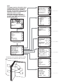


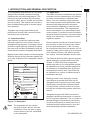
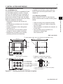
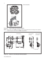
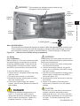
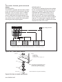
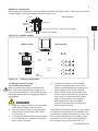
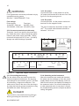
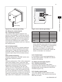
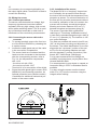
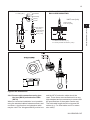
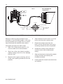
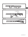
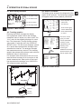
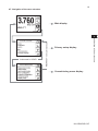
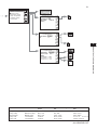
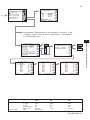
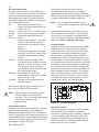
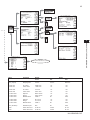
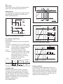
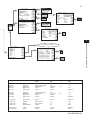
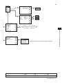
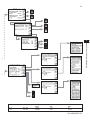
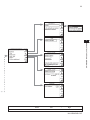
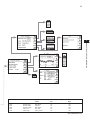
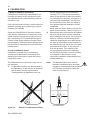
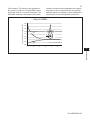

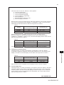
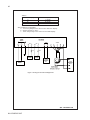
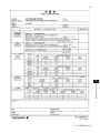

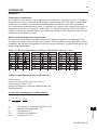
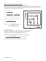
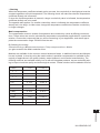
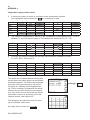
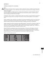
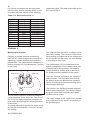
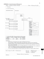

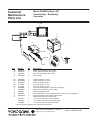
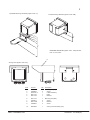
![Model SC450G [Style: S2] Conductivity](http://vs1.manualzilla.com/store/data/005772923_1-d910951678550c5451dfdc47fd4527d0-150x150.png)
![Model ISC450G [Style: S2] Inductive Conductivity](http://vs1.manualzilla.com/store/data/005904832_1-e9e6bdf8409b6fd37a184b6e2701b530-150x150.png)


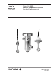

![Model PH450G [Style: S2] pH and ORP Converter](http://vs1.manualzilla.com/store/data/006013412_1-cd77700eed276036ffccc744cbf6fbb4-150x150.png)
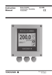
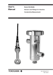
![SS400G MLSS Converter [Style:S2.2]](http://vs1.manualzilla.com/store/data/005726371_1-b873ef07ceb169a0226d293b313a67fd-150x150.png)