1
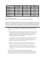
Teaching Improved Methods of Tuning and Adjusting HVAC
Control Systems
Project Introduction
The process control industry has long recognized the importance of control loop tuning. Various
loop tuning methods have existed since the 1940’s and the process industry has been responsible
for a number of advancements in these methods. This includes sophisticated software to
continuously monitor processes and adjust tuning parameters on-the- fly. Such software monitors
all controllers on the local communications bus. The software is designed such that it is also
necessary to know which specific controller models are being monitored. Although complex, it
works well in the process industry where suboptimal tuning can result in significant financial
loss.
However, this does not yet exist in the building HVAC industry for any number of reasons.
First, a common communications protocol for the HVAC control industry has not yet emerged.
It is true the introductions of BacNET and LonWorks have made tremendous strides toward this
goal, but there is a long way to go. There is also the issue of cost. It is unreasonable to assume
building owners will gladly pay substantial monies for software performance monitoring systems
as those currently existing in the process industry. Finally, there is the education component.
Most HVAC control technicians and engineers do not seem to understand the concept of a
formal loop tuning procedure. Persons that are well versed in formal tuning methods often
cannot employ these methods due to any number of restrictions. These restrictions may include
the lack of proper, robust, and inexpensive field equipment and the lack of time to allocate to
loop tuning within the contract in which they are involved.
Thus the goals of this project are actually quite simple.
•
Develop a robust method of data collection in the field independent of the manufacturer
and model of controller found on the job.
•
Keep the cost of such data collection equipment under $1000.
•
Allow the method to be deployed by an educated control technician rather than requiring
the expertise of a control engineer.
•
Develop an instructional learning module for use in the classroom with which to educate
and train the HVAC student in the art of control loop tuning.
Preliminary investigation uncovered an unlikely alternative; the use of a TI calculator and a
handheld data acquisition unit could potentially be used to collect suitable data for a relatively
simple loop tuning analysis.
Project Background
This project has its origin in a previous National Science Foundation (NSF) funded project in
which three control trainers were developed for educating students about Heating, Ventilation,
and Air Conditioning (HVAC) Control. These trainers were used to expose the student to the
steady-state and transient behavior of typical HVAC control systems. These systems were
outfitted with appropriate data recording instrumentation including a flatbed recorder to study
this behavior. As a condition of the project, the results were disseminated via a hands-on
seminar to a group of HVAC professionals. Although impressed with the results, this group
asked the question:
“Could a less expensive and more robust alternative be developed, suitable for
use by engineers and technicians, to check-out and aid in the commissioning of
HVAC systems in the field?”
The commissioning process to which this group referred is a growing trend in the construction
industry. During commissioning, all installed equipment is subjected to a systematic and
rigorous process of checkout, adjustment, and certification. Several issues motivate this trend.
Some of these issues are:
•
The realization on the part of the American worker that they spend an increasing
proportion of their working lives subjected to the interior conditions of the space
including that of indoor air quality
•
The dissatisfaction of tenants and building owners with the performance of installed
systems.
•
An increasing awareness of energy usage and energy costs
Although the control manufacturer is responsible for the competent design of the controller and
associated hardware, it is the designer and the installer that must assume much of the
responsibility for the performance of these systems.
In that vein, HVAC control manufacturers have developed controllers with autotune capability.
However, it is well known autotune has a number of inherent drawbacks. In many cases,
autotune is not invoked due to the processing power required by the feature, thus detracting from
the controller’s primary purpose of controlling the indoor environment. But perhaps more
importantly is the fact autotune is based upon an assumption of linear response. HVAC systems
are predominantly non- linear. Although the process industry has long recognized this, it is
seldom discussed in undergraduate courses or in most HVAC control textbooks. As such, the
typical HVAC control technician is unaware of the existence of such nonlinearities, much less
how to cope with them. As a result, most HVAC control systems are tuned via rule-of-thumb
procedures that do not take into account the unique characteristics of individual systems and
loops.
It is also disconcerting that control manufacturers will often propagate such procedures. If one
were to review the user’s manual for a typical process controller, one would find pages of text
explaining some method of manually tuning the control loop. This is not generally the case with
HVAC controllers. The following is an excerpt from the manual of a well-known HVAC control
manufacturer regarding the adjustment of the integral time constant for a particular family of
controllers.
RESET TIME ADJUSTMENT ([MODEL A AND B] ONLY)
Adjust reset time (Tr), according to the job drawings, with reset time adjustment
knob. Decrease setting until system becomes unstable. Increase setting slightly
until system becomes stable.
It is obvious to the practiced control engineer such instructions do not well serve the end goal of
an optimally tuned control loop. Many instruction manuals that accompany an HVAC controller
do not even address the issue of loop tuning. Thus, a common rule-of-thumb practiced by the
HVAC control technician is to adjust the controller gain until the end device stops moving. The
lack of understanding of integral and derivative control modes usually precludes the use of these
control modes in the typical HVAC loop, even if the loop would be well served by including
these modes. Even if integral control is originally set up during the commissioning process, it is
often disabled shortly thereafter by the building operator. This is generally a direct result of the
lack of understanding of control loop tuning and the inability to properly adjust a loop that has
become unstable.
Further literature review by the authors also uncovered a survey done by Tecmation1 indicating
the following facts about the process control industry:
•
•
•
•
30% of controllers are operated in manual
65% of controllers are poorly tuned or de-tuned to mask control related problems
50% of actuators, transducers and positioners are improperly calibrated
20% of control systems are not properly configured to meet control objectives
Another issue of poorly tuned control loops involves increased valve maintenance. Although
there has been an increase in the application of electronic actuators in the HVAC industry,
pneumatic control valves are still quite common. Valve maintenance in an improperly tuned
loop can become expensive. This topic was addressed by Top Control USA, Inc. in an
April 2002 issue of Control Magazine2 . Their results are summarized below.
•
•
•
Valves are 50% to 75% of system first cost, but as much as 90% of loop maintenance
cost
Valves in a well-tuned loop may stroke 15 to 200 times per day. Poorly tuned valves
may stroke up to 50 times as much
Air typically costs $100/yr/scfm
Not Tuned
Tuned
Savings
Strokes/day
100
20
80
Tuning Cost
$0
$100 - $200
($200)
Maintenance
$1000
$500
$500
Air Use
$480
$100
$380
1x
2 – 5x
Valve MTBF
Savings
$680/valve
(Based on $0.06/kWh)
Table 1: Potential Valve Savings
(Source: Top Control USA, Inc. as printed in Control Magazine, April 2002)1
The aforementioned studies are primarily geared to the process control industry. However, there
is little reason to suspect the HVAC industry is immune to such considerations. For example, the
following is excerpted directly from a report prepared by the Oregon Office of Energy regarding
a case study of the Direct Digital Control (DDC) systems in the Oregon public school system. 3
However, in its work with schools, the Oregon Office of Energy has discovered
that a DDC system sometimes brings a school more problems than benefits. For
example:
•
To maintain stable temperatures in 60 percent of its classrooms, a new middle
school had to manually operate its malfunctioning DDC system. Maintenance
staff members bypassed the $144,000 automated controls to modulate the
supply air temperature. They manually opened the heating valve in the air
handler and adjusted the outside air damper.
•
A new elementary school's $77,500 DDC system caused the building's heating
and ventilation system to run around the clock, even on weekends. The
building's air pressure was so high that doors could not close automatically
and several rooms were always too hot or cold.
•
An elementary school built 20 years ago spent $100,000 on an energy
efficiency retrofit that included new steam actuators, new damper actuators,
T8 lighting, an 80-gallon water heater to replace boiler water heater
operation in the summer, and a DDC system that served only as a glorified
time clock. The result was a utility bill that increased from $11,000 a year to
$17,000 a year.
We estimate that about 200 or one-sixth of Oregon K-12 schools have
dysfunctional DDC systems. By fixing DDC design, installation and user errors,
these schools could save an estimated 11.5 million kWh and nearly one million
therms of natural gas. They would cut their energy costs by a total of more than
$1 million per year. They also would increase building comfort and reduce the
amount of staff time spent on jerry-rigging the DDC and HVAC systems to work
correctly.
It quickly becomes obvious that building control systems require significant attention. It should
be noted the Oregon study does not specifically state nor imply all the problems they experience
are related solely to control loop tuning. However, what is obvious is the lack of understanding
of control systems by a number of those involved. One step toward helping to solve this problem
is to educate and train appropriate individuals on the dynamics of a control loop and how to tune
that control loop for optimum efficiency. To do that, field personnel require a simple,
inexpensive method to collect data so as to perform the proper analysis. It is expected such
analysis will have one of two results:
•
The analysis will result in a set of tuning parameters allowing for proper and optimized
control loop response
•
The analysis will quickly show difficulties in the control loop that are not easily handled
in the field. Such difficulties can be reported back to the design office for proper
dispensation.
Project Approach and Execution
The original NSF grant that spawned this project made use of a laboratory-grade flatbed recorder
to make a record of the dynamics of the control loop studied by the student. This worked well in
the classroom. However, such a device is far too expensive and far too delicate to withstand the
abuse one encounters in the field. When this project began, there was little available in the way
of equipment designed specifically for the proper collection of data in the field for the purpose at
hand. One consideration was the use of a hand- held oscilloscope. However, the cost and
complexity of such a device ruled it out immediately. It quickly became apparent that the TI-83
series of graphing calculators, coupled with a handheld data acquisition unit by Vernier, would
be quite suitable.
The graphing capability of the calculator provided the ability to monitor the dynamics of the
system in real- time. A major advantage was the fact many students already owned a TI
calculator. Also, the Vernier data logger, designed specifically for use in schools, was quite
inexpensive. This means a contractor, a consulting engineer, or even the building owner could
easily purchase the unit since payback would be rapid. Since most technicians already carry
laptop computers, it becomes a simple matter of downloading collected data to the computer for
analysis.
Typical HVAC processes will include temperature control, pressure control and flow control.
Temperature control can be further sub classified into space temperature control and discharge
temperature control. The speed of response of each control loop is substantially different. By far
the slowest loop is space temperature control where the period of cycling may be 20 minutes or
more. The fastest loop is generally the pressure control loop where response can be measured in
seconds. To collect tuning data on such loops requires the equipment have several features.
•
First, the calculator must have significant programming capability to allow for flexibility
in its application. This also means it should be able to be easily reconfigured for cases
not originally considered by this project team.
•
The calculator and the data logger system require significant memory to collect and store
data.
•
The sampling rate of the data logger needs to be sufficiently short to collect enough data
to define the waveform of a fast cycling process such as pressure.
•
The sampling rate of the data logger needs to be sufficiently long to collect data for
something like a temperature process. Since temperature processes are usually not very
noisy and take a long time to cycle, it is unnecessary to collect large amounts of data to
properly define loop oscillations. Coupled with number three above, this means a
variable sample rate is desired.
•
The data logger is required to accept two synchronized inputs. One input is from the
sensor-transmitter for the control variable being analyzed. The second input would have
to record the step signa l used to induce system upset. The inputs would have to be
synchronized in the time-domain to allow loop analysis by any one of a number of
available open- loop tuning methods one might wish to employ. The inputs would have to
be capable of accepting common process signals as found in the HVAC industry.
•
The unit must be able to analyze the data on the spot to provide proper tuning parameters.
Lacking this capability…
•
…the unit must easily interface with a computer to allow downloading data for analysis
•
The calculator and data logger must be able to operate on either batteries or AC power. If
operating on batteries, one must be able to check battery condition to handle situations
where the unit must remain on for several hours.
The TI-83 Silver Edition and Vernier LabPro data logger met all above requirements except the
sixth (the ability to analyze data on the spot). Although the calculator has significant RAM, most
of it is used for data storage only (referred to as archive memory), not for running progr ams.
However, it does have significant data storage capability. As such, we developed this unit to
collect and store data in the field. The data would be downloaded to a laptop at a later time for
proper analysis.
The TI-83 calculator was programmed to control the data logger from the calculator keyboard.
To apply the unit in the field, one input of the data logger is connected to the transmitter used to
send the signal to the controller. The user must also determine the voltage output of this
transmitter over the range the tuning process will occur. The second input of the data logger is
connected to a trigger signal. It is this signal that provides a disturbance to the control loop
while signaling the data logger to begin data collection. This trigger could be a set point change
or a simulated load change.
A set point change may be accomplished in a number of ways. The easiest way to do this is to
establish a reset schedule that will induce a step set point disturbance upon introduction of the
trigger signal. One could also change the set point at the central monitoring station, but the
signal would have to be placed on a spare controller output so it could trigger the data logger to
begin collection.
Instead of a set point change, one could simulate a step load change. To do this, one would place
the controller in manual and move the final control device to some desired position away from
steady-state conditions. Once the system has settled out, the operator would place the controller
back in automatic. The control loop would see this as a step load change and respond
accordingly. Of course, one must also place a trigger signal on a spare output to trigger the start
of data collection when the controller is put back into automatic.
To accommodate either situation, the calculator program provides the user with a series of option
screens. These screens allow the user to adjust parameters for:
•
Data collection rate (sample time)
•
Transmitter voltage range (used to set y-axis limits on calculator graph display)
•
Trigger voltage level
•
An override option to begin data collection without a trigger (useful for closed loop
tuning)
•
The amount of time over which to collect data
•
A battery monitor for the calculator and data logger
•
Plot smoothing (affects display only, not raw data)
•
Data save routines
A typical data plot of an operating system is shown below.
Figure 1: Calculator plots of control system response. The first is a plot
of the raw collected data. The second is a smoothed version of the first.
The third is the response of an untuned oscillatory system.
Once the data is collected, it is easily downloaded to a laptop through TI Connect or
TI GraphLink. The data is imported into an Excel spreadsheet, plotted, and then printed for a
graphic hand analysis. For purposes of this project, we employed the application of the ZieglerNichols closed-loop method, the Ziegler-Nichols process reaction method, and the Cohen-Coon
open loop method. However, one could easily employ other tuning methods as might be
appropriate for the process at hand.
Currently, the method makes use of a graphical technique using hand-calculations. However, the
use of Excel or other program such as MathCAD could be used to further automate the procedure
for use in the field.
Practical Considerations - Hardware
When this project began, the TI calculator and TI CBL (Calculator Based Laboratory) by Vernier
were the only equipment available to meet the criteria outlined above. Soon after, TI dispensed
with the original CBL. Vernier introduced a new CBL and renamed it LabPro. Unfortunately,
Vernier soon learned their products were becoming popular for research, commercial, and
industrial use. This was outside their original intent of education. As such, and part way through
this grant, Vernier began posting a disclaimer on their website and in their product literature
specifically prohibiting such use. To that end, we investigated other options.
The first option was the use of the Casio graphing calculator with their data logger. Due to the
similarity to the TI solution, we did not explicitly test the recent version of the Casio data logger.
However, the use of the calculator and a review of the capabilities of an older data logger proved
the solution to be quite viable. Competitive in price, it has slightly more features and capability
than the TI unit.
For a short period of time, Hewlett Packard and a small company called Firmware Systems
provided a competitive product in the form of the HP-48g and the Firmware Systems Portable
DataLab. Although designed to compete in the educational market, it was also slated for use in
the industrial setting. This system had much greater capability than either Casio or TI;
capabilities approaching that of a handheld computer. Unfortunately, business concerns
rendered the system unavailable, thus we conducted no further investigation into this option.
Technology advancements allowed the introduction of a number of data logging devices. While
most could not meet the requirements outlined above, we did locate one such device, the
MultiLogPro, produced by Fourier Systems, Inc. Under the grant, we purchased several of these
devices and have used them successfully for purposes of HVAC control loop tuning. The
MultiLogPro was originally designed by Fourier to compete with the Casio and TI systems
within the educational market. However, Fourier soon learned the MultiLogPro was also well
received in industry. To that end, they introduced the DAQPro and the TriLog. The TriLog is
essentially the MultiLogPro with wireless data logging capability and no display screen. The
DAQPro is the big brother to the MultiLogPro. The MultiLogPro has four input channels, but
can only accept signals in the 0-10 V or 4-20 mA range. The DAQPro has eight input channels
and will accept virtually any process signal in use today. Competitively priced with the
calculator systems, the MultiLogPro is very intuitive, provides visual real- time graphing of data,
will handle most of the control signals found in the HVAC control industry. Although the
MultiLogPro does come with its own analysis software for installation on a laptop, we found it is
still preferable to download the data from the MultiLogPro to a laptop computer and use Excel to
perform the analysis. For both the educational market and for use in the field, the Fourier
devices have proven quite efficient in allowing us to reach our objective.
Practical Considerations - Field Application
This project was supervised by a group of local HVAC industry engineers involved in HVAC
control. As a group, we firmly believe the outlined process could be implemented within the
HVAC industry and within the HVAC classroom. We also believe it could have great impact on
the industry as a whole in terms of improved comfort and energy savings as the result of
optimized control systems. However, there are a few practical concerns.
The ability to connect the data logger to a control system would require the terminals be
accessible. This could be easily accomplished by wiring the terminals into a terminal block
behind a locked panel. Obviously, this will add additional cost to the project.
An even greater consideration is one of manufacturer warranty. Within the HVAC industry, it is
usually the HVAC control manufacturer or authorized representative that will have a service
contract with the building owner. This brings up the practical issue of warranty considerations.
Although connecting the data logger to a control device is no different than reading the voltage at
that device with a multimeter, our advisory committee felt this issue might prevent widespread
implementation on newly constructed or renovated facilities. However, on systems out of
warranty or where a service contract does not exist, this method is easily applied.
Although the issue of using this method to tune pneumatic systems is not discussed in detail, it is
applicable. To do so, one will need to select appropriate electronic transmitters to install,
temporarily, along side the pneumatic sensor-transmitter units. Of course, the pneumatic units
remain part of the control loop while the electronic units are used only to observe system
response. They are the interface between the pneumatic system and the data logger. The trick is
to use an electronic transmitter with a time constant similar to that of the pneumatic units so they
provide a proper view of system response.
Project Deliverables
A final outcome of this project is learning materials designed to teach the methodology described
above. If desired, one can use the materials as a full course in introductory control, or they can
be used in part to provide instruction and activities regarding control loop tuning using the
methods described above.
The developed materials are currently employed in two control courses at Sinclair Comunity
College. The first course is introductory, thus the developed material starts off by covering the
fundamentals of controllers, valves, sensors, and transducers. This includes the basic operation
and the calibration of these devices. However, the material also covers the more advanced topics
of dead time, time lag, cascade and reset control, and open-loop vs. closed-loop tuning methods.
There is strong emphasis on the time elements of a control loop to allow the student to better
grasp the importance of these elements to the process of loop tuning.
Most elements of the presentation are reinforced with a lab component. The lab component
includes either a computer-based simulation or actual hands-on opportunities. Past presentations
of this course relied heavily on computer-based simulations to perform the loop tuning portion of
the course. However, it became apparent the student was unable to translate the computer screen
to real-world equipment and often left the course unsure of how the course material would apply
to them on the job. By using the methods outlined in this paper, we’ve been able to reinforce the
computer simulations with an actual hands-on task.
In our first control course, the hands-on task is a tuning lab accomplished on a very simple static
pressure control loop using a PI controller. Often, the instructor first demonstrates the lab using
a flatbed pen plotter. This seems to allow the instructor to more easily explain what signals are
being traced, what they represent, and what to do with the trace once you have it.
At this point, the students perform the same analysis using the electronic means of data
collection. With the instructor’s help, they download the data to an Excel spreadsheet, print it,
and then perform a loop analysis by hand. In our case, our goal is quarter-wave damping using
the Zeigler-Nichols method of loop tuning. However, any method may be used as desired. Once
they have the proper values of controller parameters, the students enter those parameters into the
controller and check the results. By repeating the process, the students make a determination if
these parameters need to be tweaked. The students repeat the tuning process to refine the tuning
parameters until the system responds as desired. The students perform this tuning method on
both a proportional controller as well as a proportional- integral controller so as to compare the
two control modes. Of course, a slower responding process, such as temperature control, could
be developed if someone wished to use this method to teach the tuning of a proportional- integralderivative (PID) controller as well.
Our second control course focuses more on control strategy rather than loop tuning and is not
actually part of the grant. However, this course still requires the students to complete a controlloop commissioning project. In this advanced project, the student is presented with a building
economizer system. The system is equipped with variable speed fans and relevant temperatures
are simulated. This system involves three separate but interacting control loops: supply fan
discharge static, return fan tracking based on CFM, and space pressurization. Upon full
calibration of all cont rol devices, development of the control strategy, and the writing of the
controller program, the students are then responsible for properly tuning all three interacting
loops. This allows the student to apply what they learned in their first course to a very realistic
scenario.
The application of these methods within these two courses is fairly recent. However, even if
anecdotal at this time, student understanding and retention of loop tuning methods appears to
have improved tremendously. Educational materials, methods and programs will be available for
dissemination in June 2006.
Project Summary
The purpose of this grant focused on how to teach control loop tuning to the HVAC student and
how to implement a proper tuning process in the HVAC control industry. To the process control
engineer, this procedure is rather trivial. However, the HVAC industry has yet to adopt formal
tuning procedures due to the perceived complexity, lack of knowledge, and lack of time to
perform these procedures.
This project proves that the employment of such methods in the field is quite viable.
Inexpensive equipment is available for data collection and basic loop tuning methods are
relatively easy to learn. By its very nature, the tuning process provides documentation of the
control loop as required by most commissioning contracts. Any loop tuning process has the
advantage of uncovering or identifying control loop problems otherwise difficult to determine.
Thus, the deployment of this methodology would go a long way toward improving building
operations as well as reducing system energy and O&M costs.
Bibliography
1.
Ender, David B, September 1993, “Process Control Performance: Not as Good as you Think ”, Tecmation, Inc.
2.
Buckbee, George, January 2002, “Control Valves: The Hidden Cost of Poor Controller Tuning”, Top Control
USA, Inc.
3.
Churchill, Gregory, 1995, “The Direct Digital Control Crisis in Oregon Public Schools: Offering Solutions
Through Trouble-Shooting Services, Construction Specifications and DDC Circuit Rider Services”, Oregon
Office of Energy
4.
Schaffler, Lawerence, July/August 1998, New Zealand Pine International Magazine, Pg. 21-24