Download Markit 1.04 User Manual & Tutorial Table of Contents

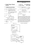
Markit 1.04 User Manual & Tutorial
Latest Update: 10/16/07
Author: Ryan Welch [email protected]
Table of Contents
1.
2.
3.
4.
5.
6.
7.
8.
Why?
Downloading / Installing
Data Preparation
Running Markit
The Nitty Gritty Details
In Practice – Real Usage
Troubleshooting / FAQ
Appendix
A. Building From Source
B. Algorithms
C. Command Line Arguments
D. References
Section 1: Why?
Markit addresses the question: “What variables in my dataset best predict the outcome of interest?”
For a very simple example, consider you have a light bulb that can be either OFF or ON (duh.) Also, on the
wall, we have a set of 4 light switches. You’re not sure which switches are required to turn the bulb ON or OFF,
and even worse, it may be a combination of switches required, not just one. So, you perform a set of
experiments, and end up with the following observations:
OFF
ON
ON
OFF
ON
OFF
UP
DOWN
DOWN
DOWN
UP
UP
DOWN
UP
UP
DOWN
UP
UP
UP
UP
UP
DOWN
UP
DOWN
UP
DOWN
DOWN
UP
DOWN
DOWN
Which light switch turns the bulb on? Or is it actually a combination of switches that turn the bulb on?
And even worse: what happens if there’s a short in the wires from the switches to the bulb? Maybe each time
you flick the switch, even though it should in theory turn the bulb on, the wire shorts and the electricity doesn’t
reach the bulb? Sounds like a tough problem to solve.
This is exactly what Markit attempts to solve using a Bayesian network structure learning methodology. Don’t
worry – if you don’t know what that means, you’re safe.
Section 2: Downloading / Installing
Markit can be built from source, or downloaded as a pre-compiled binary. Additionally, we’re more than happy
to compile it for your specific architecture and operating system if provided with a SSH account on your
machine of interest.
In the future, Markit may be added to a web project known as Bubble.
Binary distributions are available for x86-win32 and ppc64-darwin. If you are not on either of those
platform/architecture combinations, you must build from source. This is as simple as running:
./configure
make
sudo make install
from within the build\unix directory found within the Markit source distribution.
Section 3: Data Preparation
First, we need to cover some unfortunate but necessary ground – how to format your data such that Markit can
use it. Markit supports two formats, but we’ll cover the most important and preferred one here. The format was
originally created by the Orange project, a machine-learning and data mining application and scripting suite
developed by the AILab. Markit actually doesn’t implement the format perfectly, because it only supports a
subset of the features that Orange does.
Let’s continue with our light bulb problem. Our formatted dataset would then look like this (note that we’ve
added a few more observations… we really, really want to know the answer!):
Bulb
discrete
class
ON
OFF
ON
OFF
OFF
OFF
OFF
ON
ON
OFF
OFF
OFF
Switch_1
discrete
Switch_2
discrete
Switch_3
discrete
Switch_4
discrete
UP
UP
UP
DOWN
DOWN
DOWN
DOWN
DOWN
UP
UP
DOWN
UP
UP
DOWN
UP
DOWN
DOWN
DOWN
DOWN
UP
UP
DOWN
DOWN
DOWN
UP
DOWN
UP
DOWN
DOWN
UP
DOWN
UP
UP
UP
DOWN
UP
UP
UP
UP
DOWN
DOWN
UP
DOWN
DOWN
UP
UP
UP
UP
Important note: the dataset should be tab-delimited. It doesn’t look like it above, but that’s just to make it look
prettier for this document. Each column is a variable, and each row is an observation.
The first row specifies the variable names. These can be anything alphanumeric, and can include any character
you’d like. We recommend you avoid spaces as other programs sometimes don’t like them, but if you use
spaces, Markit will take it.
The second row specifies the data type of each variable. Since Markit only works with discrete data, this row
will always contain “discrete” for each variable. You can also use ‘d’ for short.
The third row allows you to specify which variable is the class, or outcome, variable. In our light bulb
experiment, the light bulb’s state (ON/OFF) was the outcome we were interested in.
From here on out, each row contains data. Your data must be discrete, i.e. your variables should have discrete
states like { 0,1,2,3 } or maybe { UP, DOWN }. Anything is game, but you should avoid having too many states
if at all possible.
What about limitations on size of the dataset? Just to give you an idea: this software was designed to run with
genome wide association data, or SNP data for short. These datasets typically have on the order of 2000
observations, and 300,000 variables – and this still only requires approximately 700 MB of RAM. Markit has
also been tested on x86_64 and ppc64, so if you have a 64-bit machine, the sky is the limit.
Section 4: Running Markit
Markit is a command line program. No fancy GUIs, no slick web 2.0 interface, nada. Just you, the shell, and
Markit.
For clarity, let’s define markit as the absolute file path to the markit executable. Wherever you see this,
substitute it with how it exists on your system. On Windows, this could be C:\Documents and
Settings\Desktop\User\markit.exe. On Unix, maybe you’ve placed it in /usr/local/bin/markit. If you’re in the
same directory as the binary, you could simply do ./markit. And if the Markit executable is on your PATH in
either Unix or Windows, it would just be simply ‘markit’.
Let us also define bulb as the absolute file path to the dataset we’ve shown above. Normally this file lives
under <markit root>\data\tests\bulb.tab, but maybe you’ve placed it elsewhere, or created it yourself. That’s
okay.
To get started, let’s try one light switch at a time and see what happens. To do this, run the following command
line:
markit --orange bulb --exhaustive --take_k 1 -s 10
And what do you see?
% Importing data..
% Time required: 0d:0h:0m:0s
% Executing search..
% Time required: 0d:0h:0m:0s
% Writing posterior distribution..
#
0
1
Network
Bulb: Switch_2
Bulb: Switch_3
Score
-25.3844
-29.5904
2
3
Bulb: Switch_1
Bulb: Switch_4
-33.995
-36.4272
Looks rather cryptic, we know. First, let’s explain the command line. Exhaustive means we’re trying every
possible combination of light switches. The “take_k 1” parameter just says we’re looking at 1 switch at a time.
If we changed this to 2 or 3, we would be trying combinations of 2 or 3 switches at a time, exhaustively. The “-s
10” parameter just sets a maximum on how many of the best combinations will be kept, and later displayed, to
you.
Now for the output. The top bit is just console chatter – what the program was doing, and how long it took. For
small datasets, this shouldn’t take too long – almost instantaneous. For larger datasets, you’re looking at
anywhere from minutes to hours (and potentially days, if you get crazy enough.)
The last part is the interesting part – the posterior distribution. Think of this as a sorted list of our best models,
where each model is a combination of light switches (or perhaps just individual switches.) The list is sorted by
score, which in Bayesian language is the natural log of the P(M|D) as computed using the BDe scoring function.
Don’t know what that is? No problem. Just remember these facts:
•
•
•
The score only allows you to compare models with each other, and only when the underlying data is the
same amongst the models you are comparing.
The score is in log units. This means that, in the above example, model #0 is not just about 4 times
better than model #1, it is about 54 times better than model #1.
The larger the score, the better. The numbers are negative, remember – so closer to zero is better.
So now we’ve tried each switch individually, and we have results above. But what if we had tried 2 switches at
a time, or 3? Would those models prove to be better? Well, let’s try it.
markit --orange bulb --exhaustive --take_k 2 -s 10
% Importing data..
% Time required: 0d:0h:0m:0s
% Executing search..
% Time required: 0d:0h:0m:0s
% Writing posterior distribution..
#
0
1
2
3
4
5
Network
Bulb: Switch_2
Bulb: Switch_1
Bulb: Switch_2
Bulb: Switch_1
Bulb: Switch_3
Bulb: Switch_1
Switch_3
Switch_2
Switch_4
Switch_3
Switch_4
Switch_4
Score
-20.7929
-24.1532
-26.4558
-30.5011
-31.1592
-34.6754
markit --orange bulb --exhaustive --take_k 3 -s 10
% Importing data..
% Time required: 0d:0h:0m:0s
% Executing search..
% Time required: 0d:0h:0m:0s
% Writing posterior distribution..
#
0
1
2
3
Network
Bulb: Switch_1
Bulb: Switch_2
Bulb: Switch_1
Bulb: Switch_1
Switch_2
Switch_3
Switch_2
Switch_3
Switch_3
Switch_4
Switch_4
Switch_4
Score
-23.3704
-24.035
-26.2506
-29.8945
Comparing all of our models (remember we can do this, since the underlying data bulb has not changed), it
appears that the score colored in yellow is the best, and drastically better in fact – it is almost 3 natural log units
better than the next best model. Selecting from all of these models, we would put our money on this being the
correct combination of switches to use when attempting to light up that bulb (and in fact, it is, because we
generated our light bulb dataset from a Bayesian network where switches 2 and 3 control the bulb!)
What if you didn’t have a guess as to how many switches it would take? In this running example, we assumed it
would take 1-3 switches to turn on that light (and 3 is ridiculous, but you never know with some engineers.)
There are a few ways to handle this problem.
1. Increase your take_k parameter. Be warned, though – this causes the running time of the program to go
up in a polynomial fashion. So for example, if you have n light switches, the running time will be on the
order of ntake_k. For very large n, you should probably stick around 1-2. For smaller n, you may be able
to get away with 3-5. We recommend starting small, and gradually increasing.
2. Try using --ladder instead of –exhaustive (explained below.)
The ladder method of searching using a heuristic approach to determining which variables to try in combination
with each other. For the previous example, we could have simply done:
markit --orange bulb --ladder --start_k 1 --cutoffs 4,4 -s 10
% Importing data..
% Time required: 0d:0h:0m:0s
% Executing search..
% Time required: 0d:0h:0m:0s
% Writing posterior distribution..
#
0
1
2
3
4
5
6
7
8
9
Network
Bulb: Switch_2
Bulb: Switch_1
Bulb: Switch_2
Bulb: Switch_1
Bulb: Switch_2
Bulb: Switch_1
Bulb: Switch_2
Bulb: Switch_3
Bulb: Switch_1
Bulb: Switch_1
Switch_3
Switch_2 Switch_3
Switch_3 Switch_4
Switch_2
Switch_2 Switch_4
Switch_4
Switch_3 Switch_4
Switch_3
Score
-20.7929
-23.3704
-24.035
-24.1532
-25.3844
-26.2506
-26.4558
-29.5904
-29.8945
-30.5011
What happened? The ladder algorithm here begins with trying 1 switch at a time, as specified by --start_k 1.
It then discovers the best 4 switches (the first 4 in --cutoffs 4,4), and then tries 2-way combinations of those
switches. Finally, it will then try 3-way combinations of the best 4 switches currently known, and write the
results to the output.
Here’s a mockup visual example of what is happening, using more variables. Let’s say we have { A, B, C, D, E,
F, G } as our variables, and we say --start_k 1 and --cutoffs 5,4. Let’s also say we set -s 5, so we’re
only ever keeping 5 of the top best networks (models).
Run 1-way
combinations

Model Score
A
-1.2
B
-1.4
C
-5.3
D
-5.7
E
-6.2
Advance 5 of
the best
variables
Run 2-way
combinations

Model Score
A
-1.2
AB
-1.23
B
-1.4
AC
-2.1
BD
-2.3
Advance 4 of
the best
variables
Run 3-way
combinations

Model Score
A B C -1.0
A
-1.2
AB
-1.23
A B D -1.32
B
-1.4
Does it really make sense to do this with so few switches, or variables? Not really. But it gives you an idea of
how this might work were you faced with a large number of variables. You would start by using --start_k 1
or 2, and then lower your cutoff values as you move forward.
Section 5: Troubleshooting / FAQ
1. Issues involving data.
i. My dataset is formatted where columns are observations, and rows are variables. How do I get it to be
the opposite (to transpose it)?
ii. My dataset has continuous values instead of discrete – is there a way to discretize my data?
2. Issues involving Markit.
i. I’m getting the "The k parameter (number of take-k combinations) must be less than the number of
variables in your data" error message. What does it mean?
3. Issues involving the Unix shell.
i. I want to run Markit for a very long period of time, but I don’t want it to terminate when I close the
terminal window. How do I avoid this?
Appendix
A. Algorithms
More to come on this section soon, including flow diagrams, etc.
B. Command Line Arguments
--orange
Specifies the Orange formatted dataset to use. This must be an absolute path to a file. If you
don’t specify a file, the program should quit. If you specify a file that doesn’t exist, something
bad will probably happen.
--in
Specifies the basic formatted dataset to use. This is an old file format which is deprecated, but
still supported.
--name
The format is simply the Orange format without the 2nd and 3rd lines. Note, though, that without
a class specifier, you’ll have to use the -n argument.
Specifies the project name to be used when creating output files. At a minimum, a file called
<project name>.posterior.tab will be created.
If --maxlike or --density are specified, <project name>.maxlike.tab and <project
name>.density.tab will be created as well.
-s
If --name is not specified, results are written to stdout.
Number of networks to store in the posterior. Memory here is not an issue, the sky is practically
the limit. However, the computational time will go up if you increase this value. Probably should
stick around 1000-2000.
NOTE: For the ladder searcher, the posterior size is important! It uses the posterior to figure
out how many variables to advance at each step. So if your posterior is small (i.e., a small
number of top scoring networks are stored) then very few variables will be found to advance at
each step. You should make this number ideally as large as possible! Try starting around 1000,
and move it up as large as possible. For example, start a series of jobs, with –s varying from
1000 to 10000.
-n
--ladder
The response or classifier node number. Usually 0, but could be anything. This is only necessary
when using --in or -i.
Use ladder search. This is mutually exclusive with --exhaustive.
--start_k
The starting k-combination value to use.
--cutoffs
Specifies how many variables to push forward at each stage. For example, in the above
command line, we have 50000,50000,2000,400,180 and the start_k is 1. This means we’ll
advance 50,000 variables to 2-combinations, 50,000 forward to 3-combinations, 20000 to 4combinations, 400 to 5-combinations, and finally 180 will advance to 6-way combinations. Note
that the number of variables available to push forward is limited by the size of the posterior, see
the –s option for more info.
--exhaustive
Use exhaustive search.
--take_k
The k-combinations value to exhaustively search. Don’t get crazy with this number, usually 3 is
even too large unless your dataset is small (below 2000 variables.)
C. References
Here, I’ll list references to papers which can help understand how Markit works. The order in which they are
listed is not standard, but rather listed in order of importance.
Cooper, G. F. & Herskovits, E. A Bayesian Method for the Induction of Probabilistic Networks from Data.
Mach. Learn. 9, 309-347 (1992).
This paper, while sometimes difficult to find online, is *the* paper for understanding the beginning of Bayesian
network structure learning. It is, however, very difficult reading if you don’t have much of a background in
probability theory.
The most important part of the paper, at least with respect to Markit, would be section 1 and 2. More
specifically, page 316 equation 5. This formula is the scoring function we use when evaluating our models.
Simply set P(Bs) = 1 a priori, and that is exactly what we’re computing. In this equation, we’re assuming a
uniform prior over parameters – if you want Dirichlet priors, see Corollary 1 on page 342. If you don’t know
what that means, you don’t need to worry about it. We wouldn’t lead you astray, we promise.
Also: check out the tree on the top of page 317. It is a great way to think about the Nijk (and therefore Nij)
counts, which gets confusing when you’re just starting to learn it.
Heckerman, D. A Tutorial on Learning With Bayesian Networks. (1995).
http://research.microsoft.com/research/pubs/view.aspx?msr_tr_id=MSR-TR-95-06
Yet another great introduction to Bayesian networks, structure learning, handling missing data, etc. It too
though is somewhat difficult without a background in probability theory, but what isn’t?
We recommend you read the whole thing, at least through section 7. Section 7 also happens to be the most
important for understanding the scoring method. See equation 35 on page 24? It’s just a fancy way of writing
the scoring function from the Cooper paper (corollary 1) listed above using gamma functions.
Pe'er, D. Bayesian Network Analysis of Signaling Networks: A Primer. Sci. STKE 2005, pl4 (2005).
http://stke.sciencemag.org/cgi/content/full/2005/281/pl4
If you made it through the first two papers, you probably won’t need to read this one. It does, however, provide
a good summary of Bayesian methods and goes into some detail about how to apply it to experimental data,
which is what you’ll be doing!
Woolf, P. J., Prudhomme, W., Daheron, L., Daley, G. Q. & Lauffenburger, D. A. Bayesian analysis of
signaling networks governing embryonic stem cell fate decisions. Bioinformatics 21, 741-753 (2005).
Here we’re beginning to deviate from theory theory theory and moving into the applied realm. This paper
shows an actual application of a Bayesian network structure search to a real problem. The main difference
between the approach here, and the approach taken with Markit, is that we’re only searching for the best
parents for a node while in the paper they’re searching for the entire network. However, they have very few
variables, and we can have potentially hundreds of thousands. It’s a very different problem.
Hartemink, A. J. Reverse engineering gene regulatory networks. Nat Biotech 23, 554-555 (2005).
Another applied paper from the people who made Banjo, a *great* tool for searching for Bayesian network
structures. If you’re not interested in finding parents of a variable but rather a network, you should be using
this.