Download Equation Editor Manual

Chapter 2: Getting Started
Notes for Microsoft Equation Editor Users
MathType with Word
The “Using MathType
with Microsoft Word”
section in Chapter 5
contains more useful
information for Equation
Editor users. It
describes the
commands and toolbars
MathType adds to Word
that automate equation
insertion, updating, and
numbering in Word
documents.
Once MathType is installed, it effectively replaces Equation Editor as the
application used for editing equations. However, MathType’s installation
program does not delete the Equation Editor application, but simply registers
itself as the editor for equations you have already created with Equation Editor
(and earlier versions of MathType). If you want to change this behavior or finetune it, see the “Equation Conversion Manager” section below.
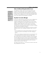
Equation Conversion Manager
Over the years, Design Science has produced several versions of MathType and
has licensed several versions of Equation Editor to many other software
companies, including Microsoft. You may already have one or more of these
installed on your computer now. Every equation is marked with the version of
MathType or Equation Editor that was used to create it. You can see this
information when, for example, you select an equation in a Microsoft Word
document. Word’s status bar near the bottom of the screen will show something
like, “Double-click to Edit MathType 5 Equation”.
MathType Setup automatically registers MathType 5 as the editor for equations
created by all earlier versions of MathType and Equation Editor. This has two
effects:
• When you double-click on an existing equation, MathType 5 will be used to
edit it and the equation will automatically be converted to a MathType 5
equation.
• Other versions of MathType and Equation Editor will no longer appear in the
list of insertable objects in your word processor’s Insert Object dialog.
This is usually what you want to happen, as MathType 5 is more powerful than
those other equation editors. However, if this is not what you want to happen,
you can use MathType’s Equation Conversion Manager to modify this behavior.
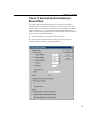
You must exit MathType before running the manager. The Equation Conversion
Manager command is in the MathType 5 submenu, which is located in the
Programs submenu in Windows’ Start menu.
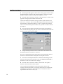
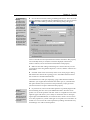
The manager is quite simple to use — if you are not sure what to do, click on the
dialog’s Help button for more details.
9
Chapter 3: Basic Concepts
Chapter 3
Basic Concepts
Introduction
This chapter outlines the basic concepts used in MathType. If you are an
experienced Windows user, you will be familiar with some of them already,
since they are common to many Windows applications. On the other hand, the
symbol and template ideas are unique to MathType, so you may want to read a
little about them.
The basic purpose of MathType is to allow you to create and edit mathematical
equations. In this manual, we use the term “equation” to refer to any
combination of mathematical symbols. The approach to equation creation is very
intuitive and visually oriented. For each basic mathematical construct, like a
fraction or an integral, MathType provides a template containing various
symbols and empty slots. You build equations simply by inserting templates and
then filling in their slots. Chapter 4 explains the techniques in detail.
You will generally be placing MathType equations into a document you’re
creating with a word processor (or a page layout application, or a similar
program). You’ll want to run MathType and your word processor
simultaneously, and transfer equations into and out of your document. Chapter 5
explains several ways to do this.
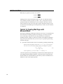
You can start MathType by clicking on the Start button, choosing Programs,
selecting the MathType 5 menu, and then choosing MathType. An empty
MathType window will appear.
11
MathType User Manual
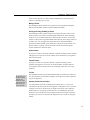
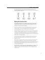
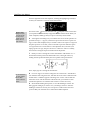
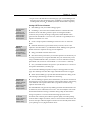
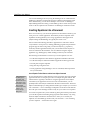
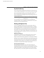
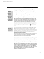
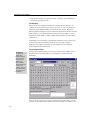
The MathType Window
The picture below shows MathType with all parts of its toolbar visible:
Symbol palettes
Handle
Template palettes
Small bar
Tabs
Large tabbed bar
Palette
Small tabbed bar
Ruler
Empty slot
Insertion point
Selection
Status bar
Within the equation area itself, there are four items of interest:
Empty Slot
A slot containing no text is displayed with a dotted outline.
Insertion Point
A blinking marker consisting of a horizontal line and a vertical line that indicates
where text or templates will be inserted next.
Selection
The part of the equation that will be affected by any subsequent editing
commands is highlighted.
Status Bar
The Status Bar contains four areas that tell you your current settings for Style,
Size, Zoom, and Color. You can change these settings using menu commands or
simply right-click on an area to show a menu for that setting. While moving the
mouse in the toolbar or in the menus, the four Status Bar entries are temporarily
replaced by a message that describes the item the mouse pointer is over. At other
12
Chapter 3: Basic Concepts
times, the message tells you what operation MathType has just performed or
what it is expecting you to do next.
MathType Toolbar
The MathType toolbar contains five separate areas: the Symbol and Template
Palettes, the Small Bar, and the Large and Small Tabbed Bars.
Docking and Floating the MathType Toolbar
The MathType window picture on the previous page shows the toolbar in the
docked position. You can also dock the toolbar at the bottom of the MathType
window or you can make it float above all the equation windows. To move the
toolbar, use the mouse to grab the Handle at the left end, and to drag it wherever
you like. Also, you can toggle the toolbar between its docked and floating
positions by double-clicking on its handle, any unused part of the toolbar, or its
title bar when it’s floating. You can also hide or show the toolbar using the
Toolbar command on the View menu.
Symbol Palettes
If you press or click on one of these buttons, a palette containing various symbols
will appear. If you choose one of the symbols, it will be added to your equation
at the insertion point.
Template Palettes
If you press or click on one of these buttons, a palette containing various
templates will appear. If you choose one of the templates, it will be added to
your equation at the insertion point or, if something is selected, it will “wrap”
around it.
The Bars
Organizing Tip
The Tabs allow you to
organize your symbols,
expressions, and
templates into named
collections. Tutorial 5 in
Chapter 4 shows you
how to rename Tabs.
The Small Bar and the Large and Small Tabbed Bars are containers in which you
can store frequently used symbols, templates, and expressions (whole equations
or parts of equations).
Adjusting Toolbar Size and Content
You will probably not need all of the items described above, so we provide
commands on the View menu for showing them or hiding them as you wish. For
example, if you have a small screen, you might want to keep some of the bars
hidden while you are typing. You can then use one of MathType’s keyboard
shortcuts to show the bar you need, and then use the shortcut again to hide the
bar when you’re done. See Tutorial 5 in Chapter 4 for more advice on using the
toolbar.
13
MathType User Manual
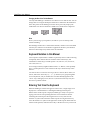
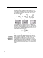
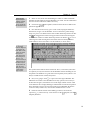
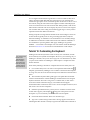
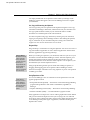
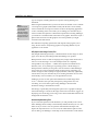
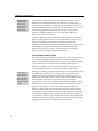
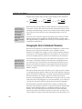
Changing the Size of the Toolbar Buttons
You may find MathType’s default size of toolbar icons too small to read. You can
change their size using the Workspace Preferences command on the Preferences
menu. The picture of the MathType window shown previously displays the
small button size. Here are the three available sizes of buttons for comparison:
Small
Medium
Large
Ruler
Shows you how large your equation is, and allows you to set tab stops that
control formatting.
The MathType window also contains other elements, which we have not labeled
since they are common to most Windows applications. Refer to your Windows
manual or online Help if any of these items are unfamiliar.
Keyboard Notation in this Manual
Your computer’s keyboard has a number of special keys that we will be referring
to frequently in this manual. We will write the names of these keys (and
combinations of these keys) in small capitals: CTRL, SHIFT+A, ALT, BACKSPACE,
CTRL+TAB, and so on.
Your carriage return key might be labeled “Enter” or “Return”, and it probably
has a ↵ symbol printed on it. We will refer to this key as the ENTER key in this
manual.
You will also have a set of four arrow keys: the LEFT ARROW, RIGHT ARROW, UP
ARROW, and DOWN ARROW keys (←, →, ↑, ↓). These keys are grouped together
on most keyboards, and you should have no trouble identifying them as the
“arrow” keys, although your TAB, BACKSPACE, ENTER and SHIFT keys may also
have arrows printed on them.
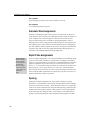
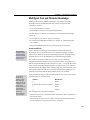
Entering Text from the Keyboard
When the MathType window first appears on the screen, a single empty slot is
displayed as a small dotted box containing the blinking insertion point.
Whenever the insertion point is displayed, MathType is ready to accept text.
Typing will cause the corresponding characters to be inserted into the slot
containing the insertion point. Pressing the BACKSPACE key will erase the
character or symbol to the left of the insertion point. Pressing the DELETE key
erases the character or symbol to the right of the insertion point. When items are
selected in the equation, either the DELETE key or the BACKSPACE key can be used
14
Chapter 3: Basic Concepts
to delete the selection. Pressing the ENTER key will start a new line below the
original line. Immediately after typing, you can choose the Undo Typing
command on the Edit menu to erase everything that you typed since the last
non-typing operation.
Why the Spacebar Doesn’t Work
The SPACE key usually has no effect, since MathType performs spacing of
mathematical equations automatically. Professional-quality mathematical
formatting involves six different space widths, none of which is the same width
as the space character in most fonts, so it would be undesirable to insert the
standard space character into your equations. Many people find this a bit
confusing at first, but you will get used to it quickly. However, sometimes you
might want to insert a non-mathematical phrase into your equations and, here,
the standard space is exactly what you want. To do this, just change the current
style to Text and start typing. See Tutorial 4 in Chapter 4 for details.
Sometimes you may find it necessary to override MathType’s automatic spacing.
There are CTRL (Control) key shortcuts for entering various widths of space; for
instance, CTRL+SPACE inserts a thin space. See Tutorial 6 in Chapter 4 for more
information.
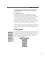
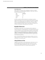
Inserting Symbols
Keyboard Shortcuts
MathType also provides
keyboard shortcuts for
inserting almost all
symbols on the palettes.
These are shown in the
Status Bar when the
mouse is over each
symbol. You can also
assign your own
keyboard shortcut to any
symbol. See Tutorial 16
in Chapter 4 for more
information.
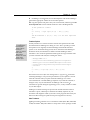
To insert a symbol, you click on it in one of the bars, or choose it from one of the
Symbol Palettes, as shown in the picture below. The Symbol Palettes work like
standard Windows menus — just press or click the left mouse button to display
the palette’s contents, then choose the desired symbol. The symbol will be
inserted immediately to the right of the insertion point or, if something is
selected, the symbol will replace it.
15
MathType User Manual
Inserting Templates
Keyboard Shortcuts
MathType also provides
keyboard shortcuts for
inserting almost all
templates. These are
shown in the Status Bar
when the mouse is over
each template. You can
also assign your own
keyboard shortcut to any
template. See
Tutorial 16 in Chapter 4
for more information.
To insert a template, you click on it in one of the bars, or choose it from one of
the Template Palettes. The Template Palettes work like standard Windows
menus — just press or click the left mouse button to display the palette’s
contents, then choose the desired template. The template will be inserted
immediately to the right of the insertion point or, if something is selected, the
template will “wrap” itself around it.
A template is a formatted collection of symbols and empty slots. You build
expressions by inserting templates and then filling in their slots. You can insert
templates into the slots of other templates, so complex hierarchical formulas can
be built up in a natural way. Slots are “intelligent” in the sense that they control
the properties of any characters inserted into them. For example, any text that
you insert into the upper limit slot in a summation template is automatically
reduced in size and is centered above the summation sign.
Placing the Insertion Point
Equation Structure
To better understand the
structure of your
equation, cycle the
insertion point through
the slots, and watch how
its size and shape
changes. Alternatively,
use the Show Nesting
command on the View
menu. See Tutorial 1 in
Chapter 4 for an
example.
You can place the insertion point within the text in any slot by positioning the
mouse pointer over the desired position, and clicking, just like in a word
processor. Pressing the TAB key or the INSERT key will move the insertion point to
the end of the next slot in the equation. Therefore, by repeatedly pressing the TAB
or INSERT key, you can make the insertion point cycle through every slot in the
equation. (Since the TAB key is used to cycle the insertion point, you may be
wondering how to enter tab characters. This is done with CTRL+TAB.)
If you hold down the SHIFT key while pressing the TAB key, the insertion point
will move around the equation in the reverse direction. You can also move the
insertion point by using the arrow keys; this is described in more detail in the
following section.
You can tell which slot contains the insertion point from its size and shape. The
horizontal line of the insertion point runs along the bottom edge of the slot, and
the vertical line of the insertion point runs from the top to the bottom of the slot.
If you’ve turned on nesting with the Show Nesting command, you can tell which
slot contains the insertion point by its background color.
16
Chapter 3: Basic Concepts
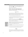
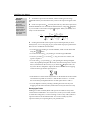
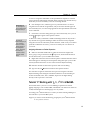
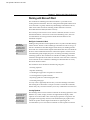
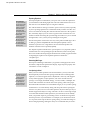
The equations in the first row below show four different insertion point
positions, and the four pictures in the second row show the result of typing an m
into the expression in each case:
Moving the Insertion Point
As described previously, you can use the TAB key to move the insertion point
through all of an equation’s slots. Holding down the SHIFT key moves the
insertion point in the reverse direction. You can also use the arrow keys for
moving the insertion point more precisely.
The rules for using the arrow keys are somewhat tedious to describe (and to
read, no doubt) — it’s easier to experiment with a couple of equations to
understand the behavior. Here’s a quick guide to how they work.
Roughly speaking, pressing the LEFT ARROW key moves the insertion point one
character to the left, and RIGHT ARROW moves one character to the right. If the
next character is a template, the insertion point moves into the template’s first
slot. If there are no more characters in a template slot to move over, the insertion
point will move out of the template.
If you hold down the CTRL+SHIFT key combination while pressing the arrow
keys, the insertion point will move over templates; it will not move into a
template’s first slot.
The UP ARROW and DOWN ARROW keys move the insertion point up and down
between lines or template slots. The up and down directions are generally
determined by the physical location of each slot, but when templates are nested
within templates, the template hierarchy may take precedence, and not every
slot may be passed through.
The HOME key moves the insertion point to the beginning of the current slot, the
END key moves it to the end. The PAGE UP and PAGE DOWN keys scroll the
MathType window up and down respectively, but do not actually move the
insertion point.
17
Chapter 4: Tutorials
Chapter 4
Tutorials
Before You Start
This chapter contains several tutorial examples of using MathType. We provide
step-by-step instructions for each example, so you should find it easy to work
through them. Each tutorial should take you no more than 10 minutes, and they
are by far the best way to learn MathType. Before you start, however, there are a
few things to bear in mind.
First, recall that you can find symbols and templates either in the palettes at the
very top of the MathType window, or in the bars lower down. You have to pull
down the palettes to find the items you need, but you can just click on the ones
in the bars. For the most part, the tutorials will require very common symbols
and templates that we placed in the bars for you before we shipped MathType.
You can change the contents of these bars at any time; we explain how in
Tutorial 5.
Undo and Redo
You can also correct
mistakes by using the
Undo command on
MathType’s Edit menu.
In MathType 5 you can
Undo and Redo an
unlimited number of
times.
Also, you do not have to worry about making mistakes. If you type something
wrong, or choose the wrong symbol from one of the palettes, you can correct
your mistake by pressing the BACKSPACE key.
Fonts and the Appearance of Your Equations
The tutorials will often tell you that “your equation should now look like this.”
In fact, the appearance of your equation will be determined by the fonts you are
using, so you shouldn’t take this statement too literally. MathType’s default fonts
are Times New Roman, Symbol and MT Extra. These fonts will probably be
acceptable, at least for the purposes of working through the tutorial, and we
recommend that you stick with them until you’ve gained some experience
working with MathType.
For the time being, please do not change fonts by using the Other command on
the Style menu — as you’ll see in Tutorial 8, there’s a much better way of doing
this in MathType, and we don’t want you to get into any bad habits.
Some Final Advice
In the first few tutorial examples, we’re going to assume that you’re using
MathType along with Microsoft Word to create a document. MathType works
with a wide variety of word processing, publishing, Web editing and graphics
programs, but Word is by far its most common companion. If you want to work
through the tutorials using some other word processing application, it should be
easy to adapt the instructions that follow. Also, detailed instructions for using
MathType with other applications are available in Chapter 5.
21
MathType User Manual
In the tutorials, we’ll often tell you to type certain characters into your equations.
The characters you have to type will be shown in bold type.
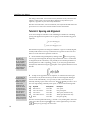
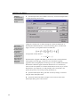
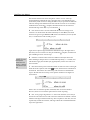
Tutorial 1: Fractions and Square Roots
In our first tutorial, we will create the equation
y=
3
16
sin x − c 2 ± µ tan x
This is a very simple equation, but you’ll learn about fractions and square root
templates, and we’ll explore the properties of the insertion point, and illustrate
MathType’s function recognition and automatic spacing capabilities.
To create the equation, just follow the steps listed below. Remember that the
characters you have to type into the equation are shown in bold type.
1. Open a new Word document, and type a few lines of text, just to make the
situation a bit more realistic.
Word Toolbar
You can insert a display
equation using the
button on Word’s
MathType toolbar. You
can see what each
toolbar button does by
holding the mouse
pointer over the button
for a couple of seconds.
A tooltip will appear
containing the name of
the button’s command.
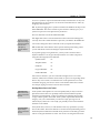
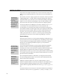
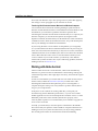
2. Now we’re ready to insert a MathType equation. If you installed MathType
correctly, there should be a MathType menu towards the right-hand end of the
Word menu bar, as shown below.
From the MathType menu choose the Insert Display Equation command. This
will open a MathType window, ready for you to start creating the equation. If for
some reason neither the MathType menu nor the MathType toolbar is available
in Word, use Word’s Insert Object command (choose Object on the Insert menu),
and choose MathType 5.0 Equation from the list of object types displayed. See
Chapter 5 to learn about other ways to insert an equation, either in Word or
other applications.
3. In the MathType window, type y=. You don’t have to type a space between
the y and the =, because MathType takes care of the spacing automatically. To
help you break the habit of typing spaces, the spacebar is disabled most of the
22
MathType User Manual
Selecting Items in an Equation
Selecting Entire Slots
You can select an entire
slot by double-clicking
anywhere in the slot.
This is analogous to the
way many word
processors allow you to
select a word by doubleclicking on it.
As usual in Windows applications, you have to select the items that you want to
operate upon before you choose the command that is to be applied to them. In
MathType, the selected part of the equation will be affected by a subsequent
editing command such as Cut, Copy, or Nudge. To select part of an equation,
you position the mouse pointer over one end of the items to be selected, and then
press and hold down the left mouse button while dragging the pointer over the
equation. The selected items will be highlighted.
Selecting with the Arrow Keys
You can make a selection (or extend a previous selection) by holding down the
SHIFT key and pressing the LEFT ARROW or RIGHT ARROW key. Pressing the arrow
key moves the insertion point through your equation, in the usual way, and
holding down the SHIFT key will cause it to select all the items it passes through.
Selecting Embellishments and Parts of Templates
Holding down the CTRL key allows you to select a character embellishment, such
as a “hat” or overbar, or an item that is part of a template (as opposed to an item
within one of the slots in a template), such as the Σ in the picture below. If you
hold down the CTRL key, then the mouse pointer changes from an angled arrow
into a vertical one. You can then select the template component by clicking on it
with the vertical pointer. This is useful if you want to change the size of a
summation sign or nudge a prime to a new position, for example.
The ENTER Key
Aligning Lines in Piles
You can align the lines
in a pile in various ways
using the commands on
the Format menu.
18
Pressing the ENTER (↵) key will create a new line with a single empty slot
immediately beneath the slot containing the insertion point. A series of lines
created in this way, one above another, is called a pile. You can use piles to
represent matrices and column vectors, if you prefer them to MathType’s built-in
matrices. Pressing the BACKSPACE key with the insertion point at the beginning of
a line will join it back to the line above.
Chapter 4: Tutorials
time in MathType, so pressing it will have no effect (other than producing an
annoying beep!). Chapter 7 discusses where and how you should enter spaces in
MathType, but you won’t have to do this very often.
Also, notice that the y has been made italic, but the = sign has not. Mathematical
variables are almost always printed in italics, so this is the default in MathType.
You can change this by redefining the Variable style using the Define command
on MathType’s Style menu. See Chapter 7 for details.
4. Now we need to enter a square root sign. To do this, click on the
icon in
template’s home is in the
palette, but we’ve also
the Small Bar. The
moved it into the Small Bar to make it easier for you to find. Your equation
should now look like this:
The characters in the equation might be larger than you expect, but this is just a
result of the viewing scale you’re using. You can use the commands on the View
menu to change the viewing scale to anything between 25% and 800%. The
blinking insertion point should be in the slot under the square root sign,
indicating that whatever you enter next will appear there.
Fraction Template
As you hold the mouse
pointer over the palette
items their name is
displayed in the status
bar at the bottom of the
MathType window. This
will help you make sure
you pick the correct
template.
palette and
template — it’s the one on the right in the top row. This template
choose the
produces reduced-size fractions, sometimes known as “case” fractions in the
typesetting world. Case fractions are generally used to save space when the
numerator and denominator of the fraction are just plain numbers. Be careful not
template — this would create a full-size fraction, which
to choose the larger
would be too big for this situation. Notice how MathType automatically expands
the size of the square root sign to accommodate the fraction. Your equation
should now look like this:
5. Next, we enter a fraction template. To do this, go to the
The insertion point should be in the numerator (upper) slot of the fraction
template.
6. To enter the numerator of the fraction, just type 3.
7. Now we need to move the insertion point down into the denominator slot of
the fraction. You can do this by pressing the TAB key or by clicking inside the
denominator slot in your equation.
8. Enter the denominator by typing 16.
9. Next we need to add the sin x outside of the square root sign, and to do this
we have to get the insertion point into the correct position in the hierarchy of
slots that make up the equation. If you repeatedly press the TAB key, you can
23
MathType User Manual
make the insertion point cycle through all the slots in the formula. If you hold
down the SHIFT key while you do this, the insertion point will cycle through the
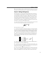
slots in the reverse direction. Try this out to see how it works. Three of the
positions that the insertion point will assume during the course of this cycling
are shown below. Use a viewing scale of 400% or 800%, so that you can see
what’s happening a little better:
If you use the Show Nesting command on the View menu, you can get an even
better picture of the hierarchical arrangement of slots in your equation:
We have to decide which of these insertion point positions is the right one for
adding the sin x. The position on the left is clearly wrong — we don’t want the
sin x to go in the denominator of the fraction. In the position shown in the center,
the insertion point is in the main slot under the square root sign, so if we type in
sin x the result will be the following formula:
This is not what we want either. The insertion point position shown on the far
right is the correct one; the insertion point is outside the square root, which is
where we want the sin x to go.
Functions
You can customize the
list of functions that
MathType automatically
recognizes. Tutorial 4
contains an example.
24
10. Keep pressing the Tab key until the insertion point arrives in the correct
position, and then type in the letters sinx. Type slowly, so that you can watch
what happens. When you initially type them, the s and the i will be italic,
because MathType assumes that they are variables. However, as soon as you
type the n, MathType recognizes that sin is an abbreviation for the sine function.
Following standard typesetting rules, MathType uses plain Roman (non-italic)
format for the sin, and inserts a thin space (one sixth of an em) between the sin
and the x.
Chapter 4: Tutorials
11. Type –c. Remember you don’t have to type the spaces. You insert the minus
sign by pressing the − (minus/hyphen) key on your keyboard. In a word
processor, pressing this key inserts a hyphen, which is typically shorter than a
minus sign. However, since hyphens are very uncommon in mathematics,
MathType replaces them by minus signs for you (when the Math style is in
effect). Your equation should now look like this:
Keyboard Shortcuts
You can also create a
superscript slot by
typing CTRL+H. CTRL+L
inserts a subscript slot.
12. Next we need to attach the superscript (or exponent) to the c. To do this,
click on the icon in the Small Bar. This will create a superscript slot next to the
c, as shown below:
13. Type 2, and then press TAB to move the insertion point out of the superscript
slot, into the position shown below:
14. Click on the ± in the Small Bar. MathType knows that the ± symbol is
supposed to have spaces around it in this situation, so, as usual, you don’t have
to type them.
Greek Characters
You can enter a Greek
character using CTRL+G
and its eqivalent, e.g. m
for µ, P for Π.
palette — it’s the second one from the right in
15. Choose the µ from the
the row of Symbol Palettes. Alternatively, as the Greek letter µ corresponds to
the letter m, you can press CTRL+G, followed by m. Your equation should look
like this:
16. Finish the formula by typing tanx. Again, notice that MathType uses plain
(instead of italic) type for the tan function and puts thin spaces on either side of
it. Your finished equation should look like this:
Keyboard Shortcut
The quickest way to
close the MathType
window is by pressing
CTRL+F4.
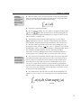
17. Close the MathType window, either by clicking on its close box or by
choosing the Close and return to <document> command on the File menu, and
choose Yes in response to the dialog that asks if you want to save changes. This
will insert your equation into the Word document in “displayed” form (on a line
by itself), like this
y=
3
16
sin x − c 2 ± µ tan x
25
MathType User Manual
18. In other situations, you might want to embed an equation within a line of
text, for example y = 163 sin x − c2 ± µ tan x , rather than displaying it on a line by
itself. To do this, use the Insert Inline Equation command from Word’s
MathType menu or MathType toolbar.
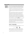
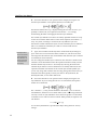
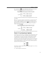
Tutorial 2: Sums, Subscripts & Superscripts
In this tutorial we’ll create the formula that is often used to calculate a statistical
quantity known as variance. The formula is:
1 n
n  i =1

σ X2 = ∑ X i2 − nX 2 

This formula illustrates the use of subscripts, superscripts, and summation
templates. Integral and product templates behave much the same as summation
templates, so what you learn in this tutorial will be useful in a variety of other
situations. The steps required to create the formula are as follows:
1. Open a new Word document, and type a few lines of text.
2. Choose the Insert Display Equation command from Word’s MathType menu
or MathType toolbar. This will open a MathType window, ready for you to start
creating the equation.
3. Enter a σ. One way to do this is to choose it from the
palette.
Alternatively, you could use its keyboard shortcut. The keyboard shortcuts for
toolbar items are displayed in the status bar as you move the mouse over them.
In this case you can press CTRL+G followed by s.
Zoom Levels
A quick way to change
zoom level is to rightclick in the Zoom panel
on the status bar.
Or, you can type:
CTRL+1 for 100%,
CTRL+2 for 200%,
CTRL+4 for 400%, or
CTRL+8 for 800%.
4. Next, create slots for the subscript and superscript on the σ by clicking on
the
icon in the Small Bar. Subscripts and superscripts are rather small. In
order to better see what’s happening, make sure you’ve chosen at least 200%
viewing scale in the Zoom submenu of the View menu.
5. The insertion point will be located in the newly created subscript slot. Type
the subscript, X.
6. Move the insertion point up into the superscript slot either by clicking in it
or by pressing the TAB key. Then type the number 2 into the superscript slot.
7. Now let’s move the insertion point to the location shown below:
Either press the TAB key, or click somewhere out to the right of the equation, as
shown in the picture. Be careful not to place the pointer too close to the subscript
or superscript slots, or else the insertion point may jump into one of them when
you click.
26
Chapter 4: Tutorials
8. Type in the = sign. Remember not to type any spaces.
Inserting Fractions
You can also insert the
fraction template by
pressing CTRL+F.
9. Construct the fraction by using the full-size template, which is available
palette. Be careful — it’s not the same
in the Small Bar and in the
template as the fraction template that we used in Tutorial 1.
10. The insertion point will be located in the newly created numerator slot; type
the number 1 into this slot.
11. Move the insertion point down into the denominator slot either by clicking
in it or by pressing the TAB key. Then type in the denominator, n, and press the
TAB key again to move the insertion point out of the denominator slot. Your
equation should now look like this:
12. Next we need to insert a pair of braces (curly brackets). You can do this
either by clicking on the
icon in the palette, or by using the CTRL+{ keyboard
shortcut. Remember that { is a shifted character on standard keyboards, so you’ll
actually need to hold down the CTRL and SHIFT keys while pressing the key that
bears the [ and { characters.
13. Click on the
icon to enter a summation template inside the braces. Notice
how the braces expand automatically. Your equation should now look like this:
14. Type the letter X into the summand slot (the large slot on the right).
15. Attach a subscript and superscript to the X, using the
template. Fill in the
subscript and superscript slots with i and 2, respectively.
Spacing
Chapter 7 includes a
discussion of
MathType’s spacing
rules and how you can
customize them.
16. Move the insertion point into the lower limit slot of the summation template
by clicking inside the slot, and type i=1. As usual, do not type any spaces.
MathType will automatically reduce the size of the text, and will center it below
the summation sign. In this case, MathType will not insert any spaces around the
= sign, since it is in the limit of a summation. Again, this is a standard
typesetting convention that you can override if you want to.
17. Click in the upper limit slot of the summation template, and type in the
upper limit, n.
27
MathType User Manual
18. Move the insertion point into the position shown below:
If the insertion point is in the upper limit slot of the summation template,
pressing the TAB key will do the trick. In fact, as we saw in Tutorial 1, if you keep
pressing the TAB key, the insertion point will cycle through all the slots in the
equation and will eventually reach the position shown, regardless of where it
started out. If you want to move the insertion point by clicking, click somewhere
near the point indicated by the arrow in the picture above. You might want to
use the Show Nesting command on the View menu to make this easier.
19. Type –nX.
20. Place a bar over the X by clicking on the icon in the
palette. In
MathType, embellishments of this type are always added to the character to the
left of the insertion point. You can even add several embellishments to the same
character. For more details, look for Embellishments in MathType’s online help.
21. Enter the superscript 2 by using the
template. It works just the same way
template that we used earlier. The equation is now complete (well,
as the
maybe it is — see the next step below).
22. We hope you’re happy with the way MathType formats your equation, but,
if you’re not, we’ve provided a way for you to make some fine adjustments of
your own. You can select any item or group of items, in the usual way, and
nudge them either horizontally or vertically in steps of one pixel (screen dot). If
you view your equation at 800% scale you can make adjustments as small as an
eighth of a point.
To nudge items, use the following keystrokes:
CTRL+←
CTRL+↑
CTRL+→
CTRL+↓
Selecting an
Embellishment
You can select an
embellishment by
holding down the CTRL
key and then clicking on
the embellishment.
28
nudges the selected items to the left by one pixel
nudges the selected items upward by one pixel
nudges the selected items to the right by one pixel
nudges the selected items downward by one pixel
You might want to try moving a subscript or a superscript, moving the limits of
the summation, or even moving the bar embellishment.
Keep in mind, however, that nudging is really intended for making small
adjustments that cannot be achieved otherwise. The preferred method for
adjusting spacing is using the Define Spacing dialog, described in Chapter 7.
This approach has the advantage that the spacing rules you define affect all
equations.
Chapter 4: Tutorials
23. Close the MathType window, which will insert the equation into your Word
document. Save the document, because we’re going to use it in the next tutorial.
Tutorial 3: Editing Old Equations
This tutorial teaches you some special editing techniques that are useful when
you’re modifying an existing equation. You will often need to correct a mistake
in an old equation, or make a new one that is a slight variation of one that you
have made in the past. Instead of starting from scratch, you can bring a copy of
the old equation back into MathType and modify it as needed. In this way, all
your old documents serve as sources of material for new documents. You can
store commonly used equations (or fragments of equations) in word processing
documents or as expressions within MathType itself.
Let’s suppose that the equation we created in Tutorial 2 is the wrong one, and we
want to use the following related formula in our document instead:
sX =
1  n 2
2
∑ X i − nX 
n − 1  i =1

The steps required are as follows:
1. Open the Word document containing the equation you created in Tutorial 2
above. We want to bring this equation back into MathType for editing. There are
several ways to do this, as explained in Chapter 5, but the simplest is to doubleclick on it. This will open the equation for editing, in a new MathType window.
2. Select the term on the left-hand side of the equation by dragging the arrow
pointer across it while holding down the left mouse button. The selected items
will be highlighted by black-white reversal, in the usual Windows manner. It
should look like this:
3. Delete the selected items by using the Clear command on the Edit menu, or
by pressing the BACKSPACE key or the DELETE key.
4. The insertion point is in the right place, immediately to the left of the = sign,
so you can now enter the new left-hand side. Type in the letter s and attach the X
template, in the usual way.
subscript to it by using the
5. Next, we’re going to enclose the right-hand side in a square root sign. We’re
template around the existing terms — previously we have
going to “wrap” a
always inserted templates first, and then filled in their slots afterwards. Select
29
MathType User Manual
the entire right-hand side of the equation, watching the highlighting carefully to
see that your selection is correct. It should look like this:
MathType 3 Users
MathType 3 required
you to hold down the
CTRL key to wrap a
template around the
selection. This is no
longer necessary.
icon in the Small Bar. The
template will be inserted into
Now click on the
your equation and automatically wrapped around the selected items. When you
insert a template, MathType always wraps it around any selected items.
6. You might be wondering how you would do the reverse of the operation we
performed in step 5 — suppose you had an expression enclosed in a square root
sign (or some other template) and you wanted to remove the square root sign but
keep the expression. To do this, you first select the expression under the square
root sign and choose Cut to transfer it to the Clipboard. Next, select the (now
empty) square root sign, and press BACKSPACE or DELETE to remove it. Finally,
choose Paste to bring the expression back from the Clipboard.
7. Finally, we have to change the n in the denominator of the fraction to n – 1.
Position the insertion point in the denominator slot, to the right of the n, by
clicking near the point indicated by the arrow pointer in the picture below:
Then, simply type –1 to change the denominator.
Color
You can customize the
Color menu using the
Edit Color Menu
command in the Color
submenu.
8. Let’s now suppose we want to change the color of the term sX from black to
red. Select the term using the mouse, and then choose the Color command on the
Format menu. A submenu appears containing a list of colors. Choose Red and
release the mouse. The selected term will become red (you will have to click
outside the equation to de-select the term in order to see the new color).
9. We’re finished editing the equation, so close the MathType window. If a
dialog appears asking if you want to save your changes, click Yes. Once the
MathType window has closed, your word processor will become active and
you’ll see that your document now contains the modified equation.
30
Chapter 4: Tutorials
Tutorial 4: Including Text in an Equation
In our next tutorial, we show you how to enter words and phrases in an
equation, and also how to handle function name abbreviations that MathType
does not recognize. We are going to create the following equation:
Prob( A | B) =
Prob( A ∩ B)
Probability that both A and B occur
=
Prob( B)
Probability that B occurs
1. First, open a new MathType window using one of the methods you’ve
already learned. Then type Prob(A|B). The result will be
Controlling Italics
To assign regular (nonitalic) style to function
names, use Function on
the Style menu, rather
than just removing the
italics.
Using its built-in table of function names, MathType has recognized Pr as an
abbreviation for “probability” and set it in the Function style, while o and b are
regarded as variables. In this tutorial, we want to use Prob, rather than just Pr, as
our abbreviation for “probability”. You might think that you can fix the problem
by just making the o and b non-italic, but we don't recommend this. If you
simply remove the italicization, MathType will still regard o and b as variables,
which is not what we intend. The right approach is to select Prob and choose
Function from the Style menu. This will remove the italics, but it also tells
MathType that Prob is the name of a function, which will affect spacing and
translation into languages such as LATEX and MathML.
Copying and Dragging
To re-use part of an
existing equation, select
the part and then use
the Copy and Paste
commands, or drag and
drop. Hold down the
Control key when
dragging to copy the
selection.
2. Create the fraction in the middle term of the equation. You can copy and
paste Prob(A|B), and modify it for re-use in the numerator and denominator.
palette. Your equation
You can find ∩, the set intersection symbol, on the
should now look like
3. Construct the fraction on the right-hand side of the equation by using the
template again. The insertion point will be positioned in the numerator, ready to
type the text.
Typing Text
Before typing normal
words and phrases,
choose Text from the
Style menu.
4. If you just start typing characters into the numerator slot, MathType will
assume that they are variables, so they will be italicized, and any spaces you type
will be ignored. To type ordinary words and phrases, you should first choose
Text from the Style menu. Then type Probability that both A and B occur. The
numerator of our fraction will look like this:
This is what we want, except that the word “both” should be bold and the A and
B should be italic.
31
MathType User Manual
5. Select the word “both”, and choose Other from the Style menu. The Other
Style dialog will appear, which lets you directly change the font and style (bold
& italic) of selected characters. Click on Bold, and then choose OK.
6. Next we want to make the variables A and B italic. We could do this directly
by using Other from the Style menu again, but this would not really convey the
correct meaning. A better approach is to select the variable A and choose Math
from the Style menu, and then repeat for the variable B. This makes the A and B
italic, but also tells MathType to treat them as mathematical variables.
7. Enter the denominator of the fraction using the same technique we used for
the numerator.
This completes the equation, but we can use it to illustrate a few more of
MathType’s capabilities.
New Function Names
You can customize the
list of functions that
MathType automatically
recognizes.
If you use the abbreviation “Prob” for probability on a regular basis, you’ll get
tired of manually changing it to Function style all the time, and you’ll want
MathType to do this for you automatically. From the Preferences menu, choose
Functions Recognized. Type Prob as the name of a new function, and click on the
Add button. Also, if you don’t want MathType to recognize Pr as an
abbreviation for “probability”, you can select Pr in the list of recognized
functions and click on the Remove button.
Now try recreating this same equation, to see how much easier it is.
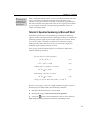
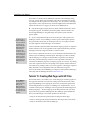
Tutorial 5: Using MathType’s Toolbar
In the previous tutorials we saw two formulas that were very similar, in the
sense that they had many terms in common. This is typical of many branches of
mathematics. For example, consider these formulas from elementary statistics:
σ2 =
1
k
{∑ X
σ XY
r =
=
σ XσY
2
i
}
− kµ2 =
1
1
2
∑ X i −
k
k
( ∑ X ) 
2
i
∑ X Y − k ( ∑ X )( ∑ Y )
1
i i
1

2
∑ X i −
k

i
i
( ∑ X )  ∑ Y
2
i
i
2
−
1
k
( ∑ Y ) 
2
i
Many statistical formulae use the symbols µ and σ, and they often involve
various combinations of terms like ∑ X i , ∑ X i2 , 1k . When dealing with repetitive
formulae like these you can save yourself a great deal of time by customizing
MathType. To save time creating statistical formulae, we’re going to place σ in
the Small Bar. We’ll also make expressions for ∑ X i and 1k , and place them in the
tabbed bars. Then we’ll use them to create the second of the equations shown
above. The steps are as follows:
32
Chapter 4: Tutorials
Toolbar Icon Sizes
Using the Workspace
Preferences command
on the Preferences
menu you can alter the
size of the toolbar icons.
1. Before we start, make sure that MathType’s toolbar is visible and that the
Small Bar and the Small and Large Tabbed Bars are visible. Use the commands in
the View menu to make them visible if necessary.
2. Click on the
palette will appear.
symbol palette, and then release the mouse button. The
3. Now hold down the ALT key, press on the σ and, keeping the left mouse
button down, drag it over the Small Bar. You’ll see the mouse pointer change
shape as it passes over different areas of the toolbar. When the pointer looks like
, the dragged item cannot be dropped at this location and releasing the
this
mouse button will have no effect. When the pointer looks like this it is over a
valid target area and releasing the mouse button will insert the object at this
location. Release the mouse button over the Small Bar, as shown below.
Adding New Symbols
You can add any
symbol from any font on
your computer to the
toolbar. Enter it into the
equation area, select it,
and drag it to the
toolbar. Use the Insert
Symbol dialog (on the
Edit menu — see
Tutorial 13 for details) to
locate the symbol, hold
down the ALT key and
drag the symbol to the
toolbar. As a result,
MathType has access to
a virtually limitless
supply of symbols.
The symbol will be added to the end of the bar. Now, to insert this symbol into
an equation you only need click on it in the Small Bar instead of hunting for it in
the palettes. The Small Bar is a good location for frequently used symbols as it is
always available and can contain many items.
4. Next, we’re going to add a ∑ X i expression to the Large Tabbed Bar. The
tabbed bars are similar to the Small Bar in how they operate, however they’re
divided into categories, which allows for a much larger number of items. Click
on the Statistics tab to display MathType’s default items for statistical equations.
There should be room for one more item in the Large Tabbed Bar (the bar has
room for 8 items). If there isn’t, select another tab that does have room.
5. Delete the current contents of the MathType window, and create the
template (not the
expression ∑ X i in the usual way. You’ll need to use the
template) to do this.
33
MathType User Manual
Editing Toolbar
Expressions
You can edit a toolbar
expression by doubleclicking. A new
MathType window will
open containing the
expression. Make your
changes, close the
window and the toolbar
will be updated.
7. To add this expression to the toolbar, select it and drag it to the Large
Tabbed Bar. When you release the mouse you’ll see the expression appear in the
bar.
8. Create an expression for
, in exactly the same way. Place this expression in
the Small Tabbed Bar. You can make the fraction full size, using the
template,
template. When you’re done, we’re
or you can make a case fraction using the
ready to create the formula
r=
σ XY
=
σ XσY

1
k
∑ X Y − 1k ( ∑ X )( ∑ Y )
1
2
∑ X i − k

i i
i
i
( ∑ X )  ∑ Y
2
i
i
2
−1
k
( ∑ Y ) 
2
i
9. Creating this formula doesn’t require any new techniques that you don’t
already know, so we’re not going to give you the usual step-by-step instructions.
Here are a few useful hints and reminders:
• You can insert σ by clicking on it in the Small Bar, which is much faster than
using the
palette.
• You can insert the term ∑ X i by clicking on it in the Large Tabbed Bar.
• A fast way to create ∑ Yi is to insert ∑ X i , drag across the X to select it, and
type Y to replace it.
• You can create ∑ X i2 by inserting ∑ X i and replacing the subscript template
with a sub/superscript template. To do this, select the subscript slot as shown
template. The CTRL
below, and hold down the CTRL key as you insert the
key causes the new template to replace the selected one instead of wrapping
around it. Then type 2 in the superscript slot.
• Note that the two terms inside curly brackets on the bottom line of the formula
are identical except that one involves X and the other involves Y. To create
the second term, just duplicate the first one and replace the X’s with Y’s.
• You can duplicate a term by selecting it, holding down the CTRL key and
dragging it to the desired location (without the CTRL key the term is moved).
Rearranging the Toolbar
MathType’s toolbar is initially filled with expressions useful for many of the
various fields in mathematics. You can, however, create your own tabs, rename
or delete the existing tabs, as well as rearrange or remove any of the symbols or
expressions that are in the default toolbar. You can also modify any of the
expressions if they’re not quite right for your particular use.
34
Chapter 4: Tutorials
To move a symbol or expression within the toolbar, hold down the ALT key and
drag the item to its new location. You can insert an item between two others by
dropping it between them.
10. Try this by dragging the σ symbol we added to the Small Bar in Step 3 to the
Small Tabbed Bar. The choice of where to place an item is entirely up to you; a
symbol or expression can be placed in any of the bars.
Now let’s delete the σ from the Small Tabbed Bar.
Deleting Toolbar Items
Another way to delete
an item is to ALT-drag it
from the bar and release
the mouse over an
invalid target, e.g.
outside the MathType
window.
11. Right-click on the σ and select Delete from the context menu that appears.
You may also want to delete the other expressions you added to the tabbed bars.
You can also change the names of the tabs to suit your particular situation.
12. Double-click on the Statistics tab to open the Tab Properties dialog, where
you can edit the tab’s name and change its keyboard shortcut.
If you prefer typing to using the mouse, you may want to use the toolbar’s
keyboard interface. You can give the keyboard focus to a toolbar component
using the following keyboard commands:
Symbol Palette
F5
Template Palette
F6
Small Bar
F7
Large Tabbed Bar
F8
Small Tabbed Bar
F9
Once a bar has the focus, you can use the left and right arrows to move the
selection, and ENTER to insert the selected item (or open its corresponding menu).
The ESC key closes a menu, or returns the focus to the equation area. You can
switch tabs by typing CTRL+F10, n where n is the number of the tab to activate.
For example, typing CTRL+F10, 2 activates the second tab.
Deciding What to Place in the Toolbar
Keyboard Shortcuts
Keyboard shortcuts are
covered in more detail in
Tutorial 16.
Some symbols and templates are used so frequently that you may not need to
place them in the toolbar. You probably will have memorized the keyboard
shortcuts for inserting them, so there’s not much to be gained by having them
occupy valuable space in the toolbar. Greek symbols in particular fall into this
category; once you’ve learned that you can insert a β by pressing CTRL+G
followed by b (referred to as CTRL+G,B), you probably won’t need to add these
characters to the toolbar.
Insert Symbol Dialog
Using this dialog is
covered in more detail in
Tutorial 13.
It may make sense, however, to add characters from any special fonts you may
have to the toolbar. The easiest method is to use the Insert Symbol dialog (choose
the Insert Symbol command on the Edit menu), which is an extremely powerful
tool for viewing the characters in a font. You can also ALT-drag characters from
35
MathType User Manual
this dialog to the toolbar. You can add as many characters from your fonts to the
toolbar as can fit. Then you can enter these characters at any time into your
equations, regardless of your current style definitions.
That does it for Tutorial 5, so choose Select All (CTRL+A) from the Edit menu and
press BACKSPACE or DELETE to clear the window for the next tutorial.
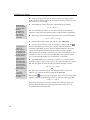
Tutorial 6: Spacing and Alignment
In our next example we introduce some of MathType’s facilities for controlling
spacing and alignment in equations. We are going to create the following pair of
equations:
∫
∫
1
0
1
0
a ( x) dx ≤ limsup φ n (a)
n→∞
a( x)b( x) dx ≤ limsup ψ n (a, b)
n→∞
Note that these equations are arranged so that their ≤ signs are vertically aligned,
and they both contain a “lim sup” construction of a type that we have not used
before. You can create these equations as follows:
36
Expanding Integrals
Integral signs are
normally a constant
size. You can create an
expanding integral by
holding down the SHIFT
key while you choose an
integral template from
the integrals palette.
1. Insert a definite integral template by clicking on the icon or by pressing
CTRL+I, type in the integrand (the large slot), and fill in the 0 and 1 as the limits
of integration (the two small slots). You probably won’t want the parentheses in
the integrand to be of the “expanding” variety, so you can just type them from
template. Your equation should now look
the keyboard, rather than using the
like this:
Parentheses Template
You may prefer to use
the template instead of
typing ( and ). Using the
template can give your
document a more
consistent look. The
template also includes
more space around it,
so you may not need to
add the thin space as
shown here. We’re
trying to teach you the
different ways to create
equations; obviously the
final choice is up to you!
2. To improve the appearance of our equation, we should insert a thin space
(one sixth of an em) in between the a(x) and the dx in the integrand. MathType
can not do this automatically, so we provide you with a convenient way of
palette provides a set of
manually entering a space of the correct size. The
five icons representing commonly used spaces, as shown in the following table.
Icon
Keystroke
SHIFT+SPACE
CTRL+ALT+SPACE
CTRL+SPACE
CTRL+SHIFT+SPACE
None
Alt. Keystroke
CTRL+K,0
CTRL+K,1
CTRL+K,2
CTRL+K,3
CTRL+K,4
Description
Zero space
One point space
Thin space (sixth of an em)
Thick space (third of an em)
Em space (quad)
Place the insertion point between the “)” and the “d” by clicking there, and insert
icon (it’s on the right in the top row of the
a thin space either by choosing the
palette) or by pressing CTRL+SPACEBAR.
Chapter 4: Tutorials
Show Nesting
The Show Nesting
command on the View
menu shows the
different slots and can
help you avoid making
mistakes.
3. Move the insertion point out of the integrand slot, into the position shown
below. You must do this for the alignment commands to work properly. Don’t
create the rest of the equation within the integrand slot.
4. Click on the ≤ sign in the Small Bar.
5. Now we want to build the “lim sup” structure. We begin by clicking on the
icon in the
Palette. This icon represents an underscript template: any
characters entered in the upper slot will be full size, and those in the lower slot
will be reduced to “subscript” size.
6. The insertion point is positioned in the upper slot, so you can type in
limsup. MathType will use your “Function” style (probably a plain style) for
these characters, and will insert a thin space between the “lim” and the “sup”.
7. Move the insertion point down into the lower slot by clicking in it or by
pressing the TAB key, and enter n→∞. The → and ∞ symbols are very common
in mathematics, so they’ve been added to MathType’s default Small Bar. They’re
also available in the Symbol Palettes, of course. Following typesetting
conventions (as always), MathType will not create any spacing around the →
symbol, since it is in a “subscript,” but you can insert spaces, if you want to.
One-Shot Shortcuts
The shortcuts that affect
just the next character
typed are described in
more detail in Chapter 7.
8. Press TAB to move the insertion point out of the lower slot, and type in the
rest of this first equation. The speedy way to do this is to just type CTRL+G f
CTRL+L n TAB ( a ). If you like the CTRL+G shortcut, you may be interested to
know that there are a few others that work in a similar fashion. If you press
CTRL+U, for example, the next character you type will be assigned the User 1
style that you have defined with the Define command on the Style menu. In this
way, you can access any character in any font with just two keystrokes, even if
it’s not present in the Symbol Palettes.
9. Press the ENTER key. This will create a new line directly beneath the first
equation, so now you have a “pile” consisting of two lines. It should look like
this:
37
MathType User Manual
Selecting a Slot
You can double-click in
a slot to select its
contents, or type
CTRL+SHIFT+S.
10. To save time, we’re going to create the second equation by modifying a copy
of the first one. Select the entire first equation by double-clicking somewhere
near its ≤ sign, copy it to the clipboard, and then paste it into the new empty slot.
You should now have two identical copies of the first equation, one directly
beneath the other. Now just edit the lower copy to produce the second equation.
To change the φ to a ψ, just select the φ and press CTRL+G followed by y.
11. Finally, we’re going to experiment with some different ways of aligning the
two equations. You can center or right-justify them by using the Align Center
and Align Right commands on the Format menu. Give this a try, just to see how
it looks.
12. In fact, you will probably want to align these two equations so that their ≤
signs are directly above one another. To do this, we choose the Align at =
command from the Format menu. It will work even though we have ≤ signs
rather than = signs. You can align the equations in other ways by using
alignment symbols. You simply insert an alignment symbol in each equation at
the two points that you’d like to have aligned. (However, note that alignment
symbols inserted into template slots will not work.) Placing an alignment symbol
to the right of each of the two ≤ signs would give the same results as using the
Align at = command, for instance. The alignment symbol is represented by the
icon in the Symbol Palettes — it’s located in the
palette.
13. You may also want to adjust the line spacing, or leading, i.e. the amount of
vertical space between the two equations. You can do this by placing the
insertion point somewhere in the outermost slot of the second equation (not
within a template), or by selecting the second equation, and choosing the Line
Spacing command from the Format menu. When you’ve arranged them to your
liking, the equations are complete.
Now that we’re done with these equations, it’s time to choose Select All from the
Edit menu and press BACKSPACE to clear your window for the next tutorial.
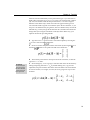
Tutorial 7: A Simple Matrix
In our next tutorial, we illustrate MathType’s powerful capabilities for laying out
matrices. We will construct the following matrix equation:
p(λ ) = det( λ I − A ) =
λ − a11
− a12
− a21
λ − a22
The matrix is a fairly simple one, and we’ll be able to create it very easily by
using a matrix template. If you need more flexible formatting capabilities for
matrices and tabular layouts, you should use tabs, as illustrated in Tutorial 11.
1. Type the first few terms of the equation, up to the second equals sign.
MathType will recognize that “det” is an abbreviation for the determinant
38
Chapter 4: Tutorials
function, and will automatically set it in plain roman type, so you don’t have to
fiddle with it. The quick way to get a λ is to press CTRL+G followed by a letter l
(ell). Also, note that the I and the A represent matrices, so we have assigned
them the Vector-Matrix style, which causes them to appear in bold type. The
CTRL+B shortcut will assign the Vector-Matrix style to the next character, so you
can press CTRL+B followed by I to get the I, and CTRL+B followed by A for the A.
Alternatively, you can just type all the characters first, and then select them and
change their styles using the commands on the Style menu. Either way, your
equation should end up looking like this:
2. Type the second = sign and insert a vertical bar template by choosing the
icon. It’s located in the
palette.
3. Insert a 2×2 matrix template inside the vertical bars by choosing the
from the
icon
palette. Your equation should now look like this:
4. The insertion point will be in the top left slot of the 2×2 matrix, so enter the
expression λ – a11 there.
Drag and Drop
You can also drag the
term and drop it in the
other slots. Remember
to hold down the CTRL
key to copy the term.
5. We’re feeling lazy, so we’re going to create the other entries in the matrix by
cutting and pasting. Select the λ – a11 by double-clicking on it, copy it to the
Clipboard, and paste it into the other three slots in the matrix. The result should
be as shown below; it’s not right, of course, but we’re going to fix it up in a few
moments.
39
MathType User Manual
6. Next, we’re going to put a little extra space between the vertical bars and the
elements of the matrix. This is purely a matter of taste, so you can skip this part if
you’d prefer to keep your matrix looking the way it does at present. Before we
enter the spaces, we need to position the insertion point so that it’s inside the
vertical bars but to the left of and outside the matrix. You can do this by clicking
somewhere near the position indicated by the arrow pointer in the preceding
picture. Then just enter one or two thin spaces by pressing CTRL+SPACEBAR. Do
the same on the right-hand side of the matrix. If you choose the Show All
command from the View menu, you’ll be able to see your spaces. They should
look like this:
7. After the brief digression in Step 6, it’s now time to correct the entries in our
matrix. First, delete the λ from the upper right slot. The quickest way to do this is
to place the insertion point to the right of it and press BACKSPACE (or Backspace).
Do the same with the λ in the lower left slot. Notice that MathType adjusts the
spacing after the minus signs to reflect the fact that they are now unary operators
rather than binary operators (negation rather than subtraction).
8. Change all the subscripts in the matrix to their desired values. The “11” in
the upper left slot is correct already, but we should have “12” in the upper right
slot, “21” in the lower left, and “22” in the lower right. You can double-click on
the existing subscripts to select them, and then type the correct values over them,
just as you would in a word processor. Your equation should now look like this:
Modifying a Matrix
The Matrix submenu on
the Format menu
contains commands for
adding and deleting
rows and columns.
9. The equation is now essentially complete, although there are a few more
formatting options that you may want to try out. First, you might want to shift
the entire matrix down so that its top row is aligned with the rest of the equation.
To do this, place the insertion point anywhere in the matrix and choose Align at
Top from the Format menu. Also, it might be nice to right justify the entries in
each column. To do this, place the insertion point somewhere in the matrix,
choose the Change Matrix command from the Matrix submenu on the Format
menu, and click on the button labeled “Right” in the dialog box.
Finally, if you object to the fact that MathType tightened the spacing after the
unary minus signs, you can put the spaces back in again, though this would
mean deviating from standard typesetting conventions. They should be thick
spaces (one third of an em). The thick space is the middle one in the second row
40
Chapter 4: Tutorials
palette. If you prefer to use the keyboard, you can insert a thick
of the
space by pressing CTRL+SHIFT+SPACE. Alternatively, since a thick space is the
same width as two thin spaces, you can get the same results by pressing
CTRL+SPACE twice.
If you elected to make all of the modifications suggested in this step, your
equation should look something like the picture below.
If you’re going on to the next tutorial, press CTRL+A to select all, then press
BACKSPACE or DELETE to clear your screen.
Tutorial 8: Fonts and Styles
This tutorial provides an introduction to MathType’s system of styles. We will
demonstrate how to change the fonts in your equations by changing style
definitions. Using styles will allow you to achieve the formatting you want
quickly and easily, and enable you to create equations with a consistent
appearance. See Chapter 7 for more information about styles, fonts and sizes.
In the following steps, we will create the equation
u = φ ⋅ exp { 12 σ ( x + y )}
and experiment with changing the look of the equation by using different style
definitions.
1. Check that the Status Bar’s Style panel displays “Math”. If it doesn’t, choose
Math from the Style menu. If the Math style is not chosen, MathType’s automatic
style assignment will not be in effect, and the rest of this tutorial will not make
much sense.
template for the fraction and inserting the
φ and σ by choosing them from the lowercase Greek palette, or by using the
palette. The equation
CTRL+G shortcut. The “ ⋅ ” operator is located on the
should now look like this:
2. Create the equation, using the
41
MathType User Manual
Define Styles
You can also open this
dialog by double-clicking
in the Style panel of the
Status Bar.
3. From the Style menu, choose Define. If necessary, click on the Simple button
to display the dialog shown below.
The TEX Look
Change the “Primary font” to Euclid, change the “Greek and math fonts” to
Euclid Symbol and Euclid Extra, as shown in the dialog above, and then click
Apply. On screen, your equation will now look like this:
We’ve included a
MathType preference
file called TeXLook.eqp
that contains font and
spacing settings that
make MathType
equations look like TEX.
It’s in the Preferences
folder inside your
MathType folder. See
Chapter 7 for more
details on using
preference files.
and if printed will look like this:
u = φ ⋅ exp { 12 σ(x + y )}
The Euclid fonts supplied with MathType are based on the Computer Modern
fonts typically used with TEX, so they give your documents a TEX-like
appearance that you might prefer for some types of work. Another benefit of the
Euclid fonts is that their regular and Greek characters have a consistent size,
whereas Times and Symbol are somewhat mismatched. Of course, if you use the
Euclid fonts in your equations, you will probably want to use Euclid as the
primary body font in your word processing document, too.
3. Open the Define Styles dialog, and click on “Factory settings” to return to
using the Times and Symbol fonts.
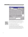
4. Click on the Advanced button to display a more extensive form of the
Define Styles dialog. This is shown below:
42
Chapter 4: Tutorials
TIP
The changes you make
in this dialog apply to
the current equation.
Check “Use for new
equations” to use the
settings for new
equations as well.
The names of the eleven styles are listed in the dialog box, together with the font
and character style assigned to each. The equation you have just created uses the
Function, Variable, L.C. Greek, Number, and Symbol styles. The letters “exp” are
recognized as the abbreviation for the exponential function, and are assigned the
Function style; u, x, and y are treated as variables and assigned the Variable
style; φ and σ, being lowercase Greek letters, are assigned the L.C. (lowercase)
Greek style, and the numbers in the fraction use the Number style. The symbols
=, ⋅, (, ), and + use the Symbol style. (The angle brackets and fraction bar are
internal to MathType and do not use a style.) These styles are applied
automatically as you create the equation, because you are using the Math style
mode. This automatic style assignment is the advantage you gain by using the
Math style mode when creating equations.
More About Styles
The subject of
MathType’s styles is
covered in more detail in
Chapter 7.
We’re going to change some of the styles so you understand how they affect an
equation’s appearance. Normally you wouldn’t work this way, you’d change
fonts using the Simple version of this dialog.
5. Choose a new font for the Function style. The style is probably defined as
Times or Times New Roman. Press on the arrow next to the font name in the
Function row and choose a different font. You will want to choose a font that
looks noticeably different from Times, so that the effect of the change will be
obvious. A good choice would be a sans serif font such as Arial.
43
MathType User Manual
6. Choose the OK button. Your equation will be redisplayed using the new
Function style definition. Your equation should now look like this:
The function abbreviation, exp, is displayed using the new font. Of course, you
probably wouldn’t want your equation to look like this — we’re simply
demonstrating the effect of changing the Function style definition.
The Variable style definition is used for all ordinary alphabetic characters except
for the ones in function abbreviations. In the current equation, this includes u, x,
and y. Very often, according to convention, the only difference you want
between the Variable and Function styles is for the Variable style to be defined as
italic. Let’s redefine the Variable style so that it’s consistent with the new
Function style definition.
Choosing Fonts
A fast way to select a
font is to click in the list
and then type the first
letter of the name. You
can also use the scroll
bar in the list to move
around quickly.
7. Again, choose Define from the Style menu. In the Define Styles dialog box,
press on the arrow next to font name in the Variable row, and choose the same
font assigned to the Function style. Check that the italic character style is checked
for Variable, but not for Function.
Let’s also change the Number style so that it uses the same font as Function and
Variable. You will find that this makes the equation look better. Finally, turn off
the italic character style for the L.C. Greek style by removing the check in the
Character Style column. Lowercase Greek letters are usually italicized, but let’s
experiment with this. Note that for the two Greek styles and the Symbol style
you can only assign fonts with the same encoding (arrangement of characters) as
the Symbol font. This typically restricts your choice to the Symbol font, the
Euclid Symbol font, or some other similar font.
8. Choose the OK button. Your equation will be redisplayed using the new
style definitions. If you are using the fonts we’ve recommended, the equation
should now look like this:
The “variables” u, x, and y, and the numbers in the fraction 12 now use the new
font definitions, and the lower-case Greek letters φ and σ are no longer italicized.
You may want to use style definitions such as these for equations in a document
in which the text is written in Arial or Tahoma. When printed, the equation will
look like this:
u = φ ⋅ exp { 21 σ( x + y )}
To reset the style definitions, open the Define Styles dialog and click “Factory
settings”.
44
Chapter 4: Tutorials
TIP
You can also right-click
in the Style panel of the
Status Bar to make the
Style menu appear.
While working through this tutorial, you have probably noticed that each of the
styles is also listed as a command on the Style menu. This allows you to
explicitly assign a particular style to selected or subsequently-typed characters.
The Other command on the Style menu can be used to assign any font available
on your computer to selected or subsequently-typed characters. Please see
Chapter 7 for further details.
Tutorial 9: Equation Numbering in Microsoft Word
This tutorial describes how to use the MathType commands for numbering
equations in Microsoft Word documents. Although Word has its own method for
numbering equations (captions), Word places captions above or below an item,
not to the side, which is typically how equations are numbered. Using the
MathType toolbar that’s added to Word, you can enter inline, display and
numbered display equations with just one click.
We’re going to create the following portion of a document to illustrate the
equation numbering commands.
We now have two basic equations:
cos 2 θ + sin2 θ = 1
(1.1)
cos 2 θ − sin2 θ = cos 2θ
(1.2)
Adding these two together, we obtain
cos 2 θ = 12 (1 + cos 2θ)
(1.3)
Subtracting (1.2) from (1.1) gives
sin2 θ = 12 (1 − cos 2θ)
(1.4)
Using (1.4) we can show that cos 2θ = 1 − 2 sin2 θ.
However, we’re going to create it in a slightly unrealistic sequence, in order to
illustrate the power and flexibility of the numbering commands.
1. Run Microsoft Word and create a new document.
2. Enter the following text: We now have two basic equations:
3. Click on the
button on Word’s MathType toolbar, or choose the Insert
Right-Numbered Display Equation command on the MathType menu.
45
MathType User Manual
4. A dialog will appear asking if you want to create a new chapter/section
break at the start of this document. We’ll explain the meaning of this later in the
tutorial. For now, just click OK.
Word Styles Used
The line containing the
equation is formatted
with Word’s
MTDisplayEquation
style, which you can
modify to affect all
display equations in
your document.
5. In the MathType window that opens, enter the following equation:
cos 2 θ + sin2 θ = 1
then close the MathType window. In your Word document, notice that the
equation is centered and the equation number is aligned with the right margin.
6. Repeat step 3 and insert the following equation into your Word document:
cos 2 θ − sin2 θ = cos 2θ
7. Enter the following text at the start of the next line: Subtracting
Equation References
8. Now let’s insert a reference to the second display equation. Click the
• You can jump to an
equation in your
document quickly by
double-clicking on any
of its references. Then
press SHIFT+F5 to jump
back to the reference.
button on the MathType toolbar or choose the Insert Equation Reference
command on the MathType menu. The Insert Equation Reference dialog will
appear, displaying brief instructions about inserting an equation number
reference. Once you are familiar with the process you can click the “Don’t show
me again” box. For now, click OK, then double-click on the equation number
(1.2). You’ll see that the number (1.2) is inserted into your sentence.
• In large documents try
splitting your window
into two panes (search
for split in Word’s Help).
Insert the references in
one pane and scroll and
double-click on the
equation numbers in the
other.
• You can place
equation number
references in footnotes
and endnotes.
9. Type from and then enter a reference to equation (1.1) using the method
described in step 8. You may want to enter a space before and after the reference.
10. Then type gives and insert the following numbered display equation:
sin2 θ = 12 (1 − cos 2θ)
11. At the start of the following line, type Using and insert a reference to
equation (1.3). Complete the line by typing we can show that
12. Click the
button on Word’s MathType toolbar, or choose the Insert Inline
Equation command on the MathType menu, and insert the following equation:
cos 2θ = 1 − 2 sin2 θ.
Notice how this equation is inserted in the line of text (hence the name inline
equation). Word also aligns the equation with the baseline of the text. Your
document should now look like this:
46
Chapter 4: Tutorials
We now have two basic equations:
cos 2 θ + sin2 θ = 1
(1.1)
cos 2 θ − sin2 θ = cos 2θ
(1.2)
Subtracting (1.2) from (1.1) gives
sin2 θ = 12 (1 − cos 2θ)
(1.3)
Using (1.3) we can show that cos 2θ = 1 − 2 sin2 θ.
Now we’ll insert another equation in the middle of this example to demonstrate
automatic renumbering.
13. Place the insertion point before the word Subtracting, and enter the
following text: Adding these two together, we obtain
Equation Numbers
You can insert just an
equation number using
the Insert Equation
Number command.
If Updating Is Slow
If updating takes too
long, uncheck “Update
equation numbers
automatically” in the
Format Equation
Numbers dialog. Then
use the Update
Equation Numbers
command to manually
update the numbers.
14. Insert this numbered display equation:
cos 2 θ = 12 (1 + cos 2θ)
You’ll see that the new equation is numbered (1.3), and the following equation
number and its reference have been renumbered to (1.4). Your document should
now look like the example at the start of this tutorial.
Whenever you insert an equation number or an equation reference, all numbers
in the document are updated. However, if you move or delete an equation
number, you must use the Update Equation Numbers command on the
MathType menu to regenerate the number sequence. Also, be aware that
deleting an equation number does not automatically delete any of its references;
you’ll have to do this yourself. You can find them by using the Update Equation
Numbers command, which will cause Word to display an error message in place
of each reference. You can then delete them.
Equation Number Formats
You can also control the format of the equation numbers.
Whole Document
To change the format of
existing equation
numbers you must
check the Whole
Document checkbox.
Otherwise you’re only
setting the format for the
next number(s) you
insert.
15. Choose the Format Equation Numbers command on the MathType menu
(there’s no toolbar button for this command). Check the Whole Document
checkbox (to change the existing numbers) and change the Enclosure option to
<> (angle brackets). The preview shows you the result of your settings. Click OK,
and you’ll see the equation numbers and references change to the new format.
You may want to experiment with some of the settings — there are many
possible combinations.
47
MathType User Manual
Chapter/Section Breaks
Section Numbers
If you don’t want section
numbers included, you
can turn them off in the
Format Equation
Numbers dialog.
The default equation number format includes a section number and an equation
number, e.g. (1.1). You can also include a chapter number if needed. The chapter
and section numbers are determined by the nearest preceding Chapter/Section
Break in your document. You insert and modify these breaks using commands
on the MathType menu. We already inserted one at the start of this document as
part of inserting the first equation number. Now we’ll change its value.
Show Chapter/Section
Breaks
You can show and hide
chapter/section breaks
by clicking on the
button in Word’s toolbar.
This shows and hides
the MTEquationSection
style.
16. Choose the Modify Chapter/Section Break command on the MathType
menu. The location of the section break will be highlighted and the Modify
Chapter/Section Break dialog will open. Let’s assume we’re working on
Section 2 of a book, so we want the section number to be 2 and the equation
number to be 1. Choose the “Section number:” button and enter 2. The “Next”
option can be useful if your document contains several sections and you want
them numbered sequentially. (Remember that there’s no link between Word’s
sections and MathType’s chapter/section breaks; it’s up to you to associate them
by placing the breaks in the appropriate places in your document). Now click
OK. The chapter/section break will be hidden, and the equation numbers in the
document will all start with 2.
If you’ve followed these steps your document should look something like this:
We now have two basic equations:
cos 2 θ + sin2 θ = 1
<2.1>
cos 2 θ − sin2 θ = cos 2θ
<2.2>
Adding these two together, we obtain
cos 2 θ = 12 (1 + cos 2θ)
<2.3>
Subtracting <2.2> from <2.1> gives
sin2 θ = 12 (1 − cos 2θ)
<2.4>
Using <2.4> we can show that cos 2θ = 1 − 2 sin2 θ.
MathType’s equation numbering commands can also support three levels of
numbering, e.g. chapter, section and equation numbers. You can also control the
format of the numbers and create your own custom formats. The following
tutorial shows you how to do this; we’ll use the document we created in this
tutorial so don’t delete it!
48
Chapter 4: Tutorials
Tutorial 10: Advanced Equation Numbering in
Microsoft Word
The simple equation numbering example shown in the previous tutorial is
sufficient for many documents, but sometimes you may need to create a third
level of numbers. For example your document may require chapter, section and
equation numbers. Or, you may find that the built-in number formats don’t
match your needs and you’d like to create a custom number format. This tutorial
shows you how to accomplish both tasks.
1. Open the document you created in the previous tutorial.
2. Open the Format Equation Numbers dialog by choosing the Format
Equation Numbers command on the MathType menu.
49
MathType User Manual
3. The settings should appear as shown above. The top group of items controls
the number format. We want to add a chapter number, so check the “Chapter
Number” checkbox. Notice how the preview changes to <1.1.1>).
4. Check the “Whole document” checkbox so that the changes we make will be
applied to existing equation numbers. Then click OK.
You’ll notice that the document has changed, and the equation numbers now
read <1.2.1>, <1.2.2> etc. This is because the chapter/section break at the start of
the document sets the chapter number to 1. This was added to the document
when we inserted the first equation number. Let’s pretend we want to set this to
be Chapter 2.
5. Choose the Modify Chapter/Section Break command on the MathType
menu, and the following dialog will open. You’ll see that the break itself has also
been made visible in the Word document.
6. Change the Chapter number value to 2 and click OK. The numbers in the
document should now read <2.2.1>, <2.2.2> etc.
Now let’s try changing the format of the numbers more dramatically. We’ll set
the format so that the numbers read Equation 2.2.1, Equation 2.2.2 etc.
7. Choose the Format Equation Numbers command on the MathType menu.
Select the Advanced Format radio button, and enter Equation #C1.#S1.#E1 in
the edit box. You’ll see how the Preview changes.
8. Check the “Whole document” checkbox, and click OK. The equation
numbers in the document should be updated.
You can experiment with different custom formats in this manner. The
‘language’ used for the formats is very simple, all characters are used literally
except for the constructs #Cx, #Sx and #Ex, where x indicates the numeric
representation and can be one of 1,a,A,i,I.
50
Chapter 4: Tutorials
A fast way of learning how to control the formatting is to select the Simple
Format button, and then change the various options. The Advanced Format text
is still visible, and it updates every time you make a change to the built-in
formats. Full details are in the Help for this dialog.
Tutorial 11: Setting Up a Microsoft Word Document
When creating a Microsoft Word document containing equations there are
several considerations you should keep in mind. You’ll probably want the body
text to match the equations in terms of fonts and sizes, and you’ll typically want
all equations in the document to use consistent formatting, i.e. the same font and
size settings, as well as any other special settings you may have made in
MathType.
This tutorial shows you how to achieve these goals, and how to update the
document’s equations if you decide to change your fonts and/or sizes.
Word’s Styles
If you’re not familiar with
Word’s styles we urge
you to take a few
minutes to learn how to
use them. In Word’s
Help Contents, search
for styles.
Although Word and MathType allow you to select text and change its font and
size directly, we strongly recommend that you make use of styles, instead. Both
programs use this approach because it makes modifying the look of a document
or equation very easy. You simply change the definition of a style (e.g. from
Times New Roman to Arial, or from 12 pt plain to 10 pt italic), and your
document or equation is immediately reformatted with the new settings.
Let’s assume that you’re required to produce a document where the body font is
10 pt Times New Roman. The first step is to define MathType’s settings to match
the Word document.
1. In MathType, open the Define Styles dialog and set the main font to Times
New Roman using either the Simple or Advanced pane. Make sure the “Use for
new equations” box is checked, and click OK.
Factory Settings
Click “Factory settings”
to reset the values.
Equation Preferences
The definitions of all the
styles, sizes, and
spacing used in an
equation are referred to
collectively as “equation
preferences”. See
Chapter 7 for more
details.
2. Open the Define Sizes dialog and set the Full size to 10 pt. As the other
dimensions are by default expressed as percentages, MathType will calculate
them for you. Again, check the “Use for new equations” option, and click OK.
3. Back in Word, choose the Set Equation Preferences command on the
MathType menu. Make sure the “MathType’s ‘New Equation’ preferences”
option is selected. This means that whenever you create a new equation using
the commands on the MathType menu or MathType toolbar, the settings
MathType is currently set to use for new equations are the ones that will be used.
Click OK to close this dialog.
Note: you may not always want to rely on MathType’s ‘New Equation’
preferences. If you tend to change MathType’s size and style definitions quite
often, you may want to create a MathType preference file, and then choose this
file in the Set Equation Preferences dialog. This will copy the file’s preferences
into your Word document, so that no matter what changes you make to
51
MathType User Manual
MathType, equations created in your document will always use these
preferences.
4. Now we’ll quickly create a Word style for the body of the document. Choose
the Style command on Word’s Format menu, click New and name the new style
“body”. You’ll probably base it on Word’s built-in normal style. Set the new
style’s font to Times New Roman 10 pt by clicking on the Format button and
choosing Font. Click OK to close the Font dialog.
Line Spacing
For a more detailed
discussion of this issue
see the Using MathType
with Microsoft Word
section of Chapter 5.
5. Click on the Format button again and this time choose Paragraph. In the
dialog’s Indents and Spacing page, change the Line Spacing option to Exactly,
and type 12 pt in the accompanying text box. This forces Word to use this value
when spacing lines of text, and prevents Word applying extra spacing around
lines that contain inline equations. Click OK to close the dialog.
6. Click OK to close the New Style dialog, and then click Apply to close the
Style dialog.
You’ve now configured Word and MathType to use the same font and size
definitions, which will make equations closely match the look of the rest of the
document. Go ahead and enter a line or two of text and insert a simple equation.
Now let’s suppose that, as so frequently happens, you have to change the
document’s font to Garamond. To keep this example simple we won’t change the
point size, but you’d follow the same steps if this were the case.
These are the changes we need to make:
• Modify Word’s “body” style to use Garamond instead of Times New Roman.
• Modify MathType’s styles to use Garamond instead of Times New Roman.
• Update the existing equations in the document to use the new font.
The first two steps are very similar to how we originally created the styles and
added them to the Word document, so we won’t go through them in detail. The
first step involves using Word’s Style dialog, the second step requires
MathType’s Define Styles dialog.
The third step involves the Format Equations command on the MathType menu.
7. Choose the Format Equations command, and the Format Equations dialog
will appear. This dialog allows you to reformat the equations in your document,
and provides you with several ways to determine the equation preferences that
are applied. The choices are:
• The equation preferences already stored in this document.
• MathType’s current equation preferences for new equations.
• The equation preferences contained in a MathType equation you’ve copied to
the clipboard.
52
Chapter 4: Tutorials
• The equation preferences contained in a MathType preference file.
TIP
Click Help for more
details on the other
options.
For this example click the “MathType’s ‘New Equations’ preferences” button.
You can click Preview to get a list of the actual preferences.
8. Click OK and the formatting process will start. This can take anywhere from
a few seconds to several minutes depending on the speed of your computer and
the number of equations in your document. The command’s progress is shown
in Word’s status bar. When the operation has finished, check that the equations
were updated.
Tutorial 12: Formatting with Tabs
In this example we show you how MathType’s system of tabs provides extra
flexibility for formatting equations. We’re going to create the equation:
 1
 + 9.76 x
cn ( x) =  k

14.3 x
when n is even
when n is odd
and then format it several different ways. We proceed as follows:
1. Create the expression on the left-hand side of the equals sign. As you know
by now, you can choose the
to the c.
2. Choose the
template or press CTRL+L to attach the subscript
template from the
brace. You should now have the following:
palette to insert an expanding left
3. Enter the top expression in the brace, up to and including the x, and then
press CTRL+TAB (press the TAB key while holding down the CTRL key). If you
press the TAB key alone, this will move the insertion point, rather than insert a
tab character.
Choosing Styles
Another way to choose
a style is to right-click in
the Style panel of the
status bar and select the
style from the context
menu that appears.
4. Choose the Text style from the Style menu and type in when n is even.
While you’re using the Text style, the spacebar is active and you have to type
spaces, as you would in a word processor. Choose Show All from the View
menu, if it’s not already checked, so that you can see your tab character, which is
displayed as a small diamond. Also, choose Ruler from the View menu if it’s not
already checked. Your equation should look like this:
53
MathType User Manual
Note that the tab character causes the phrase “when n is even” to line up
underneath the first default tab stop to the right of the x. The default tab stops
(indicated by small inverted T’s along the Ruler scale) are positioned at half-inch
intervals starting at the left-hand side of the current slot. Since we are currently
template, the half-inch intervals are measured
within the main slot of the
from the left edge of this slot, i.e. just to the left of 1 .
k
5. Press ENTER to start a new line underneath the first one, and type in its
contents. You should switch back to the Math style to enter 14.3x, and switch
back to Text again to type when n is odd. Insert a tab character (CTRL+TAB) after
the x, as in the first line. This should give you:
Again, the text phrase aligns with the first default tab stop to the right of the x.
template, and that each
Note that you have created a two-line pile within the
pile in MathType has its own tab stops.
Changing Styles
Remember you can also
use the keyboard
shortcuts listed on the
Style menu, or right-click
on the Status Bar’s Style
panel.
6. Select the n in the first line and choose Math from the Style menu. This
makes MathType interpret the n as a mathematical quantity, i.e. a variable, and
will therefore apply the Variable style (typically italic). Do the same to the n in
the second line.
7. Place the insertion point somewhere within one of the two lines on the righttab well, and then click on the Ruler at
hand side of the equation, click on the
about the 1½ inch mark to set a left tab stop. This will remove all default tab
stops to the left of the new tab stop. Your equation should now be aligned as
shown below:
If this is how we want the equation formatted, then our work is finished.
However, there are several other options that are worth exploring.
8. First, we’re going to align the two x’s. Insert a tab character (CTRL+TAB) at
the start of each of the two lines. This will cause each line to be shifted so that its
left-hand side aligns with the left tab stop. The text phrase in each line, since it is
separated by another tab character, will align with the first available default tab
stop to the right of the x.
54
Chapter 4: Tutorials
9. Next, click on the tab well, and then click on the Ruler just to the left of
the previous tab stop. This should produce the following results:
You can now change the formatting easily by just dragging the tab stops around
on the Ruler.
10. Next, we’re going to align the two decimal points. To prepare for this, first
remove the tab by dragging it downwards away from the Ruler and then
tab well, and then click on the
releasing the mouse button. Next, click on the
Ruler at around the one inch mark to set a decimal tab stop. Your equation
should end up looking like this:
That’s it for this tutorial, so delete your equation to be ready for the next tutorial.
Tutorial 13: Inserting Unusual Symbols
In this tutorial, you'll learn how to use MathType's Insert Symbol dialog to locate
and use symbols that are not readily available in the built-in palettes. Suppose,
for example, that you are going to be writing a document about some newlyinvented operations on sets that are analogous to conventional union and
intersection. You will want to find symbols to represent your new set operations,
and it would be nice if these were similar to the conventional ∪ and ∩ symbols.
Your first attempt might be to use bold versions of the conventional symbols to
represent your new operations, like this:
A∪ B = A∪ B
A∩ B = A∩ B
Unfortunately, the bold symbols look too much like the regular ones, so we'll try
to find a better solution.
1. Create the equations as shown above.
55
MathType User Manual
2. From MathType’s Edit menu, choose Insert Symbol. The following dialog
will appear:
This dialog is somewhat similar to the one in Microsoft Word, and to the
Windows Character Map accessory, which you may already know how to use.
Getting Detailed Help
To get detailed
information about the
Insert Symbol dialog,
click on the Help button
near its upper right-hand
corner.
You can use the Insert Symbol dialog to browse all the fonts available on your
computer, and investigate MathType’s knowledge of them. Specifically, you can:
• Insert a specific character or mathematical symbol into your equation.
• Add a frequently used symbol to the toolbar.
• Add a keyboard shortcut for a frequently used symbol.
• Find a symbol by matching words in its description.
3. The first place to look for usable symbols is the Symbol font, so select
Symbol from the list of fonts near the top of the Insert Symbol dialog. A quick
way to locate a font is to click on the list and then type the first letter or two of
the font’s name. Once the desired font is selected you can scroll through the large
grid of characters in the center of the dialog, looking for likely prospects.
56
Chapter 4: Tutorials
Larger Symbol Display
To enlarge the
characters in the Insert
Symbol dialog, choose
Workspace Preferences
from MathType's
Preferences menu, and
set Toolbar size to
Medium or Large.
4. You might also look in the Euclid Symbol and Wingdings fonts. Note that
the Insert Symbol dialog tells you that Symbol and Euclid Symbol have the same
"encoding" (arrangement of characters). So, if you don’t find the characters you
need in one of these two fonts, you won’t find them in the other, either.
5. The Insert Symbol dialog actually provides a more intelligent way to search
for the characters you need, rather just browsing through fonts. In the View by
field, choose Description. Click on the New Search button, type the word union,
and choose OK. The grid of characters will now show you several union-like
symbols.
6. In the Insert Symbol dialog, uncheck “Show one of each” to see all the
characters on your computer that MathType knows about, and which have the
word "union" in their names. Depending on which fonts you have installed,
there may be a few dozen such characters. If you are overwhelmed by the vast
array of characters shown, click on “Show one of each” to reduce the number.
This causes the dialog to display only one character (from the first font that
contains it) for each description matched by the search criteria.
7. Click on a few of the promising-looking union characters, to see what
MathType can tell you about them. Among other things, MathType will give you
a description of the character, the font in which it was found, and the
corresponding keystroke.
8. One of the characters you should see is a double union symbol ! from the
Euclid Math Two font. Let's assume that we want to use this, provided we can
find a corresponding symbol for intersection.
9. Using the techniques outlined above, search for symbols with "intersection"
in their names. You should find a double intersection symbol ", again in the
Euclid Math Two font.
Choosing Fonts
A quick way is to click in
the list and then type the
first letter of the name.
You can also use the
scroll bar in the list to
move around quickly.
10. In the “View by” list choose Font, and select Euclid Math Two from the list
of fonts near the top of the Insert Symbol dialog. Scroll down to the bottom of the
character grid until you see the ! and " symbols. Nearby in the character grid,
you will see the square-shaped union and intersection symbols, # and $. Our
search did not find these because their names are derived from the Unicode
standard, which calls them "square cup" and "square cap" respectively.
Keyboard Shortcuts
The Insert Symbol
dialog allows you to
assign a keyboard
shortcut to any
character in any font.
11. You can click on Insert to insert symbols directly from the Insert Symbol
dialog. However, if you're going to be using them repeatedly, you'll want to
place them on one of MathType's bars for easier access. Press (and hold down)
the ALT key and drag the ! character from the grid in the Insert Symbol dialog to
the Small Bar. Then do the same for the " symbol. See Tutorial 5 for more
information about working with MathType's toolbars.
57
MathType User Manual
12. Edit your equations to use the new symbols:
A! B = A∪ B
A" B = A∩ B
MathType knows all about the Euclid Math Two font, so it realizes that the !
and " symbols are binary operators, just like ∪ and ∩, and it puts the correct
spacing around them automatically. If you use characters from more obscure
fonts, you'll have to take a few extra steps to get this automatic spacing to work.
To learn more about MathType's knowledge of fonts, and how you can extend it,
see Chapter 8.
Tutorial 14: Creating Web Pages with
Microsoft Word
The Export to MathPage command provides the easiest way to convert Microsoft
Word documents containing equations into Web pages. It’s based on Word’s
Save as Web Page command, but solves the problems this command has
handling equations. Chapter 6 contains more details on the background behind
this process; this tutorial will show you how easy it is to produce great-looking
technical Web pages.
1. Open Microsoft Word and create a new document containing the following:
We know that an equation of the form y = ax 2 + bx + c has two roots,
but the roots are not always distinct. Take, for example, the equation
y = x 2 + 4x + 4
(1.1)
= ( x + 2 )( x + 2 ) .
From equation (1.1), we can see that x = −2 when y = 0.
Create the equations using the MathType commands Insert Inline Equation and
Insert Right-Numbered Display Equation. Create the reference using the Insert
Equation Reference command. Refer to Tutorial 6 if you don’t remember how to
align the two lines of the display equation.
58
Chapter 4: Tutorials
Save As Web Page vs.
Exporting
Word’s Save as Web
Page command saves
the current document as
a Web page and keeps
it open for editing. You
have a document that
can be viewed in a Web
browser and opened in
Word.
MathPage exports a
Web page, which means
that you end up with two
documents; the original
Word document, and the
Web page itself (which
is not editable in Word).
2. Save the Word document, naming it MathPageTutorial.doc. Then choose the
Export to MathPage command on Word’s MathType menu (you can also click on
button on the MathType toolbar). The following dialog will appear:
the
You’ll see the Title has already been filled in with the document’s Title property.
You can modify this if you wish; the text will be displayed in the browser
window’s title bar, and saved in the Word document’s Title property.
3. Make sure the other settings in the dialog are as shown above. If you and
your audience aren’t using Internet Explorer 5 or newer, click the “All browsers”
radio button.
4. Click OK. You’ll notice some activity on the screen, and a progress dialog
that indicates the status of the exporting process. It shouldn’t take more than a
few seconds for a small document like this.
Your default browser will open, displaying a page which should look almost
identical to your original Word document. If it didn’t open, or you didn’t have
this option checked, start your browser and open the file you just generated
(most browsers have an Open command for this purpose).
Discovering
MathZoom
You may want to add a
note to your Web site
explaining how
MathZoom works so that
your audience will know
to click on the equations
to zoom them.
5. In your browser, notice how the inline equations are perfectly aligned with
the surrounding text. Now let’s try the MathZoom feature. Move the mouse
pointer over one of the equations and click. You’ll see a magnified version of the
equation appear. This allows you to clearly see small items such as subscripts,
superscripts and embellishments, even when the text is small. You can zoom in
on as many equations as you like. Click again on an equation to revert back to its
normal size. You can close all zoomed equations by holding down the SHIFT key
and clicking in one of the zoomed equations.
59
MathType User Manual
This feature is controlled by the MathZoom checkbox in the MathPage dialog.
You may want to disable it for documents where the zoom feature isn’t useful,
for example when the equations are already large. Also, documents containing a
large number (>100) of equations may download slightly faster with MathZoom
turned off. Otherwise, we suggest you always leave MathZoom on.
6. Print the Web page using the browser’s Print command. Notice how nicely
the equations appear, and that they match the quality of the document’s text.
Even though MathPage is using GIF images the equations print with laserprinter quality.
Copying Equations
The ability to drag an
equation to MathType
can be very useful, but
you cannot use it to
modify the Web page!
MathPage generates
multiple versions of
each equation, and
you’d have to edit all of
them identically for this
to work. To modify the
equations you should
edit the original Word
document and run the
MathPage command
again.
7. If you’re using Internet Explorer, click and drag one of the equations to a
MathType window. A new MathType window opens containing the equation.
This great feature means that you and people who view your pages can make
use of the equations without having to re-create them.
You’ll see that the equation number and reference display properly too. Equation
number references also act as hyperlinks to the equation number they reference,
although you’ll need a larger document to see this in action.
If you want to experiment some more, you can modify the Word document and
run the Export to MathPage command again. Although it’s possible to directly
edit the Web page, we strongly recommend that you perform your editing in
Word. The generated Web page contains a lot of script blocks and if they’re
incorrectly modified the page may not display properly in a browser. Try adding
some more equations to the text, and perhaps some equation number references.
You could also try adding a table to see how it appears in a Web page; in general
tables should be used for alignment and layout rather than using tabs.
For more information about MathPage see Chapter 6 of this manual, MathType’s
online help and the MathType Web site at www.dessci.com.
Tutorial 15: Creating Web Pages with GIF Files
Export to MathPage
The easiest way to
create technical Web
pages is to use
MathType’s Export to
MathPage command in
Word. See Tutorial 14
and Chapter 6 for more
information.
This tutorial teaches you another way to create Web pages containing equations.
This approach should be used when converting a Word document into a Web
page using MathPage is not appropriate. It involves creating GIF equation files
and inserting them into your pages. As MathType can output GIF files, it is an
excellent tool this purpose. MathType will even generate the HTML (HyperText
Markup Language — the basic language of the Web) needed to link your Web
page to the newly generated MathType GIF file. MathType-generated GIF files
have several advantages over GIF files produced in other ways:
• They can be anti-aliased to produce better-looking smoothed edges.
• They are small (typically being monochrome), allowing for faster downloads.
• They can be edited at a later date in MathType.
60
Chapter 4: Tutorials
• People can save the GIF file from the Web page, open it with MathType and
then place it into other documents in any of MathType’s supported formats
including WMF, EPS, LATEX, MathML (and PICT on Macintosh computers).
Adobe Acrobat
Another approach for
creating Web
documents is to use
Adobe Acrobat’s PDF
file format. Chapter 5
contains information
about this approach.
Inserting a GIF File Into a Document
1. Run MathType and your HTML editing program.
2. In MathType, choose the Web and GIF Preferences command from the
Preferences menu. This dialog contains options for setting the GIF file’s
resolution (dots per inch), the image’s background, and the HTML code to
generate when the GIF file is saved. For now, check the “Copy HTML/Text to
clipboard on GIF file save” item.
3. Create a simple equation in MathType and choose Save As on the File
Menu.
Automatic File
Numbering
If you are creating lots of
equation files MathType
can number them for
you. Chapter 5 contains
more details.
4. Select GIF File Format, type in the file name you desire, and save the
equation in the same folder as your HTML document. MathType will generate
HTML code for this equation and copy it to the clipboard.
5. Bring your HTML document to the front.
6. Place the insertion point where you want the equation to be inserted. If you
are using a text editor you can paste the HTML into your document. If you are
using a WYSIWYG HTML editor you will have to use its method for inserting
plain HTML code (look for an “Insert HTML” or “View Source” command).
7. Save your HTML document and open it in your Web browser. You will see
the equation embedded in your Web page.
You can anti-alias MathType equations to improve their appearance in Web
pages. This technique smoothes their edges and makes them look less jagged.
8. Switch back to MathType, open the Web and GIF Preferences dialog, check
“Smooth edges (anti-aliasing)” and then close the dialog.
Background Color
The Web and GIF
Preferences dialog lets
you control the
background color of the
equation, including
making it transparent.
9. Save the MathType equation, then switch back to your browser and refresh
the current page. You’ll see the appearance of the equation change. Anti-aliasing
works better for some equations than others (in general it’s better on large
equations than small ones).
Setting GIF Resolution
You can set the
resolution of GIF files in
the Web and GIF
Preferences dialog.
Saving an equation as a screen-resolution GIF image provides for fast
downloads, but it will not print with laser-printer quality. For better printing,
create the GIF at a higher resolution, at the cost of increased download time. For
most uses 300 dpi is sufficient; higher resolutions aren’t noticeably better unless
you’re printing on a very high-resolution device.
The default HTML code generated by MathType includes the GIF filename and
its dimensions, and is sufficient for most cases. You can modify this code in the
Web and GIF Preferences dialog; consult this dialog’s Help for more details.
61
MathType User Manual
To use a high-resolution GIF, first generate it at a lower resolution, either 96 or
120 dpi. Paste the HTML that MathType generates into your document, this
contains the appropriate screen size for the equation in the browser. Now re-save
the same file, using the same name but at a higher resolution. When displayed
on the screen the browser will scale down the GIF. When printed, it will use the
full resolution of the GIF. The screen display may not be as clean as the original
low-resolution GIF, as the scaling can introduce jagged edges. You may need to
experiment with a few different resolutions.
Getting an equation to align with the baseline of the surrounding text can be an
art unto itself. It typically involves using Cascading Style Sheets (CSS) and
manual formatting. As standards evolve and Web browsers constantly change,
it’s difficult to recommend a solution that works in all situations. MathML is a
new standard for expressing math in Web pages. MathType can generate
MathML — see Tutorial 17 and Chapter 6 for more details. Check the MathType
Web site at www.dessci.com for our latest recommendations on this subject.
Tutorial 16: Customizing the Keyboard
Watch the Status Bar
As you move the mouse
over items in the
palettes, MathType’s
status bar displays a
brief description of the
current item, including
its keyboard shortcut if
one has been defined.
MathType has built-in keyboard shortcuts for many of its commands, and the
most commonly used symbols and templates. However, you can change any of
MathType’s shortcuts, and you can also assign your own shortcuts for any items
you place on the toolbar. See MathType’s online help for a complete list of the
built-in shortcuts.
We’ll start by defining a shortcut for a template that doesn’t already have one.
1. Let’s assume that you have to create several equations that include the
template (open brackets). MathType does not define a shortcut for this template.
To assign one, first choose the Customize Keyboard command on the Preferences
menu.
2. The Customize Keyboard dialog will appear. The panel titled Command:
contains a hierarchical list of all the MathType commands that can be assigned
keyboard shortcuts. We want to assign one to a toolbar item, so click on the +
next to the Toolbar Commands category. An indented list will appear
underneath Toolbar Commands. Click on the + next to Templates in this list, and
then on the + next to Fence Templates.
3. Select the Open Brackets item (you may have to scroll the list down a little
for this item to appear). The template
will appear in the panel next to the
description so you can confirm you’ve selected the correct template.
4. Click in the edit box labeled “Enter new shortcut key(s)”.
5. Type CTRL+T, followed by [. Notice that a message appears below the box
indicating that this shortcut is already assigned to the Left Bracket command. If
62
Chapter 4: Tutorials
we were to assign this combination to the Open Brackets template, it would be
removed from the Left Bracket command. When assigning new shortcuts always
check that you don’t accidentally overwrite an existing shortcut.
Multiple Shortcuts
You can assign more
than one shortcut for the
same command if you
desire.
6. Press backspace once, and then type ALT+[. This time there’s no current
assignment. Now click the Assign button, and you’ll see the shortcut appear in
the Current Keys list, as well as being appended to the Open Brackets item in the
list of commands.
7. Click Close to close the dialog, then type CTRL+T followed by ALT+[. You’ll
template appear in the equation window.
see the
Customize Keyboard
The Customize
Keyboard dialog lets you
reset a command’s
shortcut to its default
setting by selecting it
and clicking Reset
Selection. Click Reset
All to reset every
command’s shortcuts
back to their original
settings.
As there are so many commands available in MathType, both one-key and twokey shortcuts are supported. MathType defines shortcuts for many templates
using the form CTRL+T followed by another character, which is why we used this
particular combination. Of course, you’re free to define your own schemes as
you see fit.
Assigning a Shortcut to a Toolbar Expression
8. Make sure the Small Tabbed Bar is visible and click on the Algebra tab.
We’re going to assign a shortcut to the 2 expression, which should be the last
item in the bar unless you’ve modified the contents.
9. Right-click on the item and choose the Properties command from the context
menu that appears. In the Expression Properties dialog that opens you’ll see the
same keyboard shortcut items we saw in the Customize Keyboard dialog.
10. Enter the shortcut ALT+R for this expression and close the dialog.
11. Type ALT+R, and 2 will be inserted into the equation window.
We could have assigned a shortcut for this expression using the Customize
Keyboard dialog, but locating the command would have involved clicking on
Toolbar Commands, Tabs, Tab 1, Small Bar, Expression 14. Right-clicking
directly on the expression is a lot faster!
Tutorial 17: Working with TEX, LATEX & MathML
This tutorial teaches you how to convert MathType equations into textual
markup languages, such as TEX, LATEX, and MathML. Our main focus will be on
LATEX, but techniques for other languages are very similar.
In creating your LATEX document, we assume you will be running MathType at
the same time as your usual TEX system.
Suppose you want to create the following paragraph in your LATEX document:
In the quadratic formula
63
MathType User Manual
x=
−b ± b 2 − 4ac
2a
the discriminant b 2 − 4ac is the most important term
The steps are as follows:
1. Type In the quadratic formula in your text editor.
2. Run MathType by choosing it from your Start menu.
3. From MathType’s Preferences menu, choose Translators. In the dialog that
appears, set the options as shown below, and then choose OK.
4. Create the quadratic formula in MathType.
5. From MathType’s Edit menu, choose Select All and then Copy.
6. Switch back to your text editor, and choose Paste. This will insert the
following text into your document:
\[
x = \frac{{ - b\pm \sqrt {b^{2} - 4ac} }}{{2a}}
\]
If you are familiar with LATEX , you will recognize this as the LATEX source code
for the quadratic formula.
7. Continue typing the discriminant, and then switch back to MathType.
8. Create the discriminant term b 2 − 4ac .
64
Chapter 4: Tutorials
9. In MathType’s Format menu, choose Inline Equation. This makes MathType
generate the appropriate LATEX code for an inline equation.
10. Copy the equation and paste it into your text document, and then type is the
most important term. Your document should now look something like this
In the quadratic formula
\[
x = \frac{{ - b\pm \sqrt {b^{2} - 4ac} }}{{2a}}
\]
the discriminant $ {b^{2} - 4ac} $ is the most important
term.
Translator Options
Converting Equations
If you want MathType’s
Convert Equations
command in Word to
work with your
equations, you must turn
on the “Include
MathType data in
translation” and “Include
translator name in
translation” options.
In many situations it is useful to be able to transfer old equations from a TEX
document back into MathType for editing or re-use. This is possible, provided
the equations were originally created in MathType with suitable translator
options set. To understand the approach, choose Translators from MathType’s
Preferences menu, and check the box labeled “Include MathType data in
translation”. Now create the quadratic formula again and Copy and Paste it into
your text document. This time, the resulting text will be
% MathType!MTEF!2!1!+% feaaeaart1ev0aaakeaacaWG4bGaeyypa0ZaaSaaaeaacqGHsislca
% WGIbGaeyySae7aaOaaaeaacaWGIbWaaWbaaSqabeaacaaIYaaaaOGa
% eyOeI0IaaGinaiaadggacaWGJbaaleqaaaGcbaGaaGOmaiaadggaaa
% aaaa!0E70!
\[
x = \frac{{ - b\pm \sqrt {b^{2} - 4ac} }}{{2a}}
\]
The first five lines of text (the ones starting with a % sign) are a TEX comment
containing MathType’s own private representation of your equation. You must
select this comment when you paste it back into MathType so it will be
converted back into a normal MathType equation. If you omit the comment, or
change it in any way, the transfer back to MathType will not work. TEX
comments are ignored during the typesetting process, so they will have no effect
on your final output.
MathType’s Translators dialog also provides the “Include translator name in
translation” option, which helps to delineate and identify equations in your
documents. This might be useful if you want to write programs that search your
TEX source files looking for equations and processing them in some way.
Other Translators
MathType includes translators for several dialects of TEX (Plain TEX, AMS-TEX,
LATEX, and AMS- LATEX). These dialects correspond to various packages of TEX
65
MathType User Manual
macros, which you must load before you typeset your document. For example, to
typeset AMS- LATEX code, you must include the commands
\documentclass{amsart} or \usepackage{amsmath}, or some equivalent
somewhere in the preamble of your document. Please consult your TEX or
LATEX documentation for more details.
MathML
See www.w3.org/math
for more information on
MathML.
We also supply translators for MathML, a markup language based on XML
(eXtensible Markup Language) for encoding mathematics. As of this writing
MathML 2.0 is the latest version. MathType comes with three MathML 2.0
translators that only differ in the namespace in which the MathML is placed.
Which one you should pick is determined by the MathML renderer you use;
either a browser plug-in (WebEQ, MathPlayer or techexplorer), or a browser
with built-in MathML support (Amaya or Mozilla). A fourth MathML translator
generates MathML 1.0. See MathType’s online help or visit our Web site,
www.dessci.com, for further description of our MathML translators.
Creating and Modifying Translators
If our standard translators do not meet your needs, you may want to modify one
of them or write a new one of your own. Each translator is driven by a
translation file written in our Translator Definition Language (TDL). You will
find several TDL files in MathType’s Translators folder, and you can edit these to
suit your needs, or write completely new ones. To obtain detailed documentation
on writing translators visit our Web site, www.dessci.com.
Tutorial 18: Exporting Equations in Microsoft Word
In this tutorial we show you how to export all the equations in a Word document
to individual graphics files. You can export them as GIF, WMF or EPS files, and
you can control the location and naming of the files. You also have the option to
replace each equation with the name of its corresponding file. This feature can be
useful when importing Word documents into desktop publishing programs.
Many don’t import embedded equations very well, preferring individual
equation files. The Export Equations command makes this process much easier.
1. Launch Word and create a document containing a couple of equations.
2. Choose the Export Equations command on the MathType menu. The Export
Equations dialog will appear.
66
Chapter 4: Tutorials
3. Enter a location in the Folder field. You can either type the name of a folder
or click the Browse button and select a folder. If you enter the name of a folder
that doesn’t exist you will be asked if you want to create it. Check the “Delete all
files of same type in folder” checkbox if you want all files with the same
extension deleted from this folder before exporting. Be careful if you select this
option; if you export as GIF files to the folder C:\My Documents then every .gif
file in this folder will be deleted. It’s usually safest to create a new folder for each
set of exported equation files.
GIF Settings
You can set the
resolution, background
color and other
attributes of GIF files in
MathType’s Web and
GIF Preferences dialog.
4. Select the format of the exported equation files. You can also set the filename
pattern and the starting number. The above example will create the files
Eqn001.eps, Eqn002.eps etc. Setting the pattern to “PhysIntro####” and the first
number to 50 will create the files PhysIntro0050, PhysIntro0051 etc. You may
want to experiment with different patterns and numbers.
5. Check the “Replace equation with file name” checkbox if you want to
replace each exported equation with the corresponding file name. For example,
the above settings would insert the text <<Eqn001.eps>> in place of the first
exported equation. Clear this checkbox if you want to leave the equations in the
document unmodified.
6. Choose the “Whole document” option if you want to export all equations in
the document. The “Current selection” option is enabled only when you select a
portion of the document before running the Export Equations command.
7. Click OK to start the exporting process. When the process has finished a
dialog appears indicating how many equations were exported.
67
MathType User Manual
What To Do Next
This concludes the last of our tutorials. We certainly haven’t covered everything
that MathType can do, but if all went well then you’ve grasped the basic
principles. Chapter 5 contains additional information about using MathType
with other applications. Chapter 6 introduces MathType’s MathPage technology,
and shows how you can generate great-looking Web pages from Word
documents.
Chapters 7 and 8 cover MathType styles and advanced formatting. It’s not
necessary to read them immediately, but once you’ve progressed beyond
creating simple equations you’ll find them worth reading. The index is very
complete, so it should be quite easy for you to find the information you need. If
you get stuck, please get in touch with us — our contact information is listed at
the very end of Chapter 1.
68
Last printed 8/20/2001 9:40 AM
Chapter 5: Working with Other Applications
Chapter 5
Working with Other Applications
Introduction
This chapter describes the use of MathType with other applications. We discuss
general methods for importing and editing equations, and also discuss specific
techniques for using MathType with Microsoft Word and TEX. If you are an
experienced user and you’re familiar with the methods used to import different
types of graphics into your word processing or page layout documents, you may
not need to read the general information in this chapter at all. If you’re in doubt,
you should read the introductory comments in the first few sections of this
chapter to make sure you understand all the issues involved.
You can place MathType equations into documents created with a wide variety
of applications, most of which are not discussed explicitly in this chapter. In
general, you can easily insert MathType equations into any program that uses
OLE to link with other components or applications, that allows you to paste
graphics from the Windows Clipboard, or that will import graphics in Windows
Metafile (WMF), Encapsulated PostScript (EPS), or Graphic Interchange Format
(GIF) file format.
Because we want you to have the latest information on new software as it is
released, there are documents on the MathType Web site that discuss using
MathType with many of the latest software products. You can find these
documents in the Technical Support area of the MathType site at www.dessci.com.
You can also find information on specific products in MathType’s online help.
MathType and the MathType Server
Server Icon in Taskbar
Once MathType Server
is running, its icon will
appear in the Windows
taskbar (the opposite
end from the Start
menu, next to the clock).
You can double-click on
its icon to open it, or
right-click on it to get a
menu of commands.
You can run MathType as an application under Windows in the usual way or as
a “server”. The purpose of the Server is to make MathType windows appear
more quickly when you need them. In normal operation under Windows, any
application currently running will have a window present on the screen. An
application exits (i.e. quits completely) when all its windows are closed.
However, by using the MathType Server, you can keep the MathType
application running even when all its windows are closed. In effect, MathType is
on stand-by, waiting to “serve” up the next equation. It stays in memory so that
there will be no start-up delay when you need to create or edit an equation. If
you insert a new equation into a document or double-click on an existing
equation to edit it, a MathType window will open in an instant.
69
MathType User Manual
You can start MathType Server by using the MathType Server command in the
MathType 5 submenu, located in the Programs submenu in the Windows Start
menu. Alternatively, you can check “Startup in server mode” in MathType’s
Object Editing Preferences dialog, so that MathType Server starts when you first
create or edit an equation. This command is on MathType’s Preferences menu.
Inserting Equations into a Document
There are several ways you can insert equations into documents created by your
word processor or other application. The method you choose depends on the
capabilities of the application you’re using. Applications that support OLE
(Object Linking and Embedding) are typically the easiest to use.
OLE is a Microsoft technology that allows applications to share data. Almost
every Windows word processor, desktop publishing program and presentation
program supports OLE. Using OLE, you can insert objects (e.g. equations)
created by another application directly into your document. These objects are
said to be embedded in the document. You can edit them using the original
application (e.g. MathType) by double-clicking on them in your document.
The following list describes the various ways to insert equations. You can:
• Use the Insert Equation toolbar button in applications like Microsoft Word.
• Use the Insert Object command available in applications that support OLE.
• Cut and paste using the clipboard.
• Drag-and-drop using the mouse.
• Create graphic files using MathType’s Save As command, then import them
into your document.
Insert Equation Toolbar Buttons and the Insert Object Command
Equation Editor Users
Once MathType has
been installed, most
applications that have a
toolbar button for using
Equation Editor will start
MathType instead.
Double-clicking existing
equations in your
document will open
MathType also.
70
If your application has a toolbar button to insert an equation, this is the simplest
approach. Tutorial 1 in Chapter 4 provides an example using this method. The
toolbar button is typically a shortcut for using the application’s Insert Object
command. If your application doesn’t have such a toolbar button, you can
probably find its Insert Object command on the Insert or Edit menus. The Insert
Object command displays a dialog that lists all the types of objects you can insert
into a document — choose “MathType 5.0 Equation” from the list and click OK.
This will open a new MathType window ready for you to enter a new equation.
You insert an equation into your document by placing the insertion point where
you want the equation and clicking the appropriate toolbar button, or by using
the Insert Object command as described above. Once you’ve created your
equation, close the MathType window and your document — now containing
your new equation — will become active again.
Last printed 8/20/2001 9:40 AM
Chapter 5: Working with Other Applications
You simply double-click on an equation to edit it. Make your changes in the
MathType window that appears, then close the MathType window to update
your document.
Cut, Copy, and Paste using the Clipboard
You can copy all or part of an equation to the clipboard using the Cut or Copy
commands on MathType’s Edit menu, and then Paste into your document. You
can copy equations that are already in your documents either to another
document or to a different place in the same document.
You edit an equation using Copy and Paste by selecting it in your document,
copying it, and pasting it into a MathType window. After editing the equation,
copy it, switch back to your document and paste it, being sure to delete the
original. You can see how much easier it is to use OLE.
Drag-and-Drop
Drag-and-Drop is an alternative to using the clipboard. You can use it to move or
copy data within an application as well as between applications. Most modern
Windows applications support Drag-and-Drop.
Copying vs. Moving
Hold down the CTRL key
to make a copy when
you drag. The pointer
will include a small plus
sign when you’re
copying. Otherwise the
item being dragged is
moved to the new
location (i.e. it is deleted
from its old location).
Before you can drag an equation to your document, make sure you can see your
document’s window behind the MathType window. Select the equation, press
the left mouse button inside the selection and drag the selection over your
document. Release the mouse when the insertion point is over the place in your
document that you want the equation inserted.
Many people find Drag-and-Drop most useful while editing an equation, i.e.
dragging and dropping pieces of an equation within a MathType window.
Tutorial 5 in Chapter 4 describes how to drag equations or pieces of an equation
to MathType’s toolbar.
Saving Equations as Files
Equation Files
No matter what file
format you use to save
equations, MathType
can open them later for
making changes and for
use in creating new
equations.
You can use MathType’s Save As command to create equation files in several
popular graphics formats:
• Encapsulated PostScript (EPS) — this format is used with desktop publishing
programs like QuarkXPress and Adobe’s FrameMaker, PageMaker, or
InDesign.
• Graphics Interchange Format (GIF) — this format is used in Web publishing.
• Windows Metafiles (WMF) — a standard Windows graphics format.
Many applications can import one or more of these graphics file formats. Which
will give best results will depend on what you are trying to do. You will find
more advice on this subject in the other sections in this chapter that describe how
to use MathType with specific types of application, and in the Working with
Equation Files section.
71
MathType User Manual
Moving and Resizing Equations in Documents
An equation that you have imported into a document is treated as a graphic
picture or object by your word processing, presentation or page layout
application. Most applications provide ways of moving and resizing graphics,
and you can use these same techniques to modify MathType equations. In many
applications, you can move equations horizontally either by using tabs or by
adjusting paragraph formats and margins.
Resizing an Equation Object
Selecting for Resizing
Many applications have
two distinct ways to
select an equation within
a document, but only
one of these ways will
allow you to modify the
equation’s size.
Right:
Wrong:
You can resize an equation object by clicking on it to select it (see the tip to the
left), and then dragging one of the “handles” (small black squares) on the box
around the selected equation. Some applications (such as Microsoft Word)
automatically keep the aspect ratio (ratio of height to width) of the graphic as
you resize it. In other applications, you may need to hold down the SHIFT key
while resizing to preserve aspect ratio.
If your application doesn’t support preserving the aspect ratio while resizing an
equation, you may want to resize the equation in MathType using the Define
command on the Size menu. Use a larger or smaller Full size to obtain the overall
size you need. This will avoid the distortion that inevitably occurs when an
equation is resized without maintaining the aspect ratio.
Inline Equations
Many word processing applications enable you to place a MathType equation
within a line of text; that is, to produce an “inline” equation, as opposed to a
“display” equation that has its own paragraph.
An equation imported into the middle of a sentence should sit level with the
surrounding text, e.g. a 2 + b 2 . To accomplish this, the baseline of the equation
must be adjusted to match the baseline of the text. Many word processing and
page layout applications handle this automatically, but some do not. In these
cases you may be able to manually adjust the baseline of the equation. Some
applications enable you to adjust the vertical position of a selected equation
using a subscript formatting command. If this works in your particular
application, MathType can give you a hint as to the right distance to move the
equation down. When you copy an equation to the clipboard from within the
equation window, MathType will briefly display the baseline distance in points
in the Status Bar. For example, if the Status Bar indicates “B=5”, then you will
need to subscript your equation by 5 points after pasting it into your document.
72
Last printed 8/20/2001 9:40 AM
Chapter 5: Working with Other Applications
Equation Numbering
If you use Microsoft Word, MathType adds commands to do most of the work
involved in equation numbering for you. See Tutorials 9 and 10 for more details.
If you are not using Microsoft Word, you can format equation numbers using
tabs. For example, using a centering tab stop in the center of your word
processor document and a right-align tab stop at the right margin produces the
results in the picture below.
Of course, different word processing applications may have different tab
formatting capabilities. See your application’s documentation for more specific
information on its tabs and alignment features.
Working with Equation Files
You can save a MathType equation into a file on your hard disk, either as a
Windows Metafile (WMF), an Encapsulated PostScript (EPS) file, or a Graphic
Interchange Format (GIF) file. You can then import those equation files directly
into other applications. To save an equation file, choose Save As from the File
menu, specify a name and location for the file, and choose the file format you
want from the “Save as type” list. The available types are described below. You
can use the Open command on MathType’s File menu to edit any equation files
created by MathType.
WMF (Windows Metafile) Files
A WMF (Windows Metafile) file is the standard graphic format for Windows
programs. As a result, it is one of the most useful file formats, since any
Windows program that can import a graphic file can usually import a WMF file.
MathType uses fonts to represent all the characters in the WMF files it generates.
This ensures that your equations will be displayed and printed with the highest
possible quality. However, if you move your equations (or the documents that
contain them) to another computer, you must make sure that the fonts they use
are available, or the equations will not display or print properly.
EPS (Encapsulated PostScript) Files
EPS (Encapsulated PostScript) files consist of the Adobe PostScript page
description language used to tell a printer how to print the equation. You can
import EPS files into page layout programs like Adobe PageMaker, FrameMaker,
InDesign and QuarkXPress . Because the language used is a printer language
that is fairly universal, you can transfer equations in this format onto any other
73
MathType User Manual
type of computer, including Macintosh computers running MathType for
Macintosh.
Warning
EPS files will only print
on a PostScript printer. If
you do not have a
printer that understands
the PostScript language,
then you will not want to
save equations as EPS
files.
When using the EPS file format, you have the choice of whether or not to include
a screen preview graphic (either WMF or TIFF) with the file. You will usually
want to include this screen preview because it allows the importing application
to show something on the screen while you are editing your document. If you
want to transfer the equation to a Macintosh computer that’s running MathType,
you should save it in EPS format with a TIFF screen graphic. This format is just a
plain text file and will avoid the graphics conversion problems you might
encounter with other formats.
The method for importing equation files will depend on the program you’re
using. See the sections on importing graphics or importing EPS files in your
application’s user manual.
GIF (Graphic Interchange Format) Files
GIF (Graphic Interchange Format) is a standard format used for images on Web
pages, and is the only true bitmap format that MathType can produce.
Bitmap formats do not use fonts or languages; they simply define which dots to
turn on to create the image. As a result, bitmap formats are completely
transportable to any computer — whether the computer runs Macintosh OS,
Windows, Unix, or any other type of operating system. A disadvantage of
bitmap formats is that they do not print as well as formats in which MathType
can use fonts. If you are creating documents for the purpose of printing, you
should use high resolution (300 dpi or higher) GIF files, which may significantly
increase the size of your document. If you are creating documents to be viewed
electronically, screen resolution ( 72 or 96 dpi) GIF files are fine.
MathType provides several options that affect the kind of GIF image that is
saved — resolution (dots-per-inch), transparency, background color, and
smoothing. You can set these options using MathType’s Web and GIF
Preferences dialog, in the Preferences menu.
Smoothing is a particularly interesting GIF option. It uses a graphics technique
called anti-aliasing to smooth out the edges of characters and reduce “jaggies” by
displaying some of the edge pixels using a color that is intermediate between the
background and character colors.
Automatically Numbering Files
If you work with equations in individual files, you will probably create a lot of
them. MathType has the ability to automatically number files that you save. This
makes it easy to create a series of equations with filenames like Eqn1.wmf,
Eqn2.wmf, Eqn3.wmf and so on. You can set the actual filename pattern in the
Save As dialog. See MathType’s online help for more information on this feature.
74
Last printed 8/20/2001 9:40 AM
Chapter 5: Working with Other Applications
Working with Microsoft Word
The combination of MathType and Microsoft Word is a powerful tool for
creating technical documents. The level of integration that Equation Editor users
are accustomed to is greatly enhanced by the MathType commands for Word,
which add a toolbar and menu containing useful commands to Word 97,
Word 2000 and Word 2002 (and future versions).
This section provides a brief overview of these commands, references to more
detailed information, a discussion of some Word formatting issues, and some
recommendations on moving Word documents between Windows and
Macintosh computers.
MathType’s Commands for Word
Removing the
Word Commands
If you want to remove
the commands, move
the template file out of
your Word Startup
folder.
MathType Setup installs a Word template file into every Microsoft Office Startup
folder it detects. The file is called “MathType Commands 5 for Word. A copy of
this file is installed into the Office Support folder inside your MathType folder.
This folder also contains another template called WordCmds.dot, and a Read Me
file that contains additional information. The Word templates contains several
commands that greatly simplify the process of creating and editing documents
containing equations. The commands are available in a MathType menu that’s
added near the right-hand end of Word’s menu bar. Some of the more commonly
used commands are also available in a MathType toolbar that behaves exactly
like Word’s built-in toolbars.
The commands can be divided into the following categories:
• Inserting equations.
• Equation numbering.
• Controlling the appearance of equations in documents.
• Converting between equation formats.
• Exporting equations as individual graphics files.
• Generating Web pages.
You may notice a slight delay the first time you use the MathType commands
after starting Word. Word takes a couple of seconds to load all the commands,
but this delay only occurs the first time you use any command in a Word session.
Inserting Equations
Equation Editor
If you’ve added a button
to Word’s toolbar to
insert Equation Editor
equations, you’ll find
that this button now
launches MathType.
The MathType menu in Word contains commands for inserting equations in four
different ways: inline, display, and left- and right-numbered display. Inline
equations are located within a line of text. Display equations occupy their own
paragraph and are typically centered, while numbered display equations also
include an equation number aligned with the left or right margin. We
recommend that you use one of these commands to insert equations instead of
75
MathType User Manual
using Word’s Insert Object command. They are more convenient, and they also
make use of any equation preferences you may have set for your document (see
below).
Keyboard Shortcuts
CTRL+ALT+Q inserts an
inline equation, ALT+Q
inserts a display
equation, ALT+SHIFT+Q
inserts a right-numbered
display equation, and
CTRL+ALT+SHIFT+Q
inserts a left-numbered
display equation.
The first time you insert a display equation into a document, a Word style named
“MTDisplayEquation” is created, and the paragraph containing the equation is
formatted with this style. This allows you to control the formatting of all display
equations in your document by changing this style. The initial settings for this
style are the same as the style in use when you first insert a display equation.
You may be tempted to use MathType to insert just a character or two, e.g. π, or
xi. This situation can occur hundreds of times in some documents. We
recommend that you insert individual symbols in Word directly using Word’s
Insert Symbol command, and then apply simple superscripting and subscripting.
This keeps the document smaller, makes it save faster and be generally more
responsive. You can use Word’s AutoCorrect feature so that when you type
xsubi it gets replaced with xi. If, however, you need special positioning of the
symbols that you can’t achieve in Word, then using MathType is necessary.
Equation Numbering
Tutorials 9 and 10 show how to use the equation numbering commands; here we
present a brief overview and some additional tips. The MathType menu contains
several commands for managing equation numbers and references. Although
Word has its own numbering mechanism (captions), you may find these
commands easier to use.
Update after Deleting
If you re-order or delete
equation numbers you’ll
need to use the Update
Equation Numbers
command to update the
numbers and
references.
You can insert equation numbers in your document using the Insert Equation
Number command (or the Insert Left/Right Numbered Display Equation
command). You can also create references to equation numbers using the Insert
Equation Reference command. The numbers and references automatically
update themselves whenever you insert a new equation number. Double-clicking
on an equation reference jumps to the referenced number. References can also be
placed in footnotes and endnotes.
Using References
In some documents,
double-clicking a
reference can scroll to a
completely different part
of the document. Press
SHIFT+F5 to scroll back
to the reference.
The Format Equation Numbers command lets you change the format of both
new and existing equation numbers. You can also set the default format which
will be used for all new documents.
MathType’s equation numbers can consist of a chapter number, a section
number, an equation number, an enclosure and separators. The Simple mode in
the Format Equation Numbers dialog provides a variety of straightforward
formats which are typically sufficient for most needs, e.g. (1.1), (1.1.1), [1], <A.1>,
{1.i}.
In Advanced mode you can create your own formats and there are practically no
restrictions on what you can do, e.g. Equation 1, or |Chap 1, Sec 2, Eqn 1|. You
76
Last printed 8/20/2001 9:40 AM
Chapter 5: Working with Other Applications
can reverse the layout of the numbers, which can be useful in right-to-left
languages. This dialog’s Help has more information on advanced formats.
Chapter/Section
Numbers
To insert MathType’s
section number
elsewhere in your
document, use the
Format Equation
Numbers command to
insert an equation
number containing only
the section number. You
can use this method for
chapter numbers too.
If you want to use a chapter and/or section number as part of the equation
number, you’ll need to use the Insert Chapter/Section Break command. This
allows you to reset or increment the chapter and or section number. When
creating books or articles you may have multiple chapters and sections within
one document, or each chapter may be in a separate document which contain
multiple sections. The Insert Chapter/Section Break command lets you control
the numbering to reflect the organization of your document(s).
The command opens the Chapter/Section Break dialog which lets you either
increment or set to a specific value the chapter and/or section number. When
you change a chapter number you usually set the section number back to 1.
Chapter numbers are optional, they can be ignored if they’re not needed.
The chapter/section breaks are independent of Word’s sections; they are only
used by the equation numbering commands. Normally they’re hidden; if you
button on Word’s
want to see where they are in your document click the
toolbar.
Editing Breaks
If chapter/ section
breaks are visible, you
can also edit one by
double-clicking on it.
You can modify or delete a section break using the Modify Chapter/Section
Break command. It searches backwards through your document, from the
current location of the insertion point, looking for the preceding chapter/section
break. The dialog allows you to change the chapter and/or section number; you
can also delete the chapter/section break by clicking the Delete button.
Controlling the Appearance of Equations
Tutorial 11 in Chapter 4 shows how to maintain consistency between the look of
your Word document and any equations it contains. This section briefly
describes the issues and provides some recommendations.
Before starting on a new document, you’ll typically use MathType to define the
fonts and sizes you want to use. Next, you’ll want to ensure that all equations
you create in this document use the same settings. You can do this using the Set
Equation Preferences command, located on the MathType menu in Word. It
allows you to define which equation preferences MathType will use when you
insert a new equation.
The choices are to use either MathType’s ‘New Equation’ preferences (as they’re
set when you actually insert the equation), or a set of equation preferences that
you can save with the document itself. If you tend not to change MathType’s
‘New Equation’ settings then you can use the first choice (which is the default),
but if you do make changes, or you simply want to strictly enforce the
preferences, you should use the second.
77
MathType User Manual
Equation Preferences
The preferences are
stored as a set of
custom document
properties. You should
not try to edit the
properties yourself!
To do this, save a MathType preference file using MathType’s Save To File…
command on the Equation Preferences sub-menu. Then, in Word use the
MathType menu’s Set Equation Preferences command to load the preferences
from this file. The preferences are copied into your document and stored as a set
of custom document properties. Consequently, once you’ve done this you don’t
need to keep the preference file around. In fact, you can send your Word
document to another MathType user, and your preferences will be used
whenever they insert new equations!
MathType 5 equations contain the preferences with which they were created.
However, equations created by older versions of MathType (version 3.x and
earlier) do not contain this information, and will be reformatted with
MathType’s current preferences when you edit them. If you are going to edit an
old document you can use the Format Equations command to update the
equations. This will incorporate their preferences, just like new equations.
Tutorial 11 contains an example of using this command.
Converting between Equation Formats
The Convert Equations command lets you convert all or some of the equations in
your document into a different equation format. It can find MathType OLE
equations, Word EQ fields and MathType text equations (e.g. TEX or MathML)
in your document, and convert them to either MathType OLE equations or
MathType text equations. You can also update equations created by previous
versions of MathType, so that you can now edit them by double-clicking.
Save First
It’s best to save your
document before you
use this command, in
case you don’t like the
results. Then you can
close it and re-open the
old version.
MathType text equations are equations translated into a text representation using
one of MathType’s translators. These equations can be converted back into
MathType equations, or translated into yet another text equation. For text
equations to be translatable, both the translator name and the MathType data
must be included in the equation. You can ensure this by checking the
appropriate boxes in the Convert Equations dialog. If just the MathType data is
included, you can still copy and paste the equation into a MathType window.
In order to run as quickly as possible, the Convert Equations and Format
Equations commands alter some Word settings. These are restored when the
command finishes. In the unlikely event that the command runs into a problem
and terminates prematurely, these settings will not be restored. The settings are
“Typing replaces selection” and “Use smart cut and paste” in the Edit tab of the
Options dialog (located on Word’s Tools menu). The commands turn both these
settings off. You may want to reset them if you prefer otherwise.
78
Last printed 8/20/2001 9:40 AM
Chapter 5: Working with Other Applications
Exporting Equations
Export Equations?
You may be wondering
why you’d ever use this
command. Exporting
equations as GIF files
can be useful when
creating Web pages.
Exporting to EPS files is
often necessary when
importing Word
documents into desktop
publishing programs.
WMF files can be used
when importing into
other programs that
don’t handle embedded
graphics properly.
The Export Equations command lets you export some or all of the equations in
your document to individual graphic files. Tutorial 18 demonstrates how to do
this. Here are some additional tips for using this command.
The “Delete all files of same type in folder” option can be very useful; especially
if you’re exporting equations into a folder that already contains some files. You
can use it to delete all existing files with the same file extension as the exported
files, which may help if you ever need to copy these files somewhere else. You
should be careful when using this option though, and make sure you’ve selected
the right folder, or else you may end up deleting the wrong files!
The file name pattern works in the same way as the pattern in MathType’s Save
As dialog. A pattern of Eqn### will create file Eqn001, Eqn002, i.e. the #
characters represent a 0 or a digit. If there are more than 999 equations the
numbers will still work as expected (Eqn1000).
The “Replace equation with file name” option replaces every exported equation
with the name of its corresponding file (just the file name, not the whole path).
This can be useful when importing the document into another program and then
re-importing the equations. The replaced equations look like this:
<<Eqn001.eps>>.
Generating Web Pages
The Export to MathPage command lets you generate a Web page from a Word
document, complete with equations that display, align and print properly. This
command is covered in Chapter 6.
Line Spacing in Word
Equation Size
When MathType creates
an equation, it makes it
as small as possible
while attempting to
ensure that parts of it
won’t get clipped off
when it’s displayed on
the screen or printed.
When you insert inline equations into Word documents, you may notice that
Word frequently increases the line spacing around the lines containing inline
equations, even when it appears that no adjustment is necessary. This happens
for any inserted graphic, not just equations, and occurs when Word’s line
spacing is set to Single (the default setting), 1.5 Lines, Double, or Multiple. The
result is that documents can contain uneven line spacing, which some people
find undesirable. The effect is less noticeable the larger you set your line spacing.
An alternative is to use the Exactly setting. This keeps Word’s line spacing the
same for every line, however some inline equations may have their tops and/or
bottoms clipped off if they're too large. The trick is to enter a value large enough
to accommodate the tallest inline equation in your document, and to carefully
check your printed output. A good starting value is one about 20% larger than
the main point size of your document. For example, if your document is based
on a 10 pt font, enter 12 pt for the line spacing setting. You make this change in
Word’s Paragraph dialog, although as always we recommend that you create a
79
MathType User Manual
Word style and define this style’s line spacing in this way rather than applying
this setting to various paragraphs in your document as needed.
Transferring Word Documents between Macintosh and Windows Computers
You can transfer Word documents containing MathType equations between
Windows and the Macintosh. Because of font differences between Windows and
the Macintosh, you will need to update the document’s equations after
transferring the document. For Macintosh documents that you’ve copied to your
Windows computer, you can refresh the equations by using the Format
Equations command (described earlier). On the Macintosh a similar command is
available for Word 6, Word 98, Word 2001 and newer. For specific details please
refer to your MathType for Macintosh documentation.
If you’re using the latest version of Word on each platform, you can typically
save your document in the Word’s default document format. If you’re using an
older version of Word for the Macintosh, you may need to save the document in
a different format for it to be readable by the older version. Microsoft sometimes
releases filters that allow older versions to read documents created by newer
versions of Word. If you’re in this situation, you should try a few different
formats until you find one that works. If you’re still having problems, check the
MathType Web site at www.dessci.com.
Working with Adobe Acrobat
Adobe Acrobat can be used to create PDF files, which can be distributed by
themselves or placed on a Web site. PDF files have the advantage of being selfcontained and reproduce, with a high degree of accuracy, the look of the original
document.
In order to create PDF files you need the full version of Adobe Acrobat, not just
the free reader (available at www.adobe.com/acrobat). Acrobat comes with a
detailed guide in PDF format that explains the process of creating PDFs. A
complete description of the process is beyond the scope of this manual, but we
can give you a couple of hints.
Firstly, there are two methods for creating a PDF file; you can print your
document using Adobe’s PDFWriter printer driver, or you can use Acrobat’s
Distiller application to convert a PostScript file into a PDF file. Version 3.x of the
PDFWriter printer driver doesn’t handle symbolic fonts properly; as this
adversely affects equations we recommend that you use Distiller or upgrade to a
newer version of Acrobat.
Secondly, you should always select the option to embed fonts in the PDF file.
This ensures that your equations will be readable on computers that don’t have
MathType’s fonts (or any other uncommon fonts you may be using) installed.
The Acrobat guide contains lots of information about font embedding.
80
Last printed 8/20/2001 9:40 AM
Chapter 7: Fonts, Styles, Sizes and Spacing
Chapter 7
Fonts, Styles, Sizes and Spacing
Introduction
This chapter tells you how MathType assigns fonts, styles, sizes, and spacing to
the characters in equations and how you can change the automatic assignments
to give your equations a different look.
Styles
Each character in a MathType equation is either assigned a specific font and
character style, or is assigned one of eleven “styles.” MathType’s styles are
somewhat analogous to text styles in word processing and page layout
applications. Each one is defined as a combination of a font and character style
(e.g. Times, bold & italic or Symbol, bold). Styles save you from having to worry
about fonts and character styles separately, and hence speed up your work and
help you maintain consistency in your equations. Also, by changing the
definition of a style, you can quickly change the appearance of all the characters
that use it. You can change the definitions of any of the styles using the Define
command on the Style menu.
The Primary Font
In most kinds of documents, you will choose a font, character style (bold, italic),
and point size for the main body of the text in your document. We call this the
“primary font”. Usually, you will want your equations to be based on the
primary font — functions like “sin” and “cos” will be in the primary font, as will
numbers; variables will share the same font, but in italic, and so on.
The following subsections describe each of MathType’s eleven styles and how
they are used:
Math
Math is not a style in the same sense as the other styles, although we tend to refer
to it that way occasionally in this manual. Rather, it is a mode which causes
MathType to automatically assign the appropriate style to function names,
variables, symbols, and numbers as you type. The Math style is discussed further
below in the section entitled Function Recognition.
Text
You should use the Text style when you want to enter words rather than
mathematical formulas. You will normally define your Text style to be the same
font and character style as your primary font.
95
MathType User Manual
The Spacebar
MathType disables the
spacebar when you are
typing math to prevent
you from inadvertently
adding spaces and
upsetting MathType’s
automatic spacing.
However, when you are
in Text style, the
spacebar works again.
When the current style is Text, MathType behaves somewhat like an ordinary
word processor. However, we do not recommend using MathType to write large
amounts of text (it isn’t a word processor!); the Text style is provided only to
make it easier for you to occasionally type a few words that might occur in the
middle of an equation.
A few word processors will not allow you to place an equation (or any other
graphic) within a line of text. If you run into this problem, you may have to
create the entire line of text, including the equation, in MathType. Use the Text
style to type the text, and create the equation within it using the mathematical
styles, as usual. You can then copy the entire line from MathType into your
document.
Function
The Function style is meant to be used for the names of standard mathematical
functions, like sin, log, etc. You will normally define your Function style to be the
same font and character style as your primary font. MathType automatically
recognizes standard mathematical functions, and you can also add your own.
See the Function Recognition section later in this chapter.
Variable
Zoom to Read Italics
If you find it difficult to
read italic characters on
your screen, use the
Zoom commands on the
View menu to see your
work at a larger scale.
The Variable style is used for alphabetic characters representing ordinary
mathematical variables and constants in your equations. You will normally
define your Variable style to be the same font as your primary font, but with
italic character style.
Lower-Case Greek
The Lower-Case Greek style is used for lower-case Greek characters. It is usually
defined to be the Symbol or Euclid Symbol font with italic character style.
Upper-Case Greek
As you might expect, the Upper-Case Greek style is used for upper-case Greek
characters. It is usually defined to be the Symbol or Euclid Symbol font, but its
character style is a matter of personal taste — some people like to have their
upper-case Greek characters italicized, and some people don’t.
Symbol
The Symbol style is used for many mathematical operators, such as + and =, for
summation and product signs, and for other special characters. In order for
MathType to work correctly, the Symbol style must be defined to be the Symbol
font, the Euclid Symbol font, or some other font with exactly the same font
encoding as Symbol (i.e. the same set of characters in the same positions).
96
Last printed 8/20/2001 9:40 AM
Chapter 7: Fonts, Styles, Sizes and Spacing
Vector-Matrix
The Vector-Matrix style is used for characters representing vector or matrix
quantities. It is usually defined to be the same font as the Variable style, but is
given a bold character style instead of italic. Some people like to use sans-serif
fonts, such as Arial or Helvetica, to denote vector or matrix quantities.
Number
Not too surprisingly, the Number style is used for numbers, i.e. any of the ten
digits, 0–9. You will probably want it to be the same as the primary font. If you
are making tables with columns of numbers, you should define your number
style to be a font in which all the numerals are the same width, so that your
columns line up properly. Most fonts have this property, even ones like Times,
whose alphabetic characters have proportional widths, but a few do not.
User 1 and User 2
Keyboard Shortcuts
Convenient keyboard
shortcuts are available
that change the style of
the next character you
type to the User 1 or
User 2 style. For
example, if you assign
Euclid Math One to
User 1, you can insert
the character L, by
typing CTRL+U, then L.
The User 1 and User 2 styles are provided so that you can set up your own font
and character style combinations and assign them to characters quickly and
consistently. These styles may be used for special notation, such as an alternative
character style for variables, or for assigning some font that contains special
symbols. If you assign a font to one of these styles, you can insert any character
from the font into an equation by choosing the User 1 or User 2 command and
then pressing the key(s) corresponding to the character. This is a good alternative
to placing special symbols on the toolbars (as described in Chapter 7), when you
want quick access to a special alphabetic font. For example, you might use Euclid
Math One for script characters (e.g. F, L, P) or Euclid Fraktur for “gothic”
characters (e.g. A, M, X).
Automatic Style Assignment
As we mentioned above, MathType will often assign certain styles to certain
kinds of characters automatically, based on its knowledge of mathematics and
typesetting conventions. There are two mechanisms that cause this to happen:
function recognition and character substitution.
New Functions
You can customize the
list of functions
MathType recognizes
using the Functions
Recognized command
on the Preferences
menu.
Function Recognition
When your current style is Math (which will be most of the time), MathType will
automatically recognize standard mathematical functions, like “sin” and “cos”,
and display them using the Function style. In addition, MathType will
automatically insert thin spaces around functions, according to the rules of
mathematical typesetting.
Character Substitution
If your current style is Math, Variable, Function, Vector-Matrix, or Greek, then
MathType will sometimes substitute different characters in place of the ones you
97
MathType User Manual
type on your keyboard. One important example of this is the minus sign;
MathType will insert a real minus sign from your Symbol style, instead of the
hyphen that most fonts have instead. Minus signs are about twice as long as
hyphens, so this makes a noticeable difference.
Several other characters are also replaced by the corresponding ones from your
Symbol style: examples include parentheses, brackets and braces, and + and =
signs. This generally improves consistency and results in better-looking
equations. Finally, whenever you type a numeral, MathType will use the
Number style.
On the other hand, if you have explicitly selected a font and character style
(using the Other Style command), or if your current style is Text, User 1, or
User 2, then substitution is not performed, so you always get exactly the
character you ask for, rather than the one that MathType thinks you need.
Explicit Style Assignments
For most equation typing tasks, you will use MathType’s Math style, but will
change to Text style to add an English sentence or phrase. Sometimes you might
want to explicitly assign either a style or a font and character style to text,
overriding MathType’s automatic style assignments. You do this in more or less
the same way as in a word processor — you can either change the current style
(or font) to the desired one before you begin typing, or you can assign a style to
selected characters after you type them. In both cases you choose the desired
style from the Style menu. Of course, there are keyboard shortcuts for all these
operations.
Style Changes that Affect the Next Typed Character
Escaping
After you type a oneshot shortcut, the Status
Bar tells you that you
have temporarily placed
MathType in a special
mode, ready for you to
type the character to get
the corresponding style.
If you change your mind,
just press ESC.
98
If you want to set the style of the very next character you type, MathType
provides a few handy keyboard shortcuts that we call “one-shots”. The big
advantage to these shortcuts is that you don’t have to switch back to your
previous style after you type the character — MathType will do it for you!
Keystroke
Assigns this style to the next character typed
CTRL+G
CTRL+B
CTRL+U
CTRL+ALT+U
Greek
Vector-Matrix
User 1
User 2
Last printed 8/20/2001 9:40 AM
Chapter 7: Fonts, Styles, Sizes and Spacing
Typesizes
Terminology for Sizes
Although MathType
attaches a special
meaning to the term
“typesizes”, we
sometimes refer to them
simply as “sizes”. We
use “typesize” only
where needed to avoid
confusion.
Normally, MathType will automatically determine the proper point size to use
for the characters in your equations as you create them. This is unlike typical
word processors, where you normally choose a specific point size for your text.
MathType does this using a system of five “typesizes” (Full, Subscript, Subsubscript, Symbol, or Sub-symbol) that it automatically assigns to characters,
based on their position in the equation. One of the advantages of this scheme is
that you can change the size of all your subscripts and superscripts, for example,
by simply assigning a different point size to the Subscript typesize. For more on
this, see Automatic Size Assignments later in this chapter. Like all good
software, MathType allows you to override its automatic choices — see Explicit
Size Assignments later in this chapter.
Each typesize can be defined either as a specific point size or as a percentage of
the Full typesize. In MathType’s default settings, only the Full typesize is
actually set to a specific point size — the others are defined as percentages of
Full. This way, you can change the overall size of the text in your equation by
simply changing the Full typesize (using the Define command on the Size menu).
All the other sizes will adjust in proportion. For most equations, you will want to
define the Full typesize to be the same point size as the body text of the
document for which they are intended.
Let MathType Make
Font Size Decisions
You can use the Other
command on the Size
menu to explicitly
change character sizes.
But, you will create more
consistent equations
with less effort if you let
MathType make most
font size decisions.
The following subsections describe each of MathType’s seven typesizes and how
they are used:
Full typesize
Assigned to ordinary characters within most slots. This typesize corresponds to
the size of text in the body of your word processing document.
Subscript typesize
Used for subscripts and superscripts attached to Full typesize characters. Also
used in limits in integrals, summations, and other templates.
Sub-subscript typesize
Used for subscripts and superscripts to Subscript typesize characters or any
other place a second level of size reduction is required. Also used for limit slots
of templates inside the limits of other templates. For example, the Sub–subscript
typesize would be used for a superscript occurring within a limit of integration.
Symbol typesize
Used for the oversize symbols in integral, summation, and product templates.
Sub-symbol typesize
Used for oversize symbols in Subscript typesize slots.
99
MathType User Manual
User 1 typesize
A general-purpose typesize to be used for whatever you want.
User 2 typesize
A second general-purpose typesize.
Automatic Size Assignments
Each slot in a MathType equation has a typesize associated with it. When you
insert characters into a slot, they are assigned the typesize of that slot. When you
insert a template into a slot, the typesizes of the new slots are based on the
typesize of the existing slot. For example, if an integral template is inside a
Subscript typesize slot, its integrand slot is Subscript typesize, its integral sign is
Sub-symbol typesize, and its limits are in Sub-subscript typesize. Although you
may nest templates within templates to many levels, the typesizes automatically
assigned to slots will never be any smaller than the Sub-subscript typesize, in
accordance with standard mathematical typesetting rules.
Explicit Size Assignments
Faster Size Changes
Make use of the User 1
and User 2 typesizes
instead of explicit point
sizes because this
allows you to change
the size of all such text
by simply changing the
definition of the
typesize.
For most equation typing tasks, you will allow MathType to automatically assign
typesizes to characters. Sometimes you might want to explicitly assign either a
typesize or an explicit point size to characters, overriding MathType’s automatic
typesize assignments. You do this in more or less the same way as in a word
processor — you can either change the current size to the desired one before you
begin typing, or you can assign a typesize or point size to selected characters
after you type them. In both cases you choose the desired typesize from the Size
menu (using the Other command for an explicit point size). Of course, there are
keyboard shortcuts for all these operations.
Spacing
MathType’s formatting algorithms are controlled by a number of spacing
dimensions, or measurements. These include subscript depth, numerator height
in fractions, fraction bar overhang — thirty dimensions in all. You can adjust the
values of any of these dimensions by using the Define Spacing command on the
Format menu. This command displays a dialog that lets you scroll through the
list of dimensions and change the value of any of them. For each dimension, it
displays a picture illustrating the aspect of equation formatting that it controls.
100
Last printed 8/20/2001 9:40 AM
Chapter 7: Fonts, Styles, Sizes and Spacing
Units of Measurement
When entering new dimension values in MathType’s Define Sizes or Define
Spacing dialogs, you should understand MathType’s system of units. There are
four units of measurement available:
Units
inches
centimeters
points
picas
Abbreviation
in
cm
pt
pi
It’s often a good idea to specify a dimension as a percentage of your Full
typesize, because then you won’t need to change it in the event that you change
typesizes. As an example, suppose your Full typesize is defined as 12 points. If
you set your Subscript Depth dimension to 25%, then your subscripts will be
shifted 3 points below the baseline, but if you later change your Full typesize to
10 points, your subscripts will be shifted down only 2.5 points.
Equation Preferences
The definitions of all the styles, sizes, and spacing used in an equation are
referred to collectively as “equation preferences”. The equation preferences used
to create an equation are saved with that equation. Changes you make using the
Define Styles, Sizes, and Spacing dialogs in one equation will not be reflected in
equations you have already created. However, if you leave the “Use for new
equations” box checked in each of these dialogs, MathType saves the equation
preferences in a special place. The next time you create a new equation, it will
start off with those preferences.
There is a more advanced technique, discussed below, that allows you to save
equation preferences in a file. You can then use this file to set the preferences of
any equation you create in the future.
Using Preference Files
MathType’s Preference files are somewhat analogous to style sheets in a word
processing application. They provide a quick and consistent way to switch
between various MathType configurations of styles, sizes, and spacing as set
using the Define Styles, Define Sizes, and Define Spacing dialog boxes.
101
MathType User Manual
Microsoft Word Users
MathType’s support for
Microsoft Word allows
you to save MathType’s
styles, sizes, and
spacing with a
document, or a
document template. For
Word users, this is
better than using
preference files. See
“Using MathType with
Microsoft Word” in
Chapter 5.
The ability to quickly change style definitions is the most basic example of the
use of multiple Preference files. Suppose you generally write equations in Times
New Roman, but for a particular type of document you want to use Arial
instead. You can create two Preference files: one in which the Text, Function,
Variable, Vector-Matrix, and Number styles are defined as Arial (with the
appropriate character styles), and the other in which these styles are defined as
Times New Roman. Then, by using the Load Preferences command, you can
quickly set up the desired style definitions for either type of document by
choosing the corresponding Preference file.
Loading Preference
FIles
You can also load a
preference file by
dropping its icon onto a
MathType window.
Double-clicking a
preference file also
loads the file. Both
methods only affect new
equations, not any open
MathType windows.
To load a Preference file, you can either choose Load Preferences from the
Equation Preferences submenu of the Preferences menu and use the dialog box
to locate the desired file, or, if the file is one of the four most recently used, you
can load it by choosing its name from the bottom of the Preferences menu. When
you load a Preference file, all the settings it contains will be immediately applied
to the current MathType window. A dialog box also appears, which lets you
apply these settings to new equations as well. Remember that this includes
styles, sizes, and spacing definitions.
Saving and Loading Preference Files
To create a Preference file, first set up the styles, sizes, and spacing as you would
like to save them. Then, choose Save To File from the Equation Preferences
submenu of the Preferences menu. A dialog box will appear, allowing you to
name the file and specify its location. It might be a good idea to save each
Preference file in the same directory as the documents that use it. Or, you may
want to use the Preferences folder in the MathType folder.
Installed Preference Files
MathType Setup installs a set of preference files that we’ve put together to show
you how you might make use of this feature. They’re in the Preferences folder
inside your MathType folder. The names are self-explanatory —
Times+Symbol 10.eqp sets the primary font to Times New Roman, the
Math/Greek font to Symbol, and Full size to 10 pt. The Euclid-based preference
files use Euclid as the primary font and Euclid Symbol for the Math/Greek font.
TeXLook.eqp is based on Euclid 10.eqp, but we’ve also adjusted some spacing
settings to generate equations with a look similar to that of TEX.
Factory Settings
Factory Settings
You can reset just the
styles, sizes, or spacing
by clicking “Factory
settings” in the Define
Styles, Sizes, or
Spacing dialogs.
102
Sometimes, especially if you are a new MathType user, you may want to restore
MathType’s styles, sizes, and spacing to the settings that were in use the first
time you ran it. You can do this for all of the equation preferences at once by
choosing Load from Factory Settings from the Equation Preferences submenu of
the Preferences menu.
Chapter 8: Advanced Formatting
Chapter 8
Advanced Formatting
Introduction
MathType’s automatic formatting will produce good results most of the time.
However, it’s impossible for MathType to always know what you intend, or
what an equation means. After all, MathType isn’t a mathematician and hasn’t
read your entire document! This chapter describes some of the techniques that
are available for doing more advanced formatting tasks. It also discusses
MathType’s built-in font and character knowledge and how you can extend it.
Overriding Automatic Spacing
If you have a current style that is something other than Text, User 1, or User 2,
the spacebar is disabled in MathType, so that accidentally pressing it will not
interfere with MathType’s automatic formatting. However, you can still insert
spaces of various sizes by choosing space symbols from the Symbol Palettes. You
can also insert spaces using keyboard shortcuts, as follows:
Icon
Space Sizes
A thick space is exactly
twice as wide as a thin
space, so you can easily
produce a thick space
simply by pressing
CTRL+SPACE twice.
Keystroke
SHIFT+SPACE
CTRL+ALT+SPACE
CTRL+SPACE
CTRL+SHIFT+SPACE
None
Alternative Keystroke
CTRL+K,0
CTRL+K,1
CTRL+K,2
CTRL+K,3
CTRL+K,4
Description
Zero space
One point space
Thin space (sixth of an em)
Thick space (third of an em)
Em space (quad)
Inserting spaces explicitly will override any automatic spacing that may be in
effect at the location where you insert the spaces. You will get exactly the spacing
you input explicitly. If you remove the explicit spaces, then the automatic
formatting will go back into effect.
In full-size slots, MathType uses thick spaces around relational operators such as
= and ≤, and around arithmetic operators such as + and ⊗; these spaces are
not used when the operator is in a reduced-size slot such as a subscript. Thin
spaces are often used between function abbreviations and their arguments, as in
y = log sin x .
103
MathType User Manual
Seeing Spaces
Choose the Show All
command on the View
menu to see the spaces
you have placed in your
equations (but not the
ones that MathType
inserted automatically).
You should manually insert thin spaces between differentials and other symbols,
as in dy dx = r dr dθ. MathType thinks that dy dx is d times y times d times x, and
will not insert the thin space, so you have to insert it yourself.
You may also have to adjust MathType’s spacing if you like to write open
intervals in the form ]a, b[ or [a, b[, rather than (a, b) or [a, b). For example, if
you type all the [ symbols directly from the keyboard, the spacing in a formula
like [ 0, 2[ = [ 0,1[ ∪ [ 1, 2[ will not be correct. MathType will perform the spacing
template, rather than typing the brackets. Similar
correctly if you use the
considerations apply to vertical bar symbols representing absolute value: if you
template,
type the bars as characters from the keyboard, rather than using the
then you may have to adjust the spacing yourself.
Another possible cause of a spacing error is typing an English word that includes
a function abbreviation while your current style is Math. For example, if you try
to type the word “single”, MathType will interpret this as the sine of g times l
times e, and will produce something like “sin gle” or “sin gle”. The latter of these
two might be acceptable if it were not for the thin space that was inserted. You
can avoid this type of mistake by choosing Text from the Style menu before you
begin typing a word. Alternatively, you can correct the situation later by
selecting the offending word and then choosing the Text command from the
Style menu.
Nudging
MathType’s Nudge commands allow you to exercise fine control over the
placement of items in an equation. To nudge an item, you select it, and then use
one of the following commands:
CTRL+←
CTRL+↑
CTRL+→
CTRL+↓
nudges the selected items to the left by one pixel
nudges the selected items upward by one pixel
nudges the selected items to the right by one pixel
nudges the selected items downward by one pixel
The selected items are moved in small increments in the indicated direction. The
size of the increment depends on the current display scale. If you’re viewing
your equation at 100% scale the increment is 1 pt, 12 pt at 200%, 14 pt at 400%, and
1
8 pt at 800%. These commands are for fine adjustments only — if you nudge
things too far, you may have trouble selecting them, and the Show Nesting view
will produce confusing results.
104
Chapter 8: Advanced Formatting
Try Define Spacing
If you find that you are
doing a lot of nudging,
you should consider
changing one or two of
MathType’s built-in
formatting dimensions
using the Define
Spacing command on
the Format menu. See
“Redefining Formatting
Rules” later in this
chapter.
Nudge commands have many uses. By moving one character on top of another,
you can form overstrikes and other special combinations of characters, such as
÷ or %
○
• .
Use the Toolbar
If there is a particular
expression which you
find you are nudging
consistently, drag it to
the toolbar. Then,
whenever you need to
insert it into an equation,
just click on it in the
toolbar.
Although you can “undo” nudging, you can also return nudged items to their
original, un-nudged positions by using the Reset Nudge command on the
Format menu. The Reset Nudge command can be used at any time — it is not
necessary to choose it immediately after nudging. Prior to choosing the Reset
Nudge command, you must select the nudged items you want to reset. Selecting
items that were previously nudged usually requires keyboard techniques. Use
the TAB key to cycle the insertion point until it lands in the appropriate slot, and
then hold the SHIFT key down while moving the insertion point with the arrow
keys to select the desired items.
You can also use Nudge commands to improve upon MathType’s built-in
kerning capability: for example, in an expression like Lt, the superscript may
look better if you move it further into the gap in the L.
The Nudge commands can be especially useful when applied to symbols such as
brackets and embellishments that are parts of templates. Recall that there is a
special technique for selecting symbols of this type: hold down the CTRL key and
click on the symbol with the vertical arrow pointer. Sometimes you may wish to
nudge an embellishment to place it at the same height as some other one nearby.
Fence Alignment
Fences
In mathematical
typesetting terminology,
“fences” is a collective
term used to refer to
enclosing characters like
parentheses, brackets,
and braces. By
extension, MathType
refers to templates
involving these
characters as “fence
templates”.
MathType’s fence alignment feature allows you to easily adjust the alignment of
items within fences (brackets, parentheses, braces, etc.).
In most technical publishing, fences are centered with respect to the math axis
(the height where the horizontal strokes of minus signs and addition signs are
located) both inside and outside of the fence. This doesn’t always look exactly
the way you want it, though. For example, the case below:


A+ B 



M+


−
P
R


H −



Q
3








The numerator in the above expression is much taller than the denominator,
resulting in a large white gap at the bottom of the expression. To get rid of that
gap, you will want to change the fence alignment setting of the brace template.
Place your cursor somewhere inside of the brace or select the entire template,
and choose the Fence Alignment command from the Format menu.
105
MathType User Manual
Using the same example, there are three possible settings for fence alignment:

 M + A + B 
 M + A + B 
A + B 






−
P
R
P − R  or H −  M +

H −
 or H − 

P − R 




Q
3
3Q




3Q





Changing Alignment
You can also change
alignment by placing the
insertion point inside the
fence template, and
typing CTRL-SHIFT-A.
Use this keyboard
shortcut to rotate among
all three options,
stopping on the one that
looks best.
Notice the positions of the math axis outside of the braces, the math axis inside
of the braces, and the center of the brace character itself. Each choice has its own
advantages and disadvantages, and the correct selection will most likely depend
on the expression inside the braces and its relationship with the rest of your
equation.
You can also choose the fence alignment setting that will be used for new fence
templates using the Fence Alignment command. Remember, no matter which
fence alignment setting a template starts out with, you can still change it later on
a template-by-template basis.
Changing the Font of Individual Characters
The fonts used in equations are generally based on MathType’s system of styles,
but you can also assign any font available on your computer to specific
characters in an equation. For example, you may want to incorporate characters
such as the M or X from Euclid Fraktur into your equations. Or, you may have
some font containing technical symbols used occasionally in your documents.
Use the Toolbar
Drag characters that you
expect to use a lot onto
the toolbar. Once on the
toolbar, you can insert a
character by just clicking
on it.
You can incorporate special fonts into your equations by using the User 1 and
User 2 styles, or the Other command on the Style menu. Assigning the font to
one of the User styles is often the more convenient approach, because you can
then access the font by choosing the corresponding style from the Style menu,
perhaps via a keyboard shortcut. The User 1 and User 2 styles are described
further in Chapter 7.
The Other command on the Style menu allows you to assign any font to selected
(or subsequently typed) characters. When you choose the command, a dialog box
appears with a list of available fonts. You simply select the desired font and then
choose the OK button. For example, suppose you wanted to insert the !
character from the Wingdings font. This character corresponds to the v keystroke
in this font (see the next paragraph). So, to insert the character, you would type a
v and select it, then choose Other from the Style menu and select Wingdings.
The Insert Symbol command on the Edit menu can help you determine the
keystrokes corresponding to characters in a given font. The Insert Symbol dialog
displays a table of all the characters in a specified font. When you click on a
character, the corresponding keystroke is indicated in the lower right-hand
corner of the window. Some of the keystrokes are of the form “ALT+0123” with
various numbers in the place of 0123. This means that to insert the character, you
106
Chapter 8: Advanced Formatting
hold down the ALT key and enter the numbers one at a time from the numeric
keypad, then release the ALT key.
Changing the Size of Individual Characters
You can change the size of most of the characters in an equation to any size you
want. The Other, Smaller, and Larger commands on the Size menu can be
applied to selected characters or to characters you type subsequently. The Other
command displays a dialog box which allows you to enter any point size. The
Smaller and Larger commands change the size of selected or subsequently-typed
characters by one Smaller/Larger Increment (this increment is specified in the
Define Sizes dialog box). If you want to resize a summation sign, embellishment,
or some other symbol that is part of a template, remember that there is a special
method for selecting these characters: hold down the CTRL key and click on the
symbol with the vertical pointer, as shown below. Keyboard shortcuts for the
Smaller and Larger commands are CTRL+< (Smaller) and CTRL+> (Larger).
Remember that these are shifted characters, so you’ll actually need to type
CTRL+SHIFT+> and CTRL+SHIFT+< respectively.
You cannot assign a specific typesize to expanding brackets and braces or
expanding integrals; the sizes of these characters can only be changed using the
Smaller and Larger commands.
If you have changed the size of a character with the Other, Smaller or Larger
commands, you can revert to the character’s default size by using the Reset
command on the Size menu. This disables the explicit size and makes the
character’s size controlled by the settings in the Define Sizes dialog.
Choosing Fonts for Math Documents
Choosing which fonts to use in your documents is largely a matter of personal
taste, but there are some general guidelines that you might want to follow.
Serifs vs. Sans Serif
For writing technical documents, fonts having serifs (small horizontal strokes at
the tops and bottoms of characters) are usually preferred to those that do not.
Among the well-known fonts, Times, Bookman, and New Century Schoolbook
all have serifs. The Arial and Helvetica fonts do not have serifs, so they’re
referred to as sans serif fonts (“sans serif” is just French for “without serifs”).
107
MathType User Manual
A Font’s x-height
You may also want to consider the heights of a fonts’ lowercase characters
relative to their point size. This is referred to as the font’s x-height. It turns out
that the Symbol font’s lowercase characters are about 10% taller than those in the
Times font, but are roughly the same height as those in the Bookman font. For
this reason, some people may think that σx + τz (Symbol and Bookman) looks
better than σx + τz (Symbol and Times). The Euclid and Euclid Symbol fonts
supplied with MathType also solve this problem, since they are specifically
designed to match in x-height and overall appearance: σx + τz.
Using Euclid Fonts
To use the Euclid fonts
in your equations, use
the Define Styles
command, click Simple,
choose Euclid as the
“Primary font” and
“Euclid Symbol and
Euclid Extra” for “Greek
and math fonts”.
Use the Euclid Fonts for a TEX Computer Modern Look
The TEX system was created by Donald Knuth in the late 1970’s to typeset math
books. It is a powerful, but very hard to use, tool that produces high-quality
printed output. TEX and LATEX systems typically use a family of fonts called
Computer Modern, and some people like the distinctive appearance these
produce.
MathType comes with a family of fonts called Euclid, consisting of 16 individual
fonts with 6 different character sets, that have the Computer Modern look. These
fonts contain the characters used in the TEX typesetting system, but they are
arranged in each font to work optimally with MathType and other Windows
applications. Appendix A contains charts that display every character in the
Euclid family of fonts.
To help duplicate the look of TEX, MathType also comes with an equation
preference file called TeXLook.eqp. This preference file sets up MathType to use
the Euclid fonts, and also contains spacing settings that match TEX’s spacing.
This file is located in the Preferences folder inside your MathType folder.
Fonts as Sources of Additional Symbols
You may need to use special mathematical symbols that are not available within
MathType. Vast numbers of fonts are available for Windows, but only a few of
them contain any useful mathematical symbols. The best way to examine fonts
for suitable characters is to use the Insert Symbol command on MathType’s Edit
menu.
The Insert Symbol command allows you to view all the fonts installed on your
computer. You can choose Font in the “View by” list if you think you know
which font might have the symbol you’re looking for, or choose Description in
the “View by” list to search for the character based on word(s) in its description.
Tutorial 13 in Chapter 4 and the following section contain more information
about this command.
The MathType Web site, www.dessci.com, may contain information on other
mathematical fonts, the characters they contain, and where they can be obtained.
108
Chapter 8: Advanced Formatting
MathType's Font and Character Knowledge
MathType has a built-in database containing a considerable amount of
knowledge on fonts and the characters they contain. For each font, this
knowledge consists of:
• A list of the characters it contains.
• Its PostScript font name, used for generating EPS files.
For each character, which may be a member of several fonts, this knowledge
consists of:
• Its description (“Less-than or equal”, for example).
• Its usual role in mathematical equations (“variable” or “relational operator”,
for example).
• The preferred MathType style to use when inserted into an equation.
Unicode and MTCode
Unicode Web Site
To find out more about
Unicode, the Unicode
Consortium’s Web site
at www.unicode.org is a
good place to start.
A key component in MathType’s representation of its font and character
knowledge is its use of Unicode. Unicode is a system that assigns an integer
value to every character used in the written languages of the world, plus many
characters that are in use in mathematics and other technical disciplines.
MTCode or Unicode?
You may see the
MTCode value for
characters in several
places in MathType.
However, the value will
be labelled, if at all, by
“Unicode”. This is
because Unicode is the
more familiar term.
Those in the know will
remember that
“MTCode” would be a
more accurate label.
Some examples may help to make the MTCode idea more concrete. Here are the
MTCode values for a few characters:
The bad news on Unicode is that it doesn’t come very close to having
assignments for all the characters in use in math and science. The good news is
that the Unicode Standard provides a Private Use Area — a range of values that
can be used by companies like Design Science to assign as they see fit. We have
extended Unicode by adding all the “missing” math and science characters and
have named it MTCode. MTCode is a superset of Unicode that MathType uses
internally to represent all the characters that are used in its equations.
Character
MTCode value
A
0x0041
€ (the new Euro currency symbol)
0x20AC
↑
0x2191
%
0xE932
A few things to note about these examples:
• The values are shown in hexadecimal (base-16) notation. This is customary in
the Unicode world.
• The value for A is the same as its value in ASCII, a standard that has been in
use for many years to represent characters in computers.
109
MathType User Manual
• The first three examples are part of Unicode — the last is part of MathType’s
extension to Unicode, MTCode.
Font Encodings
Many fonts on your computer share the same arrangement of characters. For
example, in your word processor when you press the “A” key you get the first
letter of the Latin alphabet whether your current font is Arial or Times New
Roman. Similarly, hitting the same key when the current font is Symbol or Euclid
Symbol will give you a Greek alpha. The concept of “font encoding” is used to
capture these relationships. Another common term that means the same thing is
“character set”.
In MathType, a font encoding is a named table of MTCode values, one for each
position in the fonts that share the encoding. You can see the encoding
MathType has assigned to each font on your computer by using the Insert
Symbol command on the Edit menu.
The Insert Symbol Dialog
MTCode Values
If you want to see
MTCode values
displayed in the status
bar as you pass the
mouse pointer over
characters in the
toolbar, choose the
Workspace Preferences
command on the
Preferences menu and
check “Show character
and template codes in
the status bar”.
Using the Insert Symbol dialog, you can browse all the fonts available on your
computer. This is also the best place to see MathType’s font and character
knowledge.
Once you select a font in the “View by” section at the top of the dialog, you can
see the font’s encoding. For the character selected in the grid, you can also see its
110
Chapter 8: Advanced Formatting
Unicode (MTCode) value, position in the font, the keystroke (if any) that can be
used to type it, and its description.
Tutorial 13 in Chapter 4 shows how to use this dialog, and additional
information is also contained in MathType’s online help.
Extending MathType's Font and Character Knowledge
Although MathType contains most math characters in MTCode and has
encodings for most fonts that are useful in math and science, it will always be
incomplete as mathematicians invent new characters and notations and font
designers create new fonts. For this reason, we have designed MathType to be
easily extended to handle new characters, fonts, and font encodings. However,
the details on how to do this are beyond the scope of this manual. You can find
this information on our Web site, www.dessci.com, in a document called
“Extending MathType's Font and Character Knowledge”.
Tabs
MathType’s tabs work roughly the same as those found in most popular word
processing applications. You choose the type of tab you want by clicking its
button on the Ruler. There are five tab stop types to choose from:
Left tab
Center tab
Right tab
Relational tab
Decimal tab
Click one of the five buttons to choose the tab stop type, and then click in the
area below the Ruler scale to set the position of the tab stop.
Each slot in an equation has its own tab stops. If you press ENTER within a slot or
at the end of a line, you create a pile. The same tab stops apply to every line in
the pile. The Ruler shows only the tab stops belonging to the current slot or pile
(the one containing the selection or insertion point). To remove a tab stop, drag it
downwards away from the Ruler. To change the location of an existing tab stop,
just drag it along the Ruler. The small inverted T marks on the Ruler are default
tab stops.
Effects of Tab Characters
Pressing CTRL+TAB will insert a tab character into your equation. If you just press
the TAB key, this moves the insertion point, so to enter tab characters you must
111
MathType User Manual
hold down the CTRL key. Tab characters inserted in this way divide the items in a
line into several groups, called tab groups. Each group is bordered by a tab
character at each end, except the last group in the line, which has a tab to its left
and extends to the end of the line. The formatting of each of these tab groups is
controlled by the corresponding tab stop: the first tab stop controls the first
group, the second tab stop controls the second group, and so on. Specifically,
MathType moves the entire tab group horizontally until some reference position
within it is aligned directly below the corresponding tab stop. The reference
position that’s used is determined by the type of tab stop. For example, if the tab
stop is a left tab, then the left end of the tab group is used as the reference
position, and is therefore aligned with the tab stop. For other types of tab stops,
reference positions are determined as follows:
Type of Tab Stop
Reference Position in Tab Group
Left
Right
Center
Decimal
Relational
Left end of group
Right end of group
Center of group
First decimal point in group (or left end)
First relational operator in group (or left end)
The decimal point character will be either a period or a comma, depending on
your Regional settings in the Windows Control Panel. Relational operators
include equals signs, inequality signs like <, >, ≤, ≥, ≺, ", and other similar
symbols, such as ≡, ≈, ≠.
Alignment Symbols
palette is an alignment symbol. If you place an
The
symbol on the
alignment symbol within a tab group, then it is automatically used as the
reference position for that group, regardless of what type of tab stop you used. In
other words, alignment symbols override all other reference positions. Note that
this symbol only appears in the equation in the MathType window. It will not
appear when printed or in other applications.
Tabs and Alignment
See the Tutorial
Tutorial 11 in Chapter 4
illustrates the use of
tabs.
112
In MathType’s Format menu, you will see five alignment commands that closely
parallel the five tab stop types described above. In some cases, you may be able
to use these commands to obtain the formatting you want instead of using tabs.
For example, if you simply want to align two equations at their equal signs, you
should use the “Align at =” command, rather than a relational tab stop. You
should not try to use a combination of tab stops and alignment commands to
format the same line. As in a word processor, the two formatting mechanisms
interact with each other in rather unpredictable ways, and you are not likely to
get the results you want. Tabs of any of the five types will only work predictably
in lines that are left-aligned.