1
RESys Reservoir Evaluation System RELogAnalysis Well Log Analysis Users Manual Copyright 2006-2010, The Comport Computing Company All Rights Reserved RESys is an integrated software system for performing oil and gas reservoir evaluations. Based on an integrated database and using object oriented software design techniques, RESys is a modular and extensible software system consisting of various specialized modules for the analysis and evaluation of well logs, core data, production data and more. The modular integrated design allows the system to be extensible, so that additional modules can be added without requiring a rewrite or redesign of the rest of the system. In addition, due to the modularity and integrated database, individual modules can be optimized. RESys is designed as a standalone, yet integrated system. Each module can be used by itself; however the full power of integrated software is unleashed when the various modules are combined. RELogAnalysis comprises the module allowing the viewing and evaluation of well logs. As a standalone program, it allows the petrophysical evaluation of well logs, but RELogAnalysis is fully integrated into RESys, so the petrophysical evaluations are available for use in an integrated description of a reservoir or field. At Comport Computing we value the comments and suggestions of our software users. If you find a bug, please let us know. We'll fix it as fast as possible and send you a free updated copy of the software. In addition, if you suggest an enhancement which we implement, you'll receive a free upgrade to the new version. Corrections or comments on RESys, RELogAnalysis or this manual should be directed to “[email protected]”. Table of Contents Overview.............................................................................................................................................. 1 Getting Started ..................................................................................................................................... 3 Creating a Project ............................................................................................................................ 3 Opening an Existing Project ............................................................................................................. 3 When a Project is Opened the First Time ......................................................................................... 4 Importing Log Data........................................................................................................................... 4 Displaying a Well Log .......................................................................................................................... 6 Display Templates............................................................................................................................ 7 Display Track Types......................................................................................................................... 8 Printing............................................................................................................................................. 8 Log Editing ......................................................................................................................................... 10 Curve Flipping .......................................................................................................................... 12 Curve Segment Deletion ........................................................................................................... 12 Curve Clipping .......................................................................................................................... 12 Depth Shifting ........................................................................................................................... 12 Point Depth Shifting .................................................................................................................. 12 Drift Removal ............................................................................................................................ 13 Normalization ............................................................................................................................ 13 Petrophysical Tools............................................................................................................................ 14 Histograms..................................................................................................................................... 14 Cross Plots..................................................................................................................................... 15 Pickett Plot ..................................................................................................................................... 16 Pie Chart ........................................................................................................................................ 16 Vertical Proportion Curve ............................................................................................................... 17 Vertical Variogram.......................................................................................................................... 19 Edit Menu ....................................................................................................................................... 20 Importing Data ............................................................................................................................... 20 Technical Description ......................................................................................................................... 21 Log Evaluation Parameters ............................................................................................................ 21 Calculation of Shaliness ................................................................................................................. 21 Calculation of Porosity ................................................................................................................... 23 Calculation of Water Saturation ...................................................................................................... 24 User Defined Calculations .............................................................................................................. 25 Point Sets ...................................................................................................................................... 26 Overview RELogAnalysis is a system for importing, exporting, viewing and performing petrophysical evaluations of well log data. The system consists of a database along with tools to aid in the entry of data and interpretations. RESys is based on so-called “projects” which represent data that are somehow related. You can create as many projects as you want and organize them in whatever way makes sense for your purpose. For example, for well logs, perhaps a project would consist of all of the wells and logs in a given oil field. On the other hand, for a student, a project might be all of the work done during a class or in conjunction with a project. It really is up to you as to how you want to organize your projects and data. It is important to understand that the project database contains all of the information needed to perform well log evaluations. If you need to make a backup of the project, simply copy the project database. Once a project is created or opened, the leftmost side of the RELogAnalysis main window shows the list of wells included in the project. To the right of the wells, a list of log curves is shown. A map showing the location of the wells is displayed on the right side of the window. At the top of the window there are various menus and tool bar buttons as shown in the screen shot below. Selecting any well in the list will update the curve list to show the log curves available for that RELogAnalysis User's Manual Page 1 well. The menu at the top of the window allows access to the functions available in RELogAnalysis and includes functions to create and open projects, display well logs, histograms, cross plots, perform calculations, etc. The Toolbar contains buttons for rapid access to common functions, such as viewing the logs, curve values and various graphs. A well log can be displayed by selecting a well and clicking the display button . The log display is controlled by templates which can be configured as desired. Although a simple default template is built in, in most cases, due to differences in curve names and user preferences, it will be preferable to redefine the templates to display the descriptions as desired. The ability to edit, save and load templates is provided interactively from the display window. Note that there is no limit to number of templates that can be defined, nor is there a software limit to the number of logs that may be simultaneously displayed, the size of the display or the number of curves and tracks displayed. Instead, the limitations will mainly be determined by the screen size. The Project menu contains functions to create, open and close projects, and edit project information. The Groups menu allows groups of wells to be defined. The Log menu allows displaying a well log and viewing, copying or renaming log curves and exporting a log to a LAS file. The Map menu allows adjustment of the map display. The Tools menu permits the display of the various histogram, cross plots and special graphs, importing and editing data, and the option to automatically load the last project when RELogAnalysis is started. The Interpretation menu allows log curves to be edited, parameters defined and petrophysical calculations to be performed, including shaliness, porosity, water saturation and user defined equations. The Language menu allows the use of either English or Spanish text on all of the windows in RELogAnalysis. To change the language, simply select the desired language from the menu. The Help menu allows information concerning the version of RELogAnalysis to be displayed. To see the version information, select Help | About. RELogAnalysis User's Manual Page 2 Getting Started To start using RELogAnalysis, it is necessary to open or define a project. Defining a project creates a database which will contain all of the data needed to view and evaluate well logs as well as cores or outcrops. It should be noted that RESys uses a Microsoft Jet database by default. That means that there's nothing special to install or configure, since Jet drivers are normally included in Microsoft Windows. It’s the same database format used by Microsoft Access. Once any RESys module, including RELogAnalysis, is installed, it is ready to use without any further hassles, unless you decide to use a different database format. The remainder of this manual assumes that the default Jet database is used. Creating a Project To create a new project, select Project | New from the menu. You will need to select a directory and a filename from the file selection dialog, and then will be asked if you want to create the project. Selecting Yes will automatically create the database, selecting No will abort with no database created. If the selected file already exists, you will be asked whether to replace the database. Selecting Yes will overwrite the existing file, erasing all of its contents. Selecting No will abort without doing anything. Once the project database is created, you will be presented with a dialog to enter the project name as shown. Simply add your own project title. Click Ok to save the project data or Cancel to accept the default. Normally you will want to provide your own name for the project. If you need to change the project name later, simply select Project | Edit from the menu. Once the project has been created, it will be opened for use. Opening an Existing Project If you have an existing RESys project, you can open it for use by any module, including RELogAnalysis. Simply select Project | Open from the menu and then choose the project database file from the file selection dialog. RELogAnalysis User's Manual Page 3 When a Project is Opened the First Time The first time a module is used with a particular project, the RESys system will check to make sure that all needed parameters and units are defined and you will be presented with a dialog allowing the units to be defined. Depending on what modules may have been used before, you may see some or all of the following unit definitions. To accept the defaults, simply press Ok. To change the default units, select or type the desired unit name in the Unit column and a conversion factor in the Factor column. For example, to specify depth in meters, use m as the unit name and 3.28084 (the number of feet in a meter) as the factor. Note that once set, these values and units definitions cannot be changed, since doing so would corrupt the database. After the units have been set, RELogAnalysis uses two parameters that will need to be defined. As shown in the above dialog, the Surface Temperature and the Temperature Gradient are required and will be used in petrophysical calculations when the temperature varies with depth. Importing Log Data Of course a project isn't of much use without data, so normally the next step will be to import well log data. RELogAnalysis easily imports data provided in standard LAS format. To import data from LAS files, select Tools | Import | LAS Files from the menu, then select the files to import. The following dialog will display the files and allow wells to be automatically created as well as determine whether existing curves with the same names will be overwritten. To quit without importing any files, select the Cancel button. To import the files, select the Import button. RELogAnalysis User's Manual Page 4 Importing the LAS files may take a considerable length of time, depending on the computer, the number of files, number of curves in each file and the number of depth points for the curves. RELogAnalysis User's Manual Page 5 Displaying a Well Log To view a well log, simply double click the well name or select the well in the list and click the Log Display button or select Log | Log Display from the menu. The log will be displayed using the current template, which can be modified and redefined as desired. RELogAnalysis User's Manual Page 6 The first time you display a log, a standard template will be used that displays GR, SP and resistivity curves in black and white in a standard layout. Normally much better displays are possible by modifying the template and saving it in a new file. You may edit the display configuration interactively and then save the template to a file and load a template from the Template menu in the Display window. A typical customized display is shown above. On the display, the number and order of tracks can be defined, along with the scale, colors and display options for each type of track. As detailed later in this manual, RELogAnalysis supports 4 types of tracks for display purposes. On the display, a depth interval can be selected with the mouse for zooming when the mouse cursor displays as cross-hairs, which is the default mouse mode. To select “Zoom” mode, press the Mouse Zooms button . The Zoom Reset button will reset the display to the default depth interval. It is also possible to type the top depth and depth interval into the fields at the top of the display to show a portion of the log. Be sure to press Enter after typing the depth. The displayed depth section can also be selected by moving the slider on the right side of the window. Major and minor depth grid marks can be displayed or hidden by selecting the respective options on the Configure menu item. Display Templates The log displays in RELogAnalysis are controlled by templates, which the user configures interactively. Please note that the user never really needs to see the templates, since the results are always visible on the display. On the Display screen, each Track is separated by a gray line which can be moved by the user with the mouse. When the mouse cursor is over a track separator, the cursor will change to 2 parallel lines with arrows. To change the width of a Track, simply place the mouse on the gray space between tracks and move the track width to the right or left as desired while pressing the left mouse button. The font used on the display can also be changed by selecting Configure | Font from the menu, then selecting any available font type and size. Be aware that RELogAnalysis uses standard Windows fonts, so if you choose a specialized font, the font information might not be available on other computers. If you have not installed any specialized fonts in Windows, there will not be any trouble transferring templates from one computer to another. Each display template consists of a number of “Tracks” or columns of information ordered by depth. A display template can contain any number of Tracks of any type. To modify the display configuration, it is necessary to select a track with the mouse. To put the mouse into track selection mode, press the Mouse Selects button . To select a track, simply press the left mouse button with the mouse cursor over the desired track. When selected, the background color of the track will change. To add additional tracks to the display, select Track | New | Insert to insert a track before the currently selected track or Track | New | At End to add a track at the right side of the display. To delete a Track, select Template | Delete Track and then select the track number to delete from the list presented. When you first run RELogAnalysis or any other time a user defined template is not available or not specified, RELogAnalysis automatically uses a default template. The means to load and save display templates are found in the Template menu on the Display screen. To load a RELogAnalysis User's Manual Page 7 previously saved template, select Template | Load from the menu and select the desired log template file (*.ltf) from the file dialog. To update the template currently in use, select Template | Save from the menu. If you are using the standard template, you will be required to enter a filename. To save the current configuration to a new template file, select Template | Save As and enter a filename on the file dialog. You can create as many templates as needed or desired. Display Track Types RELogAnalysis has 4 different types of tracks that can be displayed in any order. Once a track has been added, you can change the type of track and the options by selecting the track and choosing the desired track type from the Track | Type menu. Each track type has additional configuration options accessible from the menu. Curves. The Curves track displays curves, usually imported from well logs in LAS format. The submenu allows a new curve to de added, determine whether the scale divisions should be shown and existing curves can be edited. To add a curve to a Curve track, select Track | Curves | New. To change the appearance of an existing curve, select Track | Curves | Edit <curve>, where <curve> is an existing curve name. On the resulting dialog, you can change the curve to be displayed, set the color for the curve, determine whether to show the curve or the points or both and also define the curve scale to be used. Depth. This track shows the depth scale. Select the desired options to show completions in the depth track and configure their color from the Track | Curves submenu. Lithology. This track displays the lithology patterns. The Track | Curves submenu has options to define which curve will be used to determine lithologies, define the patterns to be displayed and whether to align the patterns on the right or left of the track. Markers. This track displays the Geological Markers that are interpreted for the well. Select from the Track | Curves submenu to determine what information should be displayed. Printing RELogAnalysis supports printing to standard Windows printers. To print a well log, press the Print button from the Log Display window. A print preview screen will appear, showing a Print Preview of the well log interval displayed. On the Print Preview screen, you can change the vertical scale. Press the Page Setup button to adjust the printer and page settings, Cancel to quit and Print to send the description display to the selected printer or plotter. RELogAnalysis User's Manual Page 8 RELogAnalysis User's Manual Page 9 Log Editing Log editing is an important part of a petrophysical evaluation, but care must be exercised. Careless or unscrupulous log editing can change the evaluation results and make the evaluation appear better or worse than reality. Log editing should be performed before any subsequent evaluations and only for specific reasons to improve the resulting evaluation. Some of the valid reasons to edit log curves are: ● Removal of extraneous or bad data ● Correction for anomalous hole conditions ● Depth shifting to ensure all curves represent the same depths ● Normalization for varying logging tool sensitivity and calibration ● Compensation for reversed SP readings in fresh water sands ● Clipping and smoothing to remove extraneous noise or tool malfunctions RELogAnalysis allows editing log curves using the following techniques: ● Curve flipping ● Curve segment deletion ● Curve clipping ● Depth shifting ● Drift removal ● Normalization ● Point depth shifting To edit the log curves, select Interpretation | Edit Curves from the menu. A log display will be shown with additional buttons allowing curves to be edited. It should be noted that the display in edit mode is arranged in accordance with templates which can be changed as needed. Please refer to the Displaying a Well Log section for information on adjusting display templates. In general, to edit log curves, select the curve to be edited from the drop down list, select the interval to be edited using the mouse, then select the desired editing function. After editing, the edited curve can be accepted, replacing the curve data with the Commit Edit button or discarded with the Undo Edit button. Unless the editing is committed with the Commit Edit button , the edited log data will not be saved. RELogAnalysis User's Manual Page 10 RELogAnalysis User's Manual Page 11 The following sections describe the use of the various log editing techniques and provide guidelines for when they should be applied. Curve Flipping Curve flipping is sometimes needed when a curve appears to be reversed. This is commonly encountered with the SP curve in fresh water zones or when a digitized log has been scaled incorrectly. To flip a curve, select the depth interval of interest and press the Curve Flip button . RELogAnalysis will reverse the curve values by reflecting the data across a line from the top to the bottom of the selected interval. Curve Segment Deletion Sometimes the log data is just bad, due to tool and hole problems or the inclusion of extraneous data, such as tool readings when the tool is stationary or outside the logging interval. In such cases, the data should be removed. To delete a segment of log data, select the depth interval and press the Delete Segment button . RELogAnalysis will delete all curve data in the selected interval. Curve Clipping Sometimes there are extraneous readings due to noise or tool malfunction where large peaks in the log data appear. In such cases, it is possible to clip the peaks and remove the anomalies. To clip the minimum and/or maximum peaks from a log curve, select the interval and the maximum and minimum values and press the Clip Curve button . RELogAnalysis will limit the curve data to the selected maximum and minimum values within the selected interval. Depth Shifting When various logging tools and logging runs are made, the curves often appear slightly displaced in depth from each other due to differences in line stretch and depth calibration. In such cases all curves must be shifted so they all represent readings at the same depths. The use of displaced curve data can result in such interpretation anomalies such as oil bearing shale or thin water zones at the top or bottom of hydrocarbon bearing zones. Especially in the latter case, it is often difficult to determine whether there is an actual water level or just curves displaced in depth. To depth shift a curve, select the interval and press the Depth Shift button . Point Depth Shifting When shifting the depth of point data, such as core measurements, it is often convenient to shift a block of data by the same amount to align with other curves. To shift point data, select the interval and press the Point Shift button . In the dialog enter the increment to shift the depths, positive to shift the points deeper, negative to shift the points shallower. RELogAnalysis User's Manual Page 12 Drift Removal It is quite common to observe a drift in the overall curve data for GR and SP curves. The drift is usually due to variations in salinity or mineral content over a long interval or due to slow changes in tool calibration. In such cases, it is prudent to remove the drift so curves in various wells can be more reliably compared. To remove the drift from a curve, select the depth interval of interest and press the Remove Drift button . Normalization When comparing curves between various wells or logging tools from different service companies, it is useful to normalize the curves so they represent a common range of readings. This is especially important for SP and GR curves used to estimate VSH. If the curves are not normalized to a common range before calculating VSH, the values of VSH must be computed for each individual well in a study and direct comparison of SP and GR curves between wells or logging instruments becomes difficult. To normalize a curve, select the minimum and maximum depth interval and curve reading interval and press the Normalize button . RELogAnalysis will change the curve values so that the minimum and maximum values are equal to the selected values in the selected depth interval. RELogAnalysis User's Manual Page 13 Petrophysical Tools Tools that are useful in the evaluation of well logs are available from the Tools menu as well as the buttons below the main menu. These include histograms, crossplots, Pickett plots, pie charts, vertical proportion curves, and vertical variograms. All of these graphical tools can be applied to any desired wells and log curves, and can also be filtered by formation and general log filters. Histograms Histograms are useful for evaluating the range and distribution of data values. To display a histogram, select the wells and a log curve to display, then select Tools | Histogram from the menu or press the Histogram button, . The Log Histogram display shows the list of wells with data for the selected curve, along with the distribution of values. Selecting Show Each Well will display a separate histogram for each well selected in the list. Unselecting Show Each Well will display the histogram of all of the values in all of the selected wells. The number of bins in the histogram can be adjusted by typing the number in the Bins text box and pressing Enter. The scale of the display can be customized by pressing the right mouse button while the mouse is over the histogram graph. The scale for the Left Y-Axis and the X-Axis can be adjusted and the Right Y-Axis can display either cumulative as a fraction or as a total number RELogAnalysis User's Manual Page 14 of points. The histogram configuration can be saved or loaded by using the Template menu. Cross Plots Cross plots are useful for investigating the relationship between various log curves. To display a cross plot, select any desired wells and two log curves from the lists, then select Tools | Cross Plot from the menu or press the Cross Plot button, . The values can also be limited by selecting a formation and/or a filter before displaying the graph. Selecting wells in the Cross Plot display list will display the data for the selected wells, but by default all of the well data is displayed. Pressing the right mouse button with the mouse over the graph allows adjusting the X and Y scales. The cross plot configuration can be saved or loaded by using the Template menu. The data displayed in the graph can also be exported either to a text file or to Excel TM by using the Export menu. RELogAnalysis User's Manual Page 15 Pickett Plot The Picket plot is a graph of resistivity vs. porosity that is useful in evaluating the formation water resistivity, Rw and the Archie parameters, a, m and n. For more information, please refer to a textbook on well log evaluation. To display a Pickett plot, select the desired wells from the well list and both a resistivity and a porosity curve from the curve list. The values can be limited by formation and log filter by selecting those, then selecting Tools | Pickett Plot from the menu or by pressing the Pickett Plot button, . Pressing the right mouse button with the mouse over the graph allows adjusting the X and Y scales. The Archie equation parameters, a, m and n, and water resistivity, Rw, can be adjusted using the text boxes on the upper right, while the saturation lines and colors can be adjusted using the Sw Lines grid at the lower right. The Picket plot configuration can be saved or loaded by using the Template menu. Pie Chart The Pie Chart shows the relative occurrence of various categories of values. To show a Pie Chart, select the wells, formation and log curve from the respective lists, then select Tools | Pie Chart from the menu or press the Pie Chart button . RELogAnalysis User's Manual Page 16 The categories can be set by editing the limits in the table to the right of the Pie Chart. Clicking the mouse in the Color column allows the colors to be changed. To see the changes, click the Refresh button. Selecting any well or group of wells in the Wells list will show the Pie Chart for those wells. Selecting the Clear button will clear the list and show the pie chart for all wells. Selecting the Add to Map button will place a small copy of the pie chart on the map in the center of the area represented by the wells. This is useful for visualizing areal variations in the distribution of properties. When the pie chart is on the map, double clicking the pie chart will show the Pie Chart window again. The Pie Chart configuration can be saved or loaded by using the Template menu. Vertical Proportion Curve The Vertical Proportion Curve shows the vertical distribution of the relative occurrence of various categories of values. To show a Vertical Proportion Curve, select the wells, formation and log curve from the respective lists, then select Tools | Vertical Proportion from the menu or press the Vertical Proportion Curve button . RELogAnalysis User's Manual Page 17 The categories can be set by editing the limits in the table to the right of the Vertical Proportion Curve. Clicking the mouse in the Color column allows the colors to be changed. To see the changes, click the Refresh button. Selecting any well or group of wells in the Wells list will show the Vertical Proportion Curve for those wells. Selecting the Clear button will clear the list and show the curve for all wells. Selecting the Add to Map button will place a small copy of the Vertical Proportion Curve on the map in the center of the area represented by the wells. This is useful for visualizing areal variations in the distribution of properties. When the Vertical Proportion Curve is on the map, double clicking the Vertical Proportion Curve will show the Vertical Proportion Curve window again. The vertical intervals used can be determined in several ways, depending on the type of sediments and the depositional environment. For a proportional distribution, the number of intervals is specified and each well is divided vertically into that number of intervals. For sediments that are better represented with bedding parallel to the top or bottom of the formation, a grid size is specified. The figure shows schematically the difference between the three grid systems. The Vertical Proportion Curve configuration can be saved or loaded by using the Template menu. RELogAnalysis User's Manual Page 18 Vertical Variogram The Vertical Variogram shows the variance of a parameter versus vertical distance. This is useful for evaluating the heterogeneity of a formation and in selected a grid size for representing the vertical distribution of properties in a geostatistical or simulation model. To show a Vertical Variogram, select the wells, formation and log curve from the respective lists, then select Tools | Vertical Variogram from the menu or press the Vertical Variogram button . The Vertical Variogram Lag, Maximum Lag and Lag Tolerance be set by editing the limits below the Vertical Variogram graph. Be sure to press Enter for the adjustments to be made and the curve recalculated Selecting any well or group of wells in the Wells list will show the Vertical Variogram for those wells. Selecting the Clear button will clear the list and show the curve for all wells. The Vertical Variogram configuration can be saved or loaded by using the Template menu. RELogAnalysis User's Manual Page 19 Edit Menu The Tools menu also contains tools for editing data associated with wells, well logs and log curves. These include Well Data, Well Trajectory, Completion Intervals, Geological Markers, Formations, Filters and Point Sets. Menu items are also available to easily delete and change well names. To access the data editing features, select the desired feature from the Tools | Edit submenu. Importing Data The Tools menu also has tools for quickly importing well logs in LAS format and other data in columnar format. Columnar data that can be imported include Well Trajectories, Completion Intervals, Geological Markers, as well as data points usually used to show core data points. To import well logs, select Tools| Import | LAS Files from the menu. To import other data, select the appropriate item from the Tools | Import submenu. RELogAnalysis User's Manual Page 20 Technical Description This section of the manual documents and explains the technical details of the calculations in RELogAnalysis, including the evaluation algorithms and scripting language. Log Evaluation Parameters RELogAnalysis is designed to be self-documenting, in that the parameters used during log interpretation are saved in the database, along with the generated curves. Parameters are defined by Name and Category, as well as by Well and Formation. Parameter categories implemented in the current version of RELogAnalysis are VSH PHI SW User During calculations, the needed parameters are read from the saved data. If the parameters are not found, then the default parameters entered in the calculation dialogs are used. Since parameters may be saved by Well and Formation, as well as default values by Formation or by Well, the following procedure is used to retrieve parameters: Attempt to read the parameter for the Well and Formation If not found, attempt to read the default for the Formation If not found, attempt to read the default for the Well If not found, use the default values in the calculation dialog. Whenever a calculation is performed, the parameters used are saved for the Well and Formation. Default values for a Formation may be entered using the Calculate | Parameters menu item. Calculation of Shaliness For sands, the Archie saturation equation has proven to be effective for clean sands, however, in the presence of clay or shale minerals, the resistivity is suppressed due to the presence of water bound to the clays and shale. In such cases the Archie equation will incorrectly show a high water saturation, even though the water is not mobile. In order to compensate for the effect of shaliness on the water saturation calculation, an estimate of the clay or shale volume is needed. Typically the SP and/or GR curves are used to estimate the shale volume, Vsh. The curves must first be normalized and can then be used to directly interpolate a “shale index,” I sh, with values from 0 to 1 scaled directly to the SP or GR curves using the following relation: X − X sand I sh= , X = curve value X shale− X sand The sand value represents the curve value that would be observed in a 100% shale-free sand and the shale value represents the curve value in a 100% shale. Note that natural sediments are rarely purely sand or shale, so these values do not usually represent the minimum and RELogAnalysis User's Manual Page 21 maximum curve readings, although they may be close. In cases where neither a GR or SP curve are available, some success has also been obtained by using the short resistivity curve as a shale indicator. In this case the extent of mud filtrate invasion is thought to be related to the shaliness. For the short resistivity curve, the same equation is used, but scaled in logarithms. I sh ln Rsand ln R ln Rsand / R , R curve value ln Rsand ln Rshale ln Rsand / Rshale While the shale index provides a simple means of estimating shale content, it has long been recognized that the effect is not linear, so a subsidiary equation is used to estimate the actual shale volume, Vsh. Since the effect depends on the nature of the clays, whether they are dispersed, laminated or as a part of the rock matrix, etc., no universally applicable equation can be provided, however, several common relationships have been published in the literature and have proven their value in various fields. Local experience should be useful in deciding which of the relationships to use and some trial-and-error may be required. RELogAnalysis implements Vsh calculations using a variety of models, including the linear model and models proposed by Steiber, Clavier, Larinov, and a composite model that has proven valuable in Venezuela. The equations used in the various models are as follows: Linear Vsh I sh Steiber Vsh Clavier Vsh 1.7 3.38 I sh 0.7 Larinov Old Rock Vsh Larinov Tertiary Rock Vsh 0.083 23.7058I sh 1 Composite I sh I sh I 40 I A1 I sh sh I sh I 40 I 40 I sh 0.75 Vsh 0.4 0.35 0.75 I 40 I sh 0.75 I sh 0.4 A where I 40 , A Steiber constant 1 0.41 A RELogAnalysis User's Manual I sh , commonly A 2 I sh A1 I sh 2 2 I sh 1 3 Page 22 Vsh Relations 1 0.7 Steiber 1 Steiber 2 Steiber 3 Larinov Old Larinov Tertiary 0.6 Clavier Composite 0.9 Vsh 0.8 0.5 0.4 0.3 0.2 0.1 0 0 0.1 0.2 0.3 0.4 0.5 0.6 0.7 0.8 0.9 1 Ish As can be seen, the composite method uses the Steiber equation for V sh < 0.4, the linear relation for Vsh > 0.75, and a linear interpolation for 0.4 < Vsh < 0.75. The above graph shows the relationships between the shale index and shale volume using the various methods. Calculation of Porosity Porosity is important in determining water saturation and can be computed using Sonic, Density or Neutron curves. For Neutron logs, the log is usually presented directly in porosity units and no calculations are necessary. RELogAnalysis, however, implements methods to calculate the porosity from either sonic or density curves. For a sonic log, the sonic travel time, DT, is presented in units of msec/100 ft. (Note that the travel time is the inverse of the sonic velocity, which is more commonly used in geophysics.) Since the acoustic wave travels both through the fluid and the rock matrix, the measured travel time is related to the travel time through the minerals, Δtma, the travel time through the fluid, Δtfl, and the proportion of fluid and minerals, which is essentially the porosity. The porosity can be estimated using Wylie's equation: t log t ma t fl t ma In the case of density logs, the bulk density of the formation is presented in a RHOB curve. Since the bulk density is equal to the mineral density, the fluid density and the porosity, porosity can be calculated easily using the equation RELogAnalysis User's Manual Page 23 log ma fl ma It is important to note that the porosity estimated using either of these curves represents the total porosity, not the effective porosity. To estimate the effective porosity, a correction for the shale volume must be applied in shaly sands. Calculation of Water Saturation Water saturation calculations are usually based on the Archie equation, which in its general form can be written as S wn aRw m Rt The constant, a, is often taken to be 1, the saturation exponent, n, is usually assumed to be 2, and the cementation exponent, m, typically varies between 2 for carbonates and 2.15 for clean sands. While the Archie equation is simple, its use is limited to clean sands and it seriously overestimates water saturations and under-estimates hydrocarbon saturations in shaly sands. To compensate for the limitations of the Archie equation, various shaly sand models have been developed. RELogAnalysis provides several of the common water saturation calculation models, including the Archie equation, Waxman-Smits, the Indonesia equation, the Clavier equation and the Simandoux and Modified Simandoux equations. Due to the nature of shaly sands, it is not possible to determine which method will yield better results, but local experience will be useful and some trial-and error testing may be needed. The equations used in the various methods are as follows: Archie S wn aRw m Rt aRw S wn 1.28 0.225TC 0.0004059T2C B 1 Rw1.23 0.045TC 0.27 m Rt 1 Waxman-Smits Rw BQv Sw Qv e QV 1QV 2t , QV1, QV2 are user parameters Indonesia RELogAnalysis User's Manual S wn / 2 1 / Rt Vsh1Vsh / 2 tm Rsh aRw Page 24 Clavier V aRw aRw S S wn sh sh 1 0 2 w Rt tm t Rsh sh Simandoux m V 1 S wn t S w sh Rsh Rt aRw Modified Simandoux V 1 tm S w sh S wn Rsh Rt aRw 1 Vsh It should be noted that the Waxman-Smits, Clavier, Simandoux and Modified Simandoux relations are implicit in saturation and require that the saturation be determined by finding the root of the equation. RELogAnalysis uses a simple secant search technique to search to a tolerance of 1 x 10-12 between iterations. In most cases the search converges within 3 to 6 iterations, so it is quite fast and efficient. User Defined Calculations RELogAnalysis allows calculation of arbitrary functions based on curve data. This can be used to implement additional analysis methods or to compute subsidiary information. To perform user defined calculations, select the wells of interest and then choose Interpretation | Calculate | User Defined Curves from the menu. A dialog window will be displayed similar to the following figure that lists the available curves and parameters, and allows a formula to be entered. It should be noted that the user defined formula can use any valid Microsoft Visual Basic TM programming statements, so calculation of arbitrary complexity can be done and standard mathematical functions are available. Please refer to information on Visual Basic programming for more information on programming techniques and syntax. In the user defined calculation, curve names are referred to as variables called by the curve name with a leading underscore. For example, the SP curve value would be referred to as _SP, the PHI curve value would be _PHI, etc. To create a new curve, simple assign a value to a curve with a name beginning with an underscore. For example to create a PHI_SO curve, simply assign a value to the variable _PHI_SO. When computing user defined curves, RELogAnalysis automatically creates several additional variables called _MD, _TVD, and _TVDSS representing the measured, true vertical and subsea depth respectively. You can use these in your calculations simply by referencing the respective variable. RELogAnalysis User's Manual Page 25 Calculation formulas and programs can be saved by selecting File | Save or Save As from the menu or selecting the save icon . Existing formulas and programs can be loaded from file by selected File | Load or the load icon the Calculate button . The calculations are performed by pressing . Point Sets A point set is defined as a set of point locations (X, Y coordinates) with corresponding values. In most cases the X, Y coordinates correspond to a well location. RELogAnalysis can summarize log curve information by calculating points set data based on any log curve over any defined formation. This is useful when creating maps from values calculated at the well locations. For example, when a petrophysical evaluation has been completed, it is often required to map the average porosity, net pay thickness, shaliness, and other parameters across the formation interval to examine trends and compute estimated reservoir volumes. In RELogAnalysis point sets are computed by selecting the wells and log curve on which to base the point set, then select Interpretation | Calculate | Point Set from the menu. The following dialog will be displayed showing the name of the base curve. Enter the name of the point set and select the function on which the point set should be based. By default, point sets are computed as an Average value over the interval. Selecting Thickness will simply use the thickness of the formation interval without regard to the curve value. This is useful for computing the gross thickness of a formation. In other cases Total is more appropriate, for example in computing the total pay in an interval. Press the Calculate button to calculate the point set values for the selected wells. RELogAnalysis User's Manual Page 26 The values of the point set can be viewed and edited by selecting Tools | Edit | Point Set from the menu, then select the desired point set from the list. The Delete button will delete the selected point set. An example window is shown below. The Edit button can be used to edit the data as shown in the following figure. The point set data can be selected then copied and pasted into an Excel TM spreadsheet for further manipulation or analysis if desired. RELogAnalysis User's Manual Page 27