Download Visual/Inertial Odometry MQP - Worcester Polytechnic Institute

APRIL 29, 2014
Real-Time Indoor Localization
using Visual and Inertial Odometry
A Major Qualifying Project Report
Submitted to the faculty of the
WORCESTER POLYTECHINC INSTITUTE
In partial fulfillment of the requirements for the
Degree of Bachelor of Science in
Electrical & Computer Engineering
By:
Benjamin Anderson
Kai Brevig
Benjamin Collins
Elvis Dapshi
Surabhi Kumar
Advisors:
Dr. R. James Duckworth
Dr. Taskin Padir
Acknowledgements
We would like to acknowledge the
contributions of those who helped make this project a success:
Our project advisors, Professor R. James Duckworth and Professor Taskin Padir for their continuous
help and support throughout the course of the project.
Professor David Cyganski for his support and expertise both as an initial advisor, and as a wealth of
knowledge with all aspects of odometry.
Graduate student Wisely Benzun, for providing extensive knowledge on visual and inertial odometry,
as well as resources for the group to use during the initial stages of the project.
Gradute students Justin Barrett and Elizabeth De Zulueta for providing their insight in the
development of the Extended Kalman Filter.
Robert Boisse for his contributions to the hardware assembly for our project.
I
Abstract
This project encompassed the design and development of a mobile, real-time localization
device for use in an indoor environment. The device has potential uses for military and first
responders where it is desirable to know the relative location of a moving body, such as a person
or robot, within the indoor environment at any given point in time. A system was designed and
constructed using visual and inertial odometry methods to meet the project requirements.
Stereoscopic image features were detected through a C++ Sobel filter implementation and
matched. An inertial measurement unit (IMU) provided raw acceleration and rotation coordinates
which were transformed into a global frame of reference. Corresponding global frame
coordinates were extracted from the image feature matches and weighed against the inertial
coordinates by a non-linear Kalman filter. The Kalman filter produced motion approximations from
the input data and transmitted the Kalman position state coordinates via a radio transceiver to a
remote base station. This station used a graphical user interface to map the incoming coordinates.
II
Table of Contents
Acknowledgements ....................................................................................................................... I
Abstract ......................................................................................................................................... II
List of Figures ............................................................................................................................. VII
List of Tables .................................................................................................................................X
List of Equations .......................................................................................................................... XI
Executive Summary .................................................................................................................... XII
Design .................................................................................................................................... XII
Conclusions ........................................................................................................................... XIII
Chapter I. Introduction .................................................................................................................. 1
Chapter II. Background ................................................................................................................. 3
II.I Odometry ............................................................................................................................. 3
II.I.I Inertial Based Navigation ................................................................................................ 3
II.I.II Accelerometers .............................................................................................................. 4
II.I.III Gyroscopes ................................................................................................................... 5
II.I.IV Mono-vision and Stereo-vision Odometry..................................................................... 6
II.II Feature Detection and Matching .......................................................................................... 7
II.II.I Edge Detection .............................................................................................................. 7
II.II.II Corner Detection .......................................................................................................... 8
II.II.III SURF and SIFT ............................................................................................................ 12
II.II.IV Obtaining World Coordinates from Matched Features .............................................. 14
II.III RANSAC............................................................................................................................ 16
II.IV Kalman Filter .................................................................................................................... 18
II.IV.I Linear Kalman Filter .................................................................................................... 18
II.IV.II Nonlinear Kalman Filter ............................................................................................. 18
II.V Existing Systems ................................................................................................................ 19
Chapter III. System Design .......................................................................................................... 22
III.I Data Acquisition................................................................................................................. 22
III.I.I Stereo Vision Camera System ...................................................................................... 22
III.I.II Inertial Measurement Unit ........................................................................................... 24
III.II Feature Detection and Matching Algorithm ...................................................................... 24
III.II.I Sobel Filter .................................................................................................................. 25
III.II.II Feature Detection Using Non-Maximum Suppression ................................................ 26
III.II.III Matching ................................................................................................................... 27
III
III.II.IV RANSAC .................................................................................................................... 28
III.III Non-Linear Kalman Filter Approximation ........................................................................ 28
III.III.I Data Transformation ................................................................................................... 31
III.III.II Noise and Data Weighting ........................................................................................ 33
III.IV Power Management ........................................................................................................ 33
III.IV.I Switching Regulators ................................................................................................. 34
III.IV.II Battery ...................................................................................................................... 35
III.IV.III Safety Measurements ............................................................................................... 35
III.V User Interface ................................................................................................................... 35
III.V.I Wireless Radio Communication .................................................................................. 35
Chapter IV. System Implementation ............................................................................................ 37
IV.I Capella Camera Stereo Vision System .............................................................................. 37
IV.I.I Specifications ............................................................................................................... 38
IV.I.II File Transfer Protocol (FTP) Network .......................................................................... 38
IV.I.III GStreamer Multimedia Framework............................................................................ 39
IV.II ADIS16375 IMU Interface .................................................................................................. 40
IV.II.I IMU Frame of Reference ............................................................................................. 40
IV.II.II Power Requirements .................................................................................................. 41
IV.II.III SPI (Serial Peripheral Interface)................................................................................ 41
IV.II.IV IMU Interface ............................................................................................................ 42
IV.II.V IMU Data Transmission .............................................................................................. 43
IV.III Kalman Filter on the ARM Platform .................................................................................. 43
IV.III.I Design Changes ........................................................................................................ 44
IV.III.II Extended Kalman Filter Process ............................................................................... 44
IV.IV XBee Radio Communication ............................................................................................ 46
IV.IV.I MATLAB GUI .............................................................................................................. 47
IV.V OMAP5432 EVM Processor .............................................................................................. 47
IV.V.I Specifications ............................................................................................................. 49
IV.V.II Ubuntu 6.x Operating System .................................................................................... 49
IV.V.III Feature Matching and Detection on ARM Platform ................................................... 50
IV.VI Power Management System ............................................................................................ 51
Chapter V. Experimental Results................................................................................................. 52
V.I Initial Feature Detection and Matching Results ................................................................... 52
V.II Investigating Inertial Odometry ........................................................................................ 53
V.II.I Gyroscope Drift ........................................................................................................... 53
IV
V.III Data Fusion with EKF Results ............................................................................................ 55
V.III.I Understanding Noise in EKF ....................................................................................... 55
V.III.II Sensor Fusion............................................................................................................. 56
V.IV XBee Transmission and Data Representation ................................................................... 58
Chapter VI. Conclusions ............................................................................................................. 60
VI.I Challenges ........................................................................................................................ 61
VI.I.I ARM Architecture Port of Feature Matching and Detection Code................................. 61
VI.I.II Lack of Serial Drivers on OMAP5432 EVM .................................................................. 63
VI.I.III Streaming between Capella Camera and OMAP5432 EVM ....................................... 63
VI.I.IV IMU Bias..................................................................................................................... 64
VI.II Future Work ..................................................................................................................... 65
Works Cited ................................................................................................................................ 66
Appendices ................................................................................................................................. 69
A.I. List of Abbreviations .......................................................................................................... 69
A.II. Glossary ........................................................................................................................... 70
A.III. Capella Camera Setup Guide .......................................................................................... 75
A.III.I Getting Started............................................................................................................ 75
A.III.II Configuring FTP Network .......................................................................................... 76
A.III.III Building GStreamer .................................................................................................. 76
A.III.IV Transmitting and Receiving the Camera Video Stream ............................................ 79
A.IV. OMAP5432 EVM Setup Guide ......................................................................................... 81
A.IV.I. Host System ............................................................................................................... 81
A.IV.II. Installing the TI GLSDK ............................................................................................. 81
A.IV.III. Rebuilding and Installing the Linux Kernel .............................................................. 81
A.IV.IV. Installing Packages and Initial Setup ....................................................................... 83
A.IV.V. Scripts and Rules ...................................................................................................... 83
A.V. Parsing IMU Data .............................................................................................................. 86
A.VI. Legacy Designs ............................................................................................................... 87
A.VI.I. FPGA Design ............................................................................................................. 87
A.VI.II. ZedBoard Based Design ........................................................................................... 87
A.VI.III. Processor Core Based Design ................................................................................. 88
A.VII. Other Stereo Vision Camera Systems............................................................................. 89
A.VII.I. Surveyor Vision System ............................................................................................ 89
A.VII.II. MEGA-DCS Megapixel Digital Stereo Head ............................................................ 90
A.VII.III. PCI nDepth Vision System ...................................................................................... 90
V
A.VII.IV. Bumblebee 2 and Bumblebee XB3 ......................................................................... 91
A.VII.V. Scorpion 3D Stinger ................................................................................................ 92
A.VII.VI. Enseno N10 ............................................................................................................ 93
A.VIII. Other IMU Options ........................................................................................................ 95
A.VIII.I. FreeIMU .................................................................................................................. 95
A.VIII.II. x-IMU...................................................................................................................... 95
A.VIII.III KVH 1750 IMU ........................................................................................................ 96
A.IX. Proposed PCB Design ..................................................................................................... 98
A.IX.I. Power Management ................................................................................................... 98
A.IX.II. Microcontroller ......................................................................................................... 99
A.IX.III. XBee Transceiver..................................................................................................... 99
A.IX.IV. Connectivity ............................................................................................................ 99
A.IX.V. Layout ....................................................................................................................... 99
A.IX.VI. Decision not to use Custom PCB ............................................................................ 100
VI
List of Figures
Figure II.I: Stable Platform IMU [1] ................................................................................................ 3
Figure II.II: Stable platform inertial navigation algorithm [1] ........................................................ 4
Figure II.III: Strap-down inertial navigation algorithm [1] ............................................................. 4
Figure II.IV: a) Mechanical Accelerometer [1] b) SAW accelerometer [1].................................. 4
Figure II.V: Mechanical Gyroscope [1].......................................................................................... 5
Figure II.VI: Sagnac Effect [1] ........................................................................................................ 5
Figure II.VII - Point matching between the images from a stereo camera ..................................... 7
Figure II.VIII: Image edge as function of intensity [11] .................................................................. 7
Figure II.IX: Image of Tiger before and after gradient [11] ........................................................... 8
Figure II.X: Smoothing process using Gaussian kernel [12] .......................................................... 8
Figure II.XI: Result of matrix H in case of Horizontal edge detection [11] .................................... 10
Figure II.XII: Result of matrix H in case of Vertical edge detection [11] ....................................... 10
Figure II.XIII: Elliptical representation of matrix H [11] ............................................................... 10
Figure II.XIV: Using eigenvectors and eigenvalues in corner detection [11] .............................. 11
Figure II.XV: An image with its respective maximum and minimum eigenvalues [11] ................ 11
Figure II.XVI: Interpreting eigenvalues [11] ................................................................................ 11
Figure II.XVII: Minimum eigenvalue as a local maximum in image gradient [11] ........................ 12
Figure II.XVIII: Harris Operator as local maximum in image gradient [11].................................. 12
Figure II.XIX: Orientation assignment of interest point via Haar wavelet responses [15]............. 14
Figure II.XX: Triangulating Feature Point [17] ............................................................................. 15
Figure II.XXI: Transformation from local x,y coordinates to world XYZ coordinates [17]............. 15
Figure II.XXII: Feature matching.................................................................................................. 17
Figure II.XXIII: RANSAC with threshold t=1E-4............................................................................ 17
Figure II.XXIV: RANSAC threshold t= 1E-6 .................................................................................. 17
Figure II.XXV: 3D depth maps generated by Atlas sensor head[23] ............................................ 19
Figure II.XXVI: Flow diagram for multi camera odometry and IMU integration [22] ................... 20
Figure II.XXVII: Results from SLAM, IMU and Kalman filter [22] .................................................. 21
Figure II.XXVIII: Translation and rotational motion of camera frame [23] .................................... 21
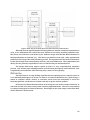
Figure III.I: Top Level System Design .......................................................................................... 22
Figure III.II: General Stereoscopic Camera Implementation ....................................................... 23
Figure III.III: Correspondence between Left and Right Images ................................................... 23
Figure III.IV: Euler angles with respect to the axes of an airplane ............................................... 24
Figure III.V: Top level flow chart of feature detector and matcher .............................................. 25
Figure III.VI: Sample image from camera before filtering ........................................................... 26
Figure III.VII: The horizontal and vertical results of the Sobel Operator ...................................... 26
Figure III.VIII: Output from blob filter ......................................................................................... 27
Figure III.IX: Circular Matching ................................................................................................... 28
Figure III.X: State and Measurement Vectors .............................................................................. 29
Figure III.XI: Observation vs. Estimation Matrix .......................................................................... 29
Figure III.XII: State Transition Matrix ........................................................................................... 30
Figure III.XIII: Dynamic Equations ............................................................................................... 30
Figure III.XIV: a priori state ......................................................................................................... 31
Figure III.XV: a posteriori state .................................................................................................... 31
Figure III.XVI: Axis Definition ...................................................................................................... 32
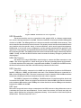
Figure III.XVII: Power Management block diagram .................................................................... 34
Figure III.XVIII: Efficiency of 3.3 V regulator (left) and 5.0 V regulator (right) ............................ 34
VII
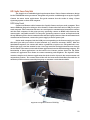
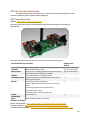
Figure IV.I: Top level system implementation ............................................................................. 37
Figure IV.II: Capella Stereo Vision Camera Reference Design.................................................... 38
Figure IV.III: GStreamer host pipeline flow diagram ................................................................... 39
Figure IV.IV: GStreamer receiver pipeline flow diagram ............................................................ 40
Figure IV.V: ADIS16375 IMU and prototype interface board ....................................................... 40
Figure IV.VI: ADIS IMU frame of reference .................................................................................. 41
Figure IV.VII: Level shifter schematic .......................................................................................... 42
Figure IV.VIII: Ninety degree rotations about Z axis ................................................................... 43
Figure IV.IX: Extended Kalman Filter flow chart .......................................................................... 45
Figure IV.X: XBee Radio and USB Interface ................................................................................. 46
Figure IV.XI: Configuring the XBee Channel and PAN ID ............................................................ 47
Figure IV.XII: MATLAB Receive and Plot ..................................................................................... 47
Figure IV.XIII: OMAP5432 EVM block diagram ........................................................................... 49
Figure IV.XIV - Comparison of visual odometry running at 5 FPS (left) and 2.5 FPS (right) ......... 50
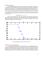
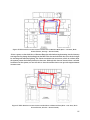
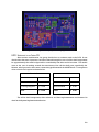
Figure V.I: Visual Odometry results on first floor of Atwater Kent, running on an x86 processor 52
Figure V.II: Third floor results of visual odometry running on x86 processor .............................. 53
Figure V.III: Bias Removal-Sitting Still ......................................................................................... 54
Figure V.IV: Bias Removal-90˚ Turns ........................................................................................... 55
Figure V.V: Values of R Matrix..................................................................................................... 56
Figure V.VI: Values of Q Matrix ................................................................................................... 56
Figure V.VII: Results of sensor fusion on first floor of Atwater Kent (Blue – raw data, Red – Sensor
Fusion, Orange – Ground truth)................................................................................................... 57
Figure V.VIII: Results of sensor fusion on third floor of Atwater Kent (Blue – raw data, Red –
Sensor Fusion, Circles – Ground truth) ........................................................................................ 57
Figure V.IX: Real-time position and heading GUI ........................................................................ 58
Figure V.X: GUI Execution Time .................................................................................................. 59
Figure A.I: Capella Camera Full Setup ........................................................................................ 75
Figure A.II - Using menucofig to include FTDI drivers in kernel build ........................................ 82
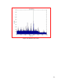
Figure A.III: X gyro data format ................................................................................................... 86
Figure A.IV: Angular rotation Z axis by parsing data in Arduino. Units of Y axis is degrees and
units of X axis is seconds. ............................................................................................................ 86
Figure A.V: FPGA based Design ................................................................................................. 87
Figure A.VI: Flowchart of Software filtering on ZedBoard ............................................................ 88
Figure A.VII: Processor Core based Design ................................................................................ 88
Figure A.VIII: Surveyor Stereo vision system .............................................................................. 89
Figure A.IX: MEGA-DCS Megapixel Digital Stereo Head ............................................................ 90
Figure A.X:nDepth Stereo Vision System..................................................................................... 91
Figure A.XI: Bumblebee 2 Stereo Vision Camera ........................................................................ 92
Figure A.XII: Scorpion 3D Stinger Camera .................................................................................. 93
Figure A.XIII: Enseno N10 Stereo Camera ................................................................................... 93
Figure A.XIV - FreeIMU PCB........................................................................................................ 95
Figure A.XV – x-IMU PCB ............................................................................................................ 96
Figure A.XVI – KVH 1750 IMU...................................................................................................... 97
Figure A.XVII - Proposed System Block Diagram Including Custom PCB .................................... 98
Figure A.XVIII - Schematic for 3.3 V regulator ............................................................................ 99
Figure A.XIX - A preliminary layout for the proposed PCB ........................................................ 100
VIII
IX
List of Tables
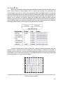
Table II.I:Number of trails N for a given sample and proportion of outliers ................................. 16
Table III.I: Peak current draw for voltage regulators ................................................................... 34
Table III.II: System current draw estimate ................................................................................... 35
Table IV.I: Capella Camera Specifications and Features ............................................................. 38
Table IV.II : Power requirements of IMU...................................................................................... 41
Table IV.III: SPI specifications for ADIS16375 and Arduino Uno .................................................. 42
Table VI.I: Design Goals and implementation status ................................................................... 60
Table A.I: Specifications and Features for Surveyor Stereo Vision System .................................. 89
Table A.II: Specifications and Features for MEGA-DCS Megapixel Digital Stereo Head .............. 90
Table A.III: Specifications and Features for nDepth Stereo Vision System ................................... 91
Table A.IV: Specifications and Features for Bumblebee 2 and Bumblebee XB3 .......................... 92
Table A.V: Specifications and Features of Scorpion 3D Stinger Camera ...................................... 93
Table A.VI: Specification and Features for Enseno N10 Stereo camera ....................................... 94
Table A.VII: Specification and Features for FreeIMU ................................................................... 95
Table A.VIII: Specification and Features for x-IMU ...................................................................... 96
Table A.IX: Specification and Features for KVH 1750 IMU ........................................................... 97
X
List of Equations
Equation II.I: Newton's force equation ........................................................................................... 4
Equation II.II: Image gradient from intensity function [11] ............................................................ 7
Equation II.III: SSD error [12]......................................................................................................... 9
Equation II.IV: First Order Taylor Series Expansion of SSD function [12] ....................................... 9
Equation II.V: Result of Taylor Series substitution to SSD error formula [12].................................. 9
Equation II.VI: Further simplification of SSD error formula [12] ..................................................... 9
Equation II.VII: SSD error as quadratic form approximation [12] ................................................... 9
Equation II.VIII: Harris Corner Detection equation [12] ............................................................... 12
Equation II.IX: Matrix H represented by weighted derivatives [12] ............................................ 12
Equation II.X: General form of integral image function [15] ........................................................ 13
Equation II.XI: World coordinates from local coordinates [17] .................................................... 15
Equation II.XII: RANSAC fundemental matrix .............................................................................. 16
Equation II.XIII: Number of RANSAC iteration ............................................................................. 16
Equations II.XIV: Linear System Definition [19] ........................................................................... 18
Equation II.XV: Noise Covariance [19] ........................................................................................ 18
Equation II.XVI: Kalman Filter [19] .............................................................................................. 18
Equation II.XVII: Relationship between image points .................................................................. 20
Equation II.XVIII: Homography matrix ........................................................................................ 20
Equation III.I: Gyroscope Rotation Matrix from Figure III.XVI ..................................................... 32
Equation III.II: Body Rotation Matrix from Figure III.XVI .............................................................. 32
Equation III.III: Body-to-Global Velocity Transformation ............................................................. 32
Equation III.IV: Body-to-Global Acceleration Transformation...................................................... 33
Equation III.V: Input Current Calculation .................................................................................... 35
Equation IV.I: IMU transformation matrix .................................................................................... 40
XI
Executive Summary
Technology for localization and tracking in outdoor environments has improved
significantly in recent years, due in great part to the advent of satellite navigation systems such as
GPS. Indoor navigation systems on the other hand have been slower to develop due to the lack of
a de facto standard method that produces accurate results. Indoor localization has potential uses
in various public indoor environments such as shopping malls, hotels, museums, airports, trains,
subways, and bus stations. With further advances in technology, indoor positioning may also find
use by emergency first responders and military personnel. The technology may also be used in
robotics, providing safe navigation for mobile robotic systems.
While satellite navigation is effective for outdoor navigation, the metallic infrastructure of
many public buildings attenuates the satellite signal strength enough to mitigate any relevant
information it might carry. Other RF based localization technologies, such as WIFI triangulation,
suffer from similar signal degradation issues. Compass based systems are ineffective due to the
magnetic interference caused by the metallic framework of larger buildings. Various technologies
for indoor localization exist, such as inertial measurement, visual odometry, LIDAR, and deadreckoning. However, these technologies by themselves often prove to be unreliable in effective
indoor localization. Visual odometry, or localization by means of camera systems, provides
accurate linear movement approximation, but tends to be inaccurate with respect to turns and
other rotational movement. Conversely, Inertial odometry, or localization with accelerometers
and gyroscopes, provides accurate rotational movement, but fails in long term linear movement
approximations due to compounded accelerometer drift associated with gravity.
This project presents a cost effective mobile design which combines both visual and
inertial odometry to perform localization within an indoor environment in real-time. The design is
intended to be placed on either a human or an otherwise mobile platform which will traverse an
indoor environment. A remote user will be able to locate the mobile platform at any given time
with respect to its starting position. The device acquires environment and motion data through a
stereoscopic camera system and an inertial measurement unit (IMU). This data is stored and
manipulated by a central processor running an embedded Linux Operating System, which
provides the core functionality to the system. The extracted coordinates are transmitted in realtime via a radio transceiver to a remote user, who can see a plot of the platform’s location and
trajectory through a custom MATLAB GUI (Graphical User Interface).
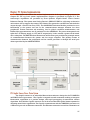
Design
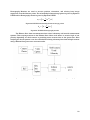
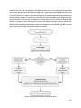
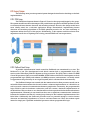
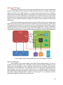
A top–level diagram of the intended design is provided below. The crux of the design lies
in the fusion of the independent visual and inertial odometry coordinates. This sensor fusion
intends to combine the strengths of the two respective odometry systems, while mitigating their
weaknesses. Once images are captured, information movement is extracted and transformed to
global coordinates. The raw acceleration and rotation data from the inertial measurement unit is
transformed to the same frame of reference as the visual odometry data. Once the data is fused,
the accurate linear movement from visual odometry can be correlated with accurate rotational
movement from the inertial measurement unit so as to more precisely reconstruct the motion of
the mobile platform.
XII
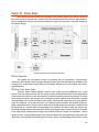
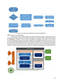
The stereoscopic camera takes a pair of left and right image frames at user-defined frame
rate. These images are run through a blob filter in order to find similar sections in the image. A
non-maximum suppression algorithm is then used to find areas of interest, or features, in these
image sections. The original images are run through a Sobel filter, which is used to create
descriptions of each of the detected features. Once features have been detected, they are matched
between respective left and right frames, as well as the image frames from the previous time step.
Circular matching is performed, in which features from the current time step’s left image are
matched along a horizontal corridor to the current time step’s right frame – and from there to the
previous time step’s right frame, then to the previous time step’s left frame, and finally back to the
current time step’s left frame. This is done so as to ensure that the same features are being matched
across time. Once features have been matched, the platform’s motion is reconstructed using
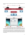
RANSAC (RAndom SAmple Consensus). RANSAC takes a small number of randomly selected,
successfully matched features, and forms a hypothesis of the system’s motion based on these
features. This hypothesis is then tested against other successfully matched features, and if enough
points fit, it is accepted as the motion of the system. However, if the test fails, a new hypothesis is
formed with a different set of points. The accuracy of the motion reconstruction ultimately depends
on the number of matched features found.
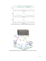
Simultaneously, the system’s acceleration and heading data is measured by the Inertial
Measurement Unit (IMU). The gyroscope data from the IMU is converted to the global frame
through a rotational matrix describing the orientation of the device relative to its starting
orientation, and then integrated to estimate Euler angles. This is combined with the accelerometer
data and converted once more to the global frame with another rotational matrix. Finally, this
global data is integrated to determine the current position of the system.
These two sets of global coordinates are weighted against each other by an Extended
Kalman Filter (EKF). The EKF estimates the current state of the system by forming and validating
hypotheses on the system state with each round of new data. The Kalman filter ideally weighs the
linear movement data from the camera and the rotational movement from the IMU strongly, while
weighing the camera rotation data and the IMU acceleration data weakly. In doing so, the design
avoids some of the pitfalls of pure vision or inertial systems, while providing better accuracy at
the expense of the complexity of sensor fusion. The Kalman filter output coordinates are
continuously transmitted to a base station, which receives the position and heading, and plots it
with respect to the initial starting position.
Conclusions
The results from this phase of the project were promising. Successful motion reconstruction
from visual odometry was obtained. Similarly, reliable heading estimations were extracted from
the inertial odometry implementation. These two sets of data were successfully fused by the
Extended Kalman filter to produce a more accurate motion reconstruction.
XIII
However, integration challenges were encountered when attempting to combine the two
technologies into a real-time, mobile platform. While the visual odometry software performed
optimally on x86 processor architectures, a successful ARM port proved to be difficult. This was in
large part due to the different set of intrinsic functions between the two architectures, but also due
to mishandling of floating point math by the ARM compiler. The intrinsic functions issues were
resolved; however the floating point errors were not able to be addressed at this time. It was also
noted that the visual odometry algorithms executed more slowly on the ARM processor despite
having comparable specifications with the x86 processor; whether this is because of the
aforementioned issues or simply due to the inherent architecture differences has yet to be
determined. Additionally, documentation and resources for the processor chosen were relatively
scarce, in large part due to the processor being new at the time. This further slowed development
time when it came to integrating the independent components with the processor.
The gyroscope contained parasitic drifts due to internal changes in temperature, changes
in acceleration, as well as inherent bias. Their removal proved to be more challenging than
originally anticipated. Regardless, much of the bias on the gyroscope was mitigated, including the
drift caused by ambient temperature changes. However, the drifts caused by unpredictable
changes in acceleration remain unresolved.
If work is continued on the project, the team recommends investigating a more powerful
choice of processor to deal with the intense computational loads required for real-time operation.
Additionally, a more robust interface between the camera and the processor would be required.
Despite these setbacks, the overall design of the system is still viable. The visual and inertial
odometry implementations were successful, as was their fusion with the EKF.
XIV
Chapter I. Introduction
Technology for localization and tracking in outdoor environments has improved
significantly in recent years, due in great part to the advent of satellite navigation systems such as
the Global Positioning System (GPS). GPS has become the de facto technology for outdoor
navigation systems, finding uses not only in military environments, but in civil and commercial
applications as well. Indoor navigation systems on the other hand have been slower to develop
due to no tangible standard method that produces optimal results.
While satellite navigation is effective for outdoor navigation, the metallic infrastructure of
many public buildings attenuates the satellite signal strength enough to mitigate any relevant
information it might carry. Additionally, the error range of GPS based systems is too large for the
resolution at which an indoor positioning system needs to perform. Other RF based technologies,
such as WIFI, suffer from the same issues. Compass based systems are ineffective due to the
magnetic interference caused by the metallic framework of larger buildings. Various technologies
for indoor localization exist, such as inertial measurement, visual odometry, LIDAR, and deadreckoning. However, these technologies by themselves often prove to be unreliable in effective
indoor localization.
Indoor navigation has potential uses in military, civil and commercial applications.
Similarly to how GPS is used to provide location directions and current position for users seeking
to traverse through an unknown outdoor environment, indoor navigation can provide
corresponding results in an enclosed environment. These include large manmade infrastructures
such as shopping malls, stadiums, and enclosed plazas, and may be even further extrapolated to
define caves and similar settings where satellite navigation would fail. With further development,
indoor navigation may be used to reliably track first responders, such as firefighters, during highrisk missions within enclosed environments. By keeping track of first responders’ locations at any
point in time, as well as any potential victims, numerous tragedies caused by logistics can be
avoided. Indoor navigation technology can likewise be beneficial for military personnel when
conducting missions in enclosed spaces.
This project explores the design and functionality of an affordable visual odometry system
for indoor use. This system will be mounted onto a moving body—such as a robot, vehicle, or
person—and will be capable of calculating in real-time the position and orientation of said body
with respect to its starting position. The design integrates several techniques so as to create a
working visual odometry system. These techniques include feature detection and matching,
RANSAC, Inertial Odometry, and an Extended Kalman Filter. This will require accurate sensors
and significant processing power in order to be implemented in real-time with little error. In order
to achieve this with an affordable system, cost-effective hardware and more efficient algorithms
were researched.
Visual odometry, or localization by means of camera systems, provides accurate linear
movement approximation, but tends to be inaccurate with respect to turns and other rotational
movement. Conversely, inertial odometry, or localization with accelerometers and gyroscopes,
provides accurate rotational movement, but fails in long term linear movement approximations
due to compounded accelerometer error. Optimal movement approximations canthus be
obtained by combining the respective strength of the two technologies, while mitigating their
weaknesses.
Visual odometry is performed through feature detection, feature matching, and motion
reconstruction. Features are detected by performing non-maximum suppression on blob filtered
images. Feature descriptors are extracted from Sobel filtered images. These descriptors are
circularly matched between current and past frames in order to efficiently determine camera
1
motion. RANSAC is then performed on the successfully matched feature in order to reconstruct the
motion of the system. Inertial odometry is performed by integrating acceleration and rotation data
so as to obtain position and heading coordinates. These coordinates, along with those obtained
from visual odometry are combined with an Extended Kalman filter which then produces a more
reasonable approximation of system motion by fusing the two data sets.
This paper outlines the research, design, and implementation of the system in question.
Initially, background information is provided on inertial and visual odometry methodology.
Afterwards, the intended system design is discussed in detail. The chosen hardware
implementation and the resulting challenges encountered are then explored. The overall results
of the independent components of the system, as well as the mobile platform as a whole are
provided. The conclusion discusses the overall performance of the system, and provides
suggestions for further improvements.
2
Chapter II. Background
This chapter provides the research performed prior to the implementation of the project.
An overview of the fundamental concepts governing the intended design will be provided.
Additionally the mathematical properties of feature detection, RANSAC, and Kalman filter
approximation will be discussed.
II.I Odometry
Odometry is the estimation of the change in location over time through the utilization of
electromechanical sensors or environment tracking. [1] Odometry systems can vary significantly
in complexity based upon the desired functionality. An example of a simple system is a typical car
odometer that measures the distance travelled by counting the number of wheel rotations and
multiplying the result by the tire circumference. The product is the distance traveled in either
imperial (miles) or metric (kilometers) units. More advanced odometry systems can provide
information including the orientation of a system with respect to an initial position, the trajectory
traveled from a starting location, and the current location of a system in relation to its initial
position. Advanced odometry systems may be implemented through a variety of methods. One
such way of tracking the orientation and movement of a system consists of measuring the forces
along the three axes as well as the angular rotation about these axes with a method known as
inertial odometry. A second method, known as visual odometry, relies instead on the change in
location of a platform with respect to static objects in the surrounding environment. The design
proposed in this paper makes use of both visual and inertial odometry to track and locate the
system.
II.I.I Inertial Based Navigation
Inertial navigation is a self-contained implementation that uses measurements provided
by accelerometers and gyroscopes to track the position and orientation of an object. It is used in
various applications including aircraft, missiles, spacecraft, and submarines. Inertial systems fall
into two categories, stable platform systems, and strap-down systems. [1]
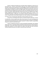
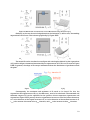
A stable platform system has the inertial system mounted on a platform which is isolated
from external rotational motion. This system uses frames which allow the platform freedom of
movement in three axes. Figure II.I and Figure II.II depict a stable platform IMU, and a stable
platform inertial measurement unit, respectively.
Figure II.I: Stable Platform IMU [1]
3
Figure II.II: Stable platform inertial navigation algorithm [1]
A strap-down system is mounted rigidly, directly onto the device, therefore the output
quantities are measured in the body frame, rather than the global frame. This requires the
gyroscopes to be integrated. [2] Figure II.III depicts a strap-down inertial navigation algorithm.
Figure II.III: Strap-down inertial navigation algorithm [1]
II.I.II Accelerometers
An accelerometer is an electromechanical device used to measure acceleration forces.
Acceleration can be expressed through Newtonian physics as:
𝑎=
𝐹
𝑚
Equation II.I: Newton's force equation
Accelerometers are generally classified under three categories, Mechanical, Solid State,
and MEMS (micro-machined silicon accelerometers). A mechanical accelerometer consists of a
mass suspended by springs. The displacement of the mass is measured giving a signal
proportional to the force acting on the mass in the input direction. By knowing the mass and the
force, the acceleration can be calculated through Newton’s equation. [1]
Figure II.IV: a) Mechanical Accelerometer [1]
b) SAW accelerometer [1]
4
A solid-state accelerometer, such as a surface acoustic wave (SAW) accelerometer,
consists of a cantilever beam with a mass attached to the end of the beam. The beam is resonated
at a particular frequency. When acceleration is applied, the beam bends, which causes the
frequency of the acoustic wave to change proportionally. The acceleration can be determined by
measuring the change in frequency.
A MEMS (micro-electrical-mechanical system) accelerometer uses the same principles as
the other two types, with the key difference being that implemented in a silicon chip, thus being
smaller lighter, and less power consuming. On the other hand, MEMS accelerometers tend to be
less accurate.
II.I.III Gyroscopes
A gyroscope is a device used for measuring and maintaining orientation using the
principles of angular momentum. Gyroscopes can generally be divided into three categories,
Mechanical, Optical, and MEMS gyroscopes. [1]
A mechanical gyroscope consists of a spinning wheel mounted upon two gimbals that
allows the wheel to rotate in three axes. The wheel will resist changes in orientation due to the
conservation of angular momentum. Thus when the gyroscope is subject to rotation, the wheel will
remain at a constant orientation whereas the angle between the gimbals will change. The angle
between the gimbals can then be read in order to determine the orientation of the device. The
main disadvantage of the gyroscopes is that they contain moving parts. Figure II.V depicts a
mechanical gyroscope system.
Figure II.V: Mechanical Gyroscope [1]
Optical Gyroscopes used the interference of a light to measure angular velocity. They
generally consist of a large coil of an optical fiber. If the sensor is rotating as two light beams are
fired on opposite sides, the beam travelling in the direction of rotation will experience a longer
path. The angle is then calculated from the phase shift introduced by the Sagnac effect.
Figure II.VI: Sagnac Effect [1]
5
As with MEMS accelerometers, MEMS gyroscopes use the same principles as the other two
types of gyroscopes, except that MEMS gyroscopes are implemented onto silicon chips. These
gyroscopes are more cost efficient and lightweight, but are generally less accurate.
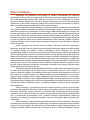
II.I.IV Mono-vision and Stereo-vision Odometry
Visual odometry is the process of using video information from one or more optical
cameras to determine the position of the system. This is accomplished by finding points of
interest, or features, in each frame or set of frames from the cameras, that are easily
distinguishable by the computer and tracking the motion of this information from one frame to the
next. Solely using feature location in the frame is not sufficient to track the motion, as this only
provides an angular relationship between the camera and the feature. To resolve this problem
multiple frames, either from the same camera over time or from two cameras simultaneously, are
used to triangulate the position of the feature.
At the highest level, visual odometry can be divided into mono- and stereo-camera
odometry. As the name implies, mono-camera systems make use of only a single camera, while
stereo-camera systems use two cameras a fixed distance apart.
Mono-vision Odometry
In order to extract depth information from a single camera, two separate frames are used
with the assumption that the camera will have moved in the time between the frames. Features
that are found in both images are then used as match points, with the camera movement used as
the baseline [3] [4].
The benefits of using only a single camera are readily apparent; there is less hardware
required reducing system size, cost and hardware complexity. Additionally, there is no need to
calibrate several cameras to work together [5] [6].
There are several drawbacks with this type of visual odometry. Camera motion is used as
a basis for the distance calculation for features. This motion is not precisely known, as it is the
unknown factor in the system.
Stereo-vision Odometry
Stereo camera odometry uses two cameras placed next to each other to determine depth
information for each frame by matching features that both cameras can see, and then watching as
the points move in space relative to the cameras as the cameras move [7]. The addition of the
second camera makes this method superior to mono-camera vision as the depth of each of the
points of interest can be found in each frame, as opposed to waiting for the camera to move to
provide perspective. Stereo visual odometry can work from just one frame to the next, or a sliding
window of frames could be used to potentially improve accuracy [8].
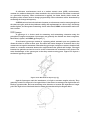
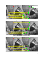
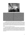
The depths of points can be found by making a ray from each camera at the angle that the
point appears to be in and using simple trigonometry to find the perpendicular distance to the
point. [9]An example of point patching between two stereo images is shown in Figure II.VII.
6
Figure II.VII - Point matching between the images from a stereo camera
Although stereo odometry requires more hardware than monocular visual odometry, it also has
increased accuracy and requires less complex computation.
II.II Feature Detection and Matching
Feature matching and detection involves the location, extraction, and matching of unique
features between two or more distinct images. Feature Detection is a general term that includes
algorithms for detecting a variety of distinct image features. These algorithms can be specialized
to detect edges, corner points, blobs, or other unique features. [10]
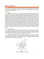
II.II.I Edge Detection
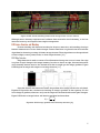
Edge detection is used to convert a Two-Dimensional image into a set of curves. An edge
is a place of rapid change in the image intensity. In order to detect an edge, discrete derivatives
of the intensity function need to be derived such that we might get the image gradient. Figure
II.VIII depicts an image with respect to its image function. [11]
Figure II.VIII: Image edge as function of intensity [11]
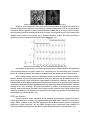
Once the discrete derivatives are found, the gradient of the image needs to be calculated.
Equation II.II provides the calculation for deriving an image’s gradient. In the equation, ∂f is the
local change in gradient, whereas x and y are the respective horizontal and vertical pixel changes.
Figure II.IX shows an image before and after the gradient has been taken.
𝜕𝑓 𝜕𝑓
∇𝑓 = [ , ]
𝜕𝑥 𝜕𝑦
Equation II.II: Image gradient from intensity function [11]
7
Figure II.IX: Image of Tiger before and after gradient [11]
However, most images will have some noise associated with the edges and must first be
smoothed. The general approach to smoothing is a using an image filter such as a Gaussian filter.
A Gaussian Filter is applied by taking a small specially crafted matrix or vector, called a kernel,
and convolving it with the intensity function of the image. The edges will occur at the peaks of the
gradient of the result (if the kernel was a Gaussian function). Figure II.X below provides a
graphical of the aforementioned smoothing implementation. [12]
Figure II.X: Smoothing process using Gaussian kernel [12]
It should be noted that due to the associative properties of differentiation. The derivative
of the intensity function no longer needs to be calculated if we are smoothing with a Gaussian
kernel. The intensity function can simply be multiplied with the intensity of the Gaussian filter.
Some common Edge detection algorithms include the Sobel method, Prewitt method,
Roberts method, Laplacian of Gaussian method, zero-cross method, and the Canny method. The
Sobel method finds edges using Sobel approximation derivatives. Similarly, the Prewitt and
Roberts methods find edges using the Prewitt and Roberts derivatives, respectively. The Laplacian
of Gaussians method finds edges by filtering an image with a Laplacian of Gaussian filter, and then
looking for the zero crossings. The zero-cross method is similar to the Laplacian of Gaussian
method, with the exception that filter on the image can be specified. The Canny method finds
edges by looking for local maxima of the gradient of the image. The gradient is calculated using
the derivative of a Gaussian filter. [13]
II.II.II Corner Detection
Corner Detection takes advantage of the minimum and maximum eigenvalues from a
matrix approximation of a summed up squared differences (SSD) error to find local corners in an
image. Three common corner detection algorithms include Harris Corner Detection, Minimum
Eigenvalue Corner Detection, and the FAST (Features from Accelerated Test) method. An
overview of Minimum Eigenvalue and Harris Corner Detection will be provided below. [13]
8
Initially, we start with a “window” (a set of pixels) W, in a known location. The window is
then shifted by an amount (u,v). Now each pixel (y, x) before and after the change is compared to
determine the change.. This can be done by summing up the squared differences (SSD) of each
pixel. This SSD defines an error, as given by Equation II.III.
𝐸(𝑢, 𝑣) =
∑ [𝐼(𝑥 + 𝑢, 𝑦 + 𝑣) − 𝐼(𝑥, 𝑦)]2
(𝑥,𝑦)∈𝑊
Equation II.III: SSD error [12]
The function I(x+u, y+v) can then be approximated through Taylor Series Expansion. The
order of the Taylor Series is proportional to the magnitude of the window’s motion. In general, a
larger motion requires a higher order Taylor series. A relatively small motion can be reasonably
approximated by a first order series. Equation II.IV shows the first order Taylor Series expansion
of the SSD function. The variables Ix and Iy are shorthand for dI/dx and dI/dy respectively.
𝜕𝐼
𝜕𝐼
𝑢
𝐼(𝑥 + 𝑢, 𝑦 + 𝑣) =
̃ 𝐼(𝑥, 𝑦) +
𝑢+
𝑣 =
̃ 𝐼(𝑥, 𝑦) + [𝐼𝑥 𝐼𝑦 ] [ ]
𝑣
𝜕𝑥
𝜕𝑦
Equation II.IV: First Order Taylor Series Expansion of SSD function [12]
The I function expression in Equation II.III can now be replaced with the Taylor expansion
derived in Equation II.IV. The result of this operation ultimately yields a much simpler equation,
as shown by Equation II.V.
𝐸(𝑢, 𝑣) =
∑ [𝐼(𝑥 + 𝑢, 𝑦 + 𝑣) − 𝐼(𝑥, 𝑦)]2 =
̃
(𝑥,𝑦)∈𝑊
2
∑ [𝐼𝑥 𝑢 + 𝐼𝑦 𝑣]
(𝑥,𝑦)∈𝑊
Equation II.V: Result of Taylor Series substitution to SSD error formula [12]
Equation II.V can be further simplified into Equation II.VI, where A is the sum of Ix2, B is the
sum of the products of Ix and Iy, and C is the sum of Iy2.
𝐴=
∑ 𝐼𝑥 2 ,
𝐵=
(𝑥,𝑦)∈𝑊
𝐸(𝑢, 𝑣) =
̃
∑ [𝐼𝑥 𝑢
∑ 𝐼𝑥 𝐼𝑦 ,
(𝑥,𝑦)∈𝑊
2
+ 𝐼𝑦 𝑣]
𝐶=
∑ 𝑦2
(𝑥,𝑦)∈𝑊
2
=
̃ 𝐴𝑢 + 2𝐵𝑢𝑣 + 𝐶𝑣 2
(𝑥,𝑦)∈𝑊
Equation II.VI: Further simplification of SSD error formula [12]
The surface SSD error E(u,v) can be locally approximated by a quadratic form (product of
matrices), as presented by Equation II.VI
𝐴 𝐵 𝑢
𝐸(𝑢, 𝑣) =
̃ [𝑢 𝑣] [
][ ]
⏟𝐵 𝐶 𝑣
𝐻
Equation II.VII: SSD error as quadratic form approximation [12]
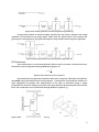
In the case of horizontal edge detection, the derivative, Ix will be zero. Thus the
expressions, A and B, found in the matrix H, will also be zero. This is shown graphically by Figure
II.XI.
9
Figure II.XI: Result of matrix H in case of Horizontal edge detection [11]
Similarly, in the case of vertical edge detection, the derivative, Iy will be zero, thus making
expressions B and C zero. This is shown graphically by Figure II.XII.
Figure II.XII: Result of matrix H in case of Vertical edge detection [11]
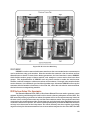
The matrix H can be visualized as an ellipse with axis lengths defined by the eigenvalues
of H, and the ellipse orientation determined by the eigenvectors of H. This can be seen in Figure
II.XIII. In general, the shape of H conveys information about the distribution of gradients around
the pixel.
Figure II.XIII: Elliptical representation of matrix H [11]
Consequently, the maximum and minimum of H needs to be found. For this, the
eigenvalues and eigenvectors of E(u,v) (the SSD error), need to be calculated. The maximum and
minimum ranges of H can be expressed as the product of their respective eigenvectors and
eigenvalues Figure II.XIV portrays how the eigenvalues/vectors are used for feature detection.
xmax is the direction of the largest increase in E, xmin is the direction of the smallest increase in E,
λmax is the amount of increase in the xmax direction, and λmin is the increase in the xmin direction.
10
Figure II.XIV: Using eigenvectors and eigenvalues in corner detection [11]
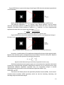
For corner detection, we want E(u,v)to be large for small shifts in all directions. Thus, we
want the minimum of the SSD error (λmin of matrix H) to be large. Figure II.XV below shows an
image, I, with corners, and the images’ maximum and minimum eigenvalues after a gradient has
been taken.
Figure II.XV: An image with its respective maximum and minimum eigenvalues [11]
Figure II.XVI visualizes the interpretation of eigenvalues for our desired functionality.
Essentially, when the maximum eigenvalue is much greater than the minimum, or vice-versa, then
an edge has been detected. However, when both the maximum and minimum eigenvalues are
large and fairly comparable in magnitude, then a corner has been detected. When both the
maximum and minimum eigenvalues are small, then a flat region has been detected (e.g. no
corner or edge).
Figure II.XVI: Interpreting eigenvalues [11]
In summary, in order to calculate corner detection, we must:
 Compute the gradient at each point in the image
 Create the H matrix from the gradient entries
 Calculate the eigenvalues
 Find the points with large responses
 Choose the point where the minimum eigenvalue is a local maximum as a feature
11
Figure II.XVII shows a point of the image I from Figure II.XV where the minimum eigenvalue is
a local maximum.
Figure II.XVII: Minimum eigenvalue as a local maximum in image gradient [11]
The minimum eigenvalue, λmin, is a variant of the “Harris Operator” used in feature
detection. The Harris Operator is given by Equation II.VIII, where the trace is the sum of the
diagonals. The Harris Corner detector is similar to λmin, however, it is less computationally
expensive because there is no square root involved.
𝜆1 𝜆2
𝑑𝑒𝑡𝑒𝑟𝑚𝑖𝑛𝑎𝑛𝑡(𝐻)
𝑓=
=
𝜆1 + 𝜆2
𝑡𝑟𝑎𝑐𝑒(𝐻)
Equation II.VIII: Harris Corner Detection equation [12]
Figure II.XVIII below shows the results of the Harris operator on the gradient of image I.
As can be seen, it is comparable to the results of the minimum eigenvalue.
Figure II.XVIII: Harris Operator as local maximum in image gradient [11]
In practice, a small window, W, is inefficient and generally does not obtain optimal results.
Instead, each derivative value is weighted based on its distance from the center pixel. Equation
II.IX provides the matrix H represented by weighted derivatives
𝐼𝑥2
𝐻 = 𝑤𝑥,𝑦 [
𝐼𝑥 𝐼𝑦
𝐼𝑥 𝐼𝑦
]
𝐼𝑦2
Equation II.IX: Matrix H represented by weighted derivatives [12]
The Harris method does not require a square root to be taken in the algorithm, and as such
is much less computationally expensive. Although the results are not as accurate as with a fully
implemented minimum eigenvalue algorithm, they are comparable enough to warrant
implementing the Harris method over the minimum eigenvalue method. [12]
II.II.III SURF and SIFT
This section will briefly discuss the Speeded-Up Robust Features (SURF), and the Scaleinvariant feature transform (SIFT) algorithms, which are used for detecting, extracting, and
matching unique features from images.
12
SIFT
The Scale-invariant feature transform, or SIFT, is a method for extracting distinctive invariant
features from images. These features can be used to perform matching between different views of
an object or scene. The advantage of SIFT is that the features are invariant (constant) with respect
to the image scale and rotation. SIFT detects key points in the image using a cascade filtering
approach that takes advantage of efficient algorithms to identify candidate locations for further
examination. The cascade filter approach has four primary steps:
1. Scale-space extrema detection: Searches over all scales and image locations.
Implemented by using a difference-of-Gaussian function to identify potential interest
points.
2. Keypoint localization: For each candidate location, a model is fit to determine location
and scale. Keypoints are then selected based upon the candidates’ measure of stability.
3. Orientation assignment: Orientations are assigned to the keypoint locations based on
local image gradient directions. Future Operations are performed on the newly
transformed image data, thus providing invariance to the transforms.
4. Keypoint descriptor: The local image gradients are measured at the selected scale in the
region around each keypoint. They are then transformed into a representation which
allows for higher levels of shape distortion and illumination modification.
SIFT generates large numbers of features that covers the image over the full range of scales
and locations. For example, an image with a size of 500x500 pixels will generate approximately
2000 stable features. For image matching and recognition, Sift features are extracted from a set of
reference images stored in a database (in the case of our design, the reference image(s) will be
the preceding image pair).The new image is matched by comparing each feature from the new
image to that of the preceding image and finding potential matching features based upon the
Euclidean distance of their feature vectors. The matching computations can be processed rapidly
through nearest-neighbor algorithms. [14]
SURF
The Speeded-Up Robust Features, or SURF, algorithm is a novel scale and rotation invariant
feature detector and descriptor. SURF claims to approximate, and at times outperform previously
proposed schemes (such as SIFT), while at the same time being able to be computed faster. The
speed and robustness of SURF is achieved by taking advantage of integral images for image
convolutions. SURF uses a Hessian matrix-based measure for detection, and a distribution based
algorithm for description. [15]
SURF initiates by selecting interest points from distinctive locations in an image, such as
corners, blobs, and T-junctions. Interest points are detected by using a basic Hessian-matrix
approximation upon an integral image. An integral image represents the sum of all pixels bits in
the input image within a rectangular region formed by the origin point and x position. Equation
II.X shows the general form of an integral image.
𝑖<𝑥 𝑖<𝑥
𝐼∑ (𝑥) = ∑ ∑ 𝐼(𝑖, 𝑗)
𝑖=0 𝑗=0
Equation II.X: General form of integral image function [15]
In the next step, SURF represents the neighborhood of every interest points through
feature vectors. The descriptor describes the distribution of intensities within the interest point
neighborhood in a similar process as SIFT, with the exception that SURF builds upon the
13
distribution of first order Haar wavelet responses rather than the gradient. The weighted Haar
responses are represented as points in a space, and the dominant orientation is estimated by
calculation the sum of the responses. This ultimately yields an orientation vector for the interest
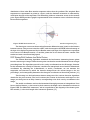
point. Figure II.XIX provides a graphic representation of the orientation vector calculation through
Haar wavelet responses.
Figure II.XIX: Orientation assignment of interest point via Haar wavelet responses [15]
The descriptor vectors are then matched between different images, based on the distance
between vectors. This process is similar to SIFT, with the exception that SURF takes advantage of
the sign of the Laplacian generated by the Hessian matrix (the sign of the Laplacian is equivalent
to the trace of the Hessian matrix) to exclude points that do not share the same contrast. This
results in a faster overall matching speed.
II.II.IV Obtaining World Coordinates from Matched Features
The Feature Detecting algorithms examined find and extract interesting feature points
from the stereoscopic images. These feature points can then be matched between the two images
preceding them. The algorithms provide local x, and y coordinates from the 2D images, however
for this information to actually be relevant, it needs to be interpolated as real world 3-dimensional
coordinates. By obtaining the 3-dimensional, or world, coordinates, we can measure the
magnitude and direction by which the features changed from the current image to the one
preceding it, and consequently determine the change in coordination of the mobile platform. [16]
The first step is to find and extract features using one of the various detection algorithms
detailed in the prior sections. The local locations (the location of the feature with respect to the
image) are then given in an N-by-2 matrix, corresponding to the local x and y coordinates in the
image.
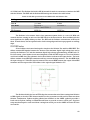
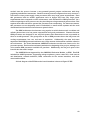
The world coordinates can then be determined through processes of triangulation. If we
have a matched feature, p¸ that is seen by both cameras, the depth can be determines as shown in
Figure II.XX. The difference between xR, and xT is equivalent to the disparity of the feature point.
The variable, f, is the focal length of the cameras in question. [17]
14
Figure II.XX: Triangulating Feature Point [17]
Thus, the next step would be to find the disparity map between the left and right images.
The disparity map will provide the depth of each pixel with respect to the cameras. The world
coordinates can then be determined if the baseline and focal length of the camera system is
known, along with the calculated disparity map. The respective equations for calculating each
world coordinate are given by Equation II.XI, where d is the disparity of the image, b is the
Vaseline, and xr, yr is the local position. Figure II.XXI provides a graphical view of the
transformation from local x,y coordinates to world XYZ coordinates by means of a disparity map.
𝑏∗𝑓
𝑥𝑅
𝑦𝑅
𝑍=
,
𝑋=𝑍 ,
𝑌=𝑍
𝑑
𝑓
𝑓
Equation II.XI: World coordinates from local coordinates [17]
Figure II.XXI: Transformation from local x,y coordinates to world XYZ coordinates [17]
Once world coordinates have been found, they can be sent to the filtering algorithms that
will remove any outliers and predict the motion of the subject based upon the coordinates.
15
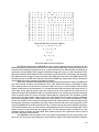
II.III RANSAC
Once features have been located in a frame, they must be matched to features in preceding
frames in order to find a hypothesis for the motion of the camera. RANSAC (Random Sample
Consensus) is an iterative method to estimate parameters of a mathematical model from a set of
observed data which contains outliers. It is used in visual odometry to remove false feature
matches [4]. Firstly, RANSAC randomly select sample of data points, s, from S and instantiates the
model from this subset [5]. Secondly, it finds set of data points Si which are within a distance
threshold t of model. Si is inlier of dataset S. Thirdly, if size of Si is greater than threshold T, model
is re-estimated using all points in Si. After N trails largest consensus set Si is selected and model is
re-estimated using all points in Si.
RANSAC computes a fundamental matrix (Equation II.XII) to identify incorrect feature
matches in stereo images, where F is the fundamental matrix and 𝜇0𝑇 and 𝜇0𝑇 are image coordinates
in pair of stereo images. [5].
𝝁𝑻𝟎 𝑭𝝁𝑻𝟎 = 𝟎
Equation II.XII: RANSAC fundemental matrix
To determine the number of iterations N, the probability of a point being an outlier needs
to be known. Equation II.XIII computes number of iterations [5].
log(1 − 𝑝)
𝑁=
log(1 − (1−∈)𝑠 )
Equation II.XIII: Number of RANSAC iteration
In the above equation, ∈ is the probability that a point is an outlier, s is the number of inliers
and N is number of trials. Table II.I gives the number of trials for a given sample size and
proportion of outliers. The algorithm was tested using the Computer Vision Toolbox in MATLAB
and the plots are show in Figure II.XXII, Figure II.XXIII and Figure II.XXIV. The minimum threshold
t was set to 10-2 for first plot and decreased in next two plots. Decreasing t increases the proportion
of outliers in the data set and gives more accurate point matches.
Table II.I:Number of trails N for a given sample and proportion of outliers
Proportion of outliers ∈
Sample size
s
2
3
4
5
6
7
8
5%
2
3
3
4
4
4
5
10%
3
4
5
6
7
8
9
20%
5
7
9
12
16
20
26
25%
6
9
13
17
24
33
44
30%
7
11
17
26
37
54
78
40%
11
19
34
57
97
163
272
50%
17
35
72
146
293
588
1177
16
Putative point matches
matchedPts1
matchedPts2
Figure II.XXII: Feature matching
Figure II.XXIII: RANSAC with threshold t=1E-4
Figure II.XXIV: RANSAC threshold t= 1E-6
17
II.IV Kalman Filter
The Kalman Filter is a widely used algorithm that uses noisy data and a dynamic model to
produce estimations of the unknown variables that describe a system’s current state. The Kalman
filter is designed to produce a recursive estimation that minimizes the mean of the square error.
This becomes very helpful in real time navigation and control of a vehicle given discrete sensor
readings. It works by approximating the state of a system in the next time step given the prior
state, the observed error, and the estimation covariance. Although the Kalman filter is designed
for linear systems, several variants of the Kalman filter have been created to describe nonlinear
systems. The linear Kalman filter relies on the dynamic equations to describe the system
functionality [18].
II.IV.I Linear Kalman Filter
The linear Kalman filter is reliable due to the fact that it provides estimated state values
that have the same average value of the true state in addition to providing the smallest possible
error variance. It achieves this by solving for the constants in Equations II.XIV that define the linear
system in which A, B, and C are matrices, k is the time index, u is a known input, y is the measured
output, x is the state of the system, and w and z are the noise [19].
State equation: 𝑥𝑘+1 = 𝐴𝑥𝑘 + 𝐵𝑢𝑘 + 𝑤𝑘
Output Equation 𝑦𝑘 = 𝐶𝑥𝑘 + 𝑧𝑘
Equations II.XIV: Linear System Definition [19]
In order to apply the Kalman filter, an assumption must be made that the process noise (w)
and the measurement noise (z) must not only be naught, but also have no correlation between
each other. This results in Equation II.XV where Sw represents the process noise covariance and
Sz represents the measurement noise covariance. In the following equations, a -1 superscript
indicates matrix inversion and a T superscript indicates matrix transposition.
𝑆𝑤 = 𝐸(𝑤𝑘 𝑤𝑘𝑇 )
𝑆𝑧 = 𝐸(𝑧𝑘 𝑧𝑘𝑇 )
Equation II.XV: Noise Covariance [19]
With this it becomes possible to solve for K, the Kalman gain, 𝑥̂, the state estimate, and P, the
estimation covariance, using Equation II.XVI.
𝐾𝑘 = (𝐴𝑃𝑘 𝐶 𝑇 + 𝑆𝑧 )−1
𝑥̂𝑘+1 = (𝐴𝑥̂𝑘 + 𝐵𝑢𝑘 ) + 𝐾𝑘 (𝑦𝑘+1 − 𝐶𝑥̂𝑘 )
𝑃𝑘+1 = 𝐴𝑃𝑘 𝐴𝑇 + 𝑆𝑤 − 𝐴𝑃𝑘 𝐶 𝑇 𝑆𝑧−1 𝐶𝑃𝑘 𝐴𝑇
Equation II.XVI: Kalman Filter [19]
II.IV.II Nonlinear Kalman Filter
Nonlinear systems are systems that cannot be described by linear equations but instead
by sets of dynamic equations. Our project requires the application of a nonlinear Kalman filter for
estimating the position of the system by analyzing the change in position of matched points from
multiple frames of our camera. There are multiple types of nonlinear Kalman Filters that each try
to reduce the error of each measurement. One such nonlinear filter is the extended Kalman filter
which uses a first-order linear approximation of the non-linear system to get an estimation of the
state variables [20]. Due to this linear approximation, the Extended Kalman filter often provides
18
error prone results and can even diverge from the true state. The unscented Kalman filter (UKF) is
a derivative-free alternative to the Extended Kalman Filter (EKF).
II.V Existing Systems
This section discusses different visual odometry systems currently available or being
researched. The first system studied was the Atlas sensor head. Atlas is a bipedal humanoid robot
developed by Boston Dynamics with funding and oversight from Defense Advanced Research
Projects Agency (DARPA). The robot is 6 feet tall and is designed for a variety of search and rescue
tasks. Atlas includes a sensory 'head' built by Carnegie Robotics which features a sophisticated
range of sensors, including a pair of stereo cameras, to give robot the 3D awareness of its
surroundings. The sensor head has an on-board processor that implements stereo algorithms that
transforms left and right images into 3D depth maps at 15 FPS. Figure II.XXV shows depth maps
generated by the sensor head. The stereovision system has a depth resolution of ±0.31 mm at 1
m and ±30 mm at 10 meters [21].
Figure II.XXV: 3D depth maps generated by Atlas sensor head[23]
Other than Atlas sensor head, the group looked into visual odometry papers presented at
IEEE conferences and proceedings of the IXth Robotic Science and Systems. Visual odometry has
widespread applications in different areas of engineering including tracking first respondents,
autonomous quadcopters and autonomous underwater vehicles. Odometry has complex problems
such as human bounce, low baseline to depth ratios and noisy data. A research group from Sarnoff
Corp. Princeton, New Jersey has developed a human wearable system with two pairs of forward
and backward looking stereo cameras together with an IMU [2]. The group has developed an
algorithm that can run in real time with 15 Hz update rate on a dual core 2 GHz laptop PC and
accurately estimate local pose and act as a front end input to the SLAM algorithm. Data from SLAM
and the IMU are integrated using an Extended Kalman filter to predict the most accurate location
coordinates. Figure II.XXVI shows block diagram of the odometry system. This method provides
more accurate results in situations when cameras fail to provide sufficient features because of poor
illumination or non-textured scenes. Figure II.XXVII shows angular velocity results from Visual
odometry (red), an IMU (blue) and a Kalman filter( green). As seen in the figure, Kalman filter
follows visual odometry measurements for all frames except for frame 2100 when the stereo
odometry result is inaccurate. Similar to the visual odometry system developed at Princeton, a
research group from the Electrical Engineering department at the University of Texas, Dallas,
created an odometry system that fuses data from an IMU, wheel encoders and stereo vision system
to improve accuracy of location coordinates [4]. Figure II.XXVIII shows translation and rotational
motion of camera frame. In the figure, Fb is the moving frame of reference, Fb* is the static frame
of reference i.e. pose at time t=0, T is the translational motion vector, R is the rotational motion
vector, m1 is the coordinates of the feature point in the moving frame of reference and m1* is the
coordinates of the feature point in the static frame of reference. Discrete and continuous
19
Homography Matrices are used to recover position, orientation, and velocity from image
sequences of tracked feature points. The relationship between image points is given by Equation
II.XVII and the Homography matrix is given by Equation II.XVIII.
𝑚𝑗 = (𝑅 +
1
𝑇𝑛∗ 𝑇 ) 𝑚∗𝑗
𝑑∗
Equation II.XVII: Relationship between image points
𝐻𝑑 = (𝑅 +
1
𝑇𝑛∗ 𝑇 )
𝑑∗
Equation II.XVIII: Homography matrix
The Kalman filter fuses measurements from visual odometry and inertial measurement
systems. Time varying matrices in the Kalman filter allows each sensor to receive high or low
priority depending on which sensor is providing more accurate data at the given time. After
studying the above systems it can be concluded that fusing odometry data from multiple sensors
using a Kalman filter gives more accurate results.
Figure II.XXVI: Flow diagram for multi camera odometry and IMU integration [22]
20
Figure II.XXVII: Results from SLAM, IMU and Kalman filter [22]
Figure II.XXVIII: Translation and rotational motion of camera frame [23]
21
Chapter III. System Design
This chapter will discuss the overall design of the mobile system. The design consists of
five major parts, Data Acquisition, Feature Detection and Matching, Kalman Filter approximation,
Power management and the top level User Interface. Figure III.I provides a top level diagram of
the system design.
Figure III.I: Top Level System Design
III.I Data Acquisition
The system has two primary means of acquiring data for localization. A stereoscopic
camera is used to bring in sets of image frames for feature detection and matching. An IMU is used
to support the output of the camera data by providing a different set of acceleration and rotation
approximations.
III.I.I Stereo Vision Camera System
A Stereo Vision Camera System consists of two image sensors configured onto a base
board in left and right positions. The two image sensors work simultaneously and independently
of one another. As such, for each discrete time constant the system produces two images, one from
each respective sensor. The images are a rectangular matrix of pixels, with the number of pixels
corresponding to the overall resolution of the image. The pixel bits control the color of the specific
pixel. For example, a 3 bit pixel will have 8 (23) distinct colors available. The number of bits per
pixel is dependent on the image sensor. These left and right images will ideally be identical with
the exception of a central offset corresponding to the baseline. In other words, the pixels of the
left image starting from the left edge and traversing the length of the baseline, as well as the pixels
of the right image starting from the right edge and traversing the length of the baseline, will be
unique to their corresponding images. The pixels not within the aforementioned range will have
equivalent correspondence between the two images. These corresponding pixels will be locally
22
shifted by the length of the baseline. Figure III.III provides a graphical representation of this
property.
Figure III.II: General Stereoscopic Camera Implementation
Figure III.III: Correspondence between Left and Right Images
This local shift of equivalent pixels between the left and right image frames is the
fundamental property that allows for depth, or Z-vector, calculations to be later produced. By
comparing the equivalent pixel movements from the frames of the next discrete time constant, the
overall movement of the camera system can be approximated within its local frame. A
stereoscopic camera system will usually have to calibrate the two frames before any processing
can be done. The calibration aligns the frames such that they fall within the same horizontal axis.
The calibration also serves to remove image distortion due to warping, and find the parameters of
the camera pairs.
23
The raw output of the Stereoscopic camera system is then encoded and compressed as
either a pair of bitmap (BMP) or JPEG images. The bitmap compression is lossless (the integrity of
the data remains the same), but the data set size is much larger. On the other hand, the JPEG
compression loses some information, but has a much smaller data set size. In either case, the
image pairs can be opened up in software as an array. The pixels can then be processed and
manipulated on the bitwise level.
III.I.II Inertial Measurement Unit
The IMU used in the system has two sensors – an accelerometer and a gyroscope to collect
acceleration and angular velocity measurements. Accelerometers measure inertial forces, or the
forces (and hence acceleration) that is directed in the opposite direction from the acceleration
vector. For example, if the accelerometer is sitting idle on the table, with positive Z axis pointing
downwards, then Z axis acceleration will be -1g. The accelerometer data consists of x, y, and z
measurements that can be used to calculate velocity and position through integration. The
gyroscope data consists of the change in roll (φ), pitch (θ), and yaw (ψ) which is the angle of
rotation about the X,Y and Z axes respectively as shown in Figure III.IV. The angular velocity,
similarly, can be used to track the angular heading of the system. The IMU sensors output an
analog voltage proportional to the sensed acceleration and angular velocity that is converted to a
digital value using an Analog to Digital Converter. IMU datasheets have conversion factors to
convert digital values from the ADC to acceleration values in meters per second squared or
degrees per second.
Gyroscopes have static bias which is the signal output from gyro when it is not experiencing any
rotation. Gyroscopes also have bias that varies with temperature and time. The variation of bias
over time is called bias drift. Gyroscopes provide reasonable estimations of turns over a short
period of time. However the position computed using accelerometer data drifts very quickly due
the cubing of measurement error. MEMS IMUs have separate registers to store accelerometer and
gyroscope data. The processor is used to communicate with the IMU to read in measurements from
the registers through digital interfaces like SPI or I2C. This data from the IMU is fused with velocity
estimations from the visual odometry subsystem in the Kalman filter. Sensor fusion with IMU data
makes the visual odometry results more robust.
Figure III.IV: Euler angles with respect to the axes of an airplane
III.II Feature Detection and Matching Algorithm
The core of the visual odometry process is the feature detector and matcher. This section
of code processes raw images into a set of points of interest that are matched between left and
right frame pairs and between subsequent frames. These points, known as features, can then be
used to reconstruct the motion of the camera. Figure III.V provides a top level view of the feature
detector and matcher.
24
Figure III.V: Top level flow chart of feature detector and matcher
Although the team experimented with writing detector, matcher and motion reconstruction
code, it was determined that it would be more efficient to use freely available published code.
The library used, Libviso2, was written by Dr. Andreas Geiger from the Max Planck Institute for
Intelligent Systems in Germany [10]. This library provided the team with a fully implemented
platform for each step of the visual odometry process. The algorithm used had several similarities
to what had already been researched by the team, with some differences. The components of the
library that are primarily responsible for the core functionality are discussed below.
The library takes many steps to speed up what is a very computationally expensive
process. One of these steps is finding features and calculating descriptors at half resolution. This
is significantly more efficient, while incurring only a minor accuracy penalty.
III.II.I Sobel Filter
The Sobel filter is an edge finding algorithm that is frequently used in computer vision as
it can efficiently find edges in an image. In order to calculate the Sobel filter for a given image, a
matrix of constants, called a kernel, is convolved across each row horizontally to create the
horizontal gradient, and down each column vertically to get the vertical gradient.
In Libviso2, the Sobel-filtered versions of the image are not used for feature detection, as
was done in some of the team’s early visual odometry implementations. Instead, it is used solely
to construct descriptors for detected features. An example of the actual output of the Sobel filter
used in Libviso2 is shown below.
25
Figure III.VI: Sample image from camera before filtering
Figure III.VII: The horizontal and vertical results of the Sobel Operator
The output consists of two different images: one representing the horizontal gradient and
one representing the vertical gradient. For applications that are intended to be directly used by
people, such as edge filters in photo manipulation software, these two images can be combined
into one that includes both horizontal and vertical edges. For the creation of descriptors however,
the two are kept separate. The descriptors are a representation of the pixels surrounding a feature
that are compared to the descriptors of other features determine if the two features are the same
object.
III.II.II Feature Detection Using Non-Maximum Suppression
Non-maximum suppression is an algorithm that thins edges in a processed image by
setting pixels in a given range to zero if they are not the highest valued pixel. This algorithm was
used to find the local maximums, which were then used as features. The images sent to the nonmaximum suppression algorithm were first run through a blob filter, which has the effect of forcing
similar areas in an image to the same color, creating sharp gradients where different areas touch.
The output of the blob filter on the image used above for the Sobel filter is demonstrated below in
Figure III.VIII.
26
Figure III.VIII: Output from blob filter
This processed image allows non-maximum suppression to easily bring out edges and
corners, which are then used as feature points. Descriptors of these features are then created
using the Sobel filtered images.
III.II.III Matching
Matching is done by comparing the descriptor of each feature with that of every other
feature. Features that are the same will have similar descriptors.
Libviso2 uses circular matching, where instead of matching features between
corresponding left and right frames and then matching then to one of the previous frames, each
feature from a given frame is tracked across each of the other four frames in a set. This is shown
in the diagram below. First, in Step 1, a feature is matched from the previous left frame to the
previous right frame. This search can be constrained to a narrow horizontal corridor, as matches
between stereo frames on a calibrated camera will be perfectly horizontal to each other. Next,
the match is then matched to the current right frame. In order to minimize the time it takes to find
the matching feature, information about the motion of the camera is used to find where the feature
is most likely, and that area is searched first. The feature from the current right frame is then
matched to the current left frame, again along a narrow horizontal corridor. Finally this feature is
matched to the previous left frame, completing a circle through all of the current set of four frames.
If the feature is matched back to the same feature that was used initially, the match is good, as the
feature can be seen in each frame so it can be used to reconstruct motion. This process is shown
in Figure III.IX.
27
Figure III.IX: Circular Matching
III.II.IV RANSAC
RANSAC is used to remove bad feature matches so that a successful motion reconstruction
can be made from only good matches. After the matcher has returned a list of matches and has
thinned them out based on some basic density parameters, the list of matches is sent to RANSAC
which builds random groups of these matches, and attempts to create motion data from these
groups. This implementation of RANSAC uses only three matches to make the initial motion
estimate, and then attempts to add more matches to this estimate. If enough other matches fit this
motion estimate, it is considered good and the algorithm stops. Otherwise RANSAC will run up the
maximum allowed number of iterations, in this case 200, and at the end take the motion estimate
that had the most corresponding matches.
III.III Non-Linear Kalman Filter Approximation
The Extended Kalman Filter (EKF) or Non-Linear Kalman Filter was used to generate a state
estimate by fusing and filtering data from both the visual odometry subsystem and the IMU. The
EKF started by making a prediction of where the system will be in the current time step based off
the state vector of the previous time step and the state transition matrix. This prediction was then
compared to the measurements of the current time step and calculated using the Kalman gain and
covariance matrix of the system. The visual odometry subsystem provided the EKF with the linear
velocity in the three axes of the body-frame. The visual odometry was also capable of providing
angular velocity but this measurement is less accurate when compared to that of the IMU. The IMU
28
provides the EKF with linear acceleration and angular velocity, both in the body frame of
reference. With these several sensor measurements, predictions become much more accurate,
despite the low sampling rate of the visual odometry subsystem. More accurate predictions result
in more effective noise removal and therefor closer estimations of the systems true movement.
Listed below are the different equations, matrices, and vectors needed for the EKF. The
subset for each variable corresponds to the x, y, or z component of that variable. Px is the position
in the x direction. vx is the velocity in the x direction. ax is the acceleration in the x direction. θx is
the angle about the x-axis. 𝜃𝑥̇ is the change in the angle about the x-axis. Figure III.XVIII shows the
state and measurement vectors. The state vector shows all of the variables that are estimated and
the measurement vector shows all of the measurements that are received from the cameras and
IMU. Figure III.XI shows the observation versus estimation matrix. This matrix compares what
information is received from the cameras and IMU to the variables that are estimated. Figure III.XII
displays the state transition matrix of the system using the dynamic equations shown in Figure
III.XIII. The time step dt in these equations and matrices is determined by the update rate of the
IMU due to its much faster sampling rate than that of the visual odometry subsystem. The dynamic
equations listed below are in terms of the x-axis but can be extended to the y and z axes.
𝑃𝑥
𝑃𝑦
𝑃𝑧
𝑣𝑥
𝑣𝑦
𝑣𝑧
𝑎𝑥
𝑎
𝑥𝑘 = 𝑎𝑦
𝑧
𝜃𝑥
𝜃𝑦
𝜃𝑧
𝜃̇𝑥
𝜃̇𝑦
[ 𝜃̇𝑧 ]
𝑦𝑘=
𝑣𝑥
𝑣𝑦
𝑣𝑧
𝑎𝑥
𝑎𝑦
𝑎𝑧
𝜃̇𝑥
𝜃̇𝑦
[ 𝜃̇𝑧 ]
Figure III.X: State and Measurement Vectors
0
0
0
0
𝐻= 0
0
0
0
[0
0
0
0
0
0
0
0
0
0
0
0
0
0
0
0
0
0
0
1
0
0
0
0
0
0
0
0
0
1
0
0
0
0
0
0
0
0
0
1
0
0
0
0
0
0
0
0
0
1
0
0
0
0
0
0
0
0
0
1
0
0
0
0
0
0
0
0
0
1
0
0
0
0
0
0
0
0
0
0
0
0
0
0
0
0
0
0
0
0
0
0
0
0
0
0
0
0
0
0
0
0
0
0
0
0
1
0
0
0
0
0
0
0
0
0
1
0
0
0
0
0
0
0
0
0
1]
Figure III.XI: Observation vs. Estimation Matrix
29
1
0
0
0
0
0
0
𝐹= 0
0
0
0
0
0
0
[0
0
1
0
0
0
0
0
0
0
0
0
0
0
0
0
0
0
1
0
0
0
0
0
0
0
0
0
0
0
0
𝑑𝑡 0 0
0 𝑑𝑡 0
0 0 𝑑𝑡
1 0 0
0 1 0
0 0 1
0 0 0
0 0 0
0 0 0
0 0 0
0 0 0
0 0 0
0 0 0
0 0 0
0 0 0
. 5𝑑𝑡 2 0 0 0 0 0 0 0 0
0 . 5𝑑𝑡 2 0 0 0 0 0 0 0
0 0 . 5𝑑𝑡 2 0 0 0 0 0 0
𝑑𝑡 0 0 0 0 0 0 0 0
0 𝑑𝑡 0 0 0 0 0 0 0
0 0 𝑑𝑡 0 0 0 0 0 0
1 0 0 0 0 0
0 0 0
0 1 0 0 0 0
0 0 0
0 0 1 0 0 0
0 0 0
0 0 0 1 0 0 𝑑𝑡 0 0
0 0 0 0 1 0 0 𝑑𝑡 0
0 0 0 0 0 1 0 0 𝑑𝑡
0 0 0 0 0 0
1 0 0
0 0 0 0 0 0
0 1 0
0 0 0 0 0 0
0 0 1 ]
Figure III.XII: State Transition Matrix
𝑃̂𝑥 = 𝑃𝑥 + 𝑣𝑥 ∗ 𝑑𝑡 + 0.5 ∗ 𝑎𝑥 ∗ 𝑑𝑡 2
𝑣̂𝑥 = 𝑣𝑥 + 𝑎𝑥 ∗ 𝑑𝑡
𝑎̂𝑥 = 𝑎𝑥
𝜃̂𝑥 = 𝜃𝑥 + 𝜃̇𝑥
𝜃̂̇𝑥 = 𝜃̇𝑥
Figure III.XIII: Dynamic Equations
The EKF was first written in MATLAB due to the ease of plotting data and running tests. The
MATLAB starts by loading in the data from the cameras and the IMU. The cameras provide position
in meters and heading in degrees for the x, y, and z directions. The IMU provides acceleration in
meters per second squared and change in heading in degrees in the x, y, and z directions. The z
direction is forward and backward. The y direction is up and down. The x direction is left and right.
The buffer size and change in time are set next. The buffer size is the size of the IMU data set. The
variable dt is set to the IMU time difference because the IMU and camera data needs to be synced
and the IMU has a faster sampling rate than the camera.
Next, state variables are initialized using the first data points from the camera and IMU data
sets. The position variables are initialized to zero. The initial state vector is initialized to these
initial state variables and the initial covariance matrix is set up to a 15x15 identity matrix. Next,
matrix xk and vector xp are initialized. xk is a matrix that stores the iterations of the state vector. xp
is the state vector after the predict state also called a priori. One iteration of xk (state vector) is
depicted in Figure III.X. Matrix Pk and Pp are initialized next. Pk is a matrix that stores the iterations
of the covariance matrix. Pp is the covariance matrix after the a priori state. The variables Q and R
are set next. Q is the matrix for the process noise. This matrix only has values along the diagonal
and zeroes everywhere else. These values can range from 0.1 to 0.2 and are adjusted to help
correct the output. R is the matrix for measurement noise. This matrix also only has values along
the diagonal and zeroes everywhere else. The values are based off of the noise properties for the
camera and IMU based on their data sheets. The yk matrix is set up next, which holds the iterations
of the measurement vector and one iteration (measurement vector) is shown in Figure III.X. The H
matrix is then set up which tells the system what are the observed states and which are the
estimated states as shown in Figure III.XI. This matrix is used in the a posteriori state to choose
only the values that are measured.
The MATLAB code then enters a for loop, which runs through all of the data points in the
data sets. The loop starts by updating the state transition matrix. This matrix holds the dynamic
30
equations used to predict the next state. These equations are nonlinear because the modeled
system itself is nonlinear. These dynamic equations are shown in Figure III.XIII and the state
transition matrix is shown in Figure III.XII.
%Predict / a priori
%state equation
xp = F*xk(:,i-1);
%covariance of the estimation error
Pp = (F*Pk(:,:,i-1)*F') + Q;
Figure III.XIV: a priori state
The next state is the predict state, also called a priori. This state predicts where the system
will be in the next iteration. The MATLAB code is shown in Figure III.XIV. The first equation is the
state equation, which makes the prediction. The second equation is used to update the covariance
matrix. The covariance matrix is used to tell the Kalman Filter how much confidence there is in the
specific value. These numbers range from zero to one with zero being very confident and one
being not confident.
Next is the update state also called a posteriori. This state corrects the values predicted in
the a priori using the measurement data taken in from the cameras and IMU. Figure III.XV shows
the a posterior state. The measurement data is collected before these steps. The Kalman gain is
calculated first. Then the state vector is corrected using the new measurement data. The
covariance matrix is also corrected using the new measurement data. The MATLAB code ends by
plotting the position data of the state vector.
Figure III.XV: a posteriori state
III.III.I Data Transformation
The accelerometer and gyroscope within the IMU are integral parts of this project. Like the
camera, they assist in the tracking of position and orientation. They are able to do this in much less
time with much less complicated processing than the camera system. Both of them serve as inputs
to the Kalman Filter by providing the angular rate of change and linear acceleration. Before they
can be processed by the Kalman Filter, they must be translated from the local, or body frame, to
the global frame. This is accomplished by keeping track of the angular orientation of the system
in relation to the global axes. The angular orientation can be described by the three Euler angles
of roll, pitch, and yaw as shown in Figure III.XVI. By converting the accelerometer measurements
to the global frame, gravity can be removed by subtracting 9.8 m/s2 from the y-axis acceleration.
31
Figure III.XVI: Axis Definition
Gyroscope and Accelerometer Rotation Matrix
The rotation of a body in 3D space is represented using Euler angles convention, in which
φ is the rotation of the system about the global z-axis, θ is the rotation about the x-axis and φ is the
rotation about the y-axis. The gyro rates are transformed to global frame using the following
rotational matrix for Euler angle rates.
0
𝜓̇
[ 𝜃̇ ] = [0
1
𝜑̇
𝑐𝑜𝑠𝜑
𝑠𝑖𝑛𝜑/𝑐𝑜𝑠𝜃
𝑠𝑖𝑛𝜑 ∗ 𝑡𝑎𝑛𝜃
−𝑠𝑖𝑛𝜑
𝜓̇′
𝑐𝑜𝑠𝜑/𝑐𝑜𝑠𝜃 ] ∗ [ 𝜃̇ ′ ]
𝑐𝑜𝑠𝜑 ∗ tan 𝜃
𝜑̇ ′
Equation III.I: Gyroscope Rotation Matrix from Figure III.XVI
Because the above equation requires the global orientation in order to calculate the global
change in orientation, a previous calculation or estimation of heading is required. In our design,
the predicted heading produced within the Kalman filter was used.
Likewise, the acceleration component in each global dimension is computed from a
rotation matrix described in Equation III.IV and Equation III.II. The headings used to compute the
Body Rotation Matrix can either be calculated by integrating the change in each heading
calculated in Equation III.I or by using the predicted heading of the Kalman filter. In order to stay
consistent with the calculation of the global angular velocities, the predicted heading from the
Kalman filter is used.
cos(𝜃) cos(𝜓)
𝐶𝑛𝑏 = [ cos(𝜃) sin(𝜓)
−sin(𝜃)
− cos(𝜙) sin(𝜓) + sin(ϕ) sin(θ)cos(𝜓)
cos(𝜙) cos(𝜓) + sin(𝜙) sin(𝜃) cos(𝜓)
sin(𝜙) cos(𝜃)
sin(𝜙) sin(𝜓) + cos(𝜙) sin(𝜃) cos(𝜓)
− sin(𝜙) cos(𝜓) + cos(𝜙) sin(𝜃) sin(𝜓)]
cos(𝜙) cos(𝜃)
Equation III.II: Body Rotation Matrix from Figure III.XVI
𝑣𝑧
[𝑣𝑥 ]
𝑣𝑦
=
𝑔𝑙𝑜𝑏𝑎𝑙
𝐶𝑛𝑏
𝑣𝑧
∗ [𝑣𝑥 ]
𝑣𝑦
𝑏𝑜𝑑𝑦
Equation III.III: Body-to-Global Velocity Transformation
32
𝑎𝑧
[ 𝑎𝑥 ]
𝑎𝑦
=
𝑔𝑙𝑜𝑏𝑎𝑙
𝐶𝑛𝑏
𝑎𝑧
∗ [ 𝑎𝑥 ]
𝑎𝑦
𝑏𝑜𝑑𝑦
Equation III.IV: Body-to-Global Acceleration Transformation
III.III.II Noise and Data Weighting
The weighting of the data allows the system to decide which input data it should rely on
more over others. Weighting of the data occurs in the covariance matrix. These values range from
zero to one. The closer the values are to zero the more confident the EKF is in that value. The EKF
then uses equations to appropriately change the covariance matrix to fit the desired need of the
system. Covariance matrices are usually initialized to be an identity matrix.
There will always be white Gaussian noise associated with data coming from the sensors.
The Q and R noise matrices are used to best understand this noise. The Q matrix, called process
noise, is used to represent the noise that is introduced when predicting the next state. The R matrix,
called measurement noise, is used to represent the noise produced by the sensors of the system.
To find the appropriate values for these matrices, our system was left sitting still for a fixed period
of time. This data set consisted of measurements for all of the different inputs of the system. The
measurements of velocity, acceleration, and angular velocity had a mean value of zero. The
standard deviation was taken on each of these inputs. These standard deviations were then
squared and used as the values for the R matrix to best model the noise coming from the sensors
of the system. The Q matrix uses these values for the measured variables and deriving the values
for the unmeasured variables.
III.IV Power Management
There are several different voltage levels required in the system. The OMAP EVM has
internal voltage regulators that accept any voltage from five to fifteen volts at one amp or less. The
Capella Camera requires five volts at one amp. As discovered in testing, the IMU needs a very
clean power supply that can support the 1.5 A transient as it turns on. To meet these requirements,
two switching regulators were chosen to supply the 3.3 V and 5 V regulated voltages for the IMU
and Capella. As the EVM would be regulating its input voltages, it was connected directly to the
unregulated input voltage. Both the XBee wireless transceiver and the Arduino would be powered
off the EVM’s 5 V USB bus power. A top level block diagram of the power management system is
shown in Figure III.XVII.
33
Figure III.XVII: Power Management block diagram
III.IV.I Switching Regulators
To speed the development process, off the shelf switching regulators were chosen. As
each regulator only had to power one device, determining max current draw was relatively
straight forward. The peak current requirements for each of the regulators are shown below.
Table III.I: Peak current draw for voltage regulators
3.3 V Regulator
IMU
1.5 A
5.0 V Regulator
Capella Camera
1A
It was decided to use D15V35F5S3 switching regulator modules from Pololu, a
manufacturer of parts for hobby robotics. The regulator has a small form factor, can be plugged
into a protoboard, and has a selectable output voltage to either 3.3 V or 5 V. Because of this, the
same type of regulator could be used for both supplies. The regulators have a high efficiency,
approximately 90% for both with an input voltage of 7.2 V and under the given load conditions.
The efficiency curves for each of the regulators are shown below in Figure III.XVIII. The regulators
were mounted on a custom protoboard which provided them with terminals to connect to the
various subsystems that required regulated voltages.
Figure III.XVIII: Efficiency of 3.3 V regulator (left) and 5.0 V regulator (right)
34
III.IV.II Battery
To allow for mobility, the system needed to be powered by a battery. The highest input
voltage allowable was 15 V, limited by the voltage regulator on the EVM. The minimum voltage
allowable was 6.5 V, limited by the dropout voltage of the 5 V regulator. Given these voltage
requirements, a 7.2 V nickel-metal hydrate, or NI-MH battery was a chosen. The necessary
capacity for the battery was then determined by estimating the current draw of the system for a
typical case. Although all of the other current draw analysis was done for the worst case, that does
not give a reasonable estimation for battery life, as most of the components do not run at their
worst case current draw for the entire time. This is especially true for the IMU, which has a startup
transient of 1.5 A, but only draws 200 mA during regular operation. To determine current draw
from the regulators, the following equation was used.
𝐼𝑖𝑛 =
𝐼𝑜𝑢𝑡 ⋅ 𝑉𝑜𝑢𝑡
𝐸 ⋅ 𝑉𝑖𝑛
Equation III.V: Input Current Calculation
In the above equation, E is the efficiency of the regulator, in this case estimated at 85%. The
current estimate for the typical case is then shown below.
Table III.II: System current draw estimate
Device
OMAP EVM
3.3 V Regulator
5 V Regulator
Total
Current Draw (A)
0.8
0.1
0.6
1.5
III.IV.III Safety Measurements
In order to prevent the battery from being damaged in the event of a short circuit, a fuse
was placed in the positive power supply line. The fuse is rated for 5 A, to allow for regular
operation, which can reach two amps, and also allow for enough overhead for startup transients
or other short spikes in power usage. Additionally, each of the Pololu voltage regulators had a
built in over-current shutdown feature, which would cause them to turn off in the event of a current
draw beyond their capacity.
III.V User Interface
The system must be capable of displaying or communicating the tracked position and
orientation of the system. An initial design implemented an LCD on the system that displayed a
numerical representation of the position and heading. The group decided this setup would be too
costly and add more work and possible problems to the project. Instead our design implements a
wireless transceiver that can be used to transmit the information to a second system that can
display or process the information in any way the user wishes.
III.V.I Wireless Radio Communication
The design implements a transceiver that transmits the data from the mobile system as a
frame as well as a transceiver that reads in the frames to a computer. The frames include the x, y,
and z positions as well as the pitch, yaw and roll. The frames have the following comma delimited
structure:
[x-position], [y-position], [z-position], [pitch], [yaw], [roll]
35
Wireless transceivers enable data to be transmitted in both directions, allowing commands
to be sent to the system. These commands may include asking the system to report its position,
zero its position and heading, and anything else deemed important. The system could also be
implemented in a spoke-hub structure, in which multiple odometry systems report their locations
and orientations to a central receiver. This would be very useful for search and rescue and military
operations.
36
Chapter IV. System Implementation
This chapter will discuss the realized implementation of the system design presented in
Chapter III. The top level system implementation diagram is provided by Figure IV.I. The
stereoscopic capabilities are provided by E-con System’s Capella Stereo Vision Camera
Reference Design. The system uses Analog Device’s ADIS16375 IMU for collecting acceleration
and rotation data to support the camera. The Arduino Uno parses the raw IMU data and feeds the
output through a Virtual Com Port (VCP). The OMAP5432 Evaluation Module provides the core
functionality to the system and acts as the communications manager between the other
peripherals. Feature detection and matching, local to global coordinate transformation, and
Kalman filter approximations are all performed on the OMAP5432. The power management unit
splits the 7.2V battery supply to 3.3V and 5V respectively. It also contains a power on/off switch
and a safety fuse. The XBee Wireless Transceiver and Receiver pair provides the principal means
of communications between the system and the target computer. The primary means of
communication between the peripherals and the central processor is through the serial port
drivers provided by the OMAP5432 EVM.
Figure IV.I: Top level system implementation
IV.I Capella Camera Stereo Vision System
The Capella camera is an embedded Stereovision reference design for the TI OMAP35x
and DM37x line of processors. The Capella is targeted towards customers seeking to integrate
Stereovision capabilities in a product design, and rapid prototyping of stereovision camera
algorithms. At $1,299 the Capella camera is one of the more affordable global shutter systems for
obtaining stereovision capabilities. The Capella communicates with the OMAP5432 processor via
a USB serial port and an Ethernet connection. The Ethernet connection is used for transmission of
37
the video stream from the camera to the processor. The serial port is used to run the initialization
scripts on the camera processor. The Capella comes with a preinstalled Linux kernel containing
the camera drivers and various camera applications. The Linux kernel also provides the potential
for extending the cameras functionality to meet our requirements. Refer to Appendix A.III for
documentation on setting up and using the camera.
Figure IV.II: Capella Stereo Vision Camera Reference Design
IV.I.I Specifications
Table IV.I provides the specifications for the Capella Camera. The primary benefits of the
Capella is the fairly low voltage power requirement as well as the Linux 2.6.35 kernel which allows
for streamlined communication between the Overo processor (OMAP35x architecture) on the
camera and the OMAP5432 EVM.
Table IV.I: Capella Camera Specifications and Features
FRAME RATE
RESOLUTION
IMAGE FORMATS
LENS TYPE
BASELINE
CAMERA BOARD
CAMERA
OUTPUT FORMAT
INTERFACE
DRIVERS
SOFTWARE
POWER SUPPLY
PRICE
SPECIFICATIONS AND FEATURES
30 fps
736x480 (per camera) ,1472x480 (combined camera resolution)
8-bit greyscale format
Factory calibrated S-mount lens pair with lock-nut and S-mount
lens holder
100mm (adjustable on request)
E-CAM 9v024 Stereo
1/3” Global shutter MT9V024 image sensor
WVGA 752(H) x 480(V) (360690 pixels) sensors output
736(H)x480(V) images in 8-bit greyscale format
27 pin FPC connector to Gumstix Overo WaterSTORM COM,
HDMI-DVI cable, USB type A to Mini B cable, Ethernet port
Standard V4L2 compliant drives with associated API’S
Linux 2.6.35 kernel, OpenCV for depth measurement
5V, 1A
$1,299.00
IV.I.II File Transfer Protocol (FTP) Network
The Capella operating system came with a pre-installed FTP server with the intention of
transferring files to and from the camera. As the user does not have direct access to the SD card
containing the Capella OS file system, the FTP network is the primary means by which the user
38
can modify the Operating system. The user must first specify the IP (internet protocol) address of
the camera, at which point the receiving computer may access the camera file system with an FTP
client.
IV.I.III GStreamer Multimedia Framework
The only means of outputting the video stream externally provided natively by the Capella
Camera is through the HDMI out port. The OMAP5432 EVM processor does not contain an HDMI
in port, and as such additional functionality has to be provided to the Capella Camera. The
GStreamer Multimedia Framework is an open-source library that allows for the manipulation,
processing, and streaming of video and audio sources. Building and installing GStreamer on the
Capella camera provided the capability to stream the camera feeds to a different computer
through a local Ethernet connection. In order to do this, corresponding GStreamer pipelines are
initiated on both the host (Capella) and the receiving (OMAP5432) computers. For further detail
on building GStreamer and constructing pipelines refer to Appendix A.III.
GStreamer Streaming Host Pipeline
The GStreamer host pipeline is run on the Capella Camera. The pipeline opens the video
streams from the left and right cameras and formats the raw video as 640x480 grayscale streams
transmitting at 5 frames per second. The pipeline then gives the streams a color space and
payloads the stream for Real-time Transport Protocol (RTP) format. Finally the pipeline defines a
UDP (User Datagram Protocol) port for each stream and transmits them at the user specified IP
address. Figure IV.III provides a flow diagram of the host pipeline.
Figure IV.III: GStreamer host pipeline flow diagram
GStreamer Receiver Pipeline
The GStreamer receiver pipeline is run on the OMAP5432 EVM. This pipeline connects to
the UDP network set up by the host pipeline and opens the respective video ports. The pipeline
capabilities are based upon the verbose outputs of the host pipeline. Afterwards the video streams
are de-payloaded and converted back into the same color space. Each incoming frame is then
encoded as a JPEG image and saved into a folder to be accessed by the feature detection
algorithm. Figure IV.IV provides a flow diagram of the receiver pipeline.
39
Figure IV.IV: GStreamer receiver pipeline flow diagram
IV.II ADIS16375 IMU Interface
The ADIS16375 is a high-end IMU that has a tri-axis gyroscope with range of ±3000 degrees
per second and a tri-axis accelerometer with range of ±18 g. It was donated for the research
project by Analog Devices so the group could make use of a high quality IMU for the project
despite the high price. The IMU has a MEMS angular rate sensor, a MEMS acceleration sensor
and an embedded temperature sensor. The outputs from the sensors are written to a thirty two bit
output registers after calibration for bias which gives high precision measurement values. The
IMU module is compact and has dimensions of 44 by 47 by 14 mm. Analog Devices provided a
prototype interface board that comes with larger connectors than the connector on the IMU to
facilitate prototyping. Figure IV.V below shows the IMU and the prototype board. The following
sections describe IMU axis, SPI bus for interfacing IMU with processor and power requirements of
the IMU.
Figure IV.V: ADIS16375 IMU and prototype interface board
IV.II.I IMU Frame of Reference
The IMU coordinate axis is shown in Figure IV.VI below. The data collected using the IMU
is converted from the IMU frame of reference to the system's frame of reference using the rotational
matrix in Equation IV.I.
𝑥𝑖𝑚𝑢
0
𝑦
[ 𝑖𝑚𝑢 ] = [0
𝑧𝑖𝑚𝑢
1
1
0
0
𝑥𝑠𝑦𝑠𝑡𝑒𝑚
0
1] × [ 𝑦𝑠𝑦𝑠𝑡𝑒𝑚 ]
𝑧𝑠𝑦𝑠𝑡𝑒𝑚
0
Equation IV.I: IMU transformation matrix
40
Figure IV.VI: ADIS IMU frame of reference
IV.II.II Power Requirements
Table IV.II below shows the power requirements of the IMU and Arduino as per their
datasheet. The IMU is powered by a 7.6 V Lithium-ion-polymer battery by stepping down the
battery output to 3.3 V using a D15V35F5S3 adjustable regulator. Arduino is powered through the
OMAP EVM through a USB port. IMU- Arduino integration in the final system is shown in a block
diagram in section.
Table IV.II : Power requirements of IMU
Parameter
Operating
voltage
Power supply
current
Transient
currents
ADIS16375
3.3 V
Arduino
5V
173 mA
200 mA
1.5 A
IV.II.III SPI (Serial Peripheral Interface)
The IMU has a SPI compatible serial interface to connect it to an embedded system SPI is a
synchronous serial data link that operates in full duplex communication. SPI has four main linesslave select, serial clock, master out slave in (MOSI) and master in slave out (MISO). In the system,
the embedded processor is the master and the IMU is the slave device. The master generates the
serial clock which sets the speed of the link, initiates the data frame and selects the slave device
by setting the slave select (SS in the figure below) low.
The OMAP has four SPI modules and the OMAP EVM breakout header has pins that provide
access to SPI module 2 in the OMAP. To register the SPI slave device with the OS, the Linux kernel
requires a device tree file. The device tree is a structure of nodes and properties. Each device
connected to the CPU is represented as a node and has a compatibility property which enables
the operating system to decide which device driver to bind to a device. It was not feasible to
interface the IMU directly with the OMAP processor because the device tree file for the OMAP was
not found in the Ubuntu Linux distribution installed on the OMAP EVM. Given the time constraints
and lack of documentation on how to implement a device tree for SPI, this option was abandoned.
As a workaround we used an Arduino Uno board as a medium between the IMU and the OMAP.
The Arduino Uno is a development board based on the ATmega328. The IMU connects to the
Arduino via SPI and the IMU data is parsed in the Arduino, and printed to a serial port at baud rate
41
of 115200 baud. The Arduino has built in SPI drivers which made it convenient to interface the IMU
with the Arduino. The IMU and the Arduino SPI settings are shown in the table below.
Table IV.III: SPI specifications for ADIS16375 and Arduino Uno
Setting
SCLK
SPI Mode
Bit Sequence
ADIS 16375
Slave
≤15 MHz
SPI Mode 3
CPOL=1 and CPHA=1
MSB first
Arduino
Master
8 MHz
SPI Mode 3
MSB first
The Arduino is the master device that generates system clock at a rate of 8 MHz and
controls the data coming in and out of the IMU which is the slave device. Data is shifted with the
most significant bit (MSB) shifting out first. The IMU and the Arduino communicate in SPI mode
three. In mode three, data is captured on the clock's rising edge and data is propagated on a falling
edge.
IV.II.IV IMU Interface
A level shifter circuit was developed to interface the Arduino Uno with the ADIS IMU. The
shifter connects SPI signals between the devices. The minimum digital high voltage that can be
read by the Arduino is 3 V and the minimum digital high voltage guaranteed by the IMU is 2.4 V.
For this reason a level shifter circuit was designed to shift the IMU output to 5V so that Arduino
could read in IMU data. The schematic for the level shifter is shown in the figure below. The level
shifter consists of two NPN BJT transistors and four current limiting resistors. The first NPN shifts
the input voltage to 5 V but the signal is inverted. The second NPN reverses the output of first NPN
transistor and the output of the level shifter is the original signal shifted to 5 V.
Figure IV.VII: Level shifter schematic
The Arduino shield also has an FTDI chip that converts the serial data coming from Arduino
to USB signals so that the FTDI drivers installed on the processors could read the data sent from
Arduino. Furthermore, Python module pySerial was installed on the OMAP. pySerial provides a
back end for Python running on Windows and Linux to provide access to serial port. A python
script was developed to read serial data coming from serial port on the OMAP and save the data
in a text file.
42
IV.II.V IMU Data Transmission
In the final system implementation, the Arduino reads in data from IMU at a frequency of
100 Hz using a hardware timer with a period of 10ms. The Arduino script initializes a 16 bit internal
hardware timer called 'Timer 1'. The Interrupt Service Routine flags the interrupt from Timer 1. A
loop constantly checks for the flag and when the interrupt is flagged, a new measurement is read
from the accelerometer, gyroscope and temperature sensor in the IMU. The data is transmitted by
serial communication to the processor in the following comma delimited data format in which the
second, third, and fourth measurements are angular velocities and the last three measurements
are accelerations.
[temperature, 𝜑̇ , 𝜃̇, 𝜓̇, , 𝑎𝑧 , 𝑎𝑥 , 𝑎𝑦 ]
The plot of the integrated gyroscope measurements from the experiment is shown in the
figure below. Ninety degree turns were estimated accurately as shown in Figure IV.VIII. The plots
show that the system can read in sensor values accurately at precise time intervals to get accurate
estimation of headings from the measurements.
psi vs time
50
0
-50
psi(degrees)
-100
-150
-200
-250
-300
-350
-400
0
50
100
150
200
time(seconds)
250
300
350
400
Figure IV.VIII: Ninety degree rotations about Z axis
IV.III Kalman Filter on the ARM Platform
A C++ implementation of the EKF has been designed to run on the ARM platform using an
OpenCV matrix library. The EKF is written as a function that reads in the next measurements from
the camera and the IMU as inputs. It then goes through the a priori and a posteriori states of the
EKF using the new measurements. The EKF sets the state vector and covariance matrix as global
variables allowing them to be used for the next iteration of the EKF. The EKF function will then
43
output the state vector of the system. The position data from the state vector will then be sent over
to the XBee, which transmits the position of the system to the base station.
To get the design running on the ARM platform the correct library is needed and the cross
compiler needs to be set up. The EKF function uses matrices to store data and does matrix
manipulations to calculate better approximations of the system. To do these calculations a matrix
library is needed. Finding the correct library did pose a challenge. The first library used was
called Meschach. The documentation for the library created the illusion that it would be of use.
However, when doing initial testing some of the functions did not work properly. The functions
that were being used to set the values of the elements were not correctly inputting the data. The
functions that would manipulate the data also were not performing the calculations correctly. The
outputted data would not be correct. After looking through the library and seeing how the
functions were written, it was apparent that the functions were not written properly. Instead of
rewriting these functions and a different library was used. OpenCV had a matrix library where the
functions were written properly. After doing some basic manipulations of matrices using the
functions from OpenCV it was apparent that the functions were performing correctly. Once a
working matrix library was found the EKF was then written in C++ and tested on an x86 platform.
Once the EKF was proven to work on an x86 platform, the next challenge was to get it to
cross compile onto the ARM platform. The compiler that was used is called arm-linux-gnueabihfg++. The challenge was getting the matrix library to compile and link correctly. When building
the matrix library only a portion of the library would build and link. However, the part of the library
that is being used by the EKF was built and linked. The problem was that the compiler couldn’t
find the library. Changing where the compiler was looking for the library was tried first but it did
not work. Next, the library was rebuilt and relinked to try to connect the library to the directory
where the compiler was looking. The compiler still couldn’t find it. Finally, the library was built
and linked in its own directory and then copied over to the directory where the compiler was
looking. This finally worked and the EKF does compile for the ARM platform.
IV.III.I Design Changes
The first step of the Kalman filter is the transformation of the measurements of the visual
odometry subsystem and IMU sensor from the systems body frame of reference to the global
frame. This transformation relies heavily on the accuracy of the heading estimations and
measurements. Because we were not able to completely remove the bias introduced by changes
in acceleration within the IMU, we were not able to fully implement local-to-global transformation.
To adjust for this, we found that if the system was kept relatively flat during testing, the angles of
roll and pitch could be set to zero. This effectively equates to the local yaw of the system being the
same as the global yaw.
Because of the complications in removing the gyroscopes drift, we were unable to
implement the entire Kalman filter that was described before. Without accurate calculations of the
roll and pitch of the system, acceleration measurement became useless due to the components of
gravity present in each axis. Because the roll and pitch had to be set to zero, the systems
capabilities were very limited. Any slight change in pitch or roll resulted in inaccurate data being
recorded.
IV.III.II Extended Kalman Filter Process
Figure IV.IX below shows the overall flow chart of the different steps that the EKF takes to
produce the filtered output state. The EKF first takes in the data from the camera and the IMU. The
44
constants and all of the variables that the EKF will need, such as the state and measurement
vectors, are initialized next. The EKF then enters the a priori state were the EKF will predict the
next state of the system as well as predict the next covariance matrix. It then checks to see if there
is any new camera data. If there is not, then the EKF will only transform the IMU measurements into
the global frame. If there is camera data, then both the camera and IMU data is transformed into
the global frame. After the data is transform, the measurement vector is updated. Next the EKF
enters the a posteriori state. This state will calculate the Kalman Gain and adjust the state vector
based on the new measurements. The covariance matrix will also be adjusted. The position and
heading state of the system will then be outputted to the XBee to be transmitted. The EKF only runs
when it receives new data from the IMU and/or the camera.
Figure IV.IX: Extended Kalman Filter flow chart
45
IV.IV XBee Radio Communication
XBee Pro radios were chosen due to their simplicity and the extensive documentation on
their usage. In order to set up the XBees for peer-to-peer communication, the two were accessed
through minicom, a serial communication program. The serial communication baud rate was set
to 57600 baud with 8 data bits, no parity, and a stop bit of 1. The maximum baud rate of 115200
baud was incompatible with MATLAB’s serial communication library. Next the Xbees were
controlled to enter configuration mode by typing “+++” and waiting for the response “OK”. Within
the command mode, AT commands can be sent to the XBees to either read or set the configuration
parameters. The most important parameters are the Channel, PAN ID, and Interface Data Rate.
These three values were set to C, 3332, and 57600 respectfully by utilizing the Command
Reference Table in the XBee Product Manual.
Figure IV.X: XBee Radio and USB Interface
In transparent mode, the XBees buffer the incoming serial data and sends the packet after
either 100 characters are received, the command mode sequences is received, or after no
characters are received for a time period equal to the packetization timeout. For our project we
only have one XBee transmitting and one receiving which allows us to send data whenever we
want without the danger of interference caused by both transceivers transmitting at the same time.
We chose a packetization timeout of 3 character such that data was transmitted after an entire
frame was communicated to the transmitter on the mobile system. Because of the comma delimited
data format, the combined number of digits and decimal points of the six measurements must be
less than or equal to 89. These configurations are then saved to non-volatile memory with the AT
command “WR”.
46
Figure IV.XI: Configuring the XBee Channel and PAN ID
IV.IV.I MATLAB GUI
A MATLAB script was created to connect to an XBee radio over serial communication, read
in incoming data, and plot the system position and orientation over time. Three plots are displayed
including a top down view of the systems past and current x and z-coordinates, the systems height
over time, and the three axes of revolution over time. The following plot is the result of sending
hand typed packets to one XBee radio through minicom connection, receiving the packets on the
other XBee, and processing the packets in MATLAB. In this experiment, two packets were
alternated to prove the concept.
Figure IV.XII: MATLAB Receive and Plot
IV.V OMAP5432 EVM Processor
The main processor was used for visual odometry processing, interpretation of the data
received from the IMU and data fusion using an EKF. As the team was not planning on developing
an entire circuit board for the processor, the chosen device had Selection of the processor and
supporting board was made by weighing several factors, with price and ease-of-use as the leading
influences. One of the first major decisions about the processor that needed to be made was the
architecture that would be used.
Early tests were run on x86 processors. The x86 architecture is a 32-bit microprocessor
architecture named for the line of microprocessors from Intel, is an architecture that is ubiquitous
in personal computers produced solely by Intel and its spin-off AMD. The x86 architecture has
47
evolved over the years to become a very powerful general purpose architecture, with deep
pipelining and effective instructions. However as most personal computers have easy access to a
wall outlet or other power supply, these processors have very large power requirements. Even
x86 processors built for mobile applications such as laptops still have very large power
requirements when compared to other architectures, such as PowerPC or ARM processors. As a
result of requiring so much power to run, they also dissipate a large amount of power as heat. This
requires heat sinks and fans to prevent the processor from overheating. For these two reasons,
x86 processors are not frequently used in embedded or small mobile systems and the team
determined that this would not have been an optimal choice.
The ARM architecture has become very popular in mobile devices such as tablets and
cellular phones due to its low power requirements and good performance. However because
ARM processors are designed to use very little power, their instructions are not as powerful as
those on an x86 processor. The group chose to use an ARM processor due to the low power and
cooling requirements, low cost, and ease of acquisition. Additionally, the team had some
experience with ARM processors and there was a large amount of information available online for
the architecture. The Texas Instruments OMAP5432 evaluation module was chosen as for the
processor system. This board was released just before the beginning of the project, making it one
of the newest ARM processors available for purchase. Additionally, the low price point of the
board fit into the team’s budget.
The OMAP5432 was supported by the OMAP5432 Evaluation Module, or EVM. This PCB
included the OMAP processor, supporting voltage regulators, power control ICs, clock sources
and distribution, network interfaces, RAM, connectors for the various interfaces, and other
associated hardware.
A block diagram of the EVM from the board datasheet is shown in Figure IV.XIII
48
Figure IV.XIII: OMAP5432 EVM block diagram
IV.V.I Specifications
The OMAP5432 on the EVM is a dual core ARM processor, featuring two ARM Cortex-A15
processors, clocked at up to 1.5 GHz. The board includes two gigabytes of DDR3L memory
clocked at 800 MHz. For non-volatile memory, the board has a 4 GB EMMC device; however the
team was not able to install drivers for this device. The board has jumpers to select the boot
source, and for simplicity the team made use of the micro-SD card port as the location of the
operating system as well as the file system. The EVM has on-board voltage regulation and
management, and accepts a wide range of input voltages, making for simple system integration.
IV.V.II Ubuntu 6.x Operating System
Texas Instruments provided two operating system choices: Yocto, a platform that provides
Linux builds for specific embedded devices, and the more well know Ubuntu. As the Yocto system
had limited support and documentation, Ubuntu 12.04 LTS was chosen. Additionally, several team
members had previous experience with Ubuntu.
USB Flash Drive Storage
Due to the limited amount of storage on the micro-SD card, the team searched for another
method to store the recorded image data from the cameras. A USB flash drive was proposed as a
simple and cost effective system. This allowed easy transfers of data off the device for testing and
validation, and allowed an easily expandable amount of exterior memory. For this purpose, a 64
GB flash drive with a small physical footprint was acquired. It was connected directly to one of the
USB 2.0 ports on the EVM, to avoid any latency in the USB hub that was used to connect the FTDI
devices.
49
FTDI Drivers and Serial Com Port Communication
Several devices required serial connectivity with the OMAP processor. These were the
Arduino, which relayed information from the IMU, the Capella camera, which needed instructions
over a serial port to start recording and transferring data, and the XBee, which received data over
a serial port to transmit to the base computer. The standard Ubuntu kernel includes drivers for
FTDI devices; however the kernel provided by TI for the OMAP5432 was not built with this driver
included. The team rebuilt the Linux kernel to include the FTDI driver.
IV.V.III Feature Matching and Detection on ARM Platform
The library used for visual odometry, Libviso2, was written to run on x86 processors, and
took advantage of several features specific to the x86 architecture. Running the visual odometry
code on the ARM platform required a successful port of Libviso2 to ARM. In order to run these
sections of code on an ARM platform, the sections of code containing these x86 sections had to be
converted to the ARM equivalents. This process was complex and time consuming, however it
was successfully completed and the section of the library that contained these features functioned
exactly the same on the two platforms.
Although the code was all ported successfully, there were additional compiler issues that
prevented floating point functions from running on the platform. These issues are discussed
further in the Results Chapter.
Despite the failure of floating point functions, the team was able to get reliable estimations
of the execution speed of the algorithm on the OMAP processor. Using these, an estimation of the
performance of the OMAP platform could be made using a handicapped x86 machine. Frames
were processed in approximately 400 milliseconds, a five-fold increase in execution time over the
same code executed at full speed on the x86 laptop used for testing. This would result in a frame
rate of approximately 2.5 frames per second on the OMAP platform. The original testing operated
at 10 FPS. The frame is directly tied to accuracy. A comparison of the first floor dataset processed
on an x86 processor using 5 frames per second and 2.5 frames per second is shown below.
Figure IV.XIV - Comparison of visual odometry running at 5 FPS (left) and 2.5 FPS (right)
The 2.5 FPS data is less accurate; however it would still be acceptable for a proof of concept
design.
50
IV.VI Power Management System
Successful power management is essential for effective operation of all of the system
components. There were two power sources used during the debugging and testing of the system;
the battery was used for mobile operation and a 12 V wall power supply was used for bench
testing.
The original power usage estimations were relatively accurate. With an input voltage of
12 V the systems draws approximately 1.6 A under full processing load. The current draw varies
under processing load, as both the camera processer and the main processer change their clock
rates based on the load they are under. Additionally, because several of the voltage regulators
used are switching regulators, the current required changes based on the input voltage as well.
51
Chapter V. Experimental Results
This chapter provides an overview of the testing and experimental results of the system.
The performances of the various algorithms were first tested independently as they were
implemented. The performance of the system was tested as a whole upon finishing the integration
of the various components.
V.I Initial Feature Detection and Matching Results
The following are the initial results from the Feature Detection and Matching Algorithms
implemented on an x86 processor. The Bumblee3 camera was used for obtaining the image frames
(the Capella camera had not yet been purchased at this time). A data set was obtained from the
first floor of the Atwater Kent building. This data set was then processed. Figure V.I presents the
visual odometry approximation of the path traversed by the system on the first floor. The results
are fairly accurate for this application, however the errors become more pronounced as the
system keeps moving.
Figure V.I: Visual Odometry results on first floor of Atwater Kent, running on an x86 processor
A second dataset was taken on the third floor of Atwater Kent. This data demonstrated one
of the major flaws of a vision-based odometry system. The third floor is on average more
featureless and dimly light than the first floor. As such, the detector was finding less than 25% of
the number of features compared to the first floor. As such, major miscalculations started to
propagate upon major corner turns of the system, until the resulting path became completely
52
erroneous. Figure V.II provides the results of the third floor dataset. Red dot mark frames where
no motion reconstruction was possible due to a lack of successfully matched features.
Figure V.II: Third floor results of visual odometry running on x86 processor
V.II Investigating Inertial Odometry
Because of problems with the visual odometry portion of the system, a purely inertial
odometry system was extensively researched to assess its effectiveness with the hardware we had
available to us. IMU readings were taken at a sample rate of 100 Hz using the Arduino Uno and a
computer running a python script for serial data recording. The measured data was processed
using the Kalman filter described above. Of the 12 inputs described in the measurement vector of
Figure III.X, only linear acceleration and angular velocity are supplied as inputs to the filter from
the IMU. With data from only two sensors, the gyroscope and accelerometer, it becomes much
more difficult to track position and orientation.
V.II.I Gyroscope Drift
The gyroscope measurements include a bias in each angular velocity measurement, as
depicted in Figure IV.VI. This leads to large drifts of the orientation when performing integration
of the angular velocity. To remove bias, we first initialize the system by calculating the average
angular velocity for each gyro output while the system is still on a flat surface. These values are
often small, between 0.07 and 0.13 degrees/sec but add a significant drift over long period of time.
In our experiments where the system remains still on a table for just over a minute, the orientation
drifts as much as 8°. By subtracting the calculated average value of each output of the gyroscope,
53
the bias can be significantly reduced resulting in a drift no more than 0.4°. The experiment results
plotted in Figure V.III experienced drifts between 92% and 98% smaller then unprocessed direct
gyroscopic data.
Figure V.III: Bias Removal-Sitting Still
This method of calculating the bias during an initialization script is effective for data
captures over a few minutes in temperature-stable environments. If the internal temperature of
the IMU changes due to extended use or varying environment temperatures, we can expect the
drift to change. Over a 3.5 minute experiment in which the system was walked around the first
floor of the Atwater Kent Building, the roll and pitch was tracked. As before we first initialized the
system and calculated the bias. The three following plots of Figure V.IV show the 90° turns of the
system in the building, the pitch and yaw after removing the bias, and the pitch and yaw as a result
of running the Kalman Filter. During the first 60 seconds there is almost no drift, looking at the
second plot; however drift is introduced as soon as the system is moved at approximately 80
seconds after the beginning of the measurement. Because of the translation from the local frame
to the global frame in the Kalman filter, the bias of roll is a positive value when yaw is between 0°
and 180° and a negative value when it is between 180° and 360°. The resulting roll at the end of
testing will be close to 0° if the system spends relatively equal amounts of time facing in the
positive-z and negative-z directions. These drifts were a direct result of random accelerations
introduced by picking up the system and walking forward.
54
Figure V.IV: Bias Removal-90˚ Turns
V.III Data Fusion with EKF Results
The EKF was chosen to filter the data because it would allow the fusing of the data from the
camera and the IMU. In our implementation, the EKF receives velocity measurements from the
camera and it receives change in heading measurements from the IMU. The EKF fuses these
measurements and calculate position. It also removes noise from the system. The EKF combines
the data from the camera and the IMU through the transformation of the camera data from local to
global coordinates. The transformation and fusing of the data was difficult to do. Due to the
complexity, the system does not correctly fuse and transform the data.
V.III.I Understanding Noise in EKF
The EKF takes noise into account in its state estimations. As described in the subsection
Noise and Data Weighting of the Non-Linear Kalman Filter Approximation section, the noise is
represented in the Q and R matrices and the values are found using the process described in that
section. A MATLAB script was written to find the values for the Q and R matrices using that process.
The data that was used in this experiment was from the first floor of Atwater Kent. The IMU and
camera were first set on a table to keep the values at a mean of zero. The standard deviations were
taken of the velocity and change in angular velocity inputs from the IMU and camera. These
standard deviations were then squared and placed into the diagonal of the R matrix as shown in
Figure V.V. These values are also used for the velocity and change in angular velocity noise
elements of the Q matrix, which are along the diagonal. The position noise element in the Q matrix
is set to be the velocity noise element multiplied by the change in time. The angular velocity noise
element in the Q matrix is set to be the change in angular velocity multiplied by the same change
in time. The Q matrix is shown in Figure V.VI. These values are used in our EKF to best represent
the noise of the system.
55
0
7.0633𝑒 − 4
0
0
0
0
0
0
8.7067𝑒 − 4
0
0
0
0
0
0
8.9663𝑒 − 4
0
0
0
0
0
0
2.8716𝑒 − 6
0
0
0
0
0
0
5.7418𝑒 − 6
[
0
0
0
0
4.5105𝑒 − 6]
0
Figure V.V: Values of R Matrix
0
0
0
0
0
0
0
0
0
0
0
3.5317𝑒 − 6
0
0
0
4.3533𝑒 − 6
0
0
0
0
0
0
0
0
0
0
0
0
4.4832𝑒 − 6
0
0
0
0
0
0
0
0
0
0
0
0
7.0633𝑒 − 4
0
0
0
0
0
0
0
0
0
0
0
0
8.7067𝑒 − 4
0
0
0
0
0
0
0
0
0
0
0
0
8.9663𝑒 − 4
0
0
0
0
0
0
0
0
0
0
0
0
0
0
0
1.4358𝑒 − 8
0
0
0
0
0
0
0
2.8709𝑒 − 8
0
0
0
0
0
0
0
0
0
0
0
0
0
0
0
2.2553𝑒 − 8
0
0
0
0
0
0
0
2.8716𝑒 − 6
0
0
0
0
0
0
0
0
0
0
0
0
0
0
0
5.7418𝑒 − 6
[
0
0
0
0
0
0
0
4.5105𝑒 − 6]
0
0
0
0
Figure V.VI: Values of Q Matrix
V.III.II Sensor Fusion
Experiments with sensor fusion within the EKF provided mixed results. In some cases,
adding the IMU’s tracking of heading to the data from the visual odometry subsystem created
worse results as evident in the first floor capture displayed in Figure V.VII. Here we see that the
visual odometry better tracked heading, completing more precise turns. When the visual
odometry heading was replaced by the heading calculated from the IMU, turns became much
noisier and less precise.
56
Figure V.VII: Results of sensor fusion on first floor of Atwater Kent (Blue – raw data, Red –
Sensor Fusion, Orange – Ground truth)
A data capture on the third floor of Atwater Kent that failed when implementing visual odometry
was improved by fusing the heading from the IMU. This data set had failed due to the lack of edges
for tracking and sufficient lighting. The linear movement was inaccurate, which is evident when
the system passes the hallway before the first turn. Although this data set doesn’t show a reliable
localization of the system, we are still able to show that sensor fusion can provide improvements
in some cases.
Figure V.VIII: Results of sensor fusion on third floor of Atwater Kent (Blue – raw data, Red –
Sensor Fusion, Circles – Ground truth)
57
V.IV XBee Transmission and Data Representation
Despite not achieving full integration of the visual and inertial odometry in real time, we
were still able to experiment with data transmission and visualization with an external GUI.
Position data from the visual odometry experiments and heading data from the inertial odometry
were sent by wireless transmission to a computer. A MATLAB program on this computer displays
this information in real-time in a GUI to show height, heading, and a top-down view of the z and x
positions. Because the data must be re-plotted each time, the execution time of the GUI was
expected to increase as more and more data was received. Instead, we found that this was untrue
and that the execution time stayed under 0.1 seconds as shown in Figure V.X. If this maximum
execution time happens to be slower than the update rate of the system, data frames may be
missed. This is not a huge concern considering all the position and heading values aren’t
necessary to the general user.
Figure V.IX: Real-time position and heading GUI
58
Figure V.X: GUI Execution Time
59
Chapter VI. Conclusions
This project proposed a real-time indoor navigation system using visual and inertial
odometry. Many of the design requirements were met; however the real-time aspect of the design
was compromised due to the integration challenges posed by the hardware chosen for the
implementation. A summary of the project goals, their current status, and their implementation is
given by Table VI.I.
Table VI.I: Design Goals and implementation status
Project Goal
Visual Odometry
 Capture images and
stream them in realtime
 Feature
Detection
and Matching
 Motion
Reconstruction
 Successful ARM Port
Inertial Odometry
 Obtain Acceleration
and Rotation Data.
 Integrate Data to
find position
 Successful
incorporation with
ARM processor
 Bias Removal
Implementation
Capella Stereovision Camera used to capture image
pairs. GStreamer framework used to stream image
frames over an Ethernet connection.
Blob and Sobel filters were used to find image features,
and feature descriptors, respectively. Circular
Matching was used to locate similar features between
pairs.
RANSAC used to reconstruct camera motion from
successful feature matches.
X86 version of C++ code cross-compiled for ARM.
Intrinsic functions manually altered to closest
corresponding ARM counterpart. Compiler floating
point errors not resolved.
ADIS16375 IMU used to obtain data. Level shifter
designed to resolve high-bit voltage differences.
Status
3/4
Met
Met
Met
Not Met
3/4
Met
Kalman Filter performs a summation of motion data for
each time step in order to estimate position
Met
The IMU data is sent to an Arduino Uno via a SPI
interface. The Arduino parses the data to the ARM
processor through a vitual COM port.
Met
Static bias was removed, as well as drift caused by
temperature changes. Bias caused by unpredictable
acceleration changes is still persistent.
Not Met
3/4
Sensor Fusion
Extended Kalman filter designed on Matlab.
Met
 Design of EKF
Matlab version of EKF manually converted to C++ to Met
 C++ port of EKF
 ARM port of C++EKF
increase code execution efficacy.
C++ code was cross compiled for ARM platform.
Floating point errors from compiler not resolved.
Cost-Effective
Total price of system was under $3500, due to relatively
inexpensive parts chosen.
Not Met
Met
60
Real-Time
 Visual Odometry
 Inertial Odometry
 Data Transmission
Software executes with each new image input from
Capella camera, at ~3 FPS. Software not working as
intended on mobile platform due to compiler floating
point errors.
Raw acceleration and rotation data was extracted,
transformed and sent to the processor at each time step.
Extracted coordinates from each time step transmitted
wirelessly through radio transceiver, and mapped at
base station.
2/3
Not Met
Met
Met
Indoor Navigation by Motion reconstruction obtained in visual odometry by Met
RANSAC. This data when fused with rotational data from
motion reconstruction
inertial odometry successfully reconstructed system
movement in building.
The initial results of the visual and inertial localizations were promising. The feature
detection and matching algorithm was able to successfully localize a moving camera system within
Atwater Kent. Similar results were obtained from inertial data. Significant strides were made in
developing a fully functional, integrated design. A successful ARM port of the (x86) Feature
matching and detection algorithms was created. Likewise, the Capella Camera, and the
ADIS16375 IMU were both able to communicate with the chosen processor. An ARM C++ Kalman
filter was also designed. Unfortunately, the processor chosen by the group, while very powerful,
was also fairly new in the market, and lacked much of the documentation necessary for an ideal
implementation. With that being said, the implementation itself met the low-cost criteria, costing
less than half of some other inertial odometry designs. Indoor navigation was achieved, albeit
only through post-processing of the data.
VI.I Challenges
The proposed design was not without its share of challenges to be overcome. The principle
challenges mainly arose from the integration of the different components; however some
implementation difficulties inherent to the components used were also prevalent.
VI.I.I ARM Architecture Port of Feature Matching and Detection Code
In preliminary testing, the Libviso2 library was found to be very effective when run on an x86
platform, such as a typical desktop computer. The team planned to implement the system on an
ARM processor, so the library had to be ported between platforms. This was expected to be a
straightforward process, as the library was primarily a series of math functions with few IO
operations or other functions that were hardware dependent. Further investigation, however,
revealed that in order to increase the efficiency of the filters and parts of the feature matcher,
several parts of the code made use of x86 SIMD intrinsics [10]. SIMD, or Single Instruction Multiple
Data, is a method of performing vector processing where a single instruction operates on several
pieces of data that are stored in a vector format. The x86 SIMD engine can handle 64- and 128-bit
variables that consist of several smaller variables arrayed inside. For example, a 128-bit SSE
variable could consist of two 64-bit IEEE 754 doubles, or eight 16-bit integers. Operations can
then be performed on all of the elements in the variable at once, such as adding them to the
corresponding elements in another SSE variable or summing the entire array. For functions that
61
require repeated operations, such as convolving a filter kernel with an image, the use of these
functions can speed up the function several times.
The implementation of this functionality is very closely related to the precise vector processing
unit used. On x86 platforms, this unit is called SSE. The authors of Libviso2 used SSE intrinsic
functions, or functions that translate directly into predefined assembly instructions. The intrinsics
for SSE functions are compiled directly into x86 assembly, and as a result code containing these
intrinsics is not portable to other processor architectures.
To port the library to run on the OMAP, all of the SSE intrinsics needed to be changed to the ARM
SIMD instruction set, called NEON. Although both of these are SIMD instruction sets, they are
implemented differently. For many of the SSE operations used there was no direct NEON
equivalent. A simple example of this was a short function that took two 128-bit variables containing
eight 16-bit integers and combined, or packed, them into a single 128-bit variable containing
sixteen 8-bit integers. In cases where an element was larger than 8 bits, it was saturated, or set to
the highest value. Using SSE instructions, this could be accomplished using a single instruction,
as shown below.
void pack_16bit_to_8bit_saturate( const __m128i a0, const __m128i a1, __m128i& b )
{
b = _mm_packus_epi16( a0, a1 );
}
However no corresponding instruction existed for NEON. Instead, a workaround had to
be found. Two intermediate values are calculated; each of the 16x8 integers is first converted to
an eight element 8-bit vector and is saturated in the process. These two 64-bit values are then
combined into a single 128-bit value. The final function using NEON intrinsics is shown below.
void pack_16bit_to_8bit_saturate( const int16x8_t a0, const int16x8_t a1,
uint8x16_t& b ) {
b = vcombine_u8 (vqmovun_s16(a0), vqmovun_s16(a1));
}
Although it is still only one line, this function now includes three function calls to interdependent
data which would be difficult to pipeline, resulting in significantly reduced performance.
Each time a SSE intrinsic function was used, it had to be changed by hand to NEON instructions.
Despite this, all of the SSE intrinsics were successfully converted to direct NEON equivalents or to
equivalent sections of NEON intrinsics. Testing revealed that all of the changed sections of code
produced exactly the same result on the two different platforms.
A more serious problem that was encountered was a difficulty compiling floating point function
calls for the ARM platform. When ARM compilers were originally written, most ARM processors
did not have a built in floating point unit, and as a result floating point was emulated in software.
When hardware floating point units were added, the calling convention for floating point functions
changed. These two formats of floating point conventions are not compatible. Due to the
requirement for NEON instructions, the project required function calls to be made using the soft
floating point convention, however, the group believes that the C++ Math library on the ARM
platform expected floating point function calls to be made using the hardware floating point
convention. As a result, calls to important cmath functions such as trigonometric functions and
simple rounding functions such as ceil and float returned incorrect values, leading to failure in the
62
visual odometry library. Unfortunately, there was not enough time to fully diagnose this problem
or to determine a method to repair it. This problem was not discovered until much later in the
debugging process as the large majority of the math done in the visual odometry library is integer
math, which was not affected by this problem. Floating point math is done primarily in the motion
reconstruction portion of the code, and as a result the problem was initially masked by the other
difficulties that were encountered while porting the code to ARM, primarily the SIMD instruction
problem discussed above. The team reached out to TI technical support to attempt to find a
solution, however they were unable to assist with the problem.
As a result the visual odometry library was not successfully implemented on the ARM platform.
VI.I.II Lack of Serial Drivers on OMAP5432 EVM
The primary method used to connect several parts of the system, including the wireless
transceiver, the IMU and the control interface for the Capella Camera was FTDI USB virtual serial
ports. This consists of a driver on the USB host and a USB connected integrated circuit made by
Future Technology Devices International. When the FTDI IC is connected to the USB host, it
appears as a hardware serial port, similar to a RS-232 serial port that can be found on older
computers. These devices are commonly used as a simple solution for connecting custom USB
devices to a computer, and were used in the original Arduinos. Due to their common use, the
drivers for these devices are typically built into Ubuntu, and the team planned on easy integration
with the Ubuntu OS on the OMAP platform.
The build of Ubuntu provided by TI, however, did not include these drivers, most likely to save
space. As a result, when the FTDI devices were connected to the OMAP they were enumerated as
generic USB devices and did not work.
In order to fix this, the Linux kernel had to be rebuilt, including the FTDI drivers. The build of the
kernel is controlled by a file, called a config file, which contains a list of which features from the
source code to include in the kernel build. This config file also controls which devices the kernel
will work on. The team had some difficulty finding the location of the config file that had been
specifically written to work with the OMAP platform. Once the config file was located, it was
modified to include the necessary driver, and used to rebuild the kernel, which was copied over
the old kernel on the bootable SD card. The process used to achieve this is described in detail in
Appendix A.
VI.I.III Streaming between Capella Camera and OMAP5432 EVM
The only video output capability provided by the Capella Stereovision Camera was an
HDMI out port. Unfortunately, the OMAP5432 EVM did not have HDMI input capabilities. As such,
an alternative way to stream the video to the processor had to be devised. It was quickly decided
that the unused Ethernet ports on the camera and processor could be repurposed for video
transmission. Originally, a simple test was performed to check whether video could be transmitted
in real time over Ethernet through a local SSH network between the Capella and the OMAP5432.
However, the Capella Camera operating system would refuse the set public and private keys in
order to connect with OMAP. Other transmission protocols, such as UDP and TCP could neither
understand nor handle the raw video obtained from the camera drivers. It was then realized that
a more intricate approach would be required in order to transmit the video streams.
After more research, it was found that the GStreamer Multimedia framework allowed for
the functionality described above. However the GStreamer framework had to be first crosscompiled for an ARM7 architecture (the architecture of the Capella processor) and installed unto
63
the Capella camera. This proved to be a non-trivial task, as no members of the group had any prior
experience with cross-compilation. Different methods to do this were performed; however they
were met with only minimal success. Eventually, a successful compilation of GStreamer for the
Capella camera was achieved by using the Scratchbox2 cross-compiler (and even then it was after
much trial and error). Once the base GStreamer functionality was ready, the GStreamer plugins
were all cross-compiled and installed in a similar functionality. The installation to the Capella
Camera was achieved by copying the relevant files to the necessary filesystem directory on the
Camera through a pre-established FTP network. Some GStreamer plugins were incompatible with
the Capella Camera, so they could not be used, but the functionality intended for this design could
still be achieved. Unfortunately, there were still more issues that had to be resolved before video
streaming to the processor could be achieved.
Lack of Digital Signal Processing on Capella Camera
Most of the relevant GStreamer pipelines that allowed for video streaming made use of
video encoding plugins for more efficient streaming and pay loading of raw video. However, the
video encoding plugins required DSP capability from the Capella Camera. Despite the camera
processor being designed for DSP applications, and the Capella being advertised with DSP
capabilities, the actual DSP drivers were missing on the camera. This group did not have the
intimate knowledge, or time required, to implement the DSP drivers ourselves. Thus we
communicated with the Capella manufacturers with the intent of obtaining the drivers. This
method became unfeasible due to the company requiring considerable monetary compensation
for their services. Thus we were left with having to find a workaround for the DSP issue. Ultimately,
a pipeline was created that could stream the video without encoding it first (thus removing the DSP
requirement). Nevertheless, this method proved to be far less efficient, and the pipeline could
only maintain long-term stability at less than 10 FPS streaming. Likewise, the pipeline allocated
about 97% of the Capella CPU while it was running.
Non-calibrated Image Frames from GStreamer Pipeline.
One of the main attractions of the Capella Camera was that it came pre-calibrated.
However, unbeknownst to the group, the “calibration” only applied to the demo applications on
the camera OS that were provided by the company. This was contrary to the groups’ interpretation
that the calibration was done on the camera drivers themselves. The GStreamer pipeline
previously discussed extracted the video directly from the camera drivers, completely avoiding
any pre-calibration performed by the Capella manufacturers. As such, the images sent to the
OMAP5 processor showed signs of misalignment and the “fish-eye” effect. Unfortunately, it was
too late to fix this issue by the time that it was discovered.
VI.I.IV IMU Bias
The Gyroscope has a constant static bias that was successfully removed by averaging the
gyroscope output at zero angular velocity when gyroscope is sitting still on a table and subtracting
the average from subsequent measurements. However, gyroscope also has a bias component that
varies with time (also called drift) due to effects of linear motion. In the local frame the drift
accumulates non-linearly to large values over time. But after converting from local frame to global
frame, the drift may increase or decrease depending on whether the turns were in one direction
(either clockwise or anti clockwise) or were a combination of clockwise and anti-clockwise turns
which cancel out each other. Given the unpredictable nature of the gyroscope drift, it is difficult
to filter the drift in gyroscope data.
64
VI.II Future Work
The primary work to be done in the future would be to resolve the remaining integration
issues. Beyond that, there is much room for improvement on the design and implementation
described above. Provided the time and resources, the ideal system would consist of custom made
components, rather than off-the-shelf designs. Likewise, the feature detection and matching
algorithms can still be optimized for ARM processors and attain a higher frame rate (alternatively,
an x86 processor may be used instead, which mitigates arm compatibility issues). The Arduino
parser may be replaced in future designs when the drivers for the SPI interface on the OMAP5432
are provided. The evaluation model for the processor, while ideal for rapid prototyping, is not
ideal for an efficient design. As such, a future model would implement a custom PCB for the
OMAP5432 processor (or any other processor that may be decided on). By changing to custom
made components, much of the size of the system can also be reduced. Ideally this indoor
navigation system should have a weight and size comparable to a modern cellphone or tablet,
such that is does not hinder the first responder or mobile robot.
65
Works Cited
[1] O. Woodman, An Introduction to Inertial Navigation, Cambridge, MA: University of
Cambriddge, 2005.
[2] G. Galben, ""New Three-Dimensional Velocity Motion Model and Composite Odometry–
Inertial Motion Model for Local Autonomous Navigation"," IEEE Transactions on Vehicular
Technology, vol. 60, no. 3, pp. 771-781, March 2011.
[3] D. Scaramuzza, F. Fraundorfer and R. Siegwart, "Real-Time Monocular Visual Odometry for
On-Road Vehicles with 1-Point RANSAC," in IEEE International Conference on Robotics and
Automation, Kobe, Japan, 2009.
[4] J. Campbell, R. Sukthankar, I. Nourbakhsh and A. Pahwa, "A Robust Visual Odometry and
Precipice Detection," in IEEE International Conference on Robotics and Automation,
Barcelona, Spain, 2005.
[5] A. Kitanov, S. Bisevac and I. Petrovic, "Mobile robot self-localization in complex indoor
environments using monocular vision and 3D model," IEEE Xplore, 2007.
[6] Y.-C. Chou and B.-S. Huang, "Mono Vision Particle Filter based Object Tracking with a
Mobile Robot," IEEE Xplore, pp. 87-92, 2012.
[7] T. Oskiper, Z. Zhu, S. samarsekera and R. Kumar, "Visual odometry system using multile
stereo cameras and inertial measurement unit," IEEE Conference on CVPR, 2007.
[8] N. Sunderhauf, K. Konolige, S. Lacroix and P. Protzel, "Visual Odometry Using Sparse
Bundle Adjustment on an Autonomous Outdoor Vehicle," Tagungsband Autonome Mobile
Systeme, 2005.
[9] Y. Cheng, M. Maimone and L. Matthies, "Visual Odometry on the Mars Exploration Rovers,"
Jet Propulsion Laboratory, Pasadena, CA, 2005.
[10] A. Geiger, J. Ziegler and C. Stiller, "StereoScan: Dense 3d Reconstruction in Real-time,"
Intelligent Vehicles Symposium (IV), 2011.
[11] N. Snavely, "CS4670/5670: Intro to Computer Vision," Ithaca, 2012.
[12] R. Szeliski, Computer Vision: Algorithms and Applications, London: Springer, 2011.
[13] "MathWorks," [Online]. Available: http://www.mathworks.com/help/vision/index.html.
[Accessed 1 10 2013].
[14] D. G. Lowe, "Distinctive Image Features from Scale-Invariant Keypoints," International
Journal of Computer Vision, Vancouver, 2004.
[15] A. E. T. T. L. V. G. Herbert Bay, "Speeded-Up Robust Features (SURF)," ETH Zurich BIWI,
Zurich, 2006.
66
[16] S. Liu, "Localization Using Feature Matching In Near-Random Textures," Princeton
University, 2013.
[17] S. Mattoccia, "Stereo Vision: Algorithms and Applications," University of Bologna, Bologna.
[18] "Tutorial: Kalman Filter with MATLAB example," Mathworks, [Online]. Available:
www.mathworks.com. [Accessed 10 2013].
[19] D. Simon, "Kalman Filtering," in Embedded Systems Programing, 2001, pp. 72-79.
[20] M. I. Riberio, Kalman and Extended Kalman Filters:Concept.Derivation and Properties,
Institute for Systems and Robotics, 2004.
[21] "MultiSense-SL," [Online]. Available: www.theroboticschallenge.com. [Accessed October
2013].
[22] J. J. LaViola Jr., "A Comparison of Unscented and Extended Kalman Filtering for Estimationg
Quaternion Motion," [Online]. Available:
http://www.eecs.ucf.edu/isuelab/publications/pubs/laviola_acc2003.pdf. [Accessed
October 2013].
[23] H. William, ""RANSAC".EENG 512,Electrical Engineering and Computer Vision,Colorado
School of Mines, Engineering Division.," [Online]. Available:
http://inside.mines.edu/~whoff/courses/EENG512/index.htm. [Accessed October 2013].
[24] T. Oskiper, Z. Zhu, S. Samarasekera and R. Kumar, "Visual Odometry System Using Multiple
Stereo Cameras and Inertial Measurement Unit," IEEE Xplore, 2007.
[25] J. Zhou and Y. Miao, Efficient Extended Kalman Filtering for altitude estimation based on
gyro and vector observations, Aerospace Conference, 2010 IEEE, vol., no., pp.1,7, 6-13,
2010.
[26] T. Robertazzi and S. Schwartz, On applying th extended Kalman filter to non linear
regression models, Aerospace and Electronic Systems, IEEE Transactions on, vol.25, no.3,
pp.433,438, 1989.
[27] R. Faragher, Understanding the Basis of the Kalman Filter Via a Simple and Intuitive
Derivation [Lecture Notes], Signal Processing Magazine, IEEE, vol.29, no.5, pp.128,132,
2012.
[28] R. Baheti, Efficient Approximation of Kalman Filter for Target Tracking, Aerospace and
Electronic Systems, IEEE Transactions on, vol.AES-22, no.1, pp.8, 1986.
[29] G. A. Terejanu, "Unscented Kalman Filter Tutorial," [Online]. Available:
http://users.ices.utexas.edu/~terejanu/files/tutorialUKF.pdf.
[30] E. A. v. d. M. R. Wan, "The Unscented Kalman Filter for Nonlinear Estimation," [Online].
Available: http://www.seas.harvard.edu/courses/cs281/papers/unscented.pdf. [Accessed
October 2013].
67
[31] J. Shen, D. Tick and N. Gans, "Localization through fusion and discrete and continous
epopolar geometry with wheel and IMU odmetry," Proc.American Control Conference,
2011.
[32] H. Hirschmuiller and D. Scharsteing, "Evaluation of Cost Functions for Stereo Matching,"
IEEE Computer Society Conference on Computer Vision and Pattern Recognition, 2007.
[33] US Department of the Interior, "The History of GPS," [Online]. Available:
http://www.nps.gov/gis/gps/history.html. [Accessed 19 January 2014].
68
Appendices
A.I. List of Abbreviations
ARM: Acorn RISC Machine
BMP: Bitmap
DARPA: Defense Advanced Research Projects Agency
EKF: Extended Kalman Filter
FAST: Features from Accelerated Test
FPGA: Field Programmable Gate Array
FTDI: Future Technology Devices International
FTP: File Transfer Protocol
GRV: Gaussian Random Variable
GPS: Global Positioning System
GUI: Graphical User Interface
HDMI: High-Definition Multimedia Interface
IMU: Inertial Measurement Unit
JPEG: Joint Photographic Experts Group
MEMS: Micro-Electrical-Mechanical-System
OS: Operating System
PNG: Portable Network Graphics
RANSAC: Random Sample Consensus
RSS: Residual Sum of Squares
RTP: Real-time Transport Protocol
SAW: Surface Acoustic Wave
SIFT: Scale-Invariant Feature Transform
SIMD: Single Instruction Multiple Data
SLAM: Simultaneous Localization and Mapping
SoC: System on Chip
SSD: Summed up squared differences (SSD)
SURF: Speeded-Up Robust Features
TI: Texas Instruments
UDP: User Datagram Protocol
UKF: Unscented Kalman Filter
VCP: Virtual Com Port
69
A.II. Glossary
A
Accelerometer: Electromechanical device that is used to measure acceleration forces
ARM: An architecture of efficient low power processors frequently used in mobile devices and
embedded systems.
C
Canny Method: Edge Detection Algorithm finds edges in an image by looking for local maxima
in the Gaussian filter derivative of the image.
Corner Detection: Feature Detection process used to find local corners in an image by taking
advantage of minimum and maximum eigenvalues from a matrix approximation of a SSD error.
D
Discrete Derivative: Derivative of a function with a discrete domain
Discrete Domain: A domain with a well-defined finite set of possible values
Disparity Map: The apparent pixel difference or motion between a pair of stereo images
E
Edge: A place of rapid change in the intensity function of an image.
Edge Detection: Feature detection process used to find edges in an image or set of images.
Eigenvalue: The multiplier yielded by an eigenvector
Eigenvector: a non-zero vector that, when multiplied by a specific matrix, yields a constant
multiple the vector.
Extended Kalman Filter: Kalman filter which uses a first-order linear approximation of a
nonlinear system
F
Feature Detection: Process involving the detection and extraction of unique features between
two or more distinct features.
Feature Matching: Process involving the matching localization of equivalent unique features
between two or more distinct features.
Focal Length: The measure of how strongly an optical system converges or diverges light
G
Gaussian Filter: A filter whose impulse response is a Gaussian Function.
Gaussian Function: A function having the form of a characteristic symmetric “bell curve” that
quickly degrades to zero.
Gradient: A change in the magnitude of a property observed in passing from one point to another.
70
GStreamer: A pipelined based multimedia framework used for constructing graphs of mediahandling components.
Gyroscope: Device used for measuring and maintaining orientation by way of the principles of
angular momentum.
H
Haar Wavelet: A sequence of rescaled “square-shaped” functions which form a wavelet family
when combined
Hessian Matrix: A square matrix of second-order partial derivatives of a function.
I
Inertial Odometry: Odometry through measurement of the angular rotation and forces in threedimensional axes.
Intensity Function: Measurement of the radiant power per unit solid angle. In the case of image
processing, this can be seen as the discrete change of pixel brightness along one pixel vector.
Isotopic: Having a physical property that has the same value when measured in different locations
K
Kalman Filter: Algorithm that produces estimation of unknown variable that describe a systems
current set from noisy data and a dynamic model
L
Laplace Operator (Laplacian): A differential operator calculated by the divergence of the
gradient of the function.
Laplacian of Gaussians Method: Edge Detection Algorithm that finds edges in an image by
filtering the image with a Laplacian of Gaussian filter.
Laplacian of Gaussian Filter: A two-dimensional isotropic measure of the second spatial
derivative of an image. The filter highlights regions of rapid intensity change.
Linear Regression Kalman Filter: Kalman filter that uses a statistical linearization technique to
approximate a nonlinear system
Localization: Technique for determining one’s position and heading within a given environment
M
Mechanical Accelerometer: Accelerometer consisting of a mass suspended by springs. The
displacement of the mass is measured giving a signal proportional to the force acting on the mass
in the input direction.
Mechanical Gyroscope: Gyroscope that consists of a spinning wheel mouthed upon two gimbals
that wallow the wheel to rotate in three axes.
71
MEMS Accelerometer: Accelerometer implemented on a silicon chip, providing smaller size and
less power consumption by sacrificing accuracy.
MEMS Gyroscope: Gyroscope implemented on a silicon chip, providing smaller size and less
power consumption by sacrificing accuracy.
Mono-Camera System: Visual odometry system which makes use of only one image sensor
(camera)
N
Nonlinear System: A system wherein the output is not directly proportional to the input.
O
Odometry: Estimation of the change in location over time through the utilization of
electromechanical sensors
Optical Gyroscope: Gyroscope consisting of a large coil of optical fiber that uses light to measure
angular velocity.
P
Payload: The “cargo” or body of a data transmission. Generally the fundamental data with the
exclusion of the overhead data.
Pipeline: a set of data processing elements connected in series, where the output of one element
is the input of the subsequent element
Pixel: The smallest controllable element or sample of an image.
Prewitt Operator: Edge Detection Algorithm that finds edges in an image by using Prewitt
derivatives (operators)
Prewitt Operator: Derivative that calculates the difference of pixel intensities in an edge region.
The coefficients of the derivative mask are fixed, and work so as to increase the edge intensity,
while decreasing non-edge intensity in comparison to the original image.
R
Random Sample Consensus (RANSAC): An iterative method that estimates parameters of a
mathematical model from a set of observed data which contains outliers.
Roberts Method: Edge Detection Algorithm that finds edges in an image by using Roberts
derivatives (operators)
Roberts Operator: Convolution derivative that finds the gradient edges of an image at -45° and
45°. The edges are then produced by taking the RSS of the two convolutions.
S
Scale-Invariant Feature Transform (SIFT): Method for extracting distinctive invariant features
from images.
Sigma Points: A minimal set of sample points picked up by an Unscented Kalman Filter
72
Sobel Method: Edge Detection Algorithm that finds edges in an image by using Sobel
approximation derivatives (operators)
Sobel Operator: Derivative that calculates the difference of pixel intensities in an edge region.
The coefficients of the derivative mask are variable, and work so as to increase the edge intensity,
while decreasing non-edge intensity in comparison to the original image.
Sagnac effect: The shift in interference fringes from two coherent light beams travelling in
opposite directions around a ring as the ring is rotated about a perpendicular axis.
SIMD: a form of parallel processing, utilizing instructions that perform the same operation on
several pieces of data simultaneously.
Solid-State Accelerometer: Accelerometer that consists of a cantilever beam with a mass
attached to the end of the beam
Spatial Derivative: Derivative that measures the change of a quantity in a given space.
Speeded-Up Robust Features: Novel scale and rotation invariant feature detector and descriptor
claiming to be the fastest of similarly proposed schemes.
Stable Platform IMU: Inertial measurement unit that has the inertial system mount on a platform
which is isolated from external rotational motion
Stereo-Camera System: Visual Odometry system which makes use of two or more image sensors
(cameras)
Stereoscopic: Having the impression of depth and solidity. In relation to images, it refers to a pair
of images taken at different angles, such that when the images are viewed together a depth
dimension can be inferred.
Strap-down IMU: Inertial measurement unit that is mounting directly onto the device, therefore
measuring output quantities in the body frame rather than the global frame
T
Taylor Series Expansion: A representation of a function as an infinite sum of terms that are
calculated from the function derivatives at a single point.
Triangulation: Process of determining the location of a point by measuring angles to it from
known points from the ends of a fixed baseline.
U
Unscented Kalman Filter: Kalman filter that provides a linear approximation of a nonlinear
system without the use of derivatives
V
Visual Odometry: Odometry system that relies on change in location of a platform with respect
to static objects in the surrounding environment
73
W
Wavelet: Wave-like oscillations with a positive amplitude that initiates and ends at zero
X
x86: The most common computer architecture, used in almost all PCs.
Z
Zero-Cross method: Edge Detection Algorithm that finds edges by looking for locations in the
image where the value of the Laplacian changes sign.
74
A.III. Capella Camera Setup Guide
The Capella is an embedded pixel synchronous Stereo Vision Camera reference design
for the TI OMAP35x series processors. This guide will provide a walkthrough to set up the Capella
Camera for stereo vision applications. The guide assumes that the reader is using a Linux
Operating system on their work computer.
A.III.I Getting Started
Connect an Ethernet cable between the Capella Camera and your work computer. Then
insert a USB mini plug on the side port of the Camera. Connect the other end to a USB port on your
work computer. This connection will serve as a serial port for communication between the camera
and the work computer. At this point you may optionally connect an HDMI cable between the
camera and a compatible monitor. You may also optionally connect a mouse and keyboard with
the top USB mini port for direct communication with the Capella Camera. After the aforementioned
connections have been set, connect the power supply to the DC power jack.
On the work computer, find the COM port corresponding to the Camera serial port. Open
this serial port with your choice of serial terminal (e.g. minicom, terraterm, PuTTY). After the
initialization sequence, the camera will ask for a password to login as root. The password is root.
After login, type ls into the terminal to see a list of top level files and applications that are already
on the camera. The camera comes with 2 demo applications from the manufacturing company. The
functionality of these applications can be found in the Camera product brief. The V4l folder
contains an application that allows for camera streaming and snapshots. The OpenCV folder
contains a simple circle detector application that finds circular objects in the camera stream and
outputs their position. The camera home folder will also have several bash files (files with the .sh
extension) that have been created by this group to automate certain functionalities.
Figure A.I: Capella Camera Full Setup
75
A.III.II Configuring FTP Network
There is no direct access to the camera file system (without manually taking the camera
apart). Thus, to add files and applications to the camera, the user must use a File Transfer Protocol
network between the camera and the work computer. The Capella camera comes with a preinstalled FTP server, however before the server can be used, the camera IP address and netmask
needs to be initialized. The IP address will serve as a local network for the camera Ethernet
connection. To set the IP run the following command on the serial port terminal: ifconfig eth6
192.168.1.10 netmask 255.255.255.0. This will configure the Ethernet IP to the address 192.168.1.10
(this command will need to be run every time the camera boots up), this address can be
configured to anything you wish so long as it is in the correct format (e.g. X.X.X.X). To run the FTP
server, execute the following command in the terminal: pure-ftpd &.
On the work computer, the FTP network can be accessed through any open source FTP
client, such as Filezilla. Upon opening the client of your choice, provide the previously configured
IP address to the client, and type root for the password. You should now have be able to access
any directory and file on the camera OS from within the FTP client. The group has created the
FTP_Config.sh bash file which automates the FTP server process on the camera. To run the bash
file, simply type sh FTP_Config.sh in the serial port terminal. The FTP network will prove
instrumental in implementing additional functionality for the Capella Camera.
A.III.III Building GStreamer
The Capella Camera does not come with any means to transmit the video stream to the
work computer (unless the computer has an HDMI-in port). As such, additional functionality for the
camera is needed so as to achieve video streaming to another computer. GStreamer is an
application that allows for the real-time video and audio streaming over Ethernet. The steps to
build GStreamer for the Capella Camera are given below.
Scratchbox2 Cross-compiler
GStreamer will need to be cross-compiled for the Armv7 architecture in order to
successfully be implemented on the camera. Scratchbox2 is a simple and effective cross-compiler
for this purpose. The following is a summary of steps to install Scratchbox2 on your work
computer.1
1. Install QEMU on the work computer by running the following commands from the terminal
(some commands may need root access, to provide this, prefix the command with sudo):
git clone git://git.savannah.nongnu.org/qemu.git
cd qemu
git checkout -b stable v0.10.5
./configure --prefix=/$qemu_install_directory --target-list=arm-linux-user
make install
2. Once QEMU is installed, compile and install scratchbox2 with the following commands:
git clone git://anongit.freedesktop.org/git/sbox2
cd sbox2
./configure --prefix=/$SB2_install_directory
make install
3. After scratchbox2 is installed, add its location to the target path of the terminal.
1
For further detail see: http://felipec.wordpress.com/2009/06/07/installing-scratchbox-1-and-2-forarm-cross-compilation/
76
export PATH=/$SB2_install_directory /bin:$PATH
4. An ARM toolchain will be needed to configure the scratchbox2 target. A free version of the
CodeSourcery toolchain can be used for this purpose.2 Download and install the toolchain.
The version used by this group was arm-2009q3. From here on $CS will be used to refer to
the toolchain install directory.
5. The following commands will configure a target, which will represent your target
filesystem:
cd $CS/arm-none-linux-gnueabi/libc/sb2-init –c $qemu_install_directory/bin/armnone-linux-gnueabi-gcc
sb2-init -c $qemu_install_directory/bin/qemu-arm armv7 $CS/bin/arm-none-linuxgnueabi-gcc
6. Now cross-compilation for ARM7 architecture can be done by prefixing a command with
sb2, for example: sb2 ./configure --prefix=/TARGET_DIR
Cross-Compiling the Glib Libraries
The GStreamer plugins require the GLib library in order to compile, as such the GLib
library needs to first be cross-compiled. The following is a summary of steps to successfully crosscompile Glib for ARM7 architecture. 3 The variable $TARGET/gst will be used to represent the
GStreamer target directory
1. Make sure that the ~/bin directory is in your path by executing the following command:
export PATH="$HOME/bin:$PATH"
2. Before we can compile GLib, we must first compile and install the ZLib library, which GLib
depends on. Cross-compile ZLib with the following commands:
wget -c http://zlib.net/zlib-1.2.5.tar.gz
tar -xf zlib-1.2.5.tar.gz
cd zlib-1.2.5
sb2 ./configure --prefix=$TARGET /gst
sb2 make install
3. Some versions of the GLib library contain bugs that fails to detect the ZLib library. To get
arounf the bugs the C_INCLUDE_PATH and LDFLAGS globals have to manually be set by
the following command: export C_INCLUDE_PATH='$TARGET/gst/include' LDFLAGS='L/$TARGET/gst/lib'. If all else fails, try different versions of the GLib library until one is
found that does not contain the bug.
4. Run the following commands to cross-compile the GLib library for ARM7:
git clone git://git.gnome.org/glib
cd glib
git checkout -b stable 2.24.1
./autogen.sh --noconfigure
sb2 ./configure --prefix=$TARGET/gst --disable-static --with-html-dir=/tmp/dump
sb2 make install
Cross-Compiling the GStreamer Plugins
At this point, the GStreamer core, base and extension plugins can finally be cross
compiled. GStreamer has three major plugin packages: the Good (contains the most stable and
2
CodeSourcery tool chain may be downloaded from: http://www.mentor.com/embeddedsoftware/sourcery-tools/sourcery-codebench/editions/lite-edition/
3
For further detail see: http://felipec.wordpress.com/2010/10/08/my-arm-development-notes/
77
tested plugins), the Bad (plugins that are not as extensively tested), and the Ugly (least tested and
stable plugins). The following is a summary of steps to successfully cross-compile GStreamer for
ARM7 architecture. As before, the variable $TARGET/gst will be used to represent the GStreamer
target directory.
1. The first step is to download and install the core GStreamer framework. This is done with
the following commands:
2.
3.
4.
5.
6.
git clone git://anongit.freedesktop.org/gstreamer/gstreamer
cd gstreamer
git checkout -b stable RELEASE-0.10.29
./autogen.sh --noconfigure
sb2 ./configure --prefix=$TARGET/gst --disable-nls --disable-static --disableloadsave --with-html-dir=/tmp/dump
sb2 make install
Many GStreamer components require the Liboil library. The following commands crosscompile Liboil for our target:
git clone git://anongit.freedesktop.org/liboil
cd liboil
git checkout -b stable liboil-0.3.17
./autogen.sh --noconfigure
sb2 ./configure --prefix=$TARGET/gst --disable-static --with-html-dir=/tmp/dump
sb2 make install
Now the GStreamer base plugins will be installed. These plugins provide the fundamental
functionality of GStreamer. The following commands will cross-compile the base plugin
package for our target:
git clone git://anongit.freedesktop.org/gstreamer/gst-plugins-base
cd gst-plugins-base
git checkout -b stable RELEASE-0.10.29
./autogen.sh --noconfigure
sb2 ./configure --prefix=$TARGET/gst --disable-nls --disable-static --with-htmldir=/tmp/dump
sb2 make install
The Good plugins package can be installed with the following commands:
git clone git://anongit.freedesktop.org/gstreamer/gst-plugins-good
cd gst-plugins-good
git checkout -b stable RELEASE-0.10.23
./autogen.sh --noconfigure
sb2 ./configure --prefix=$TARGET/gst --disable-nls --disable-static --with-htmldir=/tmp/dump
sb2 make install
The Bad and the Ugly plugin packages can be installed similarly to steps 3 and 4.
Every time you open a new terminal is opened, and you wish to cross-compile, you must
first manually export the package configuration paths with the following command: export
PKG_CONFIG_PATH=$TARGET/gst/lib/pkgconfig
Transferring GStreamer onto the Capella Camera
Now that GStreamer has been built for an ARM7 architecture, it must be transferred over
to the Capella Camera Operating System. This is where the previously configured FTP network
78
comes in. Using the FTP client, copy the contents of the $TARGET directory to the /opt folder in
the Camera file system (you will have to back out of the home folder in the camera, where upon
you will see all of the system folders, including the /opt folder). After the contents have been
copied, make sure they are given full user permissions (if using the Filezilla client, you can right
click on the copied folder in the Capella file system, select “change permissions” and then type
777 to give full read/write/execute permissions to the user. After this is complete, GStreamer
should be fully operational on the Capella Camera.
A.III.IV Transmitting and Receiving the Camera Video Stream
After GStreamer is installed on the camera, a GStreamer pipeline can be created to
transmit the camera video feed over Ethernet to a receiving computer. The receiving computer
must also have GStreamer installed. If the receiving computer is a standard PC or laptop running
Linux, the installation process is as simple downloading the GStreamer application and running
the installer If the receiver is another ARM machine, then GStreamer will have to be installed in a
process similar to the Capella Camera (alternatively if the receiver is also ARM7 the user can
simply copy the cross-compiled GStreamer folder in the target directory, over to the receiver file
system).
Transmitting the Video Stream
Every time the Capella Camera boots up, the user must export the GStreamer library
locations. This can be done by executing the following commands through the serial port terminal:
export PATH=/opt/arm/gst/bin:/user/:$PATH
export GST_PLUGIN_PATH=/opt/arm/gst/lib/gstreamer-0.10:/usr/share/gstreamer-0.10
export LD_LIBRARY_PATH=/opt/arm/gst/lib:/usr/lib
Now the GStreamer pipeline of your choice can successfully be executed. Unfortunately,
GStreamer is not designed to stream stereoscopic feeds, and does not recognize the Capella
Camera /dev/video4 device, which contains both the left and right streams combined together.
The following pipeline can be used to transmit the left and right camera video feeds to different
ports within the same pipeline.
gst-launch-0.10 -v v4l2src device=/dev/video0 always-copy=false ! 'video/x-rawgray,format=(fourcc)UYVY,width=640,height=480,framerate=5/1' ! ffmpegcolorspace
! rtpvrawpay ! multiudpsink clients=\"192.168.1.1:4000\" v4l2src
device=/dev/video3 always-copy=false ! 'video/x-rawgray,format=(fourcc)UYVY,width=640,height=480,framerate=5/1' ! ffmpegcolorspace
! rtpvrawpay ! multiudpsink clients=\"192.168.1.1:5000\"
While the Overo WaterSTORM COM processor used by the Capella Camera has DSP
capabilities, the DSP drivers were not included with the Capella Reference design. As such, some
of the more sophisticated GStreamer pipelines, such as video encoding, cannot be done on the
Capella. Likewise, because the Capella effectively has no DSP, the GStreamer pipeline takes up
considerable CPU usage (about %97). It is thus recommended that no other processes be run on
the camera while the GStreamer pipeline is active. The Initialization.sh bash script created by this
group automates the GStreamer transmission pipeline for the Capella Camera
Receiving the Video Stream
A GStreamer pipeline will need to be initiated on the receiving end in order to obtain the
video stream. This pipeline will be fundamentally similar to the pipeline of the transmitter. The
following is the respective receiving pipeline for the transmission pipeline shown above:
79
gst-launch-0.10 udpsrc port=4000 caps = 'application/x-rtp,
media=(string)video, clock-rate=(int)90000, encoding-name=(string)RAW,
sampling=(string)YCbCr-4:2:0, depth=(string)8, width=(string)640,
height=(string)480, colorimetry=(string)SMPTE240M, payload=(int)96,
ssrc=(uint)3586515688, clock-base=(uint)2274023560, seqnum-base=(uint)17136' !
rtpvrawdepay ! ffmpegcolorspace ! jpegenc quality=100 ! multifilesink
location=$HOME/IMAGES/imgL%d.jpg udpsrc port=5000 caps = 'application/x-rtp,
media=(string)video, clock-rate=(int)90000, encoding-name=(string)RAW,
sampling=(string)YCbCr-4:2:0, depth=(string)8, width=(string)640,
height=(string)480, colorimetry=(string)SMPTE240M, payload=(int)96,
ssrc=(uint)3586515688, clock-base=(uint)2274023560, seqnum-base=(uint)17136' !
rtpvrawdepay ! ffmpegcolorspace ! jpegenc quality=100 ! multifilesink
location=$HOME/IMAGES/imgR%d.jpg
As can be seen, this pipeline is accessing the ports (4000 and 5000) created by the
transmission pipeline. The highlighted caps value comes directly from the transmission pipeline.
Upon running the transmission pipeline, the serial monitor will print out several values and pseudo
pipelines. Among these values are the caps declarations. Simply copy the caps value from the
serial port, and set it on the receiving pipeline. The pipeline above is saving the video stream in
a folder, as a series of JPEG images. The video can also be made to play live by removing the
jpegenc and multifilesink plugins, and instead replacing them with the autovideosink plugin.
80
A.IV. OMAP5432 EVM Setup Guide
The purpose of this section is to document the setup of the Ubuntu Linux OS on the TI
OMAP5432 EVM, including the changes made to the OS and the additional programs installed in
order to achieve the required functionality. These range from rebuilding the Linux kernel with
additional functionality to simple package installations. Additionally, this section will review the
scripts and programs used to configure the EVM for collecting and processing data and for
obtaining updates from the internet. A basic understanding of Unix-like systems is assumed. In
this section the term “EVM” will be used to refer to the Texas Instruments OMAP5432 Evaluation
Module as both a hardware and software device. When discussing operating systems, “the OS”
or “Linux” will refer to the Ubuntu 12.04 LTS distro of Linux that was installed on the EVM and on
the host machine unless otherwise specified.
Many of the changes made to the OS were not implemented in the order described here, but
instead as the problem they corrected was discovered. For the sake of simplicity, however, they
are documented in an order that builds to a final system in a cleaner manor. Finally, remaining
issues with the OS and platform will be discussed. These relate primarily to ease of use issues that
do not affect the actual functionality of the system.
A.IV.I. Host System
TI supplies a set of software tools that allow users to easily build and install Ubuntu 12.04 for the
EVM, called the TI GLSDK. These tools require a Linux host with Ubuntu 12.04 installed. Instead
of acquiring a dedicated machine, our team used a virtual machine.
A.IV.II. Installing the TI GLSDK
Refer to the documentation for installing the GLSDK provided by TI. Version 6.00.00.07
was used as it was the last version to support Ubuntu as the target OS. As in the TI documentation,
$GLSDK will be used when referring to the directory the SDK is installed in. On our host, the
GLSDK was installed in /opt.
A.IV.III. Rebuilding and Installing the Linux Kernel
The EVM boots off a bootable micro SD card that contains the operating system it will be
using. This section will describe the process of building a suitable Linux kernel, and then placing
it on the micro SD card along with the file system and bootloader. Although the GLSDK come with
a prebuilt Linux kernel, this kernel does not include drivers for FTDI USB to serial devices. This
driver is part of the Linux kernel, and is included in the Ubuntu distribution by default, however
the configuration file used to make the provided kernel does not include this feature.
Configuration files are files that describe the features to be included in a build by the make utility.
Although they are text files, they should only be modified with special tools. To enable FTDI
drivers in the configuration file, execute the following commands on the host computer. Modifying
the configuration file and building the kernel are relatively straightforward operations; however
it will take a good deal of time, possibly an hour or more on a typical PC, for the kernel to be built.
The first step is to back up the makefile, and copy it to the Linux directory so that it can be
modified. On our host machine, our user did not own the development folder so we had to use
sudo for much of the process. To avoid this hassle, a root user session is started before running
through these commands.
> sudo -s
> cd $GLSDK/board-support/Linux_3.8.4
81
> cp ./arch/arm/configs/omap2plus_defconfig
./arch/arm/configs/omap2plus_defconfig_backup
> cp ./arch/arm/configs/omap2plus_defconfig ./.config
Next menuconfig is used to modify the config file. Menuconfig is a program that provides
a graphical interface for modifying config files. It is important to specify which architecture the
configuration file is to be used for, as otherwise menuconfig will assume it is for a 386 machine.
> export ARCH=”arm”
> make menuconfig
A GUI will appear on the screen. Using the arrow keys, navigate to Device Drivers > USB
Support > USB Serial Converters. Press ‘Y’ while USB Serial Converters is selected to include it in
the build. Next enter into USB Serial Converters, select USB FTDI Single Port Serial Driver and press
‘Y’.
Figure A.II - Using menucofig to include FTDI drivers in kernel build
Use the Exit selection at the bottom of the screen to exit out of each level. At the top level,
press Exit again and chose to save your changes. Copy the configuration file back to the directory
where it came from, and use the GLSDK to build the kernel.
> cp ./.config ./arch/arm/configs/omap2plus_defconfig
> cd $GLSDK
> make linux_clean
> make linux
82
> make linux_install
The build process for Linux may take an hour or more depending on the machine used to
do it. Once it is done, use install to put the kernel files in a place you can find them, as shown
above. This will be a location you chose during the installation of the GLSDK for the target file
system, with the default value being in your home directory. This file path can be found in
$GLSDK/Rules.make at the bottom of the file in the variable EXEC_DIR. Our files were moved to
/home/USER/targetfs/home/root/omap5. This directory will be referred to as $EXEC_DIR in the
instructions below, however it should be noted that this will need to be replaced with the actual
direct path, as the variable is not exported from the script. In this directory the files will be
contained
in
the
boot
directory,
making
the
complete
path
/home/USER/targetfs/home/root/omap5/boot.
These final instructions move the newly built kernel to where the SD build script can find
it and use the GLSDK to make a bootable micro SD card. Make sure the micro SD card that will be
used is connected to the host system and that there is no important data on it, as it will be
completely and irreversibly erased. To check which disk in /dev in the micro SD card, use fdisk
–l and look for the drive that matches the size of your disk.
> cp –r ./board-support/prebuilt-images ./board-support/prebuilt-imagesbackup
> cp –r $EXEC_DIR/boot/ ./board-support/prebuilt-images/
> ./bin/mksdboot.sh
The script will prompt for which disk to use. Agree to the prompts, and once the script is
done the micro SD card should be ready to boot from. At the end, exit from the sudo session.
> exit
A.IV.IV. Installing Packages and Initial Setup
Supply the board with power and connect the debug port to the host computer using a USB cable.
On a host with the GLSDK installed, a minicom session with the board can be started by typing
sudo minicom -w. Note that the board may take some time to boot. Once the target system has
booted, log in as root if a prompt is presented. TI has provided a script that installs and sets up
many of the basic packages that are required for using the system. To install these packages the
board needs network access. The only building on the WPI campus that our group found to allow
the board on the WPI network was the Gordon Library. Once the Ethernet is connected, run the
setup script on the target device. This may take some time to complete. After the script
completes, it may be helpful to install some additional packages to aid in debugging.
> ./first-boot.sh
> sudo apt-get install net-tools usbutils
A.IV.V. Scripts and Rules
Automated setup and execution of different parts of the system was achieved through the use of
several different scripts. Each of the required scripts is listed below, with a brief descript of what
is does, its file path, and the content of the script.
Rules for udev
To automate the usage of serial ports connected through FTDI devices, the devices need to appear
with the same name in /dev each time they turn on. This includes the XBee, the Capella camera
83
serial connection, and the Arduino. By default, devices attached to the next open /dev/ttyUSB*,
with no guaranteed order. To fix this, the udev rules were modified to create a more descriptive
name for each device.
It should be placed in /etc/udev/rules.d/45-custom-serial-names.rules.
# Makes simlinks with more appropriate names for all the FTDI devices
SUBSYSTEMS=="usb", KERNEL=="ttyUSB*", ATTRS{idVendor}=="0403",
ATTRS{idProduct}=="6001", ATTRS{serial}=="AE00EVL7", SYMLINK+="ttyCapella"
SUBSYSTEMS=="usb", KERNEL=="ttyUSB*", ATTRS{idVendor}=="0403",
ATTRS{idProduct}=="6001", ATTRS{serial}=="A702NVF7", SYMLINK+="ttyXBee"
Python Script to Start GStreamer on the Capella Camera
This brief script logs into the Capella Camera and runs the script placed in the root user’s home
directory on the Capella that starts sending image data to the EVM. If the corresponding
GStreamer client is not running on the EVM, the data is ignored.
This script should be /root/startGSTServer.py .
#!/usr/bin/env python
import serial
ser=serial.Serial("/dev/ttyCapella", 115200, timeout=1)
ser.write("root\n")
ser.write("\n")
ser.write("sh Inititalization.sh\n")
ser.close()
GStreamer Client
This bash script first configures the Ethernet interface on the EVM to connect with the Capella.
Next, if the USB drive used for image storage is plugged in, it is mounted if it is not already. The
folder for the images to be stored in is cleared, and finally the GStreamer client is started.
This script should be placed in /root/rximg-jpeg.sh
#!/bin/bash
#Camera stream setup
ifconfig eth0 192.168.1.1 netmask 255.255.255.0
echo "Network configured"
ifconfig | head -n 2
echo "Preparing image folder..."
if [ -e "/dev/sda1" ]; then
mountpoint -q /u || mount /dev/sda1 /u
TARGETDIR=/u/IMAGES
else
echo "Can't find Removable Drive, saving images to HOME directroy"
TARGETDIR=~/IMAGES
fi
if [ -e "$TARGETDIR" ]; then
rm -R $TARGETDIR
84
fi
mkdir $TARGETDIR
echo "Image directory cleared"
echo "Images will be stored in ${TARGETDIR}"
gst-launch-0.10 udpsrc port=4000 caps = 'application/x-rtp,
media=(string)video, clock-rate=(int)90000, encoding-name=(string)RAW,
sampling=(string)YCbCr-4:2:0, depth=(string)8, width=(string)640,
height=(string)480, colorimetry=(string)SMPTE240M, payload=(int)96,
ssrc=(uint)3586515688, clock-base=(uint)2274023560, seqnumbase=(uint)17136' ! rtpvrawdepay ! ffmpegcolorspace ! queue ! jpegenc
quality=100 ! multifilesink location=$TARGETDIR/imgL%d.jpg udpsrc
port=5000 caps = 'application/x-rtp, media=(string)video, clockrate=(int)90000, encoding-name=(string)RAW, sampling=(string)YCbCr-4:2:0,
depth=(string)8, width=(string)640, height=(string)480,
colorimetry=(string)SMPTE240M, payload=(int)96, ssrc=(uint)3586515688,
clock-base=(uint)2274023560, seqnum-base=(uint)17136' ! rtpvrawdepay
!ffmpegcolorspace ! queue ! jpegenc quality=100 ! multifilesink
location=$TARGETDIR/imgR%d.jpg
echo "GStreamer client started"
85
A.V. Parsing IMU Data
After a full duplex SPI communication was established between the devices, IMU register
values were parsed to obtain angular rates in degrees per second. The gyroscope and
accelerometer output data is a 32 bit twos complement format. Each IMU register is 16 bits and
hence two IMU register reads are required to get the complete data. Figure 6 shows registers that
need to be read to get X-axis gyroscope data and how to convert X_GYRO_OUT register value to
angular rate in degrees per second. Using the X_GYRO_OUT register provides sufficient
resolution for the project so X_GYRO_LOW register was not read because of the processing delay
associated with reading in a register through SPI. Other gyroscope registers were parsed similarly
following the data format for each register as described in the datasheet.
Figure A.III: X gyro data format
To read in Arduino data through a serial port, a python script was developed using the
pySerial module. pySerial provides backends for Python running on Windows and Linux to
provide access to serial port. A script was written using this module so that serial data coming in
from Arduino can be read in Linux running on the OMAP EVM. Figure 10 shows the parsed data
printed by Arduino to a serial port on the laptop.
psi vs time
100
80
60
40
psi
20
0
-20
-40
-60
-80
-100
0
0.05
0.1
0.15
0.2
t
0.25
0.3
0.35
0.4
Figure A.IV: Angular rotation Z axis by parsing data in Arduino. Units of Y axis is degrees and
units of X axis is seconds.
86
A.VI. Legacy Designs
The following were previous potential system designs devised before deciding on the final
implementation.
A.VI.I. FPGA Design
The FPGA based system shown in Figure A.V was the first proposed design by the group.
This system would have taken advantage of the parallelization properties of FPGA systems in order
to obtain much faster feature detection and matching solutions. As such, this design would been
more ideally suited for a real-time application design. Nevertheless, implementing feature
detection and matching algorithms on an FPGA platform proved to be too time consuming to
implement within the scope of this project. Additionally, as this system would have been more
expensive overall due to requiring both a fairly powerful FPGA and a microprocessor,.
Figure A.V: FPGA based Design
A.VI.II. ZedBoard Based Design
A possible implementation based around the ZedBoard was entertained for a time. The
Zedboard is a low cost development board which contains both a programmable logic (PL)
section, and a Xilinx Zynq 7000 SoC (System on chip) processor. The Zynq 7000 is a dual core ARM
Cortex A9 processor rated at a nominal 800MHz. As the Zedboard allows for development on both
programmable logic (FPGA) and software (via ARM processor) environments, it is ideally suited
to approximate the practicality of our original system (which contained both environments).
The ZedBoard design was created with the intention that the Arm processor would run an
embedded Linux environment which would contain a software implementation of a Sobel filer as
well as provide a means of communication between peripherals. Conversely, the programmable
logic would be used for hardware acceleration, and also contain a hardware implementation of
the Sobel filter. This was done so as to benchmark the relative speeds of the hardware and software
implementations. Ultimately it was found that there was a significant communication bottleneck
between the hardware and the OS, creating large latency for the hardware implementation of the
Sobel filter. Additionally the Zedboard processor was not powerful enough to run the feature
detection and matching algorithms at a close to real-time frame rate. Thus, the students opted
instead to simply use a powerful embedded processor without programmable logic.
87
Figure A.VI: Flowchart of Software filtering on ZedBoard
A.VI.III. Processor Core Based Design
The Processor Core based design is provided by XX. This design is virtually identical to
the final realized system with some notable exception. This design has all the functionality within
the OMAP5432 processor, with the major algorithms each being given their own cores for
processing. Similarly this system also took advantage of the AM M4 cores located on the processor
for some of the smaller algorithms. While this system is ideal in theory, the group discovered that
we did not have as much free range to customize the processor cores as previously anticipated.
Likewise, the LCD screen output on the system was eventually dropped due to timing constraints.
Figure A.VII: Processor Core based Design
88
A.VII. Other Stereo Vision Camera Systems
This appendix provides an overview for a variety of currently existing stereo vision
cameras, and stereo vision camera system packages.
A.VII.I. Surveyor Vision System
Website: http://www.surveyor.com/stereo/
This is an open-source stereo vision system targeted towards research and hobbyist
applications.
Figure A.VIII: Surveyor Stereo vision system
Table A.I: Specifications and Features for Surveyor Stereo Vision System
SPECIFICATIONS AND FEATURES
PROCESSOR
MEMORY
PORTS/BUSES
500 MHz Analog Devices
32MB SDRAM, 4MB SPI Flash
JTAG, SPI, I2C, 16 GPIO (general purpose input/output),
external 32-pin I/O header (with 2 UARTS
CAMERA
Omnivision OV9655 1.3 megapixel sensor
COMMUNICATION Processor-Processor communications via SPI. WLAN
802.11g radio for Wifi
POWER
On board 3.3V switching regulator.
Dual h-bridge motor driver with 1A drive current per
motor.
2 switching transistor driver (100mA drive )
Low battery detect circuit
Total Power Draw: ~2W (300mA @7.4V)
BOARD
60mmX150 mm
DIMENSIONS
PRICE
~$550.00 (when it was last available
QUANTITY ON
SYSTEM
2 (1 for each camera)
2( 1 for each camera)
2( 1 for each camera)
1
1
1
Schematics and Drawings
Stereo Vision Module - http://www.surveyor.com/blackfin/bfin-stereo-v2.png
Camera Schematic - http://www.surveyor.com/blackfin/SRV1-bfin-schematic.pdf
Camera Module Schematic - http://www.surveyor.com/blackfin/AA9655-schematic.jpg
89
A.VII.II. MEGA-DCS Megapixel Digital Stereo Head
Website: http://users.rcn.com/mclaughl.dnai/sthmdcs.htm
The MEGA-DCS is an all-digital stereo head for machine vision tasks, emphasizing high
performance in a low power, compact package.
Figure A.IX: MEGA-DCS Megapixel Digital Stereo Head
Table A.II: Specifications and Features for MEGA-DCS Megapixel Digital Stereo Head
CAMERA RESOLUTION
IMAGERS
FORMATS
FRAME RATES
GAIN
SENSITIVITY
S/N
POWER
LENS
SIZE
SVS SOFTWARE
INTERFACE
PRICE
SPECIFICATIONS AND FEATURES
1280Hx960V pixels
½” format CMOS, color or monochrome
1280x960 or 640x480, 8-bit monochrome or Bayer color
3.75, 7.5, 15, 30 Hz. MAX: 7.5 Hz at 1289x960
0-22 dB
2.5 V/lux-sec
>55 dB
< 1W
6.0 mm F 2.4 C mount included
3.5 mm and 12 mm lens optional
1.5’’ x 5” x 1”
Linux kernel 2.4, MSW98SE, ME, 2000, XP
Single cable for power, data, and control
$1,600.00
Manual and References
Manual: http://users.rcn.com/mclaughl.dnai/sthmdcs.pdf
Color/Monochrome Reference: http://users.rcn.com/mclaughl.dnai/sthmdzcs_color.htm
Lens Options: http://users.rcn.com/mclaughl.dnai/sthmdcs_lenses.htm
Pricing Options:
http://users.rcn.com/mclaughl.dnai/Videre%20Design%20Order%20Form%20March%202003.
pdf
A.VII.III. PCI nDepth Vision System
Website: http://www.focusrobotics.com/products/systems.html
Vision System targeted towards companies and individuals looking to add real-time depth
perception to an existing PC platform.
90
Figure A.X:nDepth Stereo Vision System
Table A.III: Specifications and Features for nDepth Stereo Vision System
SPECIFICATIONS AND FEATURES
PROCESSOR SUBSYSTEM
FRAME RATE
RESOLUTION
CALIBRATION
ERROR
STEREO ALGORITHM
HOST INTERFACE
RESOLUTION
FRAME RATE
BASELINE
IMAGE FORMATS
DYNAMIC RANGE
A-D CONVERSION
SHUTTER TYPE
CONTROLS
INTERFACE
POWER
CONSUMPTION
DRIVERS
CONTROL API
PRICE
30 fps
WVGA (752x480)
.1 pixel RMS error
Sum of Absolute Differences (SAD) with 9x9 block matching
Standard PCI 33, direct DMA access
STEREO VISION CAMERA
Two 752x480, 1/3 inch VGA CMOS digital image sensors
Up to 60 fps
6cm
Monochrome
>60dB
10 bit
Global shutter photodiode pixels. Simultaneous integration and
readout
Automatic and manual synchronized exposure + gain control
LVDS on CAT6 cable
< 1W at maximum data rate
HOST SOFTWARE SUBSYSTEM
Linux and Windows (for access to depth image, undistorted, and
calibrated images
Includes programming interfaces for control and infield processor
upgrades.
N/A
Manual and References
Datasheet: http://www.focusrobotics.com/docs/focus_ndepth_pci_brief.pdf
A.VII.IV. Bumblebee 2 and Bumblebee XB3
Website: http://www.ptgrey.com/products/stereo.asp
The bumblebee 2 and Bumblebee XB3 are high end stereo vision cameras obtainable with
complete hardware and software packages.
91
Figure A.XI: Bumblebee 2 Stereo Vision Camera
Table A.IV: Specifications and Features for Bumblebee 2 and Bumblebee XB3
SPECIFICATIONS AND FEATURES
Bumblebee 2
FRAME RATE
48 fps , 20 fps
RESOLUTION
640x480, 1024x786
IMAGE FORMATS Monochrome and color
CALIBRATION
Pre-calibrated to within .1 pixel RMS error
A/D CONVERTER
CAMERA
12-bit ADC
Sony® 1/3” progressive scan CCD
BASELINE
INTERFACE
12cm or 24 cm
6-pin IEEE-1394a
DRIVERS
SOFTWARE
POWER
CONSUMPTION
PRICE
C/C++ API and device drivers.
FlyCapture SDK and Triclops SDK
2.5W at 12V
Bumblebee XB3
15 fps
1280x960
Monochrome and color
Pre-calibrated to within .1 pixel
RMS error
12-bit ADC
Three Sony ICX445 1/3” progressive
scan CCD’s
12cm or 24 cm
2x9 IEEE-I394 interface and for
GPIO pins
C/C++ API and device drivers.
FlyCapture SDK and Triclops SDK
4 W at 12 V
$1,895.00 (640x480), $2,395(1024x786)
N/A
Manual and References
Getting Started Manual for Bumblebee 2:
http://www.ptgrey.com/support/downloads/documents/Bumblebee2%20Getting%20Started%2
0Manual.pdf
Getting Started Manual for Bumblebee XB3:
http://www.ptgrey.com/support/downloads/documents/Bumblebee%20XB3%20Getting%20Sta
rted%20Manual.pdf
Bumblebee 2 Datasheet:
http://www.ptgrey.com/products/bbxb3/bumblebee2_xb3_datasheet.pdf
Triclops SDK Datasheet: http://www.ptgrey.com/products/triclopsSDK/triclops.pdf
A.VII.V. Scorpion 3D Stinger
Website: http://scorpion3dstinger.com/
The Scorpion 3D Stinger is a Vision system designed for industrial robotics applications.
92
Figure A.XII: Scorpion 3D Stinger Camera
Table A.V: Specifications and Features of Scorpion 3D Stinger Camera
SPECIFICATIONS AND FEATURES
FRAME RATE
RESOLUTION
IMAGE FORMATS
CAMERA
BASELINE
INTERFACE
DRIVERS
SOFTWARE
POWER SUPPLY
PRICE
90 fps
640x480 (VGA)
Monochrome
2 Sony XCG-V6oE cameras
1000BASE-T (GigE Vision Compatible), rs-232, or tcp/ip for communication
with robots
N/A (handled through Scorpion Software
Scorpion Vision Software
24V input, 5 and 12V output
N/A
Manual and References
Scorpion Stinger Camera Datasheet: http://www.tordivel.no/scorpion/pdf/scorpion%208/PD2011-0002%20Scorpion%203D%20Stinger%20Camera.pdf
Scorpion Stinger for Robot Vision: http://www.tordivel.no/scorpion/pdf/scorpion%209/PD2011-0015%20Scorpion%203D%20Stinger%20for%20Robot%20Vision.pdf
A.VII.VI. Enseno N10
The Enseno N10 is a compact Stereo camera with USB interface and a 3D image sensor.
Figure A.XIII: Enseno N10 Stereo Camera
93
Table A.VI: Specification and Features for Enseno N10 Stereo camera
SPECIFICATIONS AND FEATURES
FRAME RATE
RESOLUTION
IMAGE FORMAT
WORKING RANGE
INTERFACE
SOFTWARE
POWER CONSUMPTION
PRICE
30 fps
752x480 (WVGA)
N/A
280-1400 mm
USB 2.0, M8 GPIO connector
Enseno Software API (C++ based)
2.5 W (5V, 500mA)
Price on Request
94
A.VIII. Other IMU Options
This appendix provides an overview for a variety of currently existing Inertial
Measurement Units.
A.VIII.I. FreeIMU
FreeIMU is an open source IMU that is primarily intended for the hobbyist market, and is made
to be easily interfaced to a small microcontroller. It has limited onboard processing capabilities.
In addition to the gyro and accelerometer, it has a magnetometer and a barometer.
Purchase: http://www.varesano.net/projects/hardware/FreeIMU
Datasheet: http://invensense.com/mems/gyro/documents/PS-MPU-6000A-00v3.4.pdf
Figure A.XIV - FreeIMU PCB
Table A.VII: Specification and Features for FreeIMU
SPECIFICATIONS AND FEATURES
GYRO TYPE
ACCELEROMETER TYPE
MAX ANGULAR RATE
MAX ACCELERATION
GYRO DRIFT
ACCELEROMETER NOISE
DATA RATE
INTERFACE
RESOLUTION
POWER CONSUMPTION
PRICE
MEMS
MEMS
2000 deg/s
16 g
Not supplied
Not supplied
1000 Hz
I2C, SPI
12 bits
3.9 mA @ 3.3V
~$66
A.VIII.II. x-IMU
The x-IMU has more extensive onboard processing using a dsPIC processor. This allows the unit
to communicate and log orientation and estimated position data at rates of up to 512 Hz.
Purchase/info: http://www.x-io.co.uk/products/x-imu/#!prettyPhoto
User Manual: http://www.x-io.co.uk/downloads/x-IMU-User-Manual-v5.1.pdf
Example application: https://www.youtube.com/watch?v=6ijArKE8vKU
95
Figure A.XV – x-IMU PCB
Table A.VIII: Specification and Features for x-IMU
SPECIFICATIONS AND FEATURES
GYRO TYPE
ACCELEROMETER TYPE
MAX ANGULAR RATE
MAX ACCELERATION
GYRO NOISE
ACCELEROMETER NOISE
DATA RATE
INTERFACE
RESOLUTION
POWER CONSUMPTION
PRICE
MEMS
MEMS
2000 deg/s
8g
0.01 dps/√Hz
Not supplied
512 Hz
I2C, SPI
16 bits for gyro, 12 bits for accelerometer
50-150 mA @ 3.6-6.3V, depending on settings
~$336
A.VIII.III KVH 1750 IMU
The KVH 1750 IMU is a military grade IMU with a fiber optic gyroscope and a low noise MEMS
accelerometer. Although this unit is significantly larger than the other units, it offers significantly
higher levels of precision, with an angular drift due to gyro bias of less than 0.05 deg/hr.
Info and Datasheet: http://www.kvh.com/Military-and-Government/Gyros-and-Inertial-Systemsand-Compasses/Gyros-and-IMUs-and-INS/IMUs/1750-IMU.aspx
96
Figure A.XVI – KVH 1750 IMU
Table A.IX: Specification and Features for KVH 1750 IMU
GYRO TYPE
ACCELEROMETER TYPE
MAX ANGULAR RATE
MAX ACCELERATION
GYRO DRIFT
ACCELEROMETER NOISE
DATA RATE
INTERFACE
RESOLUTION
POWER CONSUMPTION
PRICE
SPECIFICATIONS AND FEATURES
Fiber Optic
MEMS
490 deg/s
10 g
0.01 dps/√Hz
<0.12 mg/√Hz random walk (0.23 ft/sec /√h)
1000 Hz
RS-422
16 bits for gyro, 12 bits for accelerometer
5-8W, 9-36 V
Not supplied
97
A.IX. Proposed PCB Design
During the early stages of the project the group planned to put the power management
system, the FTDI USB to serial bridge for the XBee wireless transceiver, a graphic liquid crystal
display controller and the IMU interface on a custom made printed circuit board. Building a
custom board would allow these systems to be designed to our specifications so that they would
precisely meet our needs. Additionally, combining most of the smaller systems on a single board
would have saved a significant amount of space in the final build up. It would have been more
robust, as there would have been less cabling that would have been required to connect these
subsystems.
The PCB consisted of three major sections. The first of these was the power supply, which
stepped the battery voltage down for both the PCB and other off-board systems. A small 8-bit
microcontroller was also placed on the board to provide communications with the IMU, to control
a graphic LCD screen and to provide battery measurement capabilities. Finally, a FTDI USB to
serial bridge was placed on the board to provide the main OMAP board with a simple method of
communicating with the XBee. A system block diagram including the custom PCB is shown below.
Figure A.XVII - Proposed System Block Diagram Including Custom PCB
A.IX.I. Power Management
Two switching mode power supplies from Alpha Omega Semiconductor are used to
provide 5V and 3.3V supplies. The 3.3V supply is used to power the IMU, the ATMega and the
graphic LCD. The 5V supply is used to power the Capella Camera. The USB to serial bridge is
powered from the USB 5V line. The expected worst case peak power requirements were
approximately 1.5 A on the 5V rail and 2 A on the 3.3V rail. To simplify design and layout, the
same adjustable switching buck supply was used for both of the supplies. The part, the AOZ1021
from Alpha Omega semiconductors, is capable of sourcing up to 3 A of continuous current,
allowing the addition of additional loads of both rails.
98
Figure A.XVIII - Schematic for 3.3 V regulator
A.IX.II. Microcontroller
The microcontroller acted as a controller for the graphic LCD, as a battery measurement
tool, and as a backup interface for the IMU. The microcontroller chosen was an Atmel ATmega328
clocked at 16 MHz. The ATmega328 is an 8-bit microcontroller with 32 KB of flash memory. This
microcontroller was chosen for several reasons. The primary reason was that team members were
very familiar with this specific family of microcontrollers, which would speed development.
Additionally, it is low-cost, easy to implement, and has several peripherals that applied to this
application. The presence of a hardware SPI unit allowed the ATmega to serve as a backup option
for connecting the IMU. The UART provided the microcontroller with simple connectivity with the
OMAP. Finally, the built in ADC would be used to monitor the battery voltage to prevent overdischarging it.
A.IX.III. XBee Transceiver
The board had a single FTDI USB to serial bridge to connect the XBee transceiver to the
OMAP. This device appears as a virtual serial port on the host operating system and presents a
3.3 V serial interface on the other side, compatible with the XBee. In addition to the FTDI receiver,
the board had headers so the XBee could be directly connected to the board.
A.IX.IV. Connectivity
The board would be connected to the OMAP via the expansion header on the EVM which
has SPI, a USB port, a UART, and I2C which is not used. The available USB port is connected to a
USB to serial bridge from FTDI. The serial connection is used to interface with the XBee wireless
transceiver, allowing for wireless communications with a base computer.
The UART is connected to the ATMega. The SPI interface is routed through the board and
is connected to the IMU. There are jumpers on the board to allow the IMU to be instead connected
to the hardware SPI interface on the ATMega if it is later decided to use the ATMega as an interface
between the OMAP and the IMU.
A.IX.V. Layout
There were no specific size or shape constraints for the PCB, however to keep fabrication costs to
a minimum the board size was minimized. For the same cost reasons, the board was only two
layers, which did limit the achievable component density. A first version of the board layout is
shown below. The board was 2.25” x 3.0”.
99
Figure A.XIX - A preliminary layout for the proposed PCB
A.IX.VI. Decision not to use Custom PCB
After serious consideration, the group decided not to continue work on the PCB. It was
decided that the same objectives could be achieved through the use of off the shelf components
for approximately the same budget and for considerably less effort and in less time. This would
come at the cost of working around the restrictions of the off the shelf parts, specifically the
Arduino, which proved to have some connectivity problems with the OMAP board. A comparison
of the costs for each option is shown below.
Off the Shelf Parts
Custom PCB
Item
Cost
Item
Cost
Xbee Breakout
$ 24.95
PCB
$ 35.00
2 x Voltage Regulator
$ 29.90
Estimated BOM
$ 35.00
Total
$ 84.80
Total:
$ 70.00
The off the shelf components, their selection, and their implementation are discussed in
detail in the System Implementation Section.
100