1
Riparian Buffer Mapper
(Prototype Version 1.24)
User Manual
GDA Corp.
Copyright © 2007 GDA Corp. www.gdacorp.com
All Rights Reserved
Riparian Buffer Mapper
Prototype Version 1.24
GDA Corp.
www.gdacorp.com
Table of Contents
Introduction.................................................................................................................- 3 System Requirements..................................................................................................- 5 Installation and Configuration ...................................................................................- 5 Getting Started ............................................................................................................- 6 Using the Viewer .........................................................................................................- 9 Automated Tools .......................................................................................................- 11 Detect Cloud Cover ...............................................................................................- 12 Detect Water..........................................................................................................- 12 Finalize Water .......................................................................................................- 13 Detect Max Water Level........................................................................................- 14 Generate Buffer Areas ..........................................................................................- 15 Detect Vegetation...................................................................................................- 16 Detect Forest ..........................................................................................................- 16 Filter Land Cover Map .........................................................................................- 17 Output Options......................................................................................................- 18 Manual Tools.............................................................................................................- 18 Point Tool...............................................................................................................- 18 Line Tool................................................................................................................- 19 Polygon Tool ..........................................................................................................- 20 Appendix A: Output Image Details ..........................................................................- 21 Appendix B: Output Report Details .........................................................................- 22 Appendix C: Ancillary Dataset Details.....................................................................- 23 Appendix D: Tutorial Imagery .................................................................................- 24 Appendix E: Introduction of New Ancillary Hydrological Data .............................- 25 -
-2-
Riparian Buffer Mapper
Prototype Version 1.24
GDA Corp.
www.gdacorp.com
Introduction
The Riparian Buffer Mapper (RBM) has been developed by GDA Corp. with support from
the Chesapeake Bay Program Office (CBPO) – USGS and CBPO – USDA Forest Service.
The current version of the RBM is a working prototype of a highly automated GIS expert
system for riparian buffer delineation and land cover mapping with high resolution
imagery (HRI). The system requires very limited user training and fulfills the need for
specialized GIS tools to improve the accuracy of riparian buffer delineation and inventory
and to simplify the analysis of HRI.
HRI is required to accurately map and track riparian buffers. Existing approaches to
mapping riparian buffers commonly rely on disparate sources of spatial information,
including water datasets digitized from DOQQs and topomaps and land cover information
obtained through the analysis of less detailed, medium resolution imagery. The resulting
spatial datasets typically have different resolutions and levels of accuracy, and represent
different acquisition/generation dates. This leads to spatial misrepresentation of water
features, riparian buffers, and land cover estimates in the final analytical results. The RBM
overcomes limitations of current state-of-the-art schemes by directly analyzing the HRI
and generating results that match the resolution and date of the analyzed HRI.
The RBM’s analytical capabilities rely on digital HRI such as space-borne data from Space
Imaging / GeoEye LLC (Ikonos and OrbView sensors) and Digital Globe LLC (QuickBird
sensor) and air-borne data from the ADS40 camera1.
The RBM system exploits spectral, spatial, and contextual information present in the
imagery to identify four land cover types (water, herbaceous vegetation, woody vegetation,
and bare ground) as well as clouds and cloud shadows. RBM also utilizes ancillary
hydrological vector datasets and raster Digital Elevation Model (DEM) to help identify
narrow stream corridors. Two options for riparian buffer delineation are provided: twodimensional Euclidean distance assuming a flat surface and three-dimensional Euclidean
distance accounting for topographic relief. To ensure performance accuracy, the system
allows for in-process inspection and editing of the results by the image analyst and the
integration of expert knowledge for further data analysis.
The RBM outputs a land cover map of riparian buffers and a text report with land cover
statistics.
The CD-ROM with the RBM software includes a set of ancillary datasets for the
Chesapeake Bay Watershed area. The datasets include a raster, 30 meter resolution DEM, a
vector line 1:24,000 scale hybrid Digital Line Graph (DLG) / National Hydrography
Dataset (NHD) water dataset, and a vector polygon 1:24,000 scale hybrid DLG/NHD water
dataset. The datasets are 420MB, 400MB, and 200MB in size, respectively.
1
The current version of the RBM prototype is limited to Ikonos imagery.
-3-
Riparian Buffer Mapper
Prototype Version 1.24
GDA Corp.
www.gdacorp.com
The RBM software also includes an Ikonos image, courtesy of GeoEye. The imagery is
provided to the RBM users as a part of the tutorial for test, training, and demonstration
only. Please note that the image and derived products from the image may not be sold or
further distributed. Media, image chips, and other representations of the imagery should be
labeled with words to the effect of "Image courtesy of GeoEye" or "Contains material (c)
GeoEye". The image contains four multi-spectral bands, panchromatic band, and metadata.
It is 205 MB in size.
Please direct your questions and comments about the RBM software, RBM licensing, and
GDA Corp. services related to the riparian buffer delineation, land cover mapping, and
high resolution image processing to http://www.gdacorp.com/projects/RBMapper.html,
[email protected], and 814-237-4060 (tel.).
With questions about GDA Corp. products and services please contact:
Dr. Dmitry L. Varlyguin
GDA Corp.
Innovation Park at Penn State University
200 Innovation Blvd., Suite 234
State College, PA 16803
tel:
814-237-4060
fax:
814-689-3375
email: [email protected]
web:
http://www.gdacorp.com
Disclaimers, Data Rights, Other
(1) This work derives from a previous NASA Phase I and Phase II SBIR award held by
GDA Corp. Contract numbers NAS13-03011 (Phase I) and NNS04AA13C (Phase II) for
“Automated, Universal Software for Cloud and Cloud Shadow Detection in Remote
Sensing Data”. Under these contracts, GDA developed unique techniques for automated
feature extraction and classification procedures which utilize a combination of spectral,
spatial, and contextual information present in the image to detect and identify features of
interest.
(2) GDA Corp. has been developing its innovative, automated algorithms for spectral,
spatial, and contextual information extraction in RS data for a number of years with a
combination of Government funds, IR&D funds, and private funds. Proprietary claims
related to software (and/or technical data) include: source code, source code listings, and
low-level algorithmic processes/flowcharts. Technical data and/or computer software
developed under this contract is furnished with SBIR Data Rights (according to FAR
52.227-20 Rights in Data—SBIR Program).
-4-
Riparian Buffer Mapper
Prototype Version 1.24
GDA Corp.
www.gdacorp.com
System Requirements
The RBM software requires a PC running a 32-bit version of Windows. A fairly powerful
PC with 1 GB or more of RAM is recommended. A CD-ROM drive is required for
installation of the software. The installation will require approximately 1.5 GB of hard disk
space. An additional 1.5 GB of free hard drive space is recommended to allow room for
creation of output images and for temporary image storage.
Installation and Configuration
The RBM software is provided on a CD-ROM. To install the RBM software, run the
program “rbm_install.exe” found in the root directory of the CD-ROM. Once the installer
has begun, specify the location where the RBM software will be installed. The drive
specified should have at least 3 GB free.
Following installation, the CD-ROM can be ejected and is no longer needed to run the
software. The installer will create a new folder in the Windows “Start” menu named “RBM
1.2” containing the following shortcuts:
“RBM 1.2” – This will run the RBM software.
“Uninstall RBM 1.2” – Uninstall the RBM software and data. This will not remove any
output files generated by the software.
Once the software has been installed, it will perform as a reduced functionality demo
version until it is unlocked. In demo mode, all functions are available except for saving of
output images. To unlock the software, a license key must be obtained from GDA Corp.
To obtain a license key, contact GDA and provide the product key, which can be found by
on the information popup that appears when first running the software, as shown in the
following figure.
Figure 1 – Product Key Display.
-5-
Riparian Buffer Mapper
Prototype Version 1.24
GDA Corp.
www.gdacorp.com
Getting Started
The main RBM interface is shown in Figure 2.
Figure 2 – The main RBM interface.
To start processing a new scene, select “New Project” from the “File” menu. This will
open a file selection dialog box as shown in Figure 3. From this dialog, you will select the
panchromatic band input file; from this filename, the software will infer the names of the
other needed input files. Note: the software assumes that the filenames are of the form:
po_47932_pan_0000000.tif
po_47932_nir_0000000.tif
po_47932_red_0000000.tif
po_47932_blu_0000000.tif
po_47932_grn_0000000.tif
po_47932_metadata.txt
-6-
Riparian Buffer Mapper
Prototype Version 1.24
GDA Corp.
www.gdacorp.com
If the filenames do not follow this convention, the software will be unable to find all of the
necessary data, and will operate poorly or may crash.
The RBM requires georeferenced, band aligned IKONOS imagery in GeoTIFF format. All
four multi-spectral bands, a panchromatic band, and a metadata file must be placed in the
same folder. Each band must be provided as a separate file in 16-bit format, in raw, DN
values, and at the original spatial resolution.
Figure 3 – File selection dialog box.
The top-left section of the dialog allows you to choose the drive on which the data that you
wish to process resides. Double-clicking on the drive will open up a list of the directories
on that drive in the larger area to the right. Double-clicking on any of these directories will
list its contents, and so on, until the directory containing the input data is reached. Doubleclicking on the panchromatic image file, or selecting the panchromatic image file and
clicking “Open”, will load this file and all of its associated image files and metadata.
To make it easier to find input imagery in the future, it is possible to add shortcuts to
folders to the list on the left of the dialog. To do this, select the folder to which you would
-7-
Riparian Buffer Mapper
Prototype Version 1.24
GDA Corp.
www.gdacorp.com
like to make a shortcut and click the “add” button. The next time you select an image, you
can use this shortcut to return directly to this location.
At this point, the software will spend some time subsetting and pre-processing the input
files and provided ancillary datasets. Depending on the speed of the PC on which the
software is being run, this may take several minutes. Once this has been completed, the
input scene should be visible in the main window as well as the overview window, as
shown in Figure 5 below. The preprocessed files will be saved in a directory named
“output” which will be placed in the directory containing the specified input files, and will
be reused if this scene is processed again at a later time. Once processing of the scene has
been completed and the RBM application has been closed, these files may be safely
deleted.
While processing a given scene, it is possible to save the current results at any time using
the “Save” item in the “File” menu. Selecting this item will open the dialog shown in
Figure 4.
Figure 4 – Output File Save Dialog.
The desired name for the output file can be specified by typing it in the “Name” field. The
directory in which to place the file can be selected by clicking on the “Save in folder” field
and selecting a previously used folder, or by clicking “Browse for other folders”, which
will expand the dialog to be similar to the one used to select the input imagery.
Opening a saved output file can be done by selecting “Open” from the “File” menu. The
file chooser is identical to the one used to select the input imagery.
The final entry in the “File” menu, “Preferences”, allows for the use of alternate ancillary
line, polygon, and raster DEM datasets with the RBM software. This ability has not been
extensively tested, and the datasets are required to be similar to those provided with the
RBM software (See Appendix C for details on the ancillary datasets used by RBM).
-8-
Riparian Buffer Mapper
Prototype Version 1.24
GDA Corp.
www.gdacorp.com
Selecting the “Preferences” item brings up the dialog shown in Figure 5. Clicking on any
of the three file names will bring up a file selection dialog identical to that used to select
the input image files.
Note: If alternate ancillary datasets are used, it is important to select them here before
opening the input image files using the “File / New” menu item, as these datasets are then
subsetted and preprocessed to precisely match the input image files.
Using the Viewer
As the typical Ikonos image is too large to be displayed at full resolution, the RBM
software provides a variety of options for viewing locations within the input scene at
various scales. Upon loading the image, it is displayed at the native resolution of the multispectral band imagery, with one Ikonos pixel (4m square) displayed as one screen pixel.
As can be seen in Figure 5, the Image View window can only display a small fraction of
the image at this scale. The portion of the overall image that is being viewed in the main
window is outlined in the Image Overview window near the bottom left corner, which
shows the entire image with a much reduced resolution.
To quickly view a different part of the input scene, left-click on the overview image in the
location which you would like to view; the View window will move to this location.
Holding the left mouse button down in the Overview image will pan the View window
around the scene.
For finer control of the View window, right-click on the Image View window and, while
holding the right mouse button down, move the mouse to drag the image view window
across the scene.
To view the input scene in more or less detail, the scale of the view window can be
changed by selecting one of the “Zoom…” options from the “View” menu at the top of the
application. “Zoom In” and “Zoom Out” each change the view scale by a factor of 2, while
“Zoom to 1:1” returns the view to the native multi-spectral resolution. When a zoom level
beyond 1:1 is requested, the view image is automatically pansharpened to increase detail.
From the “View” menu, there is also an option to select the image layers which are being
viewed. Note: this is a new feature, and has not been optimized for viewing layer
combinations other than the default combination.
The final items in the “View” menu select between the options of viewing the mask layers
generated by the software as filled, outline, or translucent masks. This option may be
changed at any time; after selecting the option, it may be necessary to click on the
“Update” button in the “Layer View / Select” frame to update the image view window.
-9-
Riparian Buffer Mapper
Prototype Version 1.24
GDA Corp.
www.gdacorp.com
Figure 5 – Main interface with input scene loaded.
To the immediate left of the Image View window is the Layer View / Select frame. The
buttons in this area can be used to individually control the display of each mask layer. For
each layer – “Cloud”, “Cloud Shadow, “River / Stream”, etc. – there are three buttons. The
first enables / disables the display of that particular layer: if the box is checked, the layer is
being displayed. The second button displays the color that is being used to display this
layer; clicking on this button brings up a dialog displaying a HSV color wheel that allows
the user to select a different color for this layer, as shown in Figure 6.
- 10 -
Riparian Buffer Mapper
Prototype Version 1.24
GDA Corp.
www.gdacorp.com
Figure 6 – Color Selection Dialog.
The final button associated with each layer selects this mask layer for editing. Only one
layer can be selected for editing at a time; this layer will be the target of any manual tool
operations.
To the left of the Layer View / Select frame is the list of automated tools, manual tools,
and manual actions provided by the software, which will be described in later sections of
this manual.
The final element of the main RBM user interface is the status bar, which is at the bottom
of the interface. The status bar provides more information: while the cursor is in the Image
View window, the status bar continuously updates to display the coordinates of the
location under the cursor, the ground height above sea level at that location, the calibrated
intensities of the blue, green, red, NIR, and panchromatic images at that location, and the
land cover type detected at that location at this point in the process.
Automated Tools
Eight automated tools are available in the RBM application. In normal operation, it is
expected that the user will use each tool in sequence, using the manual tools to clean up or
improve the results of the automated tools at each step. At any step, it is possible to go
back to a previous automated tool; however, this will undo the results of the later steps. It
is also possible to re-run a particular tool as often as necessary, modifying parameters to
- 11 -
Riparian Buffer Mapper
Prototype Version 1.24
GDA Corp.
www.gdacorp.com
improve the results of the automated tools before manually correcting the outputs if
necessary.
Detect Cloud Cover
The “Detect Cloud Cover” Tool has been disabled for this prototype version. Cloud and
cloud shadow mask generation is limited to the manual tools. Once the dialog has been
opened, this tool and any other automated tools can be canceled without running by
clicking on the ‘x’ in the top right corner of the dialog box.
Detect Water
The “Detect Water” Tool is used to generate the initial water mask from which the riparian
buffer zones will be identified. Clicking on this tool will provide the options dialog shown
in Figure 7.
Figure 7 – Water Detection Options Dialog.
If the “Use spectral water detection” option is checked, a water mask will be generated
using a combination of the provided ancillary water datasets and spectral water detection.
If this is selected, the “Water Detection Sensitivity” setting can be used to modify how
sensitive the spectral water detection algorithm is: a higher value will lead to more water
being detected in the image, with a correspondingly higher number of false positives. The
“Water Enlargement Aggressiveness” setting can be used to modify how aggressively the
algorithm will attempt to enlarge verified water areas to attempt to detect the complete
- 12 -
Riparian Buffer Mapper
Prototype Version 1.24
GDA Corp.
www.gdacorp.com
extent of the feature. If the “Use spectral water detection” option is unchecked, a water
mask will be generated using only the ancillary water datasets without modification and
the water detection sensitivity is not used.
The default sensitivity value is set to 12,000. This value represents a typical, “true” water
value in a calibrated IKONOS blue band. By moving the cursor over water bodies within
the image and watching the blue band values within the status bar, one can identify a new
sensitivity value for the Water Detection Options Dialog.
Finalize Water
The “Finalize Water” Tool is used to generate the initial water mask from which the
riparian buffer zones will be identified. Clicking on this tool will provide the options
dialog shown in Figure 8.
Figure 8 – Water Finalization Options Dialog.
In order to generate riparian buffer areas for a given image, the water features belonging to
the ancillary-only and RBM-only water classes must either be accepted as true water
present in the image or rejected and not used for further processing. The manual tools can
be used to assign features belonging to these classes on a feature-by-feature basis;
- 13 -
Riparian Buffer Mapper
Prototype Version 1.24
GDA Corp.
www.gdacorp.com
however, after manual editing has been completed, it may be useful to simply accept or
reject all of the remaining features of each of the given water classes.
Accepting each of the ancillary-only water classes will reassign them to the corresponding
final water class, while accepting RBM-only water will reassign each feature to the class
that it is spatially adjacent to. Rejecting a class will simply remove it from the land cover
image.
Detect Max Water Level
The “Detect Max Water Level” tool can optionally be used to enlarge the spectrally
detected water areas by attempting to detect areas adjacent to the detected water that are
possibly part of the water body when it is at its maximum level. It does this by labeling
areas that are (i) adjacent to the water areas, (ii) have a vertical height that is within a
specified number of meters of the water area, and (iii) spectrally look like non-vegetated
areas. The accuracy of this tool is currently limited by the coarse resolution of the DEM
(30 m) compared to the spectral imagery (4 m).
Figure 9 – Max Water Table Detection Options Dialog.
This automated tool provides three settings, as shown in Figure 9. The first option allows
the user to specify a sensitivity level for the spectral detection of bare ground adjacent to
the water area. The default sensitivity value is set to 1.25. A range of values, from 1.0 to
- 14 -
Riparian Buffer Mapper
Prototype Version 1.24
GDA Corp.
www.gdacorp.com
1.5, is suggested for the sensitivity option. A larger sensitivity number implies more
aggressive detection while a smaller number would lead to a more conservative detection.
The second option allows the user to specify the maximum horizontal distance from the
water area in which to search, and the final option allows the user to specify the maximum
vertical distance that the adjacent pixels may differ by and be included in the maximum
water table area.
Generate Buffer Areas
The “Generate Buffer Areas” automatic tool is used to generate buffer areas of a specified
size around identified water areas of a specific type. This tool has several options, as
shown in Figure 10.
Figure 10 – Buffer Creation Options Dialog.
The first option, “Buffer From Water Type”, allows the user to select between the three
types of water identified in the previous steps – streams, lakes / ponds, and salt water. By
checking the boxes next to these types, buffering will be performed from any one of or any
combination of these detected water areas.
- 15 -
Riparian Buffer Mapper
Prototype Version 1.24
GDA Corp.
www.gdacorp.com
The second option allows the user to specify the type of distance measurement to use while
buffering – either simple horizontal distance, or the actual surface distance traveled. The
accuracy of the surface distance calculation is necessarily limited by the resolution of the
provided DEM.
The third option allows the user to specify the width of the buffer area. The distance can be
specified in either meters or feet by selecting the appropriate button.
The final option allows the user to specify whether the distance should be measured from
either the detected water outline, or from the maximum water table area as estimated in an
earlier step.
Detect Vegetation
The “Detect Vegetation” automatic tool is used to spectrally detect vegetated areas within
the previously identified buffer areas. As seen in Figure 11, it requires specifying a
minimum NIR / Blue band ratio to use in classifying vegetated / non-vegetated areas. The
default NIR / Blue ratio is set to 1.5. A larger ratio number would imply a more
conservative detection of vegetation while a smaller number would lead to a more
aggressive detection of vegetation.
Figure 11 – Vegetation Detection Options Dialog.
Detect Forest
The “Detect Forest” automatic tool is used to further classify detected vegetated areas into
forest / non-forest using a combination of spectral and textural measures. As shown in
Figure 12, this tool has three options.
The first and second options define the lower and upper bounds for the texture measure
used to detect forest within the vegetated areas. Varying the minimum texture threshold in
particular can be useful to aid in discrimination between forest and more textured crop
areas, as the amount of texture can vary according to illumination conditions and types of
vegetation present in the scene.
- 16 -
Riparian Buffer Mapper
Prototype Version 1.24
GDA Corp.
www.gdacorp.com
The third option defines the sensitivity of the spectral classifier used in combination with
the above texture classifier. Increased sensitivity values increase the aggressiveness of
detection.
Figure 12 – Forest Detection Options.
Filter Land Cover Map
The “Filter Landcover Map” automated tool can be optionally used to filter the results of
the automated land cover mapping to remove small gaps in the map. As seen in Figure 13,
the user is required to specify the kernel size of the majority filter to be applied to the land
cover map. Note that the filter is applied only to these three classes: Ground Vegetation,
Forest, and Bare Ground. All other classes are ignored.
Figure 13 – Land Cover Filter Options Dialog.
- 17 -
Riparian Buffer Mapper
Prototype Version 1.24
GDA Corp.
www.gdacorp.com
Output Options
The “Generate Outputs” automated tool is used to generate final text and spatial image
outputs from the completed land cover map. As shown in Figure 14, this tool currently
provides three options – the user can specify to generate either a text report, output image,
or both, and the user can specify whether or not to immediately view the text report using
the Notepad text editor.
Figure 14 – Output Options Dialog.
Manual Tools
The manual tools are provided to correct and improve the results of the automated tools
without requiring the use of external editing software. If required, however, the current
data can be exported using the “File / Save” menu item, edited in an external application,
and reloaded using the “File / Load” menu item.
Manual tools allow user to edit one cover layer at a time. To edit a given layer, select it in
the “Layer View / Select” frame.
Point Tool
The Point manual tool is primarily used for dropping seed points onto the scene which can
be used to grow new mask regions or remove existing ones.
- 18 -
Riparian Buffer Mapper
Prototype Version 1.24
GDA Corp.
www.gdacorp.com
Once the Point Tool has been selected, seeds are dropped into the scene by left-clicking on
each location where a seed needs to be placed. Once one or more seeds have been dropped,
each of the four Manual Action buttons can be used to perform a different function using
these seeds:
The “Add” button attempts to add a new land cover region to the selected mask from each
seed point, using a region growing algorithm. The number under the “Add” button
determines the aggressiveness of the region growing algorithm, to fine-tune the results
based on the area being added.
The “Remove” button removes the entire connected land cover region that is under each
seed point. Only pixels of the selected land cover type will be removed.
The “Assign” button changes the class of the entire land cover region that is under each
seed point to the selected land cover type.
The “Cancel” button removes all seed points from the scene.
Line Tool
The Line manual tool is primarily used for adding new stream and river areas to the water
mask.
Once the Line tool has been selected, the first left-click in the Image View window will
place the start of the line. From there, each successive left-click will add a line between the
previous point and the current location, and start a new line from the current location.
Double-clicking on a point will end the series of lines at that point. Left-clicking the Image
View window again after double-clicking will resume the original polyline; to start a new
unconnected polyline, one of the Manual Actions must be performed on the polyline.
Once the line has been completed, each of the four Manual Actions can be used to perform
a different function using this line.
The “Add” button attempts to detect a new stream at the rough location given by the
polyline. This feature is still under development, and has been disabled in this prototype.
The “Remove” button removes the current line from the selected land cover mask layer.
Pixels under the line that belong to other land cover types are not affected.
The “Assign” button assigns the polyline to the selected land cover mask layer.
The “Cancel” button removes the polyline from the scene.
- 19 -
Riparian Buffer Mapper
Prototype Version 1.24
GDA Corp.
www.gdacorp.com
Polygon Tool
The Polygon tool can be used to manually add or remove arbitrary polygon areas of the
land cover mask layers.
Once the Polygon tool has been selected, the first left-click in the Image View window will
place the first corner of the polygon. Each successive left-click will add an edge between
the previous point and the current location, and start a new edge from the current location.
Double-clicking on a point will add a final point and complete the polygon. Left-clicking
the Image View window again after double-clicking will resume editing the original
polygon where editing left off, not start a new polygon; to start a new polygon, one of the
Manual Actions must first be performed on the current polygon.
Once a polygon has been completed, each of the four Manual Actions can be used to
perform a different function using this polygon:
The “Add” button currently has no function when used with the Polygon tool.
The “Remove” button removes all rectangles from the selected land cover mask layer.
Pixels inside the polygon that belong to other land cover types are not affected.
The “Assign” button assigns all pixels in the polygon to the selected land cover mask
layer.
The “Cancel” button removes the polygon from the scene.
- 20 -
Riparian Buffer Mapper
Prototype Version 1.24
GDA Corp.
www.gdacorp.com
Appendix A: Output Image Details
The output image generated by the RBM software is formatted as a single-layer 8-bit
GeoTIFF, with dimensions and georeferencing identical to that of the provided multispectral imagery. The possible pixel values in this image are as follows:
Value
0
1
2
3
4
5
6
7
8
9
10
11
Description
Background / no value
Stream / river water
Fresh water body
Salt water body
Water present in the ancillary dataset but not spectrally confirmed
Water spectrally detected but not confirmed by the ancillary datasets
Ground vegetation
Forest vegetation
Bare ground
Riparian buffer area
Cloud
Cloud shadow
Table 1 – Output Image Values.
Depending on the processing stage at which the output image is saved, differing
combinations of these output values may be present in the scene. While the output image is
thematic in nature, no color or attribute table has been assigned to the image.
- 21 -
Riparian Buffer Mapper
Prototype Version 1.24
GDA Corp.
www.gdacorp.com
Appendix B: Output Report Details
The text report generated by the RBM software contains data pertaining to the complete
scene footprint. A sample report is provided below.
Output statistics for input file
C:\rb\input\po_12345_0000000\po_12345_pan_0000000.tif
Report generated on 11/26/06
Landcover percentages for identified buffer area in footprint:
Total buffer area (square meters): 12927216.00
Percent forest: 65.14
Percent ground vegetation: 15.11
Percent bare ground: 19.75
Landcover percentages for pixels adjacent to water in footprint:
Total buffer area (square meters): 703200.00
Percent forest: 78.91
Percent ground vegetation: 11.11
Percent bare ground: 9.98
Number of forest gaps: 1534
Min / Mean / Max gap size (4m x 4m pixels): 1, 6.05, 210
Buffer generation settings:
Buffer radius: 100 meters
Water type(s) buffered from: Streams
Distance measured using: Horizontal distance
Distance measured from: Max water level
The first section of the report describes the input file that has been processed, and the date
and time that the report was generated. Only the panchromatic image is listed, however, all
five input images are used in processing the scene.
The second section provides land cover statistics for the entire buffer area analyzed by the
RBM software. The total area is listed, as well as the percent coverage of each land cover
type. The water area itself is excluded from this analysis, as is a one-pixel-wide “mixel”
area immediately adjacent to identified water.
The third section provides statistics for the one-pixel-wide line adjacent to the water area
outline, again excluding the one-pixel-wide “mixel” area. The percent coverage of each
land cover type is given, as well as an analysis of the number of non-forest gap areas, their
minimum, maximum, and mean sizes. These sizes are given in terms of 4m x 4m pixel
areas, not true stream length.
- 22 -
Riparian Buffer Mapper
Prototype Version 1.24
GDA Corp.
www.gdacorp.com
Appendix C: Ancillary Dataset Details
The CD-ROM with the RBM software includes a set of ancillary datasets for the area of
the Chesapeake Bay Watershed area. The datasets include a raster, 30 meter resolution
Digital Elevation Model (DEM), a vector line 1:24,000 scale hybrid Digital Line Graph
(DLG) / National Hydrography Dataset (NHD) water dataset, and a vector polygon
1:24,000 scale hybrid DLG/NHD water dataset. The datasets are 420MB, 400MB, and
200MB in size, respectively.
DEM
The Digital Elevation Model (DEM) is a subset of the National Elevation Dataset (NED)
one arc-second (approximately 30 meters) raster product assembled by the U.S. Geological
Survey (USGS). The data was obtained from the following website:
http://seamless.usgs.gov/website/seamless/products/1arc.asp. The data was processed by
the GDA Corp. to eliminate some artifacts. It was then reprojected to UTM, Zone 18N,
WGS84 spheroid/datum, 30 m resolution, and saved as seamless 16-bit GeoTIFF file. All
background pixels are given value -99.
Hydrological Data
Line and polygon hydrological datasets were provided by the Chesapeake Bay Program
(Peter R. Claggett, Research Geographer, CBPO-USGS). The datasets are a mixture /
hybrid of 1:24K DLG surrounding the Bay and 1:24K NHD in the northern and western
portions of the watershed. The datasets are ERSI format shapefiles in UTM, Zone 18N,
NAD 1983, GRS80.
The National Hydrography Dataset (NHD) is a High Resolution product. This dataset is
commonly referred to as the 1:24K or high-resolution hydrology data. It includes both
single line and polygon water features. The NHD was produced by a consortium of the
Environmental Protection Agency (EPA) and the U. S. Geological Survey (USGS). Further
information regarding the dataset can be found at: http://nhd.usgs.gov. The NHD 1:24K
datasets can be downloaded from: ftp://nhdftp.usgs.gov.
The Digital Line Graph (DLG) data was originally produced by the USGS. Further
information
regarding
the
dataset
can
be
found
at:
ftp://mapping.usgs.gov/pub/ti/DLG/24kdlgguide.
- 23 -
Riparian Buffer Mapper
Prototype Version 1.24
GDA Corp.
www.gdacorp.com
Appendix D: Tutorial Imagery
The RBM software also includes an Ikonos image, courtesy of GeoEye. The imagery is
provided to the RBM users as a part of the tutorial for test, training, and demonstration
only. Please note that the image and derived products from the image may not be sold or
further distributed. Media, image chips, and other representations of the imagery should be
labeled with words to the effect of "Image courtesy of GeoEye" or "Contains material (c)
GeoEye". The image contains four multi-spectral bands, panchromatic band, and metadata.
It is 205 MB in size.
The imagery is in UTM, Zone 18N projection, WGS 1984 spheroid / datum, in GeoTIFF
format. Each band is a separate file in 16-bit format with raw, DN values, and at the
original spatial resolution of 4 m for multi-spectral and 1 m for panchromatic bands. The
location of the scene footprint is presented in the figure 15 below.
Figure 15 – Footprint Location of the Tutorial Ikonos Scene.
- 24 -
Riparian Buffer Mapper
Prototype Version 1.24
GDA Corp.
www.gdacorp.com
Appendix E: Introduction of New Ancillary Hydrological
Data
The RBMapper software was designed to work with a particular pair of vector datasets,
provided with RBMapper as the hy24_l (line) and hy24k_a (polygon) shapefiles. See
Appendix C for the details on these datasets. From these hydrological datasets, RBMapper
extracts attribute data from the following fields, as well as the vector data itself:
Hy24k_a (polygon dataset)
HY24_A
An integer uniquely identifying the feature in the dataset
AREA
A floating point value providing the area of the feature in square
kilometers
PERIMETER A floating point value providing the perimeter length of the feature in
kilometers
FTYPE_CMB A string value identifying the type of water body that the feature
represents (a combination of feature types from the two underlying
datasets which make up hy24k_a)
HYC
A string value which identifies if the feature is seasonal or perennial
Hy24_l (line dataset)
HY24_L
An integer uniquely identifying the feature in the dataset
LENGTH
A floating point value providing the length of the feature in kilometers
FTYPE_CMB A string value identifying the type of water body that the feature
represents (a combination of feature types from the two underlying
datasets which make up hy24k_a)
DHYC
A string value which identifies if the feature is seasonal or perennial
Several values for FTYPE_CMB are possible; the values used by RBMapper to identify
the three labeled water classes are:
SWAMP/MARSH
BAY, ESTUARY, GULF, OCEAN, OR SEA
STREAM/RIVER
All values that are not one of the above three are labeled as fresh water bodies.
If the HYC field is equal to PERENNIAL or INTERMITTENT, it is identified as a either a
perennial or intermittent water feature; all other values are ignored.
All string fields are non-case-sensitive.
- 25 -
Riparian Buffer Mapper
Prototype Version 1.24
GDA Corp.
www.gdacorp.com
In order to replace the provided datasets with new datasets, the fields listed must be added
and populated as described above. At a minimum, the fields must be present in the dataset,
and at least the HY24_A, AREA, PERIMETER, HY24_L, and LENGTH fields must be
populated; populating the FTYPE_CMB, HYC, and DHYC fields will provide RBMapper
with more detail for its water classification algorithm.
- 26 -