1
Sshaper User’s Manual
Anders Blomqvist and Ryozo Nagamune
Version 1.0, June 2004
Contents
0 Let’s get started!
1 Input Data Menu
1.1 Load Benchmark Example . . .
1.2 Plant . . . . . . . . . . . . . .
1.3 Controller Requirements . .
1.4 Desired Frequency Response
1.4.1 Changing theta . . . .
1.4.2 Changing Sdesired and
1.5 Other Design Parameters . .
1.5.1 Changing gamma . . . .
1.5.2 Changing xspec . . . .
2
. . . . . . .
. . . . . . .
. . . . . . .
and Weight
. . . . . . .
weight . .
. . . . . . .
. . . . . . .
. . . . . . .
.
.
.
.
.
.
.
.
.
.
.
.
.
.
.
.
.
.
.
.
.
.
.
.
.
.
.
.
.
.
.
.
.
.
.
.
.
.
.
.
.
.
.
.
.
.
.
.
.
.
.
.
.
.
.
.
.
.
.
.
.
.
.
.
.
.
.
.
.
.
.
.
.
.
.
.
.
.
.
.
.
.
.
.
.
.
.
.
.
.
.
.
.
.
.
.
.
.
.
.
.
.
.
.
.
.
.
.
.
.
.
.
.
.
.
.
.
.
.
.
.
.
.
.
.
.
.
.
.
.
.
.
.
.
.
.
.
.
.
.
.
.
.
.
.
.
.
.
.
.
.
.
.
.
.
.
.
.
.
.
.
.
.
.
.
.
.
.
.
.
.
2
3
3
4
4
4
5
6
6
6
2 Design Controller
7
3 Load Controller for Comparison
8
4 Plot Menu
8
5 Print Menu
9
6 Load Design
9
7 Save Design
9
8 Display Variables
9
9 Clear Variables
10
10 Close Figures
10
11 Exit
10
A Variables
11
1
Abstract
This note explains how to use the program Sshaper implemented in Matlab to
design a sensitivity function by frequency shaping. For theoretical explanation, see the
paper
• “Sensitivity shaping with degree constraint by nonlinear least-squares optimization” by R. Nagamune and A. Blomqvist, submitted for publication (also available
at http://www.math.kth.se/ andersb/research/NBTechReport2.pdf).
and references therein. Comments and questions are to be sent to [email protected]
and/or [email protected].
0
Let’s get started!
The following steps will get you started.
• Download zip-file Sshaper1.0.zip from www.math.kth.se/andersb/software.html.
• Unzip the file into an own folder, e.g. Sshaper.
• Start Matlab and change your current path to your new folder.
• Type Sshaper at the prompt. Then, the Main Menu appears as below.
------------------------------Main Menu
1. Input Data Menu
2. Design Controller
3. Load Controller for Comparison
4. Plot Menu
5. Print Menu
6. Load Design
7. Save Design
8. Display Variables
9. Clear Variables
10. Close Figures
11. Exit
------------------------------Enter choice (11):
Now, you are up and running!
Sshaper is a terminal-based interface for designing a sensitivity function. Throughout the program, menus like the one above will appear. By simply pressing return (or
enter) you choose the default option, in this case 11. In principle, repeated “returns”
will bring you to the main menu and from there exit the program.
Below, it is explained what you can do by choosing from 1 to 11 in the Main Menu.
1
Input Data Menu
If you choose 1 in Main Menu, the following menu appears:
------------------------------Input Data Menu
1. Load Benchmark Example
2. Plant
3. Controller Requirements
4. Desired Frequency Response and Weight
5. Other Design Parameters
6. Return to Main Menu
------------------------------Enter choice (6):
2
1.1
Load Benchmark Example
There are two benchmark examples prepared.
• “Flexible Beam Control” in the book “Feedback Control Theory” written by Doyle,
Francis and Tannenbaum, MacMillan Publishing Company, 1992.
• “Slide Drive Control” in the book “Classical Control Using H ∞ Methods” written
by Helton and Merino, SIAM, 1998.
By loading each example, data necessary for controller design will be in the workspace.
1.2
Plant
The scalar plant must be named sysP, and it must be tf-format. This also includes a
sampling time, which is zero if the plant is continuous-time.
If you choose 2 in Input Data Menu, you can see the current sysP:
------------------------------Currently your choices are
Plant:
Empty transfer function.
------------------------------Do you want to change your input? (n)
If you want to input P (s) = (s + 1)/(s2 + s + 2), input as follows:
Do you want to change your input? (n) y
Do you want to load it from a file? (y)n
Give sampling time, 0 for continuous plants. 0
Give numerator [1 1]
Give denominator [1 1 2]
Then, you will see
------------------------------Currently your choices are
Plant:
Transfer function:
s + 1
----------s^2 + s + 2
------------------------------Do you want to change your input? (n)
Continue until you see the right sysP.
If you want to input a discrete-time plant P (s) = (z + 1)/(z 2 + z + 2) with sampling
period 0.5, input as follows:
Give sampling time, 0 for continuous plants. .5
Give numerator [1 1]
Give denominator [1 1 2]
You can also load sysP from mat-file. Mat-file must be located in the same or onelevel-upper or one-level-lower directory. For example, we can make a mat-file plant.mat
as follows:
numP
denP
sysP
save
= [1 1];
= [1 1 2];
= tf(num,den);
plant sysP
To load sysP from a mat file, type y or press return when you are asked “Do you want
to load it from a file? (y)”.
3
1.3
Controller Requirements
You can specify the following:
• the relative degree of the controller
• the number of integrators (1/s in continuous-time, 1/(1 − z) in discrete-time) in
the controller
If we specify these, a controller satisfying these requirements will be designed automatically by “2. Controller Design.”
1.4
Desired Frequency Response and Weight
You can input/change “Desired frequency response and weight” here. Desired frequency
response must be input before controller design. On the other hand, weight is set to
be [1, 1, . . . , 1] as a default. You will see the following message with a figure:
------------------------------Currently your choices are
displayed in Figure 1
------------------------------Do you want to change your input? (n)
Bode plot of desired sensitivity
0
-50
-100
10
100
Magnitude
Phase (deg)
Magnitude (dB)
50
-4
10
-2
10
0
10
2
10
4
50
0
-50
10
1
10
10
10
-4
10
-2
0
Weight
10
10
2
10
4
0
-1
10
-4
10
-2
10
0
10
2
10
4
Frequency (rad/sec)
This figure indicates all the current design parameters that you are choosing. The three
plots correspond respectively to:
• Uppermost figure: Gain plot of Sdesired at theta. (The horizontal line indicates
the level gamma, the uniform bound of the gain.)
• Middle figure: Phase plot of Sdesired at theta.
• Lowermost figure: Plot of weight.
To modify the current values of theta, Sdesired and weight, you type a character
other than (n).
1.4.1
Changing theta
First, you can change the gridding theta with the menu:
------------------------------Gridding
1. Load from file
2. Give condensed
3. Give manually
4. Keep current
------------------------------Enter choice (4):
1.
Load from file: You can load theta from a file in which a vector theta is stored.
2.
Give condensed: You can specify the lower limit, the upper limit, and the number
of points of theta:
4
Give lower limit (rad/sec): ([0.001])
Give upper limit (rad/sec): ([1000])
Give number of points: ([100])
This is same as logspace(-3,3,100).
3.
Give manually: You can type the vector theta directly; for example, logspace(-3,3,100).
4.
Keep current: theta is unchanged.
1.4.2
Changing Sdesired and weight
After specifying theta, you can specify/change Sdesired and weight. There are several
ways to do this:
------------------------------Desired Sensitivity and Weight
1. Load from file
2. Give ideal
3. Use previously designed S
4. Give manually
5. Give manually in region
6. Give manually by window
7. Give Interactively in Plot
8. Keep current
------------------------------Enter choice (8):
1.
Load from file: You can load Sdesired and weight from a file in which those
vectors are stored.
2.
Give ideal: You can specify a “desired” function Sd (s) by inputing the numerator and the denominator coefficient vectors. Then, you can use Sd to construct
Sdesired as evaluations of S at the frequencies theta.
3.
Use previously designed S: If you have a sensitivity function S at hand, you
can use it to construct Sdesired as evaluations of S at the frequencies theta.
4.
Give manually: You can type the vectors Sdesired and theta directly.
5.
Give manually in region: You can change a part of the vectors Sdesired and
theta. The part is specified by the lowest and the highest frequencies, and you
can specify
• the magnitude (dB) and the phase (degree) of Sdesired
• the magnitude of weight
at points between those frequencies.
6.
Give manually by window: You can change a part of the vectors Sdesired and
theta, by specifying
• center frequency and width of the window
• new magnitude (dB) and new phase (degree) and weight at the center.
Then, it automatically modify the curves in the window with exponential functions.
7.
Give Interactively in Plot: You can modify the magnitude (dB) and the
phase (degree) of Sdesired, and the magnitude of weight, by left-clicking on a
figure. If you right-click, then the modification will be finished. The clicked point
and the points around that point will be modified with exponential functions
automatically.
8.
Keep current: Sdesired and weight are unchanged.
5
1.5
Other Design Parameters
You can modify
• gamma: the uniform bound of the sensitivity gain
• xspec: fixing magnitude and phase in the Bode plot
------------------------------Other Design Parameters
1. Change upper modulus bound of S
2. Change additional specified values
3. Return to Input Data Menu
------------------------------Enter choice (3):
1.5.1
Changing gamma
To modify gamma, input a positive number (Here, the unit of the number is not dB.)
1.5.2
Changing xspec
There are four parameters for xspec:
• xspec.freq: frequency of a fixed point
• xspec.mag: fixed magnitude (dB) at xspec.freq
• xspec.phase: fixed phase (degree) at xspec.freq
• xspec.sharpness: how strong to fix magnitude and phase (Set to one if you want
to definitely-fix it.)
There are several ways to add/modify xspec, with the following menu:
------------------------------Additional Specifications
1. Modify one specification
2. Add specification manually
3. Add specification from current S
4. Add specification in plot
5. Remove specifications
6. Return to Other Design Parameters
------------------------------Enter choice (6):
1. Modify one specification: You can modify the current xspec manually.
2. Add specification manually: You can add a fixing point by specifying manually the frequency (rad/sec), the magnitude (dB), the phase (degree) and the
sharpness.
3. Add specification from current S: You can add a fixing point by extracting
the magnitude (dB) and the phase (degree) at the frequency (rad/sec) you specify.
4. Add specification in plot: You can add a fixing point by clicking the magnitude (dB) and the phase (degree) on the Bode plot. The frequency is chosen at
the mean of the two clicks (gain-click and phase-click).
5. Remove specifications: You can remove some fixing points.
6. Return to Other Design Parameters: The parameter xspec is unchanged.
6
2
Design Controller
If you choose 2 in Main Menu, you can design a controller. Before the design, the
plant sysP and a desired frequency response theta and Sdesired must be input in the
workspace.
First, you need to decide an initial point for optimization. This is done with the
menu:
------------------------------Initialization of NLSsolver
1. Latest solution
2. Approximate peak solution
3. Spectral zeros
4. Maximum entropy solution
------------------------------Enter choice (1):
For beginners, we suggest to use “2.Approximate peak solution”.
Next, you choose an option:
------------------------------Optimization Options
1. Choose a particular routine
2. Run all available routines
3. Run all and use the best routine
4. Compare computational performance
------------------------------Enter choice (1):
For beginners, just choose 1.Choose a particular routine”.
Finally, you can choose an algorithm for solving an optimization problem. There
are four algorithms available:
------------------------------Design Controller
1. Method 1 (Levenberg-Marquardt)
2. Method 2 (Gauss-Newton)
3. Method 3 (Levenberg-Marquardt) direct
4. Method 4 (Gauss-Newton) direct
------------------------------Enter choice (1):
If you choose one algorithm, the optimization process will be displayed:
Modified Levenberg-Marquardt Iterations
Iteration Functional
Delta
Norm of step
1
3.6394
2
1
2
3.6394
1
1.0585
3
3.6394
0.5
1
4
3.6394
0.25
0.5
5
0.91218
0.5
0.25
6
0.12019
1
0.5
7
0.0013377
2
0.30726
8
1.4386e-007
4
0.016384
9
4.0578e-014
8
0.00033302
10
1.0639e-020
16
7.7536e-008
Modified Levenberg-Marquardt was sucessful
**************************
Gradient norm: 6.9535e-012
Maximimal modulus of spectral zeros: 0.81113
**************************
7
You have sucessfully designed a controller
Press any key to continue
To see the designed controller and sensitivity function, go to “4.Plot Menu” in Main
Menu.
3
Load Controller for Comparison
If you choose 3 in Main Menu, you can load a controller for comparison. The controller
should be named sysCmanual and saved as tf-format in a mat-file. The mat-file should
be located at the current directory or one level upper/lower directory.
4
Plot Menu
If you choose 4 in Main Menu, you will see the current controller sysC and the current
sensitivity function sysS, as well as Plot Menu as follows:
Designed controller:
Transfer function:
0.2951 s^3 + 0.2106 s^2 + 8.233 s + 0.005483
-------------------------------------------s^4 + 21.71 s^3 + 210.2 s^2 + 1021 s + 1935
Corresponding sensitivity function:
Transfer function:
s^4 + 16.8 s^3 + 127.7 s^2 + 394.3 s
-------------------------------------------s^4 + 16.8 s^3 + 127.7 s^2 + 393.9 s + 2.114
------------------------------Plot Menu
1. Plot Bode of S
2. Plot Bode of T
3. Plot Bode of CS
4. Plot Bode of PS
5. Plot Bode of PC
6. Plot Bode of Plant
7. Plot Bode of Controller
8. Plot Weight
9. Plot Step Response
10. Plot Control Input for Step Response
11. Change Plot Options
12. Return to Main Menu
------------------------------Enter choice (12):
By choosing an appropriate number, you can plot a figure. If you choose 11, then you
will specify the following parameters for plot:
Give Example Name for Display (Our design):
Give length of step response: ([10])
Gridding on? (n)
Give lower frequency for plotting: ([0.001])
Give upper frequency for plotting: ([1000])
Give font size: ([12])
Give line width: ([1.5])
8
5
Print Menu
If you choose 5 in Main Menu, the following menu appears:
------------------------------Print Menu
1. Print Specific Plot
2. Print All Default
3. Change Printing Parameters
4. Return to Main Menu
------------------------------Enter choice (4):
By choosing 1 or 2, you can make eps or jpg files of figures. If you choose 3, you can
choose a file name, eps/jpg format, and width/height of the plot.
Give
Give
Give
Give
example name (FlexBeam):
file type (eps):
plot width: ([18])
plot height: ([13])
For example, if you print figures with the setting above, then you will get files FlexBeamS.eps,
FlexBeamT.eps, etc.
6
Load Design
If you choose 6 in Main Menu, you can load data from mat-files. First, choose the
directory in which a mat-file is located, and then choose the mat-file. A mat-file to be
loaded should be located at the current directory or one level upper/lower directory.
7
Save Design
If you choose 7 in Main Menu, you can save all the data in the workspace. First, choose
the directory in which you would like to locate a mat-file, and then type in a file name
(for example, tmp for making tmp.mat.)
8
Display Variables
If you choose 8 in Main Menu, you can see all the variables currently in the workspace:
Currently
Your variables are:
Cintegrators
Creldegree
Sdesired
ans
chosenmainoption
gamma
mainflag
mainoptions
name
peakfreq
plotparameters
printparameters
rho
sharpness
spectralzeros
sysP
theta
weight
xspec
xspectemp
Which do you want to display (enter returns to main menu)?
If you want to see what the current gamma is, input as
Which do you want to display (enter returns to main menu)? gamma
Then, you will see
gamma =
2
9
9
Clear Variables
If you choose 9 in Main Menu, the following menu appears:
------------------------------Clear Menu
1. Clear All Variables in the Workspace
2. Clear Some Variables in the Workspace
3. Return to Main Menu
------------------------------Enter choice (3):
• If you want to clear all the variables in the workspace, choose 1.
• If you want to clear some variables, choose 2. Then, you will see all the variables
in the workspace, and will be asked as:
Currently
Your variables are:
Cintegrators
Creldegree
Sdesired
ans
chosenclearoption
chosencloseoption
chosenmainoption
clearflag
clearoptions
closeflag
closeoptions
gamma
mainflag
mainoptions
name
peakfreq
plotparameters
printparameters
rho
sharpness
spectralzeros
sysP
theta
weight
xspec
xspectemp
Which do you want to clear?
Input one variable name you want to clear. You can clear several variables by
repeating this.
10
Close Figures
If you choose 10 in Main Menu, the following menu appears:
------------------------------Close Figure Menu
1. Close All Figures
2. Close A Figure
3. Return to Main Menu
------------------------------Enter choice (3):
• If you want to close all the figures, choose 1.
• If you want to close one figure, choose 2. Then, you will be asked:
Which figure do you want to close?
Input the number of the figure you want to close.
11
Exit
If you choose 11 in Main Menu, you exit the program Sshaper. All the variables are kept
in the workspace, and also saved automatically in DesignMatFiles/DataLatest.mat.
10
A
Variables
• Systems
sysP
sysC
sysS
sysCmanual
:
:
:
:
Plant transfer function. tf-format.
Controller transfer function. tf-format.
Sensitivity function. tf-format.
Controller for comparison.
• Design parameters
Sdesired
theta
weight
gamma
xspec
: Complex vector for a desired frequency response.
: Real vector of frequencies for Sdesired.
: Vector of positive numbers for the weight.
: Uniform bound of S. kSk∞ < γ.
: Additional conditions
xspec.freq: frequency
xspec.mag: gain (dB)
xspec.phase : phase (degree)
xspec.sharpness: closeness to the frequency axis of the condition
11