Download User Manuals - Marcel Swart

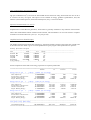
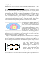
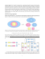
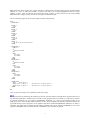
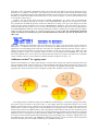
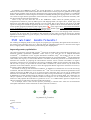
Quild Manual
Quantum-regions Interconnected by Local Descriptions
version 2009.01
Developed by: M. Swart, F. M. Bickelhaupt
Amsterdam, 2004-2009
[email protected]
[email protected]
[email protected]
Contents
What’s new in the 2009.01 version ?
p. 2
GUI-support, Symmetry within QUILD, More QM programs, Frequency calculations, Spin-contamination
correction per region, Improved TS searches, Simplified and more detailed output, Improved primitive
coordinates generation, Frozen coordinates versus constraints, Numerical gradients per region
Basic philosophy
p. 5
Multi-level energy expression
p. 6
AddRemove method for capping atoms
p. 9
Improved geometry optimization
p. 10
Special cases
p. 12
How to call the program
External programs: MOPAC, ORCA, GENERIC
p. 13
Input description
Relevant keywords in QUILD block
CONSTR subblock in QUILD block
FROZEN subblock in QUILD block
SYMROT subblock in QUILD block
TSRC subblock in QUILD block
REGION subblocks in QUILD block
ADDREMOVE subblock in QUILD block
DESCRIPTION subblocks in QUILD block
Numerical versus analytical Hessians for multi-level vibrational frequencies
Use of a GENERIC description for use with user-provided QM-program
Spin-contamination correction per region
INTERACTIONS subblock in QUILD block
INLINE options in the QUILD block
p. 14
p. 14
p. 15
p. 15
p. 15
p. 16
p. 16
p. 16
p. 17
p. 18
p. 18
p. 19
p. 20
p. 20
Example inputfiles
Vibrational frequencies for multi-level QM/QM scheme
Symmetry rotation with Td symmetry for geometry and C2v for orbitals
Optimization with B3LYP through the post-SCF METAGGA scheme
Optimization with B3LYP as SCF functional
Geometry optimization with QM/MM treatment of water dimer
LinearTransit run for bimolecular nucleophilic reaction of F– and CH3Cl
Geometry optimization of pure spin state for spin-contaminated system
LinearTransit run for water dimer
p. 21
p. 21
p. 22
p. 23
p. 23
p. 24
p. 25
p. 26
p. 27
References
p. 28
What’s new in the 2009.01 version
GUI-support
ADFinput has been adapted to provide full support for the multi-level setup in QUILD. See the ADF-GUI pages
for more details.
Symmetry within QUILD
QUILD tries to use symmetry as much as possible, but only for the geometry; as such, more symmetries are
possible than within ADF (for the orbitals). For instance, it enables the use of S4 symmetry for the geometry and
C2 for the orbitals. Moreover, with the use of the SYMROT subblock (see p. 15) one can rotate coordinates from
e.g. D5h to C2v for ferrocene. Therefore, this allows the separation of geometric and orbital symmetry.
More QM programs
Apart from ADF, NewMM and ORCA (for which an interface was already present), the new version includes
interfaces to DFTB and MOPAC, and a GENERIC one to accommodate a generic QM program maintained by the
user itself (see p. 18 for more details). The user-program only has to be able to transform the QUILD-generated
coordinates into an energy/gradient etc. and return data in the format as specified (a simple text file). A working
example for HONDO is available.
Frequency calculations for QM, MM and multi-level QM/QM and QM/MM schemes
Fully operational calculation of the Hessian in case of multi-level schemes, where for each description either an
analytical or numerical setup can be chosen. This can be applied automatically for either QM calculations, MM
calculations, or multi-level QM/MM or QM/QM calculations (including spin-contamination corrections). A full
summary of the important thermodynamic properties (enthalpy at 0K and 298K, entropy, Gibbs free energy) is
reported in the output, for instance:
######################################################################################################
S U M M A R Y
O F
E N E R G Y
T E R M S
######################################################################################################
Pauli Repulsion:
1.234817178116662
33.6011
774.86
3242.01
Electrostatic Interactions:
-0.238553103747176
-6.4914
-149.69
-626.32
Orbital Interactions:
-1.496489120691529
-40.7215
-939.06
-3929.03
Quild Bonding Energy:
-0.500224957131303
-13.6118
-313.90
-1313.34
-----------------------------------------------------------------------------------------------------Zero-Point Energy:
0.020896706726649
0.5686
13.11
54.86
Enthalpy H
(0K):
-0.479328250404654
-13.0432
-300.78
-1258.48
d(Enthalpy H) (0 => 298K):
0.002837412889686
0.0772
1.78
7.45
Enthalpy H
(298K):
-0.476490837514968
-12.9660
-299.00
-1251.03
-T*S
(298K):
-0.021452035100450
-0.5837
-13.46
-56.32
Gibbs-free-energy
(298K):
-0.497942872615418
-13.5497
-312.46
-1307.35
######################################################################################################
2
Spin-contamination correction per region
The spin-contamination (S2) correction has been folded into the multi-level setup, which means the user can do a
S2-correction for only one region. This option is now available for energy, gradients (optimizations, TSs) and
Hessians (vibrational frequencies, numerical and analytical). See p. 19 for more details.
Improved TransitionState (TS) search
Simplification of initial Hessian generation, which makes it generally available for any elements of the Periodic
Table. This should further enhance Transition State searches, which for Baker’s set of 25 TSs results in complete
localization of all TSs within 343 cycles (i.e. 14 cycles per TS).
Simplified and more detailed output
The QUILD output has been drastically reduced (e.g. without the repetitive output of the Create runs in ADF), and
at the same time more detail is given. At each optimization step, the progress of the optimization is reported:
Geometry Optimization Progress
---------------------------------------------------------------------------------------------------Item
Value
Crit
Convgd
---------------------------------------------------------------------------------------------------Gradient Max
0.052637
0.000100
NO
Gradient RMS
0.011095
0.000100
NO
Step Max
0.000000
0.000100
YES
Step RMS
0.000000
0.000100
YES
del(Energy)
-168.585008
0.000010
NO
# neg. Hesseig.
0
0
YES
----------------------------------------------------------------------------------------------------
and the components of the multi-level energy expression are explicitly mentioned:
========================================================================================================
hartree
eV
kcal/mol
kJ/mol
Energy terms for job
1
jobsign: 1 (MOPAC job, SCF energy)
-------------------------------------------------------------------------------------------------------Pauli Repulsion:
0.000000000000
0.0000
0.00
0.00
Electrostatic Interactions:
0.000000000000
0.0000
0.00
0.00
Orbital Interactions:
0.000000000000
0.0000
0.00
0.00
Region Bonding Energy:
-272.352918801950
-7411.1000
-170904.05
-715062.49
Energy terms for job
2
jobsign: 1 (ADF job, SCF energy)
-------------------------------------------------------------------------------------------------------Pauli Repulsion:
65.846536707515
1791.7754
41319.33
172880.06
Electrostatic Interactions:
-5.166530552507
-140.5884
-3242.05
-13564.72
Orbital Interactions:
-66.098012956421
-1798.6184
-41477.13
-173540.31
Region Bonding Energy:
-5.418006801413
-147.4315
-3399.85
-14224.97
Energy terms for job
3
jobsign: -1 (MOPAC job, SCF energy)
-------------------------------------------------------------------------------------------------------Pauli Repulsion:
0.000000000000
0.0000
0.00
0.00
Electrostatic Interactions:
0.000000000000
0.0000
0.00
0.00
Orbital Interactions:
0.000000000000
0.0000
0.00
0.00
Region Bonding Energy:
-109.185918021950
-2971.1000
-68515.21
-286667.59
-------------------------------------------------------------------------------------------------------Total (multi-level) QUILD energy
-------------------------------------------------------------------------------------------------------Quild Bonding Energy:
-168.585007581413
-4587.4315
-105788.70
-442619.87
========================================================================================================
3
Improved generation of primitive coordinates
A new subroutine is used for generating the primitive coordinates, which should lead to less and more important
coordinates (icreate 7).
Frozen coordinates versus constraints
A number of Cartesian coordinates can be kept frozen (with the FROZEN subblock, see p. 15), without the need
to put additional constraints that may be sometimes awkward to put. This can be for instance be the case when the
user wants to treat the active site of an enzyme and freeze certain atoms (e.g. the Cα atoms) to mimic the effect of
the protein environment.
Numerical gradients per region
The numerical gradients that can be used within QUILD are now completely generalized, and can be specified per
region. For instance, if one wants to use the numerical gradient of a hybrid-metagga functional (such as e.g.
mPBE0KCIS) for a small part of the total system, and the analytical gradient of a GGA for the rest, it is simple
and straightforward to achieve this:
QUILD
SMETAGGA mPBE0KCIS
NR_REGIONS=2
INTERACTIONS
TOTAL
description 1
REPLACE region 1
description 3 for description 2
SUBEND
REGION 1
1-3
SUBEND
REGION 2
4-6
SUBEND
DESCRIPTION 1 NEWMM
! MM input for NewMM, not explicitly shown here
SUBEND
DESCRIPTION 2 NEWMM
! MM input for NewMM, not explicitly shown here
SUBEND
DESCRIPTION 3 NUMGRAD MGGA
BASIS
type DZ
core small
END
SCF
Converge 1.0e-7 1.0e-7
Iterations 99
diis ok=0.01
END
INTEGRATION 7.0 7.0 7.0
CHARGE
0.0
METAGGA
SUBEND
END
4
Basic philosophy
The QUILD program1,2 has been developed for enabling calculations through multi-level approaches, in which
different computational treatments are used for different regions of the system under study. The benefit of our
multi-level approach is not only that it can be used to make the calculations cheaper and therefore feasible, but
also that the best method for any type of interaction can be used as we need for DNA (vide infra). For describing
DNA, we use one DFT functional for treating the complete system, and another for π-stacking between the DNA
bases. This is achieved by making the definition of the regions flexible, i.e. there is no need to have a layered
structure as in the ONIOM approach. An arbitrary splitting of the total system into different regions is permitted
with, therefore, possibly overlapping regions; this resembles a quilt, hence the name of the program.
The different treatments currently possible are based on either quantum mechanics (QM) or force field
molecular mechanics (MM). The MM part is provided through the NEWMM program that is included within the
ADF3,4 program package since the 2006.01 version. Density Functional Theory5-7 is provided by the ADF
program, while an interface for the ORCA programi is available for inclusion of Hartree-Fock (RHF/UHF),
Møller-Plesset (MP2) or semi-empirical (e.g. AM1, PM3) calculations. New in the 2009.01 version is the
inclusion of DFTB (for Density Functional Tight Binding), Mopac (semi-empirical, e.g. PM6), and a generic
(QM) program that allows the user to apply his/her own program. In all these cases, the other programs are used
as black-box programs to deliver the energy and gradient, i.e., QUILD writes the inputfiles, runs the black-box
programs, collect the data, makes new coordinates, and repeats this process until the geometry is optimized.
The application of multi-level (QM/QM or QM/MM) approaches within computational chemistry studies is
ever more often used, since it permits to use a highly accurate method for the most important region while treating
the interactions with the surrounding regions at a lower,
yet sufficiently accurate method. The QM/MM setup
(see Figure to the left), where only the region of
interest (region 1, in yellow) is treated with quantum
chemistry methods while the interactions with and
within the surrounding regions is described with
classical molecular mechanics force fields, is the
computationally most economical multi-level approach.
Its accuracy and applicability depend largely on the
accuracy and availability of force field parameters for
the system under study. Specialized force fields are
available for certain classes of chemical systems, such
as the AMBER95 force field8 for proteins and nucleic acids, which is included within the ADF program package
using the NEWMM program. However, the treatment of large biochemical systems containing thousands of atoms
with QUILD is not to be advised due to the making of the adapted delocalized coordinates, involving a
diagonalization step that is not feasible for systems with more than ca. 700 atoms (estimated). Treating large
biochemical systems are best performed by the QM/MM scheme9-11 in ADF.
Because of the computational efficiency, the availability of basis sets for the whole Periodic System, and the
generally accurate results, Density Functional Theory (DFT) has become the method of choice for the majority of
recent computational chemistry studies and can these days almost routinely be used for relatively large system
sizes of up to hundreds of atoms (the largest system used with ADF in single-point calculations contained ca.
1200 atoms; the largest system used within geometry optimizations contained ca. 700 atoms).12-20 However, one
must always remain cautious with the choice of DFT functional and/or basis set, and make sure that the particular
functional is able to give a correct description for the interactions that are important for the system under study.
For instance, the performance of functionals that include the recent OPTX exchange functional21 is superior to
those containing Becke88 exchange,22 for instance
for the accuracy of geometries,23,24 spin state
splittings,25,26 reaction barriers23,27,28 or zero-point
vibrational energies.23 As the improvements can be
3
5
1
5
linked directly to the specific formulation of the
OPTX functional26,29 and its resulting improved
5
5
performance for atomic exchange energies,21 one
would naively think that inclusion of the OPTX
5
2
4
5
functional would always lead to improved
performance. Unfortunately, this is not the case for
weakly bound systems, as shown recently for
i
Note that the ORCA program is not provided within the ADF program package, and the user (or system administrator) has to
download and install the program him/herself. The ORCA program is free of charge for academic groups, more information
can be found at http://www.thch.uni-bonn.de/tc/orca.
5
hydrogen-bonding30 and π-stacking31 in DNA. Moreover, a functional that performs well for hydrogen-bonding
interactions (BP8622,32),30,33-37 does not necessarily give equally good results for π-stacking.31 As a result, at
present there does not seem to be a DFT functional that is equally accurate for hydrogen-bonding, π-stacking and
intramolecular interactions. Therefore, for a study on the structure of DNA duplexes, the multi-level QM/QM
approach2 is needed with one DFT functional for the description of hydrogen-bonding interactions, and another
for the description of π-stacking, which can be exploited within the QUILD scheme.2 In the Figure above, a
schematic structure of DNA is presented with the bases (regions 1 to 4, in orange), and sugars and phosphate
backbone (region 5, in cyan). Since BP86 works well for intramolecular interactions and hydrogen-bonding
interactions, but not for π-stacking, BP86 is used for the whole system, and for the π-stacking its interactions are
replaced by LDA.
Multi-level energy expression
Similar to the ONIOM approach,38,39 the total energy within the multi-level approach is obtained by combining the
different energies, for instance, for the interactions in a protein depicted schematically below, with the active site
(region 1, in yellow), the rest of the protein (region 2, in pink) and solvent (region 3, in blue).
Suppose we want to treat the active site using a GGA functional in a large basis set, the rest of the protein by LDA
in a small basis, and the solvent at MM level. The energy expression is then obtained by a sequence of 5 jobs:
E = E MM (1,2,3) + E LDA (1,2) − E MM (1,2) + E GGA (1) − E LDA (1)
First, the total system is described at the MM level (top-right), then the MM description for regions 1 and 2 is
replaced by LDA (middle-right), and finally the LDA description for region 1 is replaced by the GGA description
(bottom-right).
€ This splitting up of the total system into different jobs is fully automated, the user only has to
assign the different regions and give descriptions for the QM and MM methods to be used.
A second example of using a multi-level approach is posed by the application to DNA. In this case we do not
want to replace all interactions within one region, but merely the interaction between two different regions. This
is again achieved by a sequence of jobs, as indicated in the figure above on the right hand side. First, we have a
6
BP86 job for the whole system (top, in blue). Second, we add the LDA interaction energy for the left-side stacked
basepair in a series of three jobs (middle, in yellow) and remove the corresponding BP86 interaction energy
(middle, in blue). Third, we add the LDA interaction energy (bottom, in pink) and remove the corresponding
BP86 interaction energy (bottom, in blue) for the right-side stacked basepair.
The corresponding input for the second example would be schematically:
QUILD
NR_REGIONS 5
REGION 1
17-30
SUBEND
REGION 2
77-91
SUBEND
REGION 3
47-60
SUBEND
REGION 4
111-122
SUBEND
REGION 5
1-16 31-46 61-76 92-110 123-125
SUBEND
DESCRIPTION 1
CHARGE -2
XC
GGA Becke-Perdew
END
BASIS
type TZ2P
core SMALL
END
SUBEND
DESCRIPTION 2
XC
GGA Becke-Perdew
END
BASIS
type TZ2P
core SMALL
END
SUBEND
DESCRIPTION 3
BASIS
type TZ2P
core SMALL
END
SUBEND
INTERACTIONS
TOTAL
description 1
INTXN region 1 region 2
INTXN region 3 region 4
SUBEND
description 3 for description 2
description 3 for description 2
END
Next, we provide a line-by-line explanation of the above input:
QUILD
All input relevant for performing the QUILD job must be specified within a QUILD block. QUILD takes care of
the remaining input that is needed in runs of ADF or other programs that are invoked (in a "black-box" manner)
by QUILD. Exceptions are, for example, GEOMETRY, GEOVAR, etc., which are specified according to the
ADF input syntax. Thus, detailed input parameters for the various programs that QUILD communicates with can
be passed through to these programs via the QUILD input block (within DESCRIPTION subblocks, see below).
Therefore, any option that is available in ADF (ZORA, COSMO, LDA, GGA, MGGA, HYBRIDS) or in the other
programs (NEWMM, ORCA, DFTB, MOPAC, GENERIC) is also available in QUILD.
7
NR_REGIONS 5
The number of regions is set to five. The definition of the atoms that belong to each region is given in the
REGION subblocks below:
REGION 1
17-30
SUBEND
REGION 2
77-91
SUBEND
REGION 3
47-60
SUBEND
REGION 4
111-122
SUBEND
REGION 5
1-16 31-46 61-76 92-110 123-125
SUBEND
In the above example, atoms 17 to 30 make up region 1 (an equivalent input would be to specify each atom
number individually, i.e.: "17 18 19 20 21 22 23 24 25 26 27 28 29 30"), atoms 77 to 91 region 2, atoms 47 to 60
region 3, atoms 111 to 122 region 4, and the remaining atoms region 5. It is not necessary to define all regions
explicitly: the first job (with the description as defined by the TOTAL line in the INTERACTIONS subblock) includes all
atoms automatically. Only those regions which are explicitly used within the INTERACTIONS subblock need to be
defined, i.e. in this case the definition of region 5 is not actually used. Note that the atom numbers are obtained by
counting consecutively the atoms in the ATOMS block on input.
DESCRIPTION 1
CHARGE -2
XC
GGA Becke-Perdew
END
BASIS
type TZ2P
core SMALL
END
SUBEND
DESCRIPTION 2
XC
GGA Becke-Perdew
END
BASIS
type TZ2P
core SMALL
END
SUBEND
DESCRIPTION 3
BASIS
type TZ2P
core SMALL
END
SUBEND
Given here are the different descriptions that are needed for the BP86 and LDA treatments of the different
regions. Note that there are two different descriptions using BP86, one (DESCRIPTION 1) for the complete system
that has total charge -2, and a second one (DESCRIPTION 2) for the interaction between two stacked bases. For nonADF (i.e. NEWMM, ORCA, DFTB, MOPAC, or GENERIC) jobs, on the first line of the corresponding
DESCRIPTION subblock it should say so, as given in the example below for description 4 (HF/STO-3G with
ORCA):
DESCRIPTION 4 ORCA
! other options for the program are ADF, DFTB, NEWMM, MOPAC, GENERIC
%coords
mult 2
charge -1
end
%method method hf
end
%basis basis sto_3g
end
SUBEND
8
Note that in case of geometry optimizations where one of the jobs uses ORCA, the run-type (keyword runtyp)
should be set to “gradient” in order that a “job*.engrad” file is written (by ORCA) that contains the ORCA energy
and gradient. The QUILD program will automatically add this runtyp keyword to the corresponding input block. If
the ORCA job deals with either an unrestricted job, or with a non-zero charge, it is best to put these data in the
%coords block as shown above.
Together with the general input (apart from ATOMS, GEOMETRY, etc. blocks that are automatically
generated by the QUILD program) the contents of these DESCRIPTION subblocks will constitute the “blackbox” inputfile for the different programs. If there are differences in charge (vide supra), the charges of the total
system and the regions should be given in these DESCRIPTION subblocks. Also when either the region is
Unrestricted and the total system not (or vice versa), the description of being unrestricted (or not) should be given
in the DESCRIPTION subblocks. Note that the general input contents is pasted only into input files for programs
within the ADF program package, for external programs such as ORCA only the automatically generated
atomic coordinates part and the part given in the DESCRIPTION subblock is put into the input file for the
ORCA job.
INTERACTIONS
TOTAL
description 1
INTXN region 1 region 2
INTXN region 3 region 4
SUBEND
description 3 for description 2
description 3 for description 2
This is the subblock that determines how the multi-level job is setup. The total system will be treated by
description 1, i.e. BP86 for all atoms. Then in the second line, the BP86 interaction between regions 1 and 2 is
replaced by the corresponding LDA interaction. In the last line, the BP86 interaction between regions 3 and 4 is
replaced by the LDA interaction. In total there are therefore 5 ADF jobs per geometry cycle. When the ADF
program package is setup to run in parallel, and this is taken care of properly in the $ADFBIN/start script, then
also within QUILD this is used. At present no attempt has been made yet to prepare the interface for the parallel
version of ORCA, the user is responsible for installing the ORCA program (see also p. 13).
AddRemove method40 for capping atoms
Whenever the definition of a region splits through a covalent bond (or better put, whenever QUILD notices that
there are dangling bonds within a certain job), it will automatically add capping atoms to satisfy the valence of the
boundary atoms (see for instance Figure below). For the moment, the program automatically adds hydrogen as
capping atoms, which in the future may be changed to include other elements as well, if needed.
The capping atoms are added according to the AddRemove methodology,40 in which the capping atoms follow
the position of the real atoms in the total system. I.e. the capping atoms are positioned along the vector of the
dangling covalent bond, and at a distance that corresponds to the sum of the covalent radii of the capping atom
and the atom to which the capping atom is attached. Because the capping atoms are added to the active site for
both the high- and low-level QM calculation, with a presumably similar effect in both cases, the interactions of the
capping atoms with the true active site atoms are in good approximation cancelled out (the total effect is removed)
between the lower- and higher-level QM calculations. Within the AddRemove model, the energy and gradients
are treated in similar fashion (unlike other models that project the gradients of the “artificial” capping atoms onto
the gradients of the “real” atoms). The AddRemove model was previously40 shown to perform well for geometries
around the boundary between the QM and MM region in QM/MM calculations.
9
In summary, the AddRemove model40 has several advantages: it is simple, the energy and gradients (and
Hessian) are treated in similar fashion (unlike other models that for instance project the gradients of the capping
atoms onto the gradients of the real atoms). Furthermore, the capping atoms follow the real atoms, at a predefined
distance, and therefore no artificial degrees of freedom are added by including the capping atoms. In a strict sense,
one could even argue that the replacement of the interactions of the capping atoms is performed consistently with
the choices made for the multi-level approach.
There is only one case where the use of the AddRemove model within the QUILD program is not
straightforward, and that is posed by MM regions with dangling bonds (see Figure above, bottom right). The
description of the MM region depends explicitly on a force field, that in turn needs for each atom in the MM
region an atomtype that should be supplied by the user on input, together with all connection tables for all atoms.
As the QUILD program automatically adds capping atoms (H cap in the Figure above), the DESCRIPTION subblock
for the NEWMM description of the capped region (Figure above, bottom right) should include the atomtype and
connections for the automatically added capping (hydrogen) atoms.
The program checks for each job in a multi-level scheme, if they have atoms with dangling bonds. It does this
by going over all regions that are included in that particular job; the order in which the regions are checked
depends on how the regions are given on input (!). For instance, in the following line, region 2 is checked first and
then region 1 as second:
REPLACE
region 2 region 1
description 3 for description 2
For checking the dangling bonds in each region, the program goes sequentially through all atoms and checks if
they belong to that particular region; if so, and if the atom has a dangling bond (as the Cα atom has in the Figure
above) a capping atom is added, which is positioned along this dangling bond.
Improved geometry optimization
One of the strong points of the QUILD program,1,2 apart from its flexible setup of the multi-level approach, is its
enhanced geometry optimization capabilities. These result in part from the use of adapted delocalized
coordinates,41 a modification of the original delocalized coordinates setup42 that enables the use on weak
coordinates as well. Further enhancements are obtained through the use of regulated GDIIS,43,44 Restricted Second
Order model (trust region),45,46 and a model Hessian.41 The latter includes the generation of a model Hessian for
transition state searches by preparing the initial Hessian with the correct curvature and number of negative
eigenvalues, which moreover correspond to the reaction coordinates (TSRC) for the transition state under study.
The user has to specify on input what the relevant TSRC coordinates are, which will not only be used for the
generation of the initial Hessian, but also to select the appropriate Hessian eigenvector when there are more (or
less) than 1 negative Hessian eigenvalues.
The details of setting up the delocalized coordinates, its adaptation to facilitate the use on weak and strong
coordinates, and their characteristics can be found in refs. 41 and 2. Here we briefly mention the performance of the
QUILD program for the Baker test set (a set with 30 organic molecules) and a test set with 18 weakly-bound
molecules.2 For the Baker set, we need 167 iterations to fully converge all molecules to a gradient of 3.0·10-4 a.u.
at RHF/STO-3G (results obtained using the interface to ORCA), and 164 at PW91/TZ2P. For comparison, the
old-style optimizer in ADF using Cartesians needed 222 iterations. For the weakly-bound set, we need 175
iterations to fully optimize the molecules to a gradient of 1.0·10-5 a.u. at PW91/TZ2P. Again for comparison, the
old-style optimizer in ADF using Cartesians needed 748 iterations.
As an example, below is the relevant input for performing a transition state search for the bimolecular
nucleophilic substitution reaction of fluoride on methyl chloride (see figure):
Geometry
TransitionState
End
QUILD
TSRC
dist 1 5
10
dist 1 6
SUBEND
END
ATOMS
C
H
H
H
Cl
F
END
Charge -1
0.000000
-0.530807
-0.530807
1.061614
0.000000
0.000000
0.000000
0.919384693
-0.919384693
0.000000
0.000000
0.000000
0.000000
0.112892
0.112892
0.112892
-2.124300
2.019100
INTEGRATION 6.0 6.0
SCF
converge 1.0e-6 1.0e-6
diis ok=0.01
iterations 99
END
The QUILD program will scan the input for the existence of a Geometry block (that indicates that QUILD should
do an optimization), and will scan the Geometry block for the presence of the TransitionState keyword. If it is
found, it will set the number of negative Hessian eigenvalues that are needed (nrnegneed) to 1, otherwise it will
remain 0.
The QUILD block should in this case contain a TSRC subblock where the coordinates involved in the
transition state are given. In the example above, there are two TSRC coordinates, the C-Cl and the C-F bond, as
indicated by the atom numbers. For the construction of the initial Hessian, a negative force constant is assigned to
these coordinates. For instance in the outputfile, first the definition is given for the primitive coordinates as they
are constructed by the QUILD program (with the TSRC coordinates shown below in blue):
Number of MM coordinates (valence,intramol,intermol) :
32 (
32,
0,
0)
-------------------------------------------------------------------------------valence coordinates
-------------------------------------------------------------------------------1 bnd
2
1
0
0
1
1.02076
2 bnd
3
1
0
0
1
1.02076
3 bnd
4
1
0
0
1
1.02076
4 bnd
5
1
0
0
1
0.50000
5 bnd
6
1
0
0
1
0.50000
6 ang
3
1
2
0
2
0.90892
7 ang
4
1
2
0
2
0.90892
etc.
Further down in the output, the force constants for the different MM coordinates are shown (with the ones for the
TSRC coordinates given in blue):
Force Constants used:
bnd
bnd
etc.
1
5
0.40831
-0.02804
bnd
ang
2
6
0.40831
0.20839
bnd
ang
3
7
0.40831
0.20839
bnd
ang
4
8
-0.03252
0.20839
which are also coupled with each other:
Off-diagonal TSRC Hessian-element :
5
4
-0.04271
-0.02804
-0.03252
And finally, the contributions of the TSRC coordinates to the Hessian eigenvalues is reported:
Weight TSRC-coord
Weight TSRC-coord
1
2
4
5
1.00000 Flindh
1.00000 Flindh
0.50000
0.50000
Contributions of TSRC coordinates to negative Hessian eigenvalue
Contribution from primitive
5
0.49998
Bnd
F
6
Contribution from primitive
4
0.49998
Bnd
CL
5
Contribution from primitive
17
0.00001
Imp
H
3
Contribution from primitive
15
0.00001
Imp
H
4
Contribution from primitive
16
0.00001
Imp
H
4
11
C
C
C
C
C
1 is
1
1
1
1
1
0.99996
H
H
H
4
2
3
H
H
H
2
3
2
Contributions of TSRC coordinates to all Hessian eigenvalues:
Eigval
1 -0.07305
Contrib_All
0.99996
per_tsrc
Eigval
2
0.01248
Contrib_All
0.93816
per_tsrc
0.49998
0.46908
0.49998
0.46908
As a result, the optimization converges within 10 cycles:
QUILD summary for sn2_ts_orig.out
Stp#
Energy
Gmax,adf
Grms,adf
Gmax,deloc.
Grms,deloc.
Symm #negH
(kcal/mol)
(a.u.)
(a.u.)
(a.u.)
(a.u.)
=======================================================================================================
1
-620.9561
0.007101756
0.003028991
0.011855992
0.003715738
C(3V)
1
2
-620.8929
0.023635611
0.007391899
0.013690739
0.005638699
C(3V)
1
3
-621.2068
0.016710875
0.005351311
0.026217447
0.007807519
C(3V)
1
4
-620.8176
0.004699225
0.001709580
0.011879183
0.003484516
C(3V)
1
5
-620.3782
0.008811234
0.002829390
0.018504386
0.005671159
C(3V)
1
6
-620.8564
0.001689444
0.000533251
0.002432001
0.001015262
C(3V)
1
7
-620.9381
0.002213820
0.000584005
0.000987755
0.000448095
C(3V)
1
8
-620.8942
0.000576597
0.000161025
0.000424960
0.000141833
C(3V)
1
9
-620.8840
0.000112994
0.000037557
0.000241219
0.000074629
C(3V)
1
10
-620.8831
0.000010191
0.000003368
0.000021158
0.000006610
C(3V)
1
+++++++++++++++++++++++++++++++++++++++++++++++++++++++++++++++++++++++++++++++++++++++++++++++++
Geometry CONVERGED !!!
Energy at optimized geometry :
-620.8831 (kcal/mol)
+++++++++++++++++++++++++++++++++++++++++++++++++++++++++++++++++++++++++++++++++++++++++++++++++
Additionally, the QUILD optimizer allows to constrain bonds, angles or dihedrals during the optimization, in
which it uses the method by Baker.47 This method has the nice feature that the constraints do not have to be met in
the initial geometry, but are enforced through the use of Lagrangian multipliers. The ability of adding constraints
has been extended to perform a LinearTransit, i.e. a series of constrained optimizations, that can be used to scan a
potential energy surface as function of e.g. a bond. For the SN2 reaction shown above, the relevant input to do a
LinearTransit would be:
QUILD
nrlt 11
CONSTR
dist 1 6 2.5 1.5
SUBEND
END
This means that the C-F distance is reduced (while constrained) in 11 steps, starting from 2.5 Å and going to 1.5
Å, in steps of 0.1 Å. All other coordinates are free to optimize in this example, however a combination of more
than one constrained coordinates is possible; either by including them also as LT coordinate, or simply as
constraint.
Special cases
Because the QUILD program serves as a wrapper around the ADF, NEWMM and ORCA programs, it has
additional capabilities that may not be present within these programs themselves. A numerical evaluation of the
energy gradients in QUILD enables the use of geometry optimization techniques for any methodology within
either of these programs, also for those for which only the energy expression is known or implemented (for
instance meta-GGA or hybrid functionals, Spin-Orbit ZORA, or excited states within ADF) and for which
geometry optimizations are otherwise out of reach (see for example ref. 27 for geometry optimizations with metaGGA functionals, and ref. 2 for optimizations of excited state and spin-orbit geometries). It should be noted that
because of the numerical evaluation of the gradients, requiring 6N+1 energy calculations per geometry step (with
N the number of atoms), these calculations do require a significantly larger CPU-time.
A second additional capability is the possibility to perform a geometry optimization for the pure spin states in
systems that suffer from spin contamination. The spin contamination is simply projected out, not only for the
energy but also for the gradient (and Hessian), by performing two consecutive jobs, one for the contaminated spin
state, a second with the multiplicity increased (that is mixed in into the contaminated job). For instance, the
following example gives an example input:
QUILD
INTERACTIONS
TOTAL description 1
S2CORR description 2
SUBEND
12
DESCRIPTION 1
CHARGE 0.0 1.0
Unrestricted
SUBEND
DESCRIPTION 2
CHARGE 0.0 3.0
Unrestricted
SUBEND
END
See ref. 25 for an example of using this setup on a spin-contaminated system.
How to call the program
The QUILD program is available in the general 2009.01 release of ADF, and should be called in similar fashion
as ADF, e.g.
#! /bin/sh
$ADFBIN/quild << eor
! Normal ADF input, maybe extended with a QUILD inputblock (see below)
eor
The user is responsible for the installation of external programs such as ORCA, MOPAC or a GENERIC program.
For the use of ORCA, the user should make sure that the following works:
orca quildjob.1.inp
and gives the corresponding quildjob.1.engrad file.
For the use with MOPAC the 2009 version of Mopac is needed (see http://openmopac.net), and SCM_MOPAC
should be set to the location where MOPAC is installed. The first line of the MOPAC subblock should contain the
AUX(0) directive, as in the following example:
DESCRIPTION 3 MOPAC
AUX(0) BONDS CHARGE=0 SCFCRT=1.0D-8 PM3 1SCF GRAD
Coordinates generated by ADFinput (c) SCM 1998-2008
SUBEND
Finally, note that the MOPAC subblock should contain 2 lines !
For the use of QUILD with a GENERIC program, the input is straightforward:
DESCRIPTION 3 GENERIC
! Here the specific input for the user-provided GENERIC program
SUBEND
It should be noted that by default, QUILD will use $ADFBIN/quild_generic as script for use with the GENERIC
subblock (this example script facilitates the use of HONDO). However, this can be overridden by setting the
environment variable $QUILD_GENERIC to a user-provided script (see also p. 18).
13
Input description
Relevant keywords in QUILD block
name
CVG_ENR
CVG_GRD
default
1.0e-5
1.0e-4
CVG_STP
DIFSTEP
I_ADD_DUMMIES
1.0e-4
1.0e-5
1
ICREATE
IDCVG
7
1
IDELOCAL
1
IDIIS
3
IDSTEP
5
IEXCST
1
IHOPT
3
IHUPD
-1 cq. 4
IQUILD_OUTPUT
IRESTART
1
0
ITRUST
MXDIIS
MXGEO
0
5
50
NR_REGIONS
NRLT
RTRUST
SMETAGGA
1
0
0.20
-
SYMGEO
TRUST_ALFA
TRUST_BETA
TRUST_GOOD
TRUST_RMIN
1.20
0.70
0.80
0.40
description
Convergence criterium for energy (when IDCVG >= 2)
Convergence criterium for maximum component of gradient; depending on the
value of IDELOCAL, either the delocalized or Cartesian gradient is checked
Convergence criterium for maximum component of step (when IDCVG >= 2)
Stepsize for numerical differentiation (with numerical gradients/Hessian)
Index to do (1) or do not (0) add dummy atoms for avoiding (nearly-)linear
angles
Index which method to use for generating the primitive coordinates
Index how to signal convergence:
1) check nr. of negative Hessian eigenvalues is correct and max. component
and rms value of gradient are less than the convergence criterium (see
CVG_GRD)
3) same as 1, but both max. component of step and change in energy should
be less than their respective convergence criteria (see CVG_STP and
CVG_ENR)
2) same as 3, but only of the additional criteria has to be fulfilled
Kind of coordinates to use in the geometry optimization:
1) adapted delocalized coordinates
0) Cartesian coordinates
Kind of GDIIS equations to use:
0) original GDIIS
1) same as 0, but with Farkas-Schlegel rules applied
2) use gradient as error vector
3) same as 2, but with Farkas-Schlegel rules applied
4) use “energy” vector as error vector
5) same as 4, but with Farkas-Schlegel rules applied
Step to take:
1) RSO for minimizations, RFO (Baker) for TransitionStates
3) RFO (Baker) always
5) Generalized RSO (Swart) using image-function for TransitionStates
Number of excited state to use for numerical gradients
By default for singlet excited state; triplet excited state can be used by
adding ONLYTRIP keyword to EXCITATIONS block on input
Index for force constants method to use for initial Hessian:
0) Baker (0.5 bonds, 0.2 angles, 0.1 dihedrals)
1) Thomas Fischer
2) simplification of Lindh
3) Swart-Bickelhaupt scheme
7) Swart generalized scheme (works well for close to minima)
Index for Hessian update scheme:
1
BFGS for Hessian (-1 BFGS for inverse Hessian)
2
Powell-symmetric-Broyden, PSB (for Transition States)
3
Murtagh-Sargent (Symmetric Rank-One, SR1)
4
Bofill weighted combi of PSB and SR1 (for Transition State)
5
Farkas-Schlegel weighted combi of BFGS and SR1
6
Bakken-Halgaker combi of BFGS and SR1
Amount of output requested, debug output >=2
Index if ADF/ORCA jobs should restart from t21.files from previous geometry
cycles
<0 ORCA uses restart, ADF not
>0 both ORCA and ADF use restart
Index if dynamic trust radius should be used (1) or not (0)
Maximum number of GDIIS vectors to use
Maximum number of geometry cycles (overrides value read from ITERATIONS in
GEOMETRY block)
Number of different regions for multi-level approach
Number of LinearTransit steps
Trust radius value
String for functional from METAGGA post-SCF scheme to use for numerical
gradients, should be given exactly as on METAGGA output
Symmetry to be used within QUILD (default is highest possible)
Factor to increase trust radius if ∆energy agrees with model prediction
Factor to decrease trust radius if ∆energy does not agree with model
Lower threshold for increasing trust radius
Upper threshold for decreasing trust radius
The other keywords that are printed in the output are for debug purposes, under development, or of technical
nature. More information about them can be obtained (if needed) from SCM or M. Swart.
14
CONSTR subblock in QUILD block
Constraints can be supplied in the CONSTR subblock of QUILD. Below are the different option that are possible:
QUILD
CONSTR
dist
angle
dihed
x
y
z
SUBEND
END
1 2
1 2 3
1 2 3 4
1
1
1
0.9
120.0
100.0
0.0
0.0
0.0
! only with idelocal=0
! only with idelocal=0
! only with idelocal=0
The units of these constraints are determined by the parameters in the UNITS block. The numbers in this subblock
refer like usual to the atom numbers, as they are found in the ATOMS block.
A special case is observed for LinearTransit calculations, as given in the example below.
QUILD
nrlt 11
CONSTR
dist
angle
SUBEND
END
1 2
1 2 3
1.0
120.0
2.0
70.0
Here there are two LinearTransit coordinates, i.e. the distance between atoms 1 and 2 and the angle 1-2-3. The
distance between atoms 1 and 4 is a simple constraint throughout the whole calculation.
FROZEN subblock in QUILD block
Another way to introduce constraints is by freezing certain atoms. This can be achieved with the FROZEN
subblock of QUILD, where either all three Cartesian (x, y, z) coordinates of an atom (or a series of atoms) can be
frozen, or only one of the three:
QUILD
FROZEN
x
xyz
SUBEND
END
1-37
48-256
! the X-coordinates of atoms 1 to 37 are kept frozen
! the X,Y,Z-coordinates of atoms 48 to 256 are kept frozen
SYMROT subblock in QUILD block
Sometimes, one wants to lower the symmetry because of more convenient descriptions of d-orbitals of transition
metals for instance. In that case, if one still wants to maintain the higher symmetry for the geometry, one can use
the SYMROT subblock to rotate the coordinates. For instance, for Fe(II)(Cl)42- with Td geometric symmetry, the
Fe d-orbitals are not conveniently separated. This might be better done within C2v symmetry:
Symmetry C(2v)
QUILD
Symgeo T(d)
Symrot
-0.7071067811865475 -0.7071067811865475
-0.7071067811865475 0.7071067811865475
0.0
0.0
Subend
End
Atoms
Fe
Cl
Cl
Cl
Cl
End
0.000000000
-1.326583289
-1.326583289
1.326583289
1.326583289
0.0
0.0
1.0
0.000000000
1.326583289
-1.326583289
1.326583289
-1.326583289
0.000000000
1.326583289
-1.326583289
-1.326583289
1.326583289
15
This transforms the coordinates from Td symmetry:
Atomic coordinates
atom
nr
x (Bohrs)
y (Bohrs)
z (Bohrs)
x (angs)
y (angs)
z (angs)
-------------------------------------------------------------------------------------------FE
1
0.00000
0.00000
0.00000
0.00000
0.00000
0.00000
CL
2
-2.50688
2.50688
2.50688
-1.32658
1.32658
1.32658
CL
3
-2.50688
-2.50688
-2.50688
-1.32658
-1.32658
-1.32658
CL
4
2.50688
2.50688
-2.50688
1.32658
1.32658
-1.32658
CL
5
2.50688
-2.50688
2.50688
1.32658
-1.32658
1.32658
to C2v symmetry:
SYMMETRY C(2V)
Atoms
FE
CL
CL
CL
CL
End
0.000000000
0.000000000
1.876072079
-1.876072079
0.000000000
0.000000000
1.876072079
0.000000000
0.000000000
-1.876072079
0.000000000
1.326583289
-1.326583289
-1.326583289
1.326583289
The particular rotation matrix to be used depends on the choice made by the user for how to represent the
molecule in the lower symmetry (see ADFinput how to impose symmetry).
TSRC subblock in QUILD block
The Transition State Reaction Coordinates that are used to construct the special initial Hessian, should be given in
the TSRC subblock of QUILD. Similar to the CONSTR subblock, the distances, angles, or dihedrals should be specified,
one per line, with atom numbers. The atom numbers should refer to the atoms as they are found in the ATOMS block.
QUILD
TSRC
dist
angle
dihed
SUBEND
END
1 2
1 2 3
1 2 3 4
REGION subblocks in QUILD block
The definition of the different regions should be given in REGION subblocks of QUILD. Although the program counts
the number of regions itself, it should be regarded good practice to make sure that the NR_REGIONS keyword
corresponds to the correct number of REGION subblocks.
QUILD
NR_REGIONS 2
REGION 1
1-11
SUBEND
REGION 2
12 14 13 15 16 17 19 18 22 21 20
SUBEND
END
The order in which the atom numbers are given does not matter, and in order that the input is easier to make and
read, shortcuts are introduced. For instance, the “1-11” shortcut corresponds to “1 2 3 4 5 6 7 8 9 10 11”, etc.
Unlike other multi-level approaches, there is no need to have a shell structure for the different regions. I.e., the
regions can overlap, or be defined as given above for DNA.
ADDREMOVE subblock in QUILD block
There is no ADDREMOVE subblock of QUILD active yet, but in the future it will be added to be able to control how
the capping atoms will be added in the case of regions with dangling bonds. I.e., which elements should be added,
and so on. For the moment, only hydrogens will be added, which works without problems for QM/QM and/or
QM/MM calculations on DNA, or simple peptides. Future developments should decide whether this needs to be
adapted.
16
DESCRIPTION subblocks in QUILD block
In case of multi-level jobs, where different regions are treated with different methodologies, the different
methodologies should be given in the DESCRIPTION subblocks.
QUILD
DESCRIPTION 1 ADF [NUMFREQ]
XC
GGA OPBE
END
BASIS
type TZ2P
core NONE
END
SUBEND
DESCRIPTION 2 ADF NUMGRAD
XC
HYBRID B3LYP
SUBEND
basis
type DZ
core NONE
end
SUBEND
DESCRIPTION 3 ORCA NUMFREQ
%method method hf
runtyp gradient
end
%basis basis sto_3g
end
%coords
mult 2
charge -1
end
SUBEND
DESCRIPTION 4 NEWMM NUMFREQ
QMMM
FORCE_FIELD_FILE $ADFRESOURCES/ForceFields/amber95.ff
QMMM_INFO
-1
OW QM -0.8340 HOH
1 O
2
3
2
HW QM
0.4170 HOH
1 H1
-1
3
HW QM
0.4170 HOH
1 H2
-1
4
OW MM -0.8340 HOH
2 O
5
6
5
HW MM
0.4170 HOH
2 H1
4
6
HW MM
0.4170 HOH
2 H2
4
SUBEND
END
SUBEND
DESCRIPTION 5 DFTB NUMFREQ
CHARGE 0
GEOMETRY
runtype SP
iterations 1
END 1
SUBEND
DESCRIPTION 6 MOPAC NUMFREQ
AUX(0) BONDS CHARGE=0 SCFCRT=1.0D-8 PM3 1SCF GRAD
Coordinates generated by ADFinput (c) SCM 1998-2009
SUBEND
DESCRIPTION 7 GENERIC NUMGRAD NUMFREQ
! input-description specific for GENERIC program for the system under study (see above)
SUBEND
END
Description 1 here applies to OPBE/TZ2P(ae) with ADF, description 2 to B3LYP/DZ(ae) with ADF, description 3
to UHF/STO-3G through the ORCA interface,i and finally descriptions 4 to 7 apply to description for NEWMM,
DFTB, MOPAC and GENERIC respectively.
i
Note that the ORCA program is not provided within the ADF program package, and the user (or system administrator) has to
download and install the program him/herself. The ORCA program is free of charge for academic groups, more information
can be found at http://www.thch.uni-bonn.de/tc/orca.
17
The input for multi-level approaches has been explained above, at p. 7-8. The standard input should be given
for ADF, DFTB and NEWMM. See the corresponding User Manuals for ADF, DFTB and ADF-QM/MM
respectively for them. Also for ORCA should standard input be used, the only exception being the total charge
and multiplicity, which should be given as a partial %coords block. The QUILD program will then add the atomic
coordinates to this block for the “black-box” inputfiles.
Numerical versus analytical Hessians for multi-level vibrational frequencies
The descriptions on the previous page indicate for some of the programs, whether the gradients and Hessians can
be obtained analytically (no extra keywords necessary) or numerically. In the latter case, depending on if it is for
the gradients or Hessian, one should add NUMGRAD or NUMFREQ to the DESCRIPTION line (see previous
page). The QUILD program will then take care of preparing the correct number of jobs etc.
Use of a GENERIC description for use with user-provided QM-program
The 2009.01 version of QUILD allows the user to create his/her own script for use with a QM-program (e.g.
HONDO, Molcas, etc.) for which no standard interface is available yet within QUILD. For this purpose (and with
the GENERIC description above), the QUILD program writes a generalized inputfile for this script that consists
of the following:
Line 1:
NAT IQRUN
NAT
number of atoms
IQRUN type of job:
0 single-point energy
1 single-point energy+grad
2 single-point energy+grad+Hess
Line 2 to NAT+1
ATOM X Y Z
ATOM
atomname
X
Cartesian X-coordinate (in Å)
Y
Cartesian Y-coordinate (in Å)
Z
Cartesian Z-coordinate (in Å)
Remaining lines
User provided lines on input (within DESCRIPTION block)
The user should then make sure that his/her script runs their program, and extract data from it in the following
manner (the QUILD program reads these lines as free format, e.g. spaces or upper/lowercase are not important):
# ---------------------------------------------# lines starting with # will be ignored by QUILD
# ---------------------------------------------# --------------# number of atoms
# --------------[nat]
3
# ---------------------# total energy (Hartree)
# ---------------------[energy]
-74.964263362500
# ---------------------------# cartesian coordinates (Bohr)
# ---------------------------[xyz]
0.0000000
0.0000000
0.0000000
[xyz]
0.0000000
-1.4572640
-1.1166010
[xyz]
0.0000000
1.4572640
-1.1166010
# -------------------# expectation value S2
# -------------------[s2]
0.000000000000
[sz]
0.000000000000
# -----------------------------# energy gradient (Hartree/Bohr)
# -----------------------------[grad]
0.0000000
0.0000000
-0.0424023
[grad]
0.0000000
0.0073465
0.0212011
[grad]
0.0000000
-0.0073465
0.0212011
# -----------------------------# Hessian matrix (Hartree/Bohr2)
# ------------------------------
18
[hess]
[hess]
[hess]
[hess]
[hess]
[hess]
[hess]
[hess]
[hess]
[hess]
[hess]
[hess]
[hess]
[hess]
-0.03797442
0.01898721
0.00000000
0.00000000
0.00000000
-0.01201427
0.00000000
0.00000000
0.00000000
0.01898721
-0.01201427
0.00000000
0.00000000
0.00000000
0.00000000
0.00000000
-0.46505603
0.00000000
0.24554704
0.00000000
-0.46505603
-0.02685307
0.30821802
0.00000000
0.00000000
-0.02685307
0.37088899
-0.30821802
0.00000000
0.00000000
-0.37088899
0.62917145
-0.31458572
0.00000000
-0.24554704
-0.06267097
0.29686554
0.00000000
0.00000000
0.06267097
-0.31458572
0.29686554
0.01898721
0.00000000
0.00000000
0.00000000
0.01898721
-0.00697295
0.00000000
0.00000000
0.00000000
-0.00697295
0.00000000
0.00000000
0.00000000
0.00000000
0.93011207
-0.46505603
-0.24554704
0.00000000
0.00000000
0.49190911
-0.37088899
0.06267097
0.00000000
-0.46505603
0.49190911
-0.06267097
0.00000000
0.00000000
0.37088899
-0.31458572
0.00000000
0.00000000
0.30821802
-0.31458572
0.01772018
0.00000000
0.24554704
-0.30821802
0.01772018
# -----------------------------------------------------# example of data for S2-correction
# in this case the Sz and S2 values should also be given
# -----------------------------------------------------# --------------# number of atoms
# --------------[nat]
2
# ---------------------# total energy (Hartree)
# ---------------------[energy]
-74.362823992381
# ---------------------------# cartesian coordinates (Bohr)
# ---------------------------[xyz]
0.0000000
0.0000000
0.0000000
[xyz]
0.0000000
1.4572640
-1.1166010
# -------------------# expectation value S2
# -------------------[s2]
0.753292786229
[sz]
0.500000000000
Spin-contamination correction per region
Previously, the spin-contamination correction was done for the complete system, but starting from version
2009.01 it can be performed for different regions, as in the following example:
QUILD
DESCRIPTION 1 ADF
Occupations smearq=0.0 &
AA1
4.0
//
AA2
0.0
//
EE1
8.0
//
EE2
6.0
//
AAA1
0.0
//
AAA2
4.0
//
EEE1
6.0
//
EEE2
4.0
//
End
CHARGE 0.0 1.0
Unrestricted
SUBEND
DESCRIPTION 2 ADF
Occupations smearq=0.0 &
AA1
5.0
//
AA2
0.0
//
EE1
8.0
//
EE2
6.0
//
AAA1
0.0
//
AAA2
4.0
//
EEE1
6.0
//
EEE2
4.0
//
End
CHARGE 0.0 3.0
Unrestricted
SUBEND
5.0
0.0
8.0
4.0
0.0
4.0
6.0
4.0
4.0
0.0
8.0
4.0
0.0
4.0
6.0
4.0
19
INTERACTIONS
TOTAL description 1
S2CORR region 1 spin-splus-description 2 for contaminated-description 1
SUBEND
END
SYMMETRY D(5H)
Note that this in this case, the spin-contaminated system (doublet) consists of a triplet-alfa in the EE2-irrep coupled
with a doublet-beta in the AA1-irrep. This is corrected for by a pure quartet, and the corresponding energies
corrected:
Values for S2correction 1 :
s2cont
1.75396
s2pure
0.75000
s2plus
3.78716
a_s2
0.33056
jobsigns job 2
-0.49378
job
1
1.49378
INTERACTIONS subblock in QUILD block
One of the most important input-parts for multi-level jobs is the INTERACTIONS subblock of QUILD, where one should
define how the different descriptions should be applied to the different regions. At the part where we explained
the multi-level approaches, we already showed some examples of how to combine different methodologies. Below
is another example input where all possible options are given.
QUILD
INTERACTIONS
TOTAL
description 1
REPLACE
region 1 region 2
description
REPLACE
region 1
description
INTXN
region 1 region 2
description
S2CORR
region 1 spin-splus-description
SUBEND
END
3
4
3
2
for
for
for
for
description 2
description 3
description 2
contaminated-description 1
If an INTERACTIONS subblock is present (if none is present it means no multi-level setup is done, i.e. pure QM or
MM), there should always be a line with the description of the total system, as shown in the first line of the
INTERACTIONS subblock. Then if you want to replace the interactions for one (or more) region(s), you could do so as
indicated in the second and third line. Finally, if you want to replace the interaction between two regions, as we
need for DNA where we replace the BP86 π-stacking by LDA π-stacking, the fourth line of the INTERACTIONS
subblock should be used. Finally, the last line can be used for spin-contamination corrections for one (or more)
regions.
Note that in all cases it is not necessary at all to add the “region”, “description” and “for” words in the
INTERACTIONS subblock; they are ignored when reading the input. The program reads the line, uses the last two
integers for the descriptions and the ones before for the regions. Therefore, a completely equivalent input would
be as shown below. However, for better readability, it is to be advised to always use the additional text anyway.
QUILD
INTERACTIONS
TOTAL
REPLACE
1 2
REPLACE
1
INTXN
1 2
S2CORR
1
S2CORR
1 3
SUBEND
END
3
4
3
2
2
1
2
3
2
1
1
Note that in the last line, it is indicated that the spin-contamination correction is applied to regions 1 and 3
together.
INLINE options in the QUILD block
Similar to the situation in ADF, one can use the INLINE directive to read specific input-lines from a file rather
than from input. In general, this should make no difference, but in rare instances (for instance if the $ sign is
needed in inputfiles for one of the programs), it might become useful.
20
Example inputfiles
(a set with many more examples is provided in the $ADFHOME/examples/quild directory)
Vibrational frequencies for multi-level QM/QM scheme
$ADFBIN/quild << eor
ATOMS
C
-0.759255999
C
0.759255999
H
-1.179949313
H
-1.179949313
H
-1.115011042
H
1.179949313
H
1.179949313
H
1.115011042
END
0.032048841
-0.032048841
-0.464915468
-0.464915468
1.076188400
0.464915468
0.464915468
-1.076188400
0.000000000
0.000000000
0.890460461
-0.890460461
0.000000000
0.890460461
-0.890460461
0.000000000
GEOMETRY
Frequencies
END
AnalyticalFreq
End
Integration 7.0 7.0
SCF
converge 1.0e-7 1.0e-7
diis ok=0.01
END
QUILD
NR_REGIONS=2
REGION 1
1-8
SUBEND
REGION 2
2 6-8
SUBEND
DESCRIPTION 1 ADF
BASIS
type DZ
core Large
END
SUBEND
DESCRIPTION 2 ADF
! adding NUMFREQ would use numerical Hessian (not necessary in this case,
! because Analytical Hessian is available)
BASIS
type TZP
core Large
END
SUBEND
INTERACTIONS
TOTAL description 1
REPLACE region 2 description 2 for description 1
SUBEND
END
END INPUT
eor
rm quildjob*
21
Symmetry rotation with Td symmetry for geometry and C2v for orbitals
$ADFBIN/quild << eor
Title JCTC systems
Occupations smearq=0.0 &
A1
10.0
A2
3.0
B1
6.0
B2
6.0
End
//
//
//
//
9.0
2.0
5.0
5.0
Symmetry C(2v)
QUILD
Symgeo T(d)
Symrot
-0.7071067811865475 -0.7071067811865475 0.0
-0.7071067811865475 0.7071067811865475 0.0
0.0 0.0 1.0
Subend
End
Atoms
Fe
Cl
Cl
Cl
Cl
End
0.000000000
-1.326583289
-1.326583289
1.326583289
1.326583289
0.000000000
1.326583289
-1.326583289
1.326583289
-1.326583289
0.000000000
1.326583289
-1.326583289
-1.326583289
1.326583289
Geometry
End
Charge -2 4
Unrestricted
XC
LDA VWN
GGA OPBE
END
BASIS
type TZ2P
core SMALL
END
SCF
converge 1.0e-6 1.0e-6
iterations 99
diis ok=0.01
END
INTEGRATION 6.0 6.0
EPRINT
SFO noeig noovl
END
endinput
eor
22
Optimization with B3LYP through the post-SCF METAGGA scheme
$ADFBIN/quild << eor
title Geometry optimization
EPRINT
SFO NOEIG NOOVL
END
XC
GGA BLYP
END
ATOMS
O
.000000
.000000
C
.000000
.000000
END
BASIS
type DZ
core NONE
END
GEOMETRY
END
SCF
diis ok=0.01
converge 1.0e-5 1.0e-5
END
QUILD
cvg_grd 1.0e-4
numgrad 1
SMETAGGA B3LYP(VWN5)
END
METAGGA
HFEXCHANGE
INTEGRATION 5.0 5.0
endinput
eor
.000000
1.128100
Optimization with B3LYP as SCF functional
$ADFBIN/quild << eor
title Geometry optimization
EPRINT
SFO NOEIG NOOVL
END
XC
HYBRID B3LYP
END
ATOMS
O
.000000
.000000
C
.000000
.000000
END
BASIS
type DZ
core NONE
END
GEOMETRY
END
SCF
diis ok=0.01
converge 1.0e-5 1.0e-5
END
QUILD
cvg_grd 1.0e-4
numgrad 2
END
INTEGRATION 5.0 5.0
endinput
eor
.000000
1.128100
23
Geometry optimization with QM/MM treatment of water dimer
$ADFBIN/quild << eor
TITLE QM/MM calculation setup by pdb2adf: M.Swart, 2005
GEOMETRY
END
ATOMS
O
0.0000
H
-0.5220
H
-0.5220
O
0.0000
H
0.0570
H
0.9110
END
0.0000
0.2660
0.2660
-3.2000
-2.2440
-3.4950
0.0000
-0.7570
0.7570
0.0000
0.0000
0.0000
QUILD
NR_REGIONS=2
INTERACTIONS
TOTAL
description 1
REPLACE region 1
description 3 for description 2
SUBEND
REGION 1
1-3
SUBEND
REGION 2
4-6
SUBEND
DESCRIPTION 1 NEWMM
QMMM
FORCE_FIELD_FILE $ADFRESOURCES/ForceFields/amber95.ff
MM_CONNECTION_TABLE
1 OW QM
2
3
2 HW QM
1
3 HW QM
1
4 OW MM
5
6
5 HW MM
4
6 HW MM
4
SUBEND
CHARGES
1 -0.8340
2
0.4170
3
0.4170
4 -0.8340
5
0.4170
6
0.4170
SUBEND
END
SUBEND
DESCRIPTION 2 NEWMM
QMMM
FORCE_FIELD_FILE $ADFRESOURCES/ForceFields/amber95.ff
MM_CONNECTION_TABLE
1 OW QM
2
3
2 HW QM
1
3 HW QM
1
SUBEND
CHARGES
1 -0.8340
2
0.4170
3
0.4170
SUBEND
END
SUBEND
DESCRIPTION 3
EPRINT
SFO NOEIG NOOVL
END
XC
24
GGA Becke-Perdew
END
BASIS
type TZP
core small
END
SCF
Converge 1.0e-5 1.0e-5
Iterations 99
END
INTEGRATION 5.0 5.0 5.0
CHARGE
0.0
SUBEND
END
ENDINPUT
eor
LinearTransit run for bimolecular nucleophilic reaction of F– and CH3Cl
$ADFBIN/quild << eor
Title LinearTransit for Sn2 reaction of F- + CH3Cl
XC
GGA OPBE
END
QUILD
nrlt 11
cvg_grd 1.0e-4
CONSTR
dist 1 6 2.5 1.5
SUBEND
END
ATOMS
C
H
H
H
Cl
F
END
0.000000
-0.530807
-0.530807
1.061614
0.000000
0.000000
0.000000
0.000000
0.919384693
0.112892
-0.919384693
0.112892
0.000000
0.112892
0.000000
-1.724300
0.000000
2.500000
Geometry
End
BASIS
type TZ2P
core NONE
END
INTEGRATION 6.0 6.0
SCF
converge 1.0e-6 1.0e-6
diis ok=0.01
iterations 99
END
Charge -1
EPRINT
SFO noeig noovl
END
endinput
eor
25
Geometry optimization of pure spin state for spin-contaminated system
$ADFBIN/quild << eor
Title InorgChimActa paper
EPRINT
SFO NOEIG NOOVL
END
XC
GGA OPBE
END
GEOMETRY
END
BASIS
type TZP
core SMALL
END
SCF
Iterations 99
Diis ok=0.01
Mix 0.1
converge 1.0e-6 1.0e-6
END
INTEGRATION 6.0 6.0 6.0
QUILD
INTERACTIONS
TOTAL description 1
S2CORR description 2
SUBEND
DESCRIPTION 1
Occupations smearq=0.0 &
AA1
4.0
//
AA2
0.0
//
EE1
8.0
//
EE2
6.0
//
AAA1
0.0
//
AAA2
4.0
//
EEE1
6.0
//
EEE2
4.0
//
End
CHARGE 0.0 1.0
Unrestricted
SUBEND
DESCRIPTION 2
Occupations smearq=0.0 &
AA1
5.0
//
AA2
0.0
//
EE1
8.0
//
EE2
6.0
//
AAA1
0.0
//
AAA2
4.0
//
EEE1
6.0
//
EEE2
4.0
//
End
CHARGE 0.0 3.0
Unrestricted
SUBEND
5.0
0.0
8.0
4.0
0.0
4.0
6.0
4.0
4.0
0.0
8.0
4.0
0.0
4.0
6.0
4.0
END
SYMMETRY D(5H)
ATOMS
V
C
C
C
0.00000
1.20500
0.37237
-0.97487
0.00000
-1.66000
-1.66000
-1.66000
0.00000
0.00000
1.14602
0.70828
26
C
C
H
H
H
H
H
C
C
C
C
C
H
H
H
H
H
END
-0.97487
0.37237
2.29965
0.71063
-1.86046
-1.86046
0.71063
-0.97487
0.37237
1.20500
0.37237
-0.97487
-1.86046
0.71063
2.29965
0.71063
-1.86046
-1.66000
-1.66000
-1.70014
-1.70014
-1.70014
-1.70014
-1.70014
1.66000
1.66000
1.66000
1.66000
1.66000
1.70014
1.70014
1.70014
1.70014
1.70014
-0.70828
-1.14602
0.00000
2.18710
1.35170
-1.35170
-2.18710
0.70828
1.14602
0.00000
-1.14602
-0.70828
1.35170
2.18710
0.00000
-2.18710
-1.35170
endinput
eor
LinearTransit run for water dimer
$ADFBIN/quild << eor
TITLE QUILD (QUantum-regions Interconnected by Local Descriptions) input
QUILD
Constr
dist 1 2 2.6 3.4
Subend
nrlt 9
cvg_grd 1.0e-4
END
XC
GGA PW91
END
BASIS
TYPE DZP
CORE small
END
INTEGRATION 6.0 6.0
SCF
converge 1.0e-6 1.0e-6
diis ok=0.01 n=5 bfac=0.2
iterations 99
END
GEOMETRY
END
Occupations smearq=0.0
ATOMS
O
O
H
H
H
H
END
-1.262468
1.537530
-1.540482
-1.540482
0.654929
2.150974
-0.389110
0.425178
0.138323
0.138323
0.010487
-0.323200
0.000000
0.000000
0.765971
-0.765971
0.000000
0.000000
EPRINT
SFO NOEIG NOOVL
END
ENDINPUT
eor
27
References
1.
2.
3.
4.
5.
6.
7.
8.
9.
10.
11.
12.
13.
14.
15.
16.
17.
18.
19.
20.
21.
22.
23.
24.
25.
26.
27.
28.
29.
30.
31.
32.
33.
34.
35.
36.
37.
38.
39.
40.
41.
42.
43.
44.
45.
46.
47.
Swart, M.; Bickelhaupt, F. M. Amsterdam, 2006.
Swart, M.; Bickelhaupt, F. M. J Comput Chem 2007, submitted.
Baerends, E. J.; Autschbach, J.; Bérces, A.; Bickelhaupt, F. M.; Bo, C.; de Boeij, P. L.; Boerrigter, P. M.; Cavallo, L.; Chong, D.
P.; Deng, L.; Dickson, R. M.; Ellis, D. E.; Fan, L.; Fischer, T. H.; Fonseca Guerra, C.; van Gisbergen, S. J. A.; Groeneveld, J. A.;
Gritsenko, O. V.; Grüning, M.; Harris, F. E.; van den Hoek, P.; Jacob, C. R.; Jacobsen, H.; Jensen, L.; van Kessel, G.; Kootstra, F.;
van Lenthe, E.; McCormack, D. A.; Michalak, A.; Neugebauer, J.; Osinga, V. P.; Patchkovskii, S.; Philipsen, P. H. T.; Post, D.;
Pye, C. C.; Ravenek, W.; Ros, P.; Schipper, P. R. T.; Schreckenbach, G.; Snijders, J. G.; Solà, M.; Swart, M.; Swerhone, D.; te
Velde, G.; Vernooijs, P.; Versluis, L.; Visscher, L.; Visser, O.; Wang, F.; Wesolowski, T. A.; van Wezenbeek, E.; Wiesenekker, G.;
Wolff, S. K.; Woo, T. K.; Yakovlev, A. L.; Ziegler, T.; SCM: Amsterdam, 2006.
te Velde, G.; Bickelhaupt, F. M.; Baerends, E. J.; Fonseca Guerra, C.; van Gisbergen, S. J. A.; Snijders, J. G.; Ziegler, T. J Comput
Chem 2001, 22, 931.
Koch, W.; Holthausen, M. C. A Chemist's Guide to Density Functional Theory; Wiley-VCH: Weinheim, 2000.
Parr, R. G.; Yang, W. Density functional theory of atoms and molecules; Oxford University Press: New York, 1989.
Dreizler, R.; Gross, E. Density Functional Theory; Plenum Press: New York, 1995.
Cornell, W. D.; Cieplak, P.; Bayly, C. I.; Gould, I. R.; Merz Jr., K. M.; Ferguson, D. M.; Spellmeyer, D. C.; Fox, T.; Caldwell, J.
W.; Kollman, P. A. J Am Chem Soc 1995, 117, 5179.
Woo, T. K.; Blöchl, P. E.; Ziegler, T. J Mol Struct (THEOCHEM) 2000, 506, 313.
Woo, T. K.; Cavallo, L.; Ziegler, T. Theor Chem Acc 1998, 100, 307.
Woo, T. K.; Margl, P. M.; Deng, L.; Cavallo, L.; Ziegler, T. Catal Today 1999, 50, 479.
Kamachi, T.; Yoshizawa, K. J Am Chem Soc 2003, 125, 4652.
Perdew, J. P.; Ruzsinszky, A.; Tao, J. M.; Staroverov, V. N.; Scuseria, G. E.; Csonka, G. I. J Chem Phys 2005, 123, 062201.
Rosa, A.; Ricciardi, G.; Baerends, E. J. J Phys Chem A 2006, 110, 5180.
Schoneboom, J. C.; Lin, H.; Reuter, N.; Thiel, W.; Cohen, S.; Ogliaro, F.; Shaik, S. J Am Chem Soc 2002, 124, 8142.
Costas, M.; Ribas, X.; Poater, A.; López Valbuena, J. M.; Xifra, R.; Company, A.; Duran, M.; Solà, M.; Llobet, A.; Corbella, M.;
Usón, M. A.; Mahía, J.; Solans, X.; Shan, X. P.; Benet-Buchholz, J. Inorg Chem 2006, 45, 3569.
Sala, X.; Plantalech, E.; Romero, I.; Rodríguez, M.; Llobet, A.; Poater, A.; Duran, M.; Solà, M.; Jansat, S.; Gómez, M.; Parella, T.;
Stoeckli-Evans, H.; Benet-Buchholz, J. Chem-Eur J 2006, 12, 2798.
Poater, A.; Moradell, S.; Pinilla, E.; Poater, J.; Solà, M.; Martínez, M. A.; Llobet, A. Dalton Transactions 2006, 1188.
Martín, N.; Altable, M.; Filippone, S.; Martín-Domenech, A.; Poater, A.; Solà, M. Chem-Eur J 2005, 11, 2716.
Duran, J.; Polo, A.; Real, J.; Benet-Buchholz, J.; Poater, A.; Solà, M. Eur J Inorg Chem 2003, 4147.
Handy, N. C.; Cohen, A. J. Molec Phys 2001, 99, 403.
Becke, A. D. Phys Rev A 1988, 38, 3098.
Swart, M.; Ehlers, A. W.; Lammertsma, K. Molec Phys 2004, 102, 2467.
Swart, M.; Snijders, J. G. Theor Chem Acc 2003, 110, 34.
Swart, M. Inorg Chim Acta 2007, 360, 179.
Swart, M.; Groenhof, A. R.; Ehlers, A. W.; Lammertsma, K. J Phys Chem A 2004, 108, 5479.
Swart, M.; Solà, M.; Bickelhaupt, F. M. J Comput Chem 2007, in press.
de Jong, G. Th.; Bickelhaupt, F. M. J Chem Theor Comp 2006, 2, 322.
Grüning, M.; Gritsenko, O.; Baerends, E. J. J Phys Chem A 2004, 108, 4459.
van der Wijst, T.; Fonseca Guerra, C.; Swart, M.; Bickelhaupt, F. M. Chem Phys Lett 2006, 426, 415.
Swart, M.; van der Wijst, T.; Fonseca Guerra, C.; Bickelhaupt, F. M. J Comput Chem 2007, to be submitted.
Perdew, J. P. Phys Rev B 1986, 33, 8822.
Fonseca Guerra, C.; Bickelhaupt, F. M. Angew Chem Int Ed 1999, 38, 2942.
Fonseca Guerra, C.; Bickelhaupt, F. M. Angew Chem Int Ed 2002, 41, 2092.
Fonseca Guerra, C.; Bickelhaupt, F. M.; Baerends, E. J. Cryst Growth Des 2002, 2, 239.
Fonseca Guerra, C.; Bickelhaupt, F. M.; Snijders, J. G.; Baerends, E. J. Chem-Eur J 1999, 5, 3581.
Fonseca Guerra, C.; Bickelhaupt, F. M.; Snijders, J. G.; Baerends, E. J. J Am Chem Soc 2000, 122, 4117.
Vreven, T.; Morokuma, K. J Chem Phys 2000, 113, 2969.
Svensson, M.; Humbel, S.; Froese, R. D. J.; Matsubara, T.; Sieber, S.; Morokuma, K. J Phys Chem 1996, 100, 19357.
Swart, M. Int J Quant Chem 2003, 91, 177.
Swart, M.; Bickelhaupt, F. M. Int J Quant Chem 2006, 106, 2536.
Baker, J.; Kessi, A.; Delley, B. J Chem Phys 1996, 105, 192.
Csaszar, P.; Pulay, P. J Molec Struct 1984, 114, 31.
Farkas, O.; Schlegel, H. B. Phys Chem Chem Phys 2002, 4, 11.
Yeager, D. L.; Jensen, H. J. A.; Jørgensen, P.; Helgaker, T. U. In Geometrical derivatives of energy surfaces and molecular
properties; Jørgensen, P.; Simons, J., Eds.; Reidel Publishing: Dordrecht, 1986, p 229.
Bakken, V.; Helgaker, T. J Chem Phys 2002, 117, 9160.
Baker, J. J Comput Chem 1997, 18, 1079.
28