Download Implementing a Time Optimal Task Sequence For Robot

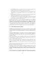
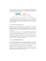
UPTEC IT 14 011
Examensarbete 30 hp
Juni 2014
Implementing a Time Optimal
Task Sequence For Robot Assembly
Using Constraint Programming
Joakim Ejenstam
Abstract
Implementing a Time Optimal Task Sequence For
Robot Assembly Using Constraint
Joakim Ejenstam
Teknisk- naturvetenskaplig fakultet
UTH-enheten
Besöksadress:
Ångströmlaboratoriet
Lägerhyddsvägen 1
Hus 4, Plan 0
Postadress:
Box 536
751 21 Uppsala
Telefon:
018 – 471 30 03
Telefax:
018 – 471 30 00
Hemsida:
http://www.teknat.uu.se/student
Assembly lines in a lean production environment may persist for months or years, but
due to the rapid change in demands on the consumer market they can be subject to
quick changes. Robots have been proved to handle tasks that previously were limited
to human workers: this is the goal of the flexible two armed robot developed by ABB.
When installing a new robot into an assembly line there are several parameters which
make it a difficult job for programmers, even experienced ones, to install the robot.
These problems lead to long installation processes that can take weeks, and there are
great benefits of automating the process of finding good solutions to the problem. In
this thesis a constraint programming approach is presented as a way to solve the
complex sequencing problem when installing a two armed robot into a new
environment. When benchmarked against a reference case study, the implemented
prototype solutions showed an improvement of 17%, all within a time limit of 20
minutes instead of weeks. This shows that constraint programming can be a good tool
for automating robot installations.
Handledare: Johan Wessén
Ämnesgranskare: Pierre Flener
Examinator: Lars-Åke Nordén
ISSN: 1401-5749, UPTEC IT 14 011
Tryckt av: Reprocentralen ITC
Popular Scientific Summary in Swedish
I ett steg att möta snabbt föränderliga produktionsmiljöer som är vanligt förekommande
inom konsumentelektroniktillverkning där arbetsuppgiften för arbetarna kan ändras
inom loppet av några månader har ABB tagit fram konceptroboten FRIDA. FRIDAroboten är en tvåarmad robot i samma storlek som en vuxen människa och har som
mål att vara lätt att installera i ett arbetsutrymme som är gjort för en människa. Ett
problem vid installationen av FRIDA-roboten som har visat sig är den komplexitet i att
översätta en människas arbete till instruktioner för roboten på ett effektivt sätt. Installationstider har visat sig kunna ta flera veckor vilket inte är hållbart i sammanhanget av
en produktionsmiljö som kan ändras inom loppet av några månader.
Målet med arbetet har varit att undersöka och demonstrera möjligheten att automatisera
installationsprocessen av en FRIDA-robot med hjälp av villkorsprogrammering. Villkorsprogrammering är en programmeringsparadigm för att lösa kombinatoriska problem genom att modellera problem med variabler och deras relationer. Fördelen med att
använda villkorsprogrammering för att automatisera installationen av FRIDA-roboten
är den relativa enkelheten i att uttrycka krav och begränsningar i problemet i modellen.
För att demonstrera användandet av villkorsprogrammering vid automatiserade installationer har en referensinstallation används. Utifrån denna installation och med ett
Vehicle Routing Problem (VRP) som utgångspunkt har en modell skapats och en sökstrategi tagits fram för att kunna hitta bra sekvenser.
Experiment med ett antal parametrar som för att kunna styra lösningsprocessen har
genomförts. Detta för att kunna hitta en uppsättning med parametrar som effektivt kan
hitta möjliga sekvenser för roboten i en 20 minuters tidsram. För att kunna jämföra de
resultaten som villkorslösaren gav och den lösningen som tillämpades i referensinstallationen simulerades körtider för roboten i programvaran Robot Studio. Referensinstallationens tid tillhandahölls genom att lösa problemet med den givna sekvensen och
på så sätt erhålla en körtid som kunde jämföras med modellens lösningar.
Utifrån de resultat som experimenten visade på kan slutsatsen dras att villkorsprogrammering är ett lämpligt verktyg för att automatiskt hitta bra lösningar på problemet med
att installera FRIDA-roboten. Samtliga lösningar som villkorslösaren hittade visade på
en bättre körtid än referensen och fanns inom en 20 minuters tidsgräns vilket är ett godkänt resultat. Samtidigt öppnar resultaten upp för vidare undersökning av problemet
för att förbättra lösningarna.
4
Acknowledgements
The work with this thesis project has been educational and interesting. I’ve gotten
insight into how a large industrial company like ABB operates and the interesting world
of robotics.
I would like to thank my supervisor Johan Wessén at ABB Corporate Research for all
the help and support and for many a good discussion about the problem and optimisation technologies.
I would also like to thank my reviewer Pierre Flener for his invaluable feedback during
the writing of the thesis.
A special thank you goes out to Ivan Lundberg, Mikael Hedelind and Peter Fransson
at ABB for their time to answer any question about the FRIDA project and help to
provide simulated data to perform the evaluations and benchmarks.
Last I would like to thank all the persons at ABB who, during my time at the office, all
made it a good working environment.
3
Contents
1
Introduction
1.1 Setting . . . . . . . . . .
1.2 Project Purpose and Goal
1.3 Scope . . . . . . . . . .
1.4 Structure of the Report .
.
.
.
.
.
.
.
.
.
.
.
.
.
.
.
.
.
.
.
.
.
.
.
.
.
.
.
.
.
.
.
.
.
.
.
.
.
.
.
.
.
.
.
.
.
.
.
.
.
.
.
.
.
.
.
.
.
.
.
.
.
.
.
.
.
.
.
.
7
7
7
8
8
2
Background
2.1 ABB Robotics and the FRIDA Robot . .
2.2 Assembly Graphs . . . . . . . . . . . .
2.3 The Lean Production Environment Cell
2.4 Optimising the Task Sequence . . . . .
.
.
.
.
.
.
.
.
.
.
.
.
.
.
.
.
.
.
.
.
.
.
.
.
.
.
.
.
.
.
.
.
.
.
.
.
.
.
.
.
.
.
.
.
.
.
.
.
.
.
.
.
.
.
.
.
.
.
.
.
.
.
.
.
10
10
10
11
12
3
The Vehicle Routing Problem
3.1 The Travelling Salesperson Problem . . . . . . . . . . . . . . .
3.2 Generalising the TSP . . . . . . . . . . . . . . . . . . . . . . .
3.3 Defining the Vehicle Routing Problem . . . . . . . . . . . . . .
3.4 Variations of the VRP . . . . . . . . . . . . . . . . . . . . . . .
3.4.1 Capacitated Vehicle Routing Problem . . . . . . . . . .
3.4.2 Vehicle Routing Problem with Time Windows . . . . . .
3.4.3 Pick-up and Delivery Problem . . . . . . . . . . . . . .
3.5 Common Approaches to Solve the VRP . . . . . . . . . . . . .
3.5.1 Genetic Programming . . . . . . . . . . . . . . . . . .
3.5.2 Ant Colony Optimisation . . . . . . . . . . . . . . . . .
3.5.3 Local Search . . . . . . . . . . . . . . . . . . . . . . .
3.5.4 Constraint Programming . . . . . . . . . . . . . . . . .
3.5.5 Large Neighbourhood Search and Other Hybrid Methods
3.6 The Job Shop Problem . . . . . . . . . . . . . . . . . . . . . .
3.7 The VRP of the Thesis Project . . . . . . . . . . . . . . . . . .
.
.
.
.
.
.
.
.
.
.
.
.
.
.
.
.
.
.
.
.
.
.
.
.
.
.
.
.
.
.
.
.
.
.
.
.
.
.
.
.
.
.
.
.
.
14
14
14
14
15
15
15
16
16
16
16
17
18
18
19
20
4
Constraint Programming
4.1 Constraint Satisfaction Problems . . . . . . . . . . . .
4.2 Constrained Optimisation Problems . . . . . . . . . .
4.3 Propagation . . . . . . . . . . . . . . . . . . . . . . .
4.4 Consistency . . . . . . . . . . . . . . . . . . . . . . .
4.5 Search . . . . . . . . . . . . . . . . . . . . . . . . . .
4.5.1 Branching . . . . . . . . . . . . . . . . . . . .
4.5.2 Heuristics . . . . . . . . . . . . . . . . . . . .
4.5.3 Exploration . . . . . . . . . . . . . . . . . . .
4.6 Reification . . . . . . . . . . . . . . . . . . . . . . . .
4.7 Global Constraints . . . . . . . . . . . . . . . . . . .
4.7.1 The AllDifferent Constraint (A LL D IFFERENT)
4.7.2 The Element Constraint (E LEMENT) . . . . . .
4.7.3 The Count Constraint (C OUNT) . . . . . . . .
4.7.4 The Transition Constraint (I N _R ELATION) . .
4.7.5 The Disjunctive Constraint (D ISJUNCTIVE) . .
4.7.6 The NoCycle Constraint (C IRCUIT) . . . . . .
4.8 Large Neighbourhood Search . . . . . . . . . . . . . .
4.9 Interval Decision Variables . . . . . . . . . . . . . . .
.
.
.
.
.
.
.
.
.
.
.
.
.
.
.
.
.
.
.
.
.
.
.
.
.
.
.
.
.
.
.
.
.
.
.
.
.
.
.
.
.
.
.
.
.
.
.
.
.
.
.
.
.
.
22
22
22
23
23
24
24
25
25
27
27
27
28
28
28
28
29
29
30
.
.
.
.
.
.
.
.
.
.
.
.
.
.
.
.
.
.
.
.
5
.
.
.
.
.
.
.
.
.
.
.
.
.
.
.
.
.
.
.
.
.
.
.
.
.
.
.
.
.
.
.
.
.
.
.
.
.
.
.
.
.
.
.
.
.
.
.
.
.
.
.
.
.
.
.
.
.
.
.
.
.
.
.
.
.
.
.
.
.
.
.
.
.
.
.
.
.
.
.
.
.
.
.
.
.
.
.
.
.
.
.
.
.
.
.
.
.
.
4.10 Google OR-Tools . . . . . . . . . . . . . . . . . . . . . . . . . . . .
30
5
Implementation of the Constraint Model
5.1 The FRIDA Cell Case Study . . . . . . . .
5.2 Model . . . . . . . . . . . . . . . . . . . .
5.2.1 Core Constraints . . . . . . . . . .
5.2.2 Objective Function . . . . . . . . .
5.3 FRIDA Robot Sequencing Side Constraints
5.3.1 Precedences . . . . . . . . . . . . .
5.3.2 Avoiding Arm Collisions . . . . . .
5.3.3 Capacity . . . . . . . . . . . . . .
5.3.4 Route Allocation . . . . . . . . . .
5.4 Search Strategy and Branching Heuristics .
5.4.1 Systematic Tree Search . . . . . . .
5.4.2 Local Search . . . . . . . . . . . .
.
.
.
.
.
.
.
.
.
.
.
.
.
.
.
.
.
.
.
.
.
.
.
.
.
.
.
.
.
.
.
.
.
.
.
.
.
.
.
.
.
.
.
.
.
.
.
.
.
.
.
.
.
.
.
.
.
.
.
.
.
.
.
.
.
.
.
.
.
.
.
.
.
.
.
.
.
.
.
.
.
.
.
.
.
.
.
.
.
.
.
.
.
.
.
.
.
.
.
.
.
.
.
.
.
.
.
.
.
.
.
.
.
.
.
.
.
.
.
.
.
.
.
.
.
.
.
.
.
.
.
.
.
.
.
.
.
.
.
.
.
.
.
.
.
.
.
.
.
.
.
.
.
.
.
.
.
.
.
.
.
.
.
.
.
.
.
.
31
31
31
34
36
36
37
38
39
40
42
42
42
6
Results
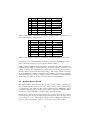
6.1 Experiment Setup . . . . . . . . . . . . . .
6.2 Model Settings . . . . . . . . . . . . . . .
6.3 Systematic Tree Search . . . . . . . . . . .
6.4 Random Restart Search . . . . . . . . . . .
6.5 Objective Function Variation . . . . . . . .
6.6 Local Search . . . . . . . . . . . . . . . .
6.7 Impact of Using Different Tools for Pick-up
6.8 Compared to the Reference Solution . . . .
.
.
.
.
.
.
.
.
.
.
.
.
.
.
.
.
.
.
.
.
.
.
.
.
.
.
.
.
.
.
.
.
.
.
.
.
.
.
.
.
.
.
.
.
.
.
.
.
.
.
.
.
.
.
.
.
.
.
.
.
.
.
.
.
.
.
.
.
.
.
.
.
.
.
.
.
.
.
.
.
.
.
.
.
.
.
.
.
.
.
.
.
.
.
.
.
.
.
.
.
.
.
.
.
.
.
.
.
.
.
.
.
44
44
45
45
46
47
47
48
49
7
Conclusions
7.1 Systematic Tree Search
7.2 Randomised Restart . .
7.3 Local Search . . . . .
7.4 Objective Functions . .
7.5 Conclusion . . . . . .
.
.
.
.
.
.
.
.
.
.
.
.
.
.
.
.
.
.
.
.
.
.
.
.
.
.
.
.
.
.
.
.
.
.
.
.
.
.
.
.
.
.
.
.
.
.
.
.
.
.
.
.
.
.
.
.
.
.
.
.
.
.
.
.
.
.
.
.
.
.
.
.
.
.
.
.
.
.
.
.
.
.
.
.
.
.
.
.
.
.
52
52
52
53
53
53
8
Discussion
8.1 Improving the Model . . . . . . . . .
8.2 Customising the Search Strategy . . .
8.3 Improving Local Search Performance
8.4 Multiple Objective Functions . . . . .
8.5 Cell Layout Optimisation . . . . . . .
8.6 Extending the scope . . . . . . . . . .
8.7 The Job Shop Approach . . . . . . . .
.
.
.
.
.
.
.
.
.
.
.
.
.
.
.
.
.
.
.
.
.
.
.
.
.
.
.
.
.
.
.
.
.
.
.
.
.
.
.
.
.
.
.
.
.
.
.
.
.
.
.
.
.
.
.
.
.
.
.
.
.
.
.
.
.
.
.
.
.
.
.
.
.
.
.
.
.
.
.
.
.
.
.
.
.
.
.
.
.
.
.
.
.
.
.
.
.
.
.
.
.
.
.
.
.
.
.
.
.
.
.
.
.
.
.
.
.
.
.
54
54
54
55
55
55
55
56
9
References
.
.
.
.
.
.
.
.
.
.
.
.
.
.
.
.
.
.
.
.
.
.
.
.
.
.
.
.
.
.
.
.
.
.
.
57
6
1
1.1
Introduction
Setting
In a lean production environment assembly sequences might persist for years. If the
market demands change the environment may be subject to rapid changes to meet up
with these demands. During the product’s life time an assembly sequence might be
improved several times and it requires experience to reach fast assembly cycle times.
ABB is one of the leading manufacturers of industrial robots in the world [2]. Since
the first electrical robot introduced about 40 years ago the company has made huge
progress and ABB technology is installed and operating all over the world. Typical
tasks performed by robots are painting, welding, polishing and grinding and they are
used on all kinds of production lines from computer manufacturing to cars.
The latest concept from ABB is the Flexible Robot Industrial Dual Arm (FRIDA) [19],
which is a concept aimed at flexible and agile production environments. The robot is
small, compact and suitable for installations in workspaces intended for human workers. The size and targeted applications of this robot make it suitable for smaller assembly tasks normally performed by human operators.
Finding an optimal assembly sequence for the FRIDA robot is hard because of the numerous constraints and parameters that have to be accounted for to find a sequence.
There exist scenarios that will cause the arms of the robot to collide, which is prohibited. Also there might be solutions that are seemingly bad but will prove to be better
than naive solutions when implemented. All of these parameters combined has proven
to be a complex task and finding a good enough solution can take weeks.
Because of the continuous changes in the assembly line, which is common in a lean
environment, it is interesting to automatically obtain good assembly sequences. Over
an entire assembly line, a single product assembly is called a cycle. In some scenarios,
the cycle time is measured in seconds and major savings can be provided through small
improvements in the sequence. Enhancements to provide an improvement on a product assembly will result in higher throughput and better savings throughout the entire
assembly line.
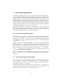
A constraint programming model [3] is proposed as a method to automatically find a
good solution for aiding the programmer installing and configuring the FRIDA robot
in an assembly environment and thus decreasing setup times and cycle times simultaneously.
1.2
Project Purpose and Goal
The purpose of this project is to evaluate the suitability of using constraint programming on robotic assembly sequencing. The problem is modelled as a vehicle routing
problem [16] with a set of constraints adding the restrictions to the robot which are not
in the standard vehicle routing problem.
The aim of this project is to implement a constraint programming model for solving the
problem as a vehicle routing problem and benchmark it against real-life installations.
7
An actual installation of the FRIDA robot cell has been used to generate a test case. In
this installation a skilled engineer has achieved a good cycle time; this time is used as
case benchmark. This reference installation was made within a timespan of a couple
of weeks. The constraint programming approach will be applied on the same setup to
achieve comparable results.
1.3
Scope
In the thesis project the focus is to demonstrate a constraint programming solution to
find good sequences for one FRIDA robot; solutions are not required to be optimal but
good enough. The solution will use a fixed tray layout in the production cell, meaning
that no changes in the geographical layout are done. These trays are the same as in the
reference installation. To automatically find good solutions, the product components
will have the possibility to be moved between these fixed trays instead of moving the
actual trays.
The model will take into account collision avoidance by disallowing certain trays, fixtures and cameras to be visited by both arms simultaneously. To avoid this, waiting is
allowed at trays, fixtures and cameras.
The constraint programming model does not utilise the kinematics or dynamics of the
robot, but instead uses travel times and operation times generated off-line, obtained by
simulation in Robot Studio.
1.4
Structure of the Report
The rest of this report is structured in seven sections.
Section 2 deals with the details of the problem and the background of ABB. It presents
the FRIDA robot in more detail as well as the robot’s working environment.
An introduction to the vehicle routing problem and an outline of the research that have
been conducted on this specific problem type are given in section 3. It introduces some
variants of the vehicle routing problem and popular approaches to solving them. The
job shop problem is also introduced since it is closely related to the vehicle routing
problem.
Section 4 introduces the constraint programming paradigm and Google OR-Tools, the
constraint programming library used to implement the model used in the thesis work.
This section contains the theoretical background to understand the proposed model
described in the thesis.
A description of the implemented constraint programming model is given in section 5.
The model is presented in detail together with core constraints for the vehicle routing
problem and the implemented constraints to solve the specific demands of the scheduling problem with the FRIDA robot.
Results of the constraint programming model are presented in section 6 of the report.
It compares running times and solution quality of some combinations of constraints
and search strategies as well as the reference solution’s cycle time. A comprehensive
description of the setting for testing is given in this section.
8
Section 7 contains the analysis of the results and conclusions drawn from these results.
These results are further discussed in section 8 where future work containing improvements and alternative modelling techniques that might be interesting are proposed.
9
2
2.1
Background
ABB Robotics and the FRIDA Robot
ABB is one of the leaders in robotics technology for industrial applications. Since the
first electrical robot was introduced the number of ABB robots used in industry has
risen to around 160,000 all over the world [2]. The areas of application for such robots
range from painting of components to welding, polishing and grinding. One major
improvement for industry is the possibility to use robots for heavy and monotonous
duties such as lifting heavy components.
Robotics is used all over the world and in many industries, from computer manufacturing to buildings cars, and the most beneficial part of integrating robots in the work
flow is to improve the working conditions for humans. However most robots are big
and working in the same area as a robot requires special safety conditions to be met to
ensure a safe environment.
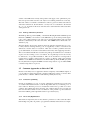
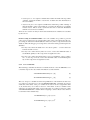
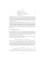
The Flexible Robot Industrial Dual Arm (FRIDA) shown in Figure 1, is a concept robot
designed by ABB to meet the demands of agile production environments that are usually found in manufacturing of consumer electronics [19]. Although the robot is made
for cooperating with humans or other robots, this thesis will only handle the situation
where a single robot is working alone in an isolated environment with a dedicated input
and output area for components and assemblies.
Figure 1: Two FRIDA robots working on an assembly line.
The robot prototype is composed of a portable two-armed robot that is the same size
as an average adult human. The robot’s arms contain 7 rotating joints which allows
the robot to work within spaces that are designed for human working conditions, or
even more confined spaces. Another part of the concept is that it is completely safe to
share workspace with the robot, as it does not require specific safety regulations. This
is useful when an assembly can utilise the parallelisation that the robot is capable of
and the precision of a human coworker.
To perform duties similar to those of a human worker, the robot is fitted with hands.
In the case study the hands consist of two suction tools for picking up flat components
and a gripping tool for pick ups and performing other tasks such as lifting trays.
2.2
Assembly Graphs
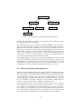
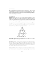
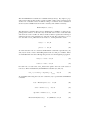
The description of how to assemble a product is called an assembly graph, giving the
break-down of the assembled product and the order in which the components are as-
10
Product Assembly
Sub-assembly
Process Operation
Process Operation
Component 2
Component 3
Component 1
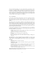
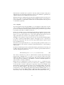
Figure 2: An example of how an assembly graph is represented.
sembled. This graph will also contain process steps that must be performed before the
next step in the assembly can take place.
An assembly graph gives the programmer installing the FRIDA robot a relation between the components and the ordering of each part of the assembly. When programming the robot it is the basic algorithm for how to perform an assembly of a product.
Figure 2 shows an example of an assembly graph containing three components on two
sub-assemblies. In order to achieve a correct assembly, component 1 and component
2 need to be assembled before component 3 can be added and finishing the product
assembly. Also, component 1 and 3 are subject to some process operation which needs
to be performed before they can be added to the assembly.
The assembly graph is represented as a tree with the assembled product as the root and
possible sub-assemblies as sub-trees; the leaf nodes are made up by the components in
the assembly. Since each branch of the tree can be made in parallel, there is not a total
ordering between operations as long as the robot has capacity for the task, e.g. one arm
can pick up one component while the other arm can perform a process step.
2.3
The Lean Production Environment Cell
The production environment in which the robot is placed when working with product
assembly is called a cell. Within this cell the FRIDA robot is operating autonomously
without any interference from the outside world. The input is trays with new parts,
or sub-assemblies, to assemble. The output are those parts assembled to a new subassembly. The input trays are filled outside the cell by a different part of the production
line, be it manually or automated. The given output assembly is handled either by
another robot in the production line or manually by a human worker.
The components that the robot will assemble are initially laid out on trays in the cell
from which the robot will pick up components and place them on one or several fixtures. A fixture is a mounting for a sub-assembly which gives the robot a stable reference where the components always are positioned in the same way. The layout of these
trays and the fixtures is flexible and can be moved anywhere inside the cell. Also each
tray is of the same size, which allows for several combinations of the cell layout.
11
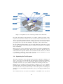
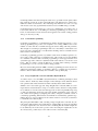
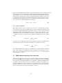
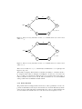
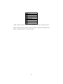
Figure 3: A simplified overview of the lean production environment cell.
For each component tray in the cell there is one camera. To find components on the
tray the robot system uses cameras as its vision system. These cameras are also used
when a component is picked up using the suction tools; the robot knows the placement
of the component with a minor error. To compensate for this error it needs to take a
photograph of the component and calculate at what angle to place it at the fixture.
In some applications there might be other tools in the cell that are required for a certain
process step, examples of this are air-guns for cleaning components before assembling
them on the fixture.
Figure 3 gives an overview of the layout of the cell in the case study as simulated in the
programming software, Robot Studio. The trays are positioned so that the robot can
easily reach each component and there are two fixtures in front of the robot on which
to assemble the components. The cell also contains 5 cameras distributed over each
tray and an air-gun in the upper left corner of the cell.
2.4
Optimising the Task Sequence
The many combinations of the cell setup together with the complexity of finding good
ways to move the robot’s arms through the cell requires experienced programmers.
Since each assembly is to be done several times during a product’s life time, each
assembly is referred to as a cycle, with the assembly line containing several cycles.
Finding the robot assembly sequence under these conditions proves to be a difficult
task and requires experienced programmers who know what can be done to improve
the total cycle time of the product assembly. Even with experience, installing and
getting a robot to run can take several weeks to get a good enough performance from
the robot.
In the studied reference case where an installation of the FRIDA robot was carried
12
out, the time it took for the entire installation to reach good enough results was a
couple of weeks. This project was made by an ABB engineer who manually crafted
the sequences in which the robot would carry out certain tasks and optimisations were
done in small iterations.
In order to save time and to get the most out of the FRIDA robots when automating a
product assembly this process of installing and configuring the robot could be done by
using operations research tools to automatically construct robust assembly sequences;
and search for an optimal task sequence.
As an addition to the finding of an optimal task sequence the tools can also be used to
identify bottlenecks in the design of the production cell and in that way aid an iterative
process of continuously optimising the installation.
13
3
3.1
The Vehicle Routing Problem
The Travelling Salesperson Problem
The Travelling Salesperson Problem (TSP) is a specialisation of the vehicle routing
problem and is one of the oldest optimisation problems known. The problem is formulated as Find the shortest path a salesperson can take to visit all of his customers in one
route and return to his home town. The goal can be reformulated as finding a Hamiltonian tour given a set of nodes in a complete graph [8]. Formally the problem can be
defined as given a set of N nodes and a distance Ci j which represents the distance of
the edge from node i to node j; if the edge does not exist, this value is either infinity or
the shortest distance between i and j depending on the problem. A solution is a path of
N edges forming a circuit.
3.2
Generalising the TSP
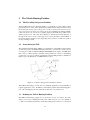
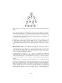
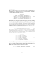
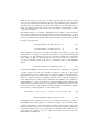
The Vehicle Routing Problem (VRP) is a generalisation of the TSP. Consider adding
several salespeople to the TSP such that the problem is to visit all nodes exactly once by
one salesperson. This is called the Multiple TSP (MTSP) and is equal to the VRP when
there exist no vehicle capacity constraints. The problem now consists of distributing
several visits over a set of vehicles such that the total travelling distance is minimised;
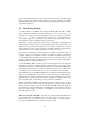
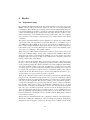
Figure 4 gives an illustration of a VRP with three routes.
Figure 4: A vehicle routing problem with three vehicles.
The VRP is interesting in several ways for industrial applications and specifically in
logistics applications. Also, the TSP is a well-studied problem with industrial application, such as finding the shortest path between all nodes on a circuit board.
3.3
Defining the Vehicle Routing Problem
The VRP is defined using a graph G = (V, A) where V is a set of n vertices, the visits,
and A is a set of arcs combining all vertices in V . With every arc ai j a cost is defined as
ci j . This cost can differ in different contexts but is interpreted as the travel cost between
14
nodes i and j. We also define a set of m vehicles with routes Rk 2 {R1 , R2 , . . . , Rm }, that
together cover all visits [16].
A solution to the VRP is to assign all nodes v 2 V to a route Rk such that
• Each node Vi , except the depot, is visited exactly once.
• All vehicles start and end at a fixed depot that is visited once by each vehicle.
• Side constraints are satisfied.
The objective of the VRP is to minimise the travelling cost over all vehicle routes.
Finding an optimal route is NP-hard [22, 18, 15, 4]. Sometimes additional objectives
are added to the problem, a common objective is to minimise the number of vehicles
used to perform all visits.
3.4
Variations of the VRP
Except for the pure VRP there is a large amount of variations where specific side constraints are enforced. These side constraints range from time based constraints to route
based constraints and even constraints on certain visits.
Apart from these well-studied academic variations, in industrial applications the VRP
is composed of combinations of all variations and affected by real-life side constraints
such as working hours for chauffeurs and compatibility between customers. These
combined VRPs are called Rich VRPs, since they express several constraints and parameters from several VRP variations that further increase the difficulty of the problem.
3.4.1
Capacitated Vehicle Routing Problem
The capacitated vehicle routing problem (CVRP) is perhaps the most common variant
of the VRP, sometimes the VRP is defined as the CVRP. It adds the notion of goods that
need to be distributed to the nodes in the problem. For each vehicle a capacity is defined
and for each customer visit, a demand is defined. A positive demand indicates that a
vehicle needs to deliver the specified amount of goods to the customer; special capacity
constraints where customers can have negative demands are described in Section 3.4.3.
Depending on the problem, the vehicle fleet can be heterogeneous or homogeneous,
meaning that the capacity of each vehicle is either unique or identical. Apart from the
fleet being heterogeneous or homogeneous, each vehicle can carry either one or several
goods, up to its capacity.
The objective is the same as in the original VRP with the added constraint that the cumulative demand on a vehicle route Rk cannot at any node exceed the vehicle’s capacity
Qk .
3.4.2
Vehicle Routing Problem with Time Windows
Vehicle routing problems with time windows (VRPTW) are another variation, which
is most common in industrial applications and other applications, such as home care
scheduling. It adds specific time intervals where the customers can be served. This
15
variant of the VRP arises in many transportation and supply route optimisation problems. It is present when customers can only be served during certain hours of the day.
The time window constraint is formulated as follows; given an earliest start time Ei
and a latest start time Li , the arrival time ai for any node i is constrained to the interval
Ei  ai  Li . A vehicle is allowed to wait if it arrives earlier than the earliest start time
of the given node.
3.4.3
Pick-up and Delivery Problem
The Pick-up delivery problem (PDP), or the Vehicle Routing Problem with Pick-up and
Deliveries (VRPPD), is an extension of the VRP where goods are transported along the
route of any vehicle such that some visits are associated with pick-ups and some with
deliveries, alternatively both at the same time. The VRPPD can be divided into two
subclasses [18].
The first subclass involves the situation where the pick-ups and deliveries are a oneto-many relation, meaning that the goods are supplied by a subset of customers and
delivered to another subset of customers. This class considers problems where the
goods demanded at one customer can be delivered from any of the supplying customers.
The second subclass handles the case where the pick-ups and deliveries are constructed
as pairs of nodes, forming a one-to-one relation. Goods picked up at one node can only
be delivered to one specified destination. This can be described as a transportation
request where a packet is transported via a route to a delivery. This is the classical
definition of the PDP and is identical to the Dial-A-Ride problem (DARP) [18] with
the only difference being that the PDP considers transportation of goods while DARP
considers transportation of persons.
3.5
Common Approaches to Solve the VRP
Because of the many areas of application and the complexity of the VRP, the impact of
a good solution is huge and can help companies make large savings or increase their
profit. Because of this the VRP is a well-studied problem [16, 24, 14].
3.5.1
Genetic Programming
Genetic programming is a way of solving optimisation problems based on the idea
of evolution and natural selection. Such an algorithm starts by constructing a set of
naive solutions. Then the process is to mutate this solution into a possible set of other
solutions and evaluate their fitness keeping only solutions that are strong enough. In
this sense the fitness function is the cost function of the problem e.g. the total travel
time in the VRP. A genetic algorithm solution is presented in [22].
3.5.2
Ant Colony Optimisation
This method is inspired by ant colonies and ants’ preference to follow other ants rather
than finding new paths. In practice a program that simulates this behaviour is imple16
mented. It is utilised by finding a set of routes with ant agents, representations of ants,
to generate a set of initial solutions. After the first set of solutions are found, the total distance is calculated over all routes and the one with the lowest cost is saved as
a pheromone trail. When the ant agents search the graph and select which node to
travel to next they use a probabilistic rule and prefer to move to a node based on short
edges or high pheromone value. Ant colony optimisation has been successfully used in
solving the TSP [12] and is applicable to the VRP [21].
3.5.3
Local Search
Local search is a meta-heuristic technique that is often used for optimisation problems.
This technique defines a transition function that given one solution will explore the
neighbouring solutions that can be reached from the initial solution via the transition
function.
The objective value of the problem is evaluated for each neighbour and only the candidates that improve the current solution the most are kept for further iteration. The
process is then repeated with the optimal solution as the new current solution. Local
search is an iterative improvement method that only finds solutions that are neighbours
of the current solution and can therefore not be sure to find an optimal solution to the
problem: it might only find local optima.
Local search is a popular approach to solve routing problems because of the simplicity
to define the neighbourhoods of a route. For solving routing problems with local search
there exist several move operators [15]:
• 2-Opt, change the location of two arcs in the route. The two arcs are removed
and the nodes affected are connected by new arcs.
• Relocate, move a visit from one route to another route.
• Exchange, swap two nodes between two different routes.
• Cross, exchange parts of two routes. This could be the starting or ending part of
the routes.
The following move operators are implemented in Google OR-Tools, see Section 4.10,
and require the use of Boolean variables to designate if a node is active in the current
solution. This is to model disjunctions where only one visit in a set of customers is
performed:
• MakeActive, make one inactive visit active.
• MakeInactive, make one active visit inactive. The direct opposite to the MakeActive move operator.
• SwapActive, make one active visit inactive while inserting one inactive visit in
the exact same place in the route such that the travel time is reduced.
• Extended SwapActive, equal to SwapActive but test all possible insertions of all
inactive visits when inserting the inactive visit.
Apart from the mentioned local search moves there also exist several others that can be
implemented depending on what problem is to be solved.
17
Certain algorithms exist that can help the search not to get stuck in local optima, rather
they guide the search out of the local neighbourhood in different ways. These algorithms are called meta-heuristics. Two interesting meta heuristics are tabu search [7]
and simulated annealing [9] which have both been used on VRPs with good results.
Constraint-based local search [27] is a concept of combining the speed and power of
local search with the ease of modelling in constraint programming, see Section 3.5.4
below. Constraint-based local search has been applied to the vehicle routing problem
with good outcome [11, 20].
3.5.4
Constraint Programming
Constraint programming is a paradigm that is further described in Section 4. Constraint programming has proven to be a helpful tool in solving VRPs because of the
number of real-world side constraints that appear when working with real problems.
The strength of constraint programming in this case is the ability to with relative ease
incorporate side constraints into a model and the checking of these constraints ensures
that a solution is feasible [15].
Constraint programming performs a systematic search and is normally required to explore each possible solution in a predefined order. The search process and checking
of constraints sometimes make constraint programming a slower approach than nonsystematic approaches, unless it is hybridised with other methods, as in Section 3.5.5
below. This is a matter of trade-off that has to be made when selecting constraint
programming as a tool to solve the vehicle routing problem.
However when dealing with rich VRPs constraint programming has been shown to be
efficient in reducing the number of candidate solutions to evaluate since it guarantees
that the solutions returned all satisfy the constraints of the problem [20].
3.5.5
Large Neighbourhood Search and Other Hybrid Methods
A common way to solve the VRP is by hybrid methods, combining techniques to find
better solutions. In this way all the strengths of the techniques can be utilised to find a
near-optimal solution fast and with reasonable certainty that it will be feasible.
Similar to the local search approach, Large Neighbourhood Search (LNS) is a technique that uses meta-heuristics to improve a current solution. Instead of using smaller
moves like those in local search, the LNS approach is aimed at gradually improving
a solution by alternately destroying (removing variable assignments) parts of the current solution and repairing it (assigning new values) using the systematic search of
constraint programming. The heuristics used in LNS are such that they guide the algorithm in these two steps by telling how the current solution is to be destroyed and how
to rebuild the next solution [20].
The principle behind LNS is that searching a larger neighbourhood around any current solution will result in local optima that are of high quality; however the searching
of a larger neighbourhood is often more time consuming than the smaller neighbourhoods defined by the local search operators since increasing the neighbourhood size
also increases the possible ways a new solution can be constructed [20].
18
Several other hybrid approaches have been introduced and show promising results
when solving the pure vehicle routing problem types; such an example is to combine
different meta-heuristic methods such as genetic programming with simulated annealing and tabu search [23].
3.6
The Job Shop Problem
A problem similar to the VRP is the Job Shop Problem (JSP). The JSP is an NPhard combinatorial optimisation problem described by a set J of jobs that are to be
scheduled over a set M of resources [30]. Each job consists of a sequence of activities
A = [a1 j , a2 j , . . . , ai j ] where ai j represents the ith activity of job j 2 J. Each activity ai j
corresponds to a pair (mi j , pi j ) where pi j is the duration for the activity and mi j 2 M is
the designated resource on which the activity is performed.
Each activity requires an allocated resource for the entire duration, meaning that no
other task may be using the same resource during that time. Also all tasks have to be
finished once they are started, meaning that no pre-emption is allowed. The ordering
of the activities for each job posts precedence constraints such that no activity may be
started before the previous activity has finished executing on a resource.
The problem is modeled by posting disjunctive constraints on all activities that use
the same resource and conjunctive constraints on activities in each job such that the
complete ordering is preserved. The objective of the JSP is to minimise the makespan
of the schedule, that is the time passed between the start of the first activity on all
resources and the completion of the last activity on all resources. This is equivalent to
minimising the time of the last finished job.
As with the VRP the JSP is not always as pure as the description above. In real-world
applications several side constraints must be considered and it is not as strict. There
is examples where there are additional transition times representing the minimum time
that must pass between any two executions on the same resource. It is not uncommon
for activities to be associated with a set of resources on which it can be scheduled.
The similarities between the VRP and JSP have been studied in the literature and techniques for reformulating the two problems into each other have been studied and presented with good results [4]. This shows that there is great similarity between the two
problems and most of the real applications have elements of scheduling and routing
such as travelling time, total ordering of visits or activities, and duration.
When reformulating the VRP as a scheduling problem the vehicles become resources
and the visits become activities that are to be performed on these resources. Each
activity can be performed on each resource and when the VRP contains time windows,
the execution is constrained within these. Travelling times are remodeled as transition
times. To model capacities on vehicles, a consumable second resource is associated
with each primary resource.
When to use the JSP or the VRP Since there are several problems that fall between
the pure JSP and the pure VRP there have to be some criteria to determine what solution method to use to solve these grey-zone problems. Beck et al. [4] present some
properties that differentiate the two problems from each other.
19
• In the VRP the duration of operations at each node is small compared to the
transit time, however in the JSP the operations are dominant.
• In the JSP the objective is to minimise the ending time for the last task, also
called makespan. In the VRP the studied criterion is the travel time over all
routes.
• In the JSP, there are usually few resources that can perform an activity, in the
VRP, on the other hand, most vehicles can perform most visits.
• The JSP has time window dependencies that are fixed for all activities. The task
is to allocate a resource to each activity. The VRP contains fewer dependencies
between visits, especially on different routes.
In another study by Beck et al. [5] the similarities and differences of the VRP and
JSP are examined. The experiments in the study are done by solving a test instance
generated from attributes which range from VRP properties to JSP properties. These
instances are solved using JSP solvers using systematic search and VRP solvers using
local search. The result presented shows that both solvers are able to solve all instances
to optimality. However when several precedence constraints are present the VRP solver
must begin with a solution from the JSP solver in order to find an optimal solution.
3.7
The VRP of the Thesis Project
The FRIDA sequencing problem in this thesis project is formulated as a vehicle routing
problem with pick-ups and deliveries together with several side constraints. The goal
is to find a sequence of visits that satisfies all these constraints to assembles the product
correctly.
In the thesis VRP, each task to be performed is a visit node; this can be pick-up of
a component or photographing to compensate for errors in the pick-up. Vehicles in
the thesis VRP are the robot’s hands. The routes are the ordering in which the robot
assembles a product.
Each component will have exactly one pick-up node and one drop-off node with at least
one additional process operation, such as cleaning a component before the drop-off or
removal of adhesive tapes after drop-off.
Because of the assembly graph and the ordering of the product assembly, there exist
numerous precedence constraints. These constraints present themselves both on each
component’s individual nodes as well as between the drop-off of all components together.
Time windows represent work-time of each node, and these are used to separate work
that cannot be performed at the same time.
Depending on the input assembly graph and number of components, the size of the
thesis VRP lies in the range of a medium-sized problem as described by Caseau and
Laburthe [8] meaning that the size ranges from 30 to 90 nodes and therefore motivates
the using of constraint programming. Being rich further increases the difficulty of the
problem.
Some of the attributes of this problem lie in the domain of a JSP, such as the precedence
constraints. The choice of modelling as a VRP comes from the remaining attributes
20
being dominant in that the travel time between the trays, fixtures and cameras is greater
than the duration to perform the pick-up or drop-off operations.
21
4
Constraint Programming
Constraint programming (CP) is a way to solve problems through modelling the problem as a Constraint Satisfaction Problem (CSP) with variables and constraints describing relations between variables. The CP paradigm is declarative, meaning that as a programmer the task is to describe the problem’s structure and the logic without control
flow. The problem model contains all information necessary to solve the problem with
a general algorithm, parametrised by inference algorithms that are specific to the constraints used in the model. This allows the flexibility of reusing the general algorithm
for many different problems. The software implementing the constraint programming
algorithms and constraints is here referred to as the solver.
This section introduces the necessary theory and definitions needed to understand the
implemented model and the discussions sections of the report. This section is based
on [3, 25] , the interested reader is encouraged to read them for further information on
constraint programming and examples of other problem types.
4.1
Constraint Satisfaction Problems
Constraint satisfaction problems are defined as CSP = hV, D,Ci where D(vi ) represents
the domain for each variable vi 2 V , i.e. D(vi ) contains all possible values that can be
assigned to vi . A constraint c 2 C on a subset Vn ofV is a relation that restricts the values
of the variables Vn . If |Vn | = 1 then the constraint is a unary constraint. Examples of
constraints are x > y or x 6= 1.
A CSP is considered solved when all variables vi 2 V have been assigned values such
that all constraints c 2 C are satisfied. This is the process of propagation and search
that assigns and removes values from variable domains. If all constraints are satisfied
and some variables have multiple values in their domains, this is called a general solution. The solutions are a subset of the Cartesian product D(x) ⇥ · · · ⇥ D(y), where
V = {x, . . . , y}. This gives a set of allowed combinations of value assignments for all
v 2 V such that all constraints are satisfied.
The store of the CSP solver is all the variables together with their current domains.
This is needed for the solver to keep track of the global state of the problem when
solving it.
4.2
Constrained Optimisation Problems
A constrained optimisation problem (COP) is defined as a CSP with an objective function f from D(x) ⇥ · · · ⇥ D(y) to a number, where V = {x, . . . , y}. The goal of a constrained optimisation problem is to find a solution such that all constraints are satisfied
and such that the value of f is optimised.
Solving a COP by branch-and-bound introduces the objective as a constraint that for
each feasible solution n the value must be lower than the current best value b, for a
minimisation problem, and higher for a maximisation problem.
22
4.3
Propagation
One of the central concepts in CP is propagation. Propagation is the process of removing values from the domains of variables given that the assignment of the value
will lead to an infeasible solution. The disallowed values are pruned from the domain.
For some constraints it is straight-forward to find what values will be pruned from the
domain, such as for the constraint x > 5 for any variable x: all values that are less than
or equal to 5 will be removed from the domain of x.
A propagator is the implementation of a constraint and is responsible for monitoring
the values of variables covered by the constraint and removing values which break
the constraint. The purpose of the propagator is to strengthen the current store into a
stronger store. A store s1 is stronger than another store s2 iff s1 (x) ⇢ s2 (x) for at least
one variable x. This denotes an ordering amongst stores and is written as s1 s2 (we
say that s1 is stronger than s2 ).
When changes occur to the domain of any variable in the store of a constraint the
propagator may prune further values which break the constraint it implements. In other
words the propagator will remove values that cannot be a part of the solution under the
current store. A propagator is said to be at fixpoint when it cannot remove any more
values from the current store.
If at any point, the propagator finds that any value to the variables in the store is not
violating the constraint and can appear in the final solution, we say that it is subsumed.
A subsumed propagator does not have to check the store for any change to the store
later in the solving process.
However if the propagator prunes a domain to an empty set it will fail. In this case the
constraint is violated under the current store and no feasible solution exists.
4.4
Consistency
Once the propagation algorithm has finished, it is said to have reached consistency.
This consistency is the termination criterion for the algorithm and specifies that under
the current store, there exist values in the domains of the covered variables such that
the constraint is satisfied. If the propagator signals a failure the store is said to be
inconsistent. This notion of consistency is vital in constraint programming and is well
researched in the literature. There are several levels of consistency but two of the most
common are domain and bound consistency.
Bound consistency is reached whenever for a constraint c and all its variables xi the
bounds of xi participate in a solution to the constraint c. This level of consistency is
efficient when dealing with linear inequalities, such as x < y.
Domain consistency is defined such that for a constraint c and all its variables xi , for
each value in the domain D(xi ) there exist values in the domain of all other variables
in c such that all the values form a solution to c. This is the most popular and strongest
consistency level and is often referred to as Generalised Arc Consistency (GAC). To
achieve GAC is expensive and sometimes the cost of reaching GAC is not motivated
and thus a weaker consistency is chosen instead.
23
In order to tune the solving process, different levels of consistency are usually experimented with so as to find a solution fast. In the VRP there has been evidence where
using bound consistency for some constraints will increase the speed of the search process and aid in finding better solutions within some given time limit. This time limit
is usually present in situations where a good enough solution has to be found fast;
however it is not necessarily optimal.
4.5
Search
Only propagation in itself is not enough to find a solution, instead the solver needs
to search for solutions. Together with propagation, the search is the main concept for
constraint programming. The search made by the constraint solver is a complete search,
meaning that it will cover all possible assignments of values to variables.
Propagation occurs in each search step to prune values leading to an infeasible solution
under the current store, resulting in a stronger store. This ensures that the size of the
search space is strictly decreasing. Without propagation during search it would be
reduced to a brute-force search. Constraint propagation together with the complete
search is what makes constraint programming a powerful tool.
4.5.1
Branching
In constraint programming, the search space is defined as a search tree. This tree is
defined by the branching of the model and guides the search for solutions to the current
application.
The branching is what defines the search tree by selecting variables which are not yet
assigned values after propagation and dividing their domain into at least two non-empty
and non-overlapping partitions. Each partition is a decision on what values the variable
can be assigned in a possible solution. The decision creates a branch in the search tree
and defines the store for each of the resulting sub-trees. Note that the root of the tree is
the store after initial propagation, and each leaf node is either a failure or a solution.
After each decision, the affected propagators will check that the current store is consistent with each propagator and prune values if possible. If all propagators are subsumed
at this point, all combinations of assignments in the store are solutions. If any propagator signals a failure the current store and that subtree of the search will not contain any
feasible solution and the solver will backtrack. When a backtrack occurs, the solver
will undo the latest decision and try with the next partition of the variable domain
instead.
The resulting search tree is finite, with suitable conditions on the branching, since the
store after each propagation is stronger than the previous. It is non-overlapping such
that no solution to the problem is duplicated. And the solver does not lose solutions
during search, rendering a complete search over all assignments. It is also systematic,
only considering one variable at each decision until all variables are assigned.
24
4.5.2
Heuristics
How to branch during search is defined by the branching heuristics. These are based
on the programmer’s knowledge of the search space and the problem at hand. These
heuristics define in what order the variables are selected for branching and what decisions (e.g., value assignments) should be done in each branch. Branching heuristics are
vital in order to find good solutions fast.
4.5.3
Exploration
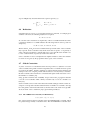
Depth-First Search One way to solve constraint satisfaction problems is to use a
depth-first search (DFS) approach. The search will explore each branch as deep as
possible before backtracking. If a propagator fails at any node the search will backtrack
and try the right branch before continuing on the left branch until a solution is found.
An example of DFS is given by Figure 5 that shows that the left-most nodes of the tree
are visited first, then the search systematically visits the closest branch to the right.
This approach is common in constraint programming since in many cases it will lead to
finding a solution fast given that the constraints propagate well such that backtracking is
minimised. When solving CSPs each leaf node of the search tree is a possible solution,
therefore DFS is a good choice for exploring the search tree.
1
7
2
3
4
9
6
5
8
10
12
11
Figure 5: The numbering of the nodes designates the order in which the nodes of the
search tree are explored during depth-first search.
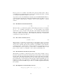
Breadth-First Search Another exploration strategy that can be utilised is breadthfirst-search (BFS). In contrast to DFS the search will explore each level in the search
tree in the order shown in Figure 6. Each level will be completely explored from left
to right before progressing to the next level. BFS is a good choice if the search tree is
such that there might exist solutions at any level of the tree.
Branch-and-Bound When working with constrained optimisation problems, branchand-bound is a common choice for exploration. It works in the same way as DFS or
BFS with the addition of a boundary function f , computing the upper and lower bound
25
1
3
2
5
9
7
6
10
4
11
8
12
Figure 6: The order in which nodes of the search tree is explored during breadth-first
search.
of the objective function in the COP. For every decision made during the search, the
best value of that branch for f is evaluated. If the new bound is lower than the previous best the branch is further explored. Otherwise the entire subtree under the branch
is pruned from the search space and the solver will continue on the next branch, or
backtrack if no other branch exists.
The function f can be any function that, for the given problem, calculates a good
boundary value. This function could be strictly discrete or it can be a relaxed to a
real-value function. For vehicle routing problems, a good boundary function to use is
a shortest path heuristic function that can compute the best bound for each route in the
VRP.
Restarts During Search Assume that the branching uses randomisation. The cost
of backtracking can be too high and to save time during the search a restart strategy
can be implemented. This restart is set to start the search from the root node once a
criterion has been met. This criterion can be a time limit, no solution found within x
seconds, or a limit on the number of failures.
A restart strategy is a sequence (t1 ,t2 ,t3 , . . . ) where ti is the number of branches and
backtracking steps the randomised search is allowed to perform. After ti steps, the
search is restarted from the root node and is allowed to run for ti+1 steps. The sequence
can either be the number of steps or a sequence of scalars multiplied by a fixed number
of steps.
Restart strategies are commonly used for minimising the cost of randomised search
heuristics. As with all heuristics, the restart strategy selected is based on knowledge of
the problem at hand. In the case of randomised search it is based on the run-time distribution of the specific problem; these strategies are called non-universal. In contrast,
universal strategies are used to work with any problem. The first proposed universal
strategy is the Luby sequence [17] to solve problems with randomised algorithms. The
Luby sequence is given by S = (1, 1, 2, 1, 1, 2, 4, 1, 1, 2, 4, 8, . . . ) where the number of
26
steps is multiplied by the ith element in the sequence given by (1).
ti =
4.6
(
2k 1 ,
ti 2k 1 +1 ,
if i = 2k 1;
if 2k 1  i < 2k
1.
(1)
Reification
Sometimes there is reason to post a disjunction between constraints, for example given
variables A, B and C, the following disjunction is required.
A + B = C _C = 0
To solve this each constraint is accompanied by a Boolean variable that indicates if the
constraint is satisfied or not. With reification the following relations can be posted in a
simple way:
A + B = C $ b1 , C = 0 $ b2 , b1 _ b2
The Booleans b1 and b2 are decision variables that represent the status of the constraints
they represent. If the constraint holds, the Boolean value is equal to 1, respectively a
value of 0 represents that the constraint fails. Vice versa, if the Boolean variable is set
to 1 the constraint holds, respectively it fails if the value is 0.
Some constraints in solvers can implement an implicit reification, where the variables
b1 and b2 are not given by the programmer but as a part of the constraint.
4.7
Global Constraints
A global constraint is a constraint that can be decomposed into a conjunction of several
other constraints. The global constraint encapsulates these constraints and uses special
propagation algorithms. Global constraints are well documented in the literature and
often proved to solve complex problem which cannot be solved by binary constraints.
Global constraints can be described as constraints that capture relations between a nonfixed number of variables [28].
Using global constraints adds readability and provides better propagation that will
cover all covered variables while a binary constraint only covers two variables at a
time [28].
Such constraints can be found in the Global Constraint Catalogue which contains descriptions of 347 global constraints and their names in a number of constraint solvers [6].
For each global constraint described below, the first name is the name in Google ORTools, the name of the constraint in [28] is given within parentheses.
4.7.1
The AllDifferent Constraint (A LL D IFFERENT)
8 xi , x j 2 X : i 6= j ! xi 6= x j
(2)
One of the best known global constraints is the A LL D IFFERENT(X) constraint, which
has practical usage in many constraint models. The A LL D IFFERENT constraint states
27
that in a given set of variables, all variables have pairwise distinct values. This is
a straightforward constraint that can be expressed by declaring the binary constraint
xi 6= x j between all distinct variables xi and x j of X.
A special case of the A LL D IFFERENT constraint is the A LL D IFFERENT E XCEPT(X, c)
constraint which works like the standard A LLDIFFERENT with the addition of a constant c and the condition that two variables xi and x j can be assigned to c without
violation.
4.7.2
The Element Constraint (E LEMENT)
z = X[y]
(3)
The Element(X, y, z) constraint is a global constraint that given an array of n variables
X = [x1 , . . . , xn ], a variable y where D(y) ✓ {1, . . . , n}, and a variable z, the constraint
enforces that z = X[y]. In other words: the value of the variable in X indexed by the
value of y is equal to the value of z. Alternatively this constraint could be used with
a constant c instead of the variable z. The variable in X indexed by y would then be
constrained to be equal to the value of c.
4.7.3
The Count Constraint (C OUNT)
|{x 2 X | x = v}| = c
(4)
The C OUNT(X, c) constraint, as represented in (4), states that the value v is present in
variable array X, exactly c times. This is useful for modelling problems where there
exist resource constraints. The C OUNT constraint is a specialisation of the Distribute
constraint (GLOBAL _ CARDINALITY), which is defined as an aggregated version of
C OUNT that takes a set VC of pairs (v, c) and an array of variables X. Then for each
pair (v, c) in VC, value v is constrained to occur c times for all variables in X.
4.7.4
The Transition Constraint (I N _R ELATION)
The Transition constraint is commonly also known as the table constraint or the extensional constraint. An extensional constraint expresses the relation of that constraint
through a table. The table will explicitly tell the propagator what subset of the Cartesian product of the variable domains is allowed. In contrast usual constraints calculate
the possible subset of the Cartesian product through a dedicated algorithm [13]. Alternatively the table can be replaced by a deterministic finite automaton (DFA). The
regular expression that the DFA accepts is the set of variable assignments that satisfy
the constraint.
4.7.5
The Disjunctive Constraint (D ISJUNCTIVE)
8(si , ei ), (s j , e j ) 2 T | i 6= j : ei  s j _ e j  si
28
(5)
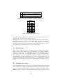
The D ISJUNCTIVE(T ) constraint is a common constraint in scheduling. It ensures that
a given set of tasks, T = {(si , ei ), . . . }, is non-overlapping. By non-overlapping each
task’s start and end times are constrained so that no task starts during another task as
seen in (5). This is illustrated in Figure 7.
Figure 7: The tasks 1, 3, and 4 are disjunctive, i.e. non-overlapping.
In Google OR-Tools, the disjunctive constraint also contains a sequence variable, which
holds a representation of the ordering in which the tasks covered in the constraint are to
occur. This sequence variable is a decision variable used to preserve the order of tasks
scheduled by propagation and is useful when combining the disjunctive constraint with
ordering constraints.
4.7.6
The NoCycle Constraint (C IRCUIT)
The N O C YCLE(N) constraint ensures that for a set N of nodes there exists only one
circuit visiting all nodes. In routing problem this constraint is used to ensure that a
route can only start at the depot start node and end at the depot start node; effectively
eliminating possible sub-tours. This constraint has been shown to be useful in solving routing problems in order to make sure that there exists only one cycle for each
route [15, 8].
The N O C YCLE constraint is very similar to the A LL D IFFERENT constraint in that all
nodes in the graph require a unique successor and predecessor. The different solutions
satisfying this constraint are all the permutations of circuits over the nodes in N.
Even though the constraint name says that no cycles, the outcome of the semantics
described above suggest that it is actually one cycle. Therefore the name C IRCUIT is
more precise since the semantics says exactly one cycle. However the name of the
constraint as used by Google OR-Tools is N O C YCLE.
4.8
Large Neighbourhood Search
A common hybrid approach is to use constraint programming only to control the feasibility of neighbouring solutions found by a local search algorithm [11], also see Section 3.5.5. In this case the search is controlled by the local search and the constraint
model is only used as a checker. It can be done to certain degrees since the cost of
propagating constraints can be high, to the point where it is unacceptable.
When using the constraint model as checker, the local search will be used to find a
candidate solution to a sub-problem which is checked by the constraint solver. Some
implementations of this approach allow using a constraint solver to do the last assignments of variables in a solution found by local search.
29
4.9
Interval Decision Variables
The variables used in a model are decision variables, which are assigned values. The
most common variable is the integer variable. Such a variable is the standard finitedomain variable which can be assigned integer values.
Some solvers contain specialised variables that can be used specifically to solve certain problems. One such variable is the interval variable. An interval variable is a
variable which encapsulates several boundaries: these are useful for modelling tasks
in a scheduling problem. An interval variable can be decomposed into several integer
variables which are constrained with binary constraints.
An interval variable I contains the following integer variables:
• StartI is a variable for the starting time of the interval.
• EndI is a variable for the end time of the interval.
• DurationI is a variable for the duration of the interval. This is the difference
between EndI and StartI . It can either be a variable duration that is to be set
during the solving process, or it can be a fixed duration determined by the input
data.
• PerformedI is a variable to determine if an interval is performed or not. An
interval is unperformed if EndI < StartI , meaning it has a negative duration.
Special binary constraints can be posted on interval variables so as to express precedences. An example of such a constraint is the StartAfterEnd(I1 , I2 ) constraint which
will ensure that StartI2 EndI1 . Other variants of this binary constraint also exist,
which allows synchronising the starts or ends of the intervals.
4.10
Google OR-Tools
The constraint programming library used in this thesis work is Google OR-Tools [29],
a C++ library made by Google and available under the MIT license, an open-source
license. The library also contains interfaces to some linear programming and mixed
integer programming solvers as well as a set of implemented algorithms, such as graph
(e.g. shortest path, min flow, max flow) and knapsack algorithms.
The library contains a superset of the global constraints described in Section 4.7 and
implements local search as an alternative to systematic tree search. This allows one to
use constraint-based local search with relative ease by implementing the local search
operators needed to solve the problem. The library also allows concatenating a list
of local search operators in such a way that the search procedure of each local search
operator is launched in the order they are concatenated: the initial solution for each
operator will then be the last solution from the previous operator.
Further, OR-tools has support for Large Neighbourhood Search as well, which is implemented as a local search heuristic that clears a subset of the variable assignments
and builds a new solution using the constraint solver and values of the remaining assignments.
In addition to the implemented constraints and propagators, Google OR-Tools offers
full support for implementing custom constraints and branching heuristics.
30
5
5.1
Implementation of the Constraint Model
The FRIDA Cell Case Study
The following section will describe the unique input instance used to test the thesis
constraint programming model. The parameters presented are those specific to the
case study, however they are presented in a way to preserve generality. This generality allows reuse of the model without extensive alteration in order to utilise similar
assemblies.
Most of the nodes of the VRP model are related to a pick-up or delivery task, for
example picking a component from a tray and mounting it on a fixture. This creates a
relation on such node pairs which present themselves as precedence constraints where
a component has to be picked up before being placed on a fixture. Aside from the
precedences among the component nodes, there also exist precedence constraints on
the ordering of the assembly, more precisely which component is placed first on the
fixture. This is dictated by the assembly graph and is necessary in order to get a correct
final assembly.
In the definition of the VRP, one node cannot be visited several times since this would
contradict the Hamilton circuit of each route in the problem. In the project the VRP
has some nodes which are geographically the same location, one such example is the
fixture nodes. Because of this, the tasks performed on the fixtures are multiplied such
that there exists one node per task and fixture combination. This also introduces another
aspect of the problem as none of these nodes can be visited at the same time as any other
node, i.e., there is a temporal disjunction between visits.
An extra level of freedom is introduced to find more solutions. By allowing the component tray layout of the cell to be rearranged, the total number of tray nodes is derived
from the possible permutations of component tray layout. The number of fixture nodes
is also multiplied by the number of actual fixtures in the cell, so that the best placement
of the components can be found. Since the VRP states that each node in the problem
can only be visited once, the number of cameras needs to be multiplied by the number
of components that needs to be photographed.
Because of the introduced freedom in the problem, there needs to be an efficient way to
handle nodes that are not active in the final solution. Otherwise finding a good solution
or getting a solution that is near optimal will be extremely hard.
The objective function of this problem is the total cycle time of the assembly, which
corresponds to the total makespan of the assembly. However since the travelling times
are greater than most task durations of the problem, it is still modeled as a vehicle routing problem. Some of the used constraints and variables are those which are intended
to use when modelling scheduling problems. However the experiments in Section 6
suggest that they provide a more efficient model when used together with the routing
constraints and enabled synchronisation between the two routes.
5.2
Model
I now describe the core routing model in terms of instance data, decision variables,
constraints, and objective function. All instance data parameters are referenced with
31
the first letter in upper case, while decision variables will be referenced with lower case
letters.
Instance Data The model takes a description of the production cell as an input in
order to post the constraints. This cell description contains information about the total
number of nodes, fixtures, arms, and components in the problem that are all derived
from the input assembly graph. The following parameters are important for the model:
• NbNodes is the number of nodes in the model i.e., nodes corresponding to a tray,
fixture, camera, etc.
• NbRoutes is the number of routes to be scheduled, one for each robot arm, and
one to assign nodes that are not part of the solution, i.e., nodes that are not active.
• NbComponents is the number of components in the product assembly.
• Q jk is the capacity for a given resource j on route k. In the case study, these
resources are the gripper and suction cup capacities on each of the robot’s arms.
These parameters are used to preserve the generality of the model and allow
solving the problem with different resource configurations on the robot arms.
• Ti jk is the travel time from node i to node j on route k. This data is necessary
to find what arm will have the lowest cost when containing the arc connecting
nodes i and j.
For future reference, the following notation is used for some important set of nodes in
the model. They are used for expressing some of the constraints:
• S = {1, . . . , NbRoutes} is the set of indices for the start nodes for all routes.
• V = {NbRoutes + 1, . . . , NbRoutes + NbNodes} is the set of visits in the cell.
• E = {NbNodes + NbRoutes + 1, . . . , NbNodes + 2 ⇥ NbRoutes} is the set of end
nodes for all routes.
• N = V [ S [ E is the set of all node indices in the model.
• N S = V [ S is the set of nodes that have a successor.
• N E = V [ E is the set of nodes that have a predecessor.
For each node the instance data is generated from information about the components
and the actual location that node represents in the cell. For each node the following
integer parameters are known:
• Id is a unique integer, used to references the node in the input array.
• Component is an integer value that references the component handled at this
node; by either a component pick-up, drop-off, photograph, or operation. For
nodes not representing a component this value will be 0; these nodes are the
output and start and end nodes.
• Fixture is an integer value referencing the fixture the node represents. For nodes
not representing a fixture, this value will be 0.
• Tray is an integer value referencing the tray the node represents. For nodes not
representing a tray, this value will be 0.
32
• Camera is an integer value referencing the camera the node represents. For nodes
not representing a camera, this value will be 0.
• Durations is an integer array of length NbRoutes with the time it take to service
the node on each route. A value of 1 means that the node is out of reach on
that route.
• FixtureOrder is an integer value defining the order in which the node is performed if the node is representing a fixture. Drop-off nodes have order 0 while
operations after drop-off have higher values. For nodes which are not drop-off
nodes, this value is always 0.
• SubAssembly is an integer value describing what sub-assembly the node represents. This parameter is derived from the assembly graph.
Apart from the integer values above; each node contains a number of Boolean values
to designate categories of nodes. These Boolean values are useful for selecting what
nodes are covered by a constraint:
• Start, a Boolean value that designates if a node is one of the start nodes.
• End, a Boolean value that designates if a node is one of the end nodes.
• Output, a Boolean value that designates if a node is the output of the assembly.
This is false for all nodes except the last node in the array.
• Operation, a Boolean value that designates if a node is an operation to be performed on a component before its drop-off. In the case study this node is the
air-gun.
Decision Variables All variables are encapsulated in an array and referenced by a
node. Hence the index i denotes a node in the model where i 2 N:
• nexti 2 N is the index of the immediate successor of i.
• routei 2 S is the index of the arm which visits i, or 0 for the unassigned route.
• arrivali 2 {0, . . . , 263
• departurei
1} is the time of arrival at i.
2 {0, . . . , 263
1} is the time of departure at i.
• starti 2 {0, . . . , 263 1} is the time node i is serviced; this allows modelling
waiting upon arrival at each node.
• accik 2 {0, . . . max Q⇤k } is the accumulated quantity of resource k after visit i.
For this case k can either be load on gripper or suction cup tools.
• intervalim is the interval during which the node i can be serviced on route m. This
is an interval variable.
• activei 2 {0, 1} Boolean variable designating if i is active. This is used by some
constraints to ignore nodes which are not active in the current store. Assigning a
node to route 0 is equal to setting it inactive.
• previ is the index of the immediate predecessor of i. This variable is redundant
with nexti , however it is known to improve the model when solving the VRP [15].
33
• routeSequenceim is a sequence variable that contains information about possible
orderings of interval variables of each route. Contains the same information as
the next variables.
• disjunctiveSequence is a sequence variable that contains the possible orderings of
interval variables on the nodes which are covered by the Disjunctive constraints
in Section 5.3.2. This is used to synchronise the visits of each arm. Redundant
with the arrival and start variables.
All nodes are stored in an array in the model and all decision variables are accessible
by the node id.
Pre-Processing of Variable Domains For some variables it is possible to perform
some pre-processing before propagation takes place. The nodes affected by this preprocessing are derived from their attributes such as tray index, component index, and
durations. The following pre-processing can be done in the model given the input node
attributes:
• For any node i where the duration for one route is equal to
from the domain of routei .
1, remove this route
• For any node i where the tray index is not zero, remove the minimum value of
accumulated quantity for the component’s designated resource.
• For any node i where the fixture index is not zero and fixture order is equal to
zero; i.e, the drop-off nodes, remove the maximum value of accumulated quantity for the component’s designated resource.
5.2.1
Core Constraints
The following constraints are the basic constraints needed to solve the VRP. These core
constraints express the route and the information associated with it:
A LL D IFFERENT E XCEPT(next⇤ , |N|)
(6)
A LL D IFFERENT E XCEPT(prev⇤ , |N|)
(7)
The next⇤ and prev⇤ variables should form permutations of N and all nodes have only
one predecessor and successor: the A LL D IFFERENT E XCEPT constraints (6) and (7)
ensure this. The values of the prev variable at the start nodes are assigned the value
of |N| because they do not have a successor. The values of the next variable at the
end notdes are assigned the value of |N| because they do not have a predecessor. The
A LL D IFFERENT E XCEPT constraint allows assigning a value at these nodes which is
not an index in the variable array.
A LL D IFFERENT(next j , N) 8 j 2 N S
(8)
A LL D IFFERENT(prev j , N) 8 j 2 N E
(9)
34
The A LL D IFFERENT constraints are redundant with (6) and (7): they improve propagation and reduce the time it takes to find a feasible solution. The consistency level
of these two constraints can be modified to find good solutions and is evaluated in
Section 6.3; the available levels are bound consistency and domain consistency.
N O C YCLE(next⇤ , active⇤ )
(10)
The N O C YCLE constraint (10) is used to eliminate the possibilities of sub-tours appearing in the solutions. A sub-tour is any circuit that does not start or end at the start
and end nodes of the overall tour. These circuits would be separated from the depot
and thus create new routes which are not visited by an arm. For nodes where activei is
zero, the value of nexti will be that node’s index, i.e., it will point back to itself.
nextprevi = i 8i 2 N
(11)
prevnexti = i 8i 2 N
(12)
To ensure that the route is consistent, the E LEMENT constraints represented by (11)
and (12) are used to create a channelling between the next and prev variables. These
are redundant with each other, although the presence of both strengthens propagation.
routeprevi = routei
8i 2 N
(13)
routenexti = routei
8i 2 N
(14)
For each node i on each route; routei must be the equal to the route of the successor
node nexti . This is maintained by the E LEMENT constraints (13) and (14).
nexti = j $ arrival j = departurei + Ti j,routei
8i 2 N
(15)
To accumulate time along the route, the constraint (15) is posted with an E LEMENT
constraint.
nexti = RouteSequencei,routei
starti = StartIntervali,routei
departurei = EndIntervali,routei
D ISJUNCTIVE(Intervalir ) :
35
8i 2 N
8i 2 N
(16)
(17)
8i 2 N
(18)
8r 2 NbRoutes, 8i 2 N
(19)
Because of the multiple interval variables associated with each node, the constraints (16), (17),
and (18) represent a set of E LEMENT constraints that channel information from the interval variables to the next, start, and departure variables given the assigned route. The
D ISJUNCTIVE constraint (19) is used to constrain the Interval variables for each route
to be disjunctive: this is used for the relation between the ordering of the nodes and the
start and departure variables for each node. The three time domain variables arrivali ,
starti , and departurei allow waiting time at each node:
arrivali  starti
5.2.2
8i 2 N
(20)
Objective Function
The objective function of the case study is the makespan, so that the total cycle time
can be found for the product assembly. However the model has been evaluated with
two objective functions that the user can alternate between in order to experiment with
different approaches. Both objective functions are to be minimised. Since the goal is
to find the best makespan, the alternation of which cost function the solver uses is only
to evaluate the impact on makespan that is caused by minimising travel time during
search.
makespan =
max
j2E, route j 6=0
arrival j
(21)
As seen in (21), the makespan of the product assembly is equal to the maximum value
of the arrival time at any of the end nodes which are not connected to route 0.
Â
travel time =
j2N S , route j 6=0
T j next j
(22)
The standard VRP objective function to minimise the total travel time is presented
in (22). The objective is to minimise the sum of travel times for all visited arcs (Ti j ),
that is the cost to travel from each node i to its successor, nexti = j, for all nodes that
are not assigned to route 0.
5.3
FRIDA Robot Sequencing Side Constraints
The following sub-sections will cover the constraints which come from the sequencing
problem of the FRIDA robot assembly cell. They are deduced from the case installation but can be generalised such that they are applicable on different installations that
are similar to the case study. Section 5.3.1 describes in detail how precedence constraints are handled. Section 5.3.2 describes the constraints used to separate the arms
such that collisions are avoided. Section 5.3.3 describes how capacity is constrained.
Section 5.3.4 describes how nodes are assigned to route zero.
36
5.3.1
Precedences
The sets of indices in (23) are used to express the precedence constraints in the case
study. Each set is for selecting between nodes to post the binary S TART _A FTER _E ND
constraint on the interval variables of each node:
8c 2 C \ {0} :
Pickupc = {i | i 2 V ^ Trayi > 0 ^Componenti = c}
^
^ Camerac = {i | i 2 V ^Camerai > 0 ^Componenti = c}
^
^
(23)
Operationc = {i | i 2 V ^ Operationi ^Componenti = c}
Fixturesc = {i | i 2 V ^ Fixturei > 0 ^Componenti = c}
There are two types of precedence constraints. The first one is precedences regarding
nodes prior to, and including, the drop-off for each component: they form the ordering
of how the component is picked up and placed on the fixture. The second one is for all
nodes representing the fixtures: they form the different operations that are performed
on a component once placed on the fixture. All precedence constraints are deduced
from the assembly input graph and are binary relations on the interval variables. The
notation i j is used to describe the binary interval constraint posted for each precedence relation where a node i precedes node j in a route:
i
j = S TART _A FTER _E ND(intervali⇤ , interval j⇤ )
(24)
All precedence constraints are posted with the constraint (24). This constraint keep
intervals separated in time given the relation ei < s j . Because of the active variables
and the performed expression of the interval variables, only nodes which are active in
the current solution store are affected by the constraint.
8
>
i
>
>
>
>
>
<i
i
>
>
>
i
>
>
>
:i
j
j
j
j
j
8c 2 C \ {0} :
8i 2 Trayc , 8 j 2 Camerac
8i 2 Trayc , 8 j 2 Operationc
8i 2 Trayc , 8 j 2 Fixturesc
8i 2 Camerac , 8 j 2 Fixturesc
8i 2 Operationc , 8 j 2 Fixturesc
(25)
For each component in the assembly there are constraints posted such that the correct
order of pick-up and drop-off is ensured. As seen in (25), components which have to
be photographed or have any operation that needs to be performed before the drop-off,
these nodes are also covered by precedence constraints. The expressions above cover
all these relations between node types such as trays or cameras.
i
j
8i, j 2 Fixturesc | FixtureOrderi < FixtureOrder j
37
(26)
i
8i, j 2 V :
8
>
>Fixturei = Fixture j > 0 ^
>
>
>
>FixtureOrder j = 0 ^
<
j = SubAssemblyi = SubAssembly j ^
>
>
>
Component j = Componenti + 1 ^
>
>
>
:Component 6= 0
i
(27)
On all fixture nodes, there are constraints which are deduced from the assembly graph.
These constraints are posted on nodes which all have the same component index as well
as between nodes with different component indices such that the final assembly order
is preserved. The constraint (26) ensure the ordering within each set of component
fixture nodes Fixturesc is maintained, while (27) ensure that the ordering of the final
assembly is preserved.
For the purpose of evaluating the model in Section 6, the number of precedence constraints posted can be regulated through an input parameter given to the solver. The
difference is such that either the component drop-off only precedes the direct successor of that component, or such that the first component drop-off must be before all other
drop-offs. The resulting model would accept the same solutions, but this approach allows testing the model with different amounts of constraints and different levels of
propagation.
5.3.2
Avoiding Arm Collisions
In order to avoid collisions on certain nodes in the assembly, a temporal disjunction as
described in Section 4.7.5 is necessary. Such collections of nodes are the fixture nodes
which represent the same location in the cell and the camera and tray nodes with the
same index since they are in close proximity to each other. The other locations of the
cell are only visited once in each assembly.
The interval variables of each node allows using the D ISJUNCTIVE constraint and will
ensure that the affected nodes are not overlapping.
D ISJUNCTIVE({interval j⇤ | j 2 V, Fixture j > 0})
(28)
When several nodes are close together, the robot arms risk to collide if operating too
close to each other. This is specifically the case on the fixture nodes where both arms
work to drop components and perform other tasks. For all interval variables of nodes
where the Fixture index is non-zero, the D ISJUNCTIVE constraint (28) is posted. The
constraint covers all interval variables for all nodes; as mentioned in Section 4.7.5 we
can ignore all interval variables for each node where the value of activei is false.
8i 2 C \ {0}
D ISJUNCTIVE({interval j⇤ | j 2 V, Tray j = i _Camera j = i})
(29)
Also, in order for the arms not to block the view of the other arm, camera nodes cannot
be visited while the same tray note is visited. In order to separate these visits, the
38
D ISJUNCTIVE constraint (29) is posted for each tray camera node pair. The pair is
defined by the tray and camera parameters for these nodes. When these parameters are
equal, the camera node is directly above the tray node.
The D ISJUNCTIVE constraints in the model can be regulated by the user. In some cases
where it is possible to separate the fixtures in the assembly cell, it is not necessary to
post the disjunction on both fixtures. If this is the case the disjunctions may be posted
on each fixture separately.
5.3.3
Capacity
To model capacity along each path, Kilby et al. [15] suggest an approach to use the
same constraint as for the accumulated arrival time at each node. However this solution
proved to be ineffective when the problem contained pick-up and delivery aspects with
low capacity and is thus not suitable for this case.
Each node’s attributes give it special demands depending on whether a node is a pickup, a drop-off, or an operations node. The pick-ups require that the capacity for the
given tool on the robot’s hand is zero. Drop-offs require that the given tool is not
empty when that node is visited i.e., the capacity for that tool is not zero.
All fixture node operations, except for drop-off nodes, are performed with the gripper
tool. These operations require that the capacity of the gripper is zero so that it is not
blocked by a component. For these nodes, the grip capacity must be equal to 0 both
before and after the visit.
All camera nodes require that there is a component picked up with the suction tool,
thus the capacity of the suction tool must be greater than 0 before or after visiting a
camera node.
For all nodes which represent an operation that must be performed before the drop-off
for that component, the capacity for the given tool must be greater than 0 both before
and after visiting that specific node.
T RANSITION([routei , accik , acc previ k ],transitions, I, T )
(30)
All of these constraints are posted as a T RANSITION constraint (30) with the input
being an array containing routei , accik , and accprevi k for each node i and tool k. I is the
initial state while T is the set of accepting states. The transitions tuple set is built for
each node given the combination of its attributes so that the accumulated quantity for
each resource is correctly constrained.
Each node has a requirement for at least one resource k in accik and thus the other
possible resource load must be preserved over that node i. Depending on the kind
of node and the tool used to pick up the component of that node, the DFA of the
T RANSITION constraint described in Section 4.7.4 will differ slightly. For all pickup nodes, the DFA in Figure 8 will ensure that the accumulated value at the node
is increased by one by only allowing values larger than the minimum value of accik .
For all drop-off nodes the DFA in Figure 9 will ensure that the accumulated value is
decreased by one by only allowing values smaller than the maximum value of accik .
39
0
q1
q3
0
0
start
q0
q5
1,2
0,...,max-1
q2
1,...,max
q4
Figure 8: The increasing automaton for the accik variable where max is the lowest
value of accik ..
0
q1
q3
0
0
start
q0
q5
1,2
1,...,max
q2
0,...,max-1
q4
Figure 9: The decreasing automaton for the accik variable where max is the lowest
value of accik .
This is done in relation to accprevi ,i which must be smaller than accik for pick-ups and
larger for drop-offs.
The benefit of using the T RANSISTION constraint is the ability to constrain route 0 to
be assigned certain values as in Figure 9 and Figure 8. In the case of resource load,
all accik values on nodes that are unassigned are set to 0. This removes the usage of
reified constraints for the load of route 0. All route 0 values are set to the minimum
value possible in the accumulated variable domain.
5.3.4
Route Allocation
The problem has been enlarged with several nodes to allow optimisation of how components are distributed on the trays in the cell; this does not mean that the trays themselves are moved. The following constraints take care of how to decide which nodes
are to be added to the virtual route once some other nodes are assigned to a route.
40
There must be exactly one tray node for each component and there must be exactly
one node representing the physical tray placement. In the cell description, each of the
tray nodes are ordered by tray index first, then by component index, giving a matrix of
size NbComponents ⇥ NbComponents. This matrix will have rows indexed by the tray
index, the actual physical location in the cell, and columns representing the possible
component in each tray.
The matrix trayRoutetc is a matrix containing the route variable of all nodes where
Tray > 0 and is indexed by the tray parameter t and component parameter c for each
node. The route allocation is modelled by posting a C OUNT constraint for all collection
of tray nodes with the same tray index. The same constraint is posted for all nodes with
the same component index.
C OUNT(trayRoutet⇤ , 0, NbComponents
1)
(31)
C OUNT(trayRoute⇤c , 0, NbComponents
1)
(32)
The constraints for camera nodes are similar. The matrix, CameraRoutecm is an C ⇥ M
matrix where C = NbComponents and M is the number of components picked up with
the suction tool. The constraints posted are a C OUNT constraint over each column
in the matrix. In this case the same camera can be used several times so there are
no C OUNT constraints posted on the rows to constrain the usage of each individual
camera.
C OUNT(CameraRoute⇤m , 0, NbComponents
1)
(33)
To handle the multiplicity of fixture nodes, a T RANSITION constraint is posted giving
a specific pattern of how the routei variable is assigned to each node i. The pattern
assumes that the two sub-assemblies in the case study are mounted on different fixtures.
The pattern constrains each sub-assembly to be fully assembled on one and the same
fixture; i.e., all nodes with the same fixture parameter value of this sub-assembly are
active. The pattern also constrains the two different sub-assemblies to be assembled on
different fixtures; i.e., active nodes of the second sub-assembly must have instance data
parameters that are different from those of the first sub-assembly. The pattern contains
both cases where the two sub-assemblies are fully assembled on both fixtures, such that
there exist two possible assignments of active fixture nodes.
FixtureRoute = [routei1 , routei2 , . . . , routein ] 8in 2 {i | Fixturei > 0}
T RANSITION(FixtureRoute, Transitions, I, T )
(34)
(35)
An argument of the constraint is an array of route variables described in (34). Each of
the variables routein in FixtureRoute is ordered in ascending order on the SubAssembly
parameter first and then on the FixtureOrder parameter. This results in the pattern
Transitions where drop-off node for each pair of component and fixture parameter are
constrained such that only one drop-off is present in the final solution while the other
nodes route route variable is set to zero. The route allocation is then solved by the
T RANSITION constraint (35).
41
5.4
Search Strategy and Branching Heuristics
The model has three different searches implemented: systematic tree search, randomised restart tree search, and local search. In Section 5.4.1 the branching heuristics
for the systematic search is presented, this is based on the theory in Section 4.5. Local
search is described in Section 5.4.2
5.4.1
Systematic Tree Search
In the systematic search the first set of variables to branch over are the route variables.
These are chosen first since the assignment of nodes to an active route, i.e., route 1 or
2, will propagate many other nodes to be inactive. The nodes with the most impact are
the tray and fixture nodes since all nodes with the same component are required to be
on the same route. Assigning routes early will decrease the size of the search tree.
When the route variables have been assigned, the search branches over the sequence
variables. First over the disjunctiveSequence variables followed by the routeSequence
variables. This is a feasible strategy since when the route is assigned, many of the
interval variables will be set to unperformed and will not be considered during propagation. In OR-Tools there exists only one branching heuristic for sequence variables
which will find the first possible interval variable in the sequence and assign it. When
this search over sequence variables is finished, all next variables are set and the routes
are constructed, however the time domain variables are not set.
Because of the time domain variable not being set, the last branching is to search over
the objective value. There exists only one variable to branch over and thus no variable
selection strategy is needed. Values are selected by splitting the variable domain in half
and choosing the lower half until a feasible value is found.
It is possible to use a randomised restart strategy during search. The user can decide
whether to use randomisation or the naive search presented above. The randomised
restart strategy use a Luby restart sequence over the number of failures and randomises
the route value selection. The user needs to provide a number of failures, F, from
which to restart are multiplied by the Luby sequence for each restart.
5.4.2
Local Search
Local search is used as an alternative search method in the model. It can be used with
one of 8 local search move operators that can be seen in Table 1. These operators are
implemented in Google OR-Tools.
These operators are the same as Section 3.5.3, and are all pre-implemented in Google
OR-Tools to use with local search. The operators are numbered for reference while
testing.
The possibility to combine these move operators also exists so that the best combination
can be found. Different combinations of these operators can be chosen and the ordering
can be fixed or randomised during the search. The approach is set by the user.
Node that the performance of the local search depends on the initial solution given.
It would take lots of testing to find a good initial solution. For this project, the initial
42
n
1
2
3
4
5
6
7
8
move operator
2-opt
Or-opt
Exchange
Cross
MakeActive
MakeInactive
SwapActive
Extended SwapActive
Table 1: The local search operators of Google OR-tools that are used by the model.
solution for all local search operators is the first solution found by the systematic search
using a non-random selection for route allocation.
43
6
6.1
Results
Experiment Setup
For evaluating the implemented model, the problem instance is the same setup as the
FRIDA cell case study as described in Section 5. All node-to-node travel time data
is simulated in Robot Studio [1] by running each movement and performing all operations with both hands. To be able to compare the generated solutions with the reference
solution found manually by the operator in the case study, the latter sequence is evaluated with the same set of simulated travel- and operation time. Also, the sequence
issued is used as a test instance to verify that it does not conflict with any of the model
constraints.
The model is tested with different search configurations to find the best solution within
a given time frame. All experiments are run under Windows 7 on an Intel Core i7 of
2.13 GHZ and 8 GB of RAM. To be noted as successful, the configuration needs to
find a solution within 20 minutes that is better than the reference solution which was
found within weeks. For testing different local search operators, the timelimit for the
solver was set to 5 minutes to find optimal solutions.
When doing tests which include randomisation, such as in Section 6.4, each test was
run a total of 20 times and the average value of that data was calculated. When evaluating the best solution found during the multiple tests, if any solution was found,
the highest and lowest makespan value of the solutions were collected as well as the
average solution value of the 20 runs.
In order to test the model fully, three test types have been done. The first test type
has tests of the model settings, comparing the possible parameter settings and finding
a best performing setting; three binary parameters are tested resulting in eight settings
done with systematic search, local search, and different cost functions for each. The
second test case is to use the found best performing setting from the previous test and
to compare with the reference solution in order to evaluate the quality of the solutions
found by the model. The third test type is done by using different input data so as to
describe what tool is used to pick up a specific component.
There are two different setups tested for this model for mirroring the manual installation process, the only difference being how the robot can operate on the fixtures. When
running the model it was assumed that the fixtures are located close together and thus
cannot be operated in parallel. The reference solution on the other hand is applied to
a setup where the fixtures are separated such that they can be operated concurrently
by both arms. These setups produces two differently constrained versions: one with
D ISJUNCTIVE constraints over both fixtures and one with D ISJUNCTIVE constraints
that only covers one fixture respectively. For this reason the model is tested in two
ways. It is first tested with the more constrained version, so as to evaluate if the constraint programming approach manages to find solutions to the problem. The model is
then run with the less constrained version to evaluate solution quality when compared
to the reference solution.
The last test type described in Section 6.7 is applying a variation of the input instance
which tests for different configurations of how to pick up components by changing the
designated tool from gripper to suction cup; the purpose is to evaluate how the model
44
n
1
2
3
Parameter
Domain consistency for A LL D IFFERENT
Increased number of precedence constraints
Pre-processing of variable domains
Table 2: Parameters represented by the numerical identifier n.
s
a
b
c
d
e
f
g
h
Setting
n
1 2
1 2
1 –
1 –
– –
– 2
– 2
– –
3
–
–
3
–
–
3
3
Table 3: Settings used to test the model.
can handle different configurations, especially the extremes where all components are
picked up using only gripper tools or suction cup tools.
Although there are two cost functions being tested in the model, the evaluation criterion is always the total cycle time of the assembly, which is equal to the makespan.
Minimising travel time is done so as to see if it can aid in finding a better makespan
quicker. For each test the used objective function is clearly stated as makespan or travel
time and the value presented is the total cycle time of the solution.
6.2
Model Settings
There are three parameters of the model which can be set by the user before launching the search procedure. Table 2 is used as a reference for the setting combinations
in Table 3. A parameter is on if its identifier is present in the table and is turned off
if represented with a dash. The parameters in Table 2 are those described in Section 5. Parameter 1 allows for using domain consistency or bound consistency for the
A LL D IFFERENT constraints. The number of precedence constraints between nodes is
determined by parameter 2 and is described in Section 5.3.1. Parameter 3 is described
in Section 5.2 and describes how values can be removed before launching the solver
process.
6.3
Systematic Tree Search
The data in Table 4 shows the results from tests run using systematic tree search. Each
of the combinations of settings was run and the time for the solver to find a first solution
was recorded together with the number of branches and failures to find that solution.
The first solution was fastest to obtain when using setting g. That is, using the weaker
45
s
a
b
c
d
e
f
g
h
Time(s)
5.644
27.394
27.173
4.689
26.336
26.944
4.289
4.370
Branches
714
721
721
714
721
721
714
714
Failures
312
314
314
312
314
314
312
312
Cycle time(s)
113.29
113.29
113.29
113.29
113.29
113.29
113.29
113.29
Table 4: Time, number of branches, and number of failures taken to find the first solution, together with the objective value.
s
a
b
c
d
e
f
g
h
Time(s)
1081.493
74.878
75.985
1111.742
71.822
74.409
1114.213
1128.902
Branches
667,953
22,643
22,643
667,857
22,643
22,643
667,857
667,857
Failures
334,035
11,329
11,329
333,987
11,329
11,329
333,987
333,987
Cycle time(s)
102.44
110.90
110.90
102.44
110.90
110.90
102.44
102.44
Table 5: Time, number of branches, and number of failures at the last found solution.
propagation for the A LL D IFFERENT constraint together with a high number of precedence constraints and when pre-processing the variable domains.
In Table 5 data regarding the last found solution, meaning the last solution found before
reaching the time limit, is presented with the search time, number of branches, and
number of failures. The result differs from what we have for finding the first solution.
The last solution is best found when using setting a: that is using domain consistency
the A LL D IFFERENT constraint, using an increased number of precedence constraints,
and performing pre-processing of variable domains. The difference between finding
the first and last solution is only the consistency level for A LL D IFFERENT.
6.4
Random Restart Search
The graph in Figure 10 shows when the 14 solutions using setting a and makespan
were found during the test run in Section 6.3. This is used to select a restart strategy
for randomisation and restart test. The search restart limit used is 1000 failures which
is within the first leap between solution 2 and solution 3 where the search time differs
from 6.37s to 45.57s and number of failures differs from 300 to 2500.
In Table 6 the results from randomised testing are presented. Given the best solution
found from the previous test, the randomised restart approach shows an improvement
by an average of 4.73%. The solution with the lowest resulting cycle time had an
increase of the total cycle time of 3.39% over the previous best found solution.
46
Figure 10: Time for each solution found using setting a.
Upper bound solution
Lower bound solution
Average solution
Cycle time(s)
105.91
95.35
97.54
Change(%)
3.39
-6.92
-4.78
Table 6: The upper and lower objective value and average value for randomised restart
together with the change from using the standard backtracking search.
6.5
Objective Function Variation
In order to test the result of the two objective functions described in Section 5.2.2 tests
are run with all settings presented in Table 3 and the best cycle time after 20 minutes
of search is used for comparison. Route variables are assigned by selecting the first
unbound variable and assigning its smallest value.
Table 7 shows that using makespan managed to get good solutions while travel time
did not find better solutions than the initial.
As can be seen in Table 8, both objective functions performed similar with respect to
the number of found solutions: when using tree search with travel time finding two
more solutions for every setting.
In Figure 11 it can be seen that both objective functions actually improved the cycle
time with every new solution; travel time accepted a less good solution after the initial
solution then improved that solution.
6.6
Local Search
Local search was tested with the best performing setting from the systematic search
tests. Table 9 shows each local search move operator, op, and the best cycle time found
using both travel time and makespan as the objective function. When using makespan
to guide the search, no local search operator managed to improve the initial solution
found with systematic search. Operators 4, 5, and 6 were unable to improve the initial
solution within the time limit.
47
s
a
b
c
d
d
f
g
h
Objective Value
Makespan (s) Travel Time (s)
102.44
113.29
110.90
113.29
110.90
113.29
102.44
113.29
110.90
113.29
110.90
113.29
102.44
113.29
102.44
113.29
Table 7: Best objective value for each setting s and objective function.
s
a
b
c
d
e
f
g
h
#Solutions
Makespan Travel Time
14
16
4
6
4
6
14
16
4
6
4
6
14
16
14
16
Table 8: The total number of solutions found using each cost function.
Figure 12 shows a graph over the solutions found when using local search with operator
2 and travel time to guide the search. The first solution in the graph shows the initial
solution value. Using travel time as the objective function will in some cases result in
a better cycle time, however in order to find these solutions the search sometimes finds
solutions with a higher cycle time.
6.7
Impact of Using Different Tools for Pick-up
An alternative test was done where the ratio of components picked up with the suction
cup tool was changed. These tests takes a parameter t which takes on values 0 to 5
indicating how many components are picked up using the suction cup tool. The first
test where t is zero is when all components are picked up using the gripper tool and
the last test is when all components are picked up using the suction cup tool. For these
tests the search used was a systematic search.
The objective value resulting from these tests as shown in Table 10 indicates that using
the gripper more often tends to decreases the cycle time compared to using the suction cup tool. This is apparently not always true since using the suction cup for three
components give a lower cycle time than the previous test where two components are
picked up with the suction cup.
When looking at solving times for each of the tests as shown in Table 11, it shows
once again that it is easier to find solutions using only the gripper tool. This pattern
48
Figure 11: Cycle time value comparing travel time (TT) with makespan (MS).
op
1
2
3
4
5
6
7
8
Travel Time(s)
106.70
101.98
106.70
n/a
n/a
n/a
107.11
103.55
makespan(s)
n/a
n/a
n/a
n/a
n/a
n/a
n/a
n/a
Table 9: Best objective value for each local search move operator and objective function.
is not definitive since it shows that using the suction cup to pick up all components
shows an improvement over using the gripper tool for one of the components. There
is a significant decrease in solving time between the tests where t = 4 and where t = 5
while the resulting cycle time is similar for both.
6.8
Compared to the Reference Solution
After all the initial tests were run, the model solutions were benchmarked against the
reference solution with the best performing settings. The setting with the best performance was the systematic tree search, using setting a in Table 3 and using random
value selection for searching route allocation.
The objective function yielding the best results was makespan. The results in Table 12
show the reference solution with simulated time data, the best performing model, as
well as the best result found using local search to guide the search. The local search
operator used was the best performing as shown in Table 9.
Figure 13 shows each solution found in comparison to the reference solution; the horizontal line being the reference solution. As can be seen in the graph, systematic tree
49
Figure 12: The cycle time value using travel time as cost function, and the or-opt local
search operator.
t
0
1
2
3
4
5
Upper Bound(s)
56.15
70.75
101.51
101.83
104.94
105.70
Lower Bound(s)
49.40
66.26
95.41
94.48
96.92
98.96
Average(s)
52.11
68.72
98.27
97.23
100.81
101.74
Table 10: The upper, lower, and average objective value for different settings of which
tool to use for pick-up.
search found a better solution after two solutions while local search did not manage to
find a solution that outperformed the reference within the time limit.
50
t
0
1
2
3
4
5
Upper Bound(s)
0.872
3.400
30.083
20.882
40.647
26.079
Lower Bound(s)
0.557
0.624
0.850
0.884
1.199
1.167
Average(s)
0.669
1.212
3.061
3.349
12.432
4.759
Table 11: The upper, lower and average search time to find the first solution when
changing which tool to use for pick-up.
Solution
Reference
Tree Search
Local Search
Objective Value
85.12
70.49
89.95
Table 12: Cycle time value of the reference solution and the best found solving approaches under the assumption that operations on fixtures are performed concurrently.
Figure 13: The solutions found by the solver as compared to the reference.
51
7
Conclusions
In the followin sub-sections I will discuss the results found when running the experiments presented in Section 6.
7.1
Systematic Tree Search
The best performing setting for the FRIDA sequencing problem when looking at total
cycle time and the total running time of the solving process, was when domain consistency for AllDi f f erent was turned off, an increased number of precedence constraints
were posted and the variable domains were preprocessed. This setting did the fastest
search, however the first solution was found first when the AllDi f f erent constraint
strong propagation parameter was set.
When evaluating the model by using different cost functions to guide the search, travel
time and makespan, the results show that travel time indeed has an impact on the cycle
time even though makespan is identical to cycle time. This shows that makespan and
travel time are tightly coupled and have similar impact on the solution cycle time.
The systematic tree search shows to be most effective when solving the sequencing
problem. All possible combinations of the problem tested when varying the pickup
tools used and thus increasing the problems size, were solvable and yielded good results
within the given time limit. With the need of aiding the install process of the FRIDA
robot, finding only one solution to start from within a short period of time is valuable,
and finding a good solution within minutes is a very valuable result.
Testing different parameters shows that the biggest impact of parameter settings is
given by the pre-processing step. By initially removing values from the domains of
variables which are not allowed showed to decrease the size of the search space drastically. The consistency level of the A LL D IFFERENT constraint shows that the search
process benefits from a weaker level, reducing the time for the solver to find the later
solutions. This is a trade-off that has to be made between finding the first solution fast
or finding the best solution faster.
7.2
Randomised Restart
The tests using randomised restart strategies show an improvement over both the initial
tree search test and the local search test. The running time of the solver to find solutions
is equivalent to the performance of the systematic tree search, but the quality of the
solutions and the number of solutions were greatly improved.
While using the randomised restart solving strategy, the model gave the best results of
all evaluations. This is partially because of the objective where the makespan of the
last found solution before restarting the search will guide the search to ignore the same
sub tree of the search after restarting. This leads to more efficient searches after each
restart, given that the previous search found an improved solution.
52
7.3
Local Search
Local search did not perform well under the circumstances as it was outperformed
in every case by the systematic tree search. Several of the move operators failed to
improve the solution at all while the others made minor improvements by improving
the travel time. The fact that local search only managed to improve the initial solution
if it used travel time to guide the search shows that these operators do not work well
with makespan as cost function, but rather the distance only.
From the results gained when testing local search as search procedure it can be said
that it was a setback. The initial assumption that local search would greatly improve
the performance of the solving process did not hold true. However the speed of each
local search test shows promises that should not be neglected. This is further discussed
in Section 8.3.
7.4
Objective Functions
It was no surprise that travel time would be the best performing cost function in order
to find good solutions, although the tests show that using travel time as guidance for
the search procedure also has impact on the total cycle time. Both when using the
systematic tree search and when using local search, the travel time objective yielded
better solutions over time. This indicates that the relation between the total distance
travelled and the final cycle time is well connected.
7.5
Conclusion
When comparing to the reference solution, the systematic tree search with randomised
restarts did manage to generate a better solution while local search didn’t manage to
produce a better solution than the reference. The tree search solution shows an improvement of 18% when compared to the reference solution.
The results show that using constraint programming to automatically find good robotic
assembly sequences is feasible. The implemented model can be used in several ways;
primarily to find a good enough solution within a reasonable time limit. Comparing to
the reference where the best sequence was found within weeks of manual testing, the
model produced an improved version already within seconds of runtime, continuing to
produce solutions until the 20 minutes time limit was met.
53
8
Discussion
This project has shown the implementation and evaluation of a constraint model to
solve a FRIDA robot assembly sequencing problem. Results from the tests made show
that using constraint programming can indeed be a powerful tool when trying to automate and drastically decrease the time when doing a FRIDA robot installation. The
following sub-sections are dedicated to further discussion about the performance of the
implemented model and will present some interesting future work that could further
aid the installation procedure.
8.1
Improving the Model
Certain improvements to the model could be done. Instead of using simulated times
from robot studio, the solver can make calls to dedicated software which will calculate
the travel time using dynamic models. Additionally the solver could also take into
account collision avoidance algorithms so to ensure accurate solutions.
To improve the speed of the model a reasonable approach is to look into more global
constraints that can be utilised for increased propagation. Such a constraint is the PATH
constraint [10] which will create a path from the start nodes to the end nodes going
through all the visits in the problem. The PATH constraint propagates accumulated
distance along each route and ensures that the flow of each route is preserved.
8.2
Customising the Search Strategy
The branching strategy used in this model is a naïve implementation by simply assigning the lowest value to the first unbound variable in most cases. There are several other
approaches that should be examined in order to improve the search speed and find solutions faster. To begin with, the search strategy is naive and the value selection is
done without detail knowledge of the problem solution space. With more knowledge,
a customised branching strategy could be implemented in order to find solutions faster.
The most constrained variable will propagate the most when assigned and should be
assigned first. This is not an option implemented in Google OR-Tools, but it is possible
to implement.
In order to assign the route of each variable, it is possible to select the given route
in such a way that the lowest possible duration time is achieved for each node. This
would be a depth-first solution process which will propagate several unassigned nodes
to route 0 fast while allowing a low total cycle time.
Ways to find good sequences can be improved in such a way that both travel time
and waiting time are minimised. The evaluation of both these times is helpful when
evaluating the total cost of each new assignment and could help the search to find
solutions which satisfy both the tested objective functions simultaneously.
54
8.3
Improving Local Search Performance
The results from the local search tests show that for this model, using the pre-implemented
local search operators is inefficient. The speed in which they find neighbours and
test solutions however suggests that local search could be a great improvement to the
model. Local search is also used in scheduling sometimes with swap or shuffle operators which bear close resemblance to the or-opt operator, in Section 5.4.2, for routing
problems.
Testing showed that the local search efficiently optimised the travel time of the problem
but did not take into account the cost of waiting at each node. This means that if a move
generated a shorter travel time while introducing a longer waiting time it was allowed
anyway. This is because of the travel time cost function and a possible solution is
discussed in Section 8.4. Further research into good local search operators combining
makespan and travel time would improve the model greatly when it comes to finding a
near optimal solution fast.
8.4
Multiple Objective Functions
Since the results from using both makespan and travel time as objective function in the
model are similar, it would be most interesting to look into multiple objective optimisation. By combining the two cost functions and searching for solutions where both
are guiding the search, even better solutions are assumed to be found. Or if no better
solution is found the best solutions can be obtained within a much shorter time. This in
itself is a whole area of exploration that will need careful research to find a good way
to combine the two cost functions.
8.5
Cell Layout Optimisation
It would be interesting to look at optimising the layout of the production environment
to find an optimal or near optimal setup for the FRIDA robot. The complexity of this
optimisation problem is huge since the problem will deal with continuous variables
with high precision and also take into account several parameters coupled with the
design of the robot as well. This problem is highly interesting and lies beyond the
scope of this thesis.
8.6
Extending the scope
The generated routes from this solution form just one assembly. The final assembly
needs to be more thoroughly tested with the given route simulated over several cycles
in order to make sure they hold over several iterations. This will have to be done outside
the model with more accurate simulations. Getting the exact time is difficult and will
need long time in order to be evaluated properly.
Since the model has only been tested on one reference installation and setup of components it should be subject to more testing and experiments in order to improve the
55
performance. Looking at possible other installations and testing the solver against several handcrafted solutions would give more valuable insights into the problem domain
and help to improve the model further.
Alternatively the different tests and the fact that the solver can output several interesting
solutions for each unique installation give the possibility for other usages. The number
of solutions found can be analysed so as to find common bottlenecks or changes that
have larger impact on the solution.
8.7
The Job Shop Approach
The job shop scheduling (JSP) approach could be explored as an alternative track. Because the two problem types overlap and similar techniques can be applied, further
research in this area could prove useful when improving the model. The assembly
sequence contains attributes which are more common to the JSP, such as the precedences, and some solution methods for solving the JSP have been introduced to the
implemented model. It is possible that reformulating the problem into a JSP will provide additional insight into the problem. This insight can be used to understand further
the problem domain and improve the current model.
56
9
References
[1] ABB.
[2] ABB.
ABB robot studio.
ABB
. Accessed: 2014-05-02.
robotics.
. Accessed: 2013-10-30.
[3] Krzysztof Apt. Principles of Constraint Programming. Cambridge University
Press, New York, NY, USA, 2003.
[4] J. Christopher Beck, Patrick Prosser, and Evgeny Selensky. On the reformulation
of vehicle routing problems and scheduling problems. In Proceedings of the Fifth
Symposium on Abstraction, Reformulation, and Approximation, volume 2371 of
Lecture Notes in Computer Science, pages 282 – 289. Springer-Verlag, 2002.
[5] J. Christopher Beck, Patrick Prosser, and Evgeny Selensky. Vehicle routing and
job shop scheduling: What’s the difference? In Proceedings of the 13th International Conference on Automated Planning and Scheduling, pages 267–276.
AAAI Press, 2003.
[6] Nicolas Beldiceanu. Global constraint catalog.
. Accessed: January 2014.
[7] Olli Bräysy and Michel Gendreau. Vehicle routing problem with time windows,
part ii: Metaheuristics. Transportation Science, 39(1):119–139, 2005.
[8] Yves Caseau and François Laburthe. Solving small TSPs with constraints. In
Proceedings of the 14th International Conference on Logic Programming, pages
316–330. MIT Press, 1997.
[9] Wen-Chyuan Chiang and RobertA. Russell. Simulated annealing metaheuristics
for the vehicle routing problem with time windows. Annals of Operations Research, 63(1):3–27, 1996.
[10] Bruno De Backer and Vincent Furnon. Meta-heuristics in constraint programming: Experiments with tabu search on the vehicle routing problem. In Proceedings 2nd International Conference on Metaheuristics, pages 1–14. INRIA &
PRiSM-Versailles, 1997.
[11] Bruno De Backer, Vincent Furnon, P Prosser, P Kilby, and Paul Shaw. Local
search in constraint programming: Application to the vehicle routing problem.
In Proc. CP-97 Workshop Industrial Constraint-Directed Scheduling, pages 1–
15, 1997.
.
[12] M. Dorigo and L.M. Gambardella. Ant colony system: a cooperative learning
approach to the traveling salesman problem. IEEE Transactions on evolutionary
computation, 1(1):53–66, 1997.
[13] Ian P. Gent, Chris Jefferson, Ian Miguel, and Peter Nightingale. Data structures
for generalised arc consistency for extensional constraints. In Proceedings of the
Twenty Second AAAI Conference on Artificial Intelligence. AAAI, 2007.
57
[14] B.L. Golden, S. Raghavan, and E.A. Wasil, editors. The Vehicle Routing Problem:
Latest Advances and New Challenges. Operations research/computer science interfaces series. Springer, 2008.
[15] Philip Kilby and Paul Shaw. Vehicle Routing, pages 799–834. In van Beek et al.
[26], 2006.
[16] Gilbert Laporte. The vehicle routing problem: An overview of exact and approximate algorithms. European Journal of Operational Research, 59:345–358,
1992.
[17] Michael Luby, Alistair Sinclair, and David Zuckerman. Optimal speedup of las
vegas algorithms. Information Processing Letters, 47:173–180, 1993.
[18] Sophie N. Parragh, Karl F. Doerner, and Richard F. Hartl. A survey on pickup
and delivery problems. Journal für Betriebswirtschaft, 58(2):81–117, 2008.
[19] ABB Corporate Research. Dual-arm concept robot.
2013-10-25.
.
Accessed:
[20] Paul Shaw. Using constraint programming and local search methods to solve
vehicle routing problems. In Principles and Practice of Constraint Programming
- CP98, volume 1520 of Lecture Notes in Computer Science, pages 417–431.
Springer-Verlag, 1998.
[21] Ning Tao, Guo Chen, and Ning Tao. Solving VRP using ant colony optimization algorithm. In Fifth International Conference on Information and Computing
Science (ICIC), pages 15–18. IEEE Computer Society, 2012.
[22] A.S. Tasan and M. Gen. A genetic algorithm based approach to vehicle routing
problem with simultaneous pick-up and deliveries. In 40th International Conference on Computers and Industrial Engineering (CIE), pages 1–5. Pergamon
Press, Inc., 2010.
[23] Sam R. Thangiah, Ibrahim H. Osman, and Tong Sun. Hybrid genetic algorithm, simulated annealing and tabu search methods for vehicle routing problems
with time windows. Working paper, 1993.
.
[24] P. Toth and D. Vigo, editors. The Vehicle Routing Problem. Monographs on Discrete Mathematics and Applications. Society for Industrial and Applied Mathematics, 2002.
[25] Edward Tsang. Foundations of Constraint Satisfaction. Academic Press, 1993.
[26] P. van Beek, F. Rossi, and T. Walsh, editors. Handbook of Constraint Programming. Elsevier, 2006.
[27] Pascal Van Hentenryck and Laurent Michel. Constraint-Based Local Search. The
MIT Press, 2009.
[28] Willem-Jan van Hoeve and Irit Katriel. Global Constraints, pages 205–244. In
van Beek et al. [26], 2006.
58
[29] Nikolaj van Omme, Laurent Perron, and Vincent Furnon. OR-tools user’s manual.
Technical report, Google, 2013.
.
[30] Jianyang Zhou. A constraint program for solving the job-shop problem. In
Freuder G, editor, Principles and Practice of Constraint Programming - CP96,
volume 1118 of Lecture Notes in Computer Science, pages 510–524. SpringerVerlag, 1996.
59