Download Instructions

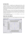
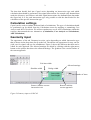
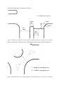
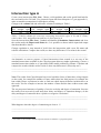
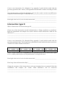
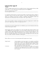
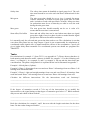
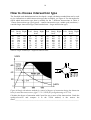
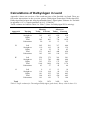
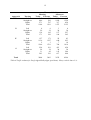
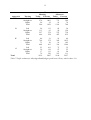
LINKÖPINGS TEKNISKA HÖGSKOLA
ITN/Johan Janson Olstam
TNK062 Traffic modeling
Traffic signals 2007
2007-11-23
Computer exercise
with Capcal
1
Introduction
This computer exercise is an introduction to the calculation program Capcal 3. Capcal
(CAPacity CALculation) is a computer program for calculating effects of intersections and
roundabouts. In this exercise you will practice calculations of non-signal intersection, signal
intersections, and roundabouts. For some of the tasks will blueprints from VU-94 (Road
design 94) be used, these blueprints is available in the appendix (but not in digital form).
Except the guidance in this document there is also a program manual at c:\program\capcal3
(unfortunately only in Swedish) and a help function which can be accessed via the F1-button
on the keyboard.
The aim with this exercise is to increase your knowledge on different intersections types’
effects intersection performance. The aim is also to increase the understanding of how
different traffic signal strategies work and which effect they have on an intersection. The
examination in the traffic signal part in the course TNK062 Traffic modeling will include a
small project with Capcal and the aim of this exercise is therefore also to give basic
knowledge for running Capcal.
In this document will menu and tab choices be written in bold style, for example: perform
calculation (Calculation, Intersection).
Input and calculation
Start Capcal from the shortcut on the start menu and program\Capcal\. Input data to Capcal is
prepared in the tabs Geometry/overview, Volumes, and Signal. There is also a tab for Report
and Printout, see Figure 1.
Figure 1 Screen picture from CAPCAL
2
The data that should feed into Capcal varies depending on intersection type and which
calculation that should be performed. Non-signal intersections for example only demand data
under the Geometry and Volumes tab while signal intersections also demand input data under
the Signal tab. It is for each intersection type only possible to edit the data needed for the
calculation of the specific intersection type.
Calculation settings
Capcal can be used to conduct different kinds of calculations. The type of calculation should
be performed can be edited from the Calculations menu by marking or unmarking Cost
Analysis and ADT-Calculation. We will not conduct any cost or ADT-calculations within this
exercise, thus unmark the two alternatives (Calculations, Cost Analysis and Calculations,
ADT-Calculation)
Geometry input
The appearance of the tab Geometry/overview varies depending on which intersection type
that is chosen in the drop-down list up to the left. The tab has one appearance for stop, one for
yield, one for signal, and one for roundabouts. Figure 2 shows the different data that can be
edited for each approach. The allowed turnings are edited by clicking with the right mouse
button on the picture that shows the allowed turnings. The gradient is the vertical incline of
the current approach.
Exit lane width
Allowed turnings
Shoulder width
Refuge width
Lane width
Lane length
Remove/Add the current
intersection exit
Figure 2 Geometry input to CAPCAL
Number of lanes
Remove/Add the
current approach
3
Some of the input data is illustrated in Figure 3.
Distance to stop line
Angle
Refuge
width
Radius
Exit
width
Lane
width
Figure 3 Illustration of some of the geometric input data (Source: Capcal User manual)
Figure 4 and Figure 5 illustrate some additional geometric input data for roundabouts.
l = length of merging area
b = width of merging area
Figure 4 Illustration of some of the geometric input data (Source: Capcal User manual)
4
The width of the merging area is no longer used in Capcal. Instead the number of circulating
lanes should be specified, i.e. number of lanes in the roundabout and not the number of lanes
in the approaches. The length and the number of lanes in the roundabout are specified under
the Header Roundabout, see screen-shot on next page.
l
Figure 5 Illustration of geometric input data for roundabouts in Capcal
Traffic input
Each approach and turn relation has to be assigned a traffic volume (vehicles/h). The
proportion of trucks in percent is edited in the box besides the truck symbol. The bicycle edit
box refer to the number of bicycles (cycles/h) driving among the vehicles in the lane, thus not
bicycles on separate tracks. The pedestrian edit box refer to pedestrians and bicycles that cross
the approach using an zebra-crossing, but only if the zebra crossing lies in connection with the
intersection.
5
Intersection type A
Create a new intersection (File, New). Choose yield regulation and set the speed limit both for
the road and local to 50 km/h. Use geometric input data from blueprint A-3 gm (appendix 1),
make reasonable assumptions for data that is missing.
Change to the volumes tab and add traffic volumes according to Table 1.
left
A
straight
340
right
120
left
B
straight
right
left
90
C
straight
400
right
left
45
D
Straight right
70
Table 1 Vehicle volumes for exercises concerning intersection types A, B, and C. Heavy
vehicle share 10%, and pedestrian and bicycle flow equal to 0.
Save the intersection (File, Save). Conduct calculations (Calculation, Intersection) and view
the results under the Report and Print tab 1 . It is possible to choose which input and output
data that should be shown.
Change regulation to stop instead of yield. Save the intersection with a new file name and
redo the calculation. Compare the results, are there any differences? If so what is the reason?
___________________________________________________________________________
___________________________________________________________________________
An alternative to start to prepare a Capcal intersection from scratch is to use one of the
standard intersections available in the Capcal program directory under typkorsning. Choose a
standard intersection similar to A-3gm and feed the model with traffic volumes. Calculate and
compare the results with the earlier results. Is there any differences? (Why/why not?)
___________________________________________________________________________
___________________________________________________________________________
Note: The results from Capcal depend on several variables. Some of them have a large impact
on the result, for example the number of lanes while other has little impact, for example the
lane width. Please experiment in order to find out which impact different variables have on
the result. Test for example to increase the number of lanes and the lane width at some other
approach.
The two most used measures of quality-of-service are delay and degree of saturation. Increase
the traffic flow successively and study how delay and degree of saturation changes, do the
delay and degree of saturation have a positive or negative correlation?
___________________________________________________________________________
___________________________________________________________________________
What happens when the degree of saturation gets close to 1?
___________________________________________________________________________
___________________________________________________________________________
1
The results are also saved in the file capout.xls which is available in c:\program\capcal3\.
6
Quality-of-service measurements
The document VU-94 (http://www3.vv.se/vu94s2/) include a quality-of-service measurement
based on the degree of saturation, see Table 2. The measure is defined per lane and refers to
the lane with the highest degree of saturation.
Intersection type
ABCD
E
High standard
<0,5
0,5-0,7
Moderate standard
0,5-0,7
0,3-0,5; 0,7-0,8
Low standard
>0,7
<0,3; >0,8
Table 2 Quality-of-service measure based on degree of saturation according to VU-94.
Grade the level of service for the A-3gm intersection – and henceforth – according to Table 2.
How good is the quality-of-service?______________________________________________
___________________________________________________________________________
Other quality-of-service measures are delay and queue lengths. Delay is probably the measure
that most road users observe. Delay is also the measure that is easiest to express in monetary
terms. Queue lengths are important for dimension of extra lanes in an intersection (vehicle
store possibilities) and for controlling that the queues do not block intersections upstream.
Intersection type B
What is characteristic for intersection type B?______________________________________
___________________________________________________________________________
Create a new intersection (File, New). Use blueprint B-3gm (appendix 1b) feed the model
with the necessary geometric data. Choose yield regulation. Add traffic volumes according to
Table 1.
Save the intersection, conduct the calculation, and view the results. Are there any differences
compared to intersection type A? Why/why not?____________________________________
___________________________________________________________________________
___________________________________________________________________________
How high is the level of service for this intersection?_________________________________
___________________________________________________________________________
Intersection type C
What is characteristic for intersection type C?______________________________________
___________________________________________________________________________
7
Create a new intersection. Use blueprint C-1g (appendix 2) and feed the model with the
necessary geometric data. Choose yield regulation and add traffic volumes according to Table
1.
Save the intersection, conduct the calculation, and view the results. Are there any differences
compared to intersection type A? Why/why not?____________________________________
___________________________________________________________________________
___________________________________________________________________________
How high is the level of service for this intersection?_________________________________
___________________________________________________________________________
Intersection type D
What is characteristic for intersection type D?______________________________________
Choose any of the intersections model calculated above. Change regulation to roundabout.
Redo the calculations and compare the results with the chosen intersection. What are the
differences? _________________________________________________________________
___________________________________________________________________________
___________________________________________________________________________
Create a new intersection. Use blueprint D-4g (appendix 3) and feed the model with the
necessary geometric data. The B-street have speed limit 50 km/h while the other streets have
70 km/h. Use traffic volumes from Table 3.
left
230
A
straight
790
right
160
left
30
B
straight
140
right left
200 330
C
straight
530
right
40
left
230
D
Straight right
190
490
Table 3 Traffic volumes for a roundabout for the afternoon peek. Heavy vehicle share equal
to 10 %, and a pedestrian flow of 230 pedestrians/h crossing the B-street.
How high is the level of service for this intersection?_________________________________
How long is the total interaction delay?____________________________________________
Change the geometry of the intersection to only one incoming lane per approach. Redo the
calculations and compare the results. What differences can be observed?
___________________________________________________________________________
___________________________________________________________________________
8
Intersection type E
Terms
Open the standard intersection Eovra4 (available from the Capcal program directory under
typkorsning). View the signal phases and signal groups from the Signal tab.
How many signal groups are there? ______________________________________________
How many phases are there?____________________________________________________
It is possible to edit the phases as one desire but with the restriction that primary conflicts is
not allowed. There are also some other restrictions. Test to allow straight forward traffic in
phase 2 by clicking on the arrow. Conduct a calculation, what happens? (Notice the
information in the information field at the bottom of the Capcal window)________________
___________________________________________________________________________
___________________________________________________________________________
Thus, it is not possible to conduct a calculation when the phase configuration is conflicts with
the rules for signal groups, which is the signal group rules?____________________________
___________________________________________________________________________
___________________________________________________________________________
Information about which conditions that is not fulfilled is given at the information field at the
bottom of the program window.
Edit the phase pictures to the original set up. Click with right mouse bottom on phase 2 and
click on Edit in the pop-list that appears. It is now possible to edit the phase freely. It is now
possible to allow right turnings from approach D, do so and then close the dialog box. The
phase now becomes grey, which means that there exists a primary conflict. However if it in
this case is possible (enough space etc) to turn left from C and right from D at the same time
there is no conflict. Perform a calculation, what happens? _____________________________
___________________________________________________________________________
Below follows an overview of some important traffic signal terms in Capcal
Signal control
Capcal calculates a fixed time signal, i.e. the signal is not affected
by the traffic in real-time. The signal control should be changed to
Signal group control when modeling modern adaptive traffic
signal. Capcal then performs a correction of the results so that they
better correspond to a modern traffic signal.
Cycle time
The cycle time can be set by the user (30-200s) or be set to be
calculated by the program (40-120s). If Capcal is set to calculate
the best cycle time, all values between 40 and 120 s with intervals
of 5 s is tested.
9
Safety time
The safety time cannot be handled at signal group level. The safe
time must instead be set to the safe time that is dimensional for the
phase.
Min green
The min green time should be set to 4 or 6 seconds for motor
vehicles (normally 4 seconds at roads with speed limit 50 km/h
and 6 seconds at roads with speed limit 70 km/h). Min green time
for pedestrians must be set so that they are able to cross the road
during the min green time.
Max green
The max green time should normally not be set. A value of 0
means that the max time is unrestricted.
Start offset, End offset
Start and end offset time can be used when more than one signal
group have right of way in a phase in order to model that the signal
groups have different start and/or end times.
It is normally only the safe and min green time that needs to set. The calculations is not that
exact that offset times has any large impact. Capcal is not recommended for calculations of
coordinated traffic signals since it cannot handle the effects of the coordination. Capcal will
give a higher delay than reasonable. For coordinated systems one should use programs like
TRANSYT.
Tasks
Do calculations for example 1-3 from TV131 (see appendix 4-7). Please observe that there is
both morning and afternoon traffic volumes available for example 3. Use the following safe
times: 3 s (example 1), 4 s (example 2), and 5 s (example 3). Do not take the short lanes into
considerations. The phase configurations is explained below and in illustrated in appendix 7.
Example 1: Mixed phase (2-phase).
Example 2: Phase 1 all turnings from west and east. Phase 2 all turnings from east. Phase 3 all
turnings from north and south.
Example 3: Phase 1 right and straight turnings from west and east. Phase 2 all turnings from
north and south. Phase 3 left turnings from west and east. Phase 4 all turnings from west.
Calculate the different intersections. Do the intersections work sati factionary?
___________________________________________________________________________
___________________________________________________________________________
___________________________________________________________________________
If the degree of saturation exceeds 0.7 for any of the intersections try to modify the
intersections or the signal timing so that degree of saturation gets below 0.7. Which methods
did you test and which of them worked? __________________________________________
___________________________________________________________________________
___________________________________________________________________________
Redo the calculations for example 1 and 2 but now with the length restrictions for the short
lanes. Do the results change noticeable? ___________________________________________
___________________________________________________________________________
10
How to choose intersection type
The Swedish road administration has developed a rough calculation method that can be used
to give indications on which intersection type that is suitable, see Figure 6. Use the method to
check which intersection type that is suitable for the 7 different intersections in Table 4.
´Choose Intersection type (god (good) = smaller intersection type, mindre god (moderate) =
consider larger intersection type, black marked area = larger intersection type).
Left
90
90
90
90
90
130
230
A
Straig Right
ht on
340
120
340
120
340
120
230
120
90
60
90
60
550
120
Left
70
150
40
75
75
130
70
B
Straig Right
ht on
65
40
65
40
65
150
65
40
65
40
65
40
65
40
Left
90
90
90
90
90
90
115
C
Straig Right
ht on
400
95
400
95
400
95
220
95
150
95
150
95
650
120
Left
45
150
70
65
65
65
45
D
Straig Right
ht on
30
70
30
70
30
150
30
70
30
70
30
70
30
70
Table 4 Traffic volumes for 7 different intersections.
Figure 6 Rough calculation method for control of degree of saturation during the dimension
hour for an urban intersection. (figur 7.5.2-2, VR50 för fyrvägskorsning ur VU-94)
Calculate the degree of saturation with Capcal for one or more of the intersections. Grade the
quality-of-service and compare it to the VU94 method, is the answer the
same?______________________________________________________________________
11
Calculations of Dalbyvägen in Lund
Appendix 8 shows an overview of the south-east parts of the Swedish city Lund. There are
four main intersections in the overview picture (Dalbyvägen/Tornavägen, Dalbyvägen/E22,
Dalbyvägen/Porfyrvägen and Albyvägen/Sandbyvägen). Signal phase schemes are available
in appendix 9-12, i.e. signal controllers 46, 912, 15 and 941.
Traffic volumes are found in Table 5 to Table 7 (flows for Dalbyvägen/E22 is missing).
Flow (vehicles/h)
Morning
Afternoon
Today
Forecast
Today
Forecast
34
49
52
73
303
423
656
918
8
11
28
39
345
483
736
1030
20
30
13
15
Approach
W
Turning
Left
Straight on
Right
Total
Pedestrians
N
Left
Straight on
Right
Total
Pedestrians
205
110
18
333
143
281
162
22
465
189
317
99
32
448
196
444
139
45
628
223
E
Left
Straight on
Right
Total
Pedestrians
258
513
393
1164
43
372
748
578
1698
57
201
460
175
836
45
281
644
245
1170
60
S
Left
Straight on
Right
Total
Pedestrians
9
118
181
308
101
13
164
255
432
129
13
99
318
430
73
18
139
445
602
100
2150
3078
2450
3430
Total
Table 5 Traffic volumes for Tornavägen/Dalbyvägen (peek hour). Heavy vehicle share 3 %.
12
Flow (vehicles/h)
Morning
Afternoon
Today
Forecast
Today
Forecast
167
225
102
147
446
599
1054
1520
571
767
317
458
1184
1591
1473
2125
Approach
W
Turning
Left
Straight on
Right
Total
N
Left
Straight on
Right
Total
4
29
138
171
6
39
185
230
3
24
157
184
4
34
227
265
E
Left
Straight on
Right
Total
127
1136
2
1266
171
1527
3
1701
58
640
7
704
83
923
10
1016
S
Left
Straight on
Right
Total
224
28
31
283
301
38
42
381
451
24
143
617
650
34
206
890
2904
3903
2978
4296
Total
Table 6 Traffic volumes for Porfyrvägen/Dalbyvägen (peek hour). Heavy vehicle share 3 %.
13
Flow (vehicles/h)
Morning
Afternoon
Today
Forecast
Today
Forecast
180
647
467
252
276
1001
733
386
50
22
18
70
506
1670
1218
708
Approach
W
Turning
Left
Straight on
Right
Total
N
Left
Straight on
Right
Total
26
113
527
666
113
63
378
554
82
50
275
407
36
158
738
932
E
Left
Straight on
Right
Total
46
769
73
888
21
372
20
413
18
282
14
314
69
1035
102
1206
S
Left
Straight on
Right
Total
23
39
17
79
2139
101
136
113
350
2987
73
97
81
251
2190
32
55
24
111
2957
Total
Table 7 Traffic volumes for Albyvägen/Sandbyvägen (peek hour). Heavy vehicle share 3 %.