1
ITN/LINKÖPINGS TEKNISKA HÖGSKOLA
Johan Janson Olstam & Andreas Tapani
TNK082
1/28/08
Computer exercise 2
Simulation in AIMSUN/2
Computer exercise 2 – Description
The computer exercise is an introduction to how to conduct simulations using AIMSUN/2. In this
computer exercise the networks which were created in computer exercise 1 will be simulated and
analyzed. The aim of the exercise is to give basic knowledge on which settings that should or could be
changed, which statistics that can be gathered, how to choose and interpret output data, etc.
This exercise consists of 3 obligatory tasks. The first task is to simulate the three obligatory networks
from computer exercise 1 and answer questions about traffic flow levels, average speeds, etc. The
second task is to run several replications in order to study how well one replication represents the
more representative average from several replications. The third and last task is to test different route
choice models and analyze how different models affect the result from the simulation.
Menu and tab choices will in this document be marked using bold font, e.g. save the network (File,
Save as). Selection or marking of radio buttons or check boxes or writing values in edit boxes will be
marked with italic font, e.g. set the lane width to 3.5 meters by writing 3.5 in Lane Width.
Examination
You have to solve task 1-3 in order to pass the exercise. Present your solutions to the supervisor at the
end of the scheduled class.
Settings in AIMSUN/2
Start by open up the AIMSUN program, there is a short-cut on the start-menu under
program\GETRAM v4.2.
Load the network
In order to simulate a network, the network and corresponding Result Container OR OD-matrix has to
be loaded into AIMSUN. Also public transport plans and signal controls, if any, has to be loaded.
Following is a description on how to load these different modules:
•
Load the network: File, Load Network and then locate your network in the Directory drop-down
list.
•
Load turn proportions (Result container): File, Load Traffic Result and choose the created
Container. Mark the created state under States. Choose exponential arrivals.
•
Load the OD-matrix: File, Load O/D Matrix and choose the created OD-matrix. Choose
exponential arrivals.
•
Load the public transport plan: File, Load Public Transport.
•
Load the traffic signal control, File, Load Control.
It is possible to save a certain combination of network, OD-matrix, signal control, etc in a scenario
(File, Save Scenario). Next time you want to open this setup is it sufficient to open the scenario (File,
Load Scenario).
Statistics settings
The results from a simulation in AIMSUN/2 can be illustrated in several ways. It is possible to create
reports directly in AIMSUN (Reports, Current Report, Statistics). It is also possible to save the
output data in a text-file or in a database, which is preferable. If data is to be stored in a database, copy
the file ”getram_42.mdb” from s:\TN\K\TNK082\Lab 2 to a suitable folder on your home directory.
To save the output data in a text file or in a database do the following:
Page 2 (7)
•
Text file: Experiment, Output, Output Location and choose To ASCII Files and a suitable
directory.
•
Access database: Experiment, Output, Output Location and choose To Access Database and
the copy of "getram_42.mdb".
Now it is time to choose which statistics that should be collected and calculated (Experiment,
Output, Statistics). Choose for example the following
•
Gather Statistics.
•
Periodic, set the Time interval to 30 minutes.
•
Store output.
•
System, Sections and Vehicle Types under the General tab.
•
All and Turns under the Sections tab.
Simulation settings
The simulation should be run for the time period 700 - 900 (Experiment, Run Time). Set Simulated
Initial Time to 07.00 and Simulated End Time to 09.00. Set Warm-up period to 30 minutes.
There are also settings concerning the animation of the vehicles. The vehicles can for example be
given different colors depending on their destination (Only possible when using an OD-matrix). In
order to do that the different centroids have to be given different colors. Open View, Preferences and
choose Centroid under Colors in the tree structure. Click in the Enable column for all centroids. Then
double click in the Color field and choose color by adjusting the color-bars. To color the vehicles by
destination choose View, Vehicle Colouring, Destination. It is also possible to color the vehicles by
their next turning, vehicle type, etc.
Before running the simulation some settings regarding the driver behavior have to be changed. Open
(Experiment, Modelling) and change the following settings:
•
•
•
Under the General tab:
○
Simulation Step = 0.75 s
○
Reaction Time at stop = 1.00 s
○
Queuing Up Speed = 1.0 m/s
○
Queue Leaving Speed = 4.0 m/s.
Under the Car Following tab:
○
Car Following Model: 4.2
○
Apply 2 lanes Car Following model (mark)
○
Number of Vehicles = 4
○
Max distance = 100.0 m
○
Max Speed Difference = 50 km/h
○
Max Speed Difference On Ramp = 70 km/h.
Under the Lane Changing tab:
○
Percent Overtake = 0.900
○
Percent Recover = 0.950
○
On Ramp Model: 3.3.
Page 3 (7)
In order to be comparable, the simulations of the different networks should be run with the same initial
values in the random number generator. Set the Random Seed number to 3871 in the dialog box
(Experiment, Replications).
Simulation
The simulation can be controlled either via the Run menu or via the media player buttons at the bottom
of the window. There are several different run options:
•
Run, simulation with animation. The simulation speed can be controlled using the bar on the
right-hand side of the record button.
•
Step, stepwise simulation, one simulation step per button click.
•
Batch, simulation without animation.
The simulation can be stopped using (Run, Stop). The simulation can be started again using any of the
run alternatives. To restart the simulation from the initial start time the simulation has to be reset by
pressing the rewind button or (Run, Begin).
Results
After a completed simulation, the results can be viewed by opening one of the output text files or the
database file. It is recommended to save the data in a database file. This makes it easier to view limited
parts of the data and to copy it to other calculation programs as Excel or Matlab.
The database file includes several tables. The following tables are of most interest during this exercise:
•
SectSta, includes information on flows, travel times, etc. for the different sections.
•
SysSta, includes flows, travel times, etc. for the whole network.
•
TurnSta, includes flows, turn times, etc, for all turnings.
In the output text-files the turn statistics is presented in connection with the section statistics.
Some of the columns in the database tables are sometimes difficult to interpret. The following is a
explanation of some of the columns.
•
tfrom, is the start time of the statistics period in seconds, 700 is equal to 25200 seconds after 000.
•
tto, is the stop time of the statistics period in seconds, 730 is equal to 27000 seconds after 000.
•
flow, is the traffic flow in vehicles/hour.
•
hspd1, is the harmonic mean speed in km/h. The harmonic mean speed (also known as the space
mean speed) for a section is the travel mean speed.
•
hspd2, is the deviation of the space mean speed.
•
ttime1, is the travel time in seconds.
The definition of the different tables and columns can be found in Appendix 2 in the AIMSUN v4.2
User Manual. The manual is available under s:\GETRAM manualer\.
Page 4 (7)
Task 1 – Simulation of network 1, 2 and 3
Conduct simulations of the networks corresponding to task 1-3 in computer exercise 1. Remember to
save the results in different database files. Answer the questions below using statistics from the second
half hour period, i.e. 730 - 800.
Network 1 – Turn proportions
1. How large is the traffic flow, the average travel time, and the average speed on the following
sections?
Section
Flow
Travel time (s)
Speed (km/h)
4
10
11
12
2. How large is the total flow in the system?
Answer:__________________ vehicles/h
3. How long is the average travel time in the system?
Answer:__________________ seconds
4. How high is the average speed in the system?
Answer:__________________ km/h
5. How many vehicles turns left from section 10?
Answer:__________________ vehicles
Network 2 – OD-matrix
1. How large is the traffic flow, the average travel time, and the average speed on the following
sections?
Section
Flow
Travel time (s)
4
10
11
12
2. How large is the total flow in the system?
Answer:__________________ vehicles/h
3. How long is the average travel time in the system?
Answer:__________________ seconds
4. How high is the average speed in the system?
Answer:__________________ km/h
5. How many vehicles turns left from section 10?
Answer:__________________ vehicles
Page 5 (7)
Speed (km/h)
Network 3 – Traffic signals
1. How large is the traffic flow, the average travel time, and the average speed on the following
sections?
Section
Flow
Travel time (s)
Speed (km/h)
4
10
11
12
2. How large is the total flow in the system?
Answer:__________________ vehicles/h
3. How long is the average travel time in the system?
Answer:__________________ seconds
4. How high is the average speed in the system?
Answer:__________________ km/h
5. How many vehicles turns left from section 10?
Answer:__________________ vehicles
Comparison of the networks
1. Are the results for Network 1 and Network 2 equal? Why/Why not? Should they be equal?
Answer:_______________________________________________________________________
_______________________________________________________________________________
_______________________________________________________________________________
_______________________________________________________________________________
_______________________________________________________________________________
_______________________________________________________________________________
2. How does the introduction of traffic signals affect the performance of the Network?
Answer:_______________________________________________________________________
_______________________________________________________________________________
_______________________________________________________________________________
_______________________________________________________________________________
_______________________________________________________________________________
Page 6 (7)
Task 2 – Several replications
Load Network 3. Choose to run replications (Experiment, Replications), mark multiple and write 10
in Number of replications and press the Create button. How many replications that are needed when
conducting a simulation depend on the desired significance level. You can read more about how to
calculate the needed number of replications in the AIMSUN manual in chapter 7.4.1 Calculation of
the number of replications at page 166. Press Simulate in order to start the simulation. Note! All
replications are run in batch-mode.
1. Compare the average values from the 10 replications with the results from the replication with
Seed 3871. Do the results from the 3871 replication deviate much from the average from the 10
replications?
Answer:_______________________________________________________________________
_______________________________________________________________________________
_______________________________________________________________________________
_______________________________________________________________________________
Task 3 – Route choice
All simulations so far have been conducted assuming that all vehicles choose the shortest route
between the origin and the destination. AIMSUN offers several options and models for vehicles route
choices. The route choices can either be modelled as a fixed or a dynamic choice. Load Network 3.
Change the route choice to fixed (time) instead of fixed (distance) in (Experiment, Route Choice).
Run the simulation.
1. Did the vehicles route choices change? (Hint: check the turn statistics, for example for left turners
from section 10.)
Answer:_______________________________________________________________________
_______________________________________________________________________________
_______________________________________________________________________________
_______________________________________________________________________________
Now change the route choice model to a Multinomial Logit model. Let the cycle time be 5 minutes, i.e.
the shortest paths will be updated every fifth minute. Let the number of intervals be 1 and set the
capacity weight to 1, the higher value the higher “punishment” for paths with low theoretical capacity.
Choose Yes in the Dynamic drop-down list. Set Initial K-Sps to 1 and Max number to keep to 5. Set
Max number of Route to 3. Finally set the parameter θ in the logit model, to 10. Each vehicle will now
choose their route according to the path they observe as the best when they enter the network.
2. Did the vehicles route choices change?
Answer:_______________________________________________________________________
_______________________________________________________________________________
_______________________________________________________________________________
_______________________________________________________________________________
_______________________________________________________________________________
3. Do the route choices vary over time?
Answer:_______________________________________________________________________
_______________________________________________________________________________
_______________________________________________________________________________
_______________________________________________________________________________
_______________________________________________________________________________
Page 7 (7)