1
Engineering 164 Lab Manual
Spring 2001
Laboratory Exercise 3: A DSP-Based Interference Filter
and Automatic Gain Control System
It is now about seventeen years since the compact disk, developed by Phillips Laboratories in Briarcliff Manor, New York, began to change the way we listen to music and to
improve the quality of recorded music tremendously. Digital technology will eventually
pervade the entire home music system. All sources will be digital and the digital data
will be manipulated to do tone compensation and room equalization before the data is fed
to a DAC and power amplifier. Even the radio receiver will come to depend on digital
filtering techniques to lower cost and improve performance. The basic method for this
filtering is one of the concepts behind this lab. While I am not trying to teach the
mathematics of digital filtering, I do hope you pay attention to the mechanics of the process and come to understand some of what one can do in this field.
I also have a continuing interest in another area of new product development, even
though I do not work in it. I have a nephew who is profoundly hearing impaired, for
whom hearing aids have been a great help and a continuous hassle. Such aids are still
largely analog designs, but Siemens and other companies have begun offering digital
ones. The basic function of a hearing aid is to filter the microphone signal to match the
limited range of frequency response – typically a band only a kilohertz or so wide around
1KHz – of a particular deaf person. (Ideally this response should be tailored to the person for the greatest effectiveness and the least damage from acoustic overload.) Hearing
aids also need to adjust their gain to match the level of signal in the room because the
main problem in deafness is the lack of dynamic range. You have to boost any signal,
weak or strong, to a fairly loud but not damaging level. You have to do so in a way that
does not distort the signal when the room noise level increases. This change of gain has
to occur on a fractional second basis with no intervention of the user. Analog hearing
aids use an Automatic Gain Control circuit for this function. Again in the context of presenting the instruction set and capabilities of a DSP processor, we have designed an AGC
algorithm into the lab that does the same thing digitally.
The two capabilities of the program – filtering and AGC – are applicable to both music
systems and hearing aids. In audio systems, the equivalent of AGC is found in the Dolby
compression system that allows limited dynamic range media, such as analog cassette
tapes and movie sound tracks, to seem to have more range. The trick is to crank up the
gain in recording when the signal is weak and crank the gain down again when the signal
is strong. You do the reverse in playback. Your DSP program is equivalent to the recording end of this process. You can probably figure out an inverse algorithm for playback.
The Analog Devices Corporation has graciously donated six SHARC evaluation boards
with ADSP21061 processors as the basis for the lab. Each board also has a two-channel
codec chip that contains both analog to digital and digital to analog converters. (These
codecs are the basis for SoundBlaster cards and similar motherboard capabilities in
PCs. The two channels are the left and right stereo signals. You only have to deal with
34
Engineering 164 Lab Manual
Spring 2001
one of them.) The gift package included a program for taking data from the ADC’s and
putting it back out to the DAC’s. I have modified that program to store blocks of data on
the way through. This allows you to manipulate the data with an assembly language program. To do the entire job requires about 80 lines of code. This is not easy code to write
– you can make very subtle mistakes. I have tried to tell you how to avoid problems, but
you should build and test the code section by section, and you may need to test your work
with the simulator. I hope to offer a shell program for exercising your code in the simulator without your having to worry about setting up input data or simulating the DMA
input and output transfers.
Requirements: Write an assembly language program for an Analog Devices SHARC
processor to do notch filtering and/or AGC on a digital signal stream. There are two
switches on the board that your program will read to determine whether data is filtered,
AGC’d, both or neither. There is a block diagram of the system at the beginning of the
discussion section. The system has been set up and completely wired on Analog Devices
boards. You provide and integrate the actual processing code.
You can receive 65 % of the grade for the lab by getting the data transfer and digital filter
parts to work properly. (These operations take 90 % of the computation time, but the
AGC is the hardest part to write.) It is easier to show than to explain the simple procedures we have for testing the system. For this reason, the details on testing the code are a
bit vague and will have to be explained more during the lab and help sessions.
We have placed copies of a template for an assembly-language subroutine called
“Lab3_00.asm” both on the class website and on the Instructional Computing Facility
machines. (See the discussion section for access details.) Make a copy of that file using
your own unique file name but with the same “.asm” extension. There is also source
code and object code for a mixed C and assembler program that I wrote by modifying the
Analog Devices “TalkThru” program. You are welcome to look at the source code, but
its details are of little real interest. (I am not particularly proud of it – it is really very inefficient! Still it does the job and could be written and debugged quickly.) When the
“Lab3_00.asm” routine is properly assembled and linked with my code, it is called periodically whenever there are 512 new data points available to process. Those data are 32bit fixed-point integers whose magnitudes are always less than 32768. (They start as 16bit two’s complement numbers from the codec and are sign extended to 32 bits.) You
must write SHARC assembler code to do the filtering and AGC control on this data and
write it back to an output buffer for the calling program to send to the codec.
The template file has clearly marked places for allocating space for variables and buffers
in both program and data memory as well a place for your code. There is a header section with definitions for SHARC parameters and for some constants used in the algorithms. Finally, the code section has a short piece of program that I originally used to
check that the template worked. It copies the fixed-point input data directly to the output
buffer. This code is now commented out, and you should remove it altogether before
turning in your code. I left it in place so you would have a simple guide to common syntax and could use it as an example of retrieving and returning the signal data.
35
Engineering 164 Lab Manual
Spring 2001
When your subroutine is called, the address of the start of the input data array, effectively
a pointer to the array, is stored in data memory at the location “_InAddress”. (The leading underscore is necessary!) You can retrieve that pointer to a register, say to register i1,
with the expression “i1 = dm(_InAddress);”. Similarly the memory location
“_OutAddress” has the address of where to place your output data. Do not modify these
pointers! Your code must do the following:
1. Retrieve 512 integer inputs from the array at “_InAddress”, convert them to
floating point numbers, and store them contiguously to the last set of data in a
buffer of your own. (Floating-point conversion is necessary because both the
processing algorithms use floating-point numbers.) Very likely you would use a
circular buffer to make building the filtering algorithm easier. (The discussion
section talks about these buffers as does the material on DAG’s in the software
handout.)
2. Filter all the data from the new frame. I have provided a set of filter coefficients,
that is, a set of constants, in program memory. The number of such coefficients is
given in a #define statement at the top of the code as NCOEFFS. Suppose that
the data in your floating-point buffer are called { f i } where i is an index corresponding to sample number. (This index simply increases continuously with
time. Since there is only a finite amount of memory, the buffer locations are cyclic and i amounts to an index through the buffer.) The filtering formula is:
xi =
NCOEFFS −1
∑c
j =0
j
⋅ f i− j
where cj is the jth coefficient and xi is the ith output of the filter. On subroutine
entry, the values of these coefficients are found in program memory as an array
starting at address “_coefs”. Each filter output is affected only by the current input and by the last NCOEFFS – 1 inputs. Thus you will save two frames of input
data, replacing the oldest with a new set on each frame. The old data you have
left are needed to calculate the first outputs of the new frame. You will have to
store the new outputs {xi} in a separate working storage area.
3. There is an integer in the range 0 ≤ n ≤ 3 passed to you in the memory location
“_InFlags”. If this number is 2 or 3, apply AGC to the {xi} values that you just
calculated. The AGC algorithm is discussed more below.
4. After you have finished the calculations, convert the {xi} values to fixed-point
numbers and write those out to the output buffer at “_OutAddress”.
The digital filter is primarily a notch filter, that is, it removes a portion of the frequency
spectrum between 4 and 4.5 Kilohertz. (By remove, we mean that it reduces the magnitude of a sinusoid in this frequency range by a factor of 1000 or so.) To test your filtering
code, we will have signal sources that mix a pure tone in this band with a normal source
like a tape or CD player. Without filtering, the pure tone masks much of the music. With
filtering, the tone disappears, but there is little effect on the rest of the signal.
36
Engineering 164 Lab Manual
Spring 2001
The AGC algorithm itself is slightly complicated, but the required code is not long (46
lines). You will need to do an inverse square root operation, for which the code may be
taken verbatim from the Analog Devices user’s manual. (The algorithm uses the Newton-Raphson iterative method with an initial guess supplied by the RECIPS assembler
instruction. Remember the homework? The description of the syntax of that instruction
contains code for the full calculation.) I have made life a little easier by typing the code
from the manual into the “Lab3_00.asm” template file as a subroutine at the end of the
file. You will need to consult the Users’ Manual to figure out how to use the code. The
idea of the AGC algorithm is to estimate the average amplitude of the incoming signal. If
this is small, then multiply each signal point by a large gain. Similarly if the amplitude is
large, multiply by a smaller gain. You can do this easily by making the gain inversely
proportional to the average amplitude. To avoid an infinite gain when the signal disappears, one adds an extra constant into the denominator to keep it non-zero. In the algorithm below, the first two steps calculate the mean square amplitude. The third step calculates a new gain, which is applied to the data in the fourth step. After compensation for
overload from abrupt increases in the input, the data is converted to integer format and
stored. The exact algorithm is:
For each new frame of 512 data points, let xi be the ith output of the FIR filter where in
this case 0 ≤ i ≤ 511 . Let si be the DAC output signal for this sample. Let Y be a running measure of the energy in the signal which we recalculate for each frame with the
511
expression Ynew = A ⋅ Yold + ∑ xi2 where A is a constant with value 0.982. This will give
i =0
an average value of the square of the signal amplitude over roughly a second. From this,
C
we calculate a new gain Gnew =
and each si = Gnew ⋅ xi . Step by step, the algoB + Ynew
rithm is:
511
1. X = ∑ xi2
i =0
2. Y = A ⋅ Y + X
3. G =
C
B +Y
4. for (i=0; i < 512; i++) {
s i = G ⋅ xi
if |si | > SMAX then
{
si = CLIP si BY r0; where r0 contains SMAX.
Y = D ⋅ xi2 − B
37
Engineering 164 Lab Manual
G=
Spring 2001
C
B +Y
}
Store si in either the working buffer or the output buffer. If you write to
the output buffer, then this is where you do conversion from float back to
integer.
}
5. If not already done, store results to the output buffer, converting to fixed-point
integers en route.
6. Store the value of Y in memory for use in the next frame.
The constants A, B, C, D, and SMAX have values A = 0.988, B = 9.77⋅1010, C =
3.127⋅106, D = 1.2⋅104, and SMAX = 28300.0. These values are already entered in “#define” statements at the top of the template file as A_agc, B_agc, etc. The reason to separate steps 1 and 2 is to improve the accuracy of calculating Y – the small terms in x2 will
accumulate more accurately in an empty register than in one filled with a very large
number beforehand.. The “CLIP” operation replaces si with either +28300 or –28300 depending on the sign of si if the initial magnitude exceeds 28300. The format of the CLIP
statement is the syntax of the actual assembler instruction where si is understood to mean
the register in which si is stored. When G is recalculated after the CLIP statement, the
new gain applies only to the later outputs in the current frame. With this choice of constants, the gain for low amplitude signals is 20 DB and the maximum signal to the DAC
is +/- 28300 out of a possible +/- 32767.
The Analog Devices “TalkThru” program that is the basis of my code allows you to
change the analog gain of the codec with a software button on the PC you use to download the program. (Downloading instructions are posted in the lab.) We will test the
AGC control by looking at how your output changes when the codec gain changes. If the
AGC is working, then a 20 DB change in input should produce a 3 to 6 DB change in
output.
When the lab TA certifies that your program works to the level you claim, he or she may
ask some questions about how you designed it. Then to finish getting credit for the lab,
you email the source code to the recording account. Please indicate in the cover message whether both parts (or neither) of the lab work, that is, both filtering and AGC.
Discussion: Figure 12 shows a block diagram of the finished system. The central part of
the drawing is the EZ-Kit LITE evaluation board from Analog Devices. On the left there
is a tape player or CD system, the output of which has a sine wave at a little above 4 Kilohertz added to it. This sinusoid is the interference that your filter must remove. The
combined signal goes to the codec on the evaluation board. There the signal is sampled,
that is, measured repeatedly at a constant rate of 44.1 Kilosamples per second. (The program you use to download the code actually lets you choose the sampling rate from a
Windows menu. You will find that the frequency of the filter notch is proportional to this
38
Engineering 164 Lab Manual
Spring 2001
rate. Use the 44.1 KHz sampling rate for testing. I designed around that frequency because it is the standard for audio data. You should play around to see the effects of
changes.)
Flag Switches
(Inputs)
4.2 KHz
Sinewave
Audio Source
(Tape or CD)
∑
Codec
ADC
FLAG3
Output for Timing
SHARC Processor
Running:
Codec
DAC
Your Subroutine
Powered
Speaker
ICE or In-Circuit Emulator
Test Setup
Analog Devices Evaluation Board
EZ-KIT LITE
Figure 12: Block diagram of the SHARC system for Lab 3
The codec data stream goes to the SHARC processor where my program separates one
channel of data, stores 512 words in memory for you, and calls your program. You process the data and write it back to an output buffer that I send on to the DAC. You can listen to the results on a speaker. There are several other inputs and outputs to the processor. I do not yet know how useful it is in this lab, but we have an In-Circuit Emulator or
ICE available that lets you control running the code and lets you examine memory. (You
can also stop the program and read memory back from the board with the PC. See the
EZ-Kit Reference Manual chapter 3.) We will have at least one station set up with the
ICE, but I may not have had time to figure out exactly how best to use it. Again, feel free
to experiment; the instructions and software will be available. Finally, there are four
“FLAGn” pins on the processor that allow you to put in bits or take them out by hardware. FLAG0 is dedicated to the codec. We have set up FLAG3 as an output pin with a
jack to connect it to a scope or logic analyzer. This pin goes HIGH when your code is
called and goes LOW when it returns. The HIGH time measures how efficient your code
is. (If your code isn’t fast enough, this test will show it – the effect on the audio stream is
pretty clear as well, but this test allows you to separate causes more easily.)
Flags 1 and 2 are input pins connected to switches mounted to the EZ-Kit. We read those
switches before each call to your code and pass the result – a number between 0 and 3 – u
in the memory location “_InFlags”. You use this for controlling whether filtering and/or
AGC is done. This requirement makes it easier to test. (I suggest you apply the filter
only if _InFlags contains 1 or 3. You already apply AGC only if the number is 2 or 3.)
39
Engineering 164 Lab Manual
Spring 2001
This is not a course on digital signal processing, so I give you the algorithms and the constants you need to do the job. However, if you are curious about why the whole thing
works, I recommend the book Digital Signal Processing by Richard Hamming. This is a
skinny, well-written book on the basic ideas of digital filters that I found to be a nice introduction. I will make sure a copy is on reserve in the Sciences Library.
There is an enormous amount of documentation on the SHARC processor and the EZ-Kit
evaluation board. We have put this on the class website and on the Engineering server.
You are welcome to read and copy the material including the programs as much as you
like. The software for the assembler and simulator is a product of the Free Software
Foundation, which encourages its distribution. (This software is not Analog Devices’
latest and greatest. Their newer software concentrates on automating DSP design within
Microsoft’s Studio environment, and it hides the processor properties from the user. The
older software is quite serviceable for my pedagogical purposes, but you should not hold
its clunkiness against the Company.) However, please do not print out big chunks of
stuff. That wastes paper and does you little good. To make it a little easier to write a
program, I have prepared a handout that contains selected material taken from the
SHARC reference manual. (Appendices A and B in that manual have the complete description of the instruction set.) The handout contains the chapter on the use of the
DAG's, the Data Address Generators. It also has the index of the instruction set and specific data on a few difficult to understand but very useful instructions. In writing a program, the reference manual is probably the most useful single piece of documentation.
To access all the documentation and source files in The Instructional Computing Lab,
you first have to set up your account. There is a program group called "SHARC EZ-KIT
Lite" in the START menu of the The Instructional Computing Lab machines. First run
the command file called "Environment Setup" in this group by double clicking on it.
This edits your PATH, environment variables, and registry entries to include all the programs necessary to compile, link, and run your code.
The same program group also contains two applications. One is called "EZ-KIT Lite
Host"; this is the program you run to test your code. When you think you are ready to
test your code, launch this application, and select the file created by the assembler. (Even
though you can’t run your code in the Instructional Computing Lab because we don’t
have SHARCs on the machines, the NT machines in room 196 will access both the server
software and an evaluation board.) The other application is the "EZ-KIT Lite Simulator";
use this program to simulate your code if you are having problems.
There is also a link to the folder containing the source files you will use for the lab. The
shortcut is called "EN164 Source Code" and it contains the "Lab3_00.asm" template file
that you will rename and edit. You should copy the contents of this directory to your account and edit code there. (Open Windows Explorer, go to your root directory, and drag
the source folder to your directory.) In the same directory there is a batch file called
“Mk.bat”. Open this with Notepad and edit the end of the first line, changing
“Lab3_wrp.asm” to the name of your file for this lab. When you have entered the code,
40
Engineering 164 Lab Manual
Spring 2001
you can assemble and link the program by double clicking on this file. The executable is
given the name “tt.21k.” You download this file with the “EZ-Kit Lite Host” program.
We have also written a C program that can be used with the simulator to exercise your
code. The same “Mk.bat” file links your code to that program as well, giving the file
“Lab3_sim.21k”. You can run the "EZ-KIT Lite Simulator." on that executable. The
simulator program will let you pick a set of input data, look at the output buffer, and examine how your code works line-by-line. The simulator is similar in operation to the one
for the PIC16C505. It is a little slow but should be fine for your purposes.
In addition, there are shortcuts in the "EN164 Source Code" program group to folders
containing example files and source code, including information about the Analog Devices’ “Talk-Thru” program referenced in this handout. The “TalkThru” program relies
heavily on assembly-language library routines. They are stored in the “Assembly Routines” folder within the EN164 program group. The “EZSharc” folder in the same group
has source code for several applications mentioned in the EZ-Kit reference manual. Each
application is in its own folder, and the “TalkThru” program is in the “tt” folder. You will
not find these programs of much use directly, but you may want to look at them as examples of correct syntax.
In the interests of making your work more efficient and less painful, here are four observations about SHARC programming that represent mistakes I have made at one time or
another. Consider them warnings about the subtle errors one can make on this processor.
First of all, the general register set has only 16 actual registers. These may be referred to
as r0 to r16 or f0 to f16. In the first case, the assembler assumes you mean integer data
and in the second you mean floating point data. There are NO DEDICATED
FLOATING POINT REGISTERS! Be careful that you don’t overwrite data you need by
using a given register under two different names, e.g., f1 and r1.
Second, most compute instructions allow you to fetch or store two pieces of data at the
same time by accessing both program and data memory. By a peculiarity of the assembler, the order of program and data access is important. For example, the line: “r0 = r1 +
r3, dm(i1, m6) = r4, r3 = pm(i9, m15);” is perfectly legal. It adds the contents of r1 and
r3 into r0, fetches a word from program memory to r3, and writes one from r4 into data
memory all in the same clock cycle. The line “r0 = r1 + r3, r3 = pm(i9, m15), dm(i1,m6)
= r4;” is illegal. Note that in dual access with computation commands, the only method
of access is through the use of the DAGs. (There are not enough instruction bits to encode anything more complicated.)
Third, lines that do multiple-operations are subject to some subtle errors the assembler
will not catch, partly because the assembler is no too smart and partly because the operations are not actually illegal. For example, the line: “r3 = r1 + r3, dm(i1, m6) = r4, r3 =
pm(i9, m15);” is perfectly legal but will malfunction. The problem is that there are two
writes to r3 in the same line. The hardware has rules about precedence, and only the
ALU write will actually work. The other is lost. Finally, the digital filtering can be done
in very little more than one instruction per filter coefficient if you use the multifunction
41
Engineering 164 Lab Manual
Spring 2001
instruction that allows you to do a sum and a multiply at the same time as dual memory
reads. I have included the description of this “Parallel Multiplier and ALU (Floating
Point)” instruction in the handout on the instruction set. There are two problems using
this instruction. One is that you have to plan the register use very carefully since it has
severe restrictions on the source registers. The other is that all operations on the line are
done simultaneously. This means the product being accumulated in a step is not the one
being calculated in that step but is the one calculated in the previous instruction. To start
the system up, takes a little thought so that the first sum will add the first product to an
empty register. Because the filtering loop is the most computationally intensive part of
the whole code, using this instruction can make the code much more efficient. In fact, at
the moment, the code will only work if you use this instruction successfully. (We are
working on relieving the constraint but don’t count on our success.)
Finally, a few words about how the DSP instruction set makes signal-processing code
more efficient. My example is the use of circular buffer for your filtering operation. Notice that in the expression for the output of the filter code, xi =
NCOEFFS −1
∑c
j =0
j
⋅ f i − j , the input
data { f i } is indexed backwards, that is, the current output xi depends on not only the current input value fi but also on many earlier samples because the subscript is i-j. Since
memory is a finite resource, you cannot keep putting data into new locations. Instead one
keeps only two frames of data, the one you are working on and the immediately preceding one. Figure 13 shows a circular buffer for this purpose. In the figure, the data for the
current frame has been put in the left half, and the program is processing an output word
corresponding to an input partway through that section. The gray areas show the earlier
data that contributes to the new output. You set up a circular buffer by loading b1 and l1
with the base address and the buffer length. If you then use only the dm(i1, m..) method
of addressing, the processor makes the data addresses wrap around. Thus you can index
backwards through the data with dm(i1, m7) and know that you will bring back data from
the high end of the buffer when you need it. (The m7 register always holds the value –1,
and you must not change that. It is used for stack management in my code.) After calculating the output for one point, you can set i1 to point to the next input point using the
instruction “modify(i1, m1);”. (Of course you load m1 with what you need to add to i1
before you start the calculation. Usually this value is one to three greater than the number of coefficients, being one more than the number of times you decrement i1 during the
calculation.) On the next frame, you put the new data into the right half of the buffer, and
the present data becomes the immediate past data. Keeping track of which half of the
buffer to use in each frame is the main nuisance in the input part of the code. Remember
that you have to set l1 = 0 before leaving your code and, therefore, have to set up the
buffer each time you use it.
42
Engineering 164 Lab Manual
Spring 2001
Base Address
in register b1
New data
Newest data
Oldest data
Recent Data
Calculating for output at this input data point
Length = 1024 words – l1 = 1024;
Figure 13: Memory use for a two-frame, circular buffer. Memory addresses increase to the right.
Each half holds one 512-word frame, and the left side was the most recently filled. The gray regions
signify data that contributes to calculating an output for the sample point marked on the left side.
Note the use of older data extending into the top of the buffer.
43


![[(UPDATED!!)] Best - Denon HEOS 7 Wireless Speaker Review](http://vs1.manualzilla.com/store/data/007315054_1-0cd20477453f6073261b7101a03d5a81-150x150.png)