Download fulltext - DiVA Portal

i
Internal Structure
Characterization of Asphalt
Concrete using X-Ray
X
Computed Tomography
IBRAHIM ONIFADE
Master of Science Thesis
Stockholm, Sweden 2013
Internal Structure Characterization of
Asphalt Concrete using X-ray Computed
Tomography
Ibrahim Onifade
February 2013
TSC-MT 13-002
©Royal Institute of Technology (KTH)
Department of Civil and Architectural Engineering
Division of Highway and Railway Engineering
Stockholm, 2013
Internal Structure Characterization of Asphalt
Concrete using X-ray Computed Tomography
Ibrahim Onifade
Graduate Student
Infrastructure Engineering
Division of Highway and Railway Engineering
Department of Civil and Architectural Engineering
Royal Institute of Technology (KTH) SE-100 44 Stockholm
[email protected]
Abstract: This study is carried out to develop the workflow from image acquisition to numerical simulation for asphalt concrete (AC) microstructure. High
resolution computed tomography (CT) images are acquired and the image quality
is improved using digital image processing (DIP). Non-uniform illumination which
results in inaccurate phase segmentation is corrected by applying an illumination
profile to correct the background and flat-fields in the image. Distance map based
watershed segmentation is used to accurately segment the phases and separate
the aggregates. Quantitative analysis of the microstructure is used to determine
the phase volumetric relationship and aggregates characteristics. The results of
the phase reconstruction and internal structure quantification using this procedure
shows a very high level of reliability.
Numerical simulations are carried out in Two dimensions (2D) and Three dimensions (3D) on the processed AC microstructure. Finite element analysis (FEM) is
used to capture the strength and deformation mechanisms of the AC microstructure. The micromechanical behaviour of the AC is investigated when it is considered as a continuum and when considered as a multi-phase model. The results
show that the size and arrangement of aggregates determines the stress distribution pattern in the mix.
Key Words: X-ray computed tomography, digital image processing, finite element
method, image based modeling.
Acknowledgement
I would like to express my sincere gratitude to Assoc. Prof. Nicole
Kringos for her insights and giving me the opportunity to carryout
this study in the Division of Highway and Railway Engineering, Royal
Institute of Technology, Stockholm, Sweden. I would also like to appreciate Asst. Prof. Denis Jelagin for his kind supervision and unending
encouragement during the course of this study. Dr Alvaro Guarin has
provided enormous support and enlightenment and have also assisted
with the X-ray scans. Prof Björn Birgission is also appreciated for his
advise and insight into further research and development in this area
of study. Pia Lundqvist is also appreciated for her friendly gesture and
assistance during the study.
My gratitude also goes to all my colleagues during the Masters
Programme at the Royal Institute of Technology. Thank you all for
your support as usual.
Dedication
This work is dedicated to the memory of my late dad - Yushau
Ladipo Onifade.
Contents
1 Introduction
1.1 Objectives & workflow . . . . . . . . . . . . . . . . . .
2 Xray Computed Tomography
2.1 Mass/Total attenuation coefficient (X-ray Attenuation)
2.2 Acquisition of CT data . . . . . . . . . . . . . . . . .
2.2.1 Sample preparation . . . . . . . . . . . . . . .
2.2.2 Calibration . . . . . . . . . . . . . . . . . . . .
2.2.3 Collection . . . . . . . . . . . . . . . . . . . .
2.2.4 Reconstruction . . . . . . . . . . . . . . . . . .
2.3 Experimental data and scanning procedure . . . . . .
3 Digital image processing and analysis
3.1 Grey level histogram . . . . . . . . .
3.2 Image contrast enhancement . . . . .
3.3 Beam hardening correction . . . . . .
3.4 Filters . . . . . . . . . . . . . . . . .
3.4.1 Gaussian filter . . . . . . . . .
3.4.2 Median filter . . . . . . . . . .
3.4.3 Edge preserving filter . . . . .
3.4.4 Erosion & Dilation . . . . . .
3.5 Segmentation . . . . . . . . . . . . .
3.5.1 Thresholding . . . . . . . . . .
3.5.2 Edge detection . . . . . . . . .
3.5.3 Distance Map approach . . . .
3.5.4 Watershed segmentation . . .
3.6 Surface reconstruction . . . . . . . . .
4 Digital Image Analysis and Results
.
.
.
.
.
.
.
.
.
.
.
.
.
.
.
.
.
.
.
.
.
.
.
.
.
.
.
.
.
.
.
.
.
.
.
.
.
.
.
.
.
.
.
.
.
.
.
.
.
.
.
.
.
.
.
.
.
.
.
.
.
.
.
.
.
.
.
.
.
.
.
.
.
.
.
.
.
.
.
.
.
.
.
.
.
.
.
.
.
.
.
.
.
.
.
.
.
.
.
.
.
.
.
.
.
.
.
.
.
.
.
.
.
.
.
.
.
.
.
.
.
.
.
.
.
.
1
4
.
.
.
.
.
.
.
6
8
10
10
10
11
11
12
.
.
.
.
.
.
.
.
.
.
.
.
.
.
14
17
18
20
24
25
26
26
28
28
29
30
34
36
38
41
5 Finite Element Method (FEM) analysis and results
52
5.1 Two-dimensional (2D) finite element analysis . . . . . . 53
i
5.1.1 Two-dimensional (2D) uniaxial tension . . . . . . 53
5.1.2 Two-dimensional (2D) thermal analysis . . . . . 57
5.2 Three-dimensional (3D) uniaxial compression . . . . . . 61
6 Conclusions
64
ii
List of Figures
1
2
3
4
5
6
7
8
9
10
11
12
13
14
15
16
17
18
19
20
21
22
Process workflow . . . . . . . . . . . . . . . . . . . . .
NSI X-5000 X-ray CT facility in KTH Highway and
Railway lab . . . . . . . . . . . . . . . . . . . . . . . .
Linear attenuation coefficient for asphalt concrete . . . .
Porous asphalt concrete sample used in the present study
Pixel representation in a digital image . . . . . . . . . .
Neighbourhood relationship . . . . . . . . . . . . . . . .
Subvolume of acquired image from CT scan . . . . . . .
Histogram of acquired image from CT scan . . . . . . .
Image contrast equalization technique . . . . . . . . . .
Contrast enhanced image of Asphalt concrete . . . . . .
Variation of gray level before image correction and noise
filtering . . . . . . . . . . . . . . . . . . . . . . . . . . .
Illumination profile of CT scanned image of Asphalt
concrete . . . . . . . . . . . . . . . . . . . . . . . . . .
Beam hardening corrected image of Asphalt concrete . .
Result of thresholding operation before beam hardening
correction . . . . . . . . . . . . . . . . . . . . . . . . .
Result of thresholding operation after beam hardening
correction . . . . . . . . . . . . . . . . . . . . . . . . .
Contrast enhanced and gaussian filtered image of Asphalt concrete . . . . . . . . . . . . . . . . . . . . . . .
Contrast enhanced and median filtered image of Asphalt
concrete . . . . . . . . . . . . . . . . . . . . . . . . . .
Anisotropic diffused image of Asphalt concrete . . . . .
Variation of gray level after image correction and noise
filtering . . . . . . . . . . . . . . . . . . . . . . . . . . .
Threshold operation . . . . . . . . . . . . . . . . . . . .
Slice showing probe line region of interest . . . . . . . .
Linear plot of gray intensity variation along probe line .
iii
5
7
10
13
15
17
18
18
19
20
20
21
22
23
23
25
26
27
28
30
32
32
23
24
25
26
27
28
29
30
31
32
33
34
35
36
37
38
39
40
41
42
43
44
45
46
47
48
First-order derivative of the gray level intensities along
the x-coordinate . . . . . . . . . . . . . . . . . . . . . .
First-order derivative of the gray level intensities along
the y-coordinate . . . . . . . . . . . . . . . . . . . . . .
Variation of gradient magnitude along probe line . . . .
Gradient of the magnitude result showing edge of objects in the image . . . . . . . . . . . . . . . . . . . . .
Distance map of stones . . . . . . . . . . . . . . . . . .
Line probe profile of a). distance map b). inverted distance map . . . . . . . . . . . . . . . . . . . . . . . . .
The fastwatershed principle [Avizo, 2009] . . . . . . . .
Markers used for watershed segmentation . . . . . . . .
Watershed lines used for separation of stones . . . . . .
AC sample showing the aggregates, mastic and air-voids
segmented . . . . . . . . . . . . . . . . . . . . . . . . .
Reconstructed 3D image of aggregate . . . . . . . . . .
Reconstructed 3D image of air-voids . . . . . . . . . . .
Description of maximum Feret diameter . . . . . . . . .
Distribution of length of stones in the sample . . . . . .
Distribution of width of stones in the sample . . . . . .
Volume distribution of stones . . . . . . . . . . . . . . .
Density distribution of air-voids with depth . . . . . . .
Stone contact areas with depth . . . . . . . . . . . . . .
3D image showing stones contact areas . . . . . . . . . .
Description of orientation measure . . . . . . . . . . . .
Description of orientation measure . . . . . . . . . . . .
Length orientation of stones (theta) . . . . . . . . . . .
Orientation of stones (phi) . . . . . . . . . . . . . . . .
Orientation of stones (theta) . . . . . . . . . . . . . . .
a). Phase segmented asphalt concrete sample b). 2d
uniaxial tension model configuration . . . . . . . . . . .
Continuum model - Stress distribution in AC microstructure . . . . . . . . . . . . . . . . . . . . . . . . . . . . .
iv
33
33
34
34
35
36
37
38
38
39
39
40
42
42
43
43
45
46
47
48
49
50
51
51
54
55
49
50
51
52
53
54
55
56
57
58
Multi-phase model - Stress distribution in AC microstructure . . . . . . . . . . . . . . . . . . . . . . . . . . . . .
Continuum model - Strain distribution in AC microstructure . . . . . . . . . . . . . . . . . . . . . . . . . . . . .
multi-phase model - Strain distribution in AC microstructure . . . . . . . . . . . . . . . . . . . . . . . . . . . . .
Stress distribution in AC microstructure . . . . . . . . .
Surface temperature of AC microstructure after 1hour
cooling . . . . . . . . . . . . . . . . . . . . . . . . . . .
Thermal strain distribution in AC microstructure . . . .
Thermal stress distribution in AC microstructure . . . .
3D uniaxial compression model . . . . . . . . . . . . . .
Compressive strain distribution in x-direction . . . . . .
Von Mises stress distribution in 3D model . . . . . . . .
v
55
56
57
58
59
60
60
61
62
63
List of Tables
1
2
3
4
5
6
7
Phase Volumetric relationship . . . . . . . . .
Statistical analysis for aggregates . . . . . . . .
Comparison of actual and measured AC sample
Orientation measures of particle . . . . . . . .
Thermal linear elastic model parameters . . . .
Maximum tensile stress and strain . . . . . . .
Viscoelastic material parameters . . . . . . . .
vi
. . . . .
. . . . .
volume
. . . . .
. . . . .
. . . . .
. . . . .
44
44
44
49
54
57
58
1
Introduction
Asphalt concrete (AC) is a heterogeneous material which consists of
mastic (binder and fines), aggregates and air-voids. The distribution of
the air-voids in the matrix, the interaction between the aggregates and
the mastic, and the properties of the aggregates and the mastic plays
a vital role in determining the mechanical behavior of the asphalt concrete. Mainly, the aggregate properties determine the strength characteristics, the mastic determines the durability characteristics and the
air-void is related to the rate of moisture damage and rutting in the
asphalt concrete. Asphalt concrete mixes act as continuum materials
at low temperatures when the stiffness of the asphalt binder and the
aggregate are close. However, at high temperatures, i.e. the critical
conditions for rutting deformation accumulation, stiffness of the aggregate can be two to three orders of magnitude higher than the asphalt
binder stiffness [Coleri et al., 2012b].
The microstructure of AC is very complicated. It is defined by the
gradation of aggregates, the orientation and number of contacts of aggregate particles, the properties of aggregate-binder interface and the
voids structure [Wang, 2010]. Understanding the complex mechanical
interaction that exists between the constituents of the asphalt concrete
requires a reliable way to characterize the asphalt concrete microstructure.
The present study is aimed at developing the workflow from image
acquisition to simulation for accurate characterization of the AC microstruture. Computed tomography and modern computational simulation techniques are tools that can be used to significantly improve
asphalt mixture performance, directly relate the mechanical properties
of the virtual samples to performance on the field and hence overcome
the discrepancy that exist between asphalt mixture laboratory and field
performance, and reduce the cost associated with laboratory testing.
1
In this context, mastic is referred to as the mixture of binder and
fines. At low temperatures, the mastic, behaves like an elastic material while at high temperatures, it behaves as a viscoelastic/viscoplastic
medium. The complex temperature and loading rate dependent mechanical behavior of the mastic and the variability in the property of
the binder as a result of varying chemical composition and source poses
a challenge for modeling the asphalt mixture using realistic chemical
or mechanical properties. Instead, linear viscoelastic and viscoplastic models are used for modeling the mastic and the properties of the
mastic are represented using model constants. Examples of such models are the Maxwell and Kelvin’s viscoelastic models, or more general
Prony series representation [Wang, 2010]
Aggregates can be modeled as linear elastic material, or more complicated models such as continuum damage model, viscoplasticity model,
elastoplasticity model with back stresses [Wang, 2010]. In this study,
the aggregates are considered as a linear elastic material with a stressstrain relationship as linearly-elastic. Model parameters required for
modeling the aggregates behaviour are the mechanical properties of
the aggregates which include the Young’s Modulus, the Poisson’s ratio
and the strength parameters.
Under loading condition, there may exist a rearrangement of the
internal structure of the asphalt concrete mixture depending on the
magnitude and duration of loading. The most important aspects to
consider in the modeling is the contact between two aggregates and
the interface between the aggregate and the surrounding mastic. The
morphological properties (shape, angularity and texture) determines
the load transfer between aggregate particles at contact and the bonding at the interface between the mastic and aggregate particles. These
properties are captured using the X-ray CT and quantified using the
image processing capabilities of Avizo®.
2
The microstructure of the AC has been simplified or over-idealized
by some researchers. [Bazant et al., 1990] and [Schlangen and van
Mier, 1992] have represented the aggregates as rigid spherical particles
while others [Wittmann et al., 1985] and [Wang et al., 1999] have
used algorithm to generate a random microstructure image of the asphalt concrete microstructure. Most of these past research have been
based on the two-dimensional (2D) analysis of the asphalt concrete microstucture due to the complexities in generating or accurately representing the three-dimensional (3D) microstructure of asphalt concrete.
The over-idealized or randomly generated 2D microstructure does not
effectively predict the mechanical behaviour of the asphalt concrete
microstructure.
There has been a number of recent attempts to use X-Ray CT to
investigate the internal structure of AC and to investigate its impact
on the AC mechanical properties. [Coleri et al., 2012b] used the Xray CT to study the changes in AC microstructure using full-scale test
sections and Heavy Vehicle Simulator (HVS) loading, and X-ray CT
images taken before and after HVS testing. [Coleri et al., 2012a] also
used the X-ray computed tomography (CT) and digital image processing to generate the internal microstructure of the asphalt mixtures and
study the effectiveness of 2D and 3D models for the simulation of the
shear frequency sweep at constant height (FSCH) test. [Zelelew and
Papagiannakis, 2011] used automated digital image processing (DIP)
algorithm called Volumetrics based Global Minima (VGM) thresholding algorithm for processing asphalt concrete (AC) X-ray computed
tomography (CT) images. The thresholding algorithm utilizes known
volumetric properties of AC mixtures as the main criterion for establishing the air-mastic and mastic-aggregate gray scale boundary
thresholds. [Bhasin et al., 2011] used X-ray CT images to study
the 3-dimensional distribution of the mastic in asphalt composites.
[You et al., 2012] developed a three-dimensional (3D) microstructure3
based computational model to predict the thermo-mechanical response
of the asphalt concrete using a coupled thermo-viscoelastic, thermoviscoplastic, and thermo-viscodamage constitutive model. [You et al.,
2008] studied the dynamic modulus from the stress-strain response under compressive loads for two-dimensional 2D and three-dimensional
3D microstructure-based discrete element models of asphalt mixtures.
[Masad et al., 2005] developed an approach for constitutive modeling of the viscoplastic behavior of asphalt mixes and measured the
microstructure damage with X-ray computed tomography and image
analysis techniques. However, very limited amount of work has been
done so far for 3D image-based modeling of AC while some studies
only considered the distribution of the aggregates and the mastic phase
[You et al., 2012]
The air-voids, mastic and aggregates phase are considered in this
study. The interface between the mastic phase and the aggregate phase
is challenging to model when considering the mechanics of the mastic
phase which is highly anisotropic. Further study is required to adequately understand the interaction at the boundary between the mastic
and the aggregates. However, the spatial location of the contact points
between adjacent aggregates is determined in this study and referred
to as the contact geometry.
1.1
Objectives & workflow
The main objectives of this study are to develop procedures for:
1. Segmentation of the three different phases in AC and determination of their volumetric relationship.
2. Determination of air-voids phase distribution with depth.
3. Determination of aggregates particle size gradation and distribution.
4
4. Determination of the distribution of contact zones between aggregates.
5. Micromechanical simulation using finite elements method (FEM).
The steps involved in this study are summarized in Figure 1
Figure 1: Process workflow
5
2
Xray Computed Tomography
X-ray computed tomography is a non-destructive technique used
in visualizing the interior of an opaque solid object with the aim of
obtaining digital information of the internal structure of the objects
at a microscopic detail level. A CT image is referred to as a slice.
Each slice has its associated thickness and hence makes a volume. CT
images are represented with volume elements (voxels) and not picture
elements (pixels). Most part of the following X-ray CT overview is
adapted from [Ketcham and Carlson, 2001].
X-ray CT systems can be categorized into Medical CT system and
Industrial CT system. Medical CT systems are used to scan living objects while Industrial CT systems are mainly used to scan non-living
objects. Medical CT systems are used in medicine for acquiring image
of soft tissues and bones for diagnosis and prognosis. Further advancement and development of medical CT systems led to the evolvement of
the Industrial CT systems. High-resolution industrial X-ray CT differs
from conventional medical CT-scanning in its ability to utilize higher
energy X-rays with more penetrative power and to resolve details as
small as a few tens of microns in size, even when imaging objects made
of high density materials [Ketcham and Carlson, 2001]. The Industrial
CT systems are used in different field and disciplines ranging from geosciences, engineering, manufacturing, aviation just to mention a few.
The quality of the scanned image is a measure of the noise, the slice
thickness, the low contrast resolution and the high contrast resolution.
These qualities depend on the X-ray source, X-ray detectors used and
the scanning configuration. The variables that determine how effective
an X-ray source will be for a particular task are size of the focal spot,
the spectrum of X-ray energies generated, and the X-ray intensity.
The focal-spot size partially defines the potential spatial resolution of
a CT system by determining the number of possible source-detector
6
paths that can intersect a given point in the object being scanned.
The more such source detector paths there are, the more blurring of
features there will be. The energy spectrum defines the penetrative
ability of the X-rays, as well as their expected relative attenuation as
they pass through materials of different density. Higher-energy X-rays
penetrate more effectively than lower-energy ones, but are less sensitive
to changes in material density and composition. The X-ray intensity
directly affects the signal-to-noise ratio (SNR) and thus image clarity.
Higher intensities improve the underlying counting statistics, but often
require a larger focal spot. The scanning configuration refers to the
source-object-detector distances [Ketcham and Carlson, 2001]. The
resolution of the scanned object is magnified by minimizing the sourceobject distance and maximizing the object-dectector distance.
Figure 2: NSI X-5000 X-ray CT facility in KTH Highway and Railway lab
7
2.1
Mass/Total attenuation coefficient (X-ray Attenuation)
CT images of an asphalt sample are the mapping of the attenuation coefficient of its constituents. Mass attenuation coefficient is a
measurement of how strongly a chemical species or substance absorbs
or scatters light at a given wavelength, per unit mass. In addition
to visible light, mass attenuation coefficients can be defined for other
electromagnetic radiation such as X-rays, sound, or any other beam
that attenuates [Wikipedia, ].
The defining equation for the mass attenuation coefficient is essentially a different way to write the Beer-Lambert law. The BeerLambert law is normally written [Wikipedia, ]
I = I0 eµl
(1)
where
I0 is the original intensity of the beam
I is the intensity of the beam at distance into the substance
e is Euler’s number, about 2.718
µ is the attenuation coefficient.
When discussing the mass attenuation coefficient, this equation is
rewritten as:
µ
I = I0 e−( ρ )ρl
where
ρ is the density
( µρ ) is the mass attenuation coefficient
ρl is the area density known also as mass thickness
8
(2)
The ability of the X-rays to differentiate materials depends on their
respective linear attenuation coefficients [Ketcham and Carlson, 2001].
Asphalt concrete constituent materials with their linear attenuation coefficient can be used to determine the energy level that is most appropriate for scanning. The linear attenuation coefficients can be obtained
by multiplying the mass attenuation coefficient of each constituent material with their respective density. The values for the mass attenuation
for different elements, compounds and mixtures can be obtained from
XCOM: Photon Cross Sections Database managed by National Institute of Standards and Technology (NIST) [Berger et al., 2010].
Figure 3 shows the plot of the linear attenuation coefficient as a
function of X-ray energy for aggregate (limestone), bitumen and air.
It can be seen from Figure 3 that the linear attenuation coefficient for
aggregate and bitumen tend to show a converging trend before energy
intensity of 200kV and a parallel and constant trend at energy intensities greater than 200kV. It can be seen from Figure 3 that a good
distinction between aggregate and the mastic phase can be achieved
when the asphalt concrete sample is scanned below 200kV. This is however true for relatively small sample size but higher energy intensities
is required to penetrate through relatively large samples e.g. 80mm
depth. In the final scan image, the material with the highest attenuation coefficient i.e. the aggregates, will have high values of gray level
(bright), the material with the lowest attenuation coefficient i.e. air
voids, will have low values of gray level (dark) and the mastic gray
level falls between these limits.
9
Figure 3: Linear attenuation coefficient for asphalt concrete
2.2
2.2.1
Acquisition of CT data
Sample preparation
The main sample preparation prior to a CT scanning is to ensure
that the object fits inside the field of view and that it does not move
during the scan. Because the full scan field for CT is a cylinder (i.e., a
stack of circular fields of view), the most efficient geometry to scan is
also a cylinder. Thus, when possible it is often advantageous to have
an object take of a cylindrical geometry [Ketcham and Carlson, 2001].
2.2.2
Calibration
Calibrations are necessary to establish the characteristics of the Xray signal as read by the detectors under scanning conditions, and
to reduce geometrical uncertainties [Ketcham and Carlson, 2001].The
two principal signal calibrations are offset and gain, which determine
the detector readings with X-rays off, and with X-rays on at different
energy levels, respectively.
10
2.2.3
Collection
The principal variables in collection of CT data are the number of
views and the signal acquisition time per view. The number of views
used ranges from 600 to 3600 or more. Each view represents a rotational interval equal to 3608 divided by the total number of views.
The raw data are displayed such that each line contains a single set
of detector readings for a view, and time progresses from top to bottom. This image is called a sinogram, as any single point in the scanned
object corresponds to a sinusoidal curve [Ketcham and Carlson, 2001].
2.2.4
Reconstruction
Reconstruction is the mathematical process of converting sinograms
into two-dimensional slice images. The most widespread reconstruction technique is called filtered backprojection, in which the data are
first convolved with a filter and each view is successively superimposed
over a square grid at an angle corresponding to its acquisition angle.
During reconstruction, the raw intensity data in the sinogram are
converted to CT numbers or CT values that have a range determined
by the computer system. Most medical and older industrial systems
use a 12-bit scale, in which 4096 values are possible, while more recent systems use a 16-bit scale, which allows values to range from 0
to 65535. The X-ray facility in KTH Highway and Railway lab uses
a 16-bit scale. On most industrial scanners, these values correspond
to the grayscale in the image files created or exported by the systems.
Although CT values should map linearly to the effective attenuation
coefficient of the material in each voxel, the absolute correspondence
is arbitrary. Industrial CT systems are sometimes calibrated so that
air has a value of 0, water of 1000, and aluminum of 2700, so the CT
11
number corresponds roughly with density [Johns et al., 1993]. The
calibration of CT values is straightforward for fixed-geometry, singleuse systems, but far less so for systems with flexible geometry and
scanning modes, and multiple uses each requiring different optimization techniques.
2.3
Experimental data and scanning procedure
In this study, the KTH X5000-CTX-ray CT scanner is used to obtain the detailed microscopic structure of the porous asphalt concrete
core sample for further visualization, characterization and analysis.
The X5000 CT scanner is a seven-axis universal x-ray imaging system
designed for the inspection of large objects. It can accommodate a
variety of part shapes, sizes and weights. It can produce X-ray intensities of up to 450kV. The KTH X5000-CT system is shown in Figure 2.
The asphalt concrete core sample with a diameter of 100mm and
a height of 80mm as shown in Figure 4 is scanned. The sample is
scanned at an energy intensity of 225kV without beam filtration. The
scanning resolution is 1949 x 1799 with a slice thickness of 59microns
and a total of 1932 slices.
The x-ray scanning process includes sample preparation, warmingup the scanner, pre-scan settings, scanning, detector calibration and
CT calibration. Beam hardening artifact is manifested in CT images
with brighter edges than the center of the image. Beam hardening
artifact reduces the quality of the scanned image and hence affects
the phase segmentation results. This artifact is corrected using digital
image processing techniques in Avizo®Fire. Other digital image processing and analysis is also performed using Avizo®Fire application.
The procedures for the 225kV and 450kV scanning configurations
12
are presented in the appendix A.
Figure 4: Porous asphalt concrete sample used in the present study
13
3
Digital image processing and analysis
Image processing mainly involves editing and enhancement of digital image with the aim of improving the quality of the image or to
extract relevant information. Different techniques are applicable in
image processing and the selection of the appropriate technique or
method depends on the application. General image processing techniques for image enhancement includes image contrast enhancement,
filtering, erosion and dilation, background correction etc. Other image
processing techniques like thresholding, edge-detection, watershed are
used for segmentation and separation of objects.
Generally, images are two or three dimensional matrix of pixels.
Colour images are represented as three-dimensional matrix of pixels
with the first two dimensions representing the pixel location and the
third dimension representing the red, blue and green component of the
pixel while gray scale images are represented as two-dimensional representing gray scale intensities in the image. A pixel (Picture Element)
is a single point in a raster image, or the smallest addressable screen
element in a display device [Wikipedia, ]. Colour images contain more
information than gray scale images and hence more time and computational power is required for processing colour images. Gray images are
usually encoded as 8bits and hence it contains 256 gray levels whereas
colour images which contains different shades of red, green and blue
(RGB) are encoded as 24bits with 8bits for each colour. Coloured
images contains three times more information than gray scale images.
Usually, colour images are converted into gray scale images before digital processing to reduce computational effort and increase processing
speed.
Digital images are arrays of pixel information in the form of a matrix with the center of the coordinate at the top left corner. In gray
scale images, the arrays of information contain the gray level of the
14
pixels that make up the image depending on the quantization level.
Figure (5) show a typical representation of the pixels in a gray scale
image where i and j are coordinates and pij is the gray scale value for
each pixel.
Figure 5: Pixel representation in a digital image
The pixel values pij is a function of the reflectance of the surface
point and intensity of the light falling on the surface point. The intensity of the light falling on the surface can be related to the x-ray source
characteristics i.e. x-ray energy and tube current, while the reflectance
of the surface point is a material parameter which can be related to
density. The combination of the reflectance and the light intensity
gives the pixel value. The resulting pixel value and pixel neighbourhood relationship makes it possible to process digital images, filter and
enhance images, threshold and segment pixels, etc.
P (i,j) = R(i,j) ∗ I(i,j) = pij
R is the reflectance of surface point
I is the intensity of light falling on surface point
P is the pixel value at surface point
15
(3)
Image processing operation can be divided into two categories: the
point and mask operations. The point operations are used to apply
image processing techniques on discrete points in the image while the
mask operation is used to apply image processing techniques on regions. Image filtering operations are typical examples of the mask
operation while the histogram equalization is an example of a point
operation. Figure (6) shows an example of a 3x3 mask.
Connectivity and neighbourhood relationship between pixels is essential in digital image processing. Typically, there are three types of
pixel neighbourhood relationships, the horizontal, vertical and diagonal neighbours. A pixel have two horizontal, two vertical neighbours
and four diagonal neighbours; except at the boundaries where there
are less neighbours. Figure (6) shows the 8 neighbours of a pixel P
where Nv , Nh and Nd are the vertical, horizontal and diagonal neighbours respectively. Pixels are connected if they are adjacent in some
sense and if they are neighbours and have similar intensity values.
There are different types of connectivity which includes 4-connectivity,
8-connectivity and m-connectivity. 4-connectivity is the connectivity
between the horizontal and vertical neighours; 8-connectivity is the
connection between horizontal, vertical and diagonal neighours while
the m-connectivity is similar to the 8-connectivity except that it eliminates the problem of multi-path connection. Pixel connectivity makes
it possible to determine object properties like object boundaries, area,
perimeter, object identification, etc.
16
Figure 6: Neighbourhood relationship
The image processing operations and relationships discussed above
are used in this study to process and analyze a 60 x 60 x 40mm subvolume image of the of the asphalt concrete scanned sample. Avizo®fire
is used for the processing and analysis of the acquired asphalt concrete
image. The digital image processing techniques used in this study are
discussed below.
3.1
Grey level histogram
The histogram is a distribution of the number of pixels with their
corresponding gray level values. The gray level values is plotted on the
abscissa while the frequency of pixels is plotted on the ordinate. For an
8-bit image, the gray scale range is from 0 – 225 because it contains 256
gray intensity levels. The higher the gray level value, the brighter the
pixel i.e. gray intensity value of zero (0) denotes dark pixels while 255
represents bright pixels. The gray level intensity relationship can be
used in determining the right threshold value for segmenting different
phases in the digital image. Figures 7 - 8 shows a subvolume region of
the acquired asphalt concrete image and the corresponding gray level
distribution respectively.
17
Figure 7: Subvolume of acquired image from CT scan
Figure 8: Histogram of acquired image from CT scan
3.2
Image contrast enhancement
Image contrast enhancement is a technique used to improve the contrast and of an image. This enhancement process is used to transform
the pixel value from the original image to the pixel value in the enhanced image. The image contrast enhancement can be used to make
visible more image detail or information and help reduce noise in some
18
cases. However, the image contrast enhancement can blur out some
information and this is a usually the case with contrast enhancement.
The image contrast enhancement technique used depends on the type
of results desired.
Figure 9: Image contrast equalization technique
Poor contrast image can be as a result of combination of effects
which includes beam energy, tube intensity, scene illumination, etc.
From Figure 7, it can be observed that the acquired image from the
CT scan have a very poor contrast and hence it is difficult to visualize
the image. The image contrast equalization function shown in Figure 9
is used to stretch the contrast of the input image p by applying a gray
scale transformation T so as to produce a contrast enhanced image
S. This image equalization technique is applied to the raw image to
achieve an image with a good contrast for further processing. Figure
10 shows the image contrast enhanced image.
Figure 7 shows the profile for the probe line in Figure 10. It can be
seen from the probe line profile that the regions of the aggregates are
not well defined and this leads to inaccurate estimation of the the aggregate boundaries. Using the contrast enhanced image i.e. Figure 10
for phase separation will give inaccurate segmentation results. Other
19
image processing techniques used to further improve the quality of the
image are discussed below.
Figure 10: Contrast enhanced image of Asphalt concrete
Figure 11: Variation of gray level before image correction and noise filtering
3.3
Beam hardening correction
Beam hardening is a common phenomenon in X-Ray CT scans.
Beam hardening is eminent where CT scans exhibits edges that is
brighter than the center of the scanned sample as seen in Figure 10.
20
The artifact derives its name from its underlying cause - the increase
in mean X-ray energy, or “hardening” of the X-ray beam as it passes
through the scanned object. This happens as lower-energy X-rays are
attenuated more readily than higher-energy X-rays, a polychromatic
beam passing through an object preferentially loses the lower energy
parts of its spectrum. The end result is a beam that, though diminished in overall intensity, has a higher average energy than the incident
beam. This also means that, as the beam passes through an object, the
effective attenuation coefficient of any material diminishes [Ketcham
and Carlson, 2001]. Beam hardening complicates significant the segmentation results.
Figure 12: Illumination profile of CT scanned image of Asphalt concrete
21
Figure 13: Beam hardening corrected image of Asphalt concrete
There are a number of possible techniques to reduce the beam hardening in the scanned image which include the use of X-ray beam that
is energetic enough to ensure that beam hardening is negligible, use of
filters, increased exposure time among others. In this study, the beam
hardening artifact is corrected using the background and flat field correction feature in Avizo®Fire. The flat field is computed using the
bkgimg command in Avizo which computes a background image from
a gray level image and a binary mask (or no mask for all pixels of
the image) using second order polynomial. The intensities of the 3D
input image are then scaled according to the normalized intensities of
the flatfield images. The input image gets brighter at pixels where
the flatfield is dark and vice versa. In this way non-uniform illumination is compensated for [Avizo, 2009]. The background and flat field
correction is applied to the contrast enhanced image in Figure 10.
Figures 14 - 15 shows the result of thresholding operation before
and after beam hardening correction. It can be noticed in Figure 14
that thresholding operation only captures the aggregates at the edges
of the image as a result of variation in grey intensities and non-uniform
illumination of the image. Figure 15 shows the result of thresholding
operation on the beam hardening corrected image with all the aggregates captured. It can be observed that there is a significant improve22
ment in the thresholding operation result after the beam hardening
correction.
Figure 14: Result of thresholding operation before beam hardening correction
Figure 15: Result of thresholding operation after beam hardening correction
23
3.4
Filters
Filters are mainly used to reduce noise and thereby improve image
quality. Different types of filters are used in image processing depending on the expected result or outcome. Sources of noise in digital
images include [McNitt-Gray, 2006]:
1. The beam energy (kVp).
2. The tube current (mA)
3. Exposure time
4. Collimation/Reconstructed Slice Thickness
5. Reconstruction algorithm or filter
6. Others (Focal spot to isocenter distance, detector efficiency, etc.)
It is important to note that the nature of the mastic makes the
segmentation process of the asphalt concrete sample a little cumbersome. Considering the fact that the mastic is a mixture of bitumen
and fines, the threshold based segmentation becomes difficult as part
of the mastic is identified as aggregates. This is as a result of the CT
attenuation of the constituents materials in the asphalt concrete mix.
Image filtering can be used to overcome this problem and thus improve
the image segmentation results.
Lowpass filters are the most common type of filters used in digital image processing. Lowpass filters lets low frequencies go through
but attenuates high frequencies and noise. It reduces contrast but also
tends to defocus the image and blur the edges. Gaussian filter is applied to the asphalt concrete CT image and compared with the result
when the median filter is applied. The median filter shows a better
denoising result than the gaussian filter when a 3x3 kernel is used.
Median filter and anisotropic filter are applied to the beam hardening
corrected image for further processing and analysis.
24
3.4.1
Gaussian filter
Similar to other types of filters, low pass filters are used to filter out
noise and enhance the quality of the image. Lowpass filters are not
very effective because of their tendency to blur relevant image details
and edge of objects. Figure 16 shows the result of the gaussian filter
on the beam hardening corrected image.
I(x,y) = I0 (x,y) ∗ G(x,y,t)
(4)
(x2 + y 2 )/2
1
∗ exp −
G(x,y.t) =
2πσ 2
2σ 2
(5)
The gaussian filter is based on the formulation in Equations 4 and
5. The filter applies a convolution kernel G(x,y) to every pixel in the
image.The parameters x and y represent the offsets from the center of
the convolution kernel. If the standard deviations are important, the
filter coefficients will be close to each others. The parameter t is the
variance of the gaussian [Avizo, 2009].
Figure 16: Contrast enhanced and gaussian filtered image of Asphalt concrete
25
3.4.2
Median filter
The median filter replaces the pixel value in the image by the median
value of the neighbouring pixels. Median filter is more effective in
reducing noise than the low pass filter and the mean filter especially
when the image contains non-gaussian noise. The median filter does
not blur the edges as much as the gaussian filter. The 3x3 median filter
kernel is used in denoising the acquired asphalt concrete image. The
3x3 kernel is the most appropriate for asphalt concrete microstructure.
Figure 17: Contrast enhanced and median filtered image of Asphalt concrete
3.4.3
Edge preserving filter
Anisotropic diffusion filters are used to smoothen region of objects
and reduce or stop the smoothening in the vicinity of edges thereby
preserving the edges of objects. Unlike the lowpass gaussian filter that
treats every pixel with the same convolution, the non-linear anisotropic
diffusion filter treats every pixel based on the intensity of the neighbourhood pixel while taking the edge of the objects into consideration.
In this study, the edge preserving filter in Avizo is used to denoise
the image so as to further improve the segmentation results. The parameter required for this process are the time step which determines
26
how accurately this process is sampled, the contrast parameter which
determines how much the diffusion process depends on the image gradient, i.e., how much the smoothing is stopped near edges. A value of
0 makes the diffusion independent of the image gradient and smoothen
out the edges, a large value prevents smoothing in all edge-like regions.
In order to make the diffusion process more stable, the image is prefiltered by a Gaussian filter with parameter sigma. All features of size
sigma are removed. This allows noise to be removed from the image.
But a too large value may also remove relevant features [Avizo, 2009]
In order to investigate the appropriate parameters required to effectively denoise the scanned image without loosing image details, a
parametric study is carried out to determine the optimum parameter
values. A time stop of 25s with a time step of 5s is used while the
values of the contrast and the sigma are 20 and 5 respectively. Figure
18 shows the result of the edge preserving filter and Figure 19 shows
the line probe profile for the line in Figure 18.
Figure 18: Anisotropic diffused image of Asphalt concrete
27
Figure 19: Variation of gray level after image correction and noise filtering
3.4.4
Erosion & Dilation
Erosion and dilation are neighbourhood operations similar to other
filtering operations. Erosion examines the pixel values of neighbouring pixels and replace the value of the pixel with the minimum of the
neighbouring pixel values. On the other hand, dilation is used to perform the same operation except that the pixel value is replaced with
the maximum value of the neighbouring pixels. Both operations can be
used to enhance the image quality to get pertinent information. These
image processing methods can be used in a label field to separate adjacent aggregate particles and fill holes in the aggregates.
3.5
Segmentation
Segmentation is a process used to separate pixels with the same
gray level value from those pixels with a different threshold. This is a
very important step in AC image processing as it is used to separate
the constituents of the AC mixture. A good image resolution and contrast between the gray levels is essential for a good segmentation result.
In three dimension (3D), one of the major challenge in processing
28
and modeling of the AC microstructure is the separation of the individual aggregates. Improperly separated aggregates can be seen as
one big interconnected mass of stone and quantitative analysis of this
interconnected stones does not give any meaningful result. Performing
numerical analysis with such improperly segmented 3D microstructure
image does not simulate the true behavior of the 3D mix under loading
conditions. The 3D model becomes too stiff and rarely deform under
normal load conditions. Hence, the true interaction between the aggregate and the binder is not well captured and accounted for.
To overcome this problem, different methods were employed for segmentation of the AC microstructure. The distance-map based watershed segmentation technique gave the most satisfactory result. This
method accurately separates the aggregates in the 3D image, determines the contact point between aggregates and also create a region
for mastic phase between the interface of two adjacent aggregates.
In this study, the air-void phase is segmented using basic thresholding operation since the gray intensity levels for the air-voids are quite
distinct from those of the mastic and aggregates. The aggregate phase
is segmented and separated using the distance-map and watershed segmentation and the mastic phase is obtained by subtracting the air-void
phase and the aggregate phase from the full mask of the scanned sample.
3.5.1
Thresholding
Threshold operations are used for separating objects with a gray
level of interest from the rest of the image. The threshold operation
produces a binary image with the gray levels of interest set to "1"
and all other pixels are set to "0". The thresholding operation is used
to obtain the air-void phase and to create the aggregate phase mask
29
before the distance-map based watershed segmentation is applied for
aggregate separation. Figure 20 illustrates the thresholding operation
function.
Figure 20: Threshold operation
3.5.2
Edge detection
Accurate phase segmentation is dependent on the ability to accurately determine the location and direction of edges of objects in an
image. Edge detection is the technique used to determine the position
of edges in an image. Edges are the boundary between 2 objects in
an image with distinct intensity values. There are two types of edges
associated with images, the strong and the weak edges. Strong edges
can be noticed at the interface between two materials while soft edges
may represent intensity variations in the same object. The sobel and
the canny techniques are two edge detection methods commonly used.
The canny method is the most effective in detecting strong and weak
edges while the sobel method is effective for strong edges and not very
sensitive to weak edges. One issue for asphalt is that we have higher
density variations inside the phase than between phases.
The process of edge detection is based on the principle that the
first-order derivative of the gray levels with respect to the coordinates
30
at the aggregate and matrix interfaces should have either a maximum
or a minimum [Yue et al., 2003]. The magnitude of the gradient is
used to determine the strength of the edge at the position (x,y). the
magnitude of the gradient and the orientation of the gradient can be
estimated using the relationships in equations (6 and 7) respectively.
Equations 8 and 9 gives the first order derivatives of an image f(x,y)
along the x and y coordinates respectively.
1
(∇f ) = [G2x + G2y ] 2
(6)
−−−→
Gx
(∇f ) = α(x,y) = tan−1 ( )
Gy
(7)
∂f
1
= Gx = (f (x + 1, y) − f (x − 1, y))
∂x
2
(8)
where
1
∂f
= Gy = (f (x,y + 1) − f (x, y − 1))
(9)
∂y
2
The second-order derivative can be used to accurately determine
the exact location of the boundary between two different objects but
it is very sensitive to noise in the image. The second-order derivative is
not used for edge detection but can be used to extract other pertinent
image information.
31
Figure 21: Slice showing probe line region of interest
Figure 22: Linear plot of gray intensity variation along probe line
Figure (21) shows the image of a slice from the stack of slices acquired. The line probe tool feature in Avizo is used to measure the gray
level intensities of a region of interest on the slice. The region spans
across two aggregates, a region with binder and an air-void region. The
linear plot of the gray level intensities along the probe line is shown
in Figure 22. Figure (23, 24) shows the variation of the first-order
derivative with respect to x and y coordinates. The variation of the
magnitude of the gradient along the probe line is shown in Figure (25).
32
Figure (26) shows the result of edge detection using the magnitude of
the gradient.
Figure 23: First-order derivative of the gray level intensities along the x-coordinate
Figure 24: First-order derivative of the gray level intensities along the y-coordinate
33
Figure 25: Variation of gradient magnitude along probe line
Figure 26: Gradient of the magnitude result showing edge of objects in the image
3.5.3
Distance Map approach
The distance operation is used for the particle segmentation before
the watershed operation. It calculates the distance function of a binary
image onto a gray level image, as the sum of successive erosions. In the
output image O, a pixel x belonging to a particle X, takes an intensity
I equal to the distance in pixel units to the boundary [Avizo, 2009].
The distxxx is command is used for the distance operation because it
34
takes care of the diagonals and hence more accurate.
Figure (27) shows the distance map of the aggregate mask. The
center of the aggregates show a high gray intensity value and the gray
intensity value decreases as it moves towards the edge. Figure (28(a),
28(b)) shows the line probe profile for the distance map and the inverted distance map. The inverted distance map is used for the watershed segmentation.
Figure 27: Distance map of stones
35
(a)
(b)
Figure 28: Line probe profile of a). distance map b). inverted distance map
3.5.4
Watershed segmentation
The watershed segmentation is used for aggregate separation using
the distance map and marker. The marker is usually the regional
maxima of the distance map image. The watershed lines used for
separating the particles is calculated using the fastwatershed command
36
in avizo. This principle of the fastwatershed is called immersion, and it
is based on a simulation of the rise of water from a set of markers. The
level p is flooded at a uniform speed from the fronts coming from level
p-1 and the local minima appear at level p. A point of the watershed
appears when two distinct fronts join [Avizo, 2009].
Figure 29: The fastwatershed principle [Avizo, 2009]
The fastwatershed command takes the inverted distance map and
the merged-maxima markers as input images. Figure 30 shows the
markers used for the watershed segmentation and Figure 31 shows the
watershed lines calculated from the watershed operation. The watershed lines is used for aggregate separation and determination of contact
points between adjacent aggregates.
37
Figure 30: Markers used for watershed segmentation
Figure 31: Watershed lines used for separation of stones
3.6
Surface reconstruction
After proper segmentation of the constituents of the AC mix, surfaces were generated for visualization of the AC microstructure. Figure 32 shows the final segmented image with the aggregates in red, the
mastic in blue and the air-voids in aqua.
38
Figure 32: AC sample showing the aggregates, mastic and air-voids segmented
Surface reconstruction for the aggregates is shown in Figure 33. Figure 34 shows the air-voids phase reconstruction with air-voids variation
from top to bottom of the scanned sample.
Figure 33: Reconstructed 3D image of aggregate
39
Figure 34: Reconstructed 3D image of air-voids
40
4
Digital Image Analysis and Results
After the phase segmentation of the AC sample, image analysis is
carried out so as to extract pertinent quantitative information. In this
study, the interactive measure features of Avizo fire is used for the image analysis. The results of interest from the individual analysis of the
aggregates are the Volume in 3D, Area in 3D, Feret diameter (length
and width in 3D), and orientation of the aggregates. For accurate aggregates size analysis, the bounding box dimensions can be used for
aggregate characterization.
The volume in 3D of an object X is defined by the relationship in
Equation 10 for a continuous case but estimated using Equation 11
for a discrete case. The volume is the number of pixels in region X
multiplied by the volume of a voxel.
Z
V (X) =
(I(x,y,z) dxdydz)
(10)
X
(11)
R3
V (X) =
I(xi ,yj ,zk )
i,j,k
where
I(xi ,yj ,zk ) = the intensity of the pixel of coordinates xi ,yj ,zk
I(xi ,yj ,zk ) = 1 if the pixel lies within the object X and 0 otherwise
The feret diameter is used to determine the length and width of the
stones. Figure 35 shows the definition of the feret diameter of a stone.
The length is the maximum of the feret diameter and the width is the
minimum of the feret diameter in x, y and z coordinates.
41
Figure 35: Description of maximum Feret diameter
In order simplify the AC microstructure, aggregate particles with
length less than 2.34mm are considered as part of the mastic. The total number of aggregates in the sample after the clean-up is 403 stones.
The distribution of the length of the stones is shown in Figure 36 and
the distribution of the width in Figure 37. The 3D volume distribution
of the stones is shown in Figure 38.
Figure 36: Distribution of length of stones in the sample
42
Figure 37: Distribution of width of stones in the sample
Figure 38: Volume distribution of stones
Table 1 shows the result of the volumetric analysis of the AC sample. The result shows that the total volume of aggregates in the analyzed sample is 91109mm2 , the total volume of mastic is 36373mm2
and the total volume of air-voids is 16468mm2 . The percentage volume of the aggregates, mastic and air-voids in the analyzed sample
are 63.3%, 25.3% and 11.4% respectively. Table 2 shows the statistical
43
relationship for the area, volume, length and width of the aggregates.
Statistical relationship can be used to correlate the AC mix behaviour
with geometric properties of the stones. The relationship also gives
relevant information that can be used to study asphalt mix design reliability and the microstructure variability.
Table 1: Phase Volumetric relationship
mm3
% volume
91109
63.3
36373
25.3
16468
11.4
143951
100
Volume
Aggregates
Mastic
Air-voids
Total volume of sample
Table 2: Statistical analysis for aggregates
Min
Max
Mean
StdDev
Sum
Area3d(mm2 ) V olume3d(mm3 )
1.74
0.08
1221.86
2355.04
215.41
226.08
235.10
354.75
86809.01
91109.19
Length3d(mm) W idth3d(mm)
2.34
0.30
24.60
14.99
9.72
5.05
5.37
3.26
3917.45
2034.24
Table 3 shows the estimation of the absolute error between the actual volume of the analyzed sample and the predicted/measured volume using digital image processing techniques. The AC image-based
reconstruction technique used in this study shows a high level of reliability with an absolute error of 0.034%.
Table 3: Comparison of actual and measured AC sample volume
Measure
Actual Volume of analyzed sample (mm3 )
Predicted volume using image processing (mm3 )
Absolute error (%)
44
value
144000
143951
0.034
Distribution of the air-voids with depth is obtained by calculating
the 2D area of air-voids per slice. The 2D area of air-voids is then calculated for each slice along the depth of the sample. Figure 39 shows
the variation of the air-voids with sample depth. A practical application of the air-voids distribution is the assessment of compaction in AC
sample. The variation of the air-voids can be used as a quality control
measure to check the uniformity and adequacy of compaction effort on
AC pavements. It can also be used as a tool to assess the condition of
existing AC pavements.
It can also be used to examine crack initiation and propagation in
AC mixtures. The distribution of the air-voids can be captured in the
x, y and z coordinates before the application of mechanical load on the
AC sample. After loading, the variation of the air-voids distribution
can be used together with other related information to accurately determine the microstructure evolution as a result of loading.
Figure 39: Density distribution of air-voids with depth
The contact between adjacent aggregates is captured using a combination of digital imaging techniques. The watershed lines and the
45
aggregate mask used for the segmentation of the aggregate phase is
used to determine the accurate location of contacts between aggregates. It is interesting to find out that the air-voids distribution is
inversely proportional to the contacts area distribution. It is worthy
to note that the processed sample is a porous asphalt sample that have
undergone aggregates segregation as a result of clogging. We have more
fine particles at the top of the sample and more coarse particles at the
bottom. There are more inter-particle contacts and less air-voids at
the bottom of the sample. In the same sense, there are more air-voids
at the top of the sample and less contacts between the fine aggregates.
Figure 40 shows the contact area distribution of the sample and Figure
41 shows the contact between aggregates in 3D.
Figure 40: Stone contact areas with depth
46
Figure 41: 3D image showing stones contact areas
The orientation of the particles in the asphalt concrete mix plays
a vital role in determining the behaviour of the mix under pure and
simple shear action. In this study, Avizo®Fire is used to characterize
the orientation of each particle in the AC mix. The orientation of the
particles is defined using the lengthorientation, orientation and orientation2 measures. Length orientation phi (φ) is the orientation from
the OZ point to the centroid of the particle and Length orientation
theta (θ) is the orientation of the length (maximum of the Feret diameter) in the X-Y plane. Orientation phi(φ) is the direction of the
major axis of the particle and Orientation theta (θ) is the orientation
of the major axis in the X-Y plane. Orientation2 phi (φ) and theta is
the same for the Orientation phi and theta (θ) except that it makes
reference to the minor axis instead of the major axis. The minor and
major axis are computed with the moment of inertia for the particle.
47
Figure 42: Description of orientation measure
To describe the different orientation measures, a particle is analyzed
and discussed below. The particle analyzed in this section is made up
using the stacked image file format in Avizo®Fire. The maximum and
minimum Feret diameter of the particle is 13.6mm and 3mm respectively. In Figures 42 and 43, Line AB denotes the axis of the maximum
Feret diameter axis, line CD denotes the major axis of the particle and
Line EF denotes the minor axis of the particle. The centroid of the
particle O’ is calculated using the moments of inertia.
48
Figure 43: Description of orientation measure
The particle orientation measures can be used together with the
spatial location of the particles and particle identification to track particles movement in microstructure of the AC mix after loading. Advanced mechanical relationships can be used to relate the translation
and rotation of the particles to stresses and strains in different parts
of the AC mix. Further understanding of such motion and interaction
at the interface between the mastic and stone interface will provide
an in-depth understanding of the mechanical behaviour of the AC microstructure.
Table 4: Orientation measures of particle
Lengthorientation
φ
θ
-45
54
orientation
φ
θ
90
43
orientation2
φ
θ
0
90
For simplicity, only the results of the length orientation and orientation of the major axis is presented in this report. Length orientation
phi (φ) varies from −90◦ to +90◦ and the Orientation (φ) varies from
49
−90◦ to +90◦ while the Length orientation theta (θ) ranges from 0◦ to
+180◦ and the the Orientation theta (θ) ranges from −180◦ to +180◦ .
Figure 44 shows the length orientation of the aggregates in the asphalt
concrete mix. It can be seen from Figure 44 that the orientation of
the maximum Feret diameter of most of the aggregates is about +4◦
in the X-Y plane.
Figure 44: Length orientation of stones (theta)
Figure (45) show the distribution of the direction of the major axis
of the aggregates in the sample. The direction of the major axis of
most of the aggregates in the sample is between +70◦ and +90◦ . The
distribution of the orientation of the major axis of the aggregates is
shown in Figure (46).
50
Figure 45: Orientation of stones (phi)
Figure 46: Orientation of stones (theta)
51
5
Finite Element Method (FEM) analysis and results
In this study, numerical simulation is carried out to investigate the
behaviour of the AC microstructure under the action of mechanical and
thermal loading. Two dimensional (2D) plane strain and three dimensional (3D) analysis are performed. The 2D analysis is carried out on
a slice acquired from the CT X-ray scan and due to limited computing
power, three dimensional (3D) FEM analysis is not performed on the
whole microstructure but instead, two stones connected with mastic is
extracted from the AC microstructure and analyzed. The numerical
simulation is carried out using COMSOL Multiphysics.
In order to accurately characterize the AC microstructure, a linear
elastic 2D coupled thermo-mechanical analysis is carried out. The AC
microstructure is first considered as a continuum with same material
properties prescribed to the mastic and the aggregate phases. The AC
microstructure is then modeled as a multi-phase material with different
material properties assigned to the mastic and the aggregate. A thermal analysis is also carried out on the 2D microstructure to investigate
the thermal stresses and strains developed as a result of temperature
gradient in the material. In the case of the thermal analysis, the AC
microstructure is modeled as multi-phase with the mastic is assigned
viscoelastic material properties and the aggregates assigned elastic material properties. The 3D FEM analysis is carried out to investigate
the stress distribution in the AC matrix under uniaxial compression.
The interface between the mastic and aggregates is modeled using
the identity pairs feature in COMSOL Multiphysics and considered as
continuous to enable stress transfer at the interface.
52
5.1
Two-dimensional (2D) finite element analysis
The 2D AC microstructure considered in the FEM analysis assumes
a plane strain condition. The behaviour of the AC microstructure is
studied under two (2) loading conditions, uniaxial tensile loading and
thermal loading due to temperature variation. One of the slices (60mm
x 60mm) acquired and processed using X-ray tomography and digital
image processing is used for the 2D FEM analysis. The slice is phase
segmented with the aggregate, mastic and air-voids well represented.
The air-voids are included as cavities with no mechanical properties
assigned.
5.1.1
Two-dimensional (2D) uniaxial tension
In the tensile load case, the micromechanical behaviour of the AC
microstructure can be captured by studying strength and deformation
mechanism in the AC microstructure when it is modeled as a continuum and compared with when it is considered as a multi-phase model.
The mastic and the aggregates are modeled as linear elastic materials
for simplicity. The same material properties is assigned to the mastic and aggregates for the continuum model while different elastic and
thermal material properties are assigned to the mastic and aggregates
in the multi-phase model.
Figure 47 shows the phase segmented AC microstructure and the
uniaxial 2D analysis configuration. In both continuum and multi-phase
model, the model is fully restrained at the bottom with a tensile displacement of 0.1mm applied at the top of the model. The material
properties required to model the elastic behaviour of the aggregates
are the Young’s modulus, Poissions ratio and the density of the aggregates. The thermal-elastic material properties used in this analysis for
both the mastic and stones are presented in Table 5.
53
(a)
(b)
Figure 47: a). Phase segmented asphalt concrete sample b). 2d uniaxial tension model
configuration
Table 5: Thermal linear elastic model parameters
Material property
Young’s Modulus (E)
Poissons ratio (µ)
Density (ρ)
Coefficient of thermal expansion (α)
Thermal conductivity (K)
Heat capacity at constant pressure (Cp )
Bulk Modulus (K)
Shear Modulus (G)
54
Aggregates
70e9 [Pa]
0.3
4000[kg/m3 ]
7.9e − 6[1/K]
3[W/(m ∗ k)]
790[J/(kg ∗ k)]
58.3e9 [Pa]
26.9e9 [Pa]
Mastic
120e6 [Pa]
0.49
1700[kg/m3 ]
6e − 4[1/K]
0.5[W/(m ∗ k)]
1000[J/(kg ∗ k)]
10e9 [Pa]
10e6 [Pa]
Figure 48: Continuum model - Stress distribution in AC microstructure
Figure 49: Multi-phase model - Stress distribution in AC microstructure
The continuum model shows a uniform load transfer pattern in the
mastic medium while load transfer chains can be observed in the multiphase model as shown in Figures 48 and 49. It can also be observed
55
that only load transfer regions in the binder are subjected to tensile
stress greater that 10MPa. The maximum tensile stress in the mastic is 64.5MPa for the multi-phase model while the maximum tensile
stress in the continuum model is about 1.68MPa. There is a significant
increase in strength of the AC sample when modeled as a multi-phase
and the stress distribution is well captured. From Figures 50 and 51,
it can be seen that the strains are localized in the binder for the multiphase continuum model while for the continuum model, the strains are
continuous. It can be seen that in the continuum model, the strains distribution shows a regular pattern with decreasing tensile strains from
the top to the bottom while the strain distribution in the multi-phase
model is dependent on the arrangement of the aggregates in the mix.
Table 6 shows the values of the maximum tensile stress and strain in
the mastic for the continuum and multi-phase model. It can also be
observed that the multi-phase model takes up strains up to 12% strain
as compared to the continuum model where approximately 0.2% strain
is predicted.
Figure 50: Continuum model - Strain distribution in AC microstructure
56
Figure 51: multi-phase model - Strain distribution in AC microstructure
Table 6: Maximum tensile stress and strain
Model
Max. tensile stress (Mpa)
Continuum
1.68
Multi-phase
64.5
% difference
97.4
5.1.2
Max. tensile strain
0.024
0.126
81.0
Two-dimensional (2D) thermal analysis
Two dimensional (2D) therm0-mechanical analysis is carried out
to investigate the thermal stress and strain developed in the AC microstructure as a result of cooling and temperature variation in the
AC microstructure. In this case, the AC microstructure is considered
as a multi-phase model with the mastic assigned viscoelastic material properties and the aggregates assigned elastic material properties.
The mastic viscoelastic behaviour is modeled using the generalized
Maxwells model with 3 branches. The generalized Maxwells model
represents the viscoelastic behaviour of the mastic as a series of spring
57
and dashpot pairs. The generalized Maxwells model is shown in Figure
52. The viscoelastic material parameters used for the mastic is presented in Table 7. The aggregate elastic material properties in Table
5 is assigned to the aggregates for the thermal analysis.
Figure 52: Stress distribution in AC microstructure
Table 7: Viscoelastic material parameters
m ηm (s−1 )
1
1
2
0.1
3
0.01
Em (M P a−1 )
12.84
11.81
1.829
E∞ (M P a−1 )
1
The geometry used for the thermal analysis is the same as the one
for the uniaxial tension with the aggregates, mastic and air-voids well
represented. The boundaries of the model is insulated and the initial
temperature is 273.15K i.e. 0◦ . The air-voids boundaries are subjected
to a temperature variation for 1 hour with a cooling rate of 10/3600
(K/s). Figure 53 shows the temperature of the AC microstructure after cooling for 1 hour. A temperature variation of approximately 10 K
can be seen. The temperature gradient would increase with increasing
cooling speed and decreasing air-voids content. As the specimen is not
constrained, this type of thermal loading would result in only negligible stresses for the material.
58
Figure 53: Surface temperature of AC microstructure after 1hour cooling
Figure 54 shows the regions of localized tension in the mastic due
to difference in thermal contraction properties between phases. Zones
of intense tensile strains (>0.5% strain) are located between stones
and around air-voids. From Figure 55, it can be seen that the stones
are subjected to higher stresses due to their higher stiffness. However,
maximum tensile stresses in the binder reach approximately 2.5MPa.
59
Figure 54: Thermal strain distribution in AC microstructure
Figure 55: Thermal stress distribution in AC microstructure
60
5.2
Three-dimensional (3D) uniaxial compression
Uniaxial compression simulation is used to investigate the stone
breakage and polishing during compaction. The 3D geometry is extracted from the AC microstructure and it consists of two (2) aggregates interconnected with mastic. A uniaxial compressive displacement
of 0.01mm is applied at one end of the model with the other end fully
restrained as shown in Figure 56. For simplicity, both mastic and aggregates are modeled as linear elastic. The material properties for the
both mastic and aggregates are taken from Table 5.
Figure 56: 3D uniaxial compression model
Figures (57) shows the strain distribution in the 3D model. It can
be seen that compressive strains are localized in the binder with a
maximum strain of 14.6%. It can be seen in Figure (57) that high
compressive strains are developed at regions with small mastic thickness.
61
(a)
(b)
Figure 57: Compressive strain distribution in x-direction
Figures 58 shows the Von Mises stress distribution for the 3D model.
The Von Mises stress localized in stones with high stress intensities
62
around contact points between aggregates.
(a)
(b)
Figure 58: Von Mises stress distribution in 3D model
63
6
Conclusions
X-ray tomography is a non-destructive method that can be used
to accurately capture the microstructure of asphalt concrete mixtures.
The image acquired from the X-ray tomography can be enhances and
the quality can be improved using digital image processing techniques.
Phase segmentation of the AC microstructure using thresholding
operations does not produce accurate phase segmentation results. The
distance map based watershed segmentation is used to accurately segmented the phases in the AC microstructure and also to separate adjacent aggregates.
Digital image analysis techniques is used to analyze the phase segmented AC microstructure. Digital image analysis is used to determine
phase volumetric relationships and individual aggregate properties like
volume of aggregates, length and width of aggregates, orientation of
aggregates and spatial location of aggregates in the AC mix.
Air-voids distribution in the AC mix can be captured in three dimension (3D) and used to study the AC microstructure evolution.
Contacts between adjacent aggregates can also be captured using the
watershed lines used for the aggregate separation.
Numerical simulation is used to study the strength and deformation mechanisms in order to characterize the AC microstructure using two dimensional (2D) and three dimensional (3D) finite element
analysis. The AC microstructure is considered as a continuum and
then as a multi-phase model in order to investigate the mechanical
behaviour of the microstructure. Accurate material characterization is
obtained when the AC microstructure is considered as a multi-phase
model with different material properties for the mastic and aggregates.
Load transfer chains can be observed in the multi-phase model with
64
strains localization in the mastic. The maximum tensile strains in the
AC microstructure for the multi-phase model is about 12% compared
to the continuum model where approximately 0.2% strain is predicted.
In conclusion, the image to simulation workflow for AC microstructure have been developed in this study. Procedures have been developed for:
1. Image acquisition using CT.
2. Image non-uniform illumination correction.
3. Image smoothening and noise reduction.
4. Accurate phase segmentation and separation of aggregates using
distance-based watershed segmentation.
5. Numerical simulation on 2D and 3D image-based models of AC.
Further work can be used to compare experimental observations
with results from numerical simulation to validate models for further
understanding of the mechanical behaviour of the AC microstructure.
Once a model is developed and validated for a typical AC microstructure, the microstructure composition can be varied to investigate the
influence of composition variation on the mechanical behaviour of the
AC sample. Porosity and absolute permeability through the AC microstructure can also be used to determine the drainage characteristics
and used to provide the appropriate drainage system to reduce moisture damage in AC pavements.
X-ray computed tomography (CT) and digital image processing
(DIP) can also be used to assess the quality of finished asphalt pavements by taking core samples for quantitative and qualitative analysis.
The distribution of the air-voids in the internal structure can be related
65
to the quality of the compaction effort and asphalt concrete mixtures
can be developed for specific purposes with high level of reliability by
establishing the relationship between the model parameters and material properties in order to optimize the mix properties, and achieve
desirable mix performance [Masad et al., 2005]. The use of Computed
Tomography for material characterization presents a lot of possibilities
in the future of asphalt concrete mix design.
66
References
[Avizo, 2009] Avizo (2009). Avizo User’s Guide. Vordeaux, Frace:
Visualization Sciences Group.
[Bazant et al., 1990] Bazant, Z. P., Tabbara, M. R., Kazemi, M. T.,
and Pijaudier-Cabot, G. I. (1990). Random particle model for
fracture of aggregate or fiber composites. Journal of Engineering
Mechanics, 116:1686–705.
[Berger et al., 2010] Berger, M. J., Hubbell, J. H., Seltzer, S. M.,
Chang, J., Coursey, J. S., Sukumar, R., Zucker, D. S., and Olsen,
K. (2010). XCOM: Photon Cross Section Database (version 1.5).
[Bhasin et al., 2011] Bhasin, A., Izadi, A., and Bedgaker, S. (2011).
Three dimensional distribution of the mastic in asphalt composites.
Construction and Building Materials, 25(10):4079 – 4087.
[Coleri et al., 2012a] Coleri, E., Harvey, J. T., Yang, K., and Boone,
J. M. (2012a). Development of a micromechanical finite element
model from computed tomography images for shear modulus simulation of asphalt mixtures. Construction and Building Materials,
30(0):783 – 793.
[Coleri et al., 2012b] Coleri, E., Harvey, J. T., Yang, K., and Boone,
J. M. (2012b). A micromechanical approach to investigate asphalt
concrete rutting mechanisms. Construction and Building Materials, 30(0):36 – 49.
[Johns et al., 1993] Johns, R. A., Steude, J. S., Castanier, L. M., and
Roberts, P. V. (1993). Nondestructive measurements of fracture
aperture in crystalline rock cores using x-ray computed tomography. Journal of Geophysical Research 98, 98(B2):1889–1900.
[Ketcham and Carlson, 2001] Ketcham, R. A. and Carlson, W. D.
(2001). Acquisition, optimization and interpretation of x-ray com67
puted tomographic imagery: applications to the geosciences. Comput. Geosci., 27(4):381–400.
[Masad et al., 2005] Masad, E., Tashman, L., Little, D., and Zbib,
H. (2005). Viscoplastic modeling of asphalt mixes with the effects
of anisotropy, damage and aggregate characteristics. Mechanics of
Materials, 37(12):1242 – 1256.
[McNitt-Gray, 2006] McNitt-Gray, M. (2006). Mo-a-valb-01: Tradeoffs in image quality and radiation dose for ct. Medical Physics,
33(6):2154–2155.
[Schlangen and van Mier, 1992] Schlangen, E. and van Mier, J.
(1992). Simple lattice model for numerical simulation of fracture
of concrete materials and structures. Materials and Structures,
25:534–542.
[Wang, 2010] Wang, L. (2010). Mechanics of Asphalt: Microstructure
and Micromechanics. McGraw-Hill.
[Wang et al., 1999] Wang, Z. M., Kwan, A. K. H., and Chan, H. C.
(1999). Mesoscopic study of concrete i: generation of random aggregate structure and finite element mesh. Computers and Structures,
70(5):533 – 544.
[Wikipedia, ] Wikipedia. Mass attenuation coefficient.
[Wittmann et al., 1985] Wittmann, F. H., Roelfstra, P. E., and
Sadouki, H. (1985). Simulation and analysis of composite structures. Materials Science and Engineering, 68(2):239 – 248.
[You et al., 2012] You, T., Al-Rub, R. K. A., Darabi, M. K., Masad,
E. A., and Little, D. N. (2012). Three-dimensional microstructural modeling of asphalt concrete using a unified viscoelastic–viscoplastic–viscodamage model. Construction and Building
Materials, 28(1):531 – 548.
68
[You et al., 2008] You, Z., Adhikari, S., and Dai, Q. (2008). Threedimensional discrete element models for asphalt mixtures. Journal
of Engineering Mechanics, 134(12):1053–1063.
[Yue et al., 2003] Yue, Z. Q., Chen, S., and Tham, L. G. (2003). Finite element modeling of geomaterials using digital image processing. Computers and Geotechnics, 30(5):375 – 397.
[Zelelew and Papagiannakis, 2011] Zelelew, H. M. and Papagiannakis, A. T. (2011). A volumetrics thresholding algorithm for processing asphalt concrete x-ray ct images. International Journal of
Pavement Engineering, 12(6):543–551.
69
Appendix A
X-Ray scanning procedure
70
Procedure for X‐Ray Scan (225kV) 1. Turn the key on the main console to turn on. 2. Turn on X‐ray tube/generator located behind the main scanning chamber. 3. Warming up the x‐ray generator Pre‐warm up setting a) Run PXE‐control application. b) On the PXE‐ control application, wait for the vacuum level to reach 110% then it gives a green signal. PXE‐control application interface before warming up c) Place the beam blocker in front of the x‐ray source to block the rays from getting to the detector; this is done to protect the detector from the unfiltered x‐rays generated during the warming up process. To begin the warm‐up a) Push the 225kV button on the main console to put on the X‐ray. The machine beeps 4 times and then starts emitting x‐rays. Main console of NSI X‐5000 CT scanner b) On the FXE‐control application window, click on the “Startup” button to initiate the warm‐up process. NB: Startup includes warming up and this prepares the machine for the actual scan. This procedure should always be performed when the x‐ray machine is turned on. c) When the warming up process is completed, the warm‐up status on the FXE‐
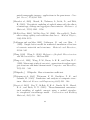
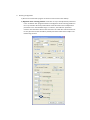
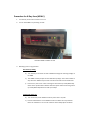
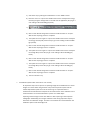
control application changes to “Ready”. PXE‐control application interface after warming up 4. Scanning configuration a) Run the “CT‐Rotate 225” program. A shortcut can be found on the desktop. b) Alignment of the scanning platform: A red value on any of the adjustment parameters in the “CT‐Rotate 225” program indicates a misalignment of the scanning platform in the x‐ray chamber. Necessary amendments should be made so that all adjustment parameters are in the allowable range. For instance, the “table tilt” parameter relates to how the table is tilted in the horizontal. The “table tilt” value should be set to zero (0) to ensure that the table is perfectly horizontal and that the sample is not tilted during the scan. “CT‐Rotate 225” application interface c) Alignment of the x‐ray source and the detector: The scanning should be carried out in a way that the full image of the object/sample can be captured on the detector. The x‐ray source, detector and scanning platform can be aligned using the control gear. The control gear is a variable speed Joystick used to control all drives. Each axis control is independent allowing simultaneous movement of all axis. Control gear with variable speed joystick d) Once the object has been placed on the scanning platform, and the necessary alignments have been made, then the actual scanning can be carried out. 5. Scanning a sample a) Push the “225kV Enable” button on the main console. b) Open the FXE‐Control application window and then click “X‐ray On” to start the emission of x‐ray. c) Check if the full image is formed on detector and if not, you have to make necessary alignment changes. These changes can be made using the control gear. The process of re‐alignment of the detector, X‐ray source and the scanning platform can be monitored using the CCTV monitor outside the scanning chamber. There are four cameras installed in the scanning chamber. Changing the Scan settings: The energy intensity at which the scan is to be performed can be changed on the “FXE‐Control” application while the setting of the amount of details to capture can be changed on the “CT‐rotate 225“application. a) Settings on the FXE‐Control application: The scanning voltage and current can be adjusted by moving the voltage slider and current slider. The sliders for the voltage and the current are independent of each other. The voltage corresponds to the energy intensity of the X‐ray. The adjustment should be made until one gets a good scan image on the computer screen. A too dark image implies a bad scan and a too light image indicates that some details might have been lost during the scan. This process is very important in the scan process and requires the judgment of the person carrying out the scan. The linear attenuation coefficient of the materials to be scanned can be used to get an idea of the appropriate energy level required for the scan. The changes made to the energy intensities are immediately reflected on the image on the computer screen. b) Settings on the CT‐rotate 225: Change the number of frames per second (fps) to a suitable value. This is directly related to how much detail you like to capture during the scan. A fps of 2 is usually ideal for small objects, but a fps greater than 2 will be suggested for large objects like asphalt cores. There is a tradeoff between scanning‐speed and scan quality when considering the number of frames per second. When you change the value of the fps, check the image on the computer screen if it is satisfactory before proceeding. If the image is satisfactory, then turn off the X‐Ray emission by pushing the “enable x‐ray” to turn off the x‐ray. Scanning a) After necessary change in the scanning configuration and the scan settings, the actual scanning process follows. b) To start a new scan, click on CT‐Project On the CT‐rotate 225 application window and the CT‐Project window opens. c) On the CT‐Project window, select a location to save the new scan, make a new folder and give a name to the new folder. Then click “OK”. d) Click on CT‐Scan to start the scanning process. Then wait till the scan is finished. e) Turn off the X‐ray and take out the object from the scanning chamber. f)
Scanning is completed. 6. Detector Calibration The two principal signal calibrations are offset and gain, which determine the detector readings with X‐rays off, and with X‐rays on at scanning conditions, respectively (Cite Ketcham) Click on Detector Calibration, configure offset map, detective pixels, and change No. of frames acquired to 200. The number of frames refers to the number of slices required from the scanned sample. (*) To get rid of defective pixels on the detector, we need to take the following steps to make necessary corrections. a) Start the X‐ray by pushing the “Enable 225kV” button on the main console. b) Place the cursor on a spot in the middle of the screen and adjust the energy intensity (using the voltage slider in the FXE‐control application) till you get a raw reading of about 60 000 (grey levels). c)
d) Click on Gain #0 and change the # of frames to 200 and click on “acquire”. Wait for the acquiring process to complete. e) Then place the cursor again on a spot in the middle of the screen and adjust the energy intensity like previous till you get a raw reading of about 45 000 (grey levels). f) Click on Gain #1 and change the # of frames to 200 and click on “acquire”. Wait for the acquiring process to complete. g) Then place the cursor again on a spot in the middle of the screen and adjust the voltage like previous till you get a raw reading of about 30 000 (grey levels). h) Click on Gain #2 and change the # of frames to 200 and click on “acquire”. Wait for the acquiring process to complete. i) Then place the cursor again on a spot in the middle of the screen and adjust the voltage like previous till you get a raw reading of about 15 000 (grey levels). j) Click on Gain #3 and change the # of frames to 200 and click on “acquire”. Wait for the acquiring process to complete. k) Then turn off the X‐ray. 7. CT Calibration (Notes taken from efX‐CT user manual) An important step in the CT process is capturing images of the calibration tool. These images are used to define the geometric setup of the inspection system and the relationship between pixels and units of measuring. It is imperative that no movements be made with the exception of the rotational axis. If the calibrations tool needs elevation it is recommended that it is place on a stable object. Capturing of these images can be done before or after capturing of the inspection radiographs. Additionally, the energies and filters used during acquisition may be altered for the calibration images. The idea is to maximize the contrast between the calibration spheres and the background. Positioning the Calibration Tool Positioning the calibration tool will require a degree of trial and error. The ideal situation will be to have the calibration tool travel from edge to edge of the image during a single 360 degree of rotation. The balls of the calibration tool must be at least 1 ball diameter from the edge of the image. It is also beneficial but not necessary to have the calibration tool reach from the bottom of the detector to the top. If the tool does not span from the top to the bottom, place the tool so that one portion of it reaches the top or bottom. This allows the creation of larger ellipses during rotation and better data for the software to build the volume off of. CT calibration procedure a) Place the calibration rod on the scanning platform. There are three sizes of calibration tools to choose from; large medium and small. Tool size used is determined by the magnification used during acquisition and detector size. b) On CT‐Project window, click on “CT Calib” and select the 15mm large tool (if you are using the large tool for the calibration else choose what corresponds to your choice) and then click “OK”. Then the calibration process begins. c) NB: Before the calibration process begins, necessary re‐alignment of the scanning platform might be required to make sure that the full image of the calibrating tool is captured on the detector. d) Wait for the calibration process to finish. Take note of the Calibration tool images above. These stills are 180 degrees apart from one another. The last item to note is the number of calibration spheres visible. The more of them present, the more accurate the software will interpret the geometric positioning of the x‐ray tube, detector, and manipulator. 225kv X‐ray energy generator This is the end of the Scan. Procedure for X‐Ray Scan (450kV) 1. Turn the key on the main console to turn on. 2. Turn on the 450kV X‐ray scanning console. KTH NSI X‐5000 CT 450kV console 3. Warming up the x‐ray generator Pre‐warm up setting d) Turn the key on the main console to 450kV t0 change the scanning voltage on to 450kV e) The 450kV console prompts for the downtime (in days). This is the number of days since the 450kV X‐ray was last used. Enter the value for the downtime. f)
Press Ctrl+1, then enter “101” to change to short warm‐up mode (Mod 101). Short warm‐up takes about 15mins while the option 102 is for the long warm‐
up mode (Mod 102) which can take up to 2days. To begin the warm‐up d) Turn on the key on the 450kV console to power the x‐ray tube. e) Press the black button on the 450kV console to initiate the X‐ray emission. Note: the red button is to turn off emission. Note: Always place the beam blocker in front of the x‐ray source to block the rays from getting to the detector during warm‐up, if this is not done then the x‐rays can damage the detector. f)
The pre‐warming process begins and continues until the voltage increases to 450kV. g) When the voltage reaches 450kV, then the warm‐up process is completed. 4. Scanning configuration e) Run the “CT‐Rotate 450” program. A shortcut can be found on the desktop. f) Alignment of the scanning platform: A red value on any of the adjustment parameters in the “CT‐Rotate 450” program indicates a misalignment of the scanning platform in the x‐ray chamber. Necessary amendments should be made so that all adjustment parameters are in the allowable range. For instance, the “table tilt” parameter relates to how the table is tilted in the horizontal. The “table tilt” value should be set to zero (0) to ensure that the table is perfectly horizontal and that the sample is not tilted during the scan. “CT‐Rotate 450” application interface g) Alignment of the x‐ray source and the detector: The scanning should be carried out in a way that the full image of the object/sample can be captured on the detector. The x‐ray source, detector and scanning platform can be aligned using the control gear. The control gear is a variable speed Joystick used to control all drives. Each axis control is independent allowing simultaneous movement of all axis. h) Once the object has been placed on the scanning platform, and the necessary alignments have been made, then the actual scanning can be carried out. 5. Scanning a sample d) Run the “CT‐Rotate 450” program. A shortcut can be found on the desktop. e) Push the “450kV Enable” button on the main console to turn X‐ray ON. f)
Check if the full image is formed on detector and if not, you have to make necessary alignment changes. These changes can be made using the control gear. The process of re‐alignment of the detector, X‐ray source and the scanning platform can be monitored using the CCTV monitor outside the scanning chamber. There are four cameras installed in the scanning chamber. Changing the Scan settings: The voltage and the current to perform the scan can be changed on the 450kV console while the setting of the amount of details to capture can be changed on the “CT‐rotate 450“ application. a) Settings on 450kV console: The voltage and the current for the 450kV scan can be adjusted to obtain a good scanned image. On the 450kV console, press the kV or mA button and turn the knob to adjust the voltage and the current respectively until a satisfactory image is obtained. The voltage corresponds to the energy intensity of the X‐ray. The adjustment should be made until one gets a good scan image on the computer screen. A too dark image implies a bad scan and a too light image indicates that some details might have been lost during the scan. This process is very important in the scan process and requires the judgment of the person carrying out the scan. The linear attenuation coefficient of the materials to be scanned can be used to get an idea of the appropriate energy level required for the scan. The changes made to the energy intensities are immediately reflected on the image on the computer screen. b) Settings on the CT‐rotate 450: Change the number of frames per second (fps) to a suitable value. This is directly related to how much detail you like to capture during the scan. A fps of 2 is usually ideal for small objects, but a fps greater than 2 will be suggested for large objects like asphalt cores. There is a tradeoff between scanning‐
speed and scan quality when considering the number of frames per second. When you change the value of the fps, check the image on the computer screen if it is satisfactory before proceeding. If the image is satisfactory, then push the “red button” on the 450kV console to turn X‐ray OFF. Scanning a) After necessary change in the scanning configuration and the scan settings, the actual scanning process follows. b) To start a new scan, click on CT‐Project On the CT‐rotate 450 application window and the CT‐Project window opens. c) On the CT‐Project window, select a location to save the new scan, make a new folder and give a name to the new folder. Then click “OK”. d) Click on CT‐Scan to start the scanning process. Then wait till the scan is finished. e) Turn off the X‐ray and take out the object from the scanning chamber. f)
Scanning is completed. 6. Detector Calibration The two principal signal calibrations are offset and gain, which determine the detector readings with X‐rays off, and with X‐rays on at scanning conditions, respectively (Cite Ketcham) Click on Detector Calibration, configure offset map, detective pixels, and change No. of frames acquired to 200. The number of frames refers to the number of slices required from the scanned sample. (*) To get rid of defective pixels on the detector, we need to take the following steps to make necessary corrections. a) Start the X‐ray by pushing the “black button” on the 450kV console. b) Place the cursor on a spot in the middle of the screen and adjust the energy intensity (using the voltage slider in the FXE‐control application) till you get a raw reading of about 60 000 (grey levels). c)
d) Click on Gain #0 and change the # of frames to 200 and click on “acquire”. Wait for the acquiring process to complete. e) Then place the cursor again on a spot in the middle of the screen and adjust the energy intensity like previous till you get a raw reading of about 45 000 (grey levels). f) Click on Gain #1 and change the # of frames to 200 and click on “acquire”. Wait for the acquiring process to complete. g) Then place the cursor again on a spot in the middle of the screen and adjust the voltage like previous till you get a raw reading of about 30 000 (grey levels). h) Click on Gain #2 and change the # of frames to 200 and click on “acquire”. Wait for the acquiring process to complete. i) Then place the cursor again on a spot in the middle of the screen and adjust the voltage like previous till you get a raw reading of about 15 000 (grey levels). j) Click on Gain #3 and change the # of frames to 200 and click on “acquire”. Wait for the acquiring process to complete. k) Then turn off the X‐ray. 7. CT Calibration (Notes taken from efX‐CT user manual) An important step in the CT process is capturing images of the calibration tool. These images are used to define the geometric setup of the inspection system and the relationship between pixels and units of measuring. It is imperative that no movements be made with the exception of the rotational axis. If the calibrations tool needs elevation it is recommended that it is place on a stable object. Capturing of these images can be done before or after capturing of the inspection radiographs. Additionally, the energies and filters used during acquisition may be altered for the calibration images. The idea is to maximize the contrast between the calibration spheres and the background. Positioning the Calibration Tool Positioning the calibration tool will require a degree of trial and error. The ideal situation will be to have the calibration tool travel from edge to edge of the image during a single 360 degree of rotation. The balls of the calibration tool must be at least 1 ball diameter from the edge of the image. It is also beneficial but not necessary to have the calibration tool reach from the bottom of the detector to the top. If the tool does not span from the top to the bottom, place the tool so that one portion of it reaches the top or bottom. This allows the creation of larger ellipses during rotation and better data for the software to build the volume off of. CT calibration procedure a) Place the calibration rod on the scanning platform. There are three sizes of calibration tools to choose from; large medium and small. Tool size used is determined by the magnification used during acquisition and detector size. b) On CT‐Project window, click on “CT Calib” and select the 15mm large tool (if you are using the large tool for the calibration else choose what corresponds to your choice) and then click “OK”. Then the calibration process begins. TSC-MT 13-002
www.kth.se