Download vignette

142
143
144
145
146
147
148
149
107
109
110
150
111
50
112
29
79
153
114
154
14
52
81
115
155
54
17
55
118
158
18
56
84
57
119
159
58
120
160
126
124
129
92
127
125
123
122
162
62
90
88
130
93
91
89
87
121
161
38
60
131
94
63
61
59
86
64
20
36
132
95
39
37
35
85
40
8
133
96
65
21
19
34
66
22
2
134
97
41
9
7
33
83
117
157
1
16
42
10
135
98
67
23
3
6
32
82
116
156
5
31
43
11
136
99
68
24
4
15
53
44
12
137
100
69
25
13
30
80
45
27
138
101
70
26
28
51
113
46
48
139
102
71
47
49
78
152
72
74
76
140
103
73
75
77
151
105
106
108
141
104
128
169
168
167
166
165
164
163
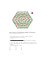
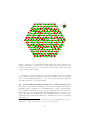
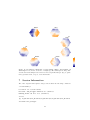
Figure 1: A supra-hexagonal map. It consists of nHex = 169 smaller
hexagons. For easy reference, these hexagons are indexed according to: firstly,
how many steps a hexagon is away from the grid centroid (’1’ for the centroid
itself); secondly, for those hexagons of the same step, an anti-clock order starting from the rightmost. This map can also be easily described by the grid
radius (i.e., the maximum steps away from the centroid; r = 8 in this case), or
by the xy-dimensions of the map grid (i.e., the maximum number of hexagons
horizontally/vertically; xdim = ydim = 15 in this case).
map node is associated with two coordinates: one in two-dimensional output
space just as you have seen; the other in high-dimensional input space as you
can imagine. The coordinate in input space is represented as a prototype/weight
vector (with the same dimension as input data vector). Prototype vectors in
all map nodes collectively form the codebook matrix. In essence, the suprahexagonal map converts the input data into the codebook matrix. In terms
of gene activity matrix as input, supraHex produces a map, wherein (i) genes
with the same or similar activity patterns are spatially located/clustered to the
same or nearby map nodes, (ii) the density of genes mapped onto this map
(i.e. what we can see) is an equivalent to the data density in high-dimensional
input space (i.e. what we can only imagine), and (iii) when all map nodes
are color-coded according to values in a specific component for all prototype
vectors (i.e. a specific column of codebook matrix), a color-coded component
map can be used to illustrate sample-specific gene activities, and thus multiple
components illustrate changes across all samples in subject. Owing to these
unique features, the supra-hexagonal map can be used for gene clustering and
sample representation.
4