1
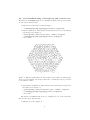
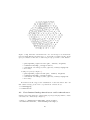
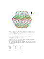
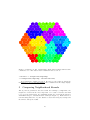
supraHex : an R/Bioconductor package for
tabular omics data analysis using a
supra-hexagonal map
Hai Fang∗, Julian Gough
Department of Computer Science
University of Bristol, UK
Abstract
We introduce an R/Bioconductor package called supraHex 1 . It names after a supra-hexagon that is a giant hexagon on a 2-dimensional (2D) map
grid seamlessly consisting of smaller hexagons. This 2D giant hexagon is
intended to train, analyse and visualise a high-dimensional omics data,
which usually involves a large number of genomic coordinates (e.g. genes)
but a much smaller number of samples. The resulting supra-hexagon ensembles the structure of the input data in a topology-preserving fashion.
With the supraHex, users are able to easily and intuitively carry out integrated tasks such as: simultaneous analysis of gene clustering and sample
correlation, and the overlaying of additional data (if any) onto the map
for multilayer omics data comparisons. In this vignette/guide, we give a
tutorial-style introduction into how the functions contained in the package
supraHex can be used to better understand the input omics data. This
vignette assumes some basic familiarity with the R language and environment. It only provides a task-oriented description of the package functionality, and compliments the accompanying manual ’supraHex-manual.pdf’
that gives a full description of all functions.
∗ [email protected]
1 http://suprahex.r-forge.r-project.org
1
Contents
1 Introduction
1.1 What is supraHex ? . . . . . . . . . . . . . . . . . . . . . . . . . .
1.2 Why to use supraHex ? . . . . . . . . . . . . . . . . . . . . . . . .
1.3 How to interpret supraHex ? . . . . . . . . . . . . . . . . . . . . .
3
3
3
3
2 Installation and Citation
5
3 Quick Overview
6
4 Main Functionality
4.1 Get trained using sPipeline . . . . . . . . . . . . . . . .
4.2 Get visualised using visHexMapping and visHexPattern
4.3 Get clustered using sDmatCluster and visDmatCluster .
4.4 Get reordered using sCompReorder and visCompReorder .
.
.
.
.
.
.
.
.
.
.
.
.
.
.
.
.
5 Comparing Neighborhood Kernels
7
8
9
10
12
13
6 Applications to Real Cases
17
6.1 Leukemia patient dataset from Golub et al . . . . . . . . . . . . 18
6.2 Human embryo dataset from Fang et al . . . . . . . . . . . . . . 19
6.3 Arabidopsis embryo dataset from Xiang et al . . . . . . . . . . . 19
7 Session Information
21
List of Tables
1
2
A summary of functions used for training and analysis .
A summary of functions used for visualisation . . . . . .
6
7
List of Figures
1
2
3
4
5
6
7
8
9
10
11
12
13
14
15
16
A supra-hexagonal map . . . . . . . . . . . . . . . . . . . . . . .
Map hit distribution . . . . . . . . . . . . . . . . . . . . . . . . .
Map distance visualisation . . . . . . . . . . . . . . . . . . . . . .
Line plot of codebook patterns . . . . . . . . . . . . . . . . . . .
Bar plot of codebook patterns . . . . . . . . . . . . . . . . . . . .
Clusters of the trained map . . . . . . . . . . . . . . . . . . . . .
Reordered components of trained map . . . . . . . . . . . . . . .
Neighborhood kernels . . . . . . . . . . . . . . . . . . . . . . . .
Components of trained map with the gaussian kernel . . . . . . .
Components of trained map with the bubble kernel . . . . . . . .
Components of trained map with the cutgaussian kernel . . . . .
Components of trained map with the ep kernel . . . . . . . . . .
Components of trained map with the gamma kernel . . . . . . .
Reordered components of map for leukemia classification . . . . .
Reordered components of map during early human organogenesis
Reordered components of map during embryo development in
Arabidopsis . . . . . . . . . . . . . . . . . . . . . . . . . . . . . .
2
4
9
10
11
12
13
14
15
15
16
16
17
17
18
20
21
1
Introduction
1.1
What is supraHex ?
The supraHex package (Fang and Gough, 2014) devises a supra-hexagonal map.
This map consists of smaller hexagonal lattices on a regular 2-dimensional (2D)
grid; these smaller hexagons collectively form a giant hexagon (see Figure 1).
As seen, it has symmetric beauty around the center, from which individual
hexagons radiate outwards. To ensure that a supra-hexagon is forme dexactly,
inherent relationships must be met between the total number nHex of hexagons
in the grid, the grid radius r, and the xy-dimensions xdim and ydim:
• nHex = 1 + 6 ∗ r ∗ (r − 1)/2;
• xdim = ydim = 2 ∗ r − 1.
The codes used to produce this example are (assumedly the package has
been successfully installed; see Section 2):
>
>
>
>
>
library("supraHex")
pdf("supraHex_vignettes-suprahex.pdf", width=6, height=6)
sTopol <- sTopology(xdim=15, ydim=15, lattice="hexa", shape="suprahex")
visHexMapping(sTopol,mappingType="indexes",newpage=F)
dev.off()
1.2
Why to use supraHex ?
Biologists are far often confronted with ever-increasing amounts of omics data
that are tabulated in the form of matrix, measuring levels/activities of genomic
coordinates (e.g. genes) against experimental samples. The matrix usually involves tens of thousands of genes but a much smaller number of samples (at
most hundreds), known as ’small-sample-but-large-gene’. The atypical structure requires easy-to-interpret models. Unsupervised learning algorithm/model
such as self-organising map is popular for its unique way in capturing input data
patterns, this is, simultaneously performing vector quantisation but regularised
by vector projection. The supraHex borrows this learning algorithm to produce
a supra-hexagonal map (two-dimensional output space) from input omics data
( high-dimensional input space). In this map, geographically close locations are
indicative of patterns that are similar in terms of the input space. Thanks to the
prevalence in nature and symmetric beauty, this supra-hexagonal map is probably suited for analysing such input data with approximately perfect symmetry.
We argue that omics data tend to be symmetric due to unbiased measurements
of gene levels/activities on a global scale. Even when priori knowledge of the
data symmetry is unknown, we also argue that at least the supra-hexagonal
map can provide the ease with visualisation.
1.3
How to interpret supraHex ?
As a result of training, similar input data are mapped onto neighboring regions of
the supra-hexagonal map. More formally, the map ensembles the structure (the
shape and density) of the input data in a topology-preserving fashion. Each
3
142
143
144
145
146
147
148
149
107
109
110
150
111
50
112
29
79
153
114
154
14
52
81
115
155
54
17
55
118
158
18
56
84
57
119
159
58
120
160
126
124
129
92
127
125
123
122
162
62
90
88
130
93
91
89
87
121
161
38
60
131
94
63
61
59
86
64
20
36
132
95
39
37
35
85
40
8
133
96
65
21
19
34
66
22
2
134
97
41
9
7
33
83
117
157
1
16
42
10
135
98
67
23
3
6
32
82
116
156
5
31
43
11
136
99
68
24
4
15
53
44
12
137
100
69
25
13
30
80
45
27
138
101
70
26
28
51
113
46
48
139
102
71
47
49
78
152
72
74
76
140
103
73
75
77
151
105
106
108
141
104
128
169
168
167
166
165
164
163
Figure 1: A supra-hexagonal map. It consists of nHex = 169 smaller
hexagons. For easy reference, these hexagons are indexed according to: firstly,
how many steps a hexagon is away from the grid centroid (’1’ for the centroid
itself); secondly, for those hexagons of the same step, an anti-clock order starting from the rightmost. This map can also be easily described by the grid
radius (i.e., the maximum steps away from the centroid; r = 8 in this case), or
by the xy-dimensions of the map grid (i.e., the maximum number of hexagons
horizontally/vertically; xdim = ydim = 15 in this case).
map node is associated with two coordinates: one in two-dimensional output
space just as you have seen; the other in high-dimensional input space as you
can imagine. The coordinate in input space is represented as a prototype/weight
vector (with the same dimension as input data vector). Prototype vectors in
all map nodes collectively form the codebook matrix. In essence, the suprahexagonal map converts the input data into the codebook matrix. In terms
of gene activity matrix as input, supraHex produces a map, wherein (i) genes
with the same or similar activity patterns are spatially located/clustered to the
same or nearby map nodes, (ii) the density of genes mapped onto this map
(i.e. what we can see) is an equivalent to the data density in high-dimensional
input space (i.e. what we can only imagine), and (iii) when all map nodes
are color-coded according to values in a specific component for all prototype
vectors (i.e. a specific column of codebook matrix), a color-coded component
map can be used to illustrate sample-specific gene activities, and thus multiple
components illustrate changes across all samples in subject. Owing to these
unique features, the supra-hexagonal map can be used for gene clustering and
sample representation.
4
2
Installation and Citation
supraHex is a package for the R computing environment and it is assumed that
you have already installed the latest version of R (>=3.0.2). You can install
the package following step-by-step guidelines in http://suprahex.r-forge.
r-project.org. Briefly, you can install it from Bioconductor (or R-Forge):
Using the release version2 (officially released on 15-10-2013):
> source("http://bioconductor.org/biocLite.R")
> biocLite("supraHex")
> library(supraHex) # load the package
Using the latest development version3 (prefer it for the benefit of latest improvements):
> install.packages("hexbin",repos="http://www.stats.bris.ac.uk/R")
> install.packages("supraHex",repos="http://R-Forge.R-project.org", type="source")
> library(supraHex) # load the package
To get help information for the package, please type one of two commands:
> library(help="supraHex") # real-time help
> help.start() # html help (follow the links to supraHex)
To view this vignette source and R code whereof, please type:
> browseVignettes("supraHex")
supraHex is free to use under GPL 2. You can get citation information from:
> citation("supraHex") # cite the package
Please cite this package as:
Fang H, Gough J. (2014) supraHex: an R/Bioconductor package for tabular omics data
analysis using a supra-hexagonal map. Biochemical and Biophysical Research Communications, 443(1), 285-289. DOI: http://dx.doi.org/10.1016/j.bbrc.2013.11.103, PMID:
http://www.ncbi.nlm.nih.gov/pubmed/?term=24309102
2 http://bioconductor.org/packages/release/bioc/html/supraHex.html
3 http://bioconductor.org/packages/devel/bioc/html/supraHex.html
5
3
Quick Overview
The functions in the package supraHex are divided into two categories: one for
training and analysis (see Table 1), the other for visualisation (see Table 2).
Table 1: A summary of functions used for training and analysis
Function
sHexGrid
sTopology
sHexGrid
sInitial
Description
Define a supra-hexagonal grid; return a list.
Define the topology of a map grid; return a sTopol object.
Define a supra-hexagonal grid; return a list.
Initialise a sMap object given a topology and input data; return a
sMap object.
sTrainology Define trainology (training environment); return a sTrain object.
sTrainSeq
Implement training via sequential algorithm; return a sMap object.
sTrainBatch Implement training via batch algorithm; return a sMap object.
sBMH
Identify the best-matching hexagons for the input data; return a
list.
sPipeline
Setup the pipeline for completing ab initio training given the input
data; return a sMap object.
sNeighDirect Calculate direct neighbors for each hexagon in a grid; return a
matrix.
sNeighAny
Calculate any neighbors for each hexagon in a grid; return a matrix.
sHexDist
Calculate distances between hexagons in a 2D grid; return a matrix.
sDistance
Compute the pairwise distance for a given data matrix; return a
matrix.
sDmat
Calculate distance matrix in high-dimensional input space but according to neighborhood relationships in 2D output space; return
a vector.
sDmatMinima Identify local minima (in 2D output space) of distance matrix (in
high-dimensional input space); return a vector.
sDmatCluster Partition a grid map into clusters; return a list.
sCompReorder Reorder component planes; return a sReorder object.
sWriteData
Write out the best-matching hexagons and/or cluster bases in terms
of data; return a data frame.
sMapOverlay Overlay additional data onto the trained map; return a sMap object.
6
Table 2: A summary of functions used for visualisation
Function
visHexGrid
visHexMapping
visHexComp
visColormap
visColorbar
visVp
visHexMulComp
visCompReorder
Description
Visualise a supra-hexagonal grid.
Visualise various mapping items within a supra-hexagonal grid.
Visualise a component plane of a supra-hexagonal grid.
Define a colormap.
Define a colorbar.
Create viewports for multiple supra-hexagonal grids.
Visualise multiple component planes of a supra-hexagonal grid.
Visualise multiple component planes reorded within a sheet-shape
rectangle grid.
visHexPattern Visualise codebook matrix or input patterns within a suprahexagonal grid.
visDmatCluster Visualise clusters/bases partitioned from a supra-hexagonal grid.
visKernels
Visualize neighborhood kernels.
4
Main Functionality
This vignette aims to demonstrate the functionality of the package supraHex
in utilising the supra-hexagonal map to train, analyse and visualise a highdimensional omics data. To simplify the descriptions, it deals with the gene
expression data. But it can also be applied in any other omics data, a tabular
matrix usually containing thousands of genes but with at most hundreds of
samples. Assumedly, we have a gene expression matrix of 1000×6, measuring the
expression levels of 1000 genes across 6 samples. These samples come from two
different normal distributions (S1 and S2), and each (i.e., a matrix of 1000 × 3)
is randomly generated from the same normal distribution. All examples below
are based on the latest development version4 .
>
+
+
+
>
data <- cbind(
matrix(rnorm(1000*3,mean=0.5,sd=1), nrow=1000, ncol=3),
matrix(rnorm(1000*3,mean=-0.5,sd=1), nrow=1000, ncol=3)
)
colnames(data) <- c("S1","S1","S1","S2","S2","S2")
The first 5 rows of this data:
> data[1:5,]
[1,]
[2,]
[3,]
[4,]
[5,]
S1
S1
S1
S2
S2
S2
-0.04637505 -1.5331183 -0.4571943 -1.4867335 -0.29145199 -1.7896765
-0.12146664 1.4618621 -0.4696756 0.1062753 -0.61200805 -0.8049917
1.43196516 0.8075947 -1.0812769 -0.5381012 -0.47702965 1.7736551
-0.05503947 0.3613781 1.1981018 -0.4531657 0.02479884 0.4235951
-0.58916751 -0.5537234 1.6807673 0.8336744 -0.67680705 0.7072746
4 http://bioconductor.org/packages/devel/bioc/html/supraHex.html
7
You can prepare your own data (a tab-delimited text file). Similarly as
shown above, this file should contain the first row intended for sample names,
the first column for gene names, and the top-left entry being left empty. You
can import it using the R built-in function read.table:
> data <- read.table(file="you_input_data_file", header=T, row.names=1, sep="\t")
4.1
Get trained using sPipeline
The function sPipeline setups the pipeline for completing ab initio training
given the input data only. It sequentially consists of:
1. sTopology used to define the topology of a grid (with ”suprahex” shape
by default ) according to the input data;
2. sInitial used to initialise the codebook matrix given the pre-defined
topology and the input data (by default using ”uniform” initialisation
method);
3. sTrainology and sTrainSeq used to get the grid map trained at both
”rough” and ”finetune” stages. If instructed, sustain the ”finetune” training
until the mean quantization error does get worse;
4. sBMH used to identify the best-matching hexagons/rectangles (BMH) for
the input data, and these response data are appended to the resulting
object of ”sMap” class.
Below is its common usage of sPipeline with default setup (using gaussian
kernel and printing out messages in the screen):
> sMap <- sPipeline(data=data)
Use sWriteData to write out the best-matching hexagons in terms of data
(equivalent to gene clustering):
> # it will also write out a file ('Output.txt') into your disk
> output <- sWriteData(sMap=sMap, data=data, filename="Output.txt")
> output[1:5,]
1
2
3
4
5
ID Hexagon_index
1
148
2
66
3
59
4
54
5
73
You will see: the first column for your input data ID (an integer; otherwise
the row names of input data matrix), and the second column for the corresponding index of best-matching hexagons (i.e. gene clusters). On the way how
hexagons get indexed, please refer to Figure 1.
8
4.2
Get visualised using visHexMapping and visHexPattern
The function visHexMapping is used to visualise the single-value properties that
are associated with the map:
• map indexes as shown previously in Figure 1.
> visHexMapping(sMap,mappingType="indexes",newpage=F)
• map hit distribution, which tells how many input data vectors are hitting
each hexagon (see Figure 2).
> pdf("supraHex_vignettes-hit.pdf", width=6, height=6)
> visHexMapping(sMap,mappingType="hits",newpage=F)
> dev.off()
8
14
5
9
9
13
6
8
7
3
5
6
8
8
4
3
10
6
5
3
10
4
6
2
3
5
4
7
7
4
11
6
4
4
6
5
11
4
5
2
4
2
7
4
7
8
6
5
0
5
12
1
3
6
3
3
3
3
7
5
5
2
2
4
8
6
5
8
10
15
2
4
4
3
1
9
10
3
9
8
9
1
7
3
15
2
5
3
4
5
8
6
8
10
8
4
1
4
3
7
4
7
8
1
6
4
13
3
6
5
2
7
4
4
9
11
2
7
3
11
7
6
4
2
6
6
5
12
1
6
5
2
5
4
9
9
7
4
7
5
2
9
7
10
8
3
4
2
6
6
6
10
7
8
3
6
4
5
2
5
9
11
9
8
10
9
5
8
14
Figure 2: Map hit distribution. The number represents how many input
data vectors are hitting each hexagon. The size of each hexagon is proportional
to the number of hits.
• map distance visualisation, which tells how far each hexagon is away from
its neighbors (see Figure 3).
> pdf("supraHex_vignettes-distance.pdf", width=6, height=6)
> visHexMapping(sMap,mappingType="dist",newpage=F)
> dev.off()
The function visHexPattern is used to visualise the vector-based patterns
that are associated with the map:
• using line plots (see Figure 4).
9
Figure 3: Map distance visualisation. For each hexagon, its median distances in high-dimensional input space to its neighbors (defined in 2D output
space) is calculated. The size of each hexagon is proportional to this distance.
>
>
+
>
pdf("supraHex_vignettes-line.pdf", width=6, height=6)
visHexPattern(sMap, plotType="lines",
customized.color=rep(c("red","green"),each=3),newpage=F)
dev.off()
• using bar plots (see Figure 5).
>
>
+
>
pdf("supraHex_vignettes-bar.pdf", width=6, height=6)
visHexPattern(sMap, plotType="bars",
customized.color=rep(c("red","green"),each=3),newpage=F)
dev.off()
Both functions also support the visualisation of user-customised data. On
this advanced usage, please refer to specifications of functions by:
> ?visHexMapping
> ?visHexPattern
4.3
Get clustered using sDmatCluster and visDmatCluster
Partition the trained map into clusters using region-growing algorithm to ensure
each cluster is continuous (see Figure 6).
> sBase <- sDmatCluster(sMap=sMap, which_neigh=1,
+ distMeasure="median", clusterLinkage="average")
10
●
● ●
●
●
● ●
●
● ●
●
●
● ●
● ●
● ●
●
●
● ●
●
●
●
●
●
● ●
●
●
●
●
● ●
●
● ●
●
●
●
●
●
● ●
●
●
●
●
●
●
●
●
●
●
●
● ●
●
●
●
●
●
●
●
●
●
● ●
●
●
● ● ●
●
●
●
●
●
●
●
●
● ●
●
●
● ● ●
●
● ●
●
●
●
●
●
●
●
● ●
●
●
●
●
●
●
●
●
●
●
●
●
●
●
●
●
●
● ●
●
●
●
● ●
●
●
●
●
●
●
●
●
●
●
● ●
●
●
●
●
●
●
●
●
●
●
●
●
●
●
●
●
●
●
●
●
● ●
●
●
● ●
● ●
●
●
●
●
● ●
●
●
●
●
●
●
● ●
● ●
●
●
●
●
●
●
●
● ●
● ●
● ●
●
●
●
●
●
●
● ●
●
●
●
●
●
●
● ●
●
●
● ●
●
●
●
●
● ●
●
●
●
●
●
●
●
●
●
●
●
●
●
● ●
● ●
●
●
●
●
● ●
●
●
●
●
●
●
● ●
●
●
●
●
●
●
●
●
●
●
●
●
● ●
●
●
●
●
● ●
●
● ●
●
●
●
●
● ● ●
●
●
● ●
●
●
●
●
●
●
● ●
●
●
●
● ●
●
●
● ●
●
●
●
●
● ● ●
● ● ●
●
●
●
●
●
●
●
● ●
●
●
●
●
●
●
●
●
●
●
●
●
● ●
●
●
● ●
● ●
●
●
●
●
●
●
●
●
●
●
● ● ●
● ●
●
●
●
●
● ●
●
●
●
●
●
●
● ● ●
●
●
●
●
●
●
●
●
●
●
●
●
● ●
●
●
●
●
●
● ●
● ●
●
● ●
●
● ●
●
●
●
●
●
●
●
● ●
●
● ● ●
●
●
●
●
●
● ●
●
●
●
●
●
●
●
●
● ●
●
●
●
●
●
●
● ●
●
●
● ●
●
●
● ●
●
● ●
●
●
●
●
●
●
●
●
●
●
●
●
●
●
●
●
●
● ●
●
●
●
●
● ●
●
●
●
●
●
●
●
●
●
●
●
● ●
●
●
●
● ●
●
●
●
●
●
●
●
●
●
●
●
●
●
●
●
●
●
●
● ●
●
●
●
●
● ●
●
●
●
●
● ●
● ●
●
●
●
● ●
●
●
●
●
●
●
●
● ●
●
●
●
●
●
●
●
●
● ●
●
●
●
● ●
●
●
●
●
●
●
●
●
● ●
●
● ●
●
●
● ●
●
●
●
● ●
● ●
●
●
●
●
● ●
●
●
●
●
● ●
●
●
●
●
●
●
●
●
● ●
●
●
●
●
●
●
●
●
●
●
●
●
●
●
● ●
●
● ●
●
● ●
●
●
●
●
●
●
●
● ● ●
●
●
●
● ●
●
●
●
●
●
●
●
●
●
● ●
●
●
●
●
● ●
●
● ●
●
● ●
●
● ●
● ●
●
S2
S2
●
●
●
●
● ●
●
●
●
● ●
● ●
●
●
●
●
●
●
●
● ●
●
●
● ●
●
●
●
●
● ● ●
●
●
●
● ●
●
●
● ●
S1
S2
● ●
● ● ●
●
●
●
●
●
●
●
●
●
●
● ● ●
S1
● ●
●
●
●
● ● ●
●
●
● ●
● ●
●
●
●
●
●
S1
●
●
●
●
●
●
● ●
●
● ●
●
●
●
●
● ●
● ●
●
●
● ●
●
●
● ●
●
●
● ●
●
●
●
●
●
●
●
●
●
●
●
●
●
●
●
●
● ●
● ● ●
● ●
●
●
● ●
●
●
●
●
●
● ●
●
●
●
●
●
● ●
● ●
●
●
●
●
●
●
●
●
●
●
●
● ● ●
●
●
●
●
● ● ●
● ●
●
●
●
●
●
●
● ●
●
●
●
● ●
●
●
●
●
●
●
● ●
●
●
●
● ●
●
●
●
● ●
●
● ●
● ● ● ●
●
●
● ●
●
●
●
●
● ●
●
●
●
●
●
● ●
●
●
●
●
● ●
●
●
●
● ●
● ● ●
● ●
●
● ●
● ●
●
●
●
●
●
● ●
● ●
●
●
●
●
●
●
●
●
●
● ●
●
●
●
● ●
● ●
● ● ● ●
●
● ●
●
●
●
● ●
●
●
● ●
● ●
●
●
●
●
●
●
●
● ●
●
●
●
●
●
●
● ●
●
●
●
●
●
●
●
●
●
●
●
●
● ●
● ●
●
●
●
● ●
●
● ●
●
●
●
●
●
●
● ●
●
Figure 4: Line plot of codebook patterns. If multple colors are given, the
points are also plotted. When the pattern involves both positive and negative
values, zero horizental line is also shown.
> pdf("supraHex_vignettes-cluster.pdf", width=6, height=6)
> visDmatCluster(sMap, sBase, newpage=F)
> dev.off()
It is equivalent to gene meta-clustering. Write out results into a tab-delimited
text file using sWriteData:
> # it will also write out a file ('Output_base.txt') into your disk
> output <- sWriteData(sMap, data, sBase, filename="Output_base.txt")
> output[1:5,]
1
2
3
4
5
ID Hexagon_index Cluster_base
1
148
2
2
66
17
3
59
10
4
54
5
5
73
14
11
S1
S1
S1
S2
S2
S2
Figure 5: Bar plot of codebook patterns. When the pattern involves both
positive and negative values, the zero horizental line is in the middle of the
hexagon; otherwise at the top of the hexagon for all negative values, and at the
bottom for all positive values.
You will see: the first column for your input data ID (an integer; otherwise
the row names of input data matrix), the second column for the corresponding
index of best-matching hexagons (i.e. gene clusters), and the third column for
the cluster bases (i.e. gene meta-clusters).
4.4
Get reordered using sCompReorder and visCompReorder
Reordering components for trained map can be realised by using a new map grid
(with sheet shape consisting of a rectangular lattice) to train component plane
vectors (either column-wise vectors of codebook/data matrix or the covariance
matrix thereof). As a result, similar component planes are placed closer to each
other. The functions sCompReorder and visCompReorder are respectively to
implement this reordering algorithm and to visualise the reordered compments
(see Figure 7)5 .
5 In
order to display colors properly, it is important to reset the argument ’zlim’ by respecting the range of input data matrix (more precisely, codebook matrix).
12
15
6
17
14
16
12
4
11
2
10
3
5
13
8
1
7
9
Figure 6: Clusters of the trained map. Each cluster is filled with the same
continuous color. The cluster index is marked in the seed node.
> sReorder <- sCompReorder(sMap=sMap)
> visCompReorder(sMap=sMap, sReorder=sReorder)
It is equivalent to sample projection. Reordered components are rich in the
information: both of genes and samples can be visualised but in a single display.
5
Comparing Neighborhood Kernels
Among various parameters associated with the training by sPipeline, the
neighborhood kernel is the most important one because it dictates the final
topology of the trained map. For visualising neighborhood kernels, the function
visKernels helps to understand their forms (see Figure 8). Each kernel is a
non-increasing functions of: i) the distance between the hexagon/rectangle and
the winner, and ii) the radius.
13
S1
S1
S2
S1
S2
S2
2
0
-2
Figure 7: Reordered components of trained map. Each component illustrates the sample-specific map and is placed within a two-dimensional rectangular lattice (framed in black). Within each component, genes with the same
or similar expression patterns are mapped to the same or nearby map nodes.
When zooming out to look at between-components/samples relationships, samples with the similar expression profiles are placed closer to each other.
> pdf("supraHex_vignettes-kernels.pdf", width=12, height=6)
> visKernels(newpage=F)
> dev.off()
From the mathematical definitions and curve forms above, it is clear that
the ”gamma” and ”gaussian” kernels exert more global influence, the ”ep” kernel puts more emphasis on local topological relationships, and the other two
”cutgaussian” and ”bubble” keep the relative balance. It becomes much clearer
when using the function visHexMulComp to visualise trained maps using the
same data input and the same trainology but choosing different kernels (see
Figure 9, Figure 10, Figure 11, Figure 12 and Figure 13)6 .
• with ”gaussian” kernel (see Figure 9)
> sMap_ga <- sPipeline(data=data, neighKernel="gaussian", init="uniform")
> visHexMulComp(sMap_ga)
• with ”bubble” kernel (see Figure 10)
> sMap_bu <- sPipeline(data=data, neighKernel="bubble", init="uniform")
> visHexMulComp(sMap_bu)
6 In order to display colors properly, it is important to reset the argument ’zlim’ by respecting the range of input data matrix (more precisely, codebook matrix).
14
●
●
0.6
bubble: hwi(t)=(dwi ≤ δt)
●
●
●
●
●
●
●
●
●
0.4
●
●
●
●
− d2wi
cutgaussian: hwi(t)=exp(
)(dwi ≤ δt)
2δ2t
2
dwi
gamma: hwi(t)=1 Γ(
+ 2)
4δ2t
●
●
●
●
●
●
●
●
●
●
●
●
0.0
1.0
●
●
●
●
●
●
●●
●●
●
●
●
●
● ●● ●●●
●●
● ● ●●
●●● ●●●●●●●●
●●●●●●●●●●●●●●●●●
0.8
●
●
0.6
●
●
− d2wi
gaussian: hwi(t)=exp(
)
2δt2
d2wi
ep: hwi(t)=(1 − )(dwi ≤ δt)
δt2
0.4
●
●
Neighborhood kernel hwi(t)
0.8
●
●
0.2
Neighborhood kernel hwi(t)
●
0.2
●●●
●
● ●●
●
●●
●
●
●
●
Radius δt=2
0.0
1.0
Radius δt=1
0
1
2
3
4
5
Distance dwi between the hexagon i and the winner w
●●●●●
●●
● ● ●● ●●
●●
●●●
●●
●
●●
●
●●
●
●●
●
●●
●
●
●
●
●
●
●
●
●
●
●
●
●
●
●
●
●
●
●
●
●
●
●
●
●
●
●
●
●
●
●
●
●
●
●
●
●
●
●
●
●
●
●
●
●
●
●
●
●
●
●
●
●
●
●
●
●
●
●
●●
●●
●●
●●
●●●
0
1
2
3
4
5
Distance dwi between the hexagon i and the winner w
Figure 8: Neighborhood kernels. There are five kernels that are currently
supported in the package supraHex. These kernels are displayed within a plot
for each fixed radius; two different radii (i.e. 1 and 2) are illustrated only.
S1
S1
S1
S2
S2
S2
2
0
-2
Figure 9: Components of trained map with the gaussian kernel.
• with ”cutgaussian” kernel (see Figure 11)
> sMap_cu <- sPipeline(data=data, neighKernel="cutgaussian", init="uniform")
> visHexMulComp(sMap_cu)
• with ”ep” kernel (see Figure 12)
> sMap_ep <- sPipeline(data=data, neighKernel="ep", init="uniform")
> visHexMulComp(sMap_ep)
15
S1
S1
S1
S2
S2
S2
2
0
-2
Figure 10: Components of trained map with the bubble kernel.
S1
S1
S1
S2
S2
S2
2
0
-2
Figure 11: Components of trained map with the cutgaussian kernel.
• with ”gamma” kernel (see Figure 13)
> sMap_gm <- sPipeline(data=data, neighKernel="gamma", init="uniform")
> visHexMulComp(sMap_gm)
16
S1
S1
S1
S2
S2
S2
2
0
-2
Figure 12: Components of trained map with the ep kernel.
S1
S1
S1
S2
S2
S2
2
0
-2
Figure 13: Components of trained map with the gamma kernel.
6
Applications to Real Cases
The most common real cases are applications in studies involving gene expression profilings of: i) clinical patients; ii) time-course processes. In this section,
we aim to showcase the applications by providing several datasets published
previously and a collection of functions (together with optimised arguments) to
analyse them. The end users are encouraged to adapt them to fit your dataset:
17
run them first, then get down to details. We do not repeat the explanations for
all used commands and output files and figures. On the meanings and interpretations, please refer to Section 4). On purpose of easy copying, all commands
are provided without the ’>’ prefix:
6.1
Leukemia patient dataset from Golub et al
This dataset (the learning set7 ) contains a 3051 × 38 matrix of expression levels, involving 3051 genes and two types of leukemia: 11 acute myeloid leukemia
(AML) and 27 acute lymphoblastic leukemia (ALL). These 27 ALL are further subtyped into 19 B-cell ALL (ALL B) and 8 T-cell ALL (ALL T) (see
Figure 14).
ALL_
T
ALL_
T
ALL_
T
ALL_
T
ALL_
T
AL L _
B
ALL_
B
ALL_
B
B
B
B
AL L _
B
AL L _
B
ALL_
T
ALL_
ALL_
AL L _
B
AL L _
B
AL L _
B
AL L _
B
AL L _
B
AL L _
ALL_
T
B
AML
AML
AML
AML
ALL_
ALL_
AL L _
AML
AL L _
ALL_
T
B
B
B
AML
AML
AML
AML
ALL_
B
AL L _
B
AML
AML
11
9
7
Figure 14: Reordered components of map for leukemia classification.
Each component illustrates a sample-specific transcriptome map. Geometric
locations of components display the relationships between 38 leukemia samples.
AML: acute myeloid leukemia; ALL: acute lymphoblastic leukemia; ALL B:
B-cell ALL; ALL T: T-cell ALL.
# import data
data(Golub)
data <- Golub
7 http://www.ncbi.nlm.nih.gov/pubmed/10521349
18
# get trained
sMap <- sPipeline(data)
visHexMulComp(sMap,title.rotate=10,
colormap="darkgreen-lightgreen-lightpink-darkred")
sWriteData(sMap, data, filename="Output_Golub.txt")
# get visualised
visHexMapping(sMap, mappingType="indexes")
visHexMapping(sMap, mappingType="hits")
visHexMapping(sMap, mappingType="dist")
# get reordered
sReorder <- sCompReorder(data,metric="pearson")
visCompReorder(sMap,sReorder,title.rotate=15,
colormap="darkgreen-lightgreen-lightpink-darkred")
6.2
Human embryo dataset from Fang et al
This dataset8 involves six successive developmental stages with three replicates
for each stage (see Figure 15), including:
• Fang: a 5441 × 18 matrix of expression levels;
• Fang.geneinfo: a 5441 × 3 matrix of gene information;
• Fang.sampleinfo: a 5441 × 3 matrix of sample information.
# import data
data(Fang)
# transform data by row/gene centering
data <- Fang - matrix(rep(apply(Fang,1,mean),ncol(Fang)),ncol=ncol(Fang))
# get trained
sMap <- sPipeline(data)
visHexMulComp(sMap,title.rotate=10)
sWriteData(sMap, data, filename="Output_Fang.txt")
# get visualised
visHexMapping(sMap, mappingType="indexes")
visHexMapping(sMap, mappingType="hits")
visHexMapping(sMap, mappingType="dist")
visHexPattern(sMap, plotType="lines")
visHexPattern(sMap, plotType="bars")
# get clustered
sBase <- sDmatCluster(sMap)
visDmatCluster(sMap, sBase)
sWriteData(sMap, data, sBase, filename="Output_base_Fang.txt")
# get reordered
sReorder <- sCompReorder(data, metric="euclidean")
visCompReorder(sMap, sReorder,title.rotate=15)
6.3
Arabidopsis embryo dataset from Xiang et al
This dataset9 contains gene expression levels (3625 genes and 7 embryo stages)
(see Figure 16).
# import data
data(Xiang)
data <- Xiang
8 http://www.ncbi.nlm.nih.gov/pubmed/20643359
9 http://www.ncbi.nlm.nih.gov/pubmed/21402797
19
2
S9_R
S9_R
R
S10_
1
R
S10_
2
S10_
3
S9_R
1
R
S14_
R3
S11_
R1
S11_
R2
S11_
R3
S12_
R1
2
R
S12_
2
R
S12_
3
R
S14_
3
R
S14_
1
R
S13_
2
R
S13_
3
R
S13_
1
1
0
-1
Figure 15: Reordered components of map during early human organogenesis. Each component illustrates a sample-specific transcriptome map.
Geometric locations of components display the relationships between the six
developmental stages (S9-S14), each with three replicates (R1-R3).
# get trained
sMap <- sPipeline(data)
visHexMulComp(sMap,title.rotate=10,colormap="darkblue-white-darkorange")
sWriteData(sMap, data, filename="Output_Xiang.txt")
# get visualised
visHexMapping(sMap, mappingType="indexes")
visHexMapping(sMap, mappingType="hits")
visHexMapping(sMap, mappingType="dist")
visHexPattern(sMap, plotType="lines")
visHexPattern(sMap, plotType="bars")
# get clustered
sBase <- sDmatCluster(sMap)
visDmatCluster(sMap, sBase)
sWriteData(sMap, data, sBase, filename="Output_base_Xiang.txt")
# get reordered
sReorder <- sCompReorder(sMap, metric="pearson")
visCompReorder(sMap,sReorder,title.rotate=10,colormap="darkblue-white-darkorange")
20
Mature
Bent
o
Torped
Zygote
Heart
n
Quadra
t
r
Globula
2
0
-2
Figure 16: Reordered components of map during embryo development in
Arabidopsis. Geometric locations of sample-specific transcriptome map characterise the relationships between the seven developmental stages: zygote, quadrant, globular, heart, torpedo, bent and mature.
7
Session Information
All of the output in this vignette was produced under the following conditions:
> sessionInfo()
R version 3.2.1 (2015-06-18)
Platform: x86_64-apple-darwin10.8.0 (64-bit)
Running under: OS X 10.10.3 (Yosemite)
locale:
[1] en_GB.UTF-8/en_GB.UTF-8/en_GB.UTF-8/C/en_GB.UTF-8/en_GB.UTF-8
attached base packages:
21
[1] grid
[8] methods
tools
base
stats
graphics
other attached packages:
[1] supraHex_1.7.3 hexbin_1.27.0
[5] digest_0.6.8
devtools_1.8.0
[9] whisker_0.3-2
evaluate_0.5.5
grDevices utils
datasets
staticdocs_0.1 crayon_1.3.1
markdown_0.7.7 highlight_0.4.7
testthat_0.10.0 stringr_1.0.0
loaded via a namespace (and not attached):
[1] roxygen2_4.1.1 Rcpp_0.12.0
ape_3.3
[5] MASS_7.3-40
nlme_3.1-120
git2r_0.10.1
[9] stringi_0.5-5
curl_0.9.1
xml2_0.1.1
[13] memoise_0.2.1
lattice_0.20-31
magrittr_1.5
rversions_1.0.2
References
Hai Fang and Julian Gough. supraHex: an R/Bioconductor package for tabular omics data analysis using a supra-hexagonal map. Biochemical and
Biophysical Research Communications, 443(1):285–289, 2014. ISSN 0006291X. doi: 10.1016/j.bbrc.2013.11.103. URL http://dx.doi.org/10.1016/
j.bbrc.2013.11.103. 3
22


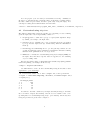
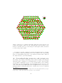


![libsbml[5pt] Developer`s Manual](http://vs1.manualzilla.com/store/data/005677524_1-a4aef53ff9933c16603010582721c07c-150x150.png)