Download Cosmology Population Monte Carlo

Cosmology Population Monte Carlo
CosmoPMC v1.2
Martin Kilbinger
Karim Benabed
Olivier Cappé
Jean Coupon
Jean-François Cardoso
Gersende Fort
Henry J. McCracken
Simon Prunet
Christian P. Robert
Darren Wraith
User’s manual
Contents
1. What is CosmoPMC?
1
1.1. Importance sampling . . . . . . . . . . . . . . . . . . . . . . . . . . . . . . .
1.2. This manual . . . . . . . . . . . . . . . . . . . . . . . . . . . . . . . . . . . .
2. Installing CosmoPMC
2.1.
2.2.
2.3.
2.4.
2
Software requirements . . . . . .
Download and install pmclib . . .
Patch pmclib . . . . . . . . . . . .
Download and install CosmoPMC
.
.
.
.
.
.
.
.
.
.
.
.
.
.
.
.
.
.
.
.
.
.
.
.
.
.
.
.
.
.
.
.
.
.
.
.
.
.
.
.
.
.
.
.
.
.
.
.
.
.
.
.
.
.
.
.
.
.
.
.
.
.
.
.
.
.
.
.
.
.
.
.
.
.
.
.
.
.
.
.
.
.
.
.
.
.
.
.
.
.
.
.
.
.
.
.
3. Running CosmoPMC
2
3
4
4
5
3.1. Quick reference guide . . . . . . . . . . . . . . . . . . . . . . . . . . . . . . .
3.2. CosmoPMC in detail . . . . . . . . . . . . . . . . . . . . . . . . . . . . . . .
3.3. Output files . . . . . . . . . . . . . . . . . . . . . . . . . . . . . . . . . . . .
4. Cosmology
4.1.
4.2.
4.3.
4.4.
4.5.
4.6.
4.7.
4.8.
4.9.
1
2
5
6
8
12
Basic calculations . . . . . . . . . . . . . . . . . . . .
Cosmic shear . . . . . . . . . . . . . . . . . . . . . .
SNIa . . . . . . . . . . . . . . . . . . . . . . . . . . .
CMB anisotropies . . . . . . . . . . . . . . . . . . . .
Galaxy clustering . . . . . . . . . . . . . . . . . . . .
BAO . . . . . . . . . . . . . . . . . . . . . . . . . . .
Redshift distribution . . . . . . . . . . . . . . . . . .
CMB and the power spectrum normalisation parameter
Parameter files . . . . . . . . . . . . . . . . . . . . .
.
.
.
.
.
.
.
.
.
.
.
.
.
.
.
.
.
.
.
.
.
.
.
.
.
.
.
.
.
.
.
.
.
.
.
.
.
.
.
.
.
.
.
.
.
.
.
.
.
.
.
.
.
.
.
.
.
.
.
.
.
.
.
.
.
.
.
.
.
.
.
.
.
.
.
.
.
.
.
.
.
.
.
.
.
.
.
.
.
.
.
.
.
.
.
.
.
.
.
.
.
.
.
.
.
.
.
.
.
.
.
.
.
.
.
.
.
12
14
18
19
20
23
23
24
24
5. The configuration file
24
6. Post-processing and auxiliary programs
35
6.1.
6.2.
6.3.
6.4.
6.5.
6.6.
Plotting and nice printing . . . .
Mean and confidence intervals .
Importance sampling . . . . . .
Bayesian evidence, Bayes’ factor
Reparameterisation . . . . . . .
Analysis . . . . . . . . . . . . .
.
.
.
.
.
.
.
.
.
.
.
.
.
.
.
.
.
.
.
.
.
.
.
.
.
.
.
.
.
.
.
.
.
.
.
.
.
.
.
.
.
.
.
.
.
.
.
.
.
.
.
.
.
.
.
.
.
.
.
.
.
.
.
.
.
.
.
.
.
.
.
.
.
.
.
.
.
.
.
.
.
.
.
.
.
.
.
.
.
.
.
.
.
.
.
.
.
.
.
.
.
.
.
.
.
.
.
.
.
.
.
.
.
.
.
.
.
.
.
.
.
.
.
.
.
.
.
.
.
.
.
.
.
.
.
.
.
.
.
.
.
.
.
.
.
.
.
.
.
.
7. Using and modifying the code
7.1. Modifying the existing code . . . . . . . . . . . . . . . . . . . . . . . . . . .
7.2. Creating a new module . . . . . . . . . . . . . . . . . . . . . . . . . . . . . .
7.3. Error passing system . . . . . . . . . . . . . . . . . . . . . . . . . . . . . . .
36
36
37
37
37
38
39
39
39
41
Acknowledgments
42
PMC references
43
Bibliography
43
A. File formats
46
A.1. Data files . . . . . . . . . . . . . . . . . . . . . . . . . . . . . . . . . . . . .
A.2. Output file names . . . . . . . . . . . . . . . . . . . . . . . . . . . . . . . . .
A.3. Multi-variate Gaussian/Student-t (mvdens), mixture models (mix mvdens) . . .
46
48
48
B. Syntax of all commands
50
C. MCMC
59
C.1.
C.2.
C.3.
C.4.
C.5.
MCMC configuration file . .
Proposal and starting point .
Output files . . . . . . . . .
Diagnostics . . . . . . . . .
Resuming an interrupted run
.
.
.
.
.
.
.
.
.
.
.
.
.
.
.
.
.
.
.
.
.
.
.
.
.
.
.
.
.
.
.
.
.
.
.
.
.
.
.
.
.
.
.
.
.
.
.
.
.
.
.
.
.
.
.
.
.
.
.
.
.
.
.
.
.
.
.
.
.
.
.
.
.
.
.
.
.
.
.
.
.
.
.
.
.
.
.
.
.
.
.
.
.
.
.
.
.
.
.
.
.
.
.
.
.
.
.
.
.
.
.
.
.
.
.
.
.
.
.
.
.
.
.
.
.
.
.
.
.
.
.
.
.
.
.
60
60
61
61
61
1. What is CosmoPMC?
1. What is CosmoPMC?
name
CosmoPMC (Cosmology Population Monte Carlo) is a Bayesian sampling method to explore
the likelihood of various cosmological probes. The sampling engine is implemented with the
package pmclib. It is called Population Monte Carlo (PMC), which is a novel technique to sample
from the posterior (Cappé et al. 2008). PMC is an adaptive importance sampling method which
iteratively improves the proposal to approximate the posterior. This code has been introduced,
tested and applied to various cosmology data sets in Wraith et al. (2009). Results on the Bayesian
evidence using PMC are discussed in Kilbinger et al. (2010).
1.1. Importance sampling
One of the main goals in Bayesian inference is to obtain integrals of the form
Z
π( f ) =
f (x)π(x)dx
(1)
over the posterior distribution π which depends on the p-dimensional parameter x, where f is
an arbitrary function with finite expectation under π. Of interest are for example the parameter
mean ( f = id) or confidence regions S with f = 1S being the indicator function of S . The
Bayesian evidence E, used in model comparison techniques, is obtained by setting f = 1, but
instead of π using the unnormalised posterior π0 = L · P in (1), with L being the likelihood and
P the prior.
The evaluation of (1) is challenging because the posterior is in general not available analytically,
and the parameter space can be high-dimensional. Monte-Carlo methods to approximate the
above integrals consist in providing a sample {xn }n=1...N under π, and approximating (1) by the
estimator
N
1 X
π̂( f ) =
f (xn ).
(2)
N n=1
Markov Chain Monte Carlo (MCMC) produces a Markov chain of points for which π is the
limiting distribution. The popular and widely-used package cosmomc (http://cosmologist.
info/cosmomc; Lewis & Bridle 2002) implements MCMC exploration of the cosmological
parameter space.
Importance sampling on the other hand uses the identity
Z
Z
π(x)
π( f ) =
f (x)π(x)dx =
f (x)
q(x) dx
q(x)
1
(3)
2. Installing CosmoPMC
where q is any probability density function with support including the support of π. A sample
{xn } under q is then used to obtain the estimator
N
1 X
π̂( f ) =
f (xn ) wn ;
N n=1
wn =
π(xn )
.
q(xn )
(4)
The function q is called the proposal or importance function, the quantities wn are the importance
weights. Population Monte Carlo (PMC) produces a sequence qt of importance functions (t =
1 . . . T ) to approximate the posterior π. Details of this algorithm are discussed in Wraith et al.
(2009).
The package CosmoPMC provides a C-code for sampling and exploring the cosmological parameter space using Population Monte Carlo. The code uses MPI to parallelize the calculation
of the likelihood function. There is very little overhead and on a massive cluster the reduction in wall-clock time can be enormous. Included in the package are post-processing, plotting
and various other analysis scripts and programs. It also provides a Markov Chain Monte-Carlo
sampler.
1.2. This manual
This manual describes the code CosmoPMC, and can be obtained from www.cosmopmc.info.
CosmoPMC is the cosmology interface to the Population Monte Carlo (PMC) engine pmclib.
Documentation on the PMC library can be found at the same url. The cosmology module of
CosmoPMC can be used as stand-alone program, it has the name nicaea (http://www2.iap.
fr/users/kilbinge/nicaea).
Warning: Use undocumented features of the code at your own risk!
2. Installing CosmoPMC
2.1. Software requirements
CosmoPMC has been developed on GNU/Linux and Darwin/FreeBSD systems and should run
on those architectures. Required are:
• C-compiler (e.g. gcc, icc)
• pmclib (Sect. 2.2)
• GSL (http://www.gnu.org/software/gsl), version 1.15 or higher
• FFTW (http://www.fftw.org)
• Message Parsing Interface (MPI) (http://www-unix.mcs.anl.gov/mpi) for parallel
calculations
2
2. Installing CosmoPMC
Optional:
• csh, for post-processing, auxiliary scripts; recommended
• perl (http://www.perl.org), for post-processing, auxiliary scripts; recommended
• yorick (http://yorick.sourceforge.net), post-processing, mainly plotting
• python (http://www.python.org), for running the configuration script
• R (http://www.r-project.org), post-processing
To produce 1D and 2D marginal posterior plots with scripts that come with CosmoPMC, either
yorick or R are required.
Necessary for CMB anisotropies support:
• Fortran compiler (e.g. ifort)
• Intel Math Kernel libraries (http://software.intel.com/en-us/intel-mkl)
• CAMB (http://camb.info,http://cosmologist.info/cosmomc)
• WMAP data and likelihood code (http://lambda.gsfc.nasa.gov)
2.2. Download and install pmclib
The package pmclib can be downloaded from the CosmoPMC site http://www.cosmopmc.
info.
After downloading, unpack the gzipped tar archive
> tar xzf pmclib x.y.tar.gz
This creates the pmclib root directory pmclib x.y. pmclib uses waf1 instead of configure/make
to compile and build the software. Change to that directory and type
> ./waf --local configure
See ./waf --help for options. The packages lua, hdf5 and lapack are optionally linked with
pmclib but are not necessary to run CosmoPMC. Corresponding warnings of missing files can be
ignored. Instead of a local installation (indicated by --local), a install prefix can be specified
with --prefix=PREFIX (default /usr/local).
1
http://code.google.com/p/waf
3
2. Installing CosmoPMC
2.3. Patch pmclib
For CosmoPMC v1.2 and pmclib v1.x, a patch of the latter is necessary. From http://www.
cosmopmc.info , download patch pmclib 1.x 1.2.tar.gz and follow the instructions in
the readme file readme patch pmclib 1.x 1.2.txt.
2.4. Download and install CosmoPMC
The newest version of CosmoPMC can be downloaded from the site http://www.cosmopmc.
info.
First, unpack the gzipped tar archive
> tar xzf CosmoPMC v1.2.tar.gz
This creates the the CosmoPMC root directory CosmoPMC v1.2. Change to that directory and
run
> [python] ./configure.py
This (poor man’s) configure script copies the file Makefile.no host to Makefile.host and
sets host-specific variables and flags as given by the command-line arguments. For a complete
list, see ‘configure.py --help’.
Alternatively, you can copy by hand the file Makefile.no host to Makefile.host and edit
it. If the flags in this file are not sufficient to successfully compile the code, you can add more
flags by rerunning configure.py, or by manually editing Makefile.main. Note that a flag in
Makefile.main is overwritten if the same flag is present in Makefile.host.
To compile the code, run
> make; make clean
On success, symbolic links to the binary executables (in ./exec) will be set in ./bin.
It is convenient to define the environment variable COSMOPMC and to set it to the main CosmoPMC
directory. For example, in the C-shell:
> setenv COSMOPMC /path/to/CosmoPMC v1.2
This command can be placed into the startup file (e.g. ˜/.cshrc for the C-shell). One can also
add $COSMOPMC/bin to the PATH environment variable.
4
3. Running CosmoPMC
3. Running CosmoPMC
3.1. Quick reference guide
Examples
To get familiar with CosmoPMC, use the examples which are contained in the package. Simply
change to one of the subdirectories in $COSMOPMC/Demo/MC Demo and proceed on to the point
Run below.
User-defined runs
To run different likelihood combinations, or your own data, the following two steps are necessary
to set up a CosmoPMC run.
1. Data and parameter files
Create new directory with newdir pmc.sh. When asked, enter the likelihood/data type.
More than one type can be chosen by adding the corresponding (bit-coded) type id’s.
Symbolic links to corresponding files in $COSMOPMC/data are set, and parameter files
from $COSMOPMC/par files are copied to the new directory on request.
If necessary, copy different or additional data and/or parameter files to the present directory.
2. Configuration file
Create the PMC configuration file config pmc. Examples for existing data modules can
be found in $COSMOPMC/Demo/MC Demo, see also Sect. 5 for details.
In some cases, information about the galaxy redshift distribution(s) have to be provided,
and the corresponding files copied (see $COSMOPMC/Demo for example files ‘nofz*’).
Run
Type
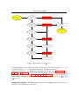
> $COSMOPMC/bin/cosmo pmc.pl -n NCPU
to run CosmoPMC on NCPU CPUs. See ‘cosmo pmc.pl -h’ for more options. Depending on
the type of initial proposal (Sect. 3.2), a maximum-search is started followed by a Fisher matrix
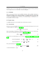
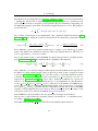
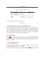
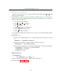
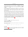
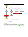
calculation. After that, PMC is started. Fig. 1 shows a flow chart of the script’s actions.
5
3. Running CosmoPMC
Diagnostics
Check the files perplexity and enc. If the perplexity reaches values of 0.8 or larger, and if the
effective number of components (ENC) is not smaller than 1.5, the posterior has very likely been
explored sufficiently. Those and other files are updated during run-time and can be monitored
while PMC is running. See Sect. 3.3.1 for more details.
Results
The text file iter {niter-1}/mean contains mean and confidence levels. The file
iter {niter-1}/all contour2d.pdf shows the 1d- and 2d-marginals. Plots can be redone
or refined, or created from other than the last iteration with plot contour2d.pl. Note that in
the default setting, the posterior plots are not smoothed. See Sect. 6.1.1for more details, and for
information on the alternative script plot confidence.R.
3.2. CosmoPMC in detail
This section describes in more detail how PMC is run, and which decisions the user has to make
before starting and after stopping a PMC run.
The choice of the initial proposal, used during the first PMC iteration, is of
great importance for a successful PMC run. The following options are implemented, determined
by the key ‘sinitial’ in the configuration file (see Sect. 5):
Initial proposal
1. sinitial = fisher rshift The Fisher matrix is used as the covariance of a multivariate Gaussian/Student-t distribution g. A mixture-model is constructed by creating D
copies of g. Each copy is displaced from the ML point by a random uniform shift, and its
variance is stretched by random uniform factor.
2. sinitial = fisher eigen A mixture-model is constructed in a similar way as the first
case, with the difference that the shift from the ML point is now performed along the
major axes of the Fisher ellipsoid. Note that if the Fisher matrix is diagonal, the shift of
each component only concerns one parameter.
3. sinitial = file The initial proposal is read from a file (of mix mvdens format), e.g.
from a previous PMC run.
4. sinitial = random pos Mixture-model components with random variance (up to half
the box size) and random positions. This case should only be used if the posterior is
suspected to be multi-modal, or the calculation of the Fisher matrix fails.
In many cases, a mixture of multi-variate Gaussians as the proposal is the best choice. For that,
set the degrees-of-freedom (ν) parameter df to -1. For a posterior with heavy tails, a Student-t
6
3. Running CosmoPMC
cosmo_pmc.pl
start
pmcsim_*
exist?
yes
run PMC (preprocess)
no
Fisher matrix
needed?
no
run PMC (full)
plot results
yes
fisher
exists?
cosmo_pmc.pl
end
yes
no
config_fish
exists?
yes
run go_fishing
no
maxlogP
exists?
yes
create config_fish
no
config_max
exists?
yes
run max_post
no
create config_max
Figure 1: Flow chart for cosmo pmc.pl.
distribution might be more suited. The degrees of freedom ν can be chosen freely; ν = 3 is a
common choice. For ν → ∞, a Gaussian distribution is reached asymptotically.
If the Fisher matrix has to be calculated for the initial proposal, the script cosmo pmc.pl calls
max post and go fishing to estimate the maximum-likelihood point and the Hessian at that
point, respectively. The script config pmc to max and fish.pl can be used to create the
corresponding configuration files from the PMC config file for manual calls of max post and
go fishing.
The PMC algorithm automatically updates the proposal after each
iteration, no user interference is necessary.
Updating the proposal
7
3. Running CosmoPMC
The method to update the proposal is a variant of the Expectation-Maximization algorithm (EM,
Dempster et al. 1977). It leads to an increase of the perplexity and an increase of ESS. Detailed
descriptions of this algorithm in the case of multi-variate Gaussian and Student-t distributions
can be found in Cappé et al. (2008) and Wraith et al. (2009).
A component can ‘die’ during the updating if the number of points sampled from that component is less than MINCOUNT = 20, or its weight is smaller than the inverse
total number of sample points 1/N. There are two possibilities to proceed. First, the component
is ‘buried’, its weight set to zero so that no points are sampled from it in subsequent iterations.
Alternatively, the component can be revived. In this case, it is placed near the component φd0
which has maximum weight, and it is given the same covariance as φd0 .
Dead components
The first case is the standard method used in Wraith et al. (2009). The second method tries to
cure cases where the majority of components die. This can happen if they start too far off from
the high-density posterior region. Often, only one component remains to the end, not capable of
sampling the posterior reliably.
Both options can be chosen using the config file (Sect. 5) key sdead comp = {bury|revive}.
If an error occurs during the calculation of the likelihood, the error is intercepted and
the likelihood is set to zero. Thus, the parameter vector for which the error occurs is attributed a
zero importance weight and does not contribute to the final sample. An error message is printed
to stderr (unless CosmoPMC is run with the option -q) and PMC continues with the next point.
Errors
An error can be due to cosmological reasons, e.g. a redshift is probed which is larger than the
maximum redshift in a loitering Universe. Further, a parameter could be outside the range of a
fitting formulae, e.g. a very small scalar spectral index in the dark matter transfer function.
Usually, the errors printed to stderr during PMC sampling can be ignored.
The GSL random number generator is used to generate random variables.
It is initialised with a seed reading the current time, to produce different (pseudo-) random
numbers at each call. The seed is written to the log file. Using the option ’-s SEED’, a userspecified seed can be defined. This is helpful if a run is to be repeated with identical results.
Random numbers
3.3. Output files
Each iteration i produces a number of output files which are stored in subdirectories iter i of
the CosmoPMC starting directory. Files which are not specific to a single iteration are placed in
the starting directory.
8
3. Running CosmoPMC
3.3.1. Diagnostics
Unlike in MCMC, with adaptive importance sampling one does not have to worry about convergence. In principle, the updating process can be stopped at any time. There are however
diagnostics to indicate the quality and effectiveness of the sampling.
Perplexity and effective sample size
perplexity
The perplexity p is defined in eq. (18) of Wraith et al. (2009). The range of p is [0; 1], and
will approach unity if the proposal and posterior distribution are close together, as measured by
the Kullback-Leibler divergence. The initial perplexity is typically very low (< 0.1) and should
increase from iteration to iteration. Final values of 0.99 and larger are not uncommon, but also
for p of about 0.6-0.8 very accurate results can be obtained. If p is smaller than say 0.1, the
PMC sample is most likely not representative of the posterior. Intermediate values for p are not
straight-forward to interpret.
Closely related to the perplexity is the effective sample size ESS, which lies in the range [1; N].
It is interpreted as the number of sample point with zero weight (Liu & Chen 1995). A large
perplexity is usually accompanied by a high ESS. For a successful PMC run, ESS is much higher
than the acceptance rate of a Monte Carlo Markov chain, which is typically between 0.15 and
0.25.
The file perplexity contains the iteration i, perplexity p, ESS for that iteration, and the total
ESS. This file is updated after each iteration and can therefore be used to monitor a PMC run.
If there are points with very large weights, they can dominate the other points whose normalised
weights will be small. Even a few sample points might dominate the sum over weights and result
in a low perplexity. The perplexity is the most sensitive quantity to those high-weight points,
much more than e.g. the mean, the confidence intervals or the evidence.
Effective number of proposal components
enc
The proposal qt provides useful information about the performance of a PMC run. For example,
the effective number of components, defined in complete analogy to ESS,
−1
 D
X n o2 
t

ENC = 
αd  ,
(5)
d=1
is an indication of components with non-zero weight. If ENC is close to unity, the number of
remaining components to sample the posterior is likely to be too small to provide a representative sample. For a badly chosen initial proposal, this usually happens already at the first few
iterations. By monitoring the file enc which is updated each iteration, an unsuccessful PMC run
can be aborted.
9
3. Running CosmoPMC
The effective number of components can also be determined from any proposal file (mix mvdens
format) with the script neff proposal.pl.
An additional diagnostic is the evolution of the proposal components with iteration. This illustrates whether the components spread out nicely across the high-posterior region and reach
a more or less stationary behaviour, or whether they stay too concentrated at one point. The
scripts proposal mean.pl (proposal var.pl) read in the proposal information qt and plot
the means (variances) as function of iteration t.
3.3.2. Results
PMC samples
iter i/pmcsim
This file contains the sample points. The first column is the (unnormalised) importance weight
(log), the second column denotes the component number from which the corresponding point
was sampled. Note that the nclip points with highest weights are not considered in subsequent
calculations (of moments, perplexity, evidence etc.). The next p columns are the p-dimensional
parameter vector. Optionally, nded numbers of deduced parameters follow.
Proposals
iter i/proposal
The proposal used for the importance sampling in iteration i is in mix mvdens format (Sect. A.3).
The final proposal, updated from the sample of the last iteration, is proposal fin.
Mean and confidence intervals
iter i/mean
This file contains mean and one-dimensional, left- and right-sided confidence levels (c.l.). A
c.l. of p% is calculated by integrating the one dimensional normalised marginal posterior starting
from the mean in positive or negative direction, until a density of p%/2 is reached. PMC outputs
c.l.’s for p = 63.27%, 95.45% and 99.73%. With the program cl one sided, one-sided c.l.’s
can be obtained.
For post-processing, the program meanvar sample outputs the same information (mean and
c.l.) from an existing PMC sample, including possible deduced parameters.
Resampled PMC simulations
iter {niter-1}/sample
If cosmo pmc.pl has been run with the option -p, the directory of the final iteration contains the
file of parameter vectors sample, which is resampled from the PMC simulation pmcsim, taking
into account the importance weights. The resampled points all have unit weight. Resampling is
a post-processing steop, it is performed by calling the R script sample from pmcsimu.R from
cosmo pmc.pl; this can also be done manually with any pmscim simulation.
10
3. Running CosmoPMC
Histograms
iter i/chi j, iter i/chi j k
One- and two-dimensional histograms are written at each iteration to the text files chi j and
chi j k, respectively, where j and k, j < k, are parameter indices. Those histograms can be
used to create 1d- and 2d-marginals, using the script plot contour2d.pl. The bin number is
set by the config entry nbinhist.
In post-processing, use histograms sample to produce histograms from a PMC sample. This
can be useful if deduced parameters have been added to the sample.
Covariance
iter i/covar*.fin
The parameter covariance and inverse covariance are printed to the files covar.fin and, respectively, covarinv.fin. The addition “+ded” in the file name indicates the inclusion of deduced
parameters. The covariance matrices are in “mvdens”-format (see Sect. A.3).
Evidence
evidence
This file contains the Bayesian evidence as a function of iteration. Before the first iteration,
the Laplace approximation using the Fisher matrix is printed to evidence fisher if the file
fisher exists. At each iteration i, iter i/evidence covarinv contains the Laplace approximation of the evidence from the inverse covariance matrix of the sample iter i/pmcsim.
3.3.3. Deduced parameters
Deduced parameters can be part of a PMC simulation. These parameters are not sampling parameters, but they are deduced from the main parameters. For example, if Ωm and ΩΛ are
sampling parameters of a non-flat model, the curvature ΩK = Ωm + ΩΛ can be a deduced parameter.
In most cases, deduced parameters are ignored while running CosmoPMC. They are usually
added to the PMC simulation after the sampling, for example using a script. In the case of
galaxy clustering, add deduced halomodel adds deduced parameters which depend on the
sampling parameters but also on the underlying cosmology and halo model.
A PMC simulation with deduced parameters added can be used as input to histograms sample,
to create the histogram files, now including the deduced parameters. These can then in turn be
read by and plot contour2d.pl to produce 1d- and 2d-marginals, including the deduced parameters. Alternatively, the PMC simulation with added parameters can be resampled using
sample from pmcsimu.R, from which plots can be created by plot confidence.R.
11
4. Cosmology
3.3.4. Other files
Maximum-posterior parameter
max logP
max post stores its estimate of the maximum posterior in this file.
Fisher matrix
fisher
The final result of go fishing, the Fisher matrix in mvdens (Sect. A.3) format.
Log files
log max post, log fish, log pmc
max post, go fishing and cosmo pmc each produce their corresponding log file.
4. Cosmology
The cosmology part of CosmoPMC is essentially the same as the stand-alone package nicaea2 .
This excludes the external program camb and the WMAP likelihood library, which are called by
CosmoPMC for CMB anisotropies. Further, CosmoPMC contains a wrapper layer to communicate between the PMC sampling and the cosmology modules.
4.1. Basic calculations
A number of routines to calculate cosmological quantities are included in the code. These are
• Background cosmology: Hubble parameter, distances, geometry
• Linear perturbations: growth factor, transfer function, cluster mass function, linear 3D
power spectra
• Non-linear evolution: fitting formulae for non-linear power spectra (Peacock & Dodds
1996; Smith et al. 2003), emulators (Heitmann et al. 2009, 2010; Lawrence et al. 2010),
halo model
• Galaxy clustering: HOD model
• Cosmic shear: convergence power spectrum, second-order correlation functions and derived second-order quantities, third-order aperture mass skewness
• CMB anisotropies via camb.
2
http://www2.iap.fr/users/kilbinge/nicaea
12
4. Cosmology
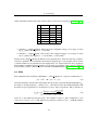
Table 1: Extrapolation of the power spectra
snonlinear
linear
pd96
smith03, smith03 de
coyote10
kmax
333.6 h Mpc−1
333.6 h Mpc−1
333.6 h Mpc−1
2.416 Mpc−1
next
ns − 4
−2.5
Eq. (61), Smith et al. (2003)
no extrapolation
4.1.1. Density parameters
Both the density parameters (ΩX = ρX /ρc ) and the physical density parameters (ωx = Ωx h2 ) are
valid input parameters for sampling with PMC. Internally, the code uses non-physical density
parameters (ΩX ). All following rules hold equivalently for both classes of parameters. Note that
physical and non-physical density parameters can not be mixed, e.g. Ωc and ωK on input causes
the program to abort.
The parameter for massive neutrinos, Ων,mass , is not contained in the matter density Ωm = Ωc +
Ωb .
A parameter which is missing from the input list is assigned the default value, found in the
corresponding cosmology parameter file (cosmo.par), unless there is an inconsistency with
other input parameters. E.g., if Ωde and ΩK are input parameters, Ωm is assigned the value
Ωm = 1 − Ωde − ΩK − Ων,mass , to keep the curvature consistent with ΩK .
A flat Universe is assumed, unless (a) both Ωm and Ωde , or (b) ΩK are given as input parameter.
4.1.2. Matter power spectrum
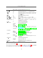
Usually, models of the non-linear power spectrum have a limited validity range in k and/or
redshift. For small k, each model falls back to the linear power spectrum, which goes as Pδ (k) ∝
kns . For large k, the extrapolation as a power law Pδ (k) ∝ next is indicated in Table 4.1.2.
See for more details on the models.
In the coyote10 case, the power spectrum is zero for k > kmax . The
same is true for redshifts larger than the maximum of zmax = 1. See Eifler (2011) for an alternative approach.
The Coyote emulator
The Hubble constant h can not be treated as a free parameter. For a given cosmology, it has to be
fixed to match the CMB first-peak constraint `A = πdls /rs = 302.4, where dls is the distance to
last scattering, and rs is the sound horizon. This can be done with the function set H0 Coyote,
see Demo/lensingdemo.c for an example. When doing sampling with non-physical density
13
4. Cosmology
parameters, h has to be set at each sample point. Alternatively, the physical density parameters
can be sampled, where h is set internally to match the CMB peak.
4.1.3. Likelihood
Each cosmological probe has its own log-likelihood function. The log-likelihood function is
called from a wrapping routine, which is the interface to the PMC sampler. In general, within
this function the model vector is computed using the corresponding cosmology routine. The
exception are the WMAP-modules where the C` ’s are calculated using camb and handed over to
the log-likelihood function as input.
4.2. Cosmic shear
CosmoPMC implements second- and third-order weak lensing observables.
4.2.1. Second-order
The basic second-order quantities in real space for weak gravitational lensing are the two-point
correlation functions ξ± (2PCF) (e.g Kaiser 1992),
Z ∞
1
ξ± (θ) =
d` `Pκ (`)J0,4 (`θ).
(6)
2π 0
Data corresponding to both functions (slensdata=xipm) as well as only one of them (xip,
xim) can be used. The aperture-mass dispersion (Schneider et al. 1998)
Z ∞
1
2
hMap
i(θ) =
d` `Pκ (`)Û 2 (θ`)
(7)
2π 0
is supported for two filter functions Uθ (ϑ) = u(ϑ/θ)/θ2 (Schneider et al. 1998; Crittenden et al.
2002),
!
9
2 1
2
(8)
polynomial (map2poly): u(x) = (1 − x ) − x H(1 − x);
π
3
!
1
x 2 − x2
Gaussian (map2gauss): u(x) =
1−
e 2.
(9)
2π
2
The top-hat shear dispersion (Kaiser 1992)
1
h|γ| iE,B (θ) =
2π
∞
Z
d` ` Pκ (`)
2
0
is used with slensdata = gsqr.
14
4J1 (`θ)
(`θ)2
(10)
4. Cosmology
Pure E-/B-mode separating functions (Schneider & Kilbinger 2007) are chosen with slensdata
= decomp eb. For the lack of analytical expressions for filter functions to obtain these realspace statistics from the convergence power spectrum, they are calculated by integrating over
the 2PCF. The integral is performed over the finite angular interval [ϑmin ; ϑmax ]. The prediction
for the E-mode is
Z
1 ϑmax
E=
dϑ ϑ T + (ϑ) ξ+ (ϑ) ± T − (ϑ) ξ− (ϑ) .
(11)
2 ϑmin
Two variants of filter functions are implemented: The ‘optimized’ E-/B-mode function Fu &
Kilbinger (2010) for which the real-space filter functions are Chebyshev polynomials of the
second kind,
T + (ϑ) = T̃ +
! N−1
X
2ϑ − ϑmax − ϑmin
x=
=
an Un (x);
ϑmax − ϑmin
n=0
Un (x) =
sin[(n + 1) arccos x]
.
sin(arccos x)
(12)
The coefficients an have been optimized with respect to signal-to-noise and the Ωm -σ8 Fisher
matrix. The function E is defined as a function of the lower angular limit ϑmin . The ratio η of
lower to upper limit, η = ϑmin /ϑmax is fixed.
The second variant are the so-called COSEBIs (Complete Orthogonal Sets of E-/B-mode Integrals; Schneider et al. 2010). We implement their ‘logarithmic’ filter functions,
log
T +,n (ϑ)
=
log
t+,n
"
z = ln
ϑ
ϑmin
!#
= Nn
n+1
X
j=0
cn j z = Nn
j
n+1
Y
(z − rn j )..
(13)
j=1
The coefficients cn j are fixed by integral conditions that assure the E-/B-mode decomposition of
the 2PCF on a finite angular integral. They are given by a linear system of equations, which
is given in Schneider et al. (2010). To solve this system, a very high numerical accuracy
is needed. The Mathematica notebook file $COSMOPMC/par files/COSEBIs/cosebi.nb,
adapted from Schneider et al. (2010), can be run to obtain the coefficients for a given ϑmin
and ϑmax . An output text file is created with the zeros rni and amplitudes Nn . The file name is
cosebi tplog rN [Nmax] [thmin] [thmax], where Nmax is the number of COSEBI modes,
thmin and thmax are the minimum and maximum angular scale ϑmin and ϑmax , respectively.
For a given ϑmin and ϑmax , specified with the config entries th min and th max, CosmoPMC
reads the corresponding text file from a directory that is specified by path. A sample of files
with various scales are provided in $COSMOPMC/par files/COSEBIs.
The COSEBIs are discrete numbers, they are specified by an integer mode number n.
In both cases of pure E-/B-mode separating statistics, the function T − is calculated from T +
according to Schneider et al. (2002).
The additional flag decomp eb filter decides between different filter functions:
15
4. Cosmology
decomp eb filter
FK10 SN
FK10 FoM eta10
FK10 FoM eta50
COSEBIs log
Reference
Fu & Kilbinger (2010)
Fu & Kilbinger (2010)
Fu & Kilbinger (2010)
Schneider et al. (2010)
Filter function typ
optimized Signal-to-noise
optimized Fisher matrix
optimized Fisher matrix
logarithmic
η
1/50
1/10
1/50
The convergence power spectrum Pκ with covariance matrix can be used with the flag slensdata
= pkappa.
4.2.2. Third-order
We implement the aperture-mass skewness (Pen et al. 2003; Jarvis et al. 2004; Schneider et al.
2005) with the Gaussian filter (eq. ??). There are two cases:
• slensdata = map3gauss
D
3 i θ , θ , θ ) (Schneider et al. 2005) with three filter scales.
The ‘generalised’ skewness Map
1 2 3
• slensdata = map3gauss diag
D
3 i θ) using a single aperture filter scale.
The ‘diagonal’ skewness Map
TODO: equations
4.2.3. Second- plus third-order
A joint data vector of second- and third-order observables can be used in CosmoPMC. The
covariance is interpreted as a joint block matrix, with the second-order and third-order autocovariances on the diagonal, and the cross-correlation on the off-diagonal blocks. The possible
scenarios are:
• slensdata = map2gauss map3gauss
Gaussian aperture-mass dispersion and generalised skewness.
• slensdata = map2gauss map3gauss diag
Gaussian aperture-mass dispersion and diagonal skewness.
• slensdata = decomp eb map3gauss
Log-COSEBIs and generalised aperture-mass skewness. The flag decomp eb filter has
to be set to COSEBIs log.
• slensdata = decomp eb map3gauss diag
Log-COSEBIs and diagonal aperture-mass skewness. The flag decomp eb filter has to
be set to COSEBIs log.
16
4. Cosmology
The first two cases use the same filter for second- and third-order, and provide therefore a consistent measure for both orders. The last two cases use the optimal E-/B-mode function known
for second order.
4.2.4. Covariance
The covariance matrix is read from a file, and the inverse is calculated in CosmoPMC. The matrix
has to be positive definite. An Anderson-Hartlap debiasing factor is multiplied to the inverse
(Anderson 2003; Hartlap et al. 2007), which is specified with the config entry corr invcov.This
can also be used to rescale the covariance, e.g. to take into account a different survey area. Set
this value to unity if no correction is desired.
The covariance is either taken to be constant and not dependent on cosmology. In that case,
set scov scaling to cov const. Or the approximated schemes from Eifler et al. (2009) are
adopted, see Kilbinger et al. (2012) for the implementation. In that scheme, the shot-noise
term D is constant, the mixed term M is modulated with Ωm and σ8 using fitting formluae,
and the cosmic-variance term V is proportional to the square of the shear correlation function.
This scheme is available for slensdata = xipm. The three covariance terms have to be read
individually. The entry covname, which for scov scaling = cov const corresponds to the
total covariance matrix, now specified the file name of cosmic-variance term, covname M the
name of the mixed term, and covname D the name of the shot-noise term.
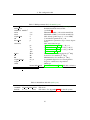
4.2.5. Reduced shear
The fact that not the shear γ but the reduced shear g = γ/(1−κ) is observable leads to corrections
to the shear power spectrum of a few percent, mainly on small scales. These corrections are
either ignored, or modelled to first order according to Kilbinger (2010). This is controlled in
the lensing parameter file (cosmo lens.par). The parameter range where the reduced-shear
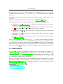
corrections are valid are indicated in Table 2.
4.2.6. Angular scales
The flag sformat describes the mapping of angular scales (given in the data file) and ‘effective’
scales, where the model predictions of the shear functions are evaluated:
1. sformat = angle center: The effective scale is the same as given in the data file,
θeff = θ.
2. sformat = angle mean: The model is averaged over a range of scales [θ0 , θ1 ] given in
the data file.
17
4. Cosmology
Table 2: Parameter limits where the reduced-shear corrections are valid (from Kilbinger 2010).
α
Parameter
lower
upper
1
2
3
4
5
6
7
Ωm
Ωde
w
Ωb
h
σ8
ns
0.22
0.33
-1.6
0.005
0.61
0.65
0.86
0.35
1.03
-0.6
0.085
1.11
0.93
1.16
3. sformat = angle wlinear: The model is the weighted average over a range of scales
[θ0 , θ1 ], where the weight is w = θ/arcmin.
4. sformat = angle wquadr: The model is the weighted average over a range of scales
[θ0 , θ1 ], where the weight is w = a1 (θ/arcmin) + a2 (θ/arcmin)2 .
The first mode (angle center) should be used for aperture-mass, shear rms and ‘ring’ statistics,
since those quantities are not binned, but instead are integrals up to some angular scale θ. For the
correlation functions, in particular for wide angular bins, one of the last three modes is preferred.
The quadratic weighting (angle wquadr) corresponds to a weighting of the correlation function
by the number of pairs3 . This mode was used in the COSMOS analysis (Schrabback et al. 2010).
4.3. SNIa
The standard distance modulus (schi2mode = chi2 simple) for a supernova with index i is
µB,i = m∗B,i − M̄ + α(si − 1) − βci .
(14)
where the quantities measured from the light-curve fit are the rest-frame B-band magnitude m∗B,i ,
the shape or stretch parameter si , and the color ci . The universal absolute SNIa magnitude is M̄,
the linear response parameters to stretch and color are α and β, respectively. The χ2 -function is
h
i2
i , p)
X µB,i ( p) − 5 log10 dL10(zpc
,
(15)
χ2sn (p) =
σ2 (µB,i ) + σ2pv,i + σ2int
i
where dL is the luminosity distance and zi the redshift of object i. The contributions to the
total error for object i are: (1) The light-curve parameter variance σ2 (µB,i ) = θ2t W2 θ2 with the
3
P. Simon, private communication
18
4. Cosmology
parameter vector θ2 = (1, α, β) and the covariance W2 of the data vector (m∗B,i , si , ci ). (2) The
peculiar velocity uncertainty σpv,i = 5/ ln 10 · vp /(c zi ). (3) The intrinsic absolute magnitude
scatter σint .
The Hubble parameter is absorbed into the absolute magnitude which we define as M = M̄ −
5 log10 h70 .
The form of this log-likelihood function has been used in Astier et al. (2006).
The following variations of the distance modulus and log-likelihood are implemented:
• schi2mode = chi2 Theta1: The χ2 is extended to include photometric zero-point uncertainties, see Kilbinger et al. (2009).
• schi2mode = chi2 Theta2 denom fixed: The parameters α and β in the denominator
of (15) are fixed and kept constant during the Monte-Carlo sampling.
• schi2mode = chi2 no sc: The stretch and color parameters are ignored, the distance
modulus is µB,i = m∗B,i − M̄.
• schi2mode = chi2 betaz: Instead of a single parameter, the color response is redshiftdependent, β → β + βz zi .
• chi2 dust: Intergalactic dust absorption is taken into account in the distance modulus,
see Ménard et al. (2010).
The covariance matrix W2 of the data vector (m∗B,i , si , ci ) depends on the parameters α and β. In
a Bayesian framework, this leads to an additional term 21 log det W2 in the log-likelihood function. Taking into account this parameter-dependent term leads however to a biased maximumlikelihood estimator, in particular for α and β4 . Therefore, it is recommended to not include this
term. Use the flag add logdetCov = 0/1 in the configuration file to disable/enable this term.
4.4. CMB anisotropies
The full CMB anisotropies are handled externally: The C` ’s are calculated by calling camb5
(Lewis et al. 2000), the WMAP likelihood function (3rd -, 5th - and 7th -year) is computed using
the WMAP public code6 (Dunkley et al. 2009). The maximum ` up to which the C` ’s are
calculated and used in the likelihood can be determined in the configuration file. An `max = 2000
is recommended for high precision calculations.
The power spectrum from the Sunyaev-Zel’dovich (SZ) effect can be added to the C` ’s, multiplied with an amplitude A as free parameter. The predicted SZ power spectrum is taken from
Komatsu & Seljak (2002). This model has been used in the 3-, 5- and 7-year analyses of the
WMAP data (Komatsu et al. 2011).
4
J. Guy, private communication
http://camb.info
6
http://lambda.gsfc.nasa.gov
5
19
4. Cosmology
Alternatively, the WMAP distance priors (Komatsu et al. 2009) can be employed.
4.5. Galaxy clustering
4.5.1. Halomodel and HOD
The theoretical model of galaxy clustering is the one used in Coupon et al. (2012); see this paper
for details of the model and further references.
As the basis to describe galaxy clustering, we implement the halo-model as reviewed in (Cooray
& Sheth 2002), which accounts for the clustering of dark-matter halos. On top of that, a halo
occupation distribution (HOD) function (Berlind & Weinberg 2002; Kravtsov et al. 2004; Zheng
et al. 2005) is the prescription of how galaxies populate those halos. This function is the number
of galaxies N in a halo of mass M. With the flag hod = berwein02 excl, this number is
expressed as the sum of central (Nc ) plus satellite (Ns ) galaxies,
N(M) = Nc (M) × [1 + Ns (M)] ,
(16)
with
"
!#
log10 M − log10 Mmin
1
nc (M) =
1 + erf
;
2
σlog M
 α

0

; if M > M0
 M−M
M1
,
ns (M) = 

 0
else
(17)
(18)
We further compute the galaxy two-point correlation function ξ(r) and its angular projection
w(θ) using the redshift distribution provided by the user, as well as the galaxy number density
(for a full description of the model see Coupon et al. 2012). To prevent haloes from overlapping,
we implement the halo exclusion formalism as described in Tinker et al. (2005).
For the halo bias, three options are available:
• shalo bias = bias sc
Bias expansion from the spherical collapse model, see e.g. eq. (68) from Cooray & Sheth
(2002).
• shalo bias = bias tinker05
Bias calibrated with numerical simulations, Tinker et al. (2005) eq. (A1).
• shalo bias = bias tinker10
Updated bias fitting formua from Tinker et al. (2010), eq. (6) and Table 2.
The mass function describes the number of halos for a given mass and redshift. It is defined as
ρ ν f (ν) dν
dn
= 0
,
d ln M
M ν d ln M
20
(19)
4. Cosmology
where ν(M, z) = δc (z)/[D+ (z)σ(M)] is a measure of the overdensity with σ(M) being the rms
matter fluctuation in a top-hat window containing the mass M. ρ0 = Ωm ρc,0 is the mean density
of matter at the present day.
The following mass functions are implemented, via the flag smassfct:
• From the spherical/eliptical collapse model:
r
ν f (ν) = A
!
i
2 h
aν2
2 −p
,
1 + (aν ) exp −
2
πaν2
(20)
– ps: p = 0, q = 1 (Press & Schechter 1974)
– st: p = 0.3, q = 0.75 (Sheth & Tormen 1999)
– st2: p = 0.3, q = 0.707 (Sheth & Tormen 1999)
• From numerical simulations:
h
i
ν f (ν) = f (σ) = 0.315 exp −| ln(σ−1 + 0.61|3.8
(21)
– j01: (Jenkins et al. 2001)
The dark-matter halos have the density profile
h
i−1
ρ(r) = ρs (r/rs )α (1 + r/rs )3−α .
(22)
For slopes unequal to the Navarro et al. (1997) value of α = 1, closed expressions for the Fourier
transform of ρ do not exist, and the code will be slower.
The concentration parameter is given by
"
#−β
M
c0
c(M, z) =
,
1 + z M?
(23)
following Takada & Jain (2003). The parameters c0 and β can be chosen freely in the halomodel
parameter file halomodel.par.
The log-likelihood function is the sum of the contribution from the angular correlation function
and the galaxy number density ngal :
h
i2
Xh
nobs
− nmodel
i
h
i
gal
gal
χ2 =
wobs (θi ) − wmodel (θi ) C −1 wobs (θ j ) − wmodel (θ j ) +
,
(24)
ij
σ2ngal
i, j
where nmodel
is estimated at the mean redshift of the sample.
gal
The number of galaxies (second term in eq. 24) can be included in the following way, with the
config flag sngal fit type:
21
4. Cosmology
• ngal lin fit: linear (standard; according to the above equation)
• ngal log fit: logarithmical
• ngal no fit: no inclusion, second term is omitted
• ngal lin fit only: exclusive, first term is omitted
4.5.2. Deduced parameters
The following deduced parameters can be computed:
• Mean galaxy bias
bg (z) =
Z
dM bh (M, z) n(M, z)
N(M)
,
ngal (z)
(25)
where bh is the halo bias, and
ngal (z) =
Z
N(M) n(M, z) dM
(26)
is the total number of galaxies.
• Mean halo mass
hMhalo i(z) =
Z
dM M n(M, z)
N(M)
.
ngal (z)
(27)
• Fraction of satellite galaxies
fs (z) = 1 − fc (z);
fc (z) =
Z
dM n(M, z)
Nc (M)
.
ngal (z)
(28)
Use the program add deduced halomodel to add those deduced parameters to a PMC sample.
See the example config file config pmc ded in Demo/MC Demo/HOD/CFHTLS-T06.
4.5.3. Clustering data
The angular two-point correlation function w(θ) is implemented, with the flag shalodata =
woftheta. The measured (input) data wmes is corrected for the integral constraint, via
w(θ) = wmes (θ) + wC ,
assuming that the measured correlation function can be fit by a power law
wmes (θ) ≈ Aw θ−δ − C .
(29)
(30)
The program haloplot outputs the correlation functions w(θ) and ξ(r), the HOD function N(M),
and deduced parameters for given HOD input parameters.
22
4. Cosmology
4.5.4. Comoving volume
The comoving volume is needed to calculate the comoving number density of galaxies, following from the halomodel and the HOD parameters. There are two possibilities to calculate the
comoving volume VC . First, if zmin and zmax are larger than zero in the HOD parameter file
halomodel.par (see Table 7), VC is computed between those two redshifts. Second, if both
numbers are < 0, VC is weighted by the redshift distribution n(z), see e.g. eq. (28) in Ross &
Brunner (2009). In this weighting, the maximum value of n(z) is set to unity.
4.6. BAO
BAO constraints are implemented with two distance measures:
• smethod = distance A
The distance parameter A is defined in Eisenstein et al. (2005) as
√
DV (z) Ωm
A(z) =
c/H0 z
where
"
DV (z) =
fK2 [w(z)]
cz
H(z)
(31)
#1/3
(32)
is the spherically averaged distance to redshift z.
• smethod = distance d z
The distance parameter d is the ratio of sound horizon rs at drag epoch zd to spherically
averaged distance (e.g. Percival et al. 2007),
d(z) =
rs (zd )
.
DV (z)
(33)
We use the fitting formula for the drag redshift zd from Eisenstein & Hu (1998) and calculate the sound horizon as the distance a sound wave can travel prior to zd by numerical
integration.
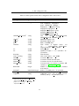
4.7. Redshift distribution
Some of the cosmology modules require a redshift distribution, for example lensing and HOD.
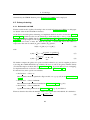
Table 3 lists the implemented redshift distributions n(z), via the flag nofz.
Each redshift bin can have a different type. The syntax for a redshift bin file is described in
Appendix A.1.5.
23
5. The configuration file
Table 3: Redshift distribution types
nofz
Description
hist
single
ludo
jonben
ymmk
Histogram
Single redshift
Fitting function
n(z) ∝ . . .
Pn−1
i=0 Ni · 1[zi ;zi+1 ]
δD (z − z0 ) h
i
(z/z0 )α exp − (z/z0 )β
za / zb + c
za + zab / zb + c
parameter list
(see text)
z0 , z0
zmin , zmax , α, β, z0
zmin , zmax , a, b, c
zmin , zmax , a, b, c
All redshift distributions are internally normalised as
Z zmax
dz n(z) = 1.
(34)
zmin
4.8. CMB and the power spectrum normalisation parameter
The power spectrum normalisation parameter taken as input for camb is ∆2R , which is the amplitude of curvature perturbations at the pivot scale k0 = 0.002 Mpc−1 . For lower-redshift probes
such as lensing or HOD, the normalisation is described by σ8 , the rms fluctuation of matter in
spheres of 8 Mpc/h. To combine those probes in a PMC run, ∆2R has to be an input parameter,
and σ8 a deduced parameter. CMB has to come first in the list of data sets so that camb can
calculate σ8 , which in turn is handed over to the lensing likelihood.
4.9. Parameter files
Tables 4 - 6 list the contents of the parameter files for basic cosmology, lensing, SNIa and HOD.
Proto-types can be found in $COSMOPMC/par files. These files specify the default values of
parameters and flags. These default values are over-written if any of those parameter is used for
Monte-Carlo sampling.
5. The configuration file
The programs max post, go fishing, cosmo pmc, and cosmo mcmc read a configuration file
on startup. Each configuration file consist of two parts:
The first, basic part is common to all four config file types (Table 9). It consists of (1) the
parameter section, (2) the data section and (3) the prior section. The data-specific entries in the
24
5. The configuration file
Table 4: Basic cosmology parameter file (cosmo.par)
Omega m
Omega de
w0 de
w1 de
Ωm
Ωde
w0
w1
h 100
Omega b
Omega nu mass
N eff nu mass
h
Ωb
Ων,mass
Neff,ν,mass
normalization
σ8
n spec
snonlinear
ns
linear
pd96
smith03
smith03 de
coyote10
stransfer
bbks
eisenhu
eisenhu osc
sgrowth
heath
growth de
sde param
jassal
linder
normmode
a min
amin
Matter density, cold dark matter + baryons
Dark-energy density (if w = −1, corresponds to ΩΛ
Dark-energy equation-of-state parameter (constant term)
Dark-energy equation-of-state parameter (linear term,
see sde param)
Dimensionless Hubble parameter
Baryon density
Massive-neutrino density (so far only for CMB)
Effective number of massive neutrinos (so far only for
CMB)
Power-spectrum normalisation at small scales (for
normmode==0, see below)
Scalar power-spectrum index
Power spectrum prescription
Linear power spectrum
Peacock & Dodds (1996)
Smith et al. (2003)
Smith et al. (2003) + dark-energy correction from
icosmo.org
‘Coyote Universe’, Heitmann et al. (2009), Heitmann
et al. (2010), Lawrence et al. (2010)
Transfer function
Bardeen et al. (1986)
Eisenstein & Hu (1998) ‘shape fit’
Eisenstein & Hu (1998) with BAO wiggles
Linear growth factor
Heath (1977) fitting formula
Numerical integration of differential equation for δ (recommended)
Dark-energy parameterisation
w(a) = w0 + w1 a(1 − a)
w(a) = w0 + w1 (1 − a)
Normalization mode. 0: normalization=σ8
Minimum scale factor
data section are listed in Table 11.
The second part is type-specific. See Table 10 for the PMC part, and Table 13 for the MCMC
part. Example files can be found in subdirectories of $COSMOPMC/Demo/MC DEMO.
25
5. The configuration file
Table 5: Weak lensing parameter file (cosmo lens.par)
cosmo file
nofz file
redshift modulea
stomo
tomo all
tomo auto only
tomo cross only
sreduced
none
K10
q
q mag sizeb
a
b
Basic cosmology file name (cosmo.par)
Redshift distribution master file
(see Table 8)
Tomography correlations
All correlations
Only auto-correlations (ii)
Only cross-correlations (i , j)
Reduced-shear treatment
No correction
Fitting-formulae from Kilbinger (2010)
Magnification-bias coefficient, q = 2(α + β − 1)
(see Kilbinger 2010, eq. 16)
only if nofz file = "-"
only if sreduced = K10
Table 6: SNIa parameter file (cosmo SN.par)
cosmo file
Theta2
−M α − β βz
Basic cosmology file name (cosmo.par)
Distance modulus parameters
26
5. The configuration file
Table 7: HOD parameter file (halomodel.par)
cosmo file
nofz file
redshift modulea
zmin
zmax
alpha NFW
c0
beta NFW
zmin
zmax
α
c0
β
smassfct
M min
M1
M0
sigma log M
alpha
shod
ps
st
st2
j01
Mmin
M1
M0
σlog M
α
berwein02 hexcl
a
Basic cosmology file name (cosmo.par)
Redshift distribution master file
(see Table 8)
Minimum redshift (-1 if read from nzfile)
Maximum redshift (-1 if read from nzfile)
Halo density profile slope (α = 1 for NFW)
Concentration parameter at z = 0
Concentration parameter slope of mass dependence
Halo mass function type
(Press & Schechter 1974), p = 0, q = 1
(Sheth & Tormen 1999), p = 0.3, q = 0.75
(Sheth & Tormen 1999), p = 0.3, q = 0.707
(Jenkins et al. 2001)
Minimal mass for central galaxies [h−1 M ]
Scale mass for satellites [h−1 M ]
Minimum mass for satellites [h−1 M ]
Logarithmic dispersion for central galaxies
Slope for satellite mass dependence
HOD type
Berlind & Weinberg (2002) with halo exclusion
only if nofz file = "-"
Table 8: Redshift module file (nofz.par)
Nzbin
snzmode
nzfile
Nz
nz read from files
f1 , f2 , . . ., fNzbin
Number of redshift bins
File mode
File names. See Appendix A.1.5 for the file syntax.
27
5. The configuration file
To create a config file of type max post or go fishing from a PMC config file, the script
config pmc to max and fish.pl can be used.
Some flags are handled internally as integers (enumerations), but identified and set in the config
file with strings. The corresponding key word carries the same name as the internal variable,
preceded with an ‘s’, e.g. the integer/string pair lensdata/slensdata.
The prior file, indicated if desired with the flag sprior, is a file in mvdens format. It specifies
a Gaussian prior with mean and covariance as given in the file. Note that the covariance and not
the inverse covariance is expected in the file.
28
5. The configuration file
Table 9: Basic, common part of the configuration file
version
double
npar
n ded
integer
integer
spar
string
min
max
npar+n
npar+n
Config file version. Upwards compatibility (config file
version > CosmoPMC version) cannot be guaranteed.
Downwards compatibility (config file version < CosmoPMC version) is most likely ensured.
Parameter section
Number of parameters
Number of deduced parameters. The deduced parameters are not sampled but deduced from the other parameters and written to the output files as well
Parameterisation type, necessary for the wrapping into
the individual posterior parameters and for plotting, see
Table 12 for possible parameters
ded doubles Parameter minima
ded doubles Parameter maxima
ndata
sdata
integer
string
Data section
Number of data sets
Data set 1
..
.
sdata
string
Data set ndata
sprior
[nprior
string
integer
[indprior
npar × {0, 1}
Prior section
Prior file name (“-” for no prior)
If sprior , “-”: Number of parameters to which prior
applies]
If sprior , “-”: Indicator flags for prior parameters]
29
5. The configuration file
Table 10: PMC part of the configuration file
nsample
niter
fsfinal
niter
nclipw
integer
integer
integer
integer
integer
Sample size per iteration
Number of iterations
Sample size of final iteration is fsfinal × nsample
Number of iterations (importance runs)
The nclipw points with the largest weights are discarded
df
double
ncomp
sdead comp
sinitial
integer
string
string
fshifta
double
fvara
prop ini nameb
fminc
double
string
double
Proposal section
Degrees of freedom (df=-1 is Gaussian, df=3 is ‘typical’
Student-t)
Number of components
One of ‘bury’, ‘revive’
Proposal type (one of fisher rshift, fisher eigen,
file, random position)
Random shift from ML point ∼ U(−r, r);
r = fshift/(max-min)
Random multiplier of Fisher matrix
File name of initial proposal
Components have variance ∼ U(fmin, (max − min)/2)
integer
Histogram section
Number of density histogram bins
nbinhist
a
only if sinitial = fisher rshift or fisher eigen
only if sinitial = file
c
only if sinitial = random position
b
30
5. The configuration file
Table 11: Data-specific entries in the configuration file’s data section
Weak gravitational lensing Lensing
slensdata
string
sdecomp eb filtera
string
th minb
th maxb
pathb
sformat
double
double
double
string
a1c
a2c
double
double
datname
scov scaling
covname
covname Md
covname Dd
corr invcov
string
string
string
string
string
double
Nexclude
integer
excludee
model file
sspecial
Nexclude integers
string
string
a
only if slensdata = decomp eb
only if sdecom eb filter = COSEBIs log
c
only if sformat = angle wquadr
d
only if scov scaling = cov ESH09
e
only if Nexclude > 0
b
31
Data
type,
one
of
xipm, xip,
xim, map2poly, map2gauss,
gsqr, decomp eb, pkappa,
map3gauss, map3gauss diag,
map2gauss map3gauss,
map2gauss map3gauss diag,
decomp eb map3gauss,
decomp eb map3gauss diag
One
of
FK10 SN, FK10 FoM eta10,
FK10 FoM eta50, COSEBIs log
Minimum angular scale
Maximum angular scale
Path to COSEBIs files
Data format of angular scales, one
of
angle center, angle mean,
angle wlinear, angle wquadr
Linear weight
Quadratic weight, w = a1 · θ/arcmin + a2 ·
(θ/arcmin)2
Data file name
One of cov const, cov ESH09
Covariance file name
Covariance mixed term file name
Covariance shot-noise term file name
Correction factor for inverse covariance ML
estimate, see Hartlap et al. (2007)
Number of redshift bin pairs to be excluded
from analysis
Indices of redshift pairs to be excluded
Parameter file name, e.g. cosmo lens
Additional prior, one of none (recommended), unity, de conservative
5. The configuration file
Supernovae type Ia SNIa
datname
string
datformat
string
schi2mode
string
Theta2 denoma
zAV nameb
datname beta db
add logdetCov
2 doubles
string
string
integer
model file
sspecial
string
string
a
b
Data file name
Data format, SNLS firstyear
χ2 and distance modulus estimator type (one
of
chi2 simple, chi2 Theta2 denom fixed,
chi2 betaz, chi2 dust, chi2 residual)
Fixed α, β in χ2 -denominator
File with AV (z) table
Prior file (mvdens format) on βd (“-” if none)
1 if 0.5 log det Cov is to be added to log-likelihood, 0 if not
(recommended; see Sect. 4.3)
Parameter file name, e.g. cosmo SN
Additional prior, one of none (recommended), unity,
de conservative
only if schi2mode = chi2 Theta2 denom fixed
only if schi2mode = chi2 dust
Table 11: Data-specific entries in the configuration file’s data section (continued).
CMB anisotropies CMB
scamb path string
/path/to/scamb
data path
string
/path/to/wmap-data. This path should contain the directory data with subdirectories healpix data, highl, lowlP,
lowlP
Cl SZ file string
File with SZ correction angular power spectrum (“-” if none)
lmax
integer Maximum ` for angular power spectrum
accurate
0|1
Accurate reionisation and polarisation calculations in camb
model file string
Parameter file name, e.g. cosmoDP.par
sspecial
string
Additional prior, one of none (recommended), unity,
de conservative
WMAP distance priors CMBDistPrior
datname
string Data (ML point and inverse covariance) file
model file string Parameter file name, e.g. cosmo lens.par
sspecial
string Additional prior, one of none (recommended),
de conservative
32
unity,
5. The configuration file
Galaxy clustering (HOD) GalCorr
shalodata
string
Data type, woftheta
shalomode
string
χ2 type, one of galcorr var, galcorr cov, galcorr log
datname
string
Data (+variance) file name
a
covname
string
Covariance file name
corr invcov
double Correction factor for inverse covariance ML estimate, see Hartlap et al. (2007)
delta
double Power-law slope δ, for integral constraint
intconst
double Integral constant C
area
double Area [deg2 ]
sngal fit type string
Likelihood type, inclusion of galaxy number.
One
of
ngal lin fit, ngal log fit, ngal no fit,
ngal lin fit only
ngalb
double Number of observed galaxies
ngalerrb
double Error on the number of observed galaxies
model file
string
Parameter file name
sspecial
string
Not used for HOD, set to none
a
b
only if shalomode = galcorr cov, galcorr log
not if sngal fit type = ngal no fit
Table 11: Data-specific entries in the configuration file’s data section (continued).
Baryonic acoustic oscillations BAO
smethod
string BAO method, one of distance A, distance d z
datname
string Data + covariance file name (mvdens format)
model file string Parameter file name, e.g. cosmoDP.par
sspecial
string Additional prior, one of none (recommended),
de conservative
unity,
Table 12 contains a list of input parameters, which can be given as strings to the spar key in the
config file.
33
5. The configuration file
Table 12: Input parameters
Name
Symbol
Basic cosmology
Omega m
omega m
Omega b
omega b
100 omega b
Omega de
omega de
Omega nu mass
omega nu mass
Omega c
omega c
Omega K
omega K
w0 de
w1 de
(some of them given in cosmo.par)
Ωm
Matter density, cold dark matter + baryons
ωm
Ωb
Baryon density
ωb
100 × ωb
Ωde
Dark-energy density (if w = −1, corresponds to ΩΛ
ωde
Ων,mass
Massive-neutrino density (so far only for CMB)
ων,mass
Ωc
Cold dark matter
ωc
ΩK
Curvature density parameter
ωK
w0
Dark-energy equation-of-state parameter (constant term)
w1
Dark-energy equation-of-state parameter (linear term, see
sde param)
h
Dimensionless Hubble parameter
Neff,ν,mass Effective number of massive neutrinos (so far only for CMB)
σ8
Power-spectrum normalisation at small scales
2
∆R
Power-spectrum normalization at large scales (CMB)
ns
Scalar power-spectrum index
αs
Running spectral index (so far only for CMB)
nt
Tensor power-spectrum index
r
Tensor to scalar ratio
ln r
τ
Optical depth for reionisation
ASZ
SZ-power spectrum amplitude
h 100
N eff nu mass
sigma 8
Delta 2 R
n spec
alpha s
nt
r
ln r
tau
A SZ
Description
34
6. Post-processing and auxiliary programs
Table 12: Input parameters (continued)
SNIa-specific (some of them given in cosmo SN.par)
M
M − log10 h70 Universal SNIa magnitude
alpha α
Linear response factor to stretch
beta
β
Linear response factor to color
beta z βz
Redshift-dependent linear response to color
beta d βd
Linear response to the color component due to intergalactic dust
Galaxy-clustering-specific (some of them given in halomodel.par)
M min
Mmin
Minimum halo mass for central galaxies
[M h−1 ]
−1
log10 M min
log10 Mmin /(M h )
M1
M1
Scale mass for satellite galaxies [M h−1 ]
−1
log10 M 1
log10 [M1 /(M h )]
M0
M0
Minimum halo mass for satellite galaxies
[M h−1 ]
−1
log10 M 0
log10 M0 /(M h )
sigma log M
σlog M
Dispersion for central galaxies
alpha halo
αh
Slope of satellite occupation distribution
M halo av∗
hMh i
Average halo mass [M h−1 ]
log10 M halo av∗ log10 hMh /(M h−1 )i
hbh i
Average halo bias
b halo av∗
N gal av∗
hNg i
Average galaxy number per halo
∗
fr sat
fs
Fraction of satellite galaxies to total
ngal den∗
ng
Comoving galaxy number density [Mpc−3 h3 ]
log10 ng
log10ngal den∗
6. Post-processing and auxiliary programs
All scripts described in this section are located in $COSMOPMC/bin.
35
6. Post-processing and auxiliary programs
6.1. Plotting and nice printing
6.1.1. Posterior marginal plots
Marginals in 1d and 2d can be plotted in two ways, using (1) plot contour2d.pl or (2)
plot confidence.R. The first is a perl script calling yorick for plotting, the second is an
R script. The second option produces nicer plots in general, in particular, smoothing workes
better without producing over-smoothed contours. Further, filled contours with more than one
data set are only possible with the R option, yorick can only combine several plots with empty
contours. The computation time of the R script is however much longer.
1. plot contour2d.pl creates 1d and 2d marginals of the posterior, from the histogram
files chi2 j and chi2 j k.
To smooth 1d and 2d posteriors with a Gaussian, use plot contour2d.pl -n -g
FACTOR. The width of the Gaussian is equal to the box size divided by FACTOR. It is recommended to test the smoothing width FACTOR by setting it to a negative number which
causes both smoothed and unsmoothed curves being plotted. This can reveal cases of
over-smoothing. If contours have very different width in different dimension, the addition
option -C uses the PMC sample covariance (from the file covar+ded.fin) as the covariance for the Gaussian. For the final plot, replace -FACTOR with FACTOR to remove the
unsmoothed curves. Remove the option -n to add color shades to the 2d contours.
The file log plot contains the last plot command with all options. This can be used to
reproduce and modify a plot which has been generated automatically by other scripts, e.g.
cosmo pmc.pl.
2. plot confidence.R creates 1d and 2d marginals of the posterior, from the re-sample file
sample.
Smoothing is done with a kernel density estimation using the R function kde2d. The
kernel width can be set with the option -g. The number of grid points, relevant both for
smoothing and filled contours, is set with -N. Use both -i and -j options to only plot the
2D marginals of parameters iandj to save computation time.
6.2. Mean and confidence intervals
From a “mean” output file, containing parameter means and confidence levels, one can create a
ps/pdf file using the command mean2eps.pl.
This is equivalent to the following steps (see also essential cosmo pmc run.pl):
• meanvar2tab.pl creates a table with parameter names and values formatted in TEXformat.
• tab2tex.pl wraps a LATEX table header around the table.
36
6. Post-processing and auxiliary programs
• txt2tex.pl wraps a LATEX header around the file.
Example:
> meanvar2tab.pl -s 1 -p 2 -e iter 9/mean > mean.tab
> tab2tex.pl -s 1.25 mean.tab > mean in.tex
> txt2tex.pl mean in.tex > mean.tex
6.2.1. PMC proposal
proposal mean.pl (proposal var.pl) creates plots of the proposal component’s means (variances) as function of the iteration.
6.3. Importance sampling
A PMC simulation file (pmcsim) from an earlier PMC run, corresponding to a sample from
posterior p1 , can be used to do importance sampling with another posterior p2 . For that, simply
replace the data section of the earlier config file with the corresponding data section of posterior
p2 . The command importance sample creates a new PMC simulation which corresponds to a
sample under the posterior product p1 · p2 .
6.4. Bayesian evidence, Bayes’ factor
evidence.pl calculates and prints the evidence from a PMC simulation file. The same information is printed to the file evidence during a PMC run.
bayes factor.pl prints Bayes’ factor between two PMC runs together with the Jeffrey scale.
evidence list.pl prints a list of evidences for a number of PMC runs.
6.5. Reparameterisation
remap.sh swaps and removes parameters from a MCMC or PMC run. The histogram files,
mean and covariances are remapped. This is useful if different runs are to be reduced to a
common parameter set for comparison or joint plotting. The removal of parameters is equivalent
to marginalisation over the corresponding parameter subspace.
For example, suppose there is a SNIa run in directory Sn, and a lensing run in Lensing. SNIa
has the following parameters:
Omegam Omegade w0de M alpha beta
37
6. Post-processing and auxiliary programs
Lensing has the parameters:
Omegam sigma8 w0de Omegade h100
In Sn, create the file remap.dat with the line
0 1 2
In Lensing, create the file remap.dat with the line
0 3 2
In both directories run the command
> remap.sh -i iter <niter-1>
which creates sub-directories remap containing symbolic links and/or copies of histogram files
to/from iter {niter-1}, mean, covariance files and updated configuration files.
To create joint marginal plots, simply run
> plot contours2d.pl -c /path/to/Sn/remap/config pmc -n /path/to/Sn/remap
/path/to/Lensing/remap
New parameters, sampled from a flat or Gaussian distribution, can be added using add par from prior.pl.
6.6. Analysis
6.6.1. mvdens/mix mvdens format utilities
See Sect. A.3 for a description of the mvdens and mix mvdens formats.
fisher to meanvar.pl reads a mvdens file, inverts the covariance matrix and prints the mean
and variance.
corr coeff.sh reads a mvdens or block matrix file and prints the correlation matrix of the
covariance.
diag mvdens.pl replaces the covariance by its diagonal.
add par to mvdens.pl adds parameters to a mvdens file. Useful, if CosmoPMC is run with
additional parameters, and the initial proposal is chosen from a previous run with the reduced
parameter set.
38
7. Using and modifying the code
6.6.2. PMC simulation/MCM chain utilities
sample2fixpar.pl reads a sample file and fixes a parameter by cutting off all points outside a
given (narrow) range.
6.6.3. PMC proposal diagnostics
neff proposal.pl calculates the effective number of components (eq. 5). It is the same quantity which is printed to the file enc.
7. Using and modifying the code
7.1. Modifying the existing code
Note: Code to be used with MPI should not contain global variables and static variables.
7.2. Creating a new module
In this section, the steps required to add a new cosmology module to CosmoPMC are described.
1. Create the directory newmodule and create (or copy) files with the necessary code to
deal with the data and likelihood. Include files (*.h) should be in newmodule/include,
source files (*.c) in newmodule/src. Edit the (or create a new) Makefile (in newmodule)
and add the rules libnewmodule.so, libnewmodule.dylib and libnewmodule.a as
well as the rule clean.
2. In wrappers/include/types.h:
Define a new data type by extending the enumeration data t. Add the corresponding
string (for identification of the module in the configuration file) in the macro sdata t(i),
and increase Ndata t by one.
3. In wrappers/include/all wrappers.h:
Add the line
#include "newmodule.h"
4. In tools/include/par.h:
If necessary, add new parameter types (p newparameter) to enumeration par t, add the
corresponding identifier strings to the macro spar t, and increase Npar t by one.
Optional: Add the parameter name and syntax for different programs (e.g. gnuplot,
yorick, TEX) to bin/spar.txt.
39
7. Using and modifying the code
5. In wrappers/src/wrappers.c:
Add the corresponding case to the ‘switch’ instruction in the function init func t. This
function sets the data type.
6. Create the files wrappers/include/newmodule.h and wrappers/src/newmodule.c.
(Those files need to have different names than the files in newmodule/{src,include}.)
Write the following functions:
a) init function newmodule
b) read from config newmodule
c) init newmodule
d) likeli newmodule (returning log L)
e) special newmodule (optional)
f) print newmodule (optional)
To see what these functions are supposed to do, have a look at already existing modules,
e.g. in bao.c.
7. In Makefile.main:
a) In the section “Additional directories”, define the path to the new module’s directory
as
NEWMODULE = $(COSMOPMC)/newmodule
b) In the section “Libraries”, define the library of the new module as
LIBNEWMODULE = libnewmodule.$(EXT)
c) In the section “Combined cosmo include and linker flags”, add the following flags:
-I$(NEWMODULE)/include to the variable IINCDIRS
-L$(NEWMODULE) to LLIBDIRS
-lnewmodule to LLIBS.
8. In exec/Makefile:
Define the new rule:
$(LIBNEWMODULE):
cd $(NEWMODULE) && $(MAKE) $@
(The second line has to start with a <TAB> and not with spaces.)
9. Optional: Extend newdir pmc.sh.
40
7. Using and modifying the code
7.3. Error passing system
Most of the situations where an error occurs are intercepted by the program. In such a case, a
variable *err of type error* is set via the macros
*err = addError(error_type, "message", *err, __LINE__);
or
*err = addErrorVA(error_type, "formatted message", *err,
__LINE__, VA_LIST);
printing the current line and function in the code, a message and the error type (negative integer).
With
testErrorRet(test, error_type, "message", *err, __LINE__,
return_value);
or
testErrorRetVA(test, error_type, "formatted message", *err,
__LINE__, return_value, VA_LIST);
a conditional error is produced if the (Boolean) expression test is true. The error is transported
up the stack to the calling function with the macro
forwardError(*err, __LINE__, return_value);
Omit return value in case of a void function. This can be used as diagnostics even for errors
deep in the hierarchy of functions.
During the calculation of the importance weights, any error is intercepted and the corresponding
point does not contribute to the final sample. See Sect. 2 for more details. Therefore, in the
routines which calculate the importance weights, the following is used:
forwardErrorNoReturn(*err, __LINE__, return_value);
ParameterErrorVerb(*err, param, quiet, ndim);
In case of an error, the first line forwards the error but does not return from the current routine. The second line prints the ndim-dimensional parameter param to stderr (if quiet!=1) and
purges the error.
To exit on an error, use
41
7. Using and modifying the code
quitOnError(*err, __LINE__, FILE)
This is usually done only from the main program.
More macros and functions regarding error communication and handling can be found in the
files errorlist.h, errorlist.c which are part of pmclib.
Acknowledgements
CosmoPMC was developed with support of the CNRS ANR ECOSSTAT, contract number ANR05-BLAN-0283- 04 ANR ECOSSTAT.
We thank P. Astier, F. Beaujean, J. Guy, L. Fu, A. Halkola, J. Hartlap, B. Joachimi, J. Lui, K.
Markovič, P. Schneider, F. Simpson, R. E. Smith, M. Takada and I. Tereno for discussions and
insights which helped to develop the cosmology code.
We thank L. Fu for helping with and testing the lensing E-/B-mode decomposition and the thirdorder lensing code.
We acknowledge R. .E. Smith and J. A. Peacock for making public their code halofit7 , which
we implemented into CosmoPMC.
The people from the Coyote project8 are thanked for making their code public. An adapted
version of their emulator is part of this code.
The following people are thanked for providing data or simulations:
M. Kowalski for the Union data (Kowalski et al. 2008), J. Hartlap and S. Hilbert for the Lensing
covariance, computed using ray-tracing through the Millennium Simulation (Schrabback et al.
2010).
7
8
http://www.roe.ac.uk/˜jap/haloes
http://www.lanl.gov/projects/cosmology/CosmicEmu
42
7. Using and modifying the code
PMC references
Introductory papers on PMC
Cappé et al. (2004)
Population Monte Carlo
Cappé et al. (2008)
Adaptive importance sampling in general mixture classes
Comparison of sampling methods including PMC
Robert & Wraith (2009)
Computational methods for Bayesian model choice
Main papers on CosmoPMC
Wraith et al. (2009)
Estimation of cosmological parameters using adaptive importance sampling
Kilbinger et al. (2010)
Bayesian model comparison in cosmology with Population
Monte Carlo
PMC applied to cosmological data
Schrabback et al. (2010)
Evidence of the accelerated expansion of the Universe from
weak lensing tomography with COSMOS
Ménard et al. (2010)
On the impact of intergalactic dust on cosmology with Type Ia
supernovae
Benabed et al. (2009)
TEASING: a fast and accurate approximation for the low multipole likelihood of the cosmic microwave background temperature
Coupon et al. (2012)
Galaxy clustering in the CFHTLS-Wide: the changing relationship between galaxies and haloes since z ∼ 1.2?
Kilbinger et al. (2012)
CFHTLenS: Combined probe cosmological model comparison
using 2D weak gravitational lensing
Benjamin et al. (2012)
CFHTLenS tomographic weak lensing: Quantifying accurate
redshift distributions
Simpson et al. (2012)
CFHTLenS: Testing the Laws of Gravity with Tomographic
Weak Lensing and Redshift Space Distortions
Other publications which use PMC
Joachimi & Taylor (2011) Forecasts of non-Gaussian parameter spaces using Box-Cox
transformations
¯ decays: the standard model
Beaujean et al. (2012)
Bayesian fit of exclusive b → s``
operator basis
43
References
References
Anderson, T. W. 2003, An introduction to multivariate statistical analysis, 3rd edn. (WileyInterscience)) 17
Astier, P., Guy, J., Regnault, N., et al. 2006, A&A, 447, 31 19
Bardeen, J. M., Bond, J. R., Kaiser, N., & Szalay, A. S. 1986, ApJ, 304, 15 25
Beaujean, F., Bobeth, C., van Dyk, D., & Wacker, C. 2012, Journal of High Energy Physics, 8,
30 43
Benabed, K., Cardoso, J., Prunet, S., & Hivon, E. 2009, MNRAS, 400, 219 43
Benjamin, J., Van Waerbeke, L., Heymans, C., Kilbinger, M., et al. 2012, submitted to MNRAS,
also arXiv:1212.3327 43
Berlind, A. A. & Weinberg, D. H. 2002, ApJ, 575, 587 20, 27
Cappé, O., Douc, R., Guillin, A., Marin, J.-M., & Robert, C. 2008, Statist. Comput., 18(4), 447
1, 8, 43
Cappé, O., Guillin, A., Marin, J.-M., & Robert, C. 2004, J. Comput. Graph. Statist., 13, 907 43
Cooray, A. & Sheth, R. 2002, Phys. Rep., 372, 1 20
Coupon, J., Kilbinger, M., McCracken, H. J., et al. 2012, A&A, 542, A5 20, 43
Crittenden, R. G., Natarajan, P., Pen, U.-L., & Theuns, T. 2002, ApJ, 568, 20 14
Dempster, A., Laird, N., & Rubin, D. 1977, J. Royal Statist. Society Series B, 39, 1 8
Dunkley, J., Komatsu, E., Nolta, M. R., et al. 2009, ApJS, 180, 306 19, 61
Eifler, T. 2011, MNRAS, 1490 13
Eifler, T., Schneider, P., & Hartlap, J. 2009, A&A, 502, 721 17
Eisenstein, D. J. & Hu, W. 1998, ApJ, 496, 605 23, 25
Eisenstein, D. J., Zehavi, I., Hogg, D. W., et al. 2005, ApJ, 633, 560 23
Fu, L. & Kilbinger, M. 2010, MNRAS, 401, 1264 15, 16
Hartlap, J., Simon, P., & Schneider, P. 2007, A&A, 464, 399 17, 31, 33
Heath, D. J. 1977, MNRAS, 179, 351 25
44
References
Heitmann, K., Higdon, D., White, M., et al. 2009, ApJ, 705, 156 12, 25
Heitmann, K., White, M., Wagner, C., Habib, S., & Higdon, D. 2010, ApJ, 715, 104 12, 25
Jarvis, M., Bernstein, G., & Jain, B. 2004, MNRAS, 352, 338 16
Jenkins, A., Frenk, C. S., White, S. D. M., et al. 2001, MNRAS, 321, 372 21, 27
Joachimi, B. & Taylor, A. N. 2011, ArXiv e-prints 43
Kaiser, N. 1992, ApJ, 388, 272 14
Kilbinger, M. 2010, A&A, 519, A19+ 17, 18, 26
Kilbinger, M., Benabed, K., Guy, J., et al. 2009, A&A, 497, 677 19
Kilbinger, M., Fu, L., Heymans, C., et al. 2012, submitted to MNRAS, also arXiv:1212.3338
17, 43
Kilbinger, M., Wraith, D., Robert, C. P., et al. 2010, MNRAS, 405, 2381 1, 43
Komatsu, E., Dunkley, J., Nolta, M. R., et al. 2009, ApJS, 180, 330 20, 48
Komatsu, E. & Seljak, U. 2002, MNRAS, 336, 1256 19
Komatsu, E., Smith, K. M., Dunkley, J., et al. 2011, ApJS, 192, 18 19
Kowalski, M., Rubin, D., Aldering, G., et al. 2008, ApJ, 686, 749 42
Kravtsov, A. V., Berlind, A. A., Wechsler, R. H., et al. 2004, ApJ, 609, 35 20
Lawrence, E., Heitmann, K., White, M., et al. 2010, ApJ, 713, 1322 12, 25
Lewis, A. & Bridle, S. 2002, Physical Review D, 66, 103511 1
Lewis, A., Challinor, A., & Lasenby, A. 2000, Astrophys. J., 538, 473 19
Liu, J. & Chen, R. 1995, JASA, 90, 567 9
Ménard, B., Kilbinger, M., & Scranton, R. 2010, MNRAS, 406, 1815 19, 43
Navarro, J. F., Frenk, C. S., & White, S. D. M. 1997, ApJ, 490, 493 21
Peacock, J. A. & Dodds, S. J. 1996, MNRAS, 280, L19 12, 25
Pen, U.-L., Zhang, T., Van Waerbeke, L., et al. 2003, ApJ, 592, 664 16
Percival, W. J., Cole, S., Eisenstein, D. J., et al. 2007, MNRAS, 381, 1053 23
45
A. File formats
Press, W. H. & Schechter, P. 1974, ApJ, 187, 425 21, 27
Robert, C. P. & Wraith, D. 2009, in Proceedings of MaxEnt 2009, to be published by American
Institute of Physics, also arXiv:0907.5123 43
Ross, A. J. & Brunner, R. J. 2009, MNRAS, 399, 878 23
Schneider, P., Eifler, T., & Krause, E. 2010, A&A, 520, A116 15, 16
Schneider, P. & Kilbinger, M. 2007, A&A, 462, 841 15
Schneider, P., Kilbinger, M., & Lombardi, M. 2005, A&A, 431, 9 16
Schneider, P., Van Waerbeke, L., Jain, B., & Kruse, G. 1998, MNRAS, 296, 873 14
Schneider, P., Van Waerbeke, L., & Mellier, Y. 2002, A&A, 389, 729 15
Schrabback, T., Hartlap, J., Joachimi, B., et al. 2010, A&A, 516, A63+ 18, 42, 43
Sheth, R. K. & Tormen, G. 1999, MNRAS, 308, 119 21, 27
Simpson, F., Heymans, C., Parkinson, D., et al. 2012, MNRAS accepted, also arXiv:1212.3339
43
Smith, R. E., Peacock, J. A., Jenkins, A., et al. 2003, MNRAS, 341, 1311 12, 13, 25
Takada, M. & Jain, B. 2003, MNRAS, 340, 580 21
Tinker, J. L., Robertson, B. E., Kravtsov, A. V., et al. 2010, ApJ, 724, 878 20
Tinker, J. L., Weinberg, D. H., Zheng, Z., & Zehavi, I. 2005, ApJ, 631, 41 20
Wraith, D., Kilbinger, M., Benabed, K., et al. 2009, Phys. Rev. D, 80, 023507 1, 2, 8, 9, 43, 59
Zheng, Z., Berlind, A. A., Weinberg, D. H., et al. 2005, ApJ, 633, 791 20
A. File formats
A.1. Data files
A.1.1. Lensing
For all lensdata t types, the data format is the same. Each line contains the data for a given
angular scale and (arbitrary many) redshift bin pair combinations.
46
A. File formats
The angular scales are defined as follows. For lensformat = angle center, the fist column
contains the angular bin center in arc minutes. For the cases lensformat = angle mean,
angle wlinear and angle wquadr, first two columns specify the lower and upper end of the
angular bin.
Following the angular information are the data. For Nz redshift bins, Nz (Nz + 1)/2 columns specify all pair combinations (i j)i≤ j in lexical order, that is (11)(12)(13) . . . (1Nz )(22)(23) . . . (Nz Nz ).
Note that for lensdata = xipm the first Nθ lines of the data file contain ξ+ for Nθ angular
scales, the last Nθ lines contain ξ− , where the angular scales (first or first two columns) are
identical in both halfs.
The covariance matrix is in block format: It consists of N lines and N columns, where N =
Ns Nz (Nz + 1)/2 is the length of the data. Usually, Ns is the number of measured angular scales,
Nθ , unless there is more than one data point per scale (e.g. for lensdata = xipm, Ns = 2Nθ ).
A matrix element Ci j equals hdi d j i − hdi ihd j i, where di is the ith data point. In the counting
over angular scale and redshift, the former varies faster than the latter9 . For example, with two
redshift bins and three angular scales, the element C77 is the data variance for the redshift pair
(11) and angular scale θ1 (starting counting at zero). Or, in other words, the covariance matrix
consists of Nz (Nz + 1)/2 block sub-matrices, each of size Ns × Ns . Each sub-matrix corresponds
to one redshift bin combination. It is therefore easy to exclude some redshift bins, by (1) setting
the diagonal of a sub-matrix to a very high value, and (2) setting the off-diagonal to zero (see
the Nexclude parameter in the config file, Table 11).
A.1.2. SNIa
The SNIa data file in SN SALT format starts with the following two lines:
@INTRINSIC_DISPERSION double
@PECULIAR_VELOCITY double
The peculiar velocity value is in units of km/s. This is followed by a list of supernovae, one
object on each line as follows:
name z m s c < m2 > < s2 > < c2 > < ms > < mc > < sc >
A.1.3. BAO
The BAO distance measures are modeled as Gaussian variables, the data files are in mvdens
format (see Sect. A.3). In the same file, following the mvdens data, there is a list of redshifts,
corresponding to where the distances are measured.
9
This was wrongly stated here until version 1.01.
47
A. File formats
A.1.4. CMB
The CMB data for WMAP are the ones released by the WMAP team. They are not included in
CosmoPMC and can be obtained e.g. from the LΛMBDΛ site10 .
The SZ correction power spectrum file has two columns in each row containing ` and C` , respectively. The first line has to start with ` = 2.
The CMB distance priors (Komatsu et al. 2009) are given in mvdens format.
A.1.5. Redshift distribution
The first line of a file describing a the redshift distribution for a redshift bin contains the type,
see Sect. 4.7,
# nofz
This is followed by the list of parameter values, in the order given in Table 3. Each parameter
value has to be in a new line, with the exeption of the histogram, nofz = single. In that case,
the parameter lines are as follows:
z0
z1
···
zn−1
zn
N0
N1
Nn−1
0
Ni is the number of galaxies in the bin [zi ; zi+1 ]. The last line denotes the upper limit of the last
histogram bin zn = zmax , followed by a zero. For nofz = single, the file has to contain two
identical lines with the value of z0 in each line.
A.2. Output file names
The default names of all output files are defined in stdnames.h. Edit this file and to make
clean; make to set user-defined file names. Note however that some of the pre-processing
scripts expect the default names.
A.3. Multi-variate Gaussian/Student-t (mvdens), mixture models (mix mvdens)
The mvdens file format is as follows. The first (header) line contains four integers:
10
http://lambda.gsfc.nasa.gov
48
A. File formats
p
ν
B
c.
Here, p is the number of dimensions, ν the degrees of freedom. For a multi-variate Gaussian,
choose ν = −1, and ν > 0 for Student-t. B indicates the number of secondary diagonal of the
covariance matrix which are updated during the PMC iterations. For most purposes, B can be
set equal to p, which corresponds to the whole matrix being updated. Finally, c is 1 if the matrix
is Cholesky-decomposed and 0 otherwise.
This is followed by p doubles indicating the mean, followed by p lines with p doubles each,
giving the (symmetric) covariance matrix.
Here is an example of a 5-dimensional multi-variate Gaussian (not Cholesky-decomposed):
5 -1 5 0
0.38559 -1.5238 19.338 1.3692 -2.4358
0.0053677 -0.025608 0.00066748 -0.0011893 0.00087517
-0.025608 0.16837 -0.0079163 0.0027364 -0.0035709
0.00066748 -0.0079163 0.0011077 0.0010986 -0.00067815
-0.0011893 0.0027364 0.0010986 0.016716 0.0026266
0.00087517 -0.0035709 -0.00067815 0.0026266 0.014881
The mix mvdens format has two doubles as the header:
D
p
where D is the number of components of the mixture and ndim the dimension. This is followed
by D blocks specifying the weights wd (doubles) and data md (in mvdens format) of the D
multi-variate densities of the mixtures.
w1
m1
w2
m2
...
wD
mD .
The weights should be normalised,
PD
d=1 wd
= 1.
In many cases, an mvdens file indicates a parameter covariance matrix, for example to be used
as Gaussian prior using the config file flag sprior. In some cases, the inverse covariance matrix
is expected, as in the case of the Fisher matrix.
49
B. Syntax of all commands
B. Syntax of all commands
All following scripts are located in $COSMOPMC/bin. All programs (executables) are located in
$COSMOPMC/exec and linked from $COSMOPMC/bin after running make in $COSMOPMC.
• add deduced halomodel 11, 22
Usage: add_deduced_halomodel [OPTIONS] PSIM [PAR_1 [PAR_2 [...]]]
OPTIONS:
-c CONFIG
Configuration file (default: config_pmc)
-o OUTNAME
Ouput pmcsim name (default: psim+ded)
PSIM
pmc simulation file (pmcsim_iter)
PAR_i
String for deduced parameter #i. If not given, deduced
parameters are read from the config file (default)
• add par from prior.pl 38
Usage: add_par_from_prior.pl [OPTIONS] sample
Adds a new random parameter to a PMC sample file, drawn under a distribution
OPTIONS:
-o OUT
Output sample file OUT (default: ’<sample>.out’
-p DIST
Prior distribution, DIST one of ’Flat’ (default), ’Gauss’
-P ARG
Prior arguments (white-spaced list if more than one). For DIST =
Flat: ARG = ’min max’ (defaut ’-1 1’)
Gauss: ARG = ’mean sigma’
-C COL
Column COL of new parameter (default: last)
-s STR
Name string STR of new parameter
-h
This message
• add par to mvdens.pl 38
add_par_to_mvdens.pl (MIX)MVDENS [OPTIONS]
Adds a parameter to a (mix)mvdens file (e.g. Fisher matrix, PMC proposal)
OPTIONS:
-c COL
Adds parameter in column and row COL (default: last column)
-m VAL
Parameter mean VAL (default 0)
-v VAL
Parameter variance VAL (default 1)
-x
File is in ’mixmvdens’ format
FILE
File name
-h
This message
• bayes factor.pl 37
Usage: bayes_factor.pl [OPTIONS] DIR1 DIR2
Calculates the Bayes factor between models. The corresponding
evidence files (from PMC) have to be in the directories DIR1 and DIR2
OPTIONS:
-i ’ITER1 [ITER2]’ Use iteration ITER1 for DIR1 and ITER2 for DIR2
(default: all iterations)
-f ’EVI1 [EVI2]’
Use files DIR1/EVI1 and DIR2/EVI2 (default: ’evidence’)
-s
Short output, last iteration only
-l
Laplace approx. from Fisher matrix (denoted with iter=-1)
-h
This message
• cl one sided 10
50
B. Syntax of all commands
Usage: cl_one_sided [OPTIONS] sample
OPTIONS:
-c CONFIG
Configuration file (default: config_pmc)
-i INDEX
Parameter index
-d DIR
Direction (DIR=+1,-1)
-v VALUE
Starting value
-w WHICH
WHICH=0: 68%,95%,99.7% c.l. (default)
WHICH=1: 68%,90%,95% c.l.
sample
PMC sample file
The options -i INDEX, -d DIR and -v VALUE are required
• config pmc to max and fish.pl 7, 28
Usage: config_pmc_to_max_and_fish.pl [OPTIONS]
OPTIONS:
-M
Create config file for maximum search (max_post)
-F
Create config file for Fisher matrix (go_fishing)
-c CONFIG
Input PMC config file CONFIG (default: ’config_pmc’)
-r
Random starting point (for maximum search)
-f FID
Fiducial starting point FID. FID is a white-space
separated list in quotes, e.g. ’0.25 0.75’
-p FILE
Fidcucial parameter from FILE (e.g. ’maxlogP’)
-t TOLERANCE Tolerance for maximum-search (default: 0.01)
-d
Calculate only diagonal of Fisher matrix (go_fishing)
-h
This message
One of ’-M’ or ’-F’ is obligatory
The default starting point for maximum search is (max-min)/2
For Fisher matrix (’-F’), a fiducial parameter has to be indicated with ’-f FID’
or ’-p FILE’
• corr coeff.sh 38
Usage: corr_coeff filename [mvdens|block]
• cosmo mcmc
Usage: cosmo_mcmc [OPTIONS]
OPTIONS:
-c CONFIG
Configuration file (default: config_mcmc)
-s SEED
Use SEED for random number generator. If SEED=-1 (default)
the current time is used as seed.
-h
This message
• cosmo pmc 12
Usage: cosmo_pmc [OPTIONS]
OPTIONS:
-c CONFIG
Configuration file (default: ’config_pmc’)
-s SEED
Use SEED for random number generator. If SEED=-1 (default)
the current time is used as seed.
-q
Quiet mode
-h
This message
• cosmo pmc.pl 5, 7, 36
Usage: cosmo_pmc.pl [OPTIONS]
51
B. Syntax of all commands
OPTIONS:
-n NCPU
-c CONFIG
-f FID
-r
-m [c|a]
-d
-D
-a
-s SEED
-S [M|F]
-A [y|n]
-P PATH
-e
-p PRO
-M MULT
-O OPT
-q
-h
Run PMC in parallel on NPCU cpus using ’mpirun’ (default: 1)
Configuration file for PMC (default: config_pmc)
Fiducial starting point FID. FID is a white-space
separated list in quotes, e.g. ’0.25 0.75’
Random starting point for maximum search
(default: (max-min)/2)
Maximum-search method: ’c’ (cg), ’a’ (amoeba)
Calculate only diagonal of Fisher matrix
Do not force Fisher matrix F to be positiv. If F is negative,
script exits with an error
Adaptive numerical differentiation for Fisher matrix
Use SEED for random number generator. If SEED=-1 (default)
the current time is used as seed.
Stops after maximum search (’M’) or Fisher matrix (’F’)
Default answer to all questions on stdin
Use PATH as CosmoPMC directory (default: environment
variable $COSMOPMC)
Create ’essential’ plots
Plotting scripts: ’y’ (yorick; default), ’R’ (R) or ’n’ (none)
Combinations of letters are possible, e.g. ’yR’
Output sample MULT times input (default 1).
Valid if plotting script is ’R’
Pass options OPT to ’plot_contour2d.pl’
Quiet mode
This message
• diag mvdens.pl 38
Usage: diag_mvdens.pl IN
Prints the mvdens file ’IN’ with the covariance replaced by its diagonal.
• essential cosmo pmc run.pl 36
Usage: essential_cosmo_pmc.pl [OPTIONS]
OPTIONS:
-c CONFIG
Uses config file CONFIG (default: ’config_pmc’)
-P PATH
Use PATH as CosmoPMC directory (default: environment
variable $COSMOPMC)
-k
Keep temporary files
-v
Verbose
-h
This message
• evidence.pl 37
Usage: evidence.pl [OPTIONS] SAMPLE
OPTIONS:
-h
This message
SAMPLE
PMC sample file
• evidence list.pl 37
Usage: evidence_list.pl [OPTIONS] DIR1 [DIR2 [...]]
OPTIONS:
-r N
Subtract log(E) from DIRN (default: no subtraction)
52
B. Syntax of all commands
-k KEY
-s SEP
-S SEP
-n
-L
-h
For N=-1 subtract log(E_min)
Use KEY (string list) instead of
directory names (default)
Use SEP as input separator for KEY list
Use SEP as output separator
(default for both: white-space)
Write number of model parameters
Use Laplace approximation (reading file ’evidence_fisher’)
This message
• fisher to meanvar.pl 38
fisher_to_meanvar.pl [OPTIONS] file
OPTIONS:
-n
No inverse
-m
Marginal errors (don’t invert matrix)
-x
mixmvdens format (default: mvdens format)
-k
Keep temporary file ’fishtmp.i’
-h
This message
Options ’-m’ and ’-n’ exclude each other
• get spar.pl
Usage: get_spar.pl [OPTIONS] LANG [PAR1 [PAR2 [...]]]
OPTIONS:
-c CONFIG
Configuration file ONFIG (default ’config_pmc’)
-i INDEX
Returns only par[INDEX]
-P PATH
Use PATH as CosmoPMC directory (default: environment
variable $COSMOPMC)
-p
Print ’p<i> for unknown parameters instead of input string
LANG
One of ’yorick’, ’gnuplot’, ’TeX’, ’R’.
More languages can be defined in spar.txt
PAR1 ...
Prameter strings
• go fishing 7, 12, 12
Usage: go_fishing [OPTIONS]
OPTIONS:
-c CONFIG
Configuration file (default: config_fish)
-a
Adaptive numerical differentiation (default: fixed difference)
-f
Force positive Fisher matrix
-q
Quiet mode
-h
This message
Run in parallel on NP cpu’s: ’mpirun -np NP go_fishing [OPTIONS]
• haloplot 22
Usage: haloplot log10(M_min) log10(M1) log10(M0) sigma_log_M alpha_halo
halomodel.par [OPTIONS]
Outputs HOD-derived quantities
OPTIONS:
-o OUT
Output file name
-t TYPE
Output type, TYPE in [wtheta, wp, xi, xihalo, deltaSig,
nofm, halo, pk], default: wtheta
-nbins
Number of bins
53
B. Syntax of all commands
-range
-z Z
-Mhalo log10M
-c CONFIG
-h
Range (linear scale): min,max
Used fixed redshift Z (no w(theta) output)
log10(Halo mass) for deltaSig and xihalo (in M_sol/h)
PMC config file, to calculate chiˆ2
This message
M_min, M1 and M0 are in units of M_{sol}/h.
• histograms sample 11, 11
Usage: histograms_sample [OPTIONS] sample
OPTIONS:
-c CONFIG
Configuration file (default: config_pmc)
-1
Only 1d histograms
-2
Only 2d histograms
sample
PMC sample file
-h
This message
• importance sample 37
Usage: importance_sample [OPTIONS] INSAMPLE
Performs an importance run on a PMC sample. Run in
parallel with MPI (use mpirun)
OPTIONS:
-c CONFIG
Configuration file (default: config_pmc)
-o OUTSAMPLE
Output sample name (default: ’insample.out’)
-q
Quiet mode
-h
This message
INSAMPLE
Input sample name
• max post 7, 12, 12
Usage: max_post [OPTIONS]
OPTIONS:
-c CONFIG
Configuration file (default: config_max)
-m [c|a|n]
Maximum-search method: ’a’ (amoeba, default), ’c’ (cg),
’n’ (none; print posterior for fiducial parameter and exit)
-t
Test maximum at the end
-s SEED
Use SEED for random number generator. If SEED=-1 (default)
the current time is used as seed.
-p
Prints the maximum-posterior model to the file ’model_maxlog’
-q
Quiet mode
-h
This message
• mean2eps.pl 36
Usage: mean2eps.pl [OPTIONS] MEAN
OPTIONS:
MEAN
File containing mean and confidence levels (output of
’cosmo_pmc’ or ’histograms_sample’
-c CONFIG
Uses config file CONFIG (default: ’config_pmc’)
-P PATH
Use PATH as CosmoPMC directory (default: environment
variable $COSMOPMC)
-o BASE
Outname BASE (default: <MEAN>)
-v
Verbose
54
B. Syntax of all commands
-h
This message
• meanvar2tab.pl 36
Usage: meanvar2tab.pl [OPTIONS] file [file2 [...]]
Options:
-s {123}
-p PREC
-e
-c CONFIG
-t TITLE
-S SEP
-P PATH
-h
68% (1), 95% (2) or 99.7% (3) errors (default = 1)
Output with PREC digits (’%PREC’ format string)
Error(s) written to PREC significant digits (use -p PREC)
Uses config file CONFIG (default: ’config_pmc’)
Title (table heading) TITLE is string list with entries according
to the number of input files
Use SEP as input separator for TITLE list (default: white space)
Use PATH as CosmoPMC directory (default: environment
variable $COSMOPMC)
This message
• meanvar sample 10
Usage: meanvar_sample [OPTIONS] sample
OPTIONS:
-c CONFIG
Configuration file (default: config_pmc)
-w
Ignore weights (default: weights=first column of sample file)
-C
Write covariance and inverse covariance to files
-E
Output evidence
-h
This message
sample
PMC sample file
• neff proposal.pl 10, 39
Usage: neff_proposal.pl PROP
Calculates the effective number of components for the mix_mvdens file ’PROP’
• newdir pmc.sh 5, 40
Usage: newdir_pmc.sh [DIR]
Directory DIR (default: read on input) is created.
Links are set to data files in \$COSMOPMC/data.
Parameter files are copied on request from \$COSMOPMC/par_files.
• plot confidence.R 6, 11, 36
Usage: plot_confidence.R [options]
Options:
-h, --help
Show this help message and exit
-N NGRID, --Ngrid=NGRID
Number of grid points for smoothing (kde2d) (default 100). Use <=30 for
fast-but-dirty plots
-g GSMOOTH, --gsmooth=GSMOOTH
Smoothing kernel width, with respect to box size (default 30). In case of more
55
B. Syntax of all commands
than one sample, use list separated with ’_’ for more than value
-S, --solid
All contours with solid lines
-w WIDTH, --width=WIDTH
Line width (default 1)
-k, --with_keys
Add key to plots
-K KEYSTRING, --keystring=KEYSTRING
Key strings (separate items with ’_’)
-L, --no_key_line
Do not add a line to the keys in the legend
-c CONFIG, --config=CONFIG
Config file (default ’config_pmc’)
-t TITLE, --title=TITLE
Title string for each panel (default empty)
-i INDEX_I, --index_i=INDEX_I
Only create plots with i-th parameter on x-axis
-j INDEX_J, --index_j=INDEX_J
Only create plots with j-th parameter on y-axis
-s SIGMA, --sigma=SIGMA
Plot SIGMA confidence levels (default 3)
-F COLOR_SCHEME, --color_scheme=COLOR_SCHEME
Color scheme (0, 1; default 0)
• plot contour2d.pl 6, 11, 11, 36
Usage: plot_contour2d.pl [OPTIONS] [DIR1 [DIR2 [...]]]
OPTIONS:
-i NITER
-c CONFIG_FILE
-t TITLE
-T TITLE
-n
-w WIDTH
-1 OPT
Number of iterations (needed if do_proposal=2)
Configuration file (default: in order config_mcmc, config_pmc)
Title string for each panel (default empty)
Title string for all_contour2d.{eps|pdf} (default empty)
No shade
Line width WIDTH (default 4)
Add 1d posterior plots. OPT can contain the following letters:
m
Plot line at mean position
123 Plot line at 68%,95%,99.7 density
56
B. Syntax of all commands
t
Write mean and 68% confidence intervals as text
(use with ’m’ and ’1’
n
None of the above
-S
All contours with solid lines
-s N
Outermost level is N sigma
-r
Aspect ratio=1, changes plot limits such that dx=dy
-g FACTOR
Gaussian smoothing of 2d-histograms with variance
box-width/|FACTOR|. If FACTOR is negativ, plots
unsmoothed histogram in addition (use with ’-n’).
Note: For multiple contours, use a list of values "g1 g2 ..."
-G FACTOR
Gaussian smoothing of 1d-histograms (default: 2d factor)
-C
Use covariance (file covar.fin) for Gaussian smoothing
-N NORM
Normalisation of 1d posterior
’m’ Maximum = 1 (default)
’i’ Integral over posterior = 1
-F NUM
Color scheme, NUM=0,1,2
-k
Add key to plots
-K "KEY1 [KEY2 [...]]" Key strings (default: directory names)
-y FS
Font size FS (default 24)
-o FORMAT
Output file format, FORMAT=eps|pdf (default: eps)
-b
Writes the chi2 files in block format
-m PAR
Plots a mark at position PAR (e.g. best-fit). PAR is white-space
separated list (use quotes or ’\ ’, e.g. ’0.3 0.8’)
-P PATH
Use PATH as CosmoPMC root directory (default: environment
variable $COSMOPMC)
-q
Run quietly, no verbose
-h
This message
DIR1 ...
List of directories containing histogram files (chi2_*_*)
Default: DIR1 = ’.’
• proposal mean.pl 10, 37
Usage: proposal_mean.pl [OPTIONS]
OPTIONS:
-d DIR
Directory DIR containing the sub-directories ’iter_*’
with the proposal files (default ’.’)
-c CONFIG
Configuration file CONFIG (default ’DIR/config_pmc’)
-n
No plotting, only creates ’.gnu’ file
-i
x- and y-axes inverted
-I
x- and y-labels on top/right
-P PATH
Use PATH as CosmoPMC root directory (default: environment
variable $COSMOPMC)
-h
This message
• proposal var.pl 10, 37
Usage: proposal_var.pl [OPTIONS]
OPTIONS:
-d DIR
Directory DIR containing the sub-directories ’iter_*’
with the proposal files (default ’.’)
-c CONFIG
Configuration file CONFIG (default ’DIR/config_pmc’)
-P PATH
Use PATH as CosmoPMC root directory (default: environment
57
B. Syntax of all commands
variable $COSMOPMC)
This message
-h
• remap.sh 37
Usage: remap.sh [OPTIONS]
OPTIONS:
-c CONFIG
Input PMC configuration file (default ’./config_pmc’)
-i INPUT
Input directory INPUT (default ’.’)
-s PMCSIM
Sample/PMC simulation file PMCSIM
-o OUTPUT
Output directory OUTPUT (default ’./remap’)
-r REMAP
Remap file REMAP (default ’./remap.dat’)
-n NPAR
Number of parameters NPAR (default: read from remap file)
-d N_DED
Number of deduced parameters N_DED (default: 0)
-h
This message
• sample2fixpar.pl 39
Usage: sample2fixpar.pl SAMPLE_IN COL MIN MAX
SAMPLE_IN
Input sample (PMC simulation or MCM chain)
COL
Column number of fixed parameter
(Note that par #i is in column i+2)
MIN, MAX
Minimum and maximum values for fixed parameter
• tab2tex.pl 36
Usage: tab2tex.pl [OPTIONS] file
OPTIONS:
-a
-b
-s STRETCH
-m
-l MODE
-L MODE
-h
Produce tex array, not tex table
Bare output, no table/array header
Set arraystretch to STRETCH
Add ’$’ around entries (tex inline math mode)
Print vertical lines between rows according to MODE;
a
all lines (default)
n
no lines
h
header lines
Print horizontal lines between columns according to Mode:
a
all lines (default)
n
no lines
This message
• test suite cosmo pmc.pl
Usage: test_suite_cosmo_pmc.pl [OPTIONS]
OPTIONS:
-r
Do PMC test runs
-R
Only do PMC test runs
-n NCPU
Run PMC in parallel on NCPU cpus (default: 1)
-c
Include CMB tests
-P PATH
Use PATH as CosmoPMC root directory (default: environment
variable $COSMOPMC)
-s
Short, without time-taking PMC runs (e.g. Lensing/COSMOS-S10)
-k
Keep temporary files
-x
Clean previous run and exit
58
C. MCMC
start
chain.fin
exists?
yes
read chain.fin
calculate marginals,
create histograms
no
chain.acc
exists?
no
yes
chain.pre
exists?
no
yes
read chain.acc
read chain.pre
remove burn−in,
decorrelate
run MCMC,
write chain.acc
initial proposal
write chain.fin
stop
Figure 2: Flow chart of the MCMC implementation.
-v
-h
Verbose
This message
C. MCMC
We provide a Metropolis-Hastings Monte-Carlo Markov Chain sampler, which is included in
the CosmoPMC package. This MCMC implementation has been used in Wraith et al. (2009) in
the comparison with PMC. In the following, we briefly describe our MCMC program.
59
C. MCMC
Table 13: MCMC section of the configuration file
nchain
ncov
fburnin
ndecorr
integer
integer
double
double
fudge
sinitial
double
string
boxdiva
sstart
fidb
double
string
npar doubles
nbinhist
integer
a
b
Chain Length
Interval between updates of the proposal covariance
Burn-in phase are the first ncov×ncor points
De-correlation (thinning-out): one in ndec points is kept
in the final chain
Proposal covariance is multiplied by fudge2 /n par
Initial proposal type, one of Fisher inv, Fisher,
Fisher, previous, Hessian, Hessian diag,
diag.
Diagonal of proposal covariance is (max-min)/boxdiv
Starting point type, one of ran, fid, min, max, nul
Starting parameter
Histogram section
Number of density histogram bins
only if sinitial = diag
only if sstart = fid
C.1. MCMC configuration file
C.2. Proposal and starting point
The proposal for the Metropolis-Hastings algorithm is a multi-variate Gaussian distribution.
After choosing an initial proposal, a new proposal can optionally be re-calculated after a number
of ncov (accepted) steps. The covariance of this new proposal is the chain covariance from steps
up to this point. This proposal is then updated after each ncov accepted steps using all previous
accepted points.
There are several options for the initial proposal:
1. sinitial = diag A diagonal covariance with width being a fraction of the box size.
2. sinitial = Fisher The Hessian at a given point in parameter space. If this point is the
maximum-likelihood point, the Hessian corresponds to the Fisher matrix.
3. sinitial = Fisher inv The inverse Hessian/Fisher matrix, e.g. the covariance from a
previous chain. This can be useful for ill-conditioned matrices which are difficult to invert
numerically.
4. sinitial = previous A proposal read from a file, e.g. from a previous MCMC run.
The starting point is either chosen randomly or specified in the config file. The second case
might be convenient if the prior volume is very large and a very long burn-in phase is to be
60
C. MCMC
avoided. For example, the ML-point or best-fit value from a previous experiment can be chosen
Dunkley et al. (2009).
C.3. Output files
The MCMC output files have the same format as their PMC counterparts (see Sect. 3.3.2).
A complete run of cosmo mcmc produces three files containing the points of the Markov chain:
1. chain.all containing all, accepted and rejected, sample points. This is the only chain
file will not be read or used in subsequent calls of cosmo mcmc.
2. chain.acc containing the accepted points.
3. chain.fin containing the accepted points after removal of the burn-in phase and after decorrelating (thinning-out) the chain. The results produced by cosmo mcmc (mean, errors,
histograms, covariance) are based on this file.
The chains are ASCII-files, in the same format as the PMC sample files. All weights are 1, and
the second column contains the log-likelihood (only in chain.all.
The parameter mean and confidence intervals are printed to the file mean. The names of files
containing the histograms and parameter covariances are the same as for PMC.
C.4. Diagnostics
In general it is not straight-forward to diagnose an MCM chain. There exists tests but no formal
proofs for convergence (e.g. Gellman-Rubin), which in addition require very long or multiple
chains. We have not implemented such tests in the code. However, there are a few (rather
hand-waving) diagnostic tools to check the reliability of an MCMC run.
Firstly, the acceptance rate η should be in the range between 15% and 25%. A larger η most
probably corresponds to a chain which stayed mainly in the high-density region and strongly
under-sampled the lower-density posterior regions. In that case the error bars will be underestimated. A very small η means probably an under-sampling of the posterior since only few points
are accepted. However, this need not cause a bias for the parameters and errors if the chain has
been run long enough.
C.5. Resuming an interrupted run
Sometimes a MCMC run is interrupted before finishing, or one wishes a previous run to be
extended, for example because its convergence is doubted. The MCMC program allows to read
in and extend a previous chain. To that end, rename the file chain.acc into chain.pre. The
proposal for the resumed run can but need not be calculated from the previous chain (to be
61
C. MCMC
controlled in the config file, see Sect.C.2). In the config file, the number of desired sample
points has to be larger than the previous chain.
62