1
Performance assessment of heat pump systems in non-residential
buildings by means of dedicated simulation models
P. André1*, S. Bertagnolio2, P.Y. Franck1 and J.Lebrun2
(1) Environmental Sciences and Management Department
University of Liège
Arlon Campus BE-014
Arlon, Belgium
(2) Thermodynamics Laboratory
University of Liège
Sart Tilman Campus B49 (P33)
Liège, Belgium
*corresponding author: [email protected]
Keywords: Heat Pump, Reversibility, Heat Recovery, simulation models, IEA – ECBCS Annex 48
1.
INTRODUCTION
A possibility of increasing interest for reducing the energy consumption in office and health care
buildings consist in better exploiting the potential of the heat pump technology. This can be done by
recovering heat at the condenser when the chiller is used to produce cold (simultaneous heating and
cooling demands) or by using the chiller in heat pump mode (non-simultaneous heating and cooling
demands). Of course, when using the chiller in cooling mode, an additional heat source is required to
allow heat production.
Both strategies appear particularly feasible when the heat pump technology is already, at least
partly, present in the building, which is often the case in air-conditioned office buildings. The analysis
of these reversibility and recovery potentials is one of the subjects of the IEA-ECBCS Annex 48
project (“Heat pumping and reversible air conditioning”). The aim is to elaborate a package of tools
allowing a quick estimation of the potential of both technologies, starting with limited information and
using a limited quantity of parameters.
In the first part of the paper, the identification methodology is described and the developed
simulations tools are briefly presented. In the second part of the paper, the development and the
implementation of such models are discussed. Finally, the application of these tools to perform
assessment of heat pumping solutions in typical Belgian office buildings are presented and discussed.
2.
GENERAL CONCEPT OF IEA 48: CHILLER REVERSIBILITY AND
CONDENSER HEAT RECOVERY
Most of air-conditioned commercial buildings offer attractive retrofit opportunities, because:
1) When a chiller is used for cold production, the condenser heat can cover (at least) a part of
the heating demand;
2) When a chiller is not used for cold production, it can be used in heat pump mode and cover
(at least) a part of the heat production.
In the frame of the IEA-ECBCS Annex 48 project, several tools are developed for reversibility and
recovery potentials evaluation. These tools can be used by decision makers and practitioners to
evaluate the energy and economic potential of these solutions for their buildings, using only a limited
quantity of data.
The first idea of the identification methodology was to start from global information available
about the building under analysis: yearly or monthly fuel consumption; yearly or monthly global
electricity consumption. From this global information, some indexes can be calculated with the hope
to present a good correlation with the energy savings that are possible to achieve. This idea, after
testing and validation trials proved not to be sufficiently successful and another approach was carried
out.
Given the limitations of an estimation based upon global values of heating and cooling demands, it
was decided to first generate more detailed information by dynamic simulations. Hourly simulations
are carried out using models developed using EES. Hourly values of heating and cooling demands are
then used to calculate the reversibility and recovery potentials. The connection with the measurements
is done through calibration of the simulation model in order to reproduce the global values.
The tools are part of a package of directly executable simulation files including the definition of an
evaluation index about reversibility and recovery potentials. Four simulation tools are currently
developed. The first two tools, BENCHMARK and SIMAUDIT are developed for audit purposes in
the frame of the HARMONAC project. The other tools, SIMZONE, AGGREGATE and
GENERATION are developed in the frame of the Annex 48 project to evaluate the heat pumping
potential and assess heat pump systems.
3.
GENERAL PRESENTATION OF THE SIMULATION TOOLS
3.1 Benchmark
The “benchmarking” helps in deciding if it is necessary to launch a complete audit procedure.
Usually, it’s based mainly on energy bills and basic calculations. A direct use of such global data
would not allow the auditor to identify “good”, “average” and “bad” energy performances. The
experimental identification of HVAC consumptions is often almost impossible: these consumptions
are, most of the time, not directly measured, but “mixed” with other ones (lighting, appliances etc.).
Simulation is then of great help to define some, even very provisory, reference performances (or
“benchmarks”), in view of a first qualification of the current building performances.
Fig.1: “Benchmark” tool block diagram
BENCHMARK (Fig.1) is used to compute the "theoretical" (or « reference ») consumptions of the
building, supposed to be equipped with a “typical” HVAC system, including air quality, temperature
and humidity control. The building is seen as a unique zone, described by very limited number of
parameters.
3.2 SimAudit
Global monthly consumptions are often insufficient to allow an accurate understanding of the
building’s behavior. Even if some very rough results can be expected from the analysis of monthly
fuel consumption, global electricity consumption records analysis do not allow to distinguish the
energy consumption related to AC from the consumption related to other electricity consumers.
Even if the analysis of the energy bills does not allow identifying with accuracy the different
energy consumers present in the system considered, the consumption records can be used to adjust
some of the parameter of the simulation models (Fig.2). Some basic data, as building envelope
characteristics or the type of HVAC system, are easy to identify, but parameters related to infiltration
and ventilation flow rates, operating and occupancy profiles and performances of HVAC components
need always to be adjusted. To this end, SIMAUDIT offers a larger range of available HVAC
equipment.
The building is still seen as a unique zone. The system includes an equivalent global AHU and
several types of TU (radiators, fan coils, cooling ceiling, etc.).
After having been calibrated to the recorded data, the baseline model can be used to identify the
main energy consumers (lights, appliances, fans, pumps …) and to analyze the actual performance of
the building.
Fig.2: “SimAudit” tool block diagram
3.3 SimZone
When having to identify reversibility and heat recovery potentials, it is necessary to be able to
identify also and to quantify the simultaneities between heating and cooling demands. This implies to
differentiate the building zones presenting different occupancy and operating profiles, HVAC system
components, set-points, internal and external loads, etc.
By using SIMZONE (Fig.3), the user can simulate the different zones of a building independently.
The simulated zone can be a building wing, a storey, a peripheral zone, a core zone of a given storey
or a couple of rooms. The main outputs of this simulation work are the heating and cooling demand
profiles of each zone. The realism of this simulation is guaranteed by the adjustment of the parameters
already realized with SIMAUDIT.
Fig.3: “SimZone” and “Aggregate” tools block diagram
3.4 Aggregate
The different heating and cooling demand profiles generated with SIMZONE can be aggregated
using the Aggregate. This is of course an approximation as this consists in assuming that the demands
of each zone are independent of each other. “Reversibility” and “recovery” potentials are then
computed by comparing H/C demands profiles as suggested by Stabat1.
The reversibility potential depends on the heating power which can be reached when using a chiller
in heat pump mode and on the non simultaneous cooling and heating demands. This potential can be
calculated hour by hour as the percentage of heating demand which could be provided by a chiller
operating in heat pump mode under the following conditions:
The “chiller” operates in priority in cooling mode; so reversibility is possible only
when no cooling is required;
The maximum heating power available is assessed to 0.8 × maximum cooling power
of the chiller, the supplementary demand is assumed to be covered by the boiler.
The recovery potential depends on the simultaneous heating and cooling demand and on the heat
power available on chiller condenser (only consideration on energy recovery for space heating is taken
into account here in office buildings, but heat recovery could be also possible for Hot Domestic water
and/or humidification). This potential is calculated hour by hour as the percentage of heating demand
which could be provided by a chiller condenser under the following conditions:
The “chiller” is in operation in order to provide the cooling demand;
The maximal heating power available at condenser side is calculated on the basis of
energy conservation principle: it corresponds to (EER+1)/EER × cooling power provided by
the chiller at the time considered and the supplementary heating demand is assumed to be
covered by the boiler.
No consideration to emitter temperature levels is done at this stage.
3.5 Generation
After having identified reversibility and recovery potentials with help of SimZone and Aggregate,
the user has still to select the most interesting heat pump system(s). This selection and the assessment
of the selected system(s) can be done by means of a last tool called GENERATION.
By using GENERATION (Fig.4), the user may convert the heating and cooling demand profiles in
energy consumptions. The main systems presented in deliverable 1.4. (Bertagnolio and Stabat2) are
modeled and implemented in a simplified way in order to allow a quick assessment of the selected
system(s). GENERATION offers also the possibility to compare the considered system with a more
classical production system based on boilers and classical chillers.
The hourly (global) values of heating and cooling demands generated by means of
SIMZONE/AGGREGATE, or by other simulation softwares (Trnsys, Energyplus…), are used as
inputs of the software. The main parameters consist in the characteristics of the chosen system
(geothermal system, air-water reversible heat pump, water-water heat pump…) and of the coupled heat
source(s)/sink(s) (outdoor air, exhaust ventilation air, ground, underground water, sewage water…).
The main outputs of this last tool are:
The seasonal and yearly performances of the system (COP, EER, SEER…);
the functioning costs (€);
the CO2 emissions (kgCO2);
primary energy consumptions (kWh);
Performance (functioning costs, CO2 emissions, primary energy consumptions)
obtained with a classical system composed of air-cooled chiller and boiler.
Fig.4: “Generation” tool block diagram
4.
MODELS DEVELOPMENT AND IMPLEMENTATION
All tools (Bertagnolio and Lebrun3) are developed and implemented in an equation solver (EES,
Engineering Equation Solver4). Benchmark, SimAudit and SimZone are developed on the same bases
and share the following features:
- A dynamic mono-zone building model;
- A steady-state HVAC system model, including: Air Handling Units, Terminal Units, plant and
distribution system.
4.1 Building zone model
The building zone model takes into account the following features:
- Envelope and structure dynamic behavior;
- Solar gains and infrared losses;
- Radiative and convective internal gains (lighting, appliances, occupancy, local heating and
cooling devices, ventilation);
- Hourly calculation of temperature, relative humidity and CO2 contamination.
The dynamic behavior of the building is taken into account by a simplified model to limit the
quantity of required data and ensure robustness and transparency. It is based upon a RC network
(Fig.5) including five thermal masses, corresponding to a large occupancy zone, surrounded by
external glazed and opaque walls. This scheme corresponds to a typical office building, mainly
composed of lattice structure and slabs. The R-C model was the object of a comparative validation
works carried out using the BESTEST procedure.
Fig.5: Building zone model – RC network
A sensible heat balance is made on the indoor node to compute the combined convective - radiative
indoor temperature. The heat flow emitted by the surfaces of the walls (roof, floor, opaque frontages
and windows), the enthalpy flow rate corresponding to ventilation and infiltration air and the internal
sensible gains (including local heating/cooling and internal generated gains) are summed (eq. 1), in
order to compute the energy storage inside the indoor environment (eq. 3). This energy storage is
computed by the means of a first order differential equation. A correction factor (Fa,in ) has to be
applied to the air capacity in order to take the effect of the vertical air temperature gradient in the zone
into account, as proposed by Lebrun5 and Laret6.
dU
= Q& roof ,surf ,in + Q& floor ,surf ,in + Q& opaque ,frontages ,surf ,in + Q& windows + H& s ,vent + H& s ,inf + Q& s ,in (1)
dτ in
τ2
∆U in =
dU
∫
τ dτ
1
dτ
(2)
in
∆U in = Cin * (t a,in − t a ,in ,1 )
Cin = Fa,in * Vin * ρ a * c p,a
(3)
(4)
Two additional mass balances are used to compute the CO2 concentration and the water content in
the indoor environment.
The CO2 flow rate entering the zone is due to two main contributions:
CO2 brought by ventilation, infiltration and exfiltration air flow rates;
CO2 produced by the occupants (function of the occupant metabolic rate).
The water flow rate entering the zone is due to three main contributions:
Water brought by ventilation, infiltration and exfiltration air flow rates;
Water produced by the occupants or local humidification devices;
Water condensed by local cooling devices.
dM
= M& CO 2,vent + M& CO 2,inf + M& CO 2,in
dτ CO 2,in
(5)
dM
= M& w ,vent + M& w ,inf + M& w ,in
dτ w ,in
(6)
4.2 HVAC system model
The HVAC model includes the following models (Fig.6):
- AHU: at this stage a CAV configuration can be considered, including the following items:
fans, heating and cooling coils, humidification systems, filters, recovery and mixing systems
- The terminal units can be one of the following types:
o radiators
o fan coil or induction units
o cooling/heating beams
o cooling ceiling
o floor heating (in course of implementation)
- The distribution network concerns both the air and water distribution.
- The air distribution network includes:
o a rough estimation of the flow rate through a sizing calculation made by the model
o selection of the pressure drops by the user
- The water distribution network is described by parameters (pressure drops and flow rates)
fixed by the user
Fig.6: HVAC system scheme – Typical configuration (air cooled chiller and gas boiler)
The HVAC plant considers the following energy producers:
- Heat production:
o gas and oil boilers
o condensing boilers
o heat pump + heat source
- Cool production:
o air cooled chiller
o water cooled chiller + cooling tower (in course of implementation)
Of course, all of these HVAC components have not to be selected at the same time and only the
components chosen by the user intervene in the calculation.
4.3 Implementation of the tools
Benchmark and SimAudit mainly differ concerning the HVAC system, which is “ideal” in
Benchmark (Allowing air quality, humidity and temperature control) and characterized by the
following functionalities:
Hygienic ventilation rate
Humidity Control in AHU
Temperature Control by TUs (similar to fan coils)
HVAC system parameters are automatically computed trough « sizing calculation »
With the same functionalities, SimAudit is able to take into account a larger range of available
HVAC components
SimZone is based on a similar modeling approach but the application of this tool is restricted to one
zone and does not include any distribution network or plant model. When having to deal with a
multizone building, it is necessary to successively apply SimZone several times and then to aggregate
the different results using the “Aggregate” tool. The implementation of the tools in an equation solver
ensures a full transparency for the user and makes easier the continuous improvement and
development of the tools. Indeed, model’s equations are directly readable and easy to modify by any
user. It is also very easy to develop additional HVAC components models and to connect them to the
existing ones. Moreover, the present equation solver is very well adapted to solve differential
equations systems as used to model the thermal behaviour of the building zone.
Of course, the use of an equation solver to solve complex equation systems implies longer
computation time than other simulation softwares, but the continuous increase of computer
performances tends to reduce this inconvenience. At present time, about 20 minutes are necessary to
simulate a mono-zone building and its complete HVAC system (including AHU, terminal units and
heat and cold production and distribution) hour by hour on one year with a classical computer
equipped with a 2.00GHz processor.
5.
EXAMPLE OF APPLICATION
The tools were applied to a typical office building of the Walloon Region of which one floor is
shown by Fig. 7. This floor was divided in 5 zones and the heating/cooling demands were calculated
for each zone. The results are shown by Fig. 8 and the aggregation of the demands yield the results
depicted by Fig. 9. From these hourly evolutions, the reversibility and recovery potentials can be
calculated.
Fig. 7: Plan view of the building
The reversibility and recovery potentials respectively amount to 52% and 13%. These values are in
the order of magnitude of what can be expected in our temperate climate with the usual profiles
(setpoints, occupancy) of a typical office building. It is anticipated that more interesting values
concerning the recovery should be achieved for other types of buildings like hospitals for instance.
Zone
Temperature/RH profiles
Heating/Cooling Demands
Central
South
East
Fig. 8: Evolution of the heating and cooling demands of the five zones
Fig. 9: Evolution of the aggregated demands of the five zones
6.
CONCLUSION
In order to assess the potential energy savings obtainable by reconverting a chiller in heat pump or
by recovering the heat at the outlet of the condenser, simulation models offer a reliable solution thanks
to their ability of taking into account the interaction between the building and the HVAC system. This
paper has presented a sequential suite of software tools, all developed using the EES platform and
built on a common modeling basis, aiming at, first, quantifying the benefit of such solutions, and then
allowing estimating the realistic savings figures to be expected from the application of such strategies.
REFERENCES
[1] Stabat, P. 2008. IEA-ECBCS Annex 48: Subtask 1: Analysis of heating and cooling demands and equipment
performances. Annex 48 project report.
[2] Stabat, P., Bertagnolio, S. 2008. IEA-ECBCS Annex 48: Subtask 1.4: Review of heat pumping and heat
recovery solutions. Annex 48 project report.
[3] Bertagnolio, S., Lebrun, J. 2008. Simulation of a building and its HVAC system with an equation solver:
application to benchmarking. Building Simulation: An International Journal. Vol 1, pp.234-250.
[4] Klein, S.A. 2008. EES: Engineering Equation Solver, User manual. F-chart software. Madison: University
of Wisconsin- Madison, USA.
[5] Lebrun J (1978). Etudes expérimentales des regimes transitoires en chambres climatiques. Ajustement des
méthodes de calcul. Journées Bilan et Perspectives Génie Civil, INSA Lyon, France.
[6] Laret L (1980). Use of general models with a small number of parameters, Part 1: Theoretical analysis. In:
Proceedings of Conference Clima 2000, Budapest, 263-276.