Download Forward modelling and inversion with 3D GeoModeller

GeoModeller User Manual
Contents | Help | Top
Forward modelling and inversion with 3D GeoModeller
1
| Back |
Forward modelling and inversion with 3D GeoModeller
Version2013
Structural Geology 3D Modelling &
Geophysical Modelling in 2D/3D
(Gravity, Magnetics, Heat Flow and Seismic
data)
Contents Help | Top
© 2013 BRGM & Desmond Fitzgerald & Associates Pty Ltd
| Back |
GeoModeller User Manual
Contents | Help | Top
2
| Back |
Authors
Phil McInerney, Richard Lane, Ray Seikel, Antonio Guillen, Helen Gibson and Des
FitzGerald. With V2.0, most of the geophysical work was undertaken by Horst
Holstein, Dominik Argast and Des FitzGerald. The text is updated by Des FitzGerald.
Contents Help | Top
© 2013 BRGM & Desmond Fitzgerald & Associates Pty Ltd
| Back |
GeoModeller User Manual
Contents | Help | Top
3
| Back |
Introduction
This technology does not replace the expertise of the geoscientist. Instead, it enables
the geologist to use his experience and knowledge to devise a viable geological model
that is consistent with geophysical observations. A geologist can produce many viable
3D geological interpretations in just a few days of work. 3D GeoModeller does this by
using implicit functions to model each series. It also focuses outcomes from this
process, so that geologists with different backgrounds, when presented with the same
observations, will derive similar 3D geological interpretations. These interpretations
are quantified using the principles of geostatistics and a geological rules engine.
In many situations, you, the geoscientist, face the reality of sparse data. Gravity or
aeromagnetic datasets, Shuttle Radar satellite digital terrain (SRTM topography) are
likely to be the largest non-geology mapping source of data. This manual describes
how a structural geology controlled 3D model can have its geophysical response
estimated in 2D and 3D. The rock properties and field conditions needed to achieve
this objective, are added. Gravity, Magnetics, Heat and Seismic response are all
estimatable. 3D GeoModeller provides both forward & inverse geophysical
modelling to test and refine your 2D/3D geological interpretations.
Geophysical Forward Modelling
3D GeoModeller is able to generate various predicted geophysical responses or
forward models from the 3D geological model you have created. Typically, you are
interested in the model geophysical signature at either the ground surface or at a
drape surface above the ground that represents a “flying height”. The types of forward
model that 3D GeoModeller can produce follow from your ability to ascribe
representative lithological properties to each and every Geological unit in your model.
Typically, density, susceptibility, heat production rate, heat flow and velocity values
and statistical laws are required. Once you supply these representative values, 3D
GeoModeller can then predicte the response.
An important point to note is that 3D GeoModeller is only going to show you the
response from the model, that you have not included. Most potential field geophysical
datasets that you may have access too, will also have signal content from deeper
sources than your model. To properly compare “Apples with Apples”, you should then
estimate and remove the effect of these deeper sources from your observed data. This
is typically done using grid-based Fourier filtering techniques.
Sometimes, the effect of high terrain variability makes the direct comparison of
forward models with observations more difficult. You could consider using a vertical
derivative, rather than the field itself, to aid this process. In the case of potential
fields, as we are dealing with predicted anomalies in the field, it is the curvature of
the predicted field versus the observed curvatures that are the primary measure of
goodness of fit.
3D GeoModeller calculates a forward model by first discretising the 3D geological
model to a voxet or 3D grid. Each cell is given the appropriate mean property for its
geology, and a summation of all the contributions to the required components of the
observed field is carried out. In the case of the 2D forward model of a seismic section,
you are also asked to specify sampling rates.
3D GeoModeller v2012 forward modeling capability includes temperature/ heat flow
using the heat diffusion equation. heat conductivity and fluid flow. In 2011,
underlying facet modelling code has been developed to support all aspects of this
Contents Help | Top
© 2013 BRGM & Desmond Fitzgerald & Associates Pty Ltd
| Back |
GeoModeller User Manual
Contents | Help | Top
4
| Back |
requirement. This includes the thin plate facet code for dykes. All modelling code has
capability for any potential field scalar, vector component and the tensor curvature
gradients. New to 3D GeoModeller v2012 is the support for dykes. The geometry of
the dykes can be continuously varying in thickness and also the lithology properties
could support a graded response, depending upon the weathering etc. At the first
release of 3D GeoModeller v2012, the dyke forward modelling is still delivered as a
standalone tool, called MTDyke. A variety of means of specifying the geometry of the
dyke are supported. Ultimately, the design calls for a mid-skeleton representation of
the dyke, with each facet having attributes of thickness, susceptibility, density etc.
Other than in batch mode, 3DGeoModeller will autosense your computer’s
capabilities and use make use of these. With each new version of 3D GeoModeller,
significant improvements are being added. In the case of 3D GeoModeller v2012,
multi-threading, openMPI capabilities are added for the first time, so that the
software auto-senses what CPUs are available, and attempts to use them. This works
well in batch mode. Interactive runs, however, are currently often restricted to just
one thread. This is due to issues that we need to resolve with the OpenCascade V6.0
technology not being threadsafe.
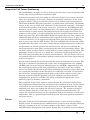
Inversion
The primary intent of offering geophysical inversion in 3D GeoModeller is to let you
test your 3D geological model against independently gathered geophysical datasets.
Provided your geological model is reasonably close to the “truth”, you can benefit from
inversion showing you aspects of your model that diverge from these datasets. Hidden
or inferred 3D structures and geometries are revealed to you and you are then able to
make adjustments to your geological model.
One of the main dangers you will face is using this tool before you have truly created
a geological reference model that is close to reality. The easiest way to check this
condition is via forward modeling. Create a grid of the forward model of your model
for say a gravitational response, and confirm that most of the main features you see
in the actual observed data are also to be seen in your forward model.
Property Optimization
With 3D GeoModeller v2012, we are also releasing technology to concentrate on
property optimization prior to any attempts at inversion. This is an important and
often neglected part of your task. The basic technology involves a least squares
deterministic search through your proposed properties for each lithology, given an
observed geophysics grid and a starting geology model.
The recommended proceedure is to then look for a set of properties that best fit over
all your project, the geology and the observed data. This usually means that you can
see if any reasonable property distributions can be found with the geometry you
propose, to explain the geophysical response. If nothing can be found that meets the
physical admissibility test, you model is not good enough to even attempt inversion.
You should be able to deduce the major weaknesses and make some re-adjustments.
This step is critical as often your rock property knowledge, especially of bulk
properties at depth, is poor.
If you cannot meet this precondition, you are going to basically waste your time
running 3D GeoModeller inversion. You are advised to continue working on your 3D
Geology model:
Contents Help | Top
© 2013 BRGM & Desmond Fitzgerald & Associates Pty Ltd
| Back |
GeoModeller User Manual
Contents | Help | Top
5
| Back |
•
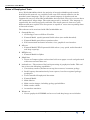
Using sections and profiles to examine the profiles of the forward model response
vs observed.
•
Using Euler depth methods to confirm your depth to magnetic basement
assumptions
•
Using multi scale edge detection, or analytical signal enhancement to get the
main faults, volcanics and basin units blocked out and constrained better.
This extra work will allow you to create a more complete model that meets the close
starting model precondition.
Scale/Resolution
A requirement to easily switch resolution of your geology model is now met in this
release when considering the geophysical response. As 3DGeomodeller builds its
geology model using an implicit function, the actual precision and resolution of the
geology model is very flexible, but as we look to a geophysical response, a hard
“Nyquist” frequency is introduced via the minimum cell size. On typical desktop
computers, a total of around 7 to 10 million cells is an upper limit. For regional
studies, with high resolution geophysical surface datasets, this can force a decimation
of your study, just so the simulation will run. This is valid for early calibration and
validating the main regional features in your model. However, there somes a time
when you may then wish to verify the high resolution response of your geology model
against the geophysics. This might take the form of say 200 million cells, and the
need to run on a cluster or in the “cloud”, using parallel computing respources to
achieve a result in a reasonable timeframe.
With this releae of 3DGeomodeller, we include the ability to directly load geophysical
survey data that is stored in lines or profiles. The tool now automatically creates
sections under each profile, making it easy for you to then do detail 2D section
interpretations and reconciliations. Examples of such datasets are aeromagnetics,
2D seismics and Full Tensor Gravity gradiometry.
Mesh Grids
In 3D GeoModeller v2012, we now support a full range of regular, semi-regular and
random point and surface datasets. This has meant that the 3D GeoModeller
Explorer now has options to fully visualize any of the grids/surfaces in 2D or 3D used
for modelling, simulation and inversion. Histograms, Data Clipping, Data Colour
Lookups, Statistical reports and Iso-Surface queries are now easy and part of the
normal workings of 3D GeoModeller. As we have a comprehensive way for you to
manage your exploration of the link between geology and geophysics datasets, there
are options to ensure your “Data Tree” explorer and your reults viewer are
automatically seeing all the transient workings. If this does not seem to be
happening, we provide a fall back for you to search and add any of these outputs to
your Tree. You can also manage the complexities by deleting unwanted simulations
as you desire.
The aim has been to also provide you with ways to visualize using the latest GPU
enhanced graphics very large Mesh/Grid datasets in the context of your implicit
geology model and to export any of the standard outcomes to a format suitable for
your needs.
External Geology Models
There are new relaxed rules for supplying a geology model in order to make use of the
Contents Help | Top
© 2013 BRGM & Desmond Fitzgerald & Associates Pty Ltd
| Back |
GeoModeller User Manual
Contents | Help | Top
6
| Back |
tools and techniques described in this reference manual. Basically, any standard
industry lithology voxet can be used. Mostly there is a need for a regular 3D grid, but
this is not an architectural requirement, as Geomodeller is moving to using
tetrahedral mesh representations of the geology as one of its outputs.
The link between the lithology key and a formation name has to be established. The
convention is to assume that the lithology is stored as an integer number and each
number corresponds to a formation. The property of the lithology voxet (Right mouse
button, bottom of list) should show this field having the “alias” set to Lithology.
This can also be done using the New Case from Voxet task described later, or simply
directly in the main 3D Geomodeller tool. Once these conditions are met, you would
Contents Help | Top
© 2013 BRGM & Desmond Fitzgerald & Associates Pty Ltd
| Back |
GeoModeller User Manual
Contents | Help | Top
7
| Back |
lauch the tool you want to use eg Forward Model Heat, and then set lithology
properties. The simulation will then be possible and the results can also be shown and
queried in the main tool.
Taking care
There is a great deal of excitement created when you have realized a geologically
sound and coherent model consistent with the sparse geological observations you
might have. However, for the unwary geologist, the further step of also making a
close match to the observed potential field data can sometimes seem bewildering and
unnecessary. It is recommened that before commencing a full scale inversion, you are
fully conversant with the simple slab inversion tutorial and all its variations. See
Appendix 4 Simple Slab Example for some of this work. Tutorial E is the dedicated
resouce to cover the material carefully.
Geologists also like to test their 3D models by systematically withdrawing each
original observation of the geology. You then recompute all of your model and save off
the surfaces and volumes for comparison with what you get from other cases. The
idea here is to test how adequately sampled your model is and also how sensitive it is
to any one observation. This process may be described by some as “Geological
Inversion”.
The great strength of the underlying 3D GeoModeller compute engine is its ability to
estimate a third dimesion in geology from the surface structural observations. We
complement this by using the independent potential field geophysics to constrain the
largest part of the uncertainty in your model.
Quantifying Uncertainty
The uncertainty you have in defining 3D geological bodies can be quantified and
characterized in many ways and by using a variety of approaches. With this release,
there exists tools for “parameter sweep”, property optimization using least squares
best fitting, tagging every observation with an error estimate and rock properties all
having a probability distribution function.
The best way to get a handle on individual geological bodies is via their volume. This
is an easier and more tractable attribute to track than the surfaces of the units.
The two preferred ways of measuring the evolution of geology bodies are:
•
Commonality, how similar is my current volume to the one I started with?
•
Shape ratio, how similar is the surface area/volume now to what I started with?
You are able to use one or both of these measures to constrain the uncertainty you
might have about parts of your model to a defined behaviour.
Of equal importance to your geological model are the property laws you must propose
for each of your units. 3D GeoModeller allows you to propose combinations of
statistical laws for each unit in your model. For instance, a Gaussian bi-modal
density distribution for one of your rock units can be proposed to cover the case where
you know you have a certain percentage of higher density material in a particular
unit. The process of inversion may then show you local concentrations of this higher
density material within that unit, enabling you to explicitly model that sub unit if you
need too.
Geoscientists are plagued by a legacy of poorly sampled and understood lithological
properties and inversion is one place where we stand exposed by this. Proposing
Contents Help | Top
© 2013 BRGM & Desmond Fitzgerald & Associates Pty Ltd
| Back |
GeoModeller User Manual
Contents | Help | Top
8
| Back |
geological unit bulk properties that are too free or have a high variability does not
allow the inversion process a proper chance to discriminate.
3D GeoModeller uses the principles of statistical sampling to drive the inversion
processes. You can think of this as a Monte Carlo simulation, Metropolis (1949). The
algorithm used has evolved quite a bit from this and concepts of topology, retaining
coherent volumes and shapes, chaos theory, all have a place. Perhaps the most
influential prior work is the paper by Mosegaard, K. and Tarantola, A., 1995.
As in keeping with the original 3D geological modeling philosophy, any observed fact
can and should be held as the “truth” during the inversion processes. Examples of this
could include an observed horizon picked from a seismic section, or the location of a
certain occurrence of a geological unit at depth, as seen in a borehole.
Currently, inversion in 3D GeoModeller takes a snap shot of the starting 3D
geological model into a voxet realization. All subsequent work is then done on the
voxet model without any back reference to the original facts embodied in the 3D
Geological model. As a consequence of this, faults are not formally honored during
inversion.
Technology Advances
The size of a simulation that can be run has also gone up a lot, as the software moves
to the new clusters and cloud computing environments, as well as being fully 64 bit
address space enabled. If you have access to 96 Gigabytes of main memory, the tools
will use this to give you accelerated capacity to do large or detailed studies.
Also, the use of Google protobuf technology to handle all the process specification and
messaging is added. This is a complete rewrite of the “batch” syntax. The protobuf
technology includes a proper parser, which explicitly informs you of any syntax errors
in a manner to help you easily make required corrections.
The lexicon of the extended geophysics process language is published with 3D
GeoModeller. It can be found in the tutorial or API directory. The actual lexicon is
“invtaskmodel.proto”. This builds on common components from the main 3D
GeoModeller geology area, as well as parts of INTREPID. So you may need to check
other “proto” files to track down allowable option settings and to see what are the
defaults and perhaps even new features since this manual was first published. A
summary of all the functions/processes available is given in appendix A.
The manual is revised to reflect this new engine room architecture. On top of all this,
several new graphical user interface improvements are made.
Each variation of Forward modelling, can be easily activated through wizard style
interfaces. Also, the full features of stochastic inversion are present in the new GUI
for that feature.
As we have also revised the 3D graphics and introduced generalised support for
handling any MeshGrid, intergrated with the Geology model, very detailed studies
are handled easily and the interaction between geology and geophysics data is much
enhanced.
Advanced API access
During 2010/2011, a couple of PhDs have been published (Monash & Curtin
Universities) that concentrate on quantifying geological uncertainty, rather than the
whole geology/geophysics uncertainty mix. The students have made use of the 3D
Contents Help | Top
© 2013 BRGM & Desmond Fitzgerald & Associates Pty Ltd
| Back |
GeoModeller User Manual
Contents | Help | Top
9
| Back |
GeoModeller published C API to directly construct geology models
programmatically, then compute the surfaces and quantify the spatial uncertainty in
3D. In one case, this was done using a Python wrapper to call the C engine room
capabilities. No C callable API exists for the main Inversion dll’s, though with the
new unified protobuf interface, the dll’s that all the functions use is accessible by
external programs, provided they construct their own messages and pass these to the
library functions. Google publish all the technology to generate C++, Java and Python
bindings to do this job. See
http://code.google.com/apis/protocolbuffers/docs/tutorials.html
Contents Help | Top
© 2013 BRGM & Desmond Fitzgerald & Associates Pty Ltd
| Back |
GeoModeller User Manual
Contents | Help | Top
10
| Back |
Status of Geophysical Tools
As at 3D GeoModeller v2012, the majority of inversion thinking and controls
detailed in this manual, are available in the new GUI wizards and also via the
protobuf control language. The V1.3 job control language is obsolete and not
supported in any way from 3D GeoModeller 2012 onwards. The tool to execute these
old commands no longer ships. The replacement tool is “invbatch”. The language is
superficially the same but greatly extended. The detail syntax is, however, quite
different and more explicit. The new parser is capable of exact error reporting down
to line and column.
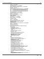
The software tools associated with 3D GeoModeller are:
1
2
Geomodeller.exe
1
3D Geology Create or Edit or Visualize
2
Forward Model spatial potential fields solver (now multi-threaded).
3
Forward Model spatial heat equation solver.
4
Full constrained stochastic inversion, via a graphical user interface.
vfilt.exe
1
3
MTDyke.exe
1
4
6
Create or Compose plans and sections laid out on paper to scale and geolocated
with extra external data sets
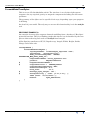
invbatch.exe - The main tool for batch processing of geophysical tasks. This tool
has at least the following capabilities 1
Uncertainty studies (Parameter sweep) for resources, basement geology.
2
Rock Property determination by least squares, best fit to regional geology/
geophysics.
3
Case Controlled Geophysical Inversion.
4
Forward Model.
5
Make Movies.
6
Make section images, including geology probabilities.
7
Make surface shells.
8
Accumulate statistics.
Worme.exe
1
Contents Help | Top
Forward Model for Dykes
jMapPrint
1
5
Forward Model FFT 3D potential fields solver ( very quick, multi-threaded
and large capacity).
Create geophysical WORMS and access a back-drop image to track faults
© 2013 BRGM & Desmond Fitzgerald & Associates Pty Ltd
| Back |
GeoModeller User Manual
Contents | Help | Top
11
| Back |
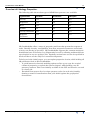
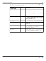
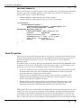
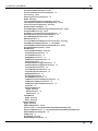
Overview of Lithology Properties.
The following table shows what types of 2D/3D data processes are available.
Type/Format
3D Grid
2D Section
3D Dykes
Gravity
yes
yes
yes
Magnetics
yes
yes
yes
Heat
yes
no
no
Seismic
no
yes
no
Gravity Gradients
yes
no
yes
Magnetic
Gradients
yes
no
yes
3D GeoModeller offers a range of properties and laws that govern the response of
rocks. Broadly, density, susceptibility, heat flow, magnetic remanence and seismic
velocity can already be specified. 3D GeoModeller supports the common statistical
distribution laws of Gaussian, Log, Exponential as well as allowing multimodal laws
up to depth 3 in any one geologic unit. Spatially variant laws can also be specified in
batch and these are the subject of current developments.
To help you in the initial stages, you can explore properties of units, while holding all
3D geometries fixed in 3D GeoModeller:
Contents Help | Top
•
A quick interactive forward modeling option to allow you to vary the vertical
column of properties to explain the observed signal, while holding your 3D
geometry constant. This is not initially available in the GUI and must be accessed
as a batch job.
•
Bounded least squares fit of a unique property value for each unit, found by
forming a matrix of contributions from your model against the geophysical
observations.
© 2013 BRGM & Desmond Fitzgerald & Associates Pty Ltd
| Back |
GeoModeller User Manual
Contents | Help | Top
12
| Back |
Stages where Inversion is used
There are several times in the process of building a 3D geological model where you
might turn to the geophysical data and ask for some guidance from it.
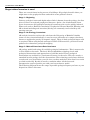
Stage 1—Beginning
Primary geological units and depths where little is known about the geology, the first
place to turn is to regional geophysical datasets. Quite a lot of information about
types of structures and geological setting of basement rocks can be quickly inferred.
Some tools such as Euler Deconvolution, Geophysical Worms, Matched Filtering and
2D sectional modeling and inversion (Naudy) are commonly used to build up the
starting concepts.
Stage 2—No Geology Constraints
3D analytic inversion, such as the code from the University of British Columbia
(www.eos.ubc.ca/research/ubcgif), is used to create 3D bodies of a compact but fuzzy
nature to explain the gravity or magnetic signal. There is little geological input used
or required. When using default settings for UBC–GIF inversions, you derive broad
guidance for subsurface geological mapping.
Stage 3—Make all Geoscience Data Consistent
3D geology model built using all available geological information. This is meant to be
a close model to the truth. The basic 3D GeoModeller technology deals with
geological observations and approaches to build the model. These geological
observations are realized in a consistent 3D sense via the rules. The rules resolve a
smoothed best fit geology of all the observations. The technology used always delivers
a result and, as a geoscientist, your job is to vet these models to drive them to a result
you find convincing. By this is meant a condition where all the facts and
interpretative aspects provide you with your best reference model.
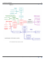
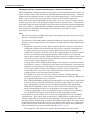
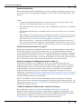
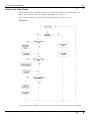
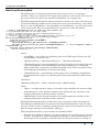
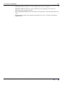
The following diagram shows the range of possible geological inputs you have at your
disposal to achieve this state.
Contents Help | Top
© 2013 BRGM & Desmond Fitzgerald & Associates Pty Ltd
| Back |
GeoModeller User Manual
Contents | Help | Top
13
| Back |
Figure 1:
3D GeoModeller Information model
Contents Help | Top
© 2013 BRGM & Desmond Fitzgerald & Associates Pty Ltd
| Back |
GeoModeller User Manual
Contents | Help | Top
14
| Back |
Taking this 3D geology model as a starting position, you now have the option to test
your model against independently observed geophysical datasets. These are typically
gravity and aeromagnetics.
A lithological constrained inversion needs to honour all ‘facts’ and then explore those
aspects of the model that are uncertain to see if a better fit to the geophysics can be
found. It is this case that 3D GeoModeller concentrates on.
In the inversion context, the geological facts are defined to be not only the original
observed contacts, but also some aspects of the 3D volumes that are created.
Currently, faults, dykes and structural dip and strikes are not honoured in the
directly inversion process. Seperate dyke modelling and inversion is available.
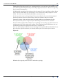
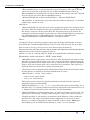
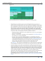
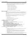
Several viable geophysical techniques are routinely used to help you gain answers to
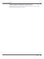
solving aspects of your undercover geology. The following diagam illustrates the use
of differing geophysical approaches that are in common use.
You can see we propose that the new technology developed in 3D GeoModeller fits at
the end of the spectrum where you already know quite a bit about your context.
Figure 2:
Relationship of geophysical inversion methods to geology
Contents Help | Top
© 2013 BRGM & Desmond Fitzgerald & Associates Pty Ltd
| Back |
GeoModeller User Manual
Contents | Help | Top
15
| Back |
Detail Outline of the Inversion Algorithm in 3D GeoModeller
The inversion algorithm can be defined using 14 steps:
1
Build the a priori geological model
2
Define the a priori physical property laws
3
Specify any a priori geological constraint properties for each unit, such as those
that are required to maintain the volume and shapes of units
4
Discretise the model to a voxel-based lithologic model
5
Specify a priori ‘fixed’ voxels, the lithology of which may not be altered eg the
mapped surface observations
6
Make a list of the geological boundary or frontier cells
7
Compute a unit-response kernel for the gravity or magnetic field or their tensor
components for each voxel at each observation location
8
Property optimization step to hone in on bulk lithology properties that join the
geology to the observed geophysics
9
Initialise the distribution of density, magnetisation, remanence and geological
constraints on the basis of voxel lithology
10 Compute the geophysical effects of the model
11 Select a voxel at random and postulate a change to the model
12 Assess the geological acceptability of the changed model
13 If geologically accepted, compute the geophysics responses of the changed model
14 Using the geophysics misfits, compute the likelihoods of the changed model
During the initial part of the inversion, the data misfit for each field of the current
model follows a generally decreasing trend. As the data misfit reaches values more in
keeping with the specified data uncertainty values, the rate of change in misfit
decreases and finally stabilizes after initial “burn-in”, and we begin to store the
models. These stored models are an exploration of the probability space of acceptable
models.
At Step 12, the changed geological model may be rejected on the basis of any one of
the geological tests, in which case the proposed change is discarded and the inversion
commences a new iteration at Step 11.
At Steps 13 and 14, each of the requested geophysics fields are computed in turn, and
their likelihood evaluated. If the changed model is rejected on the basis of a computed
likelihood, the proposed change is discarded and the inversion commences a new
iteration at Step 11. Steps 13 and 14 are repeated sequentially for each of the
requested geophysics fields (and any requested tensor components). If the changed
model is accepted on the basis of the computed likelihood for all requested geophysics
fields and tensor components, the proposed change is retained, and this new model is
stored. The inversion returns to Step 11 and continues to iterate around this loop. An
ensemble of models that satisfy geological constraints, and can satisfactorily explain
the geophysical signature might be explored by continuing for a further million
iterations.
Contents Help | Top
© 2013 BRGM & Desmond Fitzgerald & Associates Pty Ltd
| Back |
GeoModeller User Manual
Contents | Help | Top
16
| Back |
In a variation of the inversion sequence, we can also choose to use some iterations at
Step 11 to homogenise the current model. This uses morphology-based operations
applied to geological boundaries to add or remove voxels from the boundaries of
features in order to smooth them, to join separated portions of features or separate
touching features, and to remove isolated voxels (noise) from the model.
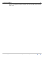
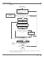
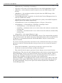
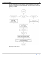
The following flow diagram is the simplified strategy used to calculate the
“lithologically” constrained inversion process. The Monte Carlo philosophy dictates
that sometimes when a modification fails its acceptance tests, it is still randomly
accepted.
Providing the starting geology model can produce a “close” geophysical response to
what was observed, there is a well behaved convergence of the model response to the
observed signal.
Figure 3:
Exploration Run
Contents Help | Top
© 2013 BRGM & Desmond Fitzgerald & Associates Pty Ltd
| Back |
GeoModeller User Manual
Contents | Help | Top
17
| Back |
Statistical presentation of inversion/simulation outcomes
Using this procedure, it is possible to generate a large number of linked models that
reproduce the gravity and magnetic observations to an acceptable degree. These can
then be analysed and combined statistically. For an inversion example, the ‘most
probable lithology above a specified threshold’ can be computed from the many stored
models, and presented as one “statistical” model. Similarly, for a heat study, a
parametric sweep through permutations of properties and boundary conditions, also
results in many linked models that reproduce the downhole temperature gradients,
surface temperatures, but also show the variability of heat flow and temperatures at
greater depths.
Advantages of joint geophysical inversion - Tensors and causative bodies
Each independently observed geophysical dataset can add something of value to
helping to validate your 3D geological model. The laws of physics are at work with
these natural manifestations. Gravitational effects from a density contrast between
geological units ( a simple contact) falls off by a square root of distance rule. Induced
magnetic effects at a susceptibility contrast junction or edge in your model falls off as
the cube root of distance. When one has access to higher derivatives of a potential
field, say full tensor gravity gradiometry data would behave a lot like induced
magnetics in terms of influence on the inversion outcomes. On the other hand full
magetic tensor data will favour shallower features in your 3D model. The big benefit
of tensor data, or even partial gradient data, is that it constitutes a direct
measurement of the curvature of the potential field. In the case of having tensor data,
we recommend you work on your geology model so that it includes honouring the
shape information that the tensor data contains.
It is common, outside of the Intrepid world, to use a “point” source as a way to model
your geology response when tensor data is at hand. The state of the art would now
include a simple way to deduce shape information in your tensor data. This requires
work on profiles of observed tensor gradients. The new capability in 3D Geomodeller
v2012 includes an “Import Dyke” option, that takes, as input, “worms” found
automatically from a set of located tensor profiles. The Intrepid tool to use is
“Naudyd”. In this way, the shape information is directly being transfered into your
geology model prior to any large scale 3D interpretation/inversion study. 5
independent tensor observations contain a lot more details about the causative signal
than just one scalar observation.
How Geophysical Signals can help your geology model
The preferred starting position when considering magnetics is to assume you can
explain all of the observed magnetic anomalies in your observed datasets with the
current Earth’s magnetic field. Often, there is no need to consider any other
explanation for the observed magnetic field.
With all of the above in mind, it is expected you will find the following:
•
•
Contents Help | Top
Gravity Only inversion:
•
Is poor for depth estimates
•
Is good for the volume or mass of geological anomaly
Induced Magnetics inversion:
•
Depth to top of body is good
•
Orientation of body is also good
© 2013 BRGM & Desmond Fitzgerald & Associates Pty Ltd
| Back |
GeoModeller User Manual
Contents | Help | Top
•
•
18
| Back |
Poor estimate of body volume
Joint Magnetic & Gravity:
•
Get both depth and volume
•
Remanence:
•
If you have existing or prior knowledge that magnetic remanence is a factor;
you will want to be able to take this into account in your model.
As above, you start out assuming that all magnetic responses can be explained
just assuming an induced magnetic field. For the next step, the primary
assumption you are required to make is the direction of the remanence vector.
This should be backed up by some field observations if at all possible. Often,
what you are reduced to doing is making a guess of the most likely average
direction. This takes the form of three direction cosines, one parallel to your
dip vector and the other two at right angles to each other and this primary
direction.
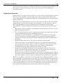
Visual Tour of Geophysical Parts of 3D GeoModeller
Setting Lithological Properties
One logical starting point is to take the geology units and give enough properties to
start to have a geophysical response. If all the units have the same property, there
will be no geophysical anomalies. The default values we give to each of the possible
properties for a unit is the same. One convention used in 3DGeomodeller is the
requirement for at least one Standard Deviation to be set to a non-zero value, as an
indication that some thought has gone into the process. See the following figures.
Figure
4
Contents Help | Top
© 2013 BRGM & Desmond Fitzgerald & Associates Pty Ltd
| Back |
GeoModeller User Manual
Contents | Help | Top
19
| Back |
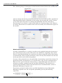
Rock Property Law Popup in 3D GeoModeller
Note in this case there are two modes for this proposal density distribution low, 20%
of 3.4 g/cc and 80% of 2.67 g/cc. The syntax shown in the Description panel has
“Normal(3.4,0.2,20) + Normal(2.67,0.0, 80)” - the first parameter is the mean density,
the second the stndard deviation and the third is the percentage of the population
following this law.
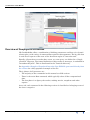
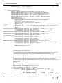
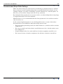
Figure 5: This shows a completed table of rock property values from a project
Contents Help | Top
© 2013 BRGM & Desmond Fitzgerald & Associates Pty Ltd
| Back |
GeoModeller User Manual
Contents | Help | Top
20
| Back |
being reported upon as one of a study’s deliverables.
An example table of Rock Properties for a study
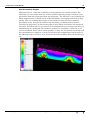
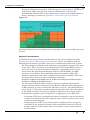
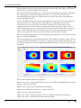
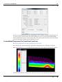
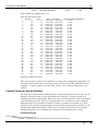
Figure 6:
Example of a section 2D forward model in a working project, showing the geology and
gravity response.
Contents Help | Top
© 2013 BRGM & Desmond Fitzgerald & Associates Pty Ltd
| Back |
GeoModeller User Manual
Contents | Help | Top
21
| Back |
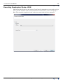
Forward Modelling Wizard
Of course, you must have a geology model before you can proceed to use this option,
so, it is expected that you have reviewed and created at least one model ( see the
Tutorials A-H). You can then choose to do 3D forward geophysics modelling. The first
page of the wizard is shown below. It is gravity and magnetics specific. The
convention used to measure and store the vector and tensor gradient field
components is also reported. Intrepid has a formal way to capture and record this in
all tools. You access this via Geophysics>3D>ForwardModel.
Contents Help | Top
© 2013 BRGM & Desmond Fitzgerald & Associates Pty Ltd
| Back |
GeoModeller User Manual
Contents | Help | Top
22
| Back |
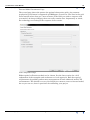
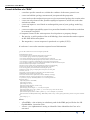
Forward Model Parameters Page
The second page shows the promts for optional observation grids. Any common
geophysical grid format is supported eg ERMapper, Geosoft etc. The data in the grid
must contain values that are a true measure of the field you wish to compare with
your model. An image (tiff/jpeg) does not really contain data. Importantly at v2012,
the technology now manages the response above terrain.
Voxet Properties Page
Either spatial or Fourier method can be chosen. See the later section for a full
explanation of the strengths and weaknesses of each approach. Each has special
requirements for padding and memory management on both 32/64 and multi-CPU
environments. The default is to use your full project extent to create a forward model,
but as you can see, there is provision for subsetting your project.
Contents Help | Top
© 2013 BRGM & Desmond Fitzgerald & Associates Pty Ltd
| Back |
GeoModeller User Manual
Contents | Help | Top
23
| Back |
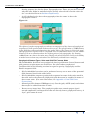
Variable Z
By selecting the Variable Z option the user can create a semi-regular voxet instead of
a regular voxet (See image below). This allows the user to define a voxet geometry
where the cell size can vary with depth. The cell size near the surface can be small
and then after a nominated depth start to become progressively larger. This gives a
better resultant forward model more efficiently than by using the smaller cellsize
throughout the voxet.
Contents Help | Top
© 2013 BRGM & Desmond Fitzgerald & Associates Pty Ltd
| Back |
GeoModeller User Manual
Contents | Help | Top
Contents Help | Top
24
| Back |
© 2013 BRGM & Desmond Fitzgerald & Associates Pty Ltd
| Back |
GeoModeller User Manual
Contents | Help | Top
25
| Back |
Properties Page
This page in the wizard adapts to the quantity for which you wish to model the
response.
You should review, or set your required estimates of density etc. distributions for
each unit, as required.
Runtime Settings Page
Contents Help | Top
© 2013 BRGM & Desmond Fitzgerald & Associates Pty Ltd
| Back |
GeoModeller User Manual
Contents | Help | Top
26
| Back |
Results Explorer
This “results explorer” tool is designed to help you explore the misfit of your forward
model data against any available observed grids from the same geophysical
phenomenon. As there are usually long wavelength trends in the observed data that
can not be explained by your model, we also give simple trial and error access to trend
fitting and removal, to help you to see if your forward model is adequate in explaining
those frequencies and wavelengths that the model can represent. This feedback is
done by also storing the “spatial response kernels” and then in real time, adjusting
your model.
You are advised to review Tutorial E, as this is specifically written to cover much of
the basics for the new user wanting to learn how to use the geophysics capabilities.
Contents Help | Top
© 2013 BRGM & Desmond Fitzgerald & Associates Pty Ltd
| Back |
GeoModeller User Manual
Contents | Help | Top
27
| Back |
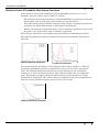
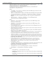
Figure 7:
Example: Improvement of misfit during inversion. The blue cases are for prior geology
only and make no reference to an independent geophysical dataset. Hence, they reflect
the geological uncertainty of the model. The other cases show an initial misfit, that
reduces to a “converged solution”. It is from this point on that 3D GeoModeller begins
the job of gathering statistical information about your model.
Figure 8:
Initiating a limited inversion run via the older graphical interface options
Inversion Wizard
All the geophysical process wizards have a similar look and feel to each other. The
stochastic inversion wizard starts the same as the forward modelling and then the
extra options and settings are presented, following the case/run/execute flow.
Each page in the wizard corresponds to the important parameters to be set
Page 1 - choose Case/Run
Contents Help | Top
© 2013 BRGM & Desmond Fitzgerald & Associates Pty Ltd
| Back |
GeoModeller User Manual
Contents | Help | Top
28
| Back |
Page 2 - choose observed grids, and properties and response to calculate eg Gravity
Page 3 - set the main case control parameters
Page 4 - set the main run control parameters
Page 5 - set the overall controls, number of iterations,
Page 6 - final decisons about the Batch/Interactive/Cloud and submit.
If running interactively, a progress misfit is shown. When finished, a prompt for
generating a Statisical analysis is given.
A simple check that the requested property distributions have been honoured while
performing the inversion can be made by examining the individual finishing position
property histogram for each lithology unit against what was requested at the start.
Contents Help | Top
© 2013 BRGM & Desmond Fitzgerald & Associates Pty Ltd
| Back |
GeoModeller User Manual
Contents | Help | Top
29
| Back |
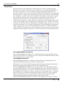
Heat Uncertainity Studies
With this release, comes the capability to do parameter uncertainty studies. The
following is a screen shot after one of these studies relating geology, heat flow, heat
production from buried granites that are radiogenic. The aim here is to constrain the
likely temperatures at depth, given all the knowledge of rock properties and geology
setting. The way of doing these types of uncertainty studies has been termed a
parameter sweep. You specify which of the boundary conditions and rock units
(variables in play) have an uncertainty that is most likely to influence the predicted
outcomes. You then select if you want 2 or 3 variations for each of these variables eg
minimum, mean, maximum. For instance, if there are 5 variables, either 32 or 217
cases are defined. These can be run in parallel, as they are all unrelated, and when all
the simulations are complete, a staticical analysis and compilations can be made in
the 3D model space to form a view about the overall varaibility that you are likely to
see.
Contents Help | Top
© 2013 BRGM & Desmond Fitzgerald & Associates Pty Ltd
| Back |
GeoModeller User Manual
Contents | Help | Top
30
| Back |
Definitions and Management of Workflow Scenarios
Two terms that are used throughout this document are Case and Run:
•
Case - combines the a priori information with the observed data, and is thus a
geological or geophysical hypothesis or scenario which we propose to test. It is a
geological model, together with knowledge of the physical properties of the
geology formations, and it is also a set of geophysical (gravity, magnetics)
datasets, and such auxiliary data as the definition of the Earth’s magnetic field
parameters for the particular project area.
•
Run —an actual execution of a 3D GeoModeller process, based on a particular
Case. For a given geological or geophysical scenario, there are many ways that a
Run might be executed—by setting controls that constrain the way in which an
inversion or simulation can proceed. Thus a Run contains the specifications of all
Run control parameters, and also the full set of results from the Run. Results are
primarily the complete set of proposed changes to the geology model that were
accepted during the particular Run. There may be one or more Runs associated
with an inversion Case.
A Case, and one or more associated Runs, are represented symbolically in Figure 9:
Other terms used extensively in this document are:
Contents Help | Top
•
Project is a 3D GeoModeller Project. A Case contains a copy of a 3D
GeoModeller Project. The 3D GeoModeller geological model must have been
computed (the inversion derives the geology voxel model from the computed model
in the 3D GeoModeller Project).
•
MeshGrid - is any 2D or 3D regular, irregular grid or surface. With the new
version of Geomodeller, the underlying systems libraries from Intrepid now
include a fully systematic way to store these MeshGrids in a binary form, together
with all the extended metadata. Any data type, eg Integer, Float, Date, Boolean,
Vector. Partial support for Tensor grids is also present. Unlike the “line” or profile
ways to gather and store most original observations of geophysics, this variant
concentrates on random point data, and grids. However, full geophysical
databases can now be introduced into Geomodeller as these MeshGrids of random
point observations. Kriging can then be used to produce grids.
•
Voxet is a special case of MeshGrid and in particular, the 3D lithology model can
be stored as an “integer” geology voxet. There may be several different Voxets in a
Case. The Case Voxet is the voxel lithology model derived from the 3D
GeoModeller Project when a Case is created. A Run has an Initial Voxet
(typically derived from the Case Voxet), and a Final Voxet, being the final geology
model of some inversion Run (which might then be used as the start of another
Run). The full 3D voxel geology model at any given iteration in a Run can also be
generated again, as a Voxet. The Reference Voxet—used as the reference geology
model against which the current model might be tested during a Run—is also a
Voxet (It is often the same as the Initial Voxet, but it need not be). Note that
‘voxet’ is also a generic term, referring to any file of voxels (3D) in the GoCAD
voxet format. In these notes, Voxet (with uppercase ‘V’) refers specifically to a 3D
geology model.
•
Kernel is the geophysical unit response function used to record the geophysical
response—at the designated measurement elevation—for every possible voxel in
the 3D geology model Voxet (and its surrounding buffer zone), for each of the
required geophysical data types (for example, magnetism, gravimetry, vertical
gradient of gravity (Gdd)), and for ‘unit’ physical property contrast (for example:
for unit density). The Kernel is computed once, and stored (for reuse in later
© 2013 BRGM & Desmond Fitzgerald & Associates Pty Ltd
| Back |
GeoModeller User Manual
Contents | Help | Top
31
| Back |
Runs).
Figure 9:
Symbolic representation of an inversion Case, and one or more associated inversion
Runs.
Figure 10:
3D GeoModeller inversion flowchart, showing the main persistent data objects, and the
Contents Help | Top
© 2013 BRGM & Desmond Fitzgerald & Associates Pty Ltd
| Back |
GeoModeller User Manual
Contents | Help | Top
32
| Back |
executable commands used to generate inversion results and reports
Contents Help | Top
© 2013 BRGM & Desmond Fitzgerald & Associates Pty Ltd
| Back |
GeoModeller User Manual
Contents | Help | Top
33
| Back |
Support for Full Tensor Gradiometry
3D GeoModeller can make use of any of the measured scalar, vector components and
second order tensor gradients of a potential field.
A predicted response from your model of a full tensor signal at an average elevation
above the topography can be made. Support for magnetic remanence in any of the
geological units is also given and this can be made to influence the forward model.
The Forward Model FFT option generates a genuine tensor grid rapidly. The Results
viewer, in the case of tensor data, shows one of the magnitude measures - Cube Root
of the Second Invariant of the tensor curvatures. You must use the ERMapper grid
format to get this result ( nb Oasis Montaj does not support multi-band grids and so
cannot manage a tensor signal). The Intrepid Visual tool (Geophysics>Visual) also
supports tensors grids, so a fully exploration of all the possible enhancements can be
made using that tool. 3D GeoModeller MeshGrid support does not fully embrace the
underlying Intrepid object oriented data object approach at this release. It goes as far
as vectors. However, we do expose the Intrepid tensor grids for forward modelling
from a voxet, especially the FFT method. The dyke modelling also includes the ability
to handle full tensor data, as a tensor. Improvements will be progressively made here.
As the number of observed parts of the field increases, the process of driving the
inversion towards a most likely convergent model takes correspondingly longer. The
stochastic solver tends to scale in a linear fashion as more components are added. The
philosophy for the scalar case is to spend 50% of the time on the property law and
50% of the time perturbing the geological unit boundaries. The question to ask is can
we maintain this ratio and somehow optimize honoring the full tensor signal and the
model convergence?
Recent work by Intrepid on tensors develops the notion of separation of concerns. This
has lead to a patent for preparing the survey data for interpretation via a gridding
(SLERP) and curvature integrity smoothing process ( MITRE) . Approximately half
the useful signal resides in the Gzz component for inversion, so use the complete
tensor if available. Much of the detail shape information from the geology bodies that
are causing the anomalies in the first place lies within the curvature as captured by
the full tensor. Intrepid supports tensor grids so that all the signal is in one place,
properly registered and also properly processed. With the new 64 bit memory
computers now generally available, the ability to handle this signal type is not
limited by speed or memory constraints.
The amplitude of the tensor signal is separated from the orientation of the tensor.
The amplitudes or Eigenvalues are invariant to the coordinate system. In the context
of inversion, the local rotations of the signal may be less important than the signal
amplitude as a driver for making the inversion converge. The number of terms of
concern changes from five to two and so is very significant computationally. Of
course, the occasional iteration can be scheduled to look at the rotations as well as the
amplitudes. This is a proposed optimization step for full tensor gradient inversions
for future release.
Falcon
Also part of this mix is the horizontal gradient tensor, as measured by the Fugro
Falcon system. It warrents special consideration as it too has more integrity than just
treating a component of the curvature gradient as the signal - there is extra
embedded phase information in the signal. During 2011, a workflow to process Falcon
Contents Help | Top
© 2013 BRGM & Desmond Fitzgerald & Associates Pty Ltd
| Back |
GeoModeller User Manual
Contents | Help | Top
34
| Back |
and then develop techniques to utilize the full signal during interpretation has been
developed. It is expected to deploy some of the outcomes in 3D GeoModeller
inversion in 2012.
Support for Seismics
At the lowest level, each rock unit can have a seismic velocity. 3D Geomodeller v2012
also has a new capability to import and analyse micro-seismic point clouds with a
view to interpretation of unknown fault planes and jointing that a fracturing program
might be inducing.
Currently, the recommended way to create a 3D velocity model is to use the “domain”
kriging feature. If you have 2D seismic shot point data, you can choose to work in
time or depth. Either way, the mechanism to get an optimum velocity model
constrained by a proper geostatistical analysis of your data involves the following
steps.
•
Import the seismic section data, including the shot points and velocities. Use the
3D observed points option.
•
It is recommened that you create a 3D geology model of the sedimentary geology
using the standard 3D geology modelling techniques.
•
Create one or more variograms of your velocities, constrained by each geology
unit. This is known as “domain” kriging. Your seperation distances between
samples is calculated following the trends of the geology model ( implicit model
potentials).
•
Interpolate the velocities for each unit for which have observations.
•
You can also choose to convert the velocities to an estimated density and then
calculate a gravity response. This can then be compared to any surface gravity
observations you may have. This process is very useful in independently
validating the main geology picks from the seismic sections.
•
Unconstrained kriging can also be used to interpolate in 3D your velocity or
density estimates from the 2D seismic data. This is a much more problematic
approach, as you are ignoring any breaks in the rock fabric.
•
The conversion of velocities to densities is often done by a simple equation. This is
easily done using the MeshGrid fields and the equation builder functions. Support
for a table lookup to convert and/or a spatially based equation is also supported.
Below is an example of a 2D seimic section predicted by assigning velocities to each
unit, then doing a forward model on a section. You can get radically different results
by changing the sample spacing and time sampling, so this provides a simple way to
appreciate the impotance of survey design parameters vs the seismic data predicted
vs the geology scenario. It is easy to say commission a survey that in fact does not
lend much new knowledge to the deeper strata and the rock relations.
Contents Help | Top
© 2013 BRGM & Desmond Fitzgerald & Associates Pty Ltd
| Back |
GeoModeller User Manual
Contents | Help | Top
35
| Back |
Overview of Geophysical Processes
3D GeoModeller offers a combination of defining parameters and laws via a formal
schema plus a rich variety of command line options with arguments. The key file that
is used for all aspects of the state of the Inversion engine is “inversion.xml”.
Equally, all procedures or tasks that create, set, run query, are defined in a Google
“protobuf” language. The formal definition of these tasks or messages, is embodied in
“invtaskmodel.proto”. This is distributed in the Tutorials directory.
See Appendix 3 Sample of Populated Inversion Case XML file generated directly from
the schema for a fully populated example of the file.
The 3 phases of all processes are:
•
The majority of the commands in this manual are Edit actions.
•
There is the main Run command, which typically takes all the computational
time.
•
The last phase is to Query the results, making movies, snapshots and other
reports.
As an aid, each command in the following sections is classified as belonging to one of
the above categories.
Contents Help | Top
© 2013 BRGM & Desmond Fitzgerald & Associates Pty Ltd
| Back |
GeoModeller User Manual
Contents | Help | Top
36
| Back |
Statistical Laws & Probability Distribution Functions
At the heart of much of the thinking in 3D GeoModeller Inversion, is a set of
stochastic processes that respect statistical models:
•
The main potential field interpolator in 3D GeoModeller is based upon universal
dual kriging, and as such represents a high level of geostatistics.
•
The models that govern allowable changes in the volumes of geological bodies are
constrained to follow Exponential or Log Normal distributions.
•
Finally, the lithological properties that you are required to specify for all your rock
properties, also respect laws such as Normal, Lognormal.
Each of these models has a well defined and well understood mathematical basis.
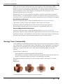
The following diagrams represent normal and log normal probability distribution
functions.
Gaussian/Normal distribution
Log Normal Distribution
For constraining the geometry of the geological bodies (their volumes), a Weibull
probability distribution function is introduced to give access to more appropriate
rules. The Weibull distribution has gained a large following in the automotive
industry as a means of predicting mean time between failures for car component
parts. The property sought is that the initial starting model should have a high
probability of being right. This follows from the proposition that the geologist knows
what he is doing and the reference model is close to the truth.
Weibull probability distribution
Contents Help | Top
© 2013 BRGM & Desmond Fitzgerald & Associates Pty Ltd
| Back |
GeoModeller User Manual
Contents | Help | Top
37
| Back |
The need for a Close Starting Model
One of the central issues needed for a successful use of the fully constrained
lithological inversion method, is to create a starting or reference model that is not
only consistent with all the geological observations, but also “close” to honoring the
observed geophysics signals for the majority of your study area.
The simple reason for this requirement follows from the use of Monte Carlo
techniques which will not converge to an appropriate solution if the initial model is
grossly incorrect. There is a very detail process of changing individual properties or
geometries. A close starting model ensures you maximize the likelihood and minimize
the time needed to explore the relevant part of probability space to firstly converge to
an acceptable misfit, and then continue through gathering good statistical results.
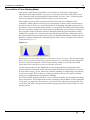
Taking the example case of having an observed gravity grid and a forward model of
the gravitational response from your model, you should immediately examine the two
grids for a spatial comparison. A histogram provides a way to examine the statistics,
as shown in Figure 11:.
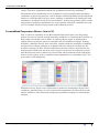
Figure 11:
Illustration of a non-viable reference model prior to any inversion. The left hand population from a forward model of the gravity response is a completely different distribution to the observed response. The average starting misfit is more than 200 mGal
(horizontal axis), and far too much to consider inversion.
In the situation shown, the likelihood of your starting position migrating to the
required observed position, while also honouring the known constraints, is very low.
It is for this reason, you are advised to continue working on improving your starting
or reference model. This is done by looking at problem areas via sections, making
changes and updating the 3D forward modelling.
To retain realistic geological bodies, you are advised to make use of volume and shape
ratio constraints. A full explanation of the workings of these follow. If this constraint
is not used, an apparent conversion to a good fit can be achieved automatically, but
you will be left with a fragmented predicted geology that bears little relation to your
staring model.
Contents Help | Top
© 2013 BRGM & Desmond Fitzgerald & Associates Pty Ltd
| Back |
GeoModeller User Manual
Contents | Help | Top
38
| Back |
Case Management
To cope with the possibility of many scenarios that you may wish to pose, 3D
GeoModeller introduces the concept of Case Management. This is common to both
GUI and batch thinking.
A 3D GeoModeller Case is a collection of the data components that are common to a
set of Runs:
•
A geology reference model
•
The associated characteristics of the geological formations
•
The one or more geophysical grids to be used (jointly)
•
The specification of the voxel divisions of the geology model.
Use the NewCase and CaseControl commands to create, and then configure a 3D
GeoModeller Case. Conceptually, one would use these commands to set up a
particular Case and then perform a series of Runs based on that Case.
In general, once you have commenced Runs on a given Case, you would not modify the
Case properties. Instead, if changes are required, you would create another Case—
with the required new Case properties—and then perform further Runs on that new
Case.
The components and properties of a Case are:
Contents Help | Top
•
A Case geology model, which is a copy of a 3D GeoModeller Project, copied to a
nominated Case subdirectory (NewCase command).
•
The specification of the ‘division’ of the geology model into a geology Voxet. The (x,
y) division of voxels is determined from the geophysical grids; the (x, y) voxel
positions and dimensions are aligned exactly with the grid cells of the geophysical
grids. The z-division of voxels is specified in the NewCase command.
•
For inversion, specification of the extent to which the geology formations of the
geology Voxet are moveable, or are held ‘fixed’ (SetFixedCells command); this
captures the project geologist’s knowledge of the reliability of the geology model,
which portions are constrained by observed geology that must be honoured, and
which parts are less reliable, and hence allow more scope for change to the model.
•
A specific representation of the surface topography, derived from the 3D
GeoModeller Project (NewCase command), and specifications regarding use of
the topography in generating the lithology Voxet, and the assignment of physical
property values to the ‘above topography’ region (CaseControl commands).
•
Properties of the geology formations (From the 3D GeoModeller Project or
updated by CaseControl commands). These are the physical property data for
each geology formation, but also include special inversion-related properties of
formations ie controls the amount of fragmentatio n that is acceptable.
ShapeRatio, (defined as the square root of surface area divided by cube root of
volume) for example, specifies the degree to which an inversion Run must
maintain the ratio of a formation’s surface area to volume.
•
The set of one or more geophysical grids to be used. All grids must have exactly
matching grid cell size and positions. Associated parameters: the height of
observation for each dataset must be specified, and (for magnetics data) the
Earth’s magnetic field intensity, inclination and declination are required for
computation of magnetic responses.
© 2013 BRGM & Desmond Fitzgerald & Associates Pty Ltd
| Back |
GeoModeller User Manual
Contents | Help | Top
39
| Back |
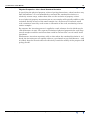
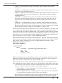
NewCase
The NewCase command sets up a new inversion Case, which will then be used as the
basis for a set of one or more Runs.
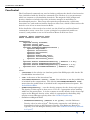
Formal Syntax for creating in batch:
invbatch -batch <taskfile.task>
where <taskfile.task> contains:
NewCase {
filename: "<Project>";
case: "<Case>";
x_cell_size:<xCellSize>;
y_cell_size:<yCellSize>;
z_cell_size:<zCellSize>;
east_minimum_voxet:0.000000;
east_maximum_voxet:1000.000000;
north_minimum_voxet:0.000000;
north_maximum_voxet:1000.000000;
elevation_minimum_voxet:<ElevationMinVoxet>;
elevation_maximum_voxet:<ElevationMaxVoxet>;
ObservedGridList {
ObservedGrid {
type: Magnetism;
mean_elevation: <MeanElevation>;
compute_surface_style: ConstantElevation;
precision: <Precision>;
Match_Trend: <MatchTrend>;
Match_Trend_Degree: <MatchTrendDegree>;
Match_Trend_Rate: <MatchTrendRate>;
grid: "<GeophysicsGrid>";
}
}
}
Where:
Contents Help | Top
•
<Project> is the relative (or absolute) path and Project name for the source 3D
GeoModeller Project, from which the Case will be derived.
•
<Case> is the Case identifier or name, and will also be the name of a subdirectory
of the <ResultsDir>, within which the Case files will be written.
•
<zCellSize> is the Z-height (in metres) of the voxels of the geology Voxet to be
derived from the 3D GeoModeller geology model.
•
<ElevationMinVoxet> is the vertical elevation of the base of the bottom voxels.
See note below regarding the use of ElevationMaxVoxet relative to
ElevationMinVoxet to define the z-range of voxels in the geology voxel file.
Default is to set this base at the bottom of the 3D GeoModeller project.
© 2013 BRGM & Desmond Fitzgerald & Associates Pty Ltd
| Back |
GeoModeller User Manual
Contents | Help | Top
40
| Back |
•
<ElevationMaxVoxet> is the (maximum) vertical elevation of the top of the top
voxels. See note below regarding the use of ElevationMaxVoxet relative to
ElevationMinVoxet to define the z-range of voxels in the geology voxel file. Default
is to specify the top of the 3D GeoModeller project.
•
<MeasuredGridsList> is MeasuredGridsList1 ... MeasuredGridsListN
•
<ResultsDir> is automated to put order into the situation. Basically, a Case/Run
subdirectory scheme is used.
And where:
•
<MeasuredGridsList> specifies each of the geophysical grids to be included in the
inversion. Each list nominates the type of geophysical dataset, specifications for
the dataset, and user choices about how the inversion process will ‘match’ the
computed and observed grids for that dataset. <MeasuredGridsList> parameters
are: <Geophysics Type> <MeanElevation> <Precision> <MatchTrend>
<MatchTrendDegree> <MatchTrendRate> <GeophysicsGrid>
Where:
<Geophysics Type> specifies geophysics data type from the following list as reproduced from the “commontaskmodel.proto” file ( see the API directory for up to date
list): Gravimery,Gxx,Gyy,Gzz,Gxy,Gxz,Gyz,Gee,Gnn,Gdd,Gen,Ged,Gnd,Gz,
Magntism,Mxx,Myy,Mzz,Mxy,Mxz,Myz,Mx,My,Mz,Mee,Mnn,Mdd,Men,Med,Mnd,Me,Mn,Md,
TMI,Temperature,GravityTensors,MagneticTensors;
where e = east, n = north, and d = down in a right hand coordinate system
(Remember: ‘north east down’ = NED—right hand).
•
<MeanElevation> is the survey observation level for this dataset (in metres). Note
that this is not ground clearance, but a true vertical elevation, using the same Zpositive-upwards vertical datum and scale as used in the source 3D GeoModeller
Project. Also, an elevation grid can be specified if it is available. This option is a
fall back when you do not have a drape elevation grid.
•
<Precision> is the estimation of the standard deviation of the measurement errors
for this dataset, assuming a Gaussian distribution of errors
•
<MatchTrend> = < false | true> where:
•
false= do not match trend;
•
true = yes, match trend.
This refers to the removal of regional gradients or trends from the observed
geophysical dataset (detrending).
Contents Help | Top
•
<MatchTrendDegree> = < 0 | 1 | 2 | 3 > specifies the degree of detrending; 0 is a
DC shift only; 1 is a planar gradient trend across the dataset. Recommend use 0 or
1. Options 2 and 3 introduce more curvature into the detrending.
•
<MatchTrendRate> is the repetition rate—in terms of numbers of iterations—for
applying the detrending. To apply detrending once only (at the start), specify ‘0’.
•
<GeophysicsGrid> is the relative (or absolute) path\filename of the geophysics
grid data file. The range of grid format files supported can increase as more
drivers are added to Intrepid and made available to this context. ERMapper ,
Oasis Montaj and an ASCII format known as “semi”, are core formats.
© 2013 BRGM & Desmond Fitzgerald & Associates Pty Ltd
| Back |
GeoModeller User Manual
Contents | Help | Top
41
| Back |
The Z elevation of voxel centroids will range from
ElevationMaxVoxet – nZ × zCellSize + zCellSize / 2 to
ElevationMaxVoxet – zCellSize / 2
where nZ = Number of horizontal sheets of voxels in the geology Voxet such that
ElevationMaxVoxet – nZ × zCellSize <= ElevationMinVoxet and
ElevationMaxVoxet – (nZ + 1) × zCellSize < ElevationMinVoxet.
Thus, the Z division of the 3D GeoModeller Project into voxels is calculated from the
specified top (ElevationMaxVoxet), then working downwards until the lower limit is
reached. That lower limit does not need to be specified ‘exactly’.
The NewCase command:
•
Creates a <Case> subdirectory in the project directory
•
Copies the 3D GeoModeller Project to that directory, with Project name <Case>
•
Copies the input (field, observed) geophysical grids to that directory
•
For an inversion run, we create the inversions.xml file; this file is used to record
all parameter settings for the Case, and for subsequent inversion Runs performed
for that Case.
•
Creates the <Case>.vo file; a GoCad voxet with the Lithology as a field. Lithology
is coded as integers; 0 = the above topography region, and 1, 2, 3 are the indices
for the geological formations (which are listed in the corresponding order in the
inversions.xml file.
The NewCase command brings together a range of geology and geophysical datasets
to create the Case. You need to ensure that the datasets are compatible with each
other and compatible with the way in which 3D GeoModeller geophysics tools
operate. The following Notes add further important details to supplement the
definitions in the above Syntax.
Dataset Requirements
Geology Project
3D GeoModeller uses a 3D GeoModeller Project as the primary source of knowledge
about the geological structural of the project area. The 3D GeoModeller Project also
serves as the source of the surface topography (See Surface Topography). Note,
however, that it is possible to perform an inversion with a Gocad geology model,
provided the extra information needed is also presented
The main requirements for the 3D GeoModeller Project are:
Contents Help | Top
•
The model must have been computed. This means that if any last minute edits are
performed in 3D GeoModeller, the model must be recomputed before using that
Project for geophysical forward or inverse modelling.
•
If the reporting of inversion results will use images of inversion—geology results
or movies of the inversion’s evolution-of-the-model on sections, then those sections
must have been previously created in the 3D GeoModeller Project. Both
traditional vertical sections and horizontal slice sections may be created and used
in the reporting of inversion results.
•
An external Gocad voxet is used to create a 3D GeoModeller project via the
“New” command. Once a project is created, sections can be added to the project, so
that you can use these to create images and movies that are geolocated.
© 2013 BRGM & Desmond Fitzgerald & Associates Pty Ltd
| Back |
GeoModeller User Manual
Contents | Help | Top
42
| Back |
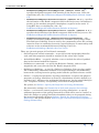
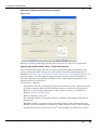
Figure 12:
Simple slab model to illustrate principles of inversion. You have even in this simple
case, a geometry and the need to specify properties.
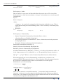
Physical Properties
•
The specification of the physical properties of each geology formation can either be
predefined in the 3D GeoModeller Project, or can be set later by using
CaseControl commands. The NewCase command records the physical property
settings (or their default values) in the inversions.xml file of the Case.
•
Likewise, the specification of the Reference Density may be predefined in the 3D
GeoModeller Project (or left at its default setting: 2.67 g/cm3). The density for
each voxel in the geology model, relative to the Reference Density, determines a
density contrast for that voxel, from which the model’s gravity response is
computed. The Reference Density should typically be that density value used for
the Bouguer data reduction of the observed gravity data if Bouguer gravity data
are supplied, or the mean density of the region if Free Air gravity data are used.
The NewCase command records the Reference Density in the inversions.xml file
of the Case.
•
Use the CaseControl commands (see CaseControl) to further modify these
physical property data for the Case.
Surface Topography
The surface topography for the project area is sourced from the 3D GeoModeller
Project. Note that 3D GeoModeller describes modelled geology interfaces that extend
throughout the volume of the 3D GeoModeller 3D Project space such that, by
default, geology boundaries can extend above the topography into the ‘air’!
Considerations with regard to surface topography are:
Contents Help | Top
•
The ‘top of the model’—set with the <zMaxVoxet> parameter—should be set such
that the topography and the Earth’s near-surface region are included in the model
See Figure 13: (b).
•
You must explicitly declare that the surface topography should be taken into
account by using the CaseControl SetUseTopo command (IncludeBorderEffect); in
effect, this command creates another ‘lithology’ for those voxels where the voxel
centroid is at an elevation above the topographic surface. In this manual we refer
to the Above Topography zone or region.
•
An inversion of an observed field on the topography surface is supported, as well
as observed data from an aeroplane.
•
The default values for the magnetic susceptibility and remanence of the Above
Topography zone are ‘0’, and cannot be altered. The default density value,
however, is the same default density as for every other geology formation—the
Reference Density value, and not the density of air! The CaseControl
SetAboveTopoDensityLaw (SetAboveTopoDensity) is used to specify the required
© 2013 BRGM & Desmond Fitzgerald & Associates Pty Ltd
| Back |
GeoModeller User Manual
Contents | Help | Top
43
| Back |
density property law for the Above Topography zone. There are practical reasons
why this zone might be modelled with a density value which is not the value for
air—see the discussion in SetAboveTopoDensity.
•
A cell is defined to be above the topography when its centre is above the
topographic surface.
Figure 13:
The effects of surface topography are always a component of the observed geophysical
responses for both ground and airborne surveys (a). The specification of <zMaxVoxet>
in the NewCase command determines the upper limit of the Voxet, for which the modelled geophysical response will be computed. The recommended choice is to set <zMaxVoxet> to be at an elevation above the highest point of the topography (b). Setting
<zMaxVoxet> at a lower elevation may simplify the model, but also removes the ability
to model sources that may exist above the arbitrarily selected lower cutoff (c).
Geophysical Dataset Types, Units and Grid File Formats Grids
3D GeoModeller Inversion uses geophysical data in grid format. Several dataset and
grid geometry requirements are noted here. See also further geophysical
considerations in the following sections in regard to gravity, topography and the
Earth’s magnetic field:
Contents Help | Top
•
3D GeoModeller Inversion can be performed on any one or more of the potential
field datasets listed in the table below.
•
3D GeoModeller computes geophysical responses in terms of the units noted in
the table and so the observed geophysical grid data must be supplied in terms of
these same units. (For unit conversions, see Appendix 1 Units and Units
Conversions).
•
Allowed grid file formats: ERMapper (ers), Geosoft (grd), ASCII (semi) and others
that maybe be added from time to time.
•
Do not use an image here. The geophysics grids must contain proper signal
strenth amplitudes and frequencies that are directly from a geophysical survey. A
“byte” grid cannot be used.
© 2013 BRGM & Desmond Fitzgerald & Associates Pty Ltd
| Back |
GeoModeller User Manual
Contents | Help | Top
44
| Back |
This table shows the geophysical data types, and units allowed in 3D GeoModeller
joint Gravity and Magnetic Inversion
Contents Help | Top
Data type
(and key word)
Units
Description
Gravimetry
mGal
Conventional gravity data as measured
using a Z-downwards frame of reference.
Since the Z-downwards direction is
determined by the gravity vector itself(!),
‘conventional’ gravity is ‘total’ gravity field
strength.
Ge,Gn,Gd
mGal
Vector components of gravity data, where
e = east, n = north, and d = down in a right
hand coordinate system.
Gee, Gen, Ged, Gnn,
Gnd, Gdd
Eotvos
The components of the gravity gradient
tensor
Magnetism
nT
Conventional total magnetic intensity
(TMI) data
Me, Mn, Md
nT
Vector components of magnetic intensity,
measured in the east, north and Zdownwards directions.
Mee, Men, Med, Mnn,
Mnd, Mdd
nT/m
The components of the magnetic gradient
tensor, where e = east, n = north, and d =
down in a right hand coordinate system.
© 2013 BRGM & Desmond Fitzgerald & Associates Pty Ltd
| Back |
GeoModeller User Manual
Contents | Help | Top
45
| Back |
Geophysical Grids—Vertical Considerations—Acquisition Elevation
3D GeoModeller computes geophysical responses—for all geophysical data types—at
either a single, fixed vertical elevation (the <MeanElevation> parameter), a constant
heigth above the ditigital terrain, or onto a provided drape surface. By elevation we
mean a ‘true’ vertical elevation, specified in terms of the Z-positive-upwards
framework of the 3D GeoModeller geology model; it is not a survey height or mean
terrain clearance. Of course, geophysical signals such as gravity, have a convention of
the field being given with Z positive down. From here we start the need to distinguish
between geometry, a right handed coordinate system in East, North Up for XYZ and
conventions the geophysics field might be measured in. (possibly the same
convention, but often not).
Thus:
•
For joint inversion of multiple data types, all geophysical grids can have varying
effective acquisition heights.
•
In contrast to 3D GeoModeller computed solution at constant elevation, typical
airborne survey observations are recorded at variable elevation! The implications
of this are:
•
Magnetics: In practical terms, many regional airborne surveys are flown at a
sufficiently uniform elevation that the data can be regarded as having been
acquired at the mean survey elevation. If the dataset must be upward
continued (see below), then the error in this approximation is further reduced.
In some circumstances this approximation would introduce unacceptable
errors; these might include significant height variation in rugged terrain, and
low level surveys, where the (varying) elevation of survey observations was
close to near-surface magnetic sources.
•
Gravity: Observation height and the shape of the terrain are important factors
in all gravity surveys, so the Free Air, Bouguer and full terrain corrections are
applied to gravity datasets. The Bouguer or terrain corrections treat the Earth
as having a uniform density (the Bouguer density), and are designed to
remove the gross error due to the contrast between earth and air, and the
complex shape of the boundary between them.
The Earth, of course, does not have uniform density, and the observed
geophysical response to a near-surface anomalous mass within the Earth may
vary significantly with survey elevation.
•
Since 3D GeoModeller geophysical computations are voxel-based, with voxels
having a discrete z-height (<zCellSize> specified in the NewCase command),
these computations do not achieve a reliable modelling of the topography.
With 3D GeoModeller v2012, we have introduced new technology to adapt
the detail modelling to allow you to minimize any stepped effects. The
‘stepped’ topography of the voxel-modelled surface can generate artefacts in
any geophysical solutions computed close to the topographic surface.
An alternative, crude solution is to exclude the topography from the modelling
computations. This can be done by setting the <zMaxVoxet> parameter at an
elevation below the lowest point of the topography. This means that the computed
solutions will be derived from a simpler, flat topped model where the upper parts
of the Earth have been sliced off, but it also assumes that there are no signatures
in the observed data that have been derived from sources above that arbitrarily
selected cutoff for the top of modelled data! See Figure 13: (c):
•
Contents Help | Top
For magnetics, this will be true where the near-surface geology is non© 2013 BRGM & Desmond Fitzgerald & Associates Pty Ltd
| Back |
GeoModeller User Manual
Contents | Help | Top
46
| Back |
magnetic, such as across a sedimentary basin.
•
For gravity, it would require that the gravity data were fully terrain-corrected,
and that the geology above the selected cutoff had a broadly uniform density—
the same density value as used in the Bouguer full terrain correction.
Gravity Dataset and Topography Considerations
In addition to the many general considerations for all types of geophysical grids
(above), for gravity data it is important to consider what processing has been applied
to the data, and what are the implications in relation to how topography should be
modelled:
•
Free Air gravity is a gravity dataset for which only the Free Air correction has
been applied; this correction simply adjusts the response for variations in
separation between the observation and the mass of the Earth concentrated at a
point at its centre. For Free Air gravity, the component of signal which is due to
topography is still contained in the data—The reduced downwards ‘pull’ of gravity
due to hills of mass above the observation, or valleys of air below the observation
has not been corrected for. Since the observed data contains this effect, the
corresponding computed model data must reproduce that, so the topography
should be modelled as follows:
•
With the NewCase command, set the <zMaxVoxet> value to be at or above the
highest point of the topography - this is a default behaviour.
•
Use “SetUseTopo” , meaning ‘use the topography’ (IncludeBorderEffect). The
default is to use the topography.
•
In batch, use the “SetAboveTopoDensityLaw” to specifically assign the density
of the region above the topography to be zero density. (SetAboveTopoDensity).
You must specifically use this command to set this value, because the default
density for all geology formations is actually the Reference Density, and the
Above Topography region is also assigned that same default value. (If doing a
joint gravity and magnetic inversion: the default values for magnetic
susceptibility and remanence are zero, and so need to be specifically set).
•
A finer resolution of the modelling of terrain effects can now be done,
compared to earlier vesions of the algorithm. The new parameter is “Vertical
Sampling Interval” for the spatial case. This defaults to the chosen Z cell size.
If you make it smaller than the normal default, it takes a lot longer to do the
spatial calculation, and beware of exhausting the 32-bit memory as you
attempt this. On the other hand, the FFT methods are better able to cope with
finer resolution discretization, including in this vertical direction, so we
recommend you simply try a finer resolution vertically for all cells. The
protobuf parameter to set is part of the “MeasuredGrid” parameter set. Here is
the formal specification of the “observed geophysical grid” object in the
protobuf language.
•
message MeasuredGrid_GMT {
required ctm.GeophysicsSignalType type = 1 ;
required double mean_elevation = 2;
optional ComputeSurfaceStyle compute_surface_style = 3 [ default = ConstantElevation];
optional double compute_surface_z_sampling = 4;
optional string compute_surface_grid = 5;
optional double precision = 6 [ default = 0.1];
optional bool Match_Trend = 7 [ default = true];
optional int32 Match_Trend_Degree = 8 [ default = 2];
optional int32 Match_Trend_Rate = 9 [ default = 1000];
Contents Help | Top
© 2013 BRGM & Desmond Fitzgerald & Associates Pty Ltd
| Back |
GeoModeller User Manual
Contents | Help | Top
47
| Back |
optional ctm.CoordinateReferenceSystem coordsys = 10 [ default = END];
required string grid = 11;}
Vertical sampling parameter
See Figure 14:. Note also the recommendation to set the elevation of computation
of the geophysical solutions to be well above the top of the top voxel of the model.
You are asked to review the vertical separation and the implied need extra for
computer memory. The aim should be to balance accuracy requirements, speed
and being able to manage without going into swap space on your computer.
Geophysical Grids—Horizontal Considerations—Geometry, Datum
Contents Help | Top
•
The (x, y) voxel dimensions (and voxel-centroid positions) for the geology Voxet
are derived directly from the cell dimensions and positions of geophysical grids.
•
Then, when using multiple geophysical grids (for joint inversion), all input
geophysical grids must have identical grid cell sizes and cell alignment.
•
There is no requirement for the geophysical grids to be aligned exactly with the
limits of the 3D GeoModeller Project. Rather, the limits of the Voxet (voxel
geology model) are derived from the geophysical grids.
•
The geophysical grids may be larger than the 3D GeoModeller Project; only those
grid cells that overlap within the Project are used.
•
The geophysical grids may be smaller than the 3D GeoModeller Project. A Voxet
for the restricted horizontal extent will be generated.
•
The geophysical grids may have null data cells. Such cells are simply ignored; no
computation of model response is performed for those cell locations.
•
Grid Datum and Projection: The user must ensure that the datum and projection
of grids datasets is the same as that used for the geology model.
© 2013 BRGM & Desmond Fitzgerald & Associates Pty Ltd
| Back |
GeoModeller User Manual
Contents | Help | Top
48
| Back |
Figure 14:
Recommended practice for modelling when using Free Air gravity data
•
Simple Bouguer and fully terrain-corrected (Complete Bouguer) gravity is a
gravity dataset for which the Free Air correction has been applied, and the effects
due to topography—hills of mass above the observation, and valleys of air below
the observation—have been corrected for to different degrees. Since the observed
data no longer contain the effect of the Earth–Air boundary, the corresponding
computed model data must reproduce that by replacing the Air with material
having the same density as was used for the Bouguer correction that was applied
to the data. Thus, the topography should be modelled as follows:
•
With the NewCase command, set the <zMaxVoxet> value to be at the highest
point of the topography
•
With the “SetUseTopo”, meaning ‘use the topography’ (IncludeBorderEffect).
The default is to use the topography.
•
In batch, Use the “SetAboveTopoDensityLaw” to specifically assign the
density of the region above the topography to have the density value that was
used in applying the Bouguer correction to the data. (SetAboveTopoDensity).
If the Reference Density has been set to that same value, then that (correct)
value is used as the default value for the above topo region, and the
SetAboveTopoDensityLaw would not need to be specifically used.
See Figure 15:. Note also the recommendation to set the elevation of computation
of the geophysical solutions to be well above the top of the top voxel of the model
•
Contents Help | Top
It can be useful to use the first vertical derivative (1VD) of a gravity dataset for
forward modelling or inversion. The advantage of the 1VD is that it can enhance
subtle anomalies due to a local gravity source, and it reduces the long wavelength
component in the data. Since these wavelengths may reflect sources outside the
volume under investigation, use of the 1VD reduces the reliance on knowing the
correct regional response. (The disadvantage—it can also enhance noise
signatures!). The 1VD of gravity is the rate of change of gravity in the downwards
direction, and is the Gdd component of the gravity gradient tensor. 3D
GeoModeller forward and inverse geophysics computation can directly compute
the Gdd component (see Geophysical Dataset Types, Units and Grid File Formats
Grids).
© 2013 BRGM & Desmond Fitzgerald & Associates Pty Ltd
| Back |
GeoModeller User Manual
Contents | Help | Top
49
| Back |
If using a Gdd dataset derived by 1VD filtering of a gravity dataset, the filtered
1VD dataset might typically have units of milligals/metre, whereas 3D
GeoModeller requires Gdd in units of Eotvos; to convert from milligals/metre to
Eotvos, multiply by 10,000 (see Appendix 1 Units and Units Conversions)
Figure 15:
Recommended practice for modelling when using fully terrain-corrected Bouguer gravity data
Magnetic Considerations
In addition to the many general considerations for all types of geophysical grids
(Gravity Dataset and Topography Considerations, above), for magnetic data the
following details must be specified, and various considerations taken into account:
•
The field strength, inclination and declination of the Earth’s magnetic field must
be specified. These can either be predefined in the 3D GeoModeller Project, or
can be set later by using CaseControl commands. Appropriate values can be
derived from the International Magnetic Reference Field (IGRF); an IGRF
calculator is included in 3D GeoModeller physical properties dialog. The
NewCase command records these settings in the inversions.xml file of the Case.
To change these values, use the CaseControl commands:
SetReferenceMagneticFieldMagnitude, SetReferenceMagneticFieldInclination,
SetReferenceMagneticFieldDeclination
Contents Help | Top
•
If a reduction to the pole (RTP) correction has been applied to the magnetic
dataset, then the effective direction for the Earth’s magnetic field (appropriate to
an RTP dataset) is vertical. Inclination should be set to 90°, and the declination
can be set to 0°. The field strength (magnitude) should be that value determined
by the IGRF calculator for the given latitude–longitude location of the Project.
•
Consideration should be given to whether it is appropriate to use RTP data:
•
Advantage: RTP data can simplify the shape of anomalies, and the anomalous
response is positioned above the magnetic source (if the response is due solely
to induced magnetisation).
•
Disadvantages are RTP is yet another process applied to data, and can be
unreliable at low magnetic latitudes. More importantly however, RTP will
produce spurious results where there are magnetic sources with remanent
magnetisation.
© 2013 BRGM & Desmond Fitzgerald & Associates Pty Ltd
| Back |
GeoModeller User Manual
Contents | Help | Top
•
Contents Help | Top
50
| Back |
Recommendation: Do not use RTP data where there is reasonable evidence for
sources with remanent magnetisation. Instead, use the field data as recorded
(although possibly upward continued), and specify appropriate magnetic
remanence physical property values for selected modelled geology formations.
© 2013 BRGM & Desmond Fitzgerald & Associates Pty Ltd
| Back |
GeoModeller User Manual
Contents | Help | Top
51
| Back |
•
With 3D GeoModeller v2012, we now support Dykes and their geophysical
contribution to the observed signal. There is an unresolved complication when
trying to represent and model narrow magnetic sources using relatively coarse
voxels. Rather than manage the dykes within this voxet framework, it is
envisaged to allow for extra surfaces of minimum volume, but significant
geophysical signal to reside outside the voxet. The contribution to say the
magnetic signal can then be summed from both the voxet and the 3D dykes. This
latter capability exists only in batch as the 3D GeoModeller v2012 work program
did not allow for this to be finished in time.
•
The total number of voxels that can be used in 3D GeoModeller inversion, and
achieve a useful result within a practical timeframe (say, 12–24 hours of
computation) is currently about 7 million voxels. This effectively determines a
limit on the size of voxels that can be used—it frequently is the case that the voxel
dimension is larger than you might prefer! In other words, there can be a loss of
geological resolution when the 3D geology model (from 3D GeoModeller) is
converted to a Voxet with voxels having some discrete voxel dimension.
•
All the 3D GeoModeller v2012 software is also deployed upon various cluster
super computers, and there the practical limit for inversion is more like 100
million voxets in a time frame of 7 days. This does not allow for a high resolution
inversion on the scale of the whole of Australia, where the aim is to have around
250 million voxets to get 20km resolution for crustal/mantle scale studies. It is
expected this will be achieved in the 2012.
•
In contrast, a high resolution magnetic survey will frequently detect signatures
from magnetic geology bodies which are much narrower than the model’s voxel
dimension. In other words, magnetic bodies that simply cannot be effectively
represented in the Voxet geology model.
•
Recommendations: Apply an upward continuation to the data, and perform an
inversion on the ‘regional scale’ model; OR perform an inversion on a more
detailed model of limited extent.and consider using the new dyke features in your
model.
Trend Matching
Provision is made for periodic trend matching to reduce the reliance of the outcome on
the choice of long wavelength trend through the data, as it is difficult to predict the
appropriate base level and trend prior to an inversion run. The following procedure is
used for trend matching:
•
At the first iteration, we calculate the forward model response of the initial model.
•
We subtract computed from observed (observed – calculated).
•
We fit a trend of user specified order to the difference.
•
We adjust the observed grid by this trend, and calculate the misfit.
•
We repeat this as requested during subsequent iterations.
•
Note that the trends are applied in an iterative rather than cumulative fashion.
•
trendN = trend(iteration0) + trend(detrendIteration1) + ... +
trend(detrendIterationN)
ERMapper format grids of the trends are written to the CASE directory as
<Case>_<Run>_<Geophysics Type>_<IterationNumber>_regional. You can
optionally request progressive trend grids as well.
Contents Help | Top
© 2013 BRGM & Desmond Fitzgerald & Associates Pty Ltd
| Back |
GeoModeller User Manual
Contents | Help | Top
52
| Back |
CaseControl
The CaseControl commands are used to further configure the details of an inversion
Case (initialised with the NewCase command). The aim here is to set parameters
which are common to all simulation situations. The magnetic field, background
density, whether to include edge effect reduction stratgies in modelling etc.
Recommended practice: First setup all required specifications for a particular
inversion Case, and make no further changes to that Case, which is then used as the
basis for a set of one or more inversion Runs.
If the details for a Case need to be revised, use the NewCase and CaseControl
commands to create a new Case (a new ‘geological or geophysical model test
scenario’), and perform a new set of inversions Runs on that new Case.
invbatch -batch <taskfile.task>
where <taskfile.task> contains:
CaseControl {
required string filename;
optional string case;
optional SetLaw_GMT SetLaw;
optional SetReferenceMagneticField {
optional Magnitude;
optional Inclination;
optional Declination;
optional Date;
optional double mag_error;
optional inclination_error;
optional declination_error;
}
optional double SetReferenceDensity [ default = 2.67];
optional string SetReferenceLithology;
optional double SetAboveTopoDensity [ default = 0.0];
optional bool IncludeBorderEffect [ default = true];
}
where:
•
<filename> is the relative (or absolute) path of the XML project file for the 3D
GeoModeller inversion Case
•
case is the name of the inversion Case
•
IncludeBorderEffect <false | true> Sets whether or not the padded data
is included in the computations. The default (IncludeBorderEffect true)
means that the padded data is included in the computed forward response. See
IncludeBorderEffect
•
SetAboveTopoDensity —sets the density property for the ‘above topo’ region.
The density of this region is often set to ‘0’ for ‘air’—appropriate when working
with Free Air gravity data. It is also common to set the density of the ‘above topo’
region to the Bouguer density value, which is appropriate for modelling fully
terrain-corrected Bouguer gravity data. See SetAboveTopoDensity
•
SetReferenceMagneticField
•
Contents Help | Top
SetReferenceDensity (default 2.67 g/cm3)—sets the Reference
Density value in units of g/cm3. The density contrast for each lithology is
determined relative to this Reference Density. The Reference Density is
typically set to the Bouguer density value. See SetReferenceDensity (Default:
2.67 g/cm3)
© 2013 BRGM & Desmond Fitzgerald & Associates Pty Ltd
| Back |
GeoModeller User Manual
Contents | Help | Top
53
| Back |
•
SetReferenceMagneticFieldMagnitude (default 50000 nT)—
specifies the Earth’s magnetic field intensity in the Project area. Units are
nanoTeslas (nT). See SetReferenceMagneticFieldMagnitude (Default: 50000
nT)
•
SetReferenceMagneticFieldInclination (default 90.0°)—specifies
the inclination of the Earth’s magnetic field in the Project area. Inclination is
positive in the northern (magnetic) hemisphere; negative in the south. If
using RTP data, set inclination = 90°. See
SetReferenceMagneticFieldInclination (Default: 90 degrees)
•
SetReferenceMagneticFieldDeclination <value> (default 0.0°)—
specifies the declination of the Earth’s magnetic field in the Project area. See
SetReferenceMagneticFieldDeclination (Default: 0 degrees)
•
SetReferenceLithology <ReferenceLithologyVoxetPath> —the
relative (or absolute) path and filename of a ‘reference Voxet geology model’.
This Reference Lithology Voxet is used by the commonality tests; the evolving
inversion Voxet is constrained to retain a specified degree of commonality with
reference to the nominated Reference Lithology Voxet. See
SetReferenceLithology (Default: the Case Voxet)
There are six main groups of CaseControl commands:
•
SetUseTopo and related commands —to specify how the topography should be
used, and what properties should be assigned to the ‘above topo’ region
•
IncludeBorderEffect —to specify whether or not to include the effect of padded
data in the forward modelled responses.
•
SetReference commands —to specify the Reference Density, and to set the
magnitude and vector direction for the Earth’s magnetic field.
•
SetReferenceLithology —to specify a Reference Lithology Voxet (geology model).
The commonality constraints maintain a user-specified degree of commonality
between the evolving inversion geology model and the specified reference model.
•
SetLaw —set physical properties of geology formations—to specify the physical
properties of geology formations in terms of a distribution of values defined by a
statistical law. Allowance for multimodal distributions, for the mixed lithologies
case. Properties: density, susceptibility and remanent magnetisation.
For syntax, see SetLaw—Specify the Properties of Geology Formations.
For interactive settings, see Illustration of dual mode property law settings.
•
Contents Help | Top
SetLaw —set inversion control properties of geology formations—to specify
additional properties of the geology formations, which will be used to ‘control’ or
‘limit’ the changes to geology formation boundaries that can be proposed during
the inversion iterations. (Syntax: SetLaw—Specify the Properties of Geology
Formations, and specific details: SetLaw Type 2: Inversion Control Properties of
Geology Formations).
© 2013 BRGM & Desmond Fitzgerald & Associates Pty Ltd
| Back |
GeoModeller User Manual
Contents | Help | Top
54
| Back |
IncludeBorderEffect
In computing the model response of some discrete model, there will always be edge
effects. The strategy used in 3D GeoModeller geophysical computations is to use
padding around the model. We expand the geology model by one model width in
every direction, by reflecting the model at the edges and corners of the model as
illustrated in Figure 16:. The method achieves a result which has smooth computed
gradients at the edges of the actual model, and the edge effects—at the outer edges of
the expanded model—have negligible effect within the central area of interest.
The default behavior in 3D GeoModeller is to always include this border effect in the
geophysical computations of the model.
In some circumstances, the user may want to ‘turn off’ this border effect:
•
Possibly for testing purposes OR
•
The ‘field’ data may be computed data from some other modelling package, and
may contain edge effects
In these cases we might want the 3D GeoModeller response to be computed without
the standard padding.
Figure 16:
3D GeoModeller standard method of reducing the edge effects in geophysical computations is to expand the model by reflecting and rotating the modelled geology itself
across the edges and corners of the model.
For a source model “S”, at each depth slice, the model has the form given by
fliplr(flipud(S)) | flipud(S) | fliplr(flipud(S))
------------------------------------------------fliplr(S)
| S
| fliplr(S)
------------------------------------------------fliplr(flipud(S)) | flipud(S) | fliplr(flipud(S))
where:
•
fliplr(flipud(S)) = flipud(fliplr(S)) = rot180(S),
•
rot180 is rotate by 180 degrees,
•
fliplr is flip a 2D matrix left–right.
Note that the response calculation performed at any location is restricted to the
contribution from voxels that are within a region with maximum horizontal extent
equal to NX or NY voxels away in either direction, where NX and NY are the original
Contents Help | Top
© 2013 BRGM & Desmond Fitzgerald & Associates Pty Ltd
| Back |
GeoModeller User Manual
Contents | Help | Top
55
| Back |
voxet dimensions. The response can thus be though of as the response for a moving
window where the window being considered is equal in size to twice the size of the
central model less one voxel. This reduces the size of the response kernel that must be
calculated for the Case, and speeds up the response calculation that is performed at
each iteration. It is an approximation that must be considered.
SetUseTopo—Take Topography into Account
The CaseControl SetUseTopo command should almost always be executed so that the
geology model is clipped by the topographic surface.
In the Voxet geology model (created by the NewCase command), the lithology for
each voxel is defined by an integer in the range 1–n for the n different lithologies in
the Project. Note that, by default, 3D GeoModeller ignores topography, and modeled
geology extends into the sky! See Figure 17: (b).
Executing SetUseTopo 1:
•
updates the inversions.xml file (UseTopo=”false” to UseTopo=”true”)
•
modifies the Voxet, and assigns lithology code ‘0’ to all voxels with their centroid
above the topographic surface. In effect, a new lithology is created, and it is
assigned default physical property values—‘0’ for susceptibility and remanence,
but density is set to Reference Density value (default 2.67 g/cm3) See Figure 17:
(c).
The SetAboveTopoDensityLaw (SetAboveTopoDensity) must be used to assign ‘0’
density to this ‘above topo’ region. See Figure 17: (d). See also the discussion at
Gravity Dataset and Topography Considerations—you may want to ‘fill’ the valleys!
Figure 17:
Use of the NewCase, SetUseTopo and SetAboveTopoDensity commands. 3D GeoModeller modelled geology contacts ignore the topographic surface (a). By default, the Voxet
produced by a NewCase command also ignores the topography (b), and voxels representing geology formations extend into the ‘sky’! The SetUseTopo command creates a
new ‘lithology’ (coded as formation ‘0’) in the region above the topography (c), but this
new formation is assigned the default density value, which is the Reference Density.
The SetAboveTopoDensity command must be used to assign some other density
value—such as 0 g/cm3 for ‘air’—to this above-topography region (d). Note that the
recommended elevation of geophysical response computation is at least one voxel width
above the top of the uppermost voxel in the model, to minimise artefacts due to the
‘stepped’ topography representation in the Voxet geology model (d).
Contents Help | Top
© 2013 BRGM & Desmond Fitzgerald & Associates Pty Ltd
| Back |
GeoModeller User Manual
Contents | Help | Top
56
| Back |
SetAboveTopoDensity
The CaseControl SetAboveTopoDensity is used to assign the density property to the
‘air’ region above the topography. Normally, a value of zero would apply, this is the
default.
Notes
•
To take the model topography into account, you must specifically declare that
with the SetUseTopo command (IncludeBorderEffect)
•
The default density of the ‘above topo’ zone is the Reference Density value (default
2.67 g/cm3)
•
This SetAboveTopoDensity command must be used if you want to use ‘0’ density
(for air)
•
Why would you ever want a non-zero density value in the ‘air’? You may want to
fill the valleys with material having the Bouguer density (the Bouguer slab). See
discussion at Gravity Dataset and Topography Considerations.
•
Why is there no Set ... command to specify the magnetic properties in the ‘air’?
The ‘above topo’ magnetic properties (susceptibility and remanence) are set to ‘0’
by default, and there is no practical reason for those values to ever differ from ‘0’.
SetReferenceDensity (Default: 2.67 g/cm3)
All gravity responses are computed on the basis of a density contrast—the contrast
between the density of the geology formation, and a specified Reference Density
value. This Reference Density value is set using the SetReferenceDensity command.
Default Reference Density is 2.67 g/cm3. Typically the Reference Density should be
set to that density value that was used in the Bouguer or full terrain correction of the
observed gravity dataset. This command updates the inversions.xml file.
SetReferenceMagneticFieldMagnitude (Default: 50000 nT)
All magnetic responses are computed as north, east and Z-downwards vector
magnetic components –using the induced magnetization vector and the remanent
magnetization vector for each voxel in the geology Voxet model. Since the induced
magnetization vector is the product of the voxel’s susceptibility and the Earth’s
magnetic field in the Project area, the Earth’s field must be defined in terms of
magnitude, inclination (SetReferenceMagneticFieldInclination (Default: 90 degrees))
and declination (SetReferenceMagneticFieldDeclination (Default: 0 degrees)). This
command updates the inversions.xml file.
There is an IGRF calculator in 3D GeoModeller ‘physical properties’ dialog box
which can be used to calculate the magnitude, inclination and declination values. See
also the discussion at Magnetic Considerations regarding the use of a reduced to pole
(RTP) field magnetic dataset.
SetReferenceMagneticFieldInclination (Default: 90 degrees)
See comment in SetReferenceMagneticFieldMagnitude (Default: 50000 nT).
Magnetic field inclination is positive in the northern (magnetic) hemisphere, and
negative in the southern hemisphere. When using and RTP field magnetic dataset,
the inclination should be set to ‘90’, but see the discussion at Magnetic
Considerations. This command updates the inversions.xml file.
Contents Help | Top
© 2013 BRGM & Desmond Fitzgerald & Associates Pty Ltd
| Back |
GeoModeller User Manual
Contents | Help | Top
57
| Back |
SetReferenceMagneticFieldDeclination (Default: 0 degrees)
See comment inSetReferenceMagneticFieldMagnitude (Default: 50000 nT). This
command updates the inversions.xml file.
Contents Help | Top
© 2013 BRGM & Desmond Fitzgerald & Associates Pty Ltd
| Back |
GeoModeller User Manual
Contents | Help | Top
58
| Back |
SetReferenceLithology (Default: the Case Voxet)
The SetReferenceLithology command is used to specify a reference geology model—
the Reference Lithology Voxet. This reference geology model is used by the
commonality tests.
Notes
•
This command updates the inversions.xml file. This is the all important file that
contains all the process instructions for your current case and run!!
•
The Reference Lithology Voxet can be any Voxet which has the same dimensions
as the Voxet geology model being inverted, and which has a field called Lithology,
where the Lithology field contains only integers in the range 0–n, corresponding
to the 0–n lithology entries listed in the inversions.xml file.
•
The default—if not explicitly set by this command—is the Case Voxet, the voxel
geology model created by the NewCase command. See Figure 18: (top).
•
It is not uncommon to continue an inversion Run from, say, the end of an earlier
Run. For this case, the Initial Voxet would be derived from the final iteration of
the earlier Run, but the Reference Lithology Voxet might be set explicitly with the
SetReferenceLithology command to be the Initial Voxet of the earlier Run. In this
way, the commonality tests for the restarted Run would continue to be with
reference to the original starting model of the earlier Run. See Figure 18:
(bottom).
•
Whilst the above two examples are typical, the Reference Lithology Voxet may be
any appropriate Voxet, possibly even constructed using third party software.
Comment Commonality Tests: The commonality tests are one of the mechanisms for
setting geological constraints which are designed to limit the geology-voxel model
changes that can be proposed, such that the evolving geological model always
remains a realistic geology model. This geological realism is achieved by specifying
that the progressively changing (inversion) geology model must maintain some
reasonable degree of commonality with reference to a specified Reference Lithology
Voxet. For more details, see:
Contents Help | Top
•
SetLaw Type 2: Inversion Control Properties of Geology Formations—specifying
the degree of commonality—this is a setting of a ‘property law’
•
AllowCommonalityTest, In batch, the CommonalityVolume is a ‘geology’ test that
can be applied during the inversion to jointly control the number of voxels
assigned to each formation and the number of voxels that this formation has in
common with the distribution for this formation in the reference model .—turning
‘on’ the commonality tests
© 2013 BRGM & Desmond Fitzgerald & Associates Pty Ltd
| Back |
GeoModeller User Manual
Contents | Help | Top
59
| Back |
Figure 18:
Examples of the Reference Lithology Voxet. The default is to use the Case Voxet for
both the start of an inversion Run, and also as the Reference Lithology Model (top).
Another scenario could be to use the Voxet from the end of a previous Run as the start
of a new Run (green arrow), but to use the original Case Voxet as the Reference Lithology Model (red arrow, bottom).
SetLaw—Specify the Properties of Geology Formations
The CaseControl SetLaw sub-tasks are used to specify the various properties of the
geology formations. For each property, a property law describes the distribution of
values for that property for a given formation.
There are two types of properties of formations that must be defined:
•
The physical property data for geology formations, such as Density and
Susceptibility. A formation may have mixed lithologies, their relative abundances
specified by percentage
•
Special inversion control properties of formations, which can be used to
implement ‘geology constraints’ which influence the lithology changes that can be
made during an inversion Run. For example, the ShapeRatio (property) of a
formation specifies the degree to which the ratio of that formation’s surface area
to volume must be maintained during an inversion Run.
This is the start of a big subject - how to reasonably constrain the “geology” nature of
my model, while allowing stochastic process to alter boundaries, properties etc. No
geology constraints quickly leads to destroying any semblance of coherent bodies or
strata in your model. So clearly, there needs to be rules devised to constrain things.
The original hard geology facts, such as surface outcrop, structural trends,
stratigraphic order come to mind. Up to the present, other available tools use
concepts such as the L1 norm or the L2 norm have been commonly used to create
coherent “blobs” to explain the geophysical signature, without any regard to geology.
We are in the pleasing positon to have the possibility of a well tested and trained
geology model in 3D that is consistent with all the known geology thinking of an area
as our starting point. The obvious stochastic strategy that flows from this, is to retain
as much as possible, the original model, while changes are still allowed randomly.
Contents Help | Top
© 2013 BRGM & Desmond Fitzgerald & Associates Pty Ltd
| Back |
GeoModeller User Manual
Contents | Help | Top
60
| Back |
The aim is to explain the geophysics response, while preserving the geology character
of the model.
Contents Help | Top
© 2013 BRGM & Desmond Fitzgerald & Associates Pty Ltd
| Back |
GeoModeller User Manual
Contents | Help | Top
61
| Back |
The physical property distribution laws can be preset in the 3D GeoModeller Project
(in the physical properties dialog), in which case they are correctly recorded in the
inversions.xml file by the NewCase command. Alternatively, use this SetLaw
command to update the values in the inversions.xml file, which are then used for all
inversions Runs for that Case.
message LithologyProperty_GMT {
required string lithology <GeologyFormation>
optional PropertyType property <Property>
optional ProbabilityDistributionFunction_GMT ProbabilityDistributionFunction <PropertyLaw>
optional ProbabilityDistributionFunction_GMT ProbabilityDistributionFunction2 <PropertyLaw> // bi-modal
optional ProbabilityDistributionFunction_GMT ProbabilityDistributionFunction3 <PropertyLaw> // tri-modal
optional bool fixed = 6 [ default = false]; // is the geometry for this litho unit moveable?
optional int32 index_voxet_key = 7; // index field
// bool array list to indicate possible formation below current formation
// a normal pile ordering is achieved with "trues" in the top triangle
// an overturned pile ordering is achieved with "trues" in the lower triangle
optional ctm.RepeatedBool preserve <PRESERVE>; // PreserveVerticalRelationship in the pile for this
unit relative to others
optional double lower_bound <LOWER>; // used for bounded non-linear 3D property optimization
optional double upper_bound <UPPER>;
}
where:
•
<GeologyFormation> is the name of one of the geology formations in the 3D
GeoModeller Project
•
<Property> = <Density | Susceptibility | Remanence | Commonality |
CommonalityVolume | ShapeRatio | VolumeRatio> This in an enumerated list in
the “invtaskmodel.proto” file.
•
<LOWER> Set a lower bound for the property optimization step.
•
<UPPER> Set a upper bound for the property optimization step.
•
<PRESERVE> Preserve Vertical Relationship in the pile for this unit relative to
others
•
<PropertyLaw> The parameters defines the statistical distribution of (property)
values in terms of a statistical law (distribution) and its associated parameters.
Each formation can be described in terms of a single lithology (uni-modal
distribution) or a mixture of up to three component lithologies (bi-modal or trimodal).
For a uni-modal distribution, <PropertyLaw> has the following syntax:
message ProbabilityDistributionFunction_GMT {
required ProbabilityLawType type <TYPE> [default = Normal];
optional double mean <MEAN> [ default = 0.0];
optional double stddev <STDDEV> [ default = 0.0];
optional double inclination <INCLIN>[ default = 0.0];
optional double declination <DECLIN> [ default = 0.0];
optional int32 percentage <PERCENT> [ default = 100];
optional string input_voxet <VOXET>; // take a predefined/external property voxet distribution
optional string input_voxet_field <FIELD>; // field to use in that voxet
optional string input_grid = 9;
}
where:
•
Contents Help | Top
<TYPE> The type or style of the Probability Distribution Function (PDF). The
© 2013 BRGM & Desmond Fitzgerald & Associates Pty Ltd
| Back |
GeoModeller User Manual
Contents | Help | Top
62
| Back |
usual Gaussian or Normal, Log-Normal, Poisson, Rayleigh, Weibull are available.
A “Uniform” style, meaning a constant is also available.
•
<MEAN> The mean of the Probability Distribution Function (PDF)
•
<STDDEV> The standard deviation of the Probability Distribution Function
(PDF)
•
<PERCENT> The standard deviation of the Probability Distribution Function
(PDF). 100 signifies 100% for this uni-modal case
•
<DECLIN> The declination of a the remanent magnetisation vector direction if a
required property.
•
<INCLIN> The inclination of a the remanent magnetisation vector direction if a
required property.
•
<VOXET> This allows you to specify a predifined property voxet distribution.
•
<FIELD> Field to use in a predifined property voxet distribution.For a bi-modal or trimodal distribution, <PropertyLaw> has the following syntax:
•
<PropertyLaw> = “<StatisticalLaw>(Mean1,StdDev1,Pcent1) +
<StatisticalLaw>(Mean2,StdDev2,Pcent2)”
For example SetLaw {
LithologyProperty {
lithology: "Slab";
property: Density;
ProbabilityDistributionFunction {
type: Normal;
mean: 3.67;
stddev: 0.01;
percentage: 45;
}
}
ProbabilityDistributionFunction2 {
type: Normal;
mean: 3.01;
stddev: 0.01;
percentage: 55;
}
}
LithologyProperty {
lithology: "Host";
property: Density;
ProbabilityDistributionFunction {
type: Normal;
mean: 2.67;
stddev: 0.01;
}
}
The tri-modal syntax is similar, with a third <StatisticalLaw>() defined
But see details in Illustration of dual mode property law settings and SetLaw Type 2:
Inversion Control Properties of Geology Formations.
Contents Help | Top
© 2013 BRGM & Desmond Fitzgerald & Associates Pty Ltd
| Back |
GeoModeller User Manual
Contents | Help | Top
63
| Back |
Remanence—requires additional parameters describing the remanent magnetisation
vector direction:
Remanence Example:
ProbabilityDistributionFunction {
type: LogNormal;
mean: 0.4784;
stddev: 0.9568;
percentage: 100;
inclination: 68.5;
declination: -169.2;
}
Physical Properties—a ‘Distribution’ of Values
Any physical property for a formation is never uniform, and never perfectly known.
3D GeoModeller allows for this by defining physical property values in terms of:
•
A statistical law (or distribution)
•
A mean value AND
•
A standard deviation.
For example, the density of a formation can be described as having a normal
distribution, with a mean of 2.7 g/cm3, and a standard deviation of 0.05 g/cm3. The set
of allowed statistical laws, and their associated parameters, is documented in the
following sections. Note that the associated parameters are dependent on the
particular statistical law, and also on the property being specified.
Physical Properties—‘Mixed Lithologies’
It is not uncommon for some mapped or modeled geology formation to consist of a
mixture of lithologies with the various component lithologies having distinctive
physical property values. Broken Hill Formation, for example, might be defined as
being comprised of metasediments and denser, more magnetic amphibolites.
Thus, the statistical law for a geology formation physical property may specify the
mean, standard deviation and percentage abundance for up to three component
lithologies. For example, a density property defined as:
“Normal(2.66,0.05,70) + Normal(2.80,0.05,30)” specifies a normal distribution, but bimodal, with 70% of samples in one population with mean 2.66g/cm3, and 30% with
mean 2.80 g/cm3. The standard deviation for both is 0.05 g/cm3.
Normal(2.66,0.05,100) specifies 100% with mean 2.66 g/cm3 and standard deviation of
0.05 g/cm3.
Of course it is possible to use inversion to isolate a “body” without an initial model of
that body being posed. The observed geophysics can drive the “creation” of such a
daughter body within a unit, provided you allow for a mixed lithology.
Contents Help | Top
© 2013 BRGM & Desmond Fitzgerald & Associates Pty Ltd
| Back |
GeoModeller User Manual
Contents | Help | Top
64
| Back |
Physical Properties—Use a Small Standard Deviation
In specifying the physical property values of geology formations—often based on very
little information—it is recommended to constrain the standard deviation to a
relatively narrow range, rather than allow a wide variation of property values.
A set of physical property measurements on core samples will typically exhibit a wide
variation. mainly because of the small sample size, and because of natural, small
scale variations caused by such events as alteration of the rock, weathering of nearsurface samples.
By contrast, the inversion process is applied to voxel-volumes of rock, which may be
cubic kilometres in size! The expected variation of physical properties for such huge
(voxel) samples would be much less than would be observed for a set of small, hand
specimens.
Furthermore, inversion experience tells us that where the standard deviation is ‘too’
broad, the inversion process rapidly achieves a good match to any field dataset, —and
it is likely that the inversion has not effectively tested the validity of the proposed 3D
geology model.
Contents Help | Top
© 2013 BRGM & Desmond Fitzgerald & Associates Pty Ltd
| Back |
GeoModeller User Manual
Contents | Help | Top
65
| Back |
Illustration of dual mode property law settings
Figure 19:
Example of setting dual mode property laws interactively within 3D GeoModeller
SetLaw Type Syntax Details, Units 1: Physical Properties
The CaseControl SetLaw sub-task is used to specify both physical properties for
geology formations (this section), and also special inversion control properties of
formations (SetLaw Type 2: Inversion Control Properties of Geology Formations). In
Inversion, there are three physical properties that can be set that will influence
outcomes: Density, Susceptibility and Remanence. Other physical properties are
required for Heat, Seismic etc.
For Property = Density:
Contents Help | Top
•
The density value for a formation is specified in absolute terms, and not in terms
of density contrast. (But note that density contrast—relative to the Reference
Density—is used in the computation of the gravity response—see Reference
Density, SetAboveTopoDensity).
•
Units for Density: Use g/cm3
•
The <StatisticalLaw> is typically Normal, with Mean and Standard Deviation
parameters.
•
Example: Pitfield_Volcanics Density Normal(2.81,0.01,100), meaning that the
Pitfield_Volcanics formation consists of a single lithology (100%), with a Normal
distribution around a mean of 2.81 g/cm3, and standard deviation of 0.01 g/cm3.
© 2013 BRGM & Desmond Fitzgerald & Associates Pty Ltd
| Back |
GeoModeller User Manual
Contents | Help | Top
66
| Back |
For Property = Susceptibility:
•
The <StatisticalLaw> is typically LogNormal.
•
Example: Pitfield_Volc Susceptibility LogNormal(0.0001,0.00005,100), meaning
that the Pitfield_Volc consists of a single lithology (100%), with a log-normal
distribution of susceptibility values around a mean of 0.0001 SI units, and a
standard deviation of 0.00005 SI units.
•
Units for Susceptibility (k): Use SI units
•
If your susceptibility data source uses units of SI x 10–5, divide by 100,000 to yield
susceptibility (k) in SI units
•
If your susceptibility data source uses cgs units, multiply by 4π to yield
susceptibility (k) in SI units [π = 3.14159 (approx)]
•
If your susceptibility data source uses cgs units x 10–6, multiply by (4π /1000,000)
to yield susceptibility (k) in SI units
For Property = Remanence:
•
For remanence, the <StatisticalLaw> is typically LogNormal. Additional
parameters are required in the <PropertyLaw> to describe the vector direction of
the remanent magnetisation vector.
•
Law Parameters: Mean1, StandardDeviation1, Pcent1,
RemanentVectorInclination, RemanentVectorDeclination
•
Example: NewVolcanics Remanence LogNormal(0.4784,0.9568,100,68.5,–169.2),
meaning that the NewVolcanics formation is uni-modal (100%), with a log-normal
distribution of remanent magnetisation strength (mean 0.4784 SI, standard
deviation 0.9568 SI), and with the inclination of the remanent magnetisation
vector being 68.5 degrees (downwards from horizontal), and declination –169.2
degrees east of north (=190.8 degrees east of north).
•
Units for Remanence: Enter remanence as a magnetisation vector, with the
magnetisation strength in units of A/m. (Some sources express the amplitude of
remanence in terms of the Königsberger ratio (Qn); see Appendix 1 Units and
Units Conversions Units and Units Conversions for conversion to A/m.
SetLaw Type 2: Inversion Control Properties of Geology Formations
The CaseControl SetLaw command is also used to set inversion control properties of
geology formations. These additional properties of the geology formations are used to
‘control’ or ‘limit’ the changes to geology formation boundaries that can be proposed
during the inversion iterations. There are six inversion control properties that can be
set: Movable, Index, Commonality, CommonalityVolume, ShapeRatio and
VolumeRatio.
For Properties Moveable & Fixed:
Controls if the unit can be allowed to move. If you wish to constrain some of the upper
units and mostly look at basement, this can be a useful mechanism.
•
Example:
SetLaw {
LithologyProperty {
LithologyProperty {
LithologyProperty {
LithologyProperty {
LithologyProperty {
Contents Help | Top
lithology: "Air";
property: Movable;
fixed: true;}
lithology: "Water"; property: Movable;
fixed: true;}
lithology: "SedUpper";property: Movable;fixed: true;}
lithology: "SedMiddle";
property: Movable;fixed: true;}
lithology: "SedLower";property: Movable;fixed: false;}
© 2013 BRGM & Desmond Fitzgerald & Associates Pty Ltd
| Back |
GeoModeller User Manual
Contents | Help | Top
67
| Back |
LithologyProperty {
"Mantle";property: Movable;
lithology: "Basement";property: Movable;fixed: false;}
fixed: false;}
LithologyProperty {lithology:
For Property = Index:
This is similar in concept to the Moveable/fixed discussion above. The aim of this
batch option is to allow you to nominate a “integer” unit number in a voxet for special
consideration.
Syntax:
Index: <integer>;
where:
< integer > the voxel value assigned to this formation within the voxet. This is
useful when setting the initial lithology from a voxet created by some third party
software.
•
Examples:
SetLaw {
LithologyProperty {
lithology: "Air";
index: 6;}
For Property = Commonality:
•
Syntax: Formation Commonality <StatisticalLaw>, where:
<StatisticalLaw>=< Weibull | Rayleigh >
•
Associated parameters for Weibull are λ and κ, whilst the associated parameter
for Rayleigh is beta.
•
Examples: Formation Commonality Rayleigh(beta)
Formation Commonality Weibull(λ, κ)
Pitfield_Volcanics Commonality Rayleigh(0.20)
Ercildoun_Granite Commonality Rayleigh(0.20)
A Weibull distribution has Weibull(λ, κ), where λ > 0 is the scale parameter and κ > 0
is the shape parameter. It is defined for x > =0. The probability density function is.
⎛κ
---⎞ × ⎛ --x-⎞
⎝ λ⎠ ⎝ λ⎠
κ–1
x κ
× exp ⎛ – ⎛ ---⎞ ⎞
⎝ ⎝ λ⎠ ⎠
Where x is the Commonality Misfit function defined below.
We would typically use κ=1 for Commonality, in which case, it reduces to an
exponential PDF. The expected value is λ × F(1+1/k) where F() is the gamma function.
If we were 80% confident in the location of a formation, we would specify
Weibull(0.25, 1) for Commonality.
(j)
Commonality ( j ) ) = Same
-------------------Ref ( j )
1
Commonality Misfit ( j ) = -----------------------------------------–1
Commonality ( j )
Ref ( j ) – 1
= -------------------Same ( j )
where j is the index for a movable formation, || means the length or number of
elements, is the set of voxels assigned to this formation in the reference geological
model, and is the number of voxels in the intersection between the set of voxels in the
current model assigned to this formation and .
Contents Help | Top
© 2013 BRGM & Desmond Fitzgerald & Associates Pty Ltd
| Back |
GeoModeller User Manual
Contents | Help | Top
68
| Back |
For a Rayleigh distribution, the probability density function is given by
·
⎛ ( ( ratio – 1 ) 2 )⎞
ratio – 1 )⎞
⎛ (-------------------------exp
-⎟
⎜ – --------------------------------2
⎝
⎠
2
⎝
⎠
b
2b
Contents Help | Top
© 2013 BRGM & Desmond Fitzgerald & Associates Pty Ltd
| Back |
GeoModeller User Manual
Contents | Help | Top
69
| Back |
A Weibull distribution has Weinbull(λ, κ), where λ>0 is the scale parameter and κ>0
is the shape parameter. It is defined for Commonality Misfit >=0. The probability
density function is
k–1
x κ
⎛κ
---⎞ ⎛ --x-⎞
× exp ⎛⎝ – ⎛⎝ ---⎞⎠ ⎞⎠
⎝ λ⎠ × ⎝ λ⎠
λ
The expected value is λ × F(1+1/k) where F() is the gamma function. If we use κ=1 for
Commonality, the Weibull distribution reduces to an exponential-type PDF, whilst if
we use κ=2, the Weibull distribution reduces to an Rayleigh-type PDF
Figure 20:
Graph showing the relationship between “Same” and Commonality Misfit.
Figure 21:
Plots of Commonality Misfit and the probability distribution function (PDF) for two
different Weibull specifications.
Contents Help | Top
© 2013 BRGM & Desmond Fitzgerald & Associates Pty Ltd
| Back |
GeoModeller User Manual
Contents | Help | Top
70
| Back |
Figure 22:
Plots of “Same” and the probability distribution function (PDF) for the same two
Weibull specifications given in Figure 21:.
Use of κ=1 is akin to saying that the reference model is the best estimate of the
geology and this should be the most likely arrangement presented for evaluation with
respect to the potential field data. λ is an expression of the uncertainty, with larger
values indicating greater uncertainty in the arrangement in the reference model.
Use of κ>1 indicates that we are absolutely certain that the arrangement in the
reference model is wrong, but that the arrangements to be sent for evaluation should
still have a degree of similarity with the reference model. The arrangement in the
reference model has a zero probability of being sent for evaluation.
In mathematical terms, for κ=1, the Weibull distribution is identical to an
exponential-type distribution with the PDF for Commonality Misfit = 0 (Commonality
= 1) being 1/λ. For κ=1+eps, the Weibull distribution begins a transition to more bell
shaped distributions (such as the Rayleigh distribution), and the PDF for
Commonality Misfit =0 is 0. The mode (peak of the PDF) is at λ × pow((κ–1)/κ,1/κ) for
κ>1.
For κ=1, this peak is at zero. With κ>0 (and constant λ), the peak moves to increasing
values as κ increases. Note that for κ=2, the Weibull distribution is identical to a
Rayleigh-type distribution.
For example:
SetLaw {
LithologyProperty {lithology: "Air";property: Commonality;ProbabilityDistributionFunction {type:
Weibull;mean: 0.001;stddev: 1;}}
LithologyProperty {lithology: "Water";property: Commonality;ProbabilityDistributionFunction {type:
Weibull;mean: 0.001;stddev: 1;}}
LithologyProperty {lithology: "SedUpper";property: Commonality;ProbabilityDistributionFunction {type:
Weibull;mean: 0.001;stddev: 1;}}
LithologyProperty {lithology: "SedMiddle";property: Commonality;ProbabilityDistributionFunction
{type: Weibull;mean: 0.001;stddev: 1;}}
LithologyProperty {lithology: "SedLower";property: Commonality;ProbabilityDistributionFunction {type:
Weibull;mean: 0.001;stddev: 1;}}
LithologyProperty {lithology: "Basement";property: Commonality;ProbabilityDistributionFunction {type:
Contents Help | Top
© 2013 BRGM & Desmond Fitzgerald & Associates Pty Ltd
| Back |
GeoModeller User Manual
Contents | Help | Top
71
| Back |
Weibull;mean: 0.001;stddev: 1;}}
LithologyProperty {lithology: "Mantle";property: Commonality;ProbabilityDistributionFunction {type:
Weibull;mean: 0.001;stddev: 1;}}
Contents Help | Top
© 2013 BRGM & Desmond Fitzgerald & Associates Pty Ltd
| Back |
GeoModeller User Manual
Contents | Help | Top
72
| Back |
For Property = CommonalityVolume:
•
Syntax: Formation CommonalityVolume <StatisticalLaw>, where:
<StatisticalLaw>=< Normal | LogNormal | Poisson | Equal | EqualPlus |
EqualMinus | Weibull | Rayleigh >
•
Associated parameters: PercentageOfCommonalityVolume,
•
Units for CommonalityVolume: CommonalityVolume central values (for example,
mean for a Normal distribution) and spread parameters (for example, standard
deviation for a Normal Distribution) are expressed as a percentage.
•
Examples:
SetLaw {
LithologyProperty {lithology: "Air";property: CommonalityVolume;ProbabilityDistributionFunction
{type: Normal;mean: 0.00;stddev: 0;}}
LithologyProperty {lithology: "Water";property: CommonalityVolume;ProbabilityDistributionFunction
{type: Normal;mean: 0.00;stddev: 0;}}
LithologyProperty {lithology: "SedUpper";property: CommonalityVolume;ProbabilityDistributionFunction
{type: Normal;mean: 0.00;stddev: 0;}}
LithologyProperty {lithology: "SedMiddle";property: CommonalityVolume;ProbabilityDistributionFunction
{type: Normal;mean: 0.00;stddev: 0;}}
LithologyProperty {lithology: "SedLower";property: CommonalityVolume;ProbabilityDistributionFunction
{type: Normal;mean: 0.00;stddev: 0;}}
LithologyProperty {lithology: "Basement";property: CommonalityVolume;ProbabilityDistributionFunction
{type: Normal;mean: 0.00;stddev: 0;}}
LithologyProperty {lithology: "Mantle";property: CommonalityVolume;ProbabilityDistributionFunction
{type: Normal;mean: 0.00;stddev: 0;}}
If we define “Same(j)” to be the number of voxels in the intersection of the lithological
regions for the “jth” formation between the reference and the present model, “gain(j)”
is the number of voxels in the present model that are outside the region occupied by
this formation in the reference model, and “loss(j)” is the number of voxels in the
reference model that are outside the region occupied by this formation in the present
model, then CommonalityVolume is given by
( gain ( j ) – loss ( j ) )
Commonality Volume = 100 × ---------------------------------------------Same ( j )
“Commonality Volume” might be assumed to have a normal distribution with a userspecified mean and standard deviation, for example, a mean of zero and standard
deviation of 5%.
“Commonality Volume” is not as restrictive as FixedCells, because we don’t need to
specify which cells are in common with the reference model, but each of the modified
models ought to look a lot like the reference model! With informative geophysical
data, we would preferentially accept and keep models with slightly biased
characteristics (except in the very unlikely situation that the reference model is
completely compatible with the geophysical data). Thus, any difference in the most
probable model could be immediately interpreted as being a consequence of the
geophysical data.
For Property = ShapeRatio:
•
Syntax: Formation ShapeRatio <StatisticalLaw>, where:
<StatisticalLaw>=< Normal | LogNormal | Poisson | Equal | EqualPlus |
EqualMinus | Weibull | Rayleigh >
•
Associated parameters: Mean, StandardDeviation
Examples:
LithologyProperty {lithology: "Air";property: ShapeRatio;ProbabilityDistributionFunction {type: LogNormal;mean:
0.0;stddev: 0.05;}}
LithologyProperty {lithology: "Water";property: ShapeRatio;ProbabilityDistributionFunction {type:
LogNormal;mean: 0.0;stddev: 0.05;}}
LithologyProperty {lithology: "SedUpper";property: ShapeRatio;ProbabilityDistributionFunction {type:
Contents Help | Top
© 2013 BRGM & Desmond Fitzgerald & Associates Pty Ltd
| Back |
GeoModeller User Manual
Contents | Help | Top
73
| Back |
LogNormal;mean: 0.0;stddev: 0.05;}}
LithologyProperty {lithology:
LogNormal;mean: 0.0;stddev: 0.05;}}
LithologyProperty {lithology:
LogNormal;mean: 0.0;stddev: 0.05;}}
LithologyProperty {lithology:
LogNormal;mean: 0.0;stddev: 0.05;}}
LithologyProperty {lithology:
LogNormal;mean: 0.0;stddev: 0.05;}}
}
"SedMiddle";property: ShapeRatio;ProbabilityDistributionFunction {type:
"SedLower";property: ShapeRatio;ProbabilityDistributionFunction {type:
"Basement";property: ShapeRatio;ProbabilityDistributionFunction {type:
"Mantle";property: ShapeRatio;ProbabilityDistributionFunction {type:
“Shape” is defined as the dimensionless number square_root (boundary_counts) /
cube_root (volume_counts) where “boundary_counts” is the number of faces of voxels
occupied by a particular formation that are in contact with voxels of another
formation. Note that the RunControl parameter settings
IncludeAboveTopoFacesInShapeRatio and IncludeOutsideFacesInShapeRatio control
whether voxels in contact through a face to a voxel of the AboveTopo lithology or voxel
faces forming part of the outside of the mesh contribute to the boundary_count.
“volume_counts” is the number of voxels occupied by the particular formation.
ShapeRatio is the ratio of the Shape of the present model divided by the Shape of the
same formation in the reference model.
We might expect that the ratio of present to reference values for a collection of models
where the regions for each formation have similar shapes might be a population with
a LogNormal distribution. A specification of LogNormal(0,0.05) would indicate a
mean VolumeRatio of 1 and a standard deviation of 5%. Due to the competing
influences of many constraints, this tight specification would be unlikely to be
achieved, but might produce a satisfactory constraint over the ShapeRatio values
observed in the proposed models.
For Property = VolumeRatio:
•
Syntax: Formation VolumeRatio <StatisticalLaw>, where:
<StatisticalLaw>=< Normal | LogNormal | Poisson | Equal | EqualPlus |
EqualMinus | Weibull | Rayleigh >
•
Associated parameters: Mean, StandardDeviation
VolumeRatio is defined as the ratio of the number of voxels in the present model
assigned to a particular formation divided by the number of voxels assigned to this
formation in the reference model.
We might expect that the VolumeRatio for models with similar proportions might be
a population with a LogNormal distribution. A specification of LogNormal(0,0.01)
would indicate a mean VolumeRatio of 1 and a standard deviation of 1%. Due to the
competing influences of many constraints, this tight specification would be unlikely to
be achieved, but might produce a satisfactory constraint over the VolumeRatio values
observed in the proposed models.
Contents Help | Top
© 2013 BRGM & Desmond Fitzgerald & Associates Pty Ltd
| Back |
GeoModeller User Manual
Contents | Help | Top
74
| Back |
Interactive setting of Geology Shape Distributions.
Here we have opened the third page of the wizard, and then started to set a
probability distribution function (PDF) for Commonality.
Contents Help | Top
© 2013 BRGM & Desmond Fitzgerald & Associates Pty Ltd
| Back |
GeoModeller User Manual
Contents | Help | Top
75
| Back |
Geophysical Forward Modeling
Contents Help | Top
© 2013 BRGM & Desmond Fitzgerald & Associates Pty Ltd
| Back |
GeoModeller User Manual
Contents | Help | Top
76
| Back |
ForwardModelFromProject—RUN
The ForwardModelFromProject command computes the geophysical responses of a
3D GeoModeller Project. The required computation task is partly specified by the
supplied command line parameters, and partly from the various properties of the 3D
GeoModeller Project (details below).
Forward Model Wizard - Potential Fields 3D
The wizard makes it easier for the user to select the correct modelling parameters.
In the first wizard panel, you can choose the name of your forward model and check
the components that you would like to compute. It is also possible to "clone" a case,
i.e. reuse the parameters from a previous modelling run.
The second panel lets you choose an observed grid for the component you want to
calculate and determines the surface where you want to calculate the model. The
"field" under the "From External Resource" box lets you choose a band if your input
grids has multiple bands. You can safely ignore it if your just working with a regular
grid.
You can calculate the model response on a constant elevation (this is a real elevation,
not a clearance from the highest topographic point or similar) or you can use a drape
surface. By setting "Drape->Terrain clearance" to 0, you will calculate the forward
response at the height of the terrain. If you set it to, say, 100 m you will calculate it at
a clearance of 100 m above the terrain. With the third option "Drape -> Load from
dataset" you can load any drape surface that is used to calculate the forward
response.
Contents Help | Top
© 2013 BRGM & Desmond Fitzgerald & Associates Pty Ltd
| Back |
GeoModeller User Manual
Contents | Help | Top
77
| Back |
The next panel lets you set the resolution and extent of the voxet. Here you can also
choose to do a spatial or FFT forward model.
For spatial forward modelling, the z-resolution of the DTM (if any) will be adjusted to
the value given in "Vertical sampling interval", e.g. if you set it to 50 m, the
resampled DTM will only have values that are equal to the lowest elevation plus
integer multiples of 50 m.
For the 3D FFT method, the vertical expansion is crucial. The larger this expansion
factor (in percent) is, the better the result. However, depending on the voxet
resolution, this can require huge amounts of memory. For your reference, the
estimated memory requirements are displayed in the bottom row. There is also a
"signal light" that gives you an idea how accurate the result will be. The accuracy is
only a crude estimate of the real error though, and is only representative for the
centre of your grid. The accuracy will deteriorate towards the grid edges.
The second-to-last panel lets you set the geophysical properties, if you haven't already
done so in 3D GeoModeller.
The last panel lets you run the forward model. The "Number of Cores" is only relevant
for spatial forward modelling. If you have a computer with multiple CPUs/Cores, you
can set the number of cores that 3D GeoModeller should use to speed up the forward
modelling.
The results window shows the following:
Bottom row, left - regional field that you can set or let 3D GeoModeller solve for the
best fit to the observed data
Bottom row, centre- the calculated model response
Bottom row, right- the misfit once a trend is removed
Upper row, left - the observed field
Upper row, centre - the final model = sum of computed response and regional
Upper row, right - misfit between observed and model
Contents Help | Top
© 2013 BRGM & Desmond Fitzgerald & Associates Pty Ltd
| Back |
GeoModeller User Manual
Contents | Help | Top
78
| Back |
Forward Model from Project - batch.
ForwardModelFromProject <eCellSize> <nCellSize> <zCellSize> <EastMin_Voxet>
<EastMax_Voxet> <NorthMin_Voxet> <NorthMax_Voxet> <ElevationMin_Voxet>
<ElevationMax_Voxet> <Elevation> <IGRF> <IncludeBorderEffect>
<GeophysicsTypeList> <OutputPrefix>
where:
Contents Help | Top
•
<CaseXML> = the relative (or absolute) path of the XML project file for the 3D
GeoModeller inversion Case.
•
<eCellSize> is the East-size (metres) of the voxels of the geology Voxet to be
derived from the 3D GeoModeller geology model.
•
<nCellSize> is the North-size (metres) of the voxels of the geology Voxet to be
derived from the 3D GeoModeller geology model.
•
<zCellSize> is the Z-height (in metres) of the voxels of the geology Voxet to be
derived from the 3D GeoModeller geology model.
•
<EastMinVoxet> is the easting minimum of the voxet. Use ‘Auto’ to set this west
edge of the 3D GeoModeller project.
•
<EastMaxVoxet> is the easting maximum of the voxet. Use ‘Auto’ to set this east
edge of the 3D GeoModeller project
•
<NorthMinVoxet> is the northing minimum of the voxet. Use ‘Auto’ to set this
south edge of the 3D GeoModeller project.
•
<NorthMaxVoxet> is the northing maximum of the voxet. Use ‘Auto’ to set this
north edge of the 3D GeoModeller project.
•
<ElevationMinVoxet> is the vertical elevation of the base of the bottom voxels.
The vertical elevation of the centroid of the bottom voxels will be zCellSize/2 above
this value. Use ‘Auto’ to set this to base at the bottom of the 3D GeoModeller
project.
•
<ElevationMaxVoxet> is the (maximum) vertical elevation of the top of the top
voxels. See note below regarding the use of ElevationMaxVoxet relative to
ElevationMinVoxet to define the z-range of voxels in the geology voxet file. Use
‘Auto’ to specify the top of the 3D GeoModeller project.
•
<Elevation> is the elevation (in metres) at which the required set of geophysical
responses is to be computed. Note that this is not ground clearance, but a true
vertical elevation, using the same Z-positive-upwards vertical datum and scale as
used in the source 3D GeoModeller Project.
•
<IGRF> <ReferenceMagneticFieldMagnitude>
<ReferenceMagneticFieldInclination> <ReferenceMagneticFieldDeclination> in
units of nT,decimal degrees below the horizontal, and decimal degrees east of
north.
•
<IncludeBorderEffect> < 0 | 1 > 0=No, 1=Yes, include the padding around the
model edges in the geophysics Computation
•
<GeophysicsTypeList> specifies the type of geophysics responses to be computed
with this set of one or more ‘geophysics data types’ from the following list:
Gravimetry, Gee, Gen, Ged, Gnn, Gnd, Gdd, Magnetism, Me, Mn, Md, Mee, Men,
Med, Mnn, Mnd, Mdd where e = east, n = north, and d = down in a right hand
coordinate system (Remember: ‘north-east-down’ = NED—right hand).
© 2013 BRGM & Desmond Fitzgerald & Associates Pty Ltd
| Back |
GeoModeller User Manual
Contents | Help | Top
•
79
| Back |
<OutputPrefix> = the prefix of the output geophysical response grid files, and
optionally the relative or absolute path of the output directory. The full output
filename uses the supplied prefix, together with a Keyword designating the
geophysical data type (for example, Gravimetry, Magnetism, Gdd).
The Z-elevation of voxel centroids will range from ElevationMaxVoxet–nZ × zCellSize
+ zCellSize/2 to ElevationMaxVoxet – zCellSize/2 where nZ = Number of horizontal
sheets of voxels in the geology Voxet such that ElevationMaxVoxet–nZ × zCellSize <=
ElevationMinVoxet and ElevationMaxVoxet–(nZ+1) × zCellSize <
ElevationMinVoxet. Thus, the Z-division of the 3D GeoModeller Project into voxels
is calculated from the specified top (ElevationMaxVoxet), then working downwards
until the lower limit is reached. That lower limit does not need to be specified
‘exactly’.
The easting will range from EastMIN_VOXET (The western edge of the most western
voxels) to EastMIN_VOXET+NEAST × eCELLSIZE (The eastern edge of the most
eastern voxels where NEAST=Number of voxels in the easting direction such that
EastMIN_VOXET+(NEAST–1) × eCELLSIZE < EastMAX_VOXET and
EastMIN_VOXET+NEAST × eCELLSIZE >= EastMAX_VOXET.
The northing will range from NorthMIN_VOXET (The southern edge of the most
western voxels) to NorthMIN_VOXET+NNORTH × nCELLSIZE (The northern edge
of the most northern voxels where NNORTH=Number of voxels in the north direction
such that NorthMIN_VOXET+(NNORTH–1) × nCELLSIZE < NorthMAX_VOXET
and NorthMIN_VOXET+NNORTH × nCELLSIZE >= NorthMAX_VOXET.
In addition to the command line parameters (above), the following required details
must be correctly specified within the 3D GeoModeller Project itself:
•
The source 3D geology model is the computed model in the 3D GeoModeller
Project. This describes the set of lithologies to be used, and their distribution in
3D space. The ‘voxelisation’ of the Project is specified by command line
parameters (above) to determine voxel size and the ‘computed model vertical
extents’. East and North extents are derived from the Project extent.
•
The physical properties distributions for each of the lithologies in the Project
•
The reference density. Gravity responses are computed using density contrasts for
each lithology relative to this specified reference density.
•
The ambient magnetic field of the Earth—field strength, inclination and
declination.
•
Note that the forward model will include the effects of the border padding (see
IncludeBorderEffect)
Note that the geographic details of the required output grids—the grid extent, grid
cell size, and grid cell position—are determined from the voxel model that is
generated—the grid geometry is determined from the extent of the 3D GeoModeller
Project and the ‘eCellSize’ and ‘nCellSize’ parameters.
Batch example:
invbatch -batch forwardmodel.task
This would be executed in a command window. In the following sections we show
example task files.
Contents Help | Top
© 2013 BRGM & Desmond Fitzgerald & Associates Pty Ltd
| Back |
GeoModeller User Manual
Contents | Help | Top
80
| Back |
ForwardModelFromCase
The ForwardModelFromCase command computes the geophysical responses of a
Case. The command simply executes the process of computing the required
geophysical responses. It is expected that the required computation task has been
fully specified in the various parameters of the Case. These parameters (see below)
are set by the NewCase and the CaseControl commands.
ForwardModelFromCase <OutputPrefix>
where:
•
<CaseXML> = the relative (or absolute) path of the XML project file for the 3D
GeoModeller inversion Case.
•
<OutputFilePrefix> = the prefix of the output geophysical response grid files, and
optionally the relative or absolute path of the output directory. The full output
filename uses the supplied prefix, together with the Geophysics Type Keyword
designating the geophysical data type (Gravimetry or Gz, Gee, Gen, Ged, Gnn,
Gnd, Gdd, Magnetism or TMI, Me, Mn, Md, Mee, Men, Med, Mnn, Mnd, Mdd).
Tensor grids of magnetic and/or gravity gradients are also supported.
The Case itself must contain the full specification of the ‘task to be performed’. This
task is described in terms of the following parameters:
•
The source 3D geology model. The Case’s lithology voxet—derived from a 3D 3D
GeoModeller Project—is used. This voxet naturally defines the ‘computed model
extents’, the set of lithologies to be used, and their distribution in 3D space.
•
The physical properties distributions for each of the lithologies in the voxet model
•
The reference density. Gravity responses are computed using density contrasts for
each lithology relative to this specified reference density.
•
The ambient magnetic field of the Earth—field strength, inclination and
declination.
•
The geophysical parameters to be computed—Gravimetry, Gee, Gen, Ged, Gnn,
Gnd, Gdd, Magnetism, Me, Mn, Md, Mee, Men, Med, Mnn, Mnd, Mdd etc
•
The elevation at which the geophysical response is to be computed
•
The grid geographic details—the grid extent, grid cell size, and grid cell position
Specify these with the NewCase (NewCase) and CaseControl (CaseControl)
commands.
A Curiosity: To set up a Case, existing geophysical grids are used (see Geophysical
Grids—Vertical Considerations—Acquisition Elevation and Gravity Dataset and
Topography Considerations). Naturally the field data grids must exist when one is
contemplating an inversion task, but what if one simply wants to generate a forward
model geophysical response, and there is no existing geophysical grid?
Solution: Use any ‘grid’ software to generate one or more dummy grids. These grids
must have the correct geographical parameters—the grid extent, grid cell size, and
grid cell position—since the (X, Y) parameters used in the ‘voxelisation’ of the geology
model are determined from the supplied grids. The content of these dummy grids,
however, can be anything, or simply zero. The content is never used (for the
ForwardModelFromCase command). Only the geographical parameters of the grids
are used. (See more on these geographical considerations in Gravity Dataset and
Topography Considerations).
Contents Help | Top
© 2013 BRGM & Desmond Fitzgerald & Associates Pty Ltd
| Back |
GeoModeller User Manual
Contents | Help | Top
81
| Back |
Alternatively, use the ForwardModelFromProject command to generate a ‘forward
model geophysical response’ directly from a 3D GeoModeller Project.
Note that the default is to include the border padding models when computing the
response.
For a batch example:
invbatch -batch mytaskfile.task
ForwardModelFromVoxet
The ForwardModelFromVoxet computes the geophysical responses of a nominated
Geology Model Voxet. This can be any voxet, including ones coming from other
complimentary products, such as GOCAD, Oasis, Gemcom, Vulcan. The prime
requirement is that the voxet contain a lithology field that can be interpreted as a
discretization of the geology model. Also, Intrepid must have an appropriate driver to
read the binary data properly. These drivers are constantly being added too.
Batch example:
InversionTask {
ForwardModelFromVoxet { # uses vfilt to run, via FFTW, also compatible with the 3D GeoModeller
spatial as well
input_voxet:
"./data/Model-5d_v2a/Case1/run1/initial.vo";
fields {
node: "Lithology";
}
POSC_CoordinateSystem: "WGS84/NUTM22";
drape_elevation_grid:"./data/Avaanna_GDB_G_Alt_SplineRot61_DC_RotBck.ers";
output_gridname:"ComputedFTGGrid.ers"
PropertyValuesVoxelName:"./data/outputdensity.vo"
ExpandedVoxelName:"./data/expandedPaddedVoxet.vo"
OutputVoxelName:"./data/FTG.vo"
InputVoxetAlreadyProperty: false;# is the voxet a litho model, or a density model
LanczosTaper:
true;
product:
GravityTensor;
coordsys:
END;
mean_elevation:
670;
# height to calculate forward model at
maximum_elevation:1000;
# continue up the 3D model to accommodate the padding
IGRF {
Date: "10/11/2006";}
method:
FastFourierTransform;
#BIF1,BIF2,BIF3,BIF4,BIF4b,BIF4c,BIF5,BIF5b,BIF6,BIF6b,BIF6c,BIF6d,BIF7,BIF7b,BIF8,BIF8b,BIF9,BIF9b,BIF10,BIF
10b,BIF10c,BIF11,BIF12,BIF13,BIF13b,BIF14,BIF15,BIF16,Geology
Density { # each lithology has a corresponding density starts from litho = 0,1,2 etc.
node:
[3.0,3.0,3.0,3.0,3.0,3.0,3.0,3.0,3.0,3.0,3.0,3.0,3.0,3.0,3.0,3.0,3.0,3.0,3.0,3.0,3.0,3.0,3.0,3.0,
,3.0,3.0,3.0,3.0,3.0,2.6,2.6];
}
}
}
where:
•
input_voxet = a Property Voxet; the Voxet must contain the relevant properties.
For example, Density for gravity data types, Susceptibility as the minimum for
magnetic data types and if all three of RemanenceEast,RemanenceNorth, and
RemanenceUp are present they will be used in the magnetic calculations.
•
<FIELDS> is an optional list of field names to use.
Example FIELD(Density=3MOD) uses the field 3MOD in the voxet for the
Density.
Contents Help | Top
•
mean_elevation is the elevation (in metres) at which the required set of
geophysical responses is to be computed. Note that this is not ground clearance,
but a true vertical elevation, using the same Z-positive-upwards vertical datum
and scale as used in the source 3D GeoModeller Project and Geology Model
Voxet.
•
<IGRF> <ReferenceMagneticFieldMagnitude>
<ReferenceMagneticFieldInclination> <ReferenceMagneticFieldDeclination> in
units of nT,decimal degrees below the horizontal, and decimal degrees east of
north. Optional
© 2013 BRGM & Desmond Fitzgerald & Associates Pty Ltd
| Back |
GeoModeller User Manual
Contents | Help | Top
82
| Back |
•
<IncludeBorderEffect> < 0 | 1 > 0=No, 1=Yes, include the padding around the
model edges in the geophysics Computation
•
<ReferenceDensity> is the reference density to subtract from the Density values
to convert them to Density contrasts.
•
<GeophysicsTypeList> specifies the type of geophysics responses to be computed
using one or more ‘geophysics data types’ from the following list: Gravimetry, Gee,
Gen, Ged, Gnn, Gnd, Gdd, Magnetism, Me, Mn, Md, Mee, Men, Med, Mnn, Mnd,
Mdd where e = east, n = north, and d = down in a right hand coordinate system
(Remember: ‘north-east-down’ = NED—right hand).
•
<OutputFilePrefix> = the prefix of the output geophysical response grid files, and
optionally the relative or absolute path of the output directory. The full output
filename will use this supplied prefix, together with the Geophysics Type Keyword
designating the geophysical data type (Gravimetry, Gee, Gen, Ged, Gnn, Gnd,
Gdd, Magnetism, Me, Mn, Md, Mee, Men, Med, Mnn, Mnd, Mdd where:
•
e = east,
•
n = north
•
d = down
in a right hand coordinate system).
This command was designed to compute the geophysical responses of any voxet (with
the required physical properties data). However, some of the necessary parameters,
such as the details of the Earth’s Geomagnetic Reference Field, are not recorded in
the voxet files. For this reason, certain computation parameters are passed or default
values assumed or derived from the voxet
Geophysics computation parameters derived from the specified Geology Model Voxet
are:
•
The physical properties for each voxel in the voxet model, such as Density and
Susceptibility.
•
The grid geographic details—the grid extent, grid cell size, and grid cell position
Geophysics parameters defaulted:
the reference density. Gravity responses are computed using density contrasts for
each lithology relative to this specified reference density. The default value is 2.67 g/
cm3.
Geophysics parameters supplied on the command line:
•
The ambient magnetic field of the Earth—field strength, inclination and
declination.
•
The Geophysics Types to be computed—Gravimetry, Gee, Gen, Ged, Gnn, Gnd,
Gdd, Magnetism, Me, Mn, Md, Mee, Men, Med, Mnn, Mnd, Mdd
•
The elevation at which the geophysical response is to be computed
•
Whether to include the border effect. This is typically set to 1(=Yes)
Contact us for an example.
Parameter Sweep Studies of Potential Fields
Also, so far only in batch, you can perform uncertainty estimations on a regional scale
for gravity and magentic field responses. A parameter sweep automatically creates
many connected scenarios, each of which is run on one or many computers in a
Contents Help | Top
© 2013 BRGM & Desmond Fitzgerald & Associates Pty Ltd
| Back |
GeoModeller User Manual
Contents | Help | Top
83
| Back |
cluster. This was established initially for geothermal sensitivity modelling.
All elements of the simulation can be perturbed, so that typically either boundary
conditions, or physical properties, such as density and susceptibility for the important
units are cycled through at least 3 states, making a combination of simulations that
constitutes a stochastic study of the uncertainties. A final pass gathers all the results
and produces statistical population in a voxet with the potential variability for each
cell. An example for Heat is presented in the following section.
ForwardModelTemperature Wizard - Heat in 3D
New to v2012 is capability to run Heat simulations based upon your 3D geology
model. You need to specify enough boundary conditions to constrain the situation, so
that viable calculations can be made. A seperate theory paper is distributed to
explain all the equations, physical constants and the possible variations. Setting
boundary conditions for top, base and sides, together with the possibility of holding
an observed iso-therm constant at an horizon that has a known conditon are the
possible scenarios on offer. The heat diffusion equation used has provision for the
main potential field term, the heat sources term is restricted to radiogenic sources,
and the advection term is limited to vertical flow. Heat production from radiogenic
sources is the geology source considered most important to accommodate here. You
access this via the properties.
With this release, there is no requirement to make any assumptions about basal
conditions, provided that you can constrain the temperature and heat flows at the
surface and have some down-hole temperature gradient readings to constrain the
solution.
Contents Help | Top
© 2013 BRGM & Desmond Fitzgerald & Associates Pty Ltd
| Back |
GeoModeller User Manual
Contents | Help | Top
84
| Back |
A full and comprehensive set of training notes are available together with Tutorial J,
to cover aspects of this work. The finite difference solver used in 3D GeoModeller
v2012 remains the same as used previously. The multi-grid solver has been developed
to speed the solver along, but not deployed as yet.
ForwardModelTemperatureForCreateCaseFromVoxet
See 3D GeoModeller Forward modelling of heat flow.
An example of a study showing a predicted temperature in a 3D space is shown.
After the simulation, use the MeshGrid>import 3D voxet option to bring the results
into the main tool for viewing. The statistical report of the predicted temperature
Contents Help | Top
© 2013 BRGM & Desmond Fitzgerald & Associates Pty Ltd
| Back |
GeoModeller User Manual
Contents | Help | Top
85
| Back |
population is shown below.
The syntax to define a process to run simulations by batch is simple and easy to
understand and change. As we use the Google protobuf technology, all mistakes are
well reported, and any error can be resolved by examining the underlying language
lexicon. For more examples of task files, see the tutorial directories on the
distribution area.
PROTOBUF EXAMPLE
InversionTask {
CreateCaseFromLithologyVoxet {
inputvoxet: “testArea_2suites.vo”;
case: “Case_1”;
new_project: “testArea_2suites_imported\testArea_2suites_imported.xml”;
product: Temperature;
formation { index: 1; field: “aboveC”;} # map interger number inside voxet to formation name
formation { index: 2; field: “ZtoC”;}
formation { index: 3; field: “basement”;}
formation { index: 4; field: “BLS”;}
formation { index: 5; field: “granites1”;}
}
}
InversionTask {
ForwardModelTemperatureForCreateCaseFromVoxet {
filename: “testArea_2suites_imported\testArea_2suites_imported.xml”;
case: “Case_1”;
input_voxet: “testArea_2suites.vo”;
field_alias {
alias: “Lithology”;
field: “Lithology”;
}
SetLaw {
LithologyProperty {
lithology: “aboveC”;
property: ThermalConductivity;
ProbabilityDistributionFunction {type: Normal;mean: 2.0;stddev:
}
LithologyProperty {
lithology: “ZtoC”;
property: ThermalConductivity;
ProbabilityDistributionFunction {type: Normal;mean: 1.4;stddev:
}
LithologyProperty {
lithology: “basement”;
property: ThermalConductivity;
ProbabilityDistributionFunction {type: Normal;mean: 2.4;stddev:
}
LithologyProperty {
lithology: “BLS”;
property: ThermalConductivity;
ProbabilityDistributionFunction {type: Normal;mean: 3.1;stddev:
}
LithologyProperty {
lithology: “granites1”;
property: ThermalConductivity;
ProbabilityDistributionFunction {type: Normal;mean: 3.1;stddev:
}
LithologyProperty {
lithology: “aboveC”;
property: HeatProductionRate;
Contents Help | Top
© 2013 BRGM & Desmond Fitzgerald & Associates Pty Ltd
0.2;}
0.2;}
0.0;}
0.0;}
0.0;}
| Back |
GeoModeller User Manual
Contents | Help | Top
86
| Back |
ProbabilityDistributionFunction
}
LithologyProperty {
lithology: “ZtoC”;
property: HeatProductionRate;
ProbabilityDistributionFunction
}
LithologyProperty {
lithology: “basement”;
property: HeatProductionRate;
ProbabilityDistributionFunction
}
LithologyProperty {
lithology: “BLS”;
property: HeatProductionRate;
ProbabilityDistributionFunction
{type: Normal;mean: 0.000001;stddev: 0.0;}
{type: Normal;mean: 0.000001;stddev: 0.0;}
{type: Normal;mean: 0.000002;stddev: 0.0;}
{type: Normal;mean: 0.000011;stddev:
0.0000015;}
}
LithologyProperty {
lithology: “granites1”;
property: HeatProductionRate;
ProbabilityDistributionFunction {type: Normal;mean: 0.000008;stddev:
0.0000035;}
}
}
Advanced: true;
Surface_Temperature_Law {
type: Log_normal;
mean: 22;
stddev: 0;
percentage: 100;
}
Base_Heatflow_Law {
type: Log_normal;
mean: 0.036;
stddev: 0;
percentage: 100;
}
MaxResidualTemperature: 0.0001;
NumberOfIterations: 10000;
}
}
Parameter Sweep - Heat resource uncertainty studies
Also, in batch, an heat resource uncertainty estimations on a regional scale can be
estimated. A parameter sweep automatically creates many connected scenarios, each
of which is run on one or many computers in a cluster. The method takes the above
“task” and adds a wrapper to create many instances and then manages running these
simulations.
All elements of the simulation can be perturbed, so that typically either boundary
conditions, or physical properties, such as heat production rate for the important
units are cycled through 2 or 3 states, making a combination of simulations that
constitutes a stochastic study of the uncertainties. For instance, with 5 variables
such as a unit’s Heat Production Rate, Base Boundary heat flow, each with 2 states
gives 32 cases and with 3 states, gives 243 cases.
A final pass gathers all the results and produces statistical population in a voxet with
the heat flow and temperature variability for each cell.
PROTOBUF EXAMPLE
InversionTask {
CreateCaseFromLithologyVoxet {
inputvoxet: “testArea_2suites_sub2.vo”;
case: “Case_1”;
author: “des”;
new_project: “testArea_2suites_imported/testArea_2suites_imported.xml”;
product: Temperature;
formation { index: 1; field: “aboveC”;} # map interger number inside voxet to formation name
formation { index: 2; field: “ZtoC”;}
formation { index: 3; field: “basement”;}
formation { index: 4; field: “BLS”;}
Contents Help | Top
© 2013 BRGM & Desmond Fitzgerald & Associates Pty Ltd
| Back |
GeoModeller User Manual
Contents | Help | Top
87
| Back |
formation { index: 5; field: “granites1”;}
}
}
InversionTask {
Property_Parameter_Sweep {
filename: “testArea_2suites_imported/testArea_2suites_imported.xml”;
output_stub_name: “stochastic_”;
BoundaryConditionToSweep {location: Base; BoundaryStyle:Boundary_HeatFlow;}
LithologyPropertyToSweep {lithology:”aboveC”; property: ThermalConductivity;}
LithologyPropertyToSweep {lithology:”ZtoC”; property: ThermalConductivity;}
LithologyPropertyToSweep {lithology:”BLS”; property: HeatProductionRate;}
LithologyPropertyToSweep {lithology:”granites1”; property: HeatProductionRate;}
Number_CPUs: 5;
Number_Permutations: 2;
GenerateTasks_ThenStop: true;
ThermalUncertaintyStudy {
filename: “testArea_2suites_imported/testArea_2suites_imported.xml”;
case: “Case_1”;
input_voxet: “testArea_2suites_sub2.vo”;
field_alias {alias: “Lithology”;field: “Lithology”;}
Advanced: true;
Surface_Temperature_Law {type: Log_normal;mean: 22;stddev: 0;} # hold this one
constant
Base_Heatflow_Law
{type: Log_normal;mean: 0.036;stddev: 0.005;} # this is the one
we want to vary ( from above)
SetLaw {
LithologyProperty {lithology: “aboveC”;property:
ThermalConductivity;ProbabilityDistributionFunction {type: Normal;mean: 2.0;stddev: 0.2;} } # vary
LithologyProperty {lithology: “ZtoC”;property:
ThermalConductivity;ProbabilityDistributionFunction {type: Normal;mean: 1.4;stddev: 0.2;}} # vary
LithologyProperty {lithology: “basement”;property:
ThermalConductivity;ProbabilityDistributionFunction {type: Normal;mean: 2.4;stddev: 0.0;}}
LithologyProperty {lithology: “BLS”;property:
ThermalConductivity;ProbabilityDistributionFunction {type: Normal;mean: 3.1;stddev: 0.0;}}
LithologyProperty {lithology: “granites1”;property:
ThermalConductivity;ProbabilityDistributionFunction {type: Normal;mean: 3.1;stddev: 0.0;}}
# heat production rate
LithologyProperty {lithology: “aboveC”;property:
HeatProductionRate;ProbabilityDistributionFunction {type: Normal;mean: 0.000001;stddev: 0.0;}}
LithologyProperty {lithology: “ZtoC”;property:
HeatProductionRate;ProbabilityDistributionFunction {type: Normal;mean: 0.000001;stddev: 0.0;}}
LithologyProperty {lithology: “basement”;property:
HeatProductionRate;ProbabilityDistributionFunction {type: Normal;mean: 0.000002;stddev: 0.0;}}
LithologyProperty {lithology: “BLS”;property:
HeatProductionRate;ProbabilityDistributionFunction {type: Normal;mean: 0.000011;stddev: 0.0000015;}} # vary
LithologyProperty {lithology: “granites1”;property:
HeatProductionRate;ProbabilityDistributionFunction {type: Normal;mean: 0.000008;stddev: 0.0000035;}} # vary
}
MaxResidualTemperature: 0.0001;
NumberOfIterations: 10000;
}
}
}
In this example, the embedded
“ForwardModelTemperatureForCreateCaseFromVoxet” task has been given the tag
“ThermalUncertaintyStudy”. This syntax for this sub-task can be work out by
examining the lexicon for this command.
The parameter sweep can be run to generate the family of tasks and the report
produced shows all the property permutations. When using 2 states, the property
used is plus/minus the standard deviation from the mean. The third case adds in the
mean as well.
Example Output Report
Doing a thermal uncertainty simulation Case_1
Sweep 2 properties, -1
Requested Lithology
aboveC,
ZtoC,
BLS,
granites1,
std_dev, +1 std_dev
Property
Mean
Std Deviation to sweep
ThermalConductivity :
2,
0.2
ThermalConductivity :
1.4,
0.2
HeatProductionRate :
1.1e-005,
1.5e-006
HeatProductionRate :
8e-006,
3.5e-006
Requested Boundary Conditions
Contents Help | Top
mean
Std Deviation to Sweep/Perturb
© 2013 BRGM & Desmond Fitzgerald & Associates Pty Ltd
| Back |
GeoModeller User Manual
Contents | Help | Top
88
| Back |
Base,
Boundary_HeatFlow :
0.036,
0.005
Total number of permutations: 32
Starting Heat Flow work
aboveC
ZtoC
1
1.8
1.2
2
1.8
1.2
3
1.8
1.2
4
1.8
1.6
5
1.8
1.6
6
2.2
1.2
7
2.2
1.6
8
1.8
1.2
9
1.8
1.6
10
2.2
1.2
11
1.8
1.2
12
1.8
1.6
13
2.2
1.6
14
1.8
1.6
15
2.2
1.6
16
1.8
1.6
17
2.2
1.6
18
1.8
1.6
19
2.2
1.6
20
2.2
1.2
21
1.8
1.2
22
2.2
1.6
23
2.2
1.2
24
1.8
1.6
25
1.8
1.2
26
2.2
1.6
27
2.2
1.6
28
2.2
1.2
29
2.2
1.2
30
2.2
1.2
31
2.2
1.2
32
2.2
1.2
BLS granites1
9.5e-006
4.5e-006
9.5e-006 1.15e-005
1.25e-005 1.15e-005
9.5e-006 1.15e-005
1.25e-005 1.15e-005
1.25e-005
4.5e-006
1.25e-005
4.5e-006
1.25e-005
4.5e-006
1.25e-005
4.5e-006
1.25e-005 1.15e-005
9.5e-006 1.15e-005
1.25e-005 1.15e-005
9.5e-006 1.15e-005
9.5e-006
4.5e-006
9.5e-006
4.5e-006
9.5e-006
4.5e-006
9.5e-006
4.5e-006
9.5e-006 1.15e-005
1.25e-005 1.15e-005
9.5e-006 1.15e-005
1.25e-005 1.15e-005
1.25e-005
4.5e-006
1.25e-005
4.5e-006
1.25e-005
4.5e-006
1.25e-005
4.5e-006
1.25e-005 1.15e-005
9.5e-006 1.15e-005
1.25e-005 1.15e-005
9.5e-006 1.15e-005
9.5e-006
4.5e-006
9.5e-006
4.5e-006
9.5e-006
4.5e-006
Base:Boundary_HeatFlow
0.041
0.041
0.031
0.031
0.041
0.041
0.031
0.031
0.041
0.041
0.031
0.031
0.041
0.041
0.031
0.031
0.041
0.041
0.031
0.031
0.041
0.041
0.031
0.031
0.041
0.041
0.031
0.031
0.041
0.041
0.031
0.031
Finished simulation work
These set of tasks can be run in parallel, as each task is completely independent of
the others. Each task places its output using a “Project/Case/Run_NN/Thermal.vo”
template. A super computer or the cloud, can be very useful in doing large scale
studies.
Compile Parameter Sweep Statistics
For both heat and potential field parameter sweep situations, once the runs are all
finished, and the results of each simulation are collected, a follow up task is to
compile the results statistically. There are up to 10 fields that have been calculated,
each with many results. These are compiled into one “statistical” voxet using the
following task. You can then use these results to quantify uncertainty of a “heat”
resource in the ground, during studies into geothermal prospectivity work. Use 3D
Geomodeller Import>3D Grids> 3D Voxets to explore then add to your existing
MeshGrid datasets for examining the statistics and visualizing the results.
Protobuf Example
InversionTask {
MakeParameterSweepSummaryStats {
filename: “testArea_2suites_imported/testArea_2suites_imported.xml”;
Contents Help | Top
© 2013 BRGM & Desmond Fitzgerald & Associates Pty Ltd
| Back |
GeoModeller User Manual
Contents | Help | Top
89
| Back |
case: “Case_1”;
output_stub_name: “stochastic_”;
statistical_voxet: “testArea_2_uncertainty.vo”;
ReportFile: “stats_report.rpt”;
BoundaryConditionToSweep {location: Base; BoundaryStyle:Boundary_HeatFlow;}
LithologyPropertyToSweep {lithology:”aboveC”; property: ThermalConductivity;}
LithologyPropertyToSweep {lithology:”ZtoC”; property: ThermalConductivity;}
LithologyPropertyToSweep {lithology:”BLS”; property: HeatProductionRate;}
LithologyPropertyToSweep {lithology:”granites1”; property: HeatProductionRate;}
Number_Permutations: 2;
}
}
Contents Help | Top
© 2013 BRGM & Desmond Fitzgerald & Associates Pty Ltd
| Back |
GeoModeller User Manual
Contents | Help | Top
90
| Back |
ForwardModelFromDykes
This is new to 3D GeoModeller v2012. The aim here is to calculate dyke swarm
responses for any required gravity or magnetic component including the full tensor
gradients.
The geometry of the dykes can be specified in 2 ways, depending upon your progress
in defining
the detail of your model. The only way to execute this functionality is via the mtdyke
tool.
PROTOBUF EXAMPLE A
An example of tensor dyke response forward modelling from a databse of "Hot Spot"
point observations. The job of linking simple thin sheets is to be handled by the user
prior to this task using such tools as Naudyd from Intrepid
A Hot Spot has attributes of X,Y,Z, Depth to top, Length, Width, Height, Strike,
Plunge and a litho code.
IntrepidTask {
ForwardModelFromDykes {
InputDykesName: "bifdatadyke_imported..DIR";
InputField: "Susceptibility";
POSC_CoordinateSystem: "AGD84/
AUSTRALIAN_MAP_GRID_ZONE_53";
ComputedGridName:"teisa_dyketest.ers"
product:
MagneticTensors
#
DrapeSurfaceGridName =
#
OutputPrecision = IEEE4ByteReal
OutputGridCoordSysType: END;
ObservationHeight: 0.0;
Grid_Size:
10.0;
#
Average_Dyke_Length: 140.;
#
Susceptibility { node: [0.01,0.01]; };
IGRF {Date: "01/01/2005";};
method:
Dyke_Skeletons;
}
}
Contents Help | Top
© 2013 BRGM & Desmond Fitzgerald & Associates Pty Ltd
| Back |
GeoModeller User Manual
Contents | Help | Top
91
| Back |
PROTOBUF EXAMPLE B
Here is an example of a dyke response from a 3D thin sheet. The skeleton of the dyke
with the option for variable thickness is available. The geometry is defined by a
triangulated surface eg TSURF that has
•
uniform thickness and properties for all the triangles
•
variable thickness and properties for each and every triangle.
IntrepidTask {
ForwardModelFromDykes {
DykeSurfaceTrianglesName: "bifdatadyke5.ts";
POSC_CoordinateSystem: "AGD84/
AUSTRALIAN_MAP_GRID_ZONE_53";
ComputedGridName:"demo_dyketest.ers"
product:
Magnetism
drape_elevation_grid:
"myDTM.ers";
Susceptibility { node: [0.01,0.005]; };
IGRF {Date: "01/01/2005";};
method:
Dyke_Skeletons;
}
}
Rock Properties
The aim is to get your 3D geology model to not only be consistent with all the known
geology observations, but to also be able to explain the main features you can see in
regional geophysical datasets, such as a Free Air gravity or a Total Magnetic
Intensity grid.
To achieve this, you need to specify rock properties, and with 3D GeoModeller, that
is not just a mean value. We describe several scenarios where you will change your
approach as you gain more familiarity with your 3D interpretation.
•
If you are confident of your geology model and have an observed geophysical grid
of observations, then you can use property optimization to deduce your rock
properties needed to explain the observations.
•
If you are not so confident that your geology model is perfect, perhaps some
standard forward modelling of your 3D model for various responses such as
gravity and magnetics might be in order.
•
Finally, when you have worked hard on the model and the properties, a full
stochastic inversion of both properties and the geology model can still yield
information about the unknowns that will help your interpretation.
With v2012, there are several paths you might take to specify rock properties in your
model. You may end up using a mixture of all methods. It largely depends upon the
availability of a statistical significant set of observed rock properties. If you do not
have much in the way of site specific rock property observations for a unit, you will
have to take the route of a best estimate of the population based upon limited testing
Contents Help | Top
© 2013 BRGM & Desmond Fitzgerald & Associates Pty Ltd
| Back |
GeoModeller User Manual
Contents | Help | Top
92
| Back |
and a literature review. This is the first method describe below. The second method
involves the use of classical and some innovative geostatistical analysis of your rock
properties.
First approach - Whole of Population Estimate
You are required to specify a Law, such as Gaussian or Normal. To do this requires a
mean and standard deviation. When you have access to the near surface rocks, you
have some chance of doing this. For deeper rocks, there is a lot of uncertainty. The
need for a property distribution law comes from the full inversion scenario. When you
are performing a forward model, just the mean values are used.
Second approach - Geostatistical Analysis then Estimation
In this case, the recommended way to create a 3D property model for one or more of
your rock units is to use the “domain” kriging feature. You may have a statistically
significant number of boreholes that are logged for each of the physical properties you
wish to estimate. The mechanism to get an optimum property model constrained by a
proper geostatistical analysis of your data involves the following steps.
•
Import the borehole.
•
Transfer the XYZ and property data to a 3D observed points MeshGrid.
•
Prior to this, you create a 3D geology model of the geology using the standard 3D
geology modelling techniques
•
Create one or more variograms of your property, constrained by each geology unit.
This is known as “domain” kriging. Your seperation distances between samples is
calculated following the trends of the geology model ( implicit model potentials).
•
Interpolate the property for each unit that you have observations. This results in
a new MeshGrid that is a regular 3D voxet.
•
Transfer the 3D geology model into this new voxet.
For any unit you do not have sampled property data, just use the first proceedure.
Forward models of gravity, magnetics, heat simulation response all follow this path.
While v2012 does support tetrahedron meshes, the main way to use these techniques
is still via the regular 3D voxet approach. It is expected that all of this functionality
described above will also work for irregular grids and meshes in the not too distant
future.
Contents Help | Top
© 2013 BRGM & Desmond Fitzgerald & Associates Pty Ltd
| Back |
GeoModeller User Manual
Contents | Help | Top
93
| Back |
Property Optimization
We provide a technology/algorithm that can give you a bounded least squares
optimization of the property estimates using your model with relative coarse cells in
the XY and finer ones in the Z direction.
To make sure you use representative values of observed data, a maxAbsoluteObserved
field is available to ignore outliers. The solver uses a weighted least-squares approach
over the whole 3D assembly of cells and properties, to best fit the observed data and
the response from each individual unit, summed by its response kernels.
This is a very important way point in the process of integrating geology and
geophysics in 3D. Currently at 3D GeoModeller v2012, this is a batch only function,
via the invbatch tool. When you have both magnetic and gravity properties to
consider, it advisable to do each seperately. If both are specified via the Observed
Grids, just the magnetics case will be calculated.
The formal lexicon for this task // Property optimization, deterministic method to estimate best fit litho properties
// needs unit response for each lithology with at least 3 differing units,
// a set of lithologies properties, including Lower and Upper bounds
// also require the observed geophysical geophysical field to match a best fit
message Property_Optimization_GMT {
required string filename = 1;
// project xml
required string case = 2;
required string run = 3;
optional string ReportFile = 4 [ default = "Property_Optimization.rpt"];
optional SetLaw_GMT SetLaw = 5;
optional double maxAbsoluteObserved = 6; // method to ignore observered data spikes when doing property
observations
optional bool EstimateDensity = 7 [ default = true];
optional bool EstimateSusceptibility = 9 [ default = false];
optional int32 MaximumIterations = 10 [ default = 10000]; // stop the Levenberg-Marquardt solver if no
good soultion found
}
PROTOBUF EXAMPLE
InversionTask {
Property_Optimization {
filename: "InputGeology/CF83/CF83.xml";
SetReferenceLithology: "initial_lithology.vo";
case: "Case1_Susc";
run: "run1";
# Parameter to avoid spikes in observed grid
maxAbsoluteObserved: 30000;
EstimateSusceptibility: true;
EstimateDensity: false;
SetReferenceMagneticField {
Magnitude:50000;
Inclination: -65.0;
Declination: 25;
}
LithologyProperty {
lithology: "Slab";
property: Susceptibility;
ProbabilityDistributionFunction {
type: LogNormal;
mean: 0.001;
stddev: 0.000001;
lower_bound: -0.001
upper_bound: 0.01
}
}
LithologyProperty {
lithology: "Host";
property: Susceptibility;
ProbabilityDistributionFunction {
type: LogNormal;
mean: 0.000001;
stddev: 0.000001;
lower_bound: -0.001
upper_bound: 0.01
}
}
ObservedGridList {
Contents Help | Top
© 2013 BRGM & Desmond Fitzgerald & Associates Pty Ltd
| Back |
GeoModeller User Manual
Contents | Help | Top
94
| Back |
ObservedGrid {
type: Gravimetry;
mean_elevation: 50;
precision: 0.1;
Match_Trend: false;
Match_Trend_Degree: 0;
Match_Trend_Rate: 0;
grid: "slab_inversion/InputGrids/slab_dipping_Observed_Gravimetry.ers";
}
ObservedGrid {
type: Magnetism;
mean_elevation: 50;
precision: 0.3;
Match_Trend: true;
Match_Trend_Degree: 1;
Match_Trend_Rate: 20000;
grid: "slab_inversion/InputGrids/slab_dipping_Observed_Magnetism.ers";
}
}
}
Example output
Property Optimization Report:
Request to look at densities: 0
Request to look at susceptibilities: 1
Maximum absolute signal value to use in study ( spike removal): 30000.000000
The International Geomagnetic Reference Field for this work
Mag : 44547.200000 X component: 3347.640707 Y component: 35348.519051 Z
component: 26902.203078
The number of formation/layers considered in this work: 4
The Observed trend matched geophysics grid used in this work:
Observed_Magnetism_2.ers
The model response kernel geophysics grid used in this work:
layer 0
: calculated_Magnetism_X_1.ers
: calculated_Magnetism_Y_1.ers
: calculated_Magnetism_Z_1.ers
layer 1
: calculated_Magnetism_X_2.ers
: calculated_Magnetism_Y_2.ers
: calculated_Magnetism_Z_2.ers
layer 2
: calculated_Magnetism_X_3.ers
: calculated_Magnetism_Y_3.ers
: calculated_Magnetism_Z_3.ers
Contents Help | Top
© 2013 BRGM & Desmond Fitzgerald & Associates Pty Ltd
| Back |
GeoModeller User Manual
Contents | Help | Top
95
| Back |
layer 3
: calculated_Magnetism_X_4.ers
: calculated_Magnetism_Y_4.ers
: calculated_Magnetism_Z_4.ers
Number of valid grid cells to be used in this work: 5625, spike rejects 0
Formation , lower bound , upper bound
My_Diorite,
0.080000,
0.120000
Middle_Sediments,
0.000800,
0.001200
Lower_Sediments,
0.000800,
0.001200
Basement,
0.000800,
0.001200
Levenberg-Marquardt returned 96 in 96 iter, reason 2
Solution:
Optimised properties:
Formation , recommended,
Basement:
Lower_Sediments:
0.0008 (
lower bound , upper bound
0.0008 and
0.0008 (
Middle_Sediments: 0.001066859 (
My_Diorite: 0.09983206 (
0.0012)
0.0008 and
0.0012)
0.0008 and
0.08 and
0.0012)
0.12)
Minimization info:
info 0: 91565.605860
info 1: 90713.735296
info 2: 4.399823
info 3: 0.000000
info 4: 0.000000
info 5: 96.000000
info 6: 2.000000
info 7: 2884.000000
info 8: 96.000000
Contents Help | Top
© 2013 BRGM & Desmond Fitzgerald & Associates Pty Ltd
| Back |
GeoModeller User Manual
Contents | Help | Top
96
| Back |
info 9: 96.000000
objFunL at minimum has sum of squares 9.0714e+004
exit message: stopped by small incremental improvement
#Optimize Job END 22/11/2011 09:56:23.793000
Contents Help | Top
© 2013 BRGM & Desmond Fitzgerald & Associates Pty Ltd
| Back |
GeoModeller User Manual
Contents | Help | Top
97
| Back |
Geophysical Inversion Run Management
In 3D GeoModeller inversion, we have a concept of performing one or more inversion
‘runs’, based on a particular inversion ‘case’. In this terminology:
•
A ‘case’ is a collection of the data which represents our geo-scientific knowledge of
the project area—that data being a geological model, associated geology formation
physical property data, the one or more geophysical grids to be used (jointly) in
inversion, and the specification of the voxel division of the geology model. sSe, for
example, NewCase, CaseControl.
•
An inversion ‘run’ is a particular instance of inversion processing applied to this
‘case’. In essence it is a process that investigates the validity of the model, testing
the model and the associated physical property data against the information
contained in a set of one or more ‘independent’ datasets (of geophysical field data).
NewRun and RunControl commands are used to create, and then configure a 3D
GeoModeller inversion run. In setting up an inversion ‘run’, we need to specify a
series of parameters that will govern how this particular inversion will proceed—how
many iterations, what constraints or limitations we might specify to influence or limit
the inversion’s ability to adjust values such as geology or physical property.
We need to make a distinction between the properties of a ‘case’ and those of a ‘run’:
•
The ‘case’ properties specify geological data or knowledge—what are the things
that we ‘know’?
•
The ‘run’ properties will manage the behaviour or progress of the inversion as it
explores that space of ‘alternative model scenarios’, testing their validity against
the geophysical datasets.
Note that one would typically perform a series of inversion ‘runs’ on a given ‘case’. In
general, having commenced inversion ‘runs’ on a ‘case’, do not modify the case
properties. Instead, you might create another ‘case’ with the required new case
properties and then perform further inversion ‘runs’ on that new ‘case’.
The main components and properties of a ‘run’ are:
•
A specified number of ‘iterations’
•
How the lithology and physical property values are to be initialised?
•
Whether to apply morphological filters or not?
•
Whether to apply other inversion constraint tests, such as tests designed to
‘maintain the shape’ of a geology body, or tests to restrain model shapes to retain
a similarity to some reference set of shapes.
If more than one geophysical data type is specified, the acceptance test can be carried
out using the combined normalized data misfits for multiple input grids, or by
applying a sequence of Metropolis acceptance tests to the data misfits for each grid.
Mosegard and Tarantola (1995) comment on this specifically on pp12431–12447. They
point out that either approach is acceptable, but that it is usually quicker to apply the
Metropolis acceptance tests in “cascading” fashion to avoid unnecessary forward
model calculations. The proposal only has to fail for one of the grids to fail completely.
Hence, forward calculations for the remaining grids become unnecessary. It is also
worth noting that it is advisable to specify the geophysical data types in the NewCase
command in order of increasing computational complexity. This makes the algorithm
more efficient. Gravity data types should therefore be specified before magnetic data
types.
Contents Help | Top
© 2013 BRGM & Desmond Fitzgerald & Associates Pty Ltd
| Back |
GeoModeller User Manual
Contents | Help | Top
98
| Back |
Interactive Wizard for setting and running
With v2012, all the functionality of the full stochastic inversion language is now
accessible via the 3D Inversion wizard option. Geophysics>3D>Inversion.
Some of the pages are quite similar to the Forward Model wizard, as the need to set
properties and choose grids, set the run environment is shared. The main differences
appear on pages 3 & 4 and these roughly correspond to the CaseControl and Run
Control aspects of the full language. Where possible, we have set defaults and hidden
away as much of the complexity as we can, so that the new user can get a result that
makes sense with as little trouble as possible. Some of the innovation in v2012
revolves around accessing clusters, grids of computers and the cloud. The comment is
sometimes made that it is lack of computing power that often restricts the size and
detail of geoscientific investigations, not the lack of high quality geophysical data.
Intrepid/BRGM are committed to providing access to complex algorithms that work
on large datasets with a minimum of fuss.
The style of documenting follows the language definition and “task” nature with
inserts from the Wizard pages to show the tie ins.
NewRun—RUN
The NewRun command sets up a new inversion Run. This would typically be one of
several such Runs which might be executed for a given Case.
NewRun <Run> <ArgList>
where:
•
<CaseXML> = the relative (or absolute) path of the XML project file for the 3D
GeoModeller inversion Case, including the ‘xml’ extension. Note that a Case is a
copy of an original 3D GeoModeller project; this parameter points to the xml file
of the copy.
•
<Run> = an alphanumeric string or ‘identifier’ that will uniquely identify this run.
The characters must be valid characters for file naming purposes, but excluding
the ‘space’ character.
•
<ArgList> = <Number of Iterations>, the total number of inversion iterations
that will be performed in this inversion ‘run’.
The NewRun does not perform an inversion operation, but simply initialises an
instance of a Run.
Specific files created by the NewRun command are:
•
a file called <CaseID>_<Run>.txt is created in the Case project directory; it
contains a series of basic inversion case settings
•
a Run block is written into the inversions.xml file in the Case project directory.
The Name of the Run is declared in that block, and many further parameters for
the Run are set to default values.
•
various other files prefixed <CaseID>_<Run> —for use for this Run—are also
initialised in the Case project directory
To satisfy specific user requirements for the Run, the user will typically execute a
series of RunControl commands updating the parameters recorded in the Run block
of the inversions.xml file. A Run command is then executed to perform the actual
inversion operation or Run.
Contents Help | Top
© 2013 BRGM & Desmond Fitzgerald & Associates Pty Ltd
| Back |
GeoModeller User Manual
Contents | Help | Top
99
| Back |
For example.
InversionTask {
NewRun {
filename: "./InputGeology/slab_vertical_20070420c/slab_vertical_20070420c.xml";
run: "Run_1";
NumberOfIterations:
100000;
}
}
RunControl—EDIT
There are a set of RunControl commands which are used to further configure or
specify the details of an inversion ‘run’ (initialised with the above NewRun
command). It is recommended practice to perform a series of inversion ‘runs’. This is
perhaps the most complex part of specifying an inversion strategy, as there are many
optional controls. It is common to use a few of these controls together, and some are
still in place, despite them not finding much practical use of late ( Homogeneous
Options).
There are many options here, so we start with an overview of them all, then come
back and explain each option in detail. We also introduce and define some terms to
help us explain and control the algorithm.
This is the third page of the 3D inversion wizard. It mostly deals with a mix of
Contents Help | Top
© 2013 BRGM & Desmond Fitzgerald & Associates Pty Ltd
| Back |
GeoModeller User Manual
Contents | Help | Top
100
| Back |
CaseControl and Run Control parameters. Run Control gets down to specifics for
each variation and constitutes the most options in any sub-task.
RunControl - lexicon from the protobuf definition file.
Here are all the options as defined in the lexicon for the fuller batch language. As you
can see, many of the parameters have default values and most parameters are
optional.
message RunControl_GMT {
required string filename <filename> ;
required string run <Run>;
optional string case <CASE>;
// options for geological body changes
optional ShapeRatioTest_GMT ShapeRatioTest = 4;
optional VolumeRatioTest_GMT VolumeRatioTest= 5;
optional CommonalityTest_GMT CommonalityTest = 6;
optional CommonalityVolumeTest_GMT CommonalityVolumeTest = 7;
optional DilationOrErosionFilter_GMT DilationOrErosionFilter = 8;
optional HomogeneousFilter_GMT HomogeneousFilter = 9;
// options for lithology property changes
optional PropertyInitialiseStyle LithologyInitialiseStyle = 10 [ default = FromModel] ;
optional PropertyInitialiseStyle DensityInitialiseStyle = 11 [ default = FromLawMean];
optional PropertyInitialiseStyle SusceptibilityInitialiseStyle = 12 [ default = FromLawMean];
optional PropertyInitialiseStyle RemenantMagnetizationInitialiseStyle = 13 [ default = FromLawMean];
optional string property_voxet = 14; // if using a voxet to initialise the properties
optional string property_voxet_field = 15;
// options for numerics, boundaries etc
optional bool AllowNeighbourPropertyDifferentCheck <DIFFERENT> [default = false];
optional bool AllowGeophysicalTests = 17 [default = true]; // used to be PriorOnly
optional bool AllowGeologicalTests = 18 [default = true];
optional bool PreserveTopology <PRESERVE> [default = false];
optional bool SetOutputTrendGrids <TrendGrids> [default = false];
optional bool SetDualTemperatureMode <DUALMODE> [default = false];
optional double SetLargeMisfitTemperature <MISTEMP>; // if dual temperature mode is false
optional double SetLargeMisfitRMSThresholdFactor <MISRMS>;
optional double Mode1TemperatureFactor = 24; // if dual temperature mode is true
optional double Mode1Duration = 25;
optional double Mode2TemperatureFactor = 26;
optional double Mode2Duration = 27;
optional int32 ProbabilityOfPropertyChangeOnly <CHANGEONLY> [default = 50]; // percentage
optional bool PreserveVerticalRelationshipTest = 29 [default = false];
optional bool PropertyChangeOnFixedCell <PROPFIX> [default = true];
optional bool SetOutputMisfits <OUTMISS> [default = false];
optional bool SetOutputCommonality <OUTCOMM> [default = false];
optional double Seed <Seed>;
optional int32 NumberOfIterations <Number Iterations>;
optional string log = 35;
}
where:
•
Contents Help | Top
<filename> = the relative (or absolute) path of the XML project file for the 3D
GeoModeller inversion Case, including the ‘xml’ extension. Note that a Case is a
copy of an original 3D GeoModeller project; this parameter points to the xml file
of the copy.
•
<Run> = an alphanumeric string or ‘identifier’ that will uniquely identify this run.
•
NumberOfIterations <Number Iterations> sets the number of iterations for the
inversion Run
•
<Seed> Seed is an integer to ‘seed’ the random number generator. For
© 2013 BRGM & Desmond Fitzgerald & Associates Pty Ltd
| Back |
GeoModeller User Manual
Contents | Help | Top
101
| Back |
reproducible results during testing.
•
<CHANGEONLY> ProbabilityOfPropertyChangeOnly <0–100> Default 50 means
50% chance of doing a property change only, and 50% chance of possibly changing
a boundary. 100 does property changes only; never a boundary change.
•
<PRESERVE> PreserveTopology < true|false> 0=No, 1(default)=Yes, do perform
the ‘preserve topology’ tests [Recommend turn OFF]
•
<OUTMISS> SetOutputMisfits < true|false > 0(default)=No, 1=Yes, do write the
global misfit values to a misfits file (~ once every 5000 iterations)
•
<OUTCOMM> SetOutputCommonality < true|false > 0(default)=No, 1=Yes, do
write the Commonality misfit values to a misfits file at every iteration.
•
<PROPFIX> AllowPropertyChangeOnFixedCell < true|false> 0=No,
1(default)=Yes, the properties of fixed lithology voxels can be modified
•
<DIFFERENT> AllowNeighbourPropertyDifferentCheck < true|false> 0=No,
1(default)=Yes, do check neighbour properties. Recommend set 0 = no
•
<MISRMS> SetLargeMisfitRMSThresholdFactor <value> parameter—adjust the
‘likelihood’ function for acceptance tests
•
<MISTEMP> SetLargeMisfitTemperature <value> parameter—adjust the
‘likelihood’ function for acceptance tests
•
<TrendGrids> SetOutputTrendGrids <true/false> (NB. Written to a subdirectory
of <CaseDir> call TrendGrids_<Run>)
•
<DUALMODE> SetDualTemperatureMode <true|false> This allows for early
accelerated exploration of uncertainty space, to speed the solver up. [mode1
TemperatureFactor mode1 Duration mode2 Temperature Factor mode2 Duration]
(default 0 [1,100, 1000000,99900])
•
Initialise the lithology and physical property voxets for use in the Run
•
LithologyInitialiseStyle <FromModel | FromVoxet <initialLithologyVoxetPath>>
•
DensityInitialiseStyle <FromLawRandom | FromLawMean | FromVoxet
<initialDensityVoxetPath>>
•
SusceptibilityInitialiseStyle <FromLawRandom | FromLawMean | FromVoxet
<initialSusceptibilityVoxetPath>>
•
RemanentMagnetisationInitialiseStyle <FromLawRandom | FromLawMean |
FromVoxet <initialRemanenceVoxetPath>>
Morphological filter configuration:
Contents Help | Top
•
SetHomogeneousMorphologicalFilter <StructuralElementName> —set one of the
predefined structural elements
•
SetDilationOrErodeMorphologicalFilter <StructuralElementName> —set one of
the predefined structural elements
•
AllowHomogeneousFilter < 0 | 1 > 0=No, 1=Yes, do HomogeneousFilter—
topological operator to reduce boundary complexity
•
HomogeneousFilterRate <rate> set the number of iterations between repeat
applications of the HomogeneousFilter
•
AllowDilationOrErosionFilter < 0 | 1 > 0=No, 1=Yes, do
DilationOrErosionFilter—generates global boundary perturbations
•
DilationOrErosionFilterRate <rate> set the number of iterations between repeat
© 2013 BRGM & Desmond Fitzgerald & Associates Pty Ltd
| Back |
GeoModeller User Manual
Contents | Help | Top
102
| Back |
applications of the DilationOrErosionFilter
Commonality tests:
Contents Help | Top
•
CommonalityTest <true | false >
•
CommonalityVolumeTest <true | false >
•
VolumeRatioTest <true | false >
•
ShapeRatioTest <true | false >
© 2013 BRGM & Desmond Fitzgerald & Associates Pty Ltd
| Back |
GeoModeller User Manual
Contents | Help | Top
103
| Back |
Local Method For Modifying Formation Assignments
The default boundary modification procedure involves the search for a frontier cell,
followed by the assignment of a new lithology to this voxel. The frontier cell search
involves random selection of a voxel. This kind of change is called an Inter Formation
change while a property only change is called an Intra Formation change. Note that
an Intra Formation change may in fact reselect the original formation. The algorithm
is described here. The parameters in RunControl do influence the behaviour.
ChooseFrontierCell
The aim is to find cells that are on a frontier between one geology unit and another.
We test if the voxel at (i,j,k) is
1
A frontier (has at least one neighbor that is a different formation), and
2
Not one of the cells fixed by SetFixedCells.
We then test if the formation has been set by the user as being completely fixed (see
CaseControl), in which case the result is set to false.
We then test each of the voxels in the neighborhood looking for at least one of the
neighbors having a different property law to the central voxel. This test can be
disabled by a false setting for AllowNeighbourPropertyDifferentCheck.
A frontier cell is one that passes these tests.
ComputeNewCell
There is nothing to stop the new lithology from being the same as old lithology.
The available voxels are those in face contact with the selected frontier cell. Cells
belonging to the AboveTopo lithology or formations that are not movable are
excluded. Cells that have a property distribution with zero spread parameter (for
example, standard deviation for a Normal distribution) are also excluded.
A random selection is made from the formations of the “available” neighbors, and this
formation is assigned to the chosen Frontier cell. This constitutes most of the Markov
Chain random walking.
Contents Help | Top
© 2013 BRGM & Desmond Fitzgerald & Associates Pty Ltd
| Back |
GeoModeller User Manual
Contents | Help | Top
104
| Back |
Detail Logic Flow Charts
At the local level, two possible courses of action are chosen on a 50–50 basis. As
above, at a frontier, you can modify a boundary. See Figure 17:.
Also, you can choose to change the physical properties. See Figure 18:.
Figure 23:
Inversion Iteration Scheme—the case where you might want to change a boundary.
Contents Help | Top
© 2013 BRGM & Desmond Fitzgerald & Associates Pty Ltd
| Back |
GeoModeller User Manual
Contents | Help | Top
105
| Back |
Figure 24:
CURRENT MODEL
Form next proposal:
a) Decide whether changing property-only or
lithology & property
b) Ensure the voxel can be changed (eg. Not a
fixed cell)
c) Make the change (nb. Lithology change will
only be to a frontier cell)
Geology Tests Examples:
i) Are set Commonality tests
satisfied?
ii) Are set Volume Ratio &/or Shape
Ratio tests satisfied?
Is the proposed litho-model acceptable?
(Passing all geology tests against the reference voxet
geology model)
NO
YES
Randomly and independently resample
each property for the voxel
Select next geophysical dataset
(using order of supplied grids)
Forward model the relevant property field
(and match polynomial trends between
calculated and observed grids if appropriate)
Calculate the likelihood for the proposal
(Lp)
YES
NO
Proposed model is more likely than
the current model? (Lp>Lc)
Obtain random marker from
equi-probable distribution
[0:1] (Pr)
Pr < Lp/Lc
NO
YES
NO
Tested each geophysical
dataset?
YES
Accept the proposal and update current model
End of
Run
YES
Maximum number of
proposals reached?
NO
More proposals to
consider?
YES
NO
Return
Scheme to test and apply proposals, including property resampling—the case where
you change the physical properties
Contents Help | Top
© 2013 BRGM & Desmond Fitzgerald & Associates Pty Ltd
| Back |
GeoModeller User Manual
Contents | Help | Top
106
| Back |
RunControl Parameters
Number Of Iterations
Although the one parameter that is specified in the NewRun command is the number
of inversion iterations to be performed, this RunControl command allows the user to
modify that.
Seed
This sets the ‘seed’ for the random number generator. This is designed to generate
reproducible results during testing and for research purposes. (Intrepid’s internal
testing uses this to compare the results generated from the ‘current Build’ of the
software with historical results). The single parameter <seed> is any long integer.
The default, of course, is to not set a ‘seed’, and thus get random results from different
Runs.
ProbabilityOfPropertyChangeOnly
The default value for the ProbabilityOfPropertyChangeOnly is 50, which means a
50% chance of doing a property change only (no change to a voxel’s lithology), and a
50% chance of possibly changing a boundary (by changing a voxel’s lithology). Setting
this to 100 will generate a Run which does property changes only, and never changes
any geology boundaries.
Recommended to do a test run with ProbabilityOfPropertyChangeOnly 100, to test
the behavior of the inversion for this scenario of only properties being allowed to vary,
and there being no lithology changes.
PreserveTopology
PreserveTopology is a topology test implemented in early versions of 3D
GeoModeller, and was designed to ensure that the ‘topology of the initial geology
model was maintained’ by not allowing any ‘body’ to split into two bodies, or to
disappear. Recommended to not use this. It is off by default.
When set, PreserveTopology prevents the complete elimination of a unit by
automatically rejecting a proposal that would eliminate the last voxel assigned to a
particular formation. PreserveTopology uses a local environment (local (3x3x3) vertex
neighborhood) for checking whether new regions have been created or old regions
have been eliminated. This is clearly a compromise between a complete calculation
that would require analysis of the entire mesh, and processing speed. This option
hence operates to reduce, but not entirely eliminate, the possibility that a region will
split into 2 or more regions. This control is not recommended as it tends to promote
extremely convoluted boundaries.
Contents Help | Top
© 2013 BRGM & Desmond Fitzgerald & Associates Pty Ltd
| Back |
GeoModeller User Manual
Contents | Help | Top
107
| Back |
SetOutputMisfits
SetOutputMisfits is simply an output option. By default, it is off. If you
SetOutputMisfits 1 (= on) then the global misfit values (the least squares differences
between the field and the computed geophysics grids) will be written out to a misfits
file approximately once every 5000 iterations. Filename: <CaseID>_<Run>.misfits
SetOutputCommonality
SetOutputCommonality is simply an output option. By default, it is off. If you
SetOutputCommonality true then the Commonality misfit values will be written out
to a misfits file at every iterations. Filename: <CaseID>_<Run>_commonality.rpt.
This file has columns of iteration number, proposal number, MisfitCommonality1,
MisfitCommonality2, ..., MisfitCommonalityN, and CommonalityRejectionFlag.
“MisfitCommonalityN” refers to the Misfit Commonality value for the formation with
index N. “CommonalityRejectionFlag” is a flag to indicate whether the iteration
involved a Commonality rejection (1) or otherwise (0).
SetOutputTrendGrids
SetOutputTrendGrids is simply an output option. By default, it is false. This means
that trend grids are not saved as they are calculated. If you set
SetOutputTrendGrids true then trend grids are saved. This is useful when the trend
matching rate has been set in the Case.
AllowPropertyChangeOnFixedCell
Note that 3D GeoModeller SetFixedCells is specifically setting fixed the lithology
values for those cells. By default, even for these fixed cells, the property values will
be modified during the inversion. (The default for
AllowPropertyChangeOnFixedCell is 1 = yes, allow change).
To fix both the physical properties as well as the lithologies of the fixed cells, use this
RunControl command with AllowPropertyChangeOnFixedCell 0 (= no, do not change
properties).
Contents Help | Top
© 2013 BRGM & Desmond Fitzgerald & Associates Pty Ltd
| Back |
GeoModeller User Manual
Contents | Help | Top
108
| Back |
AllowNeighbourPropertyDifferentCheck
The default for AllowNeighbourPropertyDifferentCheck is false. In performing
lithology boundary checks, this default setting allows for the properties of the two
neighbouring voxels to be checked. If the properties of the two voxels are the same, it
is determined that there is no effective boundary between those two voxels (and so
any boundary perturbing option could not be proposed for the target voxel). This is
the default behaviour, and has been traditionally the behaviour in 3D GeoModeller
inversion.
In essence, this was saying ‘the properties are the same, therefore inversion can have
no opinion about the position of the boundary between these two lithologies’
With new ‘constraining parameters’ providing improved controls on the progress of
the inversion, there is less need for this restriction. Thus, the present
recommendation is to turn off this setting.
Recommend: AllowNeighbourPropertyDifferentCheck 0 (= off No, do not check the
properties).
With this setting, if the lithology of two neighbouring voxels is different, then it is
accepted that there is a lithology boundary between the two, and boundary
perturbing options can propose lithology changes).
Contents Help | Top
© 2013 BRGM & Desmond Fitzgerald & Associates Pty Ltd
| Back |
GeoModeller User Manual
Contents | Help | Top
109
| Back |
Temperature
We introduce the term Temperature ( Entropy) in the context of influencing the
behaviour of the solver. The idea here is to allow for a coarse initial performance of
the solver’s acceptance on a new randomly generated proposition that does not
seemingly improve on the current position. The Markov Chain Monte Carlo approach
has us accept on a random basis, propositions for a new state that are not better than
the existing one, so that we do not get caught in false valleys, in the quest to reduce
the overall mis-fit between the observed datasets and the inverted model results.
Temperature is the term we use to allow for a relaxed initial quest to get an
accelerated convergence to a point where the mis-fit never really improves. This state
is then the point when the real exploration of probability space can begin in earnest,
and when we should reduce the Temperature or Entropy of the system, so we do not
spend too much time on very unlikely degradations of the likelihood of the proposed
change being for the worst now, but ultimately for the better as things continue to
evolve. The lack of a perfect fit is really a reflection of the accuracy or precision of the
original observed geophysical dataset as well as the resolution of the geology model.
SetLargeMisfitRMSThresholdFactor
SetLargeMisfitRMSThresholdFactor is a parameter that is used during the initial
stages of an inversion run, allowing the user to adjust the likelihood function used in
the geophysical data acceptance tests
SetLargeMisfitTemperature
SetLargeMisfitTemperature is another startup parameter, allowing the user to
adjust the likelihood function used in the acceptance tests
The default is one. If the misfit of the proposed model is greater than the standard
deviation assigned to this geophysical data type multiplied by the
SetLargeMisfitRMSThresholdFactor value, the variance for this geophysical data
type is multiplied by the value of SetLargeMisfitTemperature. This has the effect of
modifying the probability of acceptance. A temperature value less than 1 decreases
the probability of acceptance for a given misfit value. This tends to force a “steepest
descent” behavior to the Run, with proposals being accepted only in the situation
where the misfit decreases (at least until the misfit equals the product of the
standard deviation assigned to this geophysical data type and the
SetLargeMisfitRMSThresholdFactor value). If the appropriate standard deviation
Contents Help | Top
© 2013 BRGM & Desmond Fitzgerald & Associates Pty Ltd
| Back |
GeoModeller User Manual
Contents | Help | Top
110
| Back |
values have been specified for the Case, this is unnecessary (and undesirable).
SetDualTemperatureMode
The Dual Temperature Mode allows the user to alternate between two temperatures
of the likelihood function used in acceptance tests. What we have here is a means of
accelerating the convergence of the initial burn-in period of the inversion, while
seeking a minimum misfit. The default is false.
SetDualTemperatureMode <0 | 1> [mode1TemperatureFactor mode1Duration
mode2TemperatureFactor mode2Duration]
Where the “[ ]” notation indicates optional arguments
If the DualTemperatureMode is set to “true” then the likelihood function will run at a
temperature of <model1TemperatureFactor> for the first <mode1Duration>
iterations and a temperature of <mode2TemperatureFactor> for the next
<mode2Duration> iterations. It will then alternate between these two temperatures
for the respective durations for the rest of the inversion run.
The default are DualTemperatureMode (false)
model1TemperatureFactor (1)
mode1Duration(99900)
mode2TemperatureFactor(1000000)
mode2Duration(100).
Contents Help | Top
© 2013 BRGM & Desmond Fitzgerald & Associates Pty Ltd
| Back |
GeoModeller User Manual
Contents | Help | Top
111
| Back |
Initialize Style Commands
One of the prerequisites for a 3D GeoModeller inversion Run is a voxet (a 3D voxel
model) of the geology, and also voxets defining the 3D distribution of associated
physical properties such as density, magnetization and remanence. The various
‘...InitialiseStyle’ commands give the user a flexible set of commands for defining
exactly the ‘initial state’ to be used for an inversion Run. These range from simply
specifying the file name for the voxet that contains the required ‘initial state’, through
to commands that perform the initialization, assigning properties values to voxels in
accordance with specified parameter settings.
PropertyLithologyInitialiseStyle
The typical ‘initial lithology’ for an inversion Run will be that derived from a 3D
GeoModeller geology model (default). There are, however, alternative lithology
starting points that you might want to define. You might want to continue an
inversion from some previous inversion run, for example. Or your starting model
may be one that is independent from 3D GeoModeller. For example, it could be a
voxel file created via some third party software source.
The LithologyInitialiseStyle command initializes the distribution of lithologies to be
used for an inversion Run. The default will be the voxet generated when a Case is
initialised, but you can specify any valid voxel file.
enum PropertyInitialiseStyle {
FromModel = 0;
FromVoxet = 1;
FromLawMean = 2;
FromLawRandom = 3;
} <
and where :
•
FromModel means ‘use the Case voxet’. This voxet is one of the Case files created
by the NewCase command, and contains Lithology values sourced from the 3D
GeoModeller geology model specified in the NewCase command.
•
FromVoxet < InitialLithologyVoxetDesc >
•
Where InitialLitholgyVoxetDesc = <iniitalLithologyVoxetPath>
[<LithologyVoxetField>]
•
and the InitialLithologyVoxetPath specifies the relative (or absolute) path to a
voxet file which must contain a field named <LithologyVoxetField> (Lithology by
default).
Attention to Detail: If you reference an independent voxet, that voxet must meet
specific conditions: The voxet parameters such as dimensions and size must match
exactly the dimensions specified in the Case inversions.xml; it must contain a
Lithology property; the values of the Lithology property must be integers ranging
from 0 to n, which correspond to the n geology formations defined for the Case
inversions.xml.
DensityInitialiseStyle
The typical ‘initial density’ for a 3D GeoModeller inversion Run is generated by
applying the density law for each lithology to the lithology voxet (defined above).
Contents Help | Top
© 2013 BRGM & Desmond Fitzgerald & Associates Pty Ltd
| Back |
GeoModeller User Manual
Contents | Help | Top
112
| Back |
There are two variants for how the law can be applied. The full ‘statistical law’
approach can be used, to yield a (statistically controlled) ‘random distribution’ of
density values for each formation. Alternatively, a uniform density (for each voxel of a
given formation) can be used, simply by assigning the first parameter of the
formation density law to each voxel.
With FromVoxet, it is also possible to nominate a specific voxel model (containing
density values). Use this method to continue an inversion from a previous Run, or if
you want to use a voxel model generated by independent means. Deafult is LawMean.
SusceptibilityInitialiseStyle
Syntax and concepts same as DensityInitialiseStyle (DensityInitialiseStyle)
Attention to Detail—Units: Susceptibility value must be in SI units
Attention to Detail: For FromVoxet, the referenced voxet must contain a
Susceptibility property with values of magnetic susceptibility in SI units.
RemanentMagnetisationInitialiseStyle
Syntax and concepts same as DensityInitialiseStyle (DensityInitialiseStyle)
Attention to Detail—Units: Remanent magnetization values must be in units of A/m
Attention to Detail: For FromVoxet, the referenced voxet must contain a Remanence
property with values of remanent magnetization values in units of A/m.
Geology Tests: Commonality
Four methods or probability functions have been devised to suit this purpose. These
are Commonality, CommonalityVolume, ShapeRatio, and VolumeRatio. An proposed
change tests use the properties of the present model and the Reference model. The
latter may or may not be the same as the Initial model depending on the user
settings.
Commonality is defined as:
•
Possessing like and interchangeable characteristics
•
The number of voxels in common between the proposed models and the reference
model is controlled statistically using a Commonality constraint
The following diagram illustrates to intersecting cylinders that share a common
portion.
Figure 25:
Commonality determination for intersecting cylinders
Contents Help | Top
© 2013 BRGM & Desmond Fitzgerald & Associates Pty Ltd
| Back |
GeoModeller User Manual
Contents | Help | Top
113
| Back |
The following image is from page 3 of the Inversion wizard, where the user has the
option to design and specify probability functions for each of the possible 4 methods of
imposing shape/volume constraints on the geology. By choosing the “pencil” button,
you are then given the chance to change the probability function. Note that a
Gaussian law is not offered, as this would imply the current geology is 50% likely to
be wrong. The decision as to which of the tests to actually use is deferred to page 4 of
the wizard.
AllowCommonalityTest
In batch, Commonality is a ‘geology’ test that can be applied during the inversion as
part of RunControl. One needs to determine the additional ‘weightings’ that will be
used to control the likelihood of accepting or rejecting a proposal based on the change
in Commonality. These weights attempt to correct for any bias introduced to the test
by the procedure used to form the proposal.
In many of the geological tests, the probability of generating a particular outcome, B,
given the present circumstances, A, is not the same as the reverse transformation—
P(B|A) is not equal to P(A|B). Consequently, a simple Metropolis test will not be
adequate to produce samples from the specified distribution. The solution is to
calculate the probability of these forward and reverse transformations, and use a
Metropolis-Hastings acceptance test.
To generate geological models with a specified distribution using a MetropolisHastings acceptance test, the acceptance probability given by the following
expression.
⎧ ( Proposed ) P ( Current Proposed )
⎫
min ⎨ L
---------------------------------- – --------------------------------------------------------- – 1 ⎬
L
(
Current
)
P
(
Proposed
Current
)
⎩
⎭
Contents Help | Top
© 2013 BRGM & Desmond Fitzgerald & Associates Pty Ltd
| Back |
GeoModeller User Manual
Contents | Help | Top
114
| Back |
where:
•
L is the likelihood function,
•
P is the probability function when generating models,
•
The construct “B|A” indicates outcome B conditional on outcome A
C is the current model and P is the proposed model. In contrast, a Metropolis test
only involves the likelihood ratio. The Hastings addition to this procedure
compensates for any asymmetry in the probability of generating different proposals—
if the probability of generating the proposed model given the current model is
different to the reverse probability of generating the current model given the
proposed model.
Syntax:
message CommonalityTest_GMT {
enum CommonalityWeightType {
none = 0;
LocalAbundance = 1;
LocalCommonality = 2;
GlobalCommonality = 3;
}
required CommonalityWeightType
optional bool Allow = 2 [default = true];
SetWeights = 1 [default = none];
}
where:
•
< none > (default) = no additional weighting applied
•
LocalAbundance means that the weights will be derived from the 6 face neighbors
of the voxel for which a change of formation is proposed
•
GlobalCommonality means that the weights will be derived from an assessment of
the effect of the proposed change on the “Same” values, where the assessment
involves the entire voxel model, not just the 6 face neighbors of the voxel for which
a change of formation is proposed.
•
LocalCommonality means that the weights will be derived from the 6 face
neighbors of the voxel for which a change of formation is proposed, taking into
account whether the proposed change in formation will produce a decrease in the
“Same” value for the old lithology, an increase in the “Same” value for the new
formation, or no change to the “Same” values.
“localAbundance” gives rise to prob_Back values equal to the number of voxels in the
face neighborhood equal to the old lithology divided by 6 and prob_Forward values
equal to the number of voxels in the face neighborhood equal to the new lithology
divided by 6.
for example.
CommonalityTest {
SetWeights: none;
}
AllowCommonalityVolumeTest
In batch, the CommonalityVolume is a ‘geology’ test that can be applied during the
Contents Help | Top
© 2013 BRGM & Desmond Fitzgerald & Associates Pty Ltd
| Back |
GeoModeller User Manual
Contents | Help | Top
115
| Back |
inversion to jointly control the number of voxels assigned to each formation and the
number of voxels that this formation has in common with the distribution for this
formation in the reference model .
You can set different ‘weightings’ to control the way in which the
CommonalityVolume test is applied.
message CommonalityVolumeTest_GMT {
enum CommonalityVolumeWeightType {
none = 0;
LocalAbundance = 1;
}
required CommonalityVolumeWeightType
optional bool Allow = 2 [default = true];
SetWeights = 1 [default = LocalAbundance];
}
where:
•
< none > no weighting applied
•
LocalAbundance (default)
“localAbundance” gives rise to probBack values equal to the number of voxels in the
face neighborhood equal to the old lithology divided by 6 and probForward values
equal to the number of voxels in the face neighborhood equal to the new lithology
divided by 6.
For example.
CommonalityVolumeTest {
SetWeights: LocalAbundance;
}
Recommended Commonality Settings
Geological bodies that you have modeled in your reference model can be constrained
to change using this commonality constraint via a probability distribution function:
Contents Help | Top
•
We recommend that this be Exponential
•
This implies you have good confidence in the reference model.
•
You can define this confidence by the first parameter in the Weibull PDF by using
the graph of Figure 17:.
•
Example Weibull (0.1,1.0)
© 2013 BRGM & Desmond Fitzgerald & Associates Pty Ltd
| Back |
GeoModeller User Manual
Contents | Help | Top
116
| Back |
Geology Tests: ShapeRatio and VolumeRatio Tests
The definitions appropriate here are:
•
“Shape” is the square root of surface area divided by the cube root of volume (to
minimize any scale dependence).
•
“ShapeRatio” is the Shape of the formation in the proposal divided by the Shape of
the formation in the ReferenceModel.
•
Shape of a sphere = 2.2:
•
•
•
Shape of a cylinder:
•
h = r, Shape = 2.42
•
h = 2r, Shape = 2.35
•
h = 4r, Shape ~ 2.41
•
h = 20r, Shape ~ 2.89
•
Some aspect ratio dependency!
Cube:
•
•
No scale dependency
Shape ~ 2.45
Prism:
•
square base r × r , height r/4 – Shape ~ 2.75
Figure 26:
The shape ratio for a cylinder and the shape ratio for a sphere
The recommended law to use for controlling a Shape Ratio constraint is LogNormal.
For example:
•
•
ShapeRatioLaw = “LogNormal(0.0,0.05)”:
•
First parameter is % difference from initial shape
•
Second parameter holds values to a standard deviation of 5%
Using 95% (2 standard deviation limits) and an initial shape value of 2.5 (which
would be a very smooth object):
•
•
Variations in Shape values ± 0.25 (between 2.25 and 2.75).
This allows considerable variation in ideal body shape.
AllowShapeRatioTest
See also the setting of the ShapeRatio ‘property’ for each formation in the
CaseControl commands (SetLaw Type 2: Inversion Control Properties of Geology
Formations).
With each proposed perturbation of the model (in each inversion iteration) the
Contents Help | Top
© 2013 BRGM & Desmond Fitzgerald & Associates Pty Ltd
| Back |
GeoModeller User Manual
Contents | Help | Top
117
| Back |
ShapeRatioTest examines the volume of voxels for each formation relative to the
outer surface area of those voxels and controls any change that to this ratio according
to the distribution defined for each formation in the SetLaw ShapeRatio
(CaseControl) command. This option holds the surface/volume ratio constant, still
allowing the object to grow or shrink.
A proposal that would eliminate the last remaining voxel for a formation is
automatically rejected if this test is activated.
SetShapeRatioTestWeights
The SetShapeRatioTestWeights command sets different ‘weightings’ to control the
way in which the ShapeRatioTest is applied.
“LocalAbundance” gives rise to probBack values equal to the number of voxels in the
face neighborhood equal to the old lithology divided by 6 and probForward values
equal to the number of voxels in the face neighborhood equal to the new lithology
divided by 6.
IncludeAboveTopoFacesInShapeRatio
IncludeAboveTopoFacesInShapeRatio controls whether voxels in contact through a
face to a voxel of the AboveTopo lithology contribute to the Shape calculation used in
the ShapeRatio geological test.
IncludeOutsideFacesInShapeRatio
IncludeOutsideFacesInShapeRatio controls whether voxel faces forming part of the
outside of the mesh contribute to the Shape calculation used in the ShapeRatio
geological test.
AllowVolumeRatioTest
VolumeRatioTest is a ‘geology’ test applied during the inversion.
This restricts the object to a certain size.
SetVolumeRatioTestWeights
The SetVolumeRatioTestWeights command sets different ‘weightings’ to control the
way in which the VolumeRatioTest is applied.
“localAbundance” gives rise to probBack values equal to the number of voxels in the
face neighborhood equal to the old lithology divided by 6 and probForward values
equal to the number of voxels in the face neighborhood equal to the new lithology
divided by 6.
Contents Help | Top
© 2013 BRGM & Desmond Fitzgerald & Associates Pty Ltd
| Back |
GeoModeller User Manual
Contents | Help | Top
118
| Back |
Recommended Shape Ratio Settings
There are times when you could conceive of modeling a geological body in a manner
that you know is much smoother than what is normally observed in nature. As an
example, imagine a scenario of modeling a granite intrusion as a smooth sphere. In
this case, you can allow a shape ratio law of, say, (0.2,0.05)
By setting the first parameter to a non-zero value, you acknowledge that real geology
is rougher than how it has been modeled.
Mostly however, it is recommended that the first parameter is 0.0 and the second is
close to 0.05 to 0.1.
In the current implementation, we are dealing with voxets, so some of the above
discussion has to be modified to take that reality into account:
Contents Help | Top
•
For every single protruding voxel, the added volume is 1, and the surface area has
4 added to it.
•
For very recessed voxel, the volume actually decreases by 1, but the surface area
has 4 added to it.
•
A typical Shape value for a unit with lots of surface roughness would be >3.0.
•
For voxets, because of surface roughness, the effective variation is much less.
© 2013 BRGM & Desmond Fitzgerald & Associates Pty Ltd
| Back |
GeoModeller User Manual
Contents | Help | Top
119
| Back |
PreserveVerticalRelationship
Introduction
The computed formations in a Case have a vector property termed
"PreserveVerticalRelationship". This property is used in a geological test that is
applied during a geometry optimisation ("inversion") Run to enforce normal (upward
younging) young-over-old or reversed (overturned) old-over-young relationships
between any pair of formations. The following image is from the third page of the
Inversion wizard. It shows the point where you can select each lithogy unit in turn
and then impose rules on how that unit can change. The main talking point here is
“Allow above these Lithologies”. If you check on another unit, its relationship with the
current principal in turns of vertical relationship, can be forced.
SetLaw
In batch, a CaseControl task contains “SetLaw”, which in turn conatins the
LithologyProperty sub-clause. This is used to assign the True/False status of the
PreserveVerticalRelationship property for each pair of formations in the computed
model.
This is done by defining a set of flags for each formation. These flags are all false
(zero) by default. A flag is set to true (one) if the target formation is not allowed to
occur above the source formation.
If there are N formations in the computed model, and the source formations are
thought of as the rows of a matrix and the target formations as columns, the complete
set of PreserveVerticalRelationship properties form an N by N matrix. If the upper
left corner of the matrix is the youngest formation and the formations are ordered
from youngest to oldest across the columns and down the rows, then entries in the
upper triangular part of the matrix (i.e., the top right half), above the leading
diagonal, are used to preserve normal upward younging vertical relationships.
Entries in the lower triangular part of the matrix, below the leading diagonal, are
used to specify overturned relationships. Note that this shorthand arrangement for
assigning the PreserveVerticalRelationship properties implies knowledge within the
routines of the relative age relationships between units. Internally, the program
Contents Help | Top
© 2013 BRGM & Desmond Fitzgerald & Associates Pty Ltd
| Back |
GeoModeller User Manual
Contents | Help | Top
120
| Back |
assigns an AgeRank property to each of the computed formations from information
present in the Case project XML file.
Example
In this example below, there are 10 formations in the computed model, so the
PreserveVerticalRelationship properties form an 10 by 10 matrix that is populated by
zeros by default.
Each row entry corresponds to an independent “PreserveVerticalRelationship”
command for the program to process. The name of the formation is referred to here as
the "source" formation. The zeros and ones in braces correspond to the "target"
formations. They are interpreted by the program as being ordered from youngest to
oldest from left to right, based on the formations in the computed Case project. It is
helpful (from a visual perspective), but not essential, if the user provides a complete
set of PreserveVerticalRelationship statements for the computed formations in the
Case project one after another, ordered from youngest to oldest.
PROTOBUF EXAMPLE
First two entries only, to show the “preserve” syntax.
SetLaw {
LithologyProperty {lithology:"h_CAMBRIAN";property: Susceptibility;ProbabilityDistributionFunction
{type:LogNormal;mean: 0.0009;stddev: 0.00004;}
preserve: {node: [false,false,false,true,true,true,true,true,true,true]}}
LithologyProperty {lithology:"g_SOUTH_NICHOLSON_GROUP";property:
Susceptibility;ProbabilityDistributionFunction {type:LogNormal;mean: 0.0019;stddev: 0.00004;}
preserve: {node: [false,false,false,false,true,true,true,true,true,true]}}
A value of true for an element on the leading diagonal would cause any proposal to be
rejected that included more than one voxel for the relevant formation in the vertical
column of the lithological model that is the host to the voxel being examined. With a
setting of true on the leading diagonal, the source and target formations are the
same, and we have thus we have specified that this formation cannot occur above
itself. This can only be satisfied if there is at most one occurrence of this formation in
the vertical column of the mesh that hosts the new proposal.
Values of true for a pair of positions that are symmetrical about the leading diagonal
(i.e., the diagonal from top left to bottom right) would be saying that Formation A
cannot occur above Formation B, and Formation B cannot occur above Formation A.
This instructs the program that a proposal will only be accepted if at most a single
occurrence of either Formation A or Formation B is present in the vertical column of
the mesh that hosts the new proposal.
Values of false for a pair of positions that are symmetrical about the leading diagonal
is simply instructing the program that we have no preference for the vertical order of
the pair of formations. We will accept proposals with Formation A above Formation
B, and we will also accept proposals with Formation B above Formation A.
Implementation
A primitive function exists to apply the PreserveVerticalRelationship test to a single
voxel, as would be required for testing each proposal. This function is called in a
series of loops to apply the PreserveVerticalRelationship test to an entire voxet.
If the PreserveVerticalRelationship test is activated for a Run, the Reference and
Initial lithological models are completely scanned during the initialisation phase of
Contents Help | Top
© 2013 BRGM & Desmond Fitzgerald & Associates Pty Ltd
| Back |
GeoModeller User Manual
Contents | Help | Top
121
| Back |
the Run to provide feedback to the user regarding the degree of conformity in these
models to the specified relationships. This information is written to the
inversion_debug RPT file. The final lithological model is also scanned at the end of
the Run, with the outcome reported in this RPT file.
The PreserveVerticalRelationship test is performed whenever a single voxel change
in formation assignment is proposed. It is the first of the geological tests to be carried
out because it is computationally simple and a "hard" constraint (i.e., results in
outright acceptance or rejection).
Assuming that the proposed new formation is the M'th formation, a check is made
that none of the formations with a True flag as defined in row M of the
PreserveVerticalRelationship matrix are present above the voxel location. In
addition, a check is made that none of the formations with a True flag as defined in
column M of the PreserveVerticalRelationship matrix are present below the voxel
location.
The number of PreserveVerticalRelationship tests and rejections are reported in the
<Case>_<Run>.rpt file and in the RunResult block of the inversions.xml file.
The PreserveVerticalRelationship properties are recorded in each Lithology block of
the inversions.xml file as shown below. Only entries of 1 are included explicitly in the
inversions.xml file. Hence, the example below from the XML file, corresponds to the
CaseControl > SetLaw >
LithologyProperty {lithology:"Chilitos_Formation_Mafic_Unit_B";
preserve: {node: [false,false,false,false,false,false,true,true]}}
<Lithology Formation="Chilitos_Formation_Mafic_Unit_B">
<PreserveVerticalRelationship ExcludeBelow="Triassic_Jurassic_Unconformity"/>
<PreserveVerticalRelationship ExcludeBelow="Zacatecas_Formation"/>
</Lithology>
A CaseControl SetLaw PreserveVerticalRelationship command with fewer entries
than computed formations will be processed assuming that the remaining entries are
false.
Any entries of a CaseControl SetLaw PreserveVerticalRelationship command in
excess of the number of computed formations will be ignored.
Contents Help | Top
© 2013 BRGM & Desmond Fitzgerald & Associates Pty Ltd
| Back |
GeoModeller User Manual
Contents | Help | Top
122
| Back |
Fixing parts of your model—the SetFixedCells
The SetFixedCells command is used to fix the lithology of specified voxels in the 3D
geology voxet, such that the inversion process cannot change the lithology of those
voxels. For example, voxels at the surface, or intersected by drillholes, could be
considered to have ‘known’ geology, and therefore should not change during inversion.
The above image shows the third page of the Inversion wizard, and the user is setting
cells that conatin a geology observation with an “Observed” classification.
There are several variants of this function, providing alternative means of specifying
which voxels should have fixed lithology. In batch, the command can be executed
more than once to achieve a required combination of fixed-lithology voxels. The
outcome of successive SetFixedCells commands is cumulative, and are stored by
updating the Modifiable field of a special voxet called <Case>_<Run>_modifiable.vo.
There is also one special variant of the command to clear all fixed-lithology voxels,
resetting all voxels to have modifiable lithology.
The SetFixedCells command is currently applied to an inversion Run. You should
execute the same SetFixedCells commands for all Runs of a given Case.
We would recommend that a new Case be created when experimenting with different
combinations of fixed lithology voxels.
The protobuf syntax for this command is //! Create a Set of Fixed Cell in any part of your model space for an inversion run.
//! eg due to observed outcrop geology, or drill-hole observations
// If SetFixedCells is never called, the default is to set all the cells of the layer at the highest elevation to fixed.
// When the first call of SetFixedCells is made, this program default is cleared (i.e. equivalent to a call of SetFixedCells CLEAR)
//
and a voxet named <Case>_<Run>_modifiable.vo is established with all values of the Modifiable property initialised with 1.
//
All subsequent SetFixedCells calls are additive.
message SetFixedCells_GMT {
required string filename = 1;
required string run = 2;
optional string case = 3;
optional string xyzfile <XYZ_Filename>; // accept a set of (X,Y,Z) coordiantes for cells to be fixed
optional bool CLEAR <CLEAR> [ default = false]; // clear out any prior fixed cells
optional bool MappedObservations <OBSERVED> [ default = false]; // fix any cell that contains a geology contact
optional RepeatedObservedReliability_GMT goodness <GOODNESS> ; // eg goodness{formation: "sandstone"; reliability: Observed;}
would fix cells that have contact data with this attribute
optional ctm.RepeatedString geology <FORMATION>; // a way to fix whole geology formations eg you have good seismic control near
surface
Contents Help | Top
© 2013 BRGM & Desmond Fitzgerald & Associates Pty Ltd
| Back |
GeoModeller User Manual
Contents | Help | Top
123
| Back |
optional bool SURFACE <SURFACE> [ default = false]; // fix the surface geology map
optional ctm.BoundingBox box = 10; // set all cells within this box
optional string log = 17;
}
where :
•
<CLEAR> clears any previously ‘fixed’ voxel lithologies. It sets all voxels to be
‘free’ to change during the inversion.
•
<SURFACE> fixes the lithology of those voxels that are intersected by the
topographic surface (as defined in the 3D GeoModeller Project). The premise is
that the surface has been mapped, and is therefore ‘known’, and hence the
lithology of the surface voxels should not change during the inversion.
•
<XYZ_Filename> where <XYZ_Filename> is the path\filename of a simple ASCII
text file containing a list of X Y Z coordinates, space-delimited, with one X Y Z
triplet per line. The lithology of those voxels containing any of the listed
coordinates will be fixed.
•
<OBSERVED> fixes the lithology of all voxels within which ‘geology contact’ data
points are recorded in the 3D GeoModeller Project
•
<FORMATION>a way to fix whole geology formations eg you have good seismic control near
surface
•
<GOODNESS> a way to fix geology observations based upon mapping status
Note that the default is that cells along the uppermost surface or those in vertical
contact with the AboveTopo cells are all fixed.
Also note that SetFixedCells still allows PropertyOnly resampling to occur at these
cell locations.
for example.
InversionTask {
SetFixedCells {
filename: "InputGeology/CF83/CF83.xml";
case: "C5";
run: "R1";
CLEAR: true;
SURFACE: true;
}
}
Contents Help | Top
© 2013 BRGM & Desmond Fitzgerald & Associates Pty Ltd
| Back |
GeoModeller User Manual
Contents | Help | Top
124
| Back |
Executing Geophysical Tasks—RUN
Having used the NewCase and various CaseControl commands to create and specify a
Case, and the NewRun and various RunControl commands to create and specify a
Run. The required geophysical task is then executed with the Run command.
Contents Help | Top
© 2013 BRGM & Desmond Fitzgerald & Associates Pty Ltd
| Back |
GeoModeller User Manual
Contents | Help | Top
125
| Back |
Formal definition of a "RUN"
•
a run has specific controls set, within the confines of the more general case.
•
a run can hold the geology constant and just perturb the properties
•
a run can force the stochastic process to reject overturned geology for certain units
•
a run can select from all the possible topological operators, what mix, and what
variation to allow
•
a run can impose a set of fixed or unchangeable parts of your geology model (eg
observed)
•
a run can explore propability space for a prescribed number of iterations, and then
be restarted if required
A "response" kernel is the unit response of each prism to a property change.
•
For gravity, a grid is produced for each lithology, that contains that units response
at the field observation plane.
•
For magnetics, a vector response is produced as 3 grids ( X,Y,Z).
A "reference" voxet also contains response kernel information.
//! Create a Run situation for an inversion run using the specified file.
//
// formal definition of a "RUN"
// a run has specific controls set, within the confines of the more general case.
// a run can hold the geology constant and just perturb the properties
// a run can force the stochastic process to reject overturned geology for certain units
// a run can select from all the possible topological operators, what mix, and what variation to allow
// a run can impose a set of fixed or unchangeable parts of your geology model (eg observed)
// a run can explore propability space for a prescribed number of iterations, and then be restarted if required
//! Extenions to Run in a super computer or Cluster situation
//! the idea is is to have a Master process, that distributes the geophysics forward modelling
//! aspects to many SLAVE nodes, and also breaks up the domain into vertical slices
//! As we are using spatial, prism based methods for calculating the response,
//! efficiencies are mostly got by precomupting the kernel responses, and saving these
//! in memory for re-use
//! trial confirm a near linear reduction in elapsed time versus the number of Nodes
//! Multi-threading of the calculations is also being used.
//! Check Point / Restart has been implimented, so that more flexibility on managing
//! simulations is achieved. Control over this aspect is yet to reach this language!!
//! equivalent way to specify "INTREPID_NODES=16" is via the delagate command
message Run_GMT {
required string filename <CaseXML>;
required string run <Run> ;
optional string case <Case> ;
optional bool Testing <Testing> [ default = false];
optional bool do_MPI <MPI>;
optional Delegate_Process Delegate = 6; // not really used at present
optional int32 Number_CPUs <CPU> [ default = 1]; // here is the way to get more CPUs into the act
optional string ProcessID_Log = 8;
optional int32 checkpoint_iteration <CHECK> [ default = 0]; // write a checkpoint every N iterations
optional bool SaveForwardResponsePerLithology <RESPONSE>[ default = false]; // used in property optimization ( produces an ers grid for each lithology)
optional string log = 17;
}
where:
Contents Help | Top
•
<CaseXML> = the relative (or absolute) path of the XML project file for the 3D
GeoModeller inversion Case.
•
<Case> = an alphanumeric string or ‘identifier’ that identifies the Case to be
executed.
© 2013 BRGM & Desmond Fitzgerald & Associates Pty Ltd
| Back |
GeoModeller User Manual
Contents | Help | Top
126
| Back |
•
<Run> = an alphanumeric string or ‘identifier’ that identifies the Run to be
executed.
•
<Testing> = an alphanumeric string or ‘identifier’ that identifies this is a test run,
do not use, turns on debug prints etc..
•
<MPI> = an alphanumeric string or ‘identifier’ that identifies the Run may be on a
cluster and that the load can be organised in a Master/Slave fashion using the
openMPI protocol.
•
<CHECK> = an alphanumeric string or ‘identifier’ that identifies the Run may
also write checkpoint/restart files for very large silumations that take a lot of
resources and so are worth being able to break and start again from a known
point.
•
<Respone> = an alphanumeric string or ‘identifier’ that identifies the response
kernels for a spatial forward model from each of the litology units is to be saved.
For gravity, this is one grid per unit, for magnetics, it the 3 component grids. With
these response kernels, a property optimization can then be run.
An inversion Run may take 12–500 hours or more to reach completion. The first task
is to compute the initial model response for each of the requested geophysical data
types (for example, Gravimetry, Magnetism). The geophysical unit response function
(stored as a ‘kernel’ voxet) is used to sum the geophysical responses at each grid cellcentroid due to every voxel in the lithology voxel model (including the ‘padding’ zone).
This is reported as a set of ‘initial...’ grids in ERMapper format.
If specified, the initial ‘detrending’ is then performed. Typically detrending should be
requested. It is designed to remove any gross differences between the ‘observed field’
grid and the ‘initial computed’ grid. (See the ‘MatchTrend’ parameters in the
NewCase command—NewCase).
PROTOBUF EXAMPLE
InversionTask {
Run {
filename: "InputGeology/CF83/CF83.xml";
run: "R1";
case: "C5";
Testing: true;
}
The detrending determines the difference between the two grids, and subtracts that
difference from the ‘observed field’ grid, making the continually revised ‘computed’
grid more directly comparable to the ‘observed field’ grid.
The inversion process is then initiated. The details of the inversion algorithm have
been published in various papers, and are not described here, other than to note that:
•
•
Contents Help | Top
each iteration of the inversion consists of proposing some change to just one voxel
of the voxel model, selected at random. The proposed change:
•
May simply be a revised assignment of the physical property values for the
existing lithology of the voxel, OR
•
May be a proposed change of lithology for the voxel, together with assignment
of revised physical property values for that new lithology
the geological and geophysical impact of the proposed change is assessed, and, on
the basis of this assessment, the proposed change may be rejected or accepted.
© 2013 BRGM & Desmond Fitzgerald & Associates Pty Ltd
| Back |
GeoModeller User Manual
Contents | Help | Top
127
| Back |
•
if rejected, the proposed change is simply reversed back to the preexisting values
for that voxel, and a new iteration begins with a new voxel selected at random
•
if accepted, the proposed change is kept, and a new iteration begins with a new
voxel selected at random
The inversion process keeps a copy of the changing voxel model in memory, but also
maintains a file record of each accepted change to the voxel model. Each accepted
change is stored as a one-line entry in a simple text file (called ‘...modifications.txt’, in
the Case directory). The entry records:
•
Which voxel changed?
•
To which new lithology (if any)?
•
To what revised physical property values?
The current iteration number is also recorded.
Note that you can monitor the progress of the inversion by using a UNIX tail
command to see the last entry in the ‘...modifications.txt’ file. The command ‘tail –f
filename’ executed in a second command window will scroll the progressively
changing tail end of the ‘...modifications.txt’ file in the command window. Don’t leave
this command running—it will affect the speed of the inversion.
The least squares misfit values—the measures of difference between the observed
field grids and the model computed grids for each of the geophysical data types being
inverted—is also recorded in the ‘...modifications.txt’ file.
Contents Help | Top
© 2013 BRGM & Desmond Fitzgerald & Associates Pty Ltd
| Back |
GeoModeller User Manual
Contents | Help | Top
128
| Back |
Extensions to Run on a super computer or Cluster situation
The idea is is to have a Master process, that distributes the geophysics forward modelling aspects to many SLAVE nodes, and also breaks up the domain into vertical
slices. As we are using spatial, prism based methods for calculating the response, efficiencies are mostly got by precomupting the kernel responses, and saving these in
memory for re-use trial confirm a near linear reduction in elapsed time versus the
number of Nodes. Multi-threading of the calculations is also being used. Check Point
/ Restart has been implemented, so that more flexibility on managing simulations is
achieved.
Files capture the state of the simulation at regular intervals in the course of the run.
These are stored in a sub-directtory under Case/Run/CheckPoint. The number of
iterations that were used at the time of the checkpoint are recorded in the
"checkppoint.txt" file, and a restart from there, for the requested further number of
iterations can be made, without having to repeat the earlier work.
Inversion stops when the specified number of iterations has been processed. The
geophysical grids for the final model are reported as a set of ‘final...’ grids in
ERMapper format. Note that these are not the inversion ‘result’, but simply the
computed geophysical response of one model—the last model. The inversion result is
an assemblage of many alternate (accepted) 3D geology models that can be derived
from the starting voxel model together with the set of progressive changes to that
model recorded in the ‘...modifications.txt’ file.
The master command to run a full geophysical inversion once all the required options
have been set in the process control inversion XML file is (for example):
See Appendix 2 Programmer notes on voxel coordinates and indices and Appendix 3
Sample of Populated Inversion Case XML file generated directly from the schema for
an actual real process description xml file
Reporting
With v2012, most of the times you are working interactively and you run a
geophysical simulation, the results when available, get added to the standard
Explorer Tree under MeshGrid. So, first verify that the final voxet after the run is
finished, can be found in the Case/Run/MeshGrid directory, if you need to check and
the Project Exporer tree view does not immediately show the new work. You can also
try a Pull Right mouse click on the MeshGrid icon in the tree view.
The standard colour stretching, histogram/Stats, and visualization capablites allow
you to immediately access these results and visualize them in the context of your
modelling session. Some options are not as easily integrated and you need to revert to
the batch system to make movies for instance. It is easy to capture a section image
showing its geophysical response directly in the section view. To do this, simply
choose the visualization manager option for the results voxet, and then choose the
sections required.
The same set of reports can be generated via the full set of batch tasks described
below.
As noted in the previous Section, the ‘result’ of a 3D GeoModeller inversion is not a
Contents Help | Top
© 2013 BRGM & Desmond Fitzgerald & Associates Pty Ltd
| Back |
GeoModeller User Manual
Contents | Help | Top
129
| Back |
single, revised model of the 3D geology of the project area. Rather the result is an
assemblage of many alternate models, all of which are valid geology models, and are
models which have a progressively better match to the geophysical data sets
(depending, of course, on your chosen inversion parameters). The complete
description for every one of those alternate models can be derived from (a) the
starting geology voxel model, together with (b) the progressive record of all accepted
single voxel changes to the model, as recorded in the ‘...modifications.txt’ file. This
modifications file is ASCII, but in practice, not very useful for a human to decode. It is
extremely large and also very terse, recording just the one change that was accepted
on those iterations where a change was allowed to occur.
Inversion does however produce a standard text file that summarizes in plain
language the parameters of the current case or run and relevant facts from the
progress of the job. This is stored in a report file “*.rpt”, in the directory for the
current case or run. The aim of this report is to help you quickly get a grasp of what
was the outcome for the scenario, how that scenario was set up and to gauge if it was
successful. See Appendix 5 Report File Example for an example of one of these files.
There are a range of tools that can be used to report the results from this record of the
inversion. The primary reporting tool is:
•
MakeSuperSummaryStats, which analyses the data for a user-selected range of
inversion lithology models (derived from one or more inversion Runs), and collates
these as a set of probabilities—the probability of each lithology—in each of the
voxels of the voxel model. This set of probabilities is recorded in a voxet file
format.
•
A range of additional tools can then be used to present the results from this
collated set of lithology probabilities, such as generating an image showing the
‘most probable’ lithology on some specified Section through the 3D model. See
details below.
Other useful reporting strategies and tools include:
•
The MakeEvolutionMovie command, which generates a movie on some specified
Section through the 3D model. Each of the movie frames is a snapshot of the
lithology (on that Section) for a single 3D lithology model. By collating a subset of
these snapshots, the movie shows the evolving lithology (on that Section) during
the course of the inversion.
•
reproducing the lithology model at any specified iteration number of the inversion
•
reproducing the geophysical signature grids for any such discrete lithology model
•
plotting graphs of the inversion misfit values
MakeEvolutionMovie
The MakeEvolutionMovie command produces a movie that shows the evolving
lithology—during the course of the inversion Run—on some specified Section through
the 3D model.
Each of the movie frames is a snapshot of the lithology on that Section for a single 3D
lithology model. A collation of these snapshot images (movie frames) into a movie
presents not only the evolution of the models during inversion, but actually ‘presents’
the geology of literally hundred of discrete geology models.
Note that the movie does not show every iteration, but rather samples the changing
lithology on that Section at a user-specified interval (say, every 20,000 iterations), so
Contents Help | Top
© 2013 BRGM & Desmond Fitzgerald & Associates Pty Ltd
| Back |
GeoModeller User Manual
Contents | Help | Top
130
| Back |
each movie frame captures the net lithology changes over that specified interval of
iterations.
The ‘frames’ are initially standard JPEG (*.jpg) image files, which are then collated
into a movie in AVI format (*.avi). The movie can be played on a range of Windows
movie players such as Windows Media Player or QuickTime.
//! produce a movie of the evolution of the inversion of a field on a section
//! output to JPEG, ERS
message MakeEvolutionMovie_GMT {
required string filename <CaseXML>;
optional string case = 2;
required RunInterval_GMT RunInterval <RunIntervalList> ; // just one interval is
supported here
optional int32 MaxPixelCols <MaxCols> [ default = 500];
optional int32 MaxPixelRows <MaxRows> [ default = 500];
optional double VerticalExaggeration <VerticalExaggeration> [ default = 1.0];
optional int32 QualityPercentage <QualityPercentage> [ default = 100];
optional int32 FramesPerSecond <FramesPerSecond> [ default = 100];
optional int32 IterationIncrement <IterationIncrement> [ default = 2000];
optional ColourScheme lut <ColourScheme> [default = Colours];
optional ScaleOption_GMT Scaling <ScaleOption>;
optional EvolutionField show <EvolutionField> [ default = Geology];
required string Section <Section>;
optional string movie <OutputFilename>; // default puts movie in the Case/run
with name made from section/vertExag/EvolutionField
}
where:
•
<CaseXML> = the relative (or absolute) path of the XML project file for the 3D
GeoModeller inversion Case.
•
<MaxCols> = the maximum number of pixels across the JPEG image Section
lithology snapshots (see further note).
•
<MaxRows> = the maximum number of pixels down the JPEG image Section
lithology snapshots (see further note).
•
<VerticalExaggeration> (typically 1) is the Section Vertical Exaggeration to be
used (see further note below).
•
<FramesPerSecond> defines the movie speed in terms of the number of Section
snapshot frames to display per second.
•
<QualityPercentage> (say, 80 to 100) defines the quality of the JPEG snapshots
images (100 uses no JPEG compression).
•
<IterationIncrement> is the increment of iterations between each Section
snapshot image (suggest 1/500 of total iterations)
•
<ColourScheme> is one of < LithologyColours | Colours | Greyscale >
•
<EvolutionField> is one of < Lithology | Density | Susceptibility |
RemanenceEast | RemanenceNorth | RemanenceDown >
•
<Section> is the name of an existing Section in the 3D GeoModeller Project.
•
<OutputFilename> = the filename of the output *.avi movie, and optionally the
relative or absolute path of the output directory (which must exist).
and where:
•
<RunIntervalList(N)> = <Run> <StartIteration> <EndIteration>
where:
•
Contents Help | Top
<Run> = an alphanumeric string or ‘identifier’ that identifies the inversion Run.
© 2013 BRGM & Desmond Fitzgerald & Associates Pty Ltd
| Back |
GeoModeller User Manual
Contents | Help | Top
131
| Back |
•
<StartIteration> = the Iteration number from which point the IterationIncrement
counter will start, and snapshots of the Section lithology will be generated for
every IterationIncrement thereafter, until:
•
<EndIteration> = the Iteration number at which point the process is to be
stopped.
•
<ScaleOption> = <LinearOrLog> <minClip> <maxClip>
where:
•
<LinearOrLog> = 0 for Linear and 1 for Log
•
<minClip> = minimum value or use ‘Auto’ to have the software automatically
calculate this
•
<maxClip> = maximum value or use ‘Auto’ to have the software automatically
calculate this
The movies produced by the MakeEvolutionMovie command provide one means of
reviewing or analyzing millions of discrete geology models. Of course, even these
movies are only showing a subset of the geology of those millions of models:
•
They show geology for a single Section through the 3D model
•
They show the geology of that Section for a subset of models (one in every
‘IterationIncrement’)
Nevertheless, the movies do provide a useful, rapid review of many models, which can
be used to:
•
Review the ‘behaviour’ of the inversion. One would be looking to see evidence that
the evolving geology cross section continues to ‘look like’ a realistic geology
section. If the component ‘bodies’ of geology shown on the Section started to ‘break
up’, for example, one would probably conclude that such a geology cross section
was not realistic—that geology simply ‘does not look like that’. Such behaviour in
the ‘evolution’ would suggest that the inversion constraints designed to keep the
geology ‘realistic’ were failing to achieve their designed goal, and a new inversion
Run with revised parameters might be required.
•
Analyse or consider the ‘geology’ on the Section. If one assumes that the movie is
presenting literally hundreds of alternative, valid geology cross sections, then the
skilled geologist should expect to integrate the set of rapidly-presented
alternatives, and apply their geological knowledge to consider the likelihood that
the presented geology sections are realistic or not, and also contemplate the
geological processes that might have generated such geological structure, and
whether such processes are realistic processes that may have operated during the
geological history of that Project area.
.
PROTOBUF EXAMPLE
InversionTask {
MakeEvolutionMovie {
filename: "InputGeology/CF83/CF83.xml";
RunInterval {
run: "R1";
case: "C5";
start_iterations: 10000000;
end_iterations: 20000000;
}
Contents Help | Top
© 2013 BRGM & Desmond Fitzgerald & Associates Pty Ltd
| Back |
GeoModeller User Manual
Contents | Help | Top
132
| Back |
IterationIncrement: 40000;
show: Geology;
MaxPixelCols: 900;
MaxPixelRows: 900;
VerticalExaggeration: 3;
FramesPerSecond: 6;
QualityPercentage: 100;
lut: LithologyColours;
Scaling {
doLog: false; # linear
}
Section: "302-17";
movie: "Results/EvolutionMovie_C5_R1_Lithology_30217_VE3"
}
Contents Help | Top
© 2013 BRGM & Desmond Fitzgerald & Associates Pty Ltd
| Back |
GeoModeller User Manual
Contents | Help | Top
133
| Back |
MakeSuperSummaryStats
The primary way of querying outputs from an inversion run, is via inversion
statistics. These are captured in an output voxel with 10 or more fields. The name of
the report voxel also carries the statistical probability, for example 80%.
The MakeSuperSummaryStats command analyses the data for a user-selected range
of inversion lithology models (derived from one or more inversion Runs), and collates
these as a set of probabilities - the probability of each lithology - in each of the voxels
of the voxel model. This set of probabilities is recorded in a voxet file-format.
// make a comprehensive set of stats for the current job
// use predefined field names for the output fields
// place in a special stats voxet for later interogation/plotting etc
// rule to construct the default name!!
// OutPrefix = dfastr::printf("%s/%s/%s/SuperSummaryStatstats_iterations_%-d_%-d_%-d",
//
parent_dir,case, run,to,from,threshold_percentage);
message MakeSuperSummaryStats_GMT {
required string filename <CaseXML> ;
optional string case = 2;
required RunInterval_GMT RunInterval <RunIntervalList>;
optional string statistical_voxet <OutputFilename>; // if not supplied, make a
standard name up
required int32 threshold_percentage <Threshold>;
optional string log = 17;
}
where:
•
<CaseXML> = the relative (or absolute) path of the XML project file for the 3D
GeoModeller inversion Case.
•
<RunIntervalList> = <RunIntervalList(1)> ... <RunIntervalList(N)>
•
<Threshold> species a percent-probability value (0 to 100), and is used to generate
a set of probabilities for each lithology where the probability is recorded only
where probability exceeds this specified threshold, and a Null is recorded if none
of the lithology probabilities exceed the threshold.
•
<OutputFilename> = the filename of the output voxet of lithology probabilities,
and optionally the relative or absolute path of the output directory (which must
exist).
and where:
<RunIntervalList(N)> = <Run> <StartIteration> <EndIteration>
where:
•
<Run> = an alpha-numeric string or 'identifier' that identifies the inversion Run.
•
<StartIteration> is the Iteration number from which point the statistics of the
changing lithologies of the Run will be compiled.
•
<EndIteration> is the Iteration number up to which point the statistics of the
changing lithologies of the Run will be compiled.
The MakeSuperSummaryStats command is a key inversion results-reporting tool.
The lithology probability data recorded in the 'SuperSummaryStats' voxet are then
used by a range of other commands which generate various derived products such as
Section images showing 'most probable' lithology.
The SuperSummaryStats' voxet contains the following fields:
•
Contents Help | Top
ChangeCount which is defined as the total number of accepted proposals for each
location. A proposal is counted regardless of whether it was an IntraProposal or
InterProposal and regardless of whether the InterProposal involves a change to
© 2013 BRGM & Desmond Fitzgerald & Associates Pty Ltd
| Back |
GeoModeller User Manual
Contents | Help | Top
134
| Back |
the formation or not.
•
MeanDensity, StdDevDensity (for example) depending on the geophysics datasets
inverted
•
MostProbable, MostProbableThresholded (probabilities > specified Threshold)
•
Probability0, Probability1, Probability2, ..., where '0' is the 'AboveTopo' region,
and '1', '2', ... are indexes to the lithologies of the model, and are defined in the
Case 'inversions.xml' file.
The MakeSuperSummaryStats command can be used to collate results from several
inversion Runs. For each Run, the (sub)set range of lithology models to be used in the
statistics compilation can be specified in terms of a range of iteration numbers from
the inversion Run.
Typically you will choose to use only those lithology models for which the geophysical
misfits (between observed-field and model-computed) are small. The misfits may not
be small at the start of an inversion Run, but will typically have reduced to an
acceptably low level of misfit after some initial burn-in period. To examine the
misfits, plot the misfit data using Excel or a similar graphing software. Then specify
an appropriate StartIteration value which excludes those initial lithology models
from the statistics compilation.
PROTOBUF EXAMPLE
InversionTask {
MakeSuperSummaryStats {
filename: "InputGeology/CF83/CF83.xml";
statistical_voxet: "InputGeology/CF83/R1/super_stats.vo";
RunInterval {
run: "R1";
case: "C5";
start_iterations: 10000000;
end_iterations: 20000000;
}
threshold_percentage: 90;
}
}
And by way of example of outputs from this command, the following are 2 possible
voxel output files derived from inverting using a standard vertical component of
gravity dataset We have 2 queries, one at 85% probability and the other at 95%. The names of the
various properties are defined in the voxet header
Contents Help | Top
© 2013 BRGM & Desmond Fitzgerald & Associates Pty Ltd
| Back |
GeoModeller User Manual
Contents | Help | Top
135
| Back |
For ModelFromCase_Gravity_done, they are in:
SuperSummaryStats_Case_4_Run_1_iterations_3000000_1000000_85_super.vo,
AND identically also in:
SuperSummaryStats_Case_4_Run_1_iterations_3000000_1000000_95_super.vo
Property 1 = Change Count
Property 2 = Mean Density
Property 3 = Std Dev Density
Property 4 = Most Probable
Property 5 = Most Probable Thresholded
Property 6 = probability Unit 0
Property 7 = probability Unit 1
Property 8 = probability Unit 2
Property 9 = probability Unit 3
Property 10 = probability Unit 4
Property 11 = probability Unit 5
Property 12 = probability Unit 6
...
Comments
•
Change count is the number of times this particular voxet has had a change.
•
Mean Density is the average density that has evolved from all the inversion
testing for this voxet.
•
Std Dev Density is the standard deviation for this mean density property.
•
Property 4: This contains the "Most probable" means.
Report for each voxet location, the lithology used for the majority of the total
number of proposals. Report back the location and lithology of those voxets.
This field shows the "majority wins" request for all voxels, and so will always have
a lithology result.
•
Property 5: This contains the "Most probable thresholded" means.
Note: Property 5 is the only one that changes from changing the probability
threshold, all others reported fields are identical.
The number reported is derived from considering all of the accepted, proposed
geology models. For those models, report back all the voxets which remain a single
lithology for a given percentage, or more, of the total number of proposals. Report
back the location and lithology of those voxets.
Figure 27:
Black volumes indicate areas of greater changeability of lithology, such that the
threshold % was not met.
Contents Help | Top
© 2013 BRGM & Desmond Fitzgerald & Associates Pty Ltd
| Back |
GeoModeller User Manual
Contents | Help | Top
•
136
| Back |
Property 6 and onwards: The probability for Unit 0,1,2,3,4, ... correspond to the
geological units as defined in the pile, and linked to a number in the inversion.xml
file. For the above, the following index definitions were retrieved from the
inversions.xml file. For example:
•
Formation = "Sub_moho" Index="1"
•
Formation = "Lwr_crust" Index="2"
•
Formation = "Jur_basement" Index="3"
•
Formation = "Tert_sediments" Index="4"
•
Formation = "Mio_basalt" Index="5"
•
Formation = "Dummy" Index="6"
Index "0" is not defined, it is the space above topography
MakeSectionImage
The MakeSectionImage command produces an image of user-specified Field, such as
Lithology, Density. on some specified Section through the 3D model. The output is
written both as standard JPEG (*.jpg) image files, and also in the ERMapper grid file
format (*.ers).
The specified Section must exist in the 3D GeoModeller Project. The command is
used to present data or results from any ‘3D project’ voxet produced by 3D
GeoModeller inversion commands, such as:
•
The Case voxet
•
A SuperSummaryStats voxet
•
The initial and final voxets of an inversion Run
•
Any specifically ‘derived’ (geology) voxet
//! produce an image of a field on a section
// <Output>
message MakeSectionImage_GMT {
required string filename <CaseXML> ;
optional
optional
optional
required
string case = 2;
string run = 3; // not used for forward modelling!
string products = 4; // use this for forward modelling to find output voxets
GetFunction_GMT get_function = 5;
required string Section <Section>;
optional int32 MaxPixelCols <MaxCols> [ default = 500];
optional int32 MaxPixelRows <MaxRows>[ default = 500];
optional double VerticalExaggeration <VerticalExaggeration>[ default = 1.0];
optional int32 QualityPercentage <QualityPercentage [ default = 100];
optional ColourScheme lut <ColourScheme> [default = Colours];
optional ScaleOption_GMT Scaling <ScaleOption>;
optional string image <OutputFile>; // placed in the local directory
"SectionImage_verticalExag_fieldName_SectionName"
}
where:
Contents Help | Top
•
<CaseXML> = the relative (or absolute) path of the XML project file for the 3D
GeoModeller inversion Case.
•
GetField(<DerivedVoxet>,<FieldWithinDerivedVoxet>) extracts data for a
specified Field from a specified Voxet. There must be no spaces within the ().
•
<DerivedVoxet> = any ‘3D project’ voxet which is derived from the 3D
GeoModeller Project
•
<FieldWithinDerivedVoxet>) = is a Keyword as used in the voxet header file, such
as Lithology, MostProbable, MostProbableThresholded, MeanDensity,
© 2013 BRGM & Desmond Fitzgerald & Associates Pty Ltd
| Back |
GeoModeller User Manual
Contents | Help | Top
137
| Back |
StdDevDensity, Probablity0, Probablity1, ...
•
<Section> is the name of an existing Section in the 3D GeoModeller Project.
•
<MaxCols> = the maximum number of pixels across the JPEG image of the
Section.
•
<MaxRows> = the maximum number of pixels down the JPEG image of the
Section (see further note).
•
<VerticalExaggeration> (typically 1) is the Section Vertical Exaggeration to be
used (see further note below).
•
<QualityPercentage> (say, 80 to 100) defines the quality of the JPEG snapshots
images (100 uses no JPEG compression).
•
<ColourScheme> is one of < LithologyColours | Colours | Greyscale >
•
<ScaleOption> = <LinearOrLog> <minClip> <maxClip> where:
•
•
<LinearOrLog> = 0 for Linear and 1 for Log
•
<minClip> = minimum value or use ‘Auto’ to have the software automatically
calculate this
•
<maxClip> = maximum value or use ‘Auto’ to have the software automatically
calculate this
<OutputFile> = the output filename (*.jpg), .
The Section must exist in the 3D GeoModeller Project. The command line provides
only a Section ‘name’; the further necessary information about ‘where is that Section
in 3D space?’ is determined from the 3D GeoModeller Project’s record of that
Section’s location.
If you have already generated an inversion result, and decide later that you need to
present a result on a Section that does not (yet) exist, you can create the required
Sections:
•
Using 3D GeoModeller , open the Project that was copied to the Case
•
Create one or more new Sections, and Save the Project
•
Then edit this batch script to generate Section Images on your new Sections
ColourScheme. The colors for the LithologyColours color scheme are derived from the
3D GeoModeller Project, and captured in the Case’s inversions.xml file. When
plotting any ‘lithology’ Field from any voxet, the LithologyColours color scheme is
always used, regardless of what is specified on the command line.
MaxCols, MaxRows, VerticalExaggeration and the Section’s Aspect Ratio. The pixel
dimensions of the output JPEG image depend on the aspect ratio of the Section (in
the 3D GeoModeller Project, the aspect ratio defined by MaxCols / MaxRows ×
VerticalExaggeration.
Contents Help | Top
© 2013 BRGM & Desmond Fitzgerald & Associates Pty Ltd
| Back |
GeoModeller User Manual
Contents | Help | Top
138
| Back |
To produce a set of JPEG image files with a constant ratio of pixels per section meter,
then:
•
Specify MaxCols according to the Section length. For example, for 1 pixel per 10m
of Section length, if the Section length is 7.3km, set MaxCols=730
•
Specify MaxRows to be too large (after taking VerticalExaggeration into account)
The resultant image will have a horizontal pixel dimension equal to MaxCols, and the
vertical pixel dimension will be determined according to the Section’s aspect ratio,
and the VerticalExaggeration factor
For example:
InversionTask {
MakeSectionImage {
filename: "InputGeology/slab_vertical_20070420c/slab_vertical_20070420c.xml";
run: "Run_1";
case: "Case_1";
get_function {
existing_voxet: "SuperSummaryStats_iterations_100000_70000_85_super.vo";
statistical_field: MostProbableThresholded;
transform: GetField;
threshold: 90;
}
Section: "500_mN";
MaxPixelCols: 1000;
MaxPixelRows: 500;
VerticalExaggeration: 1.0;
QualityPercentage: 95;
lut: LithologyColours;
Scaling {
doLog: false;
}
image:
"Run_1_SSSVoxet85_500_mN_MostProbableThresholded_85_LithologyColours.jpg";
}
}
MakeSectionMovie
The MakeSectionMovie command produces a movie that shows a ‘Section’ which
sweeps across the 3D geology model, showing a sequence of ‘Section images’ of geology
or some physical property parameter. Status - not shipping in v2012
Each of the movie frames is a discrete Section, orthogonal to the ‘line-of-sweep’,
showing an image of the lithology (or other property) on that Section. A set of these
Sections are generated at small (user-specified) intervals along the ‘line-of-sweep’.
The collation of these Section images (movie frames) into a movie achieves the effect
of a Section ‘sweeping’ across the model.
The ‘frames’ are initially standard JPEG (*.jpg) image files. The final movie is an AVI
(*.avi) file, which can be played on a range of Windows movie players such as
Windows Media Player, QuickTime.
Contents Help | Top
© 2013 BRGM & Desmond Fitzgerald & Associates Pty Ltd
| Back |
GeoModeller User Manual
Contents | Help | Top
139
| Back |
MakeSectionMovie <Run> <SweepLineCoordinates> <MovieControl>
<NoFramesAlongSweep> <MaxSectionWidth>
GetField(<DerivedVoxet>,<FieldWithinDerivedVoxet>) <ColourScheme>
<ScaleOption> <OutputFilename>
where:
•
<CaseXML> = the relative (or absolute) path of the XML project file for the 3D
GeoModeller inversion Case.
•
<Run> = an alpha-numeric string or 'identifier' that identifies the inversion Run.
•
<SweepLineCoordinates> = <FromEast> < FromNorth> <ToEast> <ToNorth>
and define the Start and Finish end points of the ‘sweep line’ through the 3D
Project.
•
<MovieControl> = <MaxCols> <MaxRows> <VerticalExaggeration>
<FramesPerSecond> <QualityPercentage>
where:
•
<MaxCols> = the maximum number of pixels across the JPEG image of the
Section (see further note).
•
<MaxRows> = the maximum number of pixels down the JPEG image of the
Section (see further note).
•
<VerticalExaggeration> (typically 1) is the Section Vertical Exaggeration to be
used (see further note below).
•
<FramesPerSecond> defines the movie speed in terms of the number of Section
frames to display per second.
•
<QualityPercentage> (say, 80 to 100) defines the quality of the JPEG snapshots
images (100 uses no JPEG compression).
•
<NoFramesAlongSweep> = the number of discrete Sections (= ‘movie frames’) to
be generated between the ‘Start’ and ‘End’ points of the movie sweep line.
•
<MaxSectionWidth> = the maximum length of Section either side of the defined
central ‘sweep line’ that controls the Sections. The widest possible Section would
actually be twice this specified width. Actual Section widths may also be limited
by the edge of the 3D Project.
•
GetField(<DerivedVoxet>,<FieldWithinDerivedVoxet>) extracts data for a
specified Field from a specified Voxet. There must be no spaces within the ().
•
<DerivedVoxet> = any ‘3D project’ voxet which is derived from the 3D
GeoModeller Project
•
<FieldWithinDerivedVoxet>) = is a Keyword as used in the voxet header file, such
as Lithology, MostProbable, MostProbableThresholded, MeanDensity,
StdDevDensity, Probablity0, Probablity1, ...
•
<ColourScheme> is one of < LithologyColours | Colours | Greyscale >
•
<ScaleOption> = <LinearOrLog> <minClip> <maxClip>
where:
Contents Help | Top
•
<LinearOrLog> = 0 for Linear and 1 for Log
•
<minClip> = minimum value or use ‘Auto’ to have the software automatically
calculate this
•
<maxClip> = maximum value or use ‘Auto’ to have the software automatically
calculate this
© 2013 BRGM & Desmond Fitzgerald & Associates Pty Ltd
| Back |
GeoModeller User Manual
Contents | Help | Top
•
140
| Back |
<OutputFilename> = the filename of the output *.avi movie, and optionally the
relative or absolute path of the output directory (which must exist).
MaxCols, MaxRows, VerticalExaggeration. See additional note in
MakeSectionImage.
For example:
This function is not available at January 2012 with the protobuf syntax.
Contents Help | Top
© 2013 BRGM & Desmond Fitzgerald & Associates Pty Ltd
| Back |
GeoModeller User Manual
Contents | Help | Top
141
| Back |
MakeSurfaceShells
The MakeSurfaceShells command generates triangular meshed surfaces which
delineate the 3D ‘region’ within which some nominated Field of a Voxet has a
specified value or range of values. For example, the region where the Lithology field
has the value ‘2’, or where Density >= 2.1.
The output files is an Intrepid meshGrid that is viewable in the 3D GeoModeller 3D
Viewer. It can also be converted or exported to any number of standard formats. This
is an important way of communicating to the user exactly what the inversion is doing
to your geological boundaries.
//! produce surface triangles from a 3D grid, of an interface of a field
//! output to standard surface format as triangles
// used for iso-surfaces in inversion
// grade boundaries in kriging
message MakeSurfaceShells_GMT {
required
required
required
optional
optional
optional
string
string
string
double
double
string
inputvoxet <Voxet>;
inputfield <Field> ;
operand <Operator>; //"> < >= <= or LE, GE, INSIDERANGE"
isovalue1 <Value>;
isovalue2 <Value>;
output <OutputFilename> [ default = "outputDS" ];
}
where:
•
<Voxet> = any ‘3D project’ voxet which is derived from the 3D GeoModeller
Project.
•
<Field> = a Keyword as used in the voxet header file, such as Lithology,
MostProbable, MostProbableThresholded, MeanDensity, StdDevDensity,
Probablity0, Probablity1, ...
•
<Operator> = < LE | GE| INSIDERANGE > ( ‘less than or equal’, ‘greater than
or equal’)
•
<Value> is an ‘iso-value’ of the Field, to be used in conjunction with the
<Operator> to define some 3D region of interest within which the Field has a
specified value or range of values, such as Lithology = 2, Density > 2.1
•
<OutputFilename> = the filename of the output mesh, and optionally the relative
or absolute path of the output directory (which must exist).
For example:
InversionTask {
MakeSurfaceShells {
filename: “StatsReports/Shell_Case_2_Run_1_SSS_80_MeanDensity_GE_0pt1.xml”;
#
case: “Case_1”;
#
run: “Stats”;
inputvoxet: “SuperSummaryStats_Case_2_Run_1_iterations_4000000_10000000_80_super”;
inputfield: “MeanDensity”;
operand: GE; # eg “> < >= <= or LE, GE, INSIDERANGE”
value1: 0.1;
Do_Tops: true;
output: “tmpdes1_GE_Opt1”;
ReportFile: “SurfaceShell.rpt”;
}
}
Contents Help | Top
© 2013 BRGM & Desmond Fitzgerald & Associates Pty Ltd
| Back |
GeoModeller User Manual
Contents | Help | Top
142
| Back |
MakeHistogram
The MakeHistogram command is used for reporting the distribution of values of a
specified Field of a discrete geology voxet grouped by Lithology.
The command is intended for reporting the distribution of physical property values—
Density, Susceptibility and Remanence for an individual geology model—a discrete
geology voxet. The nominated voxet file must contain a field called Lithology. The
specified Field data values are first ‘grouped by’ Lithology, then the histogram
binning is applied.
The output is recorded in a simple ASCII text file, with separate bin counts for each
Lithology of the Project.
//! Create a Histogram report for an inversion run using the specified file.
message MakeHistogram_GMT {
required string filename <CaseXML>;
optional string case = 2;
optional string run = 3;
required
required
required
required
required
required
// use this for inversion stats
string voxet <Voxet>;
string lithology_field < InputLithologyField >;
string property_field < InputPropertyField >;
int32 number_of_bins <NumberOfBins>;
ScaleOption_GMT Scaling <ScaleOption>;
string report <OutputReport>;
optional string products = 10;
optional string log = 17;
// use this for forward modelling to find output voxets
}
where:
•
<CaseXML> = the relative (or absolute) path of the XML project file for the 3D
GeoModeller inversion Case.
•
<Voxet> = any ‘3D project’ voxet which is derived from the 3D GeoModeller
Project; the Voxet must contain a Lithology field.
•
< InputLithologyField > = a Keyword as used in the voxet header file, such as
Lithology. This field is used as the Lithology field used to group the statistics.
•
< InputPropertyField > = a Keyword as used in the voxet header file, such as
MeanDensity, StdDevDensity. The histogram is primarily intended for reporting
the distribution of ‘real’ vales (such as Density), and cannot be practically applied
to fields like MostProbable.
•
<NumberOfBins> is the total number of bins to be used for generating the
histogram
•
<ScaleOption> = <LinearOrLog> <minClip> <maxClip> where:
•
•
<LinearOrLog> = 0 for Linear and 1 for Log
•
<minClip> = minimum value or use ‘Auto’ to have the software automatically
calculate this
•
<maxClip> = maximum value or use ‘Auto’ to have the software automatically
calculate this
<OutputReport> = the filename of the output *.xxx histogram report file, and
optionally the relative or absolute path of the output directory (which must exist).
The MakeHistogram command is not suitable for reporting information from a
SuperSummaryStats voxet, which contains statistical information about many
models, rather than actual data values of an actual model.
The MakeHistogram command can be applied to:
Contents Help | Top
© 2013 BRGM & Desmond Fitzgerald & Associates Pty Ltd
| Back |
GeoModeller User Manual
Contents | Help | Top
143
| Back |
•
The Case voxet
•
The initial and final voxets of an inversion Run
•
Any specifically ‘derived’ (geology) voxet derived at some iteration point of an
inversion Run
For example:
InversionTask {
MakeHistogram {
filename: "InputGeology/slab_vertical_20070420c/slab_vertical_20070420c.xml";
run: "Run_1";
case: "Case_1";
voxet: "70000.vo";
lithology_field: "Lithology";
property_field: "Density";
number_of_bins: 51;
Scaling {
doLog: false;
}
report: "Histogram_Density_70000.rpt";
}
}
RunState
The RunState command is a task that regenerates the Geology Model Voxet that
existed at a specified iteration of a nominated inversion Run (literally, the process
recreates ‘the state of the Run’ at that point). The process uses the Run’s ‘...initial.vo’
Geology Model Voxet and the set of changes recorded in the Run’s ‘...modifications.txt’
file. By sequentially reapplying the changes up to the required iteration number, the
Geology Model Voxet that existed at that point of the inversion is regenerated.
//! Create a RunState
situation for an inversion run using the specified file.
//! generate the voxet for a model that was created at a specific point in the evolution
message RunState_GMT {
required string filename <CaseXML>;
required string run <Run> ;
required int32 number_of_iterations <Iteration> ;
optional string case = 4;
}
where:
•
<CaseXML> = the relative (or absolute) path of the XML project file for the 3D
GeoModeller inversion Case.
•
<Run> = an alphanumeric string or ‘identifier’ that identifies the inversion Run.
•
<Iteration> = the iteration number for which point the Geology Model Voxet is
required.
•
<OutputDirectory> = the relative or absolute path of the output directory (which
must exist). The output filename is generated automatically: <Case>/<Run>/
<Iteration>.vo
The output is a Geology Model Voxet; it has the same fields and other attributes as
the ‘...initial’ and ‘...final’ Voxets created by an inversion Run.
For example:
Contents Help | Top
© 2013 BRGM & Desmond Fitzgerald & Associates Pty Ltd
| Back |
GeoModeller User Manual
Contents | Help | Top
144
| Back |
InversionTask {
RunState {
filename: "InputGeology/slab_vertical_20070420c/slab_vertical_20070420c.xml";
run: "Run_1";
number_of_iterations: 70000;
}
}
Utility: DumpVoxet
This is a deprecated command, being replaced by a new voxet utility tool in Intrepid.
The DumpVoxet utility simply dumps the content of the nominated Voxet to a stream
of ASCII text in the command window. This can be captured to a text file by
redirecting the output stream to a file.
Contents Help | Top
© 2013 BRGM & Desmond Fitzgerald & Associates Pty Ltd
| Back |
GeoModeller User Manual
Contents | Help | Top
145
| Back |
Morphological Filter Commands
When this inversion algorithm was first proposed, a great deal of effort has been
expended using morphological filter operations. A description of these options now
follows. They are not the preferred options any longer, and the previously mentioned
controls or constraints of Commonality and Shape ratio are recommended.
During an inversion Run, any change to the lithology of a voxel implies a change to
geology boundaries. A consequence of such random changes is that geology
boundaries can progressively become very irregular and non-geological in character.
The morphological filters use the morphology-based operations erosion, dilation and
combinations of these to add or remove voxels from these complex geology boundaries
to achieve a degree of smoothing of the boundary. These operations tend to join
separated portions of features or separate touching features, and to remove isolated
voxels (islands) from the model, thus reducing boundary complexity.
Dilation turns voxels on according to rules based on the number or arrangement of
neighboring voxels, and erosion turns voxels off according to similar rules.
Opening is the application of the morphological filters erosion followed by dilation
Closing is the reverse sequence—dilation followed by erosion
Morphological operations are analogous to convolutions, performed by systematically
passing a small 3D structural element (cf. kernel) across the lithology voxet at some
specified points in the inversion run. These structural elements are typically 3 x 3 x 3
operators; See Introduction for examples and also Illustration of dual mode property
law settings.
3D GeoModeller DilationOrErosionFilter applies the dilation or erosion operators in
a directional sense, and has the effect of advancing or retreating a boundary by one
voxel, and at the same time achieving a degree of topological smoothing. Thus, the
primary purpose of this filter is as a method for proposing a global boundary
perturbation to migrate and reshape a boundary. See more notes at Dilation and
Erosion Morphological Filters
The HomogeneousFilter combines the open-then-close morphological operations in an
attempt to restore the original (surface) area of some geology region or volume, but
with some rearrangement of the boundary voxels. This, it is specifically a smoothing
filter designed to balance the general tendency of the boundaries to become
increasingly complex. See more notes at Homogeneous Morphological Filter
There are a series of RunControl commands relating to the definition and use of
morphological operators. The effectiveness of the morphological operators is currently
being challenged. Our present experience suggests that other controls, such as
Commonality and ShapeRatio, are proving to be more effective constraints for
maintaining geologically reasonable shapes and geology boundaries.
Current recommended practice is to not use the morphological operators. The
morphological operators are ‘off’ by default.
Contents Help | Top
© 2013 BRGM & Desmond Fitzgerald & Associates Pty Ltd
| Back |
GeoModeller User Manual
Contents | Help | Top
146
| Back |
Note that the morphological filters allow the complete elimination of a unit. This
would occur if a proposal that would eliminate the last voxel assigned to a particular
formation is accepted.
Figure 28:
Morphological Filter Scheme
Contents Help | Top
© 2013 BRGM & Desmond Fitzgerald & Associates Pty Ltd
| Back |
GeoModeller User Manual
Contents | Help | Top
147
| Back |
Predefined Structural Elements
There are a series of predefined structural elements, some of which are used as the
default operators for 3D GeoModeller morphological filter operations.
Here is a list of predefined structural elements used in the morphological filters
Structural Element Name
CUBE_3x3_FACE
CUBE_3x3_FACE_EDGE
CUBE_3x3_FACE_EDGE_VERTEX
CUBE_3x3_SOUTH
CUBE_3x3_NORTH
CUBE_3x3_WEST
CUBE_3x3_EAST
CUBE_3x3_TOP
CUBE_3x3_BOTTOM
CUBE_5x5_TRICROSS
CUBE_5x5_FACE_EDGE_VERTEX
If you want to use a Morphological Filter for your inversion, the following provides an
example:
Dilation and Erosion Morphological Filters
As noted above, the Dilation Or Erosion Filter is not so much a filter, but rather is
specifically a method for proposing a global migration of a geology boundary by
approximately one voxel in some randomly-chosen direction.
By default, the DilationOrErosionFilter is on. The details of the default behavior of
this morphological filter are as follows:
After a every 5000 iterations:
•
Randomly select a geological unit
•
Randomly select a process: either growing a boundary (dilation) or thinning it
(erosion)
•
Randomly select a structural element from the following set of six predefined
structural elements: CUBE_3x3_SOUTH, CUBE_3x3_NORTH,
CUBE_3x3_WEST, CUBE_3x3_EAST, CUBE_3x3_TOP and
CUBE_3x3_BOTTOM —in effect, a random choice of the direction in which the
filter will be applied—N, S, E, W, up, down.
•
Apply the filter to arrive at some global perturbation, proposing changes to a large
set of voxels, representing a migration of the boundary by one voxel in a randomly
selected direction. Each proposed voxel change is assessed independently; if any
proposed voxel change is rejected, then all are rejected.
DilationOrErosionFilter
As noted above, the default usage of the DilationOrErosionFilter is complex, and, for
each repetition, the structural element used is randomly selected from a set of six
‘directional’ structural elements.
This RunControl command sets a user-chosen structural element for application in
the dilation or erosion processes.
The DilationOrErosionFilter RunControl sub-task specifies whether the dilation or erosion
Contents Help | Top
© 2013 BRGM & Desmond Fitzgerald & Associates Pty Ltd
| Back |
GeoModeller User Manual
Contents | Help | Top
148
| Back |
filter operations are performed, and at what repetition rate. Note that, for historical
reasons, dilation and erosion filter operations were performed by default. Since the
morphological operations are not recommended, you simply ignore this command and
it is turned off
The dilation or erode filters are typically applied at some regular interval during the
inversion to regularly perform its homogenizing process, and so repeatedly ‘smooth’
the geology boundaries that may have become more complex and irregular. A
‘repetition rate’ can be specified in terms of ‘numbers of iterations’ between
application.
RunControl
message DilationOrErosionFilter_GMT {
// specifies a 'repetition rate' for the application of this operation in terms of a number of iterations
required int32
Rate < Rate > [default = 5000];
optional bool Allow <Allow> [default = true];
}
where:
•
< Rate > specifies a ‘repetition rate’ for the application of this operation in terms of
a number of iterations; for example DilationOrErosionFilterRate 10000 will
perform this homogenizing filter operation every 10,000 iterations.
•
<Allow> ‘ allow the dilation or erosion filter operations’.
•
< StructuralElementName > is the name of the structural element to be used in
the DilationOrErodeMorphologicalFilter morphological operation. It may be one
of the predefined structural elements listed in 1, or defined in a
DefineStructuralElement command (Predefined Structural Elements).
Homogeneous Morphological Filter
As noted above, dilation turns voxels on according to rules based on the number or
arrangement of neighboring voxels, and erosion turns voxels off according to similar
rules. The homogeneous morphological filters are specific combinations of the
dilation and erode operations:
•
Opening is an erosion followed by a dilation
•
Closing is the reverse sequence—a dilation followed by an erosion
This process attempts to restore the original area of features but with some
rearrangement of the boundary pixels.
The default application of the homogeneous morphological filter is to use the predefined structural element CUBE_3x3_FACE_EDGE_VERTEX (1). The operation is
performed by default every 5000 iterations. The complete description of the default
homogeneous filter application is:
Contents Help | Top
•
There is a random 50–50 probability of applying an ‘opening’ or ‘closing’ operation
•
There is a random choice of which lithology the operation will be applied to
•
There is a random choice of which direction the filter is applied (N, S, E, W, up,
down)
© 2013 BRGM & Desmond Fitzgerald & Associates Pty Ltd
| Back |
GeoModeller User Manual
Contents | Help | Top
149
| Back |
HomogeneousFilter
The HomogeneousFilter option in the RunControl task specifies the structural
element to be used in the homogeneous morphological filter operation.
The Allow Homogeneous Filter RunControl command sets whether the homogeneous
filter operations are performed. This is an historic control not normally encouraged
any more.
RunControl
message HomogeneousFilter_GMT {
required int32
Rate < Rate > [default = 1000];
optional bool Allow <Allow> [default = true];
}
where:
Contents Help | Top
•
< StructuralElementName > is the name of the structural element to be used in
the homogeneous morphological operation. It may be one of the pre-defined
structural elements listed in 1, or defined in a DefineStructuralElement command
(Predefined Structural Elements).
•
<Allow> means ‘ allow the homogeneous filter operation’.
•
< Rate > specifies a ‘repetition rate’ for the application of this operation in terms of
a number of iterations; for example HomogeneousFilterRate 10000 will perform
this homogenizing filter operation every 10,000 iterations.
© 2013 BRGM & Desmond Fitzgerald & Associates Pty Ltd
| Back |
GeoModeller User Manual
Contents | Help | Top
150
| Back |
Acknowledgements
This second revision of the gravity and magnetic forward modelling and inversion
framework was carried out with the support of Commercial Ready program of the
Australian Fedral Government. The first revision was supported by The National
Geoscience Agreement 3D GeoModeller Development Consortium, a collaborative
project supported by:
•
The Geological Survey of NSW (GSNSW),
•
The NT Geological Survey (NTGS),
•
The Geological Survey of Queensland (GSQ),
•
Minerals and Energy South Australia (M&E),
•
Mineral Resources Tasmania (MRT),
•
GeoScience Victoria (GSV),
•
The Geological Survey of WA (GSWA),
•
CSIRO and Geoscience Australia (GA) under the National Geoscience Agreement
(NGA).
The development work was carried out by Intrepid Geophysics with assistance from
BRGM and Geoscience Australia.
In particular, IG acknowledges the untiring efforts of Richard Lane from GA in
following the path towards a volumetric stochastic approach, to characterizing the 3D
geological uncertainty.
Contents Help | Top
© 2013 BRGM & Desmond Fitzgerald & Associates Pty Ltd
| Back |
GeoModeller User Manual
Contents | Help | Top
151
| Back |
References
Aug, C., 2004, Modélisation géologique 3D et caractérisation des incentitudes par la
méthode du champ de potentiel, PhD thesis to be defended in December 2004, École
des Mines de Paris.
Bosch, M., 1999, Lithologic tomography: from plural geophysical data to lithology
estimation: J. Geophys. Res., 104, 749–766.
Bosch, M., Guillen, A., and Ledru, P., 2001, Lithologic tomography: an application to
geophysical data from the Cadomian belt of northern Brittany, France:
Tectonophysics, 331, 197–228.
Bosch, M., and McGaughey, J., 2001, Joint inversion of gravity and magnetic data
under lithologic constraints: The Leading Edge, 20, 877–881.
Bosch, M., Meza, R., Jimenez, R., and Honig, C., 2005, Geostatistical inversion of
gravity and magnetic data in 3D: Expanded Abstract, SEG 75th Annual Exposition
and Annual Meeting, 6–11 November 2005, Houston, Texas.
Bosch, M., Meza, R., Jimenez, R., and Honig, A., 2006, Joint gravity and magnetic
inversion in 3D using Monte Carlo methods: Geophysics, 71, G153–G156.
Chilès, J.P., Aug, C., Guillen, A. and Lees, T., 2004, Modelling the Geometry of
Geological Units and its Uncertainty in 3D from Structural Data: The Potential Field
Method, AusIMM, Orebody Modelling and Strategic Mine Planning Perth, WA
Guillen, A., Courrioux, G., Calcagno, P., Lane, R., Lees, T., and McInerney, P., 2004,
Constrained gravity 3D litho-inversion applied to Broken Hill: Extended Abstract,
ASEG 17th Geophysical Conference and Exhibition, August 2004, Sydney.
Guillen, A., Lane, R., and McInerney, P., 2007, 3D probabilistic inversion of potential
fields data using geological constraints: Paper presented at EGM 2007 International
Workshop—Innovation in EM, Gravity and Magnetic Methods—a new Perspective
for Exploration, Capri, Italy, 16–18 April 2007.
Lane, R., and Guillen, A., 2005, Geologically-inspired constraints for a potential field
litho-inversion scheme: Proceedings of IAMG’05: GIS and Spatial Analysis, Volume 1,
181–186 (ISBN: 0–9734220–1–7).
Maréchal, A., 1984. Kriging seismic data in presence of faults, in Geostatistics for
Natural Resources Characterization (Eds: G Verly, M David, A G Journel and A
Maréchal), Part 1, pp 271–294 (Reidel: Dordrecht).
McInerney, P., and Lees, T., 2004, Broken Hill Geological Modelling Project Using
3D–WEG Geological Editor—Final Report; Report prepared by Intrepid Geophysics
for pmd*CRC Project C6.
Metropolis N. and Ulam S.M., 1949, The Monte Carlo Method: J. Am. Stat. Assoc., 44,
335–341
Mosegaard, K., and Tarantola, A., 1995, Monte Carlo sampling of solutions to inverse
problems: J. Geophys. Res., 100, No. B7, 12431–12447.
Contents Help | Top
© 2013 BRGM & Desmond Fitzgerald & Associates Pty Ltd
| Back |
GeoModeller User Manual
Contents | Help | Top
Contents Help | Top
152
| Back |
© 2013 BRGM & Desmond Fitzgerald & Associates Pty Ltd
| Back |
GeoModeller User Manual
Contents | Help | Top
Appendix 1
153
| Back |
Units and Units Conversions
3D GeoModeller supports projected spatial coordinates for its project box. You
specify an XY datum and projection as well as a height datum. The Z dimension can
be in units of length or time. However once potential field forward or inverse
modeling is required, the Z unit should be metres. In general, it is recommended that
SI units be used throughout your study.
Comment on UNITS for the geophysical datasets
Magnetism nT MagGradients nT/m
Gravity use milligals ie mGal (which are 10–5 m/s2)
Gravity Gradients. We use Eotvos (which are 10–9 /s2)
If computing from milligals to milligals/metre, these units are 10–5 m/s2/metre, so we
have 10–5/ s2
In this case, to convert to Eotvos, you must multiply by 10,000
Remanence—How to get A/m from the Königsberger ratio (Qn)
The magnetisation field strength for a remanent vector in 3D GeoModeller is
expressed in units of A/m. It is not uncommon to find data sources which express the
amplitude of remanence in terms of the Königsberger ratio (Qn). This is the ratio of
the (amplitude of) remanent magnetisation (Mrem) to induced magnetisation (Mind).
To resolve this back to ‘amplitude of remanent magnetisation’ (in units of A/m), you
will need to know the susceptibility (k) of the particular geology formation, and the
Earth’s field strength (B).
First use k and B to determine the induced magnetisation (Mind), then use Qn to
determine the remanent magnetisation (Mrem).
With all quantities expressed in terms of SI units, the equations are:
Mind = kB/μ0
Qn = Mrem / Mind
For example, if
Königsberger ratio (Qn) is recorded as 2
Susceptibility (k) is reported as 1,000 SI × 10–5 [1,000 SI × 10–5 = 1,000 × 10–5 SI
units = 0.01 SI]
Earth’s field strength (B) is 50,000 nT [50,000 nT = 50,000 × 10–9 Teslas (SI unit)]
and using the constant μ0 = 4π × 10–7 Tm/A
then:
Induced Magnetisation (Mind) = (k SI) × (B × 10–9) / (4π × 10–7)
= (0.01) × (50,000 × 10–9) / (4π × 10–7)
= 0.398 A/m
Remanent Magnetisation (Mrem) = Qn × Mind)
= 2 × 0.398
= 0.796 A/m
Contents Help | Top
© 2013 BRGM & Desmond Fitzgerald & Associates Pty Ltd
| Back |
GeoModeller User Manual
Contents | Help | Top
Appendix 2
154
| Back |
Programmer notes on voxel coordinates and indices
The following explains the conventions on how binary or ASCII data is packed into a
voxet.
The position of the voxel index (1,1,1) in the modifications file corresponds to the
bottom south west corner. In InvGravMag_CurrrentModel, the voxel indices (i,j,k) are
given by
i = (Standard_Integer)(1+(x–a)/GetPasX());
j = (Standard_Integer)(1+(y–b)/GetPasY());
k = (Standard_Integer)(1+(z–c)/GetPasZ());
In dfaDefs_VoxetCS, the voxel indices (ix,iy,iz) are given by
( x – xmin )
ix = ----------------------dx + 1
( y – ymin )
iy = ----------------------dy + 1
( z – z min )
iz = ---------------------dz + 1
and the geographic locations of the voxel centres (x,y,z) are given by
x = x min + dx × ( ix – 1 )
y = y min + dy × ( iy – 1 )
z = z min + dz × ( iz – 1 )
In ModelAPI_VoxelModel which writes the initial voxel file, the geographic locations
of the voxel centres (x,y,z) are given by
Standard_Real x = TheOrigin.X() + i × TheXSize + TheXSize/2;
Standard_Real y = TheOrigin.Y() + j × TheYSize + TheYSize/2;
Standard_Real z = TheOrigin.Z() + k × TheZSize + TheZSize/2;
where i=0..(nx–1), j=0..(ny–1), and k=0..(nz–1).
Appendix 3 Sample of Populated Inversion Case XML file generated
directly from the schema
All parameters, including many optional ones are present. The values are ‘dummy’,
and are automatically placed there by the XML Spy tool, just as a place holder.
The aim of this appendix is to capture every command and option in the batch
inversion language in its context. A simple text README that also documents the
currently supported options is distributed with 3D GeoModeller inversion.
ManageLithoInversionState
xmlns:xsi http://www.w3.org/2001/XMLSchema–instance
xsi:noNamespaceSchemaLocation
C:\dev\3dedit\src\InvGravMag\InversionState.xsd
Version –0
Case
ZminVoxet 3.141593E0
Contents Help | Top
© 2013 BRGM & Desmond Fitzgerald & Associates Pty Ltd
| Back |
GeoModeller User Manual
Contents | Help | Top
155
| Back |
Ymax 3.141593E0
ZmaxRequested 3.141593E0
AmbientMagneticMagnitude 3.141593E0
WorkDir String
AmbientMagneticDeclination 3.141593E0
Dx 3.1415926535897932384626433832795
Dy 3.1415926535897932384626433832795
Dz 3.1415926535897932384626433832795
ZminRequested 3.141593E0
ReferenceModelPath String
Xmin 3.141593E0
IncludeBorderEffect true
Name String
ZmaxVoxet 3.141593E0
DensityRef 3.141593E0
UseTopo true
Ymin 3.141593E0
AboveTopoRemanenceLaw String
AboveTopoDensityLaw String
InPlace true
AmbientMagneticInclination 3.141593E0
Xmax 3.141593E0
VoxetPath String
AboveTopoSusceptibilityLaw String
Lithology
Formation String
VolumeRatioLaw String
Index –0
CommonalityLaw String
Movable true
CommonalityVolumeLaw String
SusceptibilityLaw String
ShapeRatioLaw String
RemanenceLaw String
DensityLaw String
Run
CommonalityWeightType –0
CommonalityVolumeWeightType –0
NewModFormat true
VolumeRatioWeightType –0
PreserveTopology true
OutputMisfits true
AllowAdaptiveFilter true
InitialDensityVoxet String
ShapeRatioWeightType –0
AllowPropertyChangeOnFixedCell true
AllowDilationOrErosionFilter true
AllowCommonalityTest true
LithologyInitialiseStyle –0
AllowCommonalityVolumeTest true
LargeMisfitRMSThresholdFactor 3.141593
Seed 2
RemanentMagnetisationInitialiseStyle –0
HomogeneousFilterRate –0
Contents Help | Top
© 2013 BRGM & Desmond Fitzgerald & Associates Pty Ltd
| Back |
GeoModeller User Manual
Contents | Help | Top
156
| Back |
AllowVolumeRatioTest true
DilationOrErosionFilterRate –0
PriorOnly true
DensityInitialiseStyle –0
Name String
InitialSusceptibilityVoxet String
IncludeOutsideFacesInShapeRatio true
InitialLithologyVoxet String
ResponseFilterType –0
AllowNeighbourPropertyDifferentCheck true
OutputCommonality true
ProbabilityOfPropertyChangeOnly –0
SusceptibilityInitialiseStyle –0
AllowHomogeneousFilter true
NbIterations 2
InitialRemanentMagnetisationVoxet String
LargeMisfitTemperature 3.141593E0
IncludeAboveTopoFacesInShapeRatio true
AllowShapeRatioTest true
RunResult
FinishedDateTime String
InterProposalCount –0
VolumeTestCount –0
ShapeRejectCount –0
CommonalityTestCount –0
ProposalCount –0
PreserveTopologyTestCount –0
PreserveTopologyRejectCount –0
IntraProposalCount –0
IntraAcceptanceCount –0
InterAcceptanceCount –0
ShapeTestCount –0
AcceptanceCount –0
VolumeRejectCount –0
CommonalityVolumeRejectCount –0
CommonalityRejectCount –0
CommonalityVolumeTestCount –0
Counter –0
RunFieldResult
Type String
RejectCount –0
TestCount –0
TrendGrid
Type String
Path String
ObservedGrid
Type String
RemoveRegional true
Precision 3.1415926535897932384626433832795
RelativeElevation 3.1415926535897932384626433832795
RemoveRegionalDegree –0
Sampling –0
GridPath String
RemoveRegionalRate –0
Contents Help | Top
© 2013 BRGM & Desmond Fitzgerald & Associates Pty Ltd
| Back |
GeoModeller User Manual
Contents | Help | Top
157
| Back |
Appendix 4 Simple Slab Example
Prior to undertaking a full scale inversion exercise using the technology described in
this manual, it is recommended that you review and prove to yourself you understand
and can reproduce each of the following scenarios on a simple slab model. 3D
GeoModeller inversion testing, with its many options can be easily demonstrated
using this simple slab example.
The strategy being employed is to propose a vertical body with dimensions that
roughly match what can bee seen in the gravitational & magnetic response. We
propose a simple vertical slab as a starting model with the following SI units and
properties:
•
Buried 100 m
•
Dimension of 100 × 200 × 400 m
•
The Slab density 3.67 g/cm3
•
Host density 2.67 g/cm3
•
Slab susceptibility 0.005
•
Host susceptibility 0.0000001
•
Slab remanence (0.05,0.00000,100,25,115) ( only for the remanence case)
•
Host remanence (0.00,0.00000,100,0,00)
The following scenarios are to be replicated to gain a full or better understading of
what is possible:
Contents Help | Top
•
Forward Model—Propose a start model, compute gravity response
•
Prior Only—Propose a geological model, explore probability space implied by the
geological constraints
•
Fixed Geometry—Solve for properties using a bounded least squares fit
•
BiModal Property Only—No proposed body, just a proposed density contrast
•
Constrained Geology—Use gravity to constrain result
•
Constrained Geology—Use magnetics assuming induced response only
•
Constrained Geology—Joint gravity and magnetics
•
Constrained Geology—Use magnetics with the possibility of remanence
•
Constrained Geology— Use observed tensor gradients
© 2013 BRGM & Desmond Fitzgerald & Associates Pty Ltd
| Back |
GeoModeller User Manual
Contents | Help | Top
158
| Back |
Figure 29:
Layout of 3d simple slab model
Contents Help | Top
© 2013 BRGM & Desmond Fitzgerald & Associates Pty Ltd
| Back |
GeoModeller User Manual
Contents | Help | Top
159
| Back |
Appendix 5 Report File Example
Every batch inversion run also produces an asoociated report file that you should
examine to verify that what occurred in the run is as you expected. Here is a sample
report. Make sure you can find any similar report you may have generated. This is
one of the primary fall backs you have to record what has been going on during the
possibly many scenarios.
Start Inversion run 19/ 6/2007 38:39:11 using cut 135
Modifications File C:/PROC/SHELL_INVERSION_CRB_FTP_DATA/
Shell_Inversion_From_Voxet_Gravity/3_WorkHere/Results/
Case_Initial_Voxet_Lateral_Control/
Case_Initial_Voxet_Lateral_Control_Run_1_modifications.txt
Iterations: 100000
Seed: 1182217147
OBSERVED Gravimetry GRID C:/PROC/SHELL_INVERSION_CRB_FTP_DATA/
Shell_Inversion_From_Voxet_Gravity/3_WorkHere/Results/
Case_Initial_Voxet_Lateral_Control/
resampled_TZ_Bouguer267_UC5000_WF4.ers at 1146.500000 (1 1 0)
Formation=Dummy Index=1
Density=Normal(2.67,0,100)
Formation=Mio_basalt Index=2
Density=XY(2.67,0.0001,100,InputGrids/
resampled_Basalt_Density.ers)
Formation=Tert_sediments Index=3
Density=XY(2.67,0.0001,100,InputGrids/
resampled_Sediment_Density.ers)
Formation=Jur_basement Index=4
Density=XY(2.67,0.0001,100,InputGrids/
resampled_Basement_Density.ers)
Formation=Lwr_crust Index=5
Density=Normal(2.9,0.0001,100)
Formation=Sub_moho Index=6
Density=Normal(3.25,0.0001,100)
StartLithology=C:/PROC/SHELL_INVERSION_CRB_FTP_DATA/
Shell_Inversion_From_Voxet_Gravity/3_WorkHere/InputGeology/
voxets/EF_VOXET_regions_m_1.vo
StartDensity=C:/PROC/SHELL_INVERSION_CRB_FTP_DATA/
Shell_Inversion_From_Voxet_Gravity/3_WorkHere/InputGeology/
voxets/CRB_EF_denvolume_m_1.vo
AllowAdaptiveFilter: False
AllowHomogeneousFilter: False
HomogeneousFilterRate: 100000
AllowDilationOrErosionFilter: False
DilationOrErosionFilterRate: 5000
IncludeBorderEffect: True
IncludeAboveTopoFacesInShapeRatio: True
IncludeOutsideFacesInShapeRatio: True
ProbabilityOfPropertyChangeOnly: 0.000000
PriorOnly: False
-----Geophysical Constraints----UseAboveTopoFormation: False
SetOutputMisfits
: True
AllowPropertyChangeOnFixedCell
: True
AllowNeighbourPropertyDifferentCheck: True
Contents Help | Top
© 2013 BRGM & Desmond Fitzgerald & Associates Pty Ltd
| Back |
GeoModeller User Manual
Contents | Help | Top
160
| Back |
LargeMisfitRMSThresholdFactor
: 1.000000
LargeMisfitTemperature
: 1.000000
-----Geological Constraints----PreserveTopology: False
CommonalityVolumeWeightType: 1
CommonalityWeightType
: 0
VolumeRatioWeightType
: 1
ShapeRatioWeightType
: 1
AllowCommonalityVolumeTest : False
AllowCommonalityTest
: False
AllowVolumeRatioTest
: False
AllowShapeRatioTest
: False
Total Iterations 100000
Total Proposals 99999
TotalAcceptanceCount=609
InterFormationChangeAcceptances=320 of 99999
SameAcceptances=289 of 0
InterFormationChangeAcceptances=320 of 99999
IntraFormationChangeAcceptances=0 of 0
TotalRejectCount=99679
PreserveTopologyRejects=0 of 0
CommonalityRejects=0 of 0
CommonalityVolumeRejects=0 of 0
VolumeRejects=0 of 0
ShapeRejects=0 of 0
GeophysicalRejects[1]=99679 of 99999
End Inversion run 19/ 6/2007 46:40:11
Contents Help | Top
© 2013 BRGM & Desmond Fitzgerald & Associates Pty Ltd
| Back |
GeoModeller User Manual
Contents | Help | Top
161
| Back |
Appendix 6 Inversion module tasks
With the 3D GeoModeller v2012 release of this technology, the following functions
have example tasks on the standard distribution, usually residing near the
tutorials\ExampleTasks area.
The bulk of the inversion reference manual is concerned with documenting tasks and
sub-tasks for geophysicacs responses to your geology model. The current state of what
is considered a task, and what parameters are available can be directly ascertained
by examining the “invtaskmodel.proto” file. As an aid, the following is carried forward
from V1.3 to show the evolution and history.
•
NewCase (Define a new inversion "case", make a copy of the relevant 3D 3D
GeoModeller mapping project)
•
CreateCaseFromLithologyVoxet
•
CaseControl (Control parameters in the "case")
•
NewRun (Define an inversion "run", associate this run with a "case")
•
NewProjectFromVoxet ( bring in an external voxet)
•
RunControl (modify various control parameters used to perform an inversion run)
•
SetFixedCells (Option to set the lithology within certain cells fixed)
•
Run (Execute the inversion "run")
•
NewForwardCase
•
ForwardModelFromCase (Calculate the response for the initial state of the run)
•
ForwardModelFromVoxet
•
ForwardModelTemperatureForCreateCaseFromVoxet
•
RunState (Extract the litho- and property models from a nominated iteration, run
and case)
•
Property_Optimization
•
Property_Parameter_Sweep
•
MakeSummaryStats (Create a voxel file containing summary statistical
parameters for a defined iteration range from a nominated run and case.
•
MakeSuperSummaryStats (Create a voxel file containing summary statistical
parameters for a defined iteration range from a nominated run and case.
•
MakeHistogram (Calculate a property histogram for a nominated property,
iteration, run and case)
•
MakeSectionImage (Generate an image backdrop for a mapping module section
for a nominated attribute from a voxel file derived from an iteration, run and case)
•
MakeAllSectionImages
•
MakeSurfaceShells (Create a triangulated surface for a nominated attribute
based on a voxel file saved from a specific iteration, run and case)
•
MakeEvolutionMovie (Create a movie showing the evolution of a voxet property
during a run for a specified section)
•
MakeMovie (Make an AVI movie from a list of JPG files)
Functions that are redesigned or positioned in new tools, some not released at
v2012
•
Contents Help | Top
DumpVoxet (List the contents of a voxet with a single property to the command
window)
© 2013 BRGM & Desmond Fitzgerald & Associates Pty Ltd
| Back |
GeoModeller User Manual
Contents | Help | Top
Contents Help | Top
162
| Back |
•
MakeDerivedVoxet (Create a voxet using other voxets as inputs)
•
MakeSectionMovie (Create a movie showing a voxet property on a series of
parallel, evenly spaced sections)
•
ForwardModelFromRunState (Calculate the response for a specified iteration of a
run)
•
SaveReferences (Save the response functions for a case) - now part of Property
Optimization
© 2013 BRGM & Desmond Fitzgerald & Associates Pty Ltd
| Back |