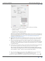
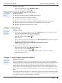
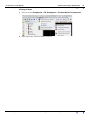
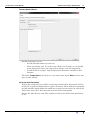
1
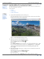
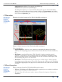
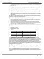
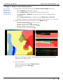
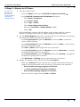
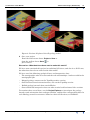
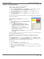
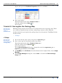
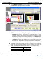
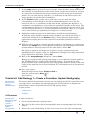
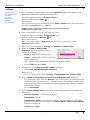
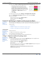
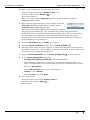
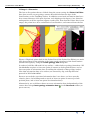
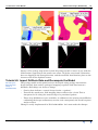
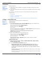
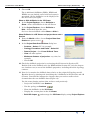
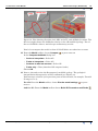
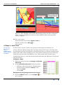
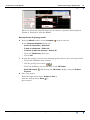
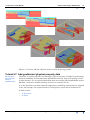
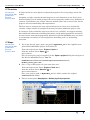
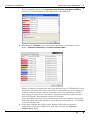
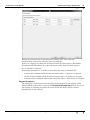
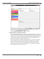
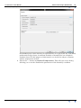
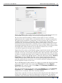
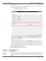
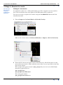
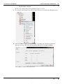
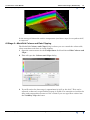
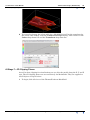
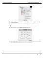
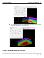
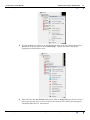
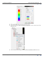
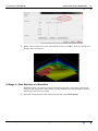
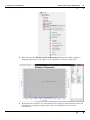
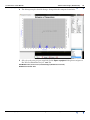
GeoModeller User Manual
Contents | Help | Top
Tutorial case study J (Geothermal)
1
| Back |
Tutorial case study J (Geothermal)
Parent topic:
User Manual
and Tutorials
This short course provides:
•
An introduction to building and updating a 3D geology model using 3D
GeoModeller.
•
A demonstration of 3D GeoModeller’s geothermal modelling capability.
Authors
Phil McInerney, Helen Gibson, Intrepid Geophysics
Updated V2012: Stewart Hore
Disclaimer
It is Intrepid Geophysics’ understanding that this tutorial document and associated
data are provided for purpose of training in the use and application of 3D
GeoModeller, and the material and data cannot be used or relied upon for any other
purpose. Intrepid Geophysics is not liable for any inaccuracies (including any
incompleteness) in this material and data.
Contents Help | Top
© 2013 BRGM & Desmond Fitzgerald & Associates Pty Ltd
| Back |
GeoModeller User Manual
Contents | Help | Top
Tutorial case study J (Geothermal)
2
| Back |
In this case study:
•
Case Study J Introduction
•
Course Structure
•
Tutorial J1: Load the HotRox 3D GeoModeller Project
•
Tutorial J2: Examine the Project Geology and the 3D Geology Model
•
Tutorial J3: Geo-register the Geology Map
•
Tutorial J4: Add Geology 1—Create a Formation, Update Stratigraphy
•
Tutorial J5: Add Geology 2—Digitise and Recompute the Model
•
Tutorial J6: Import Drillhole Data and Recompute the Model
•
Tutorial J7: Add geothermal physical property data
•
Tutorial J8: Compute geothermal solutions
•
Case Study J References
Case Study J Introduction
Parent topic:
Tutorial case
study J
(Geothermal)
In this case study we calculate the equilibrated, steady state temperature
distribution of the modelled geology in our project area. Given certain assumptions
and boundary conditions (described below), the distribution of resulting in-situ
formation temperatures is related to the 3D distribution of lithologies in our model,
and their related thermal properties (thermal conductivity and heat production rate).
At present the geothermal module accounts for heat contributions from conductivity
and internal heat production. This is considered to be adequate for many geological
settings involving ‘hot dry rock’ geothermal resources. However, improved 3D
temperature estimation will be available in the future through implementation of
advection considerations.
HotRox Project scenario
Geothermal energy company geologists have established from outcrop samples that
the HotRox Project granite has anomalously high heat-producing properties due to its
radiogenic mineralogy (heat production rate of 15 µW/m3). The granite outcrops east
of a major basin-margin fault, but interpretation of seismic and gravity data indicate
that the granite also extends further west beneath the basin sediments in the vicinity
of Section sCC. The Upper Palaeozoic unit of the basin sequence is a fine grained
shale with low thermal conductivity (1.5 W/m/K—based on analysis of samples from
drillhole DDH3 on Section sCC). This shale unit is potentially a thermal insulator.
With encouraging results from heat flow data and geothermal gradients measured in
drillhole DDH3, the company has begun a 3D geology and temperature modelling
study to:
Contents Help | Top
•
Investigate the geothermal potential of their tenement, and to
•
Estimate the total heat resource of their project ‘volume’
© 2013 BRGM & Desmond Fitzgerald & Associates Pty Ltd
| Back |
GeoModeller User Manual
Contents | Help | Top
Tutorial case study J (Geothermal)
3
| Back |
Course Structure
Parent topic:
Tutorial case
study J
(Geothermal)
This case study has two main sections:
•
Build and Revise a 3D Geology Model
•
Perform Geothermal Modelling
Build and Revise a 3D Geology Model
Parent topic:
Course
Structure
Tutorial J1: Load the HotRox 3D GeoModeller Project
We load an existing project, and examine the main elements of the user interface
Tutorial J2: Examine the Project Geology Map and the 3D Geology Model
First examine the geology map for the project, and review the project’s stratigraphic
pile. Compute the geology model. Plot the geology model in map and section views in
the 2D Viewer. Build the 3D shapes of the geology model and examine in the 3D
Viewer.
Tutorial J3: Geo-register the Geology Map
Existing geology maps and sections are easily geo-registered, and contacts digitised.
We geo-register the geology map on the TopoMap (surface) section.
Tutorial J4: Add Geology 1—Create a Formation, Update Stratigraphy
We want to add the LateGranite1 intrusive to our geology model. We must first create
a geology object, and update the stratigraphic pile.
Tutorial J5: Add Geology 2—Digitise and Recompute the Model
We can now digitise the LateGranite1 contact, and build a revised 3D geology model.
And again examine the 3D geology model in 2D and 3D views.
Tutorial J6: Import Drillhole Data and Recompute the Model
We import data for three drillholes, and project the drillhole geology onto vertical
cross-sections. Note the inconsistency between the new data and the existing 3D
model and consider the implications. Introduce a new fault to the project, compute the
new 3D geology model. Again examine the 3D geology model in 2D and 3D views.
Perform Geothermal Modelling
Parent topic:
Course
Structure
Tutorial J7: Add the Geothermal Physical Property Data
We now add geothermal physical property data for each geology unit—the thermal
conductivities and heat production rates.
Tutorial J8: Compute Geothermal Solutions
Set up boundary conditions, and compute in situ temperatures throughout the
volume of our 3D geology model. Examine the results for temperature and other
temperature-related parameters (heat flow and geothermal gradient) on selected
sections.
Contents Help | Top
© 2013 BRGM & Desmond Fitzgerald & Associates Pty Ltd
| Back |
GeoModeller User Manual
Contents | Help | Top
Tutorial case study J (Geothermal)
4
| Back |
Tutorial J1: Load the HotRox 3D GeoModeller Project
Parent topic:
Tutorial case
study J
(Geothermal)
In this tutorial we load a 3D GeoModeller project and examine the components of
the 3D GeoModeller workshops.
In the tutorial:
•
J1 Steps
•
J1 Discussion
•
J1 More information
1
Launch 3D GeoModeller from the desktop icon
J1 Steps
Parent topic:
Tutorial J1:
Load the
HotRox 3D
GeoModeller
Project
The 3D GeoModeller welcome screen appears with a main menu and toolbars
arranged across the top, left and right sides.
Figure 1. 3D GeoModeller welcome screen.
2
Open the start-point 3D GeoModeller project.
From the main menu choose Project > Open or
from the Project toolbar choose Open
or
press CTRL+O
In the Open a project dialog box navigate to the 3D GeoModeller Project .xml
file. In a typical installation this will be in C:\GeoModeller1.3.x(Build#)
\tutorial\CaseStudyJ\StartTutorialJ1\HotRox_Start_Ex1.xml
Choose Open.
3
Save your own copy of this project, so that you don’t accidentally overwrite the
original project files
From the main menu choose Project > Save as or
from the Project toolbar choose Save As
or
press CTRL+SHIFT+S.
Save your project work as MyHotRox_01 in a folder outside the original
Contents Help | Top
© 2013 BRGM & Desmond Fitzgerald & Associates Pty Ltd
| Back |
GeoModeller User Manual
Contents | Help | Top
Tutorial case study J (Geothermal)
5
| Back |
StartTutorial folder. For example, one folder up:
GeoModeller\tutorial\CaseStudyJ
Use Windows Explorer to review the files that make up the 3D GeoModeller
project. You can see that you have created a folder called MyHotRox_01, within
which are all of the files that constitute this 3D geology project. These also use the
base filename MyHotRox_01.
J1 Discussion
Parent topic:
Tutorial J1:
Load the
HotRox 3D
GeoModeller
Project
Examine the main elements of the 3D GeoModeller workspace.
Figure 2. Main elements of the 3D GeoModeller workspace.
Note in particular:
•
Project Explorer—this has a tree structure containing the many objects that
make up our 3D geology project: Formations, Faults, Models, Sections, Drillholes,
etc.
•
2D Viewer—contains 2D sections. This Tutorial J1 project contains several
sections—a special one—the ‘geological map view’ (labelled as TopoMap in this
project), and four vertical cross-sections. We use the sections for data input, and
for examining 2D plots of our 3D model.
•
3D Viewer—contains the 3D view of our project. At this stage it shows only the
bounding extents of the project. The yellow lines are the outlines of the TopoMap
section (the topography of the project area) in the 3D Viewer, and the four vertical
sections.
J1 More information
Parent topic:
Tutorial J1:
Load the
HotRox 3D
GeoModeller
Project
Contents Help | Top
Some comments about the 3D GeoModeller project space:
•
X (East), Y (North) and Z (Elevation, positive upwards) are a standard coordinate
framework according to a right-hand rule
•
X, Y and Z are all in the same units—metres (Cannot be degrees of latitude or
longitude)
© 2013 BRGM & Desmond Fitzgerald & Associates Pty Ltd
| Back |
GeoModeller User Manual
Contents | Help | Top
Tutorial case study J (Geothermal)
6
| Back |
•
X and Y would typically be real world projected coordinates, but could be a local
mine grid, etc.
•
Z is Elevation, and is positive upwards. It also would typically use a real world
vertical datum such as mean sea level
•
You can (and should) define the Projection (actually a Coordinate System,
consisting of a Datum and Projection)
•
All data must be within the project limits; data outside those limits cannot be
imported or created
•
Likewise all modelled results—geology lines, polygons and surfaces—are within
those limits
So, when you create your own project, make the project dimensions large enough to
include all geology data used in the project.
Remember to allow for the full topographic height of the project area:
•
We recommend that you leave, say, 5–10% extra space at the top of the project,
above the highest point of the topography
•
Allow sufficient project space at the bottom for the entire range of modelled
geology that you are interested in. Don’t, however, make it too large or you will
take extra time to compute model shapes that are of no interest
For this project the project dimensions and coordinate system (Datum and Projection)
are:
•
Projection—Local
•
Height Datum—Local
•
Extents
Minimum
Maximum
Range
East
50,000
90,000
40,000 m
North
100,000
140,000
40,000 m
Z-axis
–10,0000
2,000
12,000 m
The topography map view (TopoMap) in a 3D GeoModeller project is a special
(pseudo-non-planar) section, and it is an essential part of the project. You cannot do
any practical work in a 3D GeoModeller project until the map view section has been
created. Since topography defines the natural upper limit of a typical 3D geology
model, we use a digital terrain model (DTM) file to correctly define the shape of this
special TopoMap section. Using the correct topographic shape has geology mapping
advantages, and we recommend it.
If a DTM is not available, the map view section can simply be a horizontal plane at a
specified height. (We don’t recommend this. If you don’t have your own DTM,
download DTM data from the Shuttle Radar Topographic Mission website.)
Once the DTM (topography) has been loaded, and the map view section created
(called TopoMap in this project), the 3D GeoModeller project dimensions cannot be
changed.
Contents Help | Top
© 2013 BRGM & Desmond Fitzgerald & Associates Pty Ltd
| Back |
GeoModeller User Manual
Contents | Help | Top
Tutorial case study J (Geothermal)
7
| Back |
Tutorial J2: Examine the Project Geology and the 3D Geology Model
Parent topic:
Tutorial case
study J
(Geothermal)
The HotRox_Start_Ex1 3D GeoModeller Project that we have just loaded already
has a geological model of (most of) the HotRox project area.
In this section:
•
J2 Overview
•
J2 Stage 1—Compute and view the 3D model
•
J2 Stage 2—Explore model plotting options
•
J2 Stage 3—Explore the 3D Viewer
•
J2 Stage 4—Visualising drillholes
J2 Overview
Parent topic:
Tutorial J2:
Examine the
Project Geology
and the 3D
Geology Model
In this tutorial we:
1
Examine the geology map for the project, and review the Project’s stratigraphic
pile
2
Compute the geology model, and plot modelled geology in map and section views
(2D Viewer)
3
Build 3D shapes of the geology model and examine (3D Viewer)
J2 Stage 1—Compute and view the 3D model
Parent topic:
Tutorial J2:
Examine the
Project Geology
and the 3D
Geology Model
1
If it is not already open, open your project, or the supplied start-point 3D
GeoModeller project for Tutorial J1.
From the main menu choose Project > Open or
from the toolbar choose Open
or
press CTRL+O
(For the start-point project supplied) In the Open a project dialog box navigate to
the 3D GeoModeller Project .xml file
GeoModeller\tutorial\CaseStudyJ\StartTutorialJ1\
HotRox_Start_Ex1.xml
2
(If you have not already done so) Save your own copy of this project, so that you
don’t accidentally overwrite the original project files
From the main menu choose Project > Save as or
from the toolbar choose Save As
or
press CTRL+SHIFT+S.
Save your project work as MyHotRox_01 in a folder outside the original
StartTutorial folder.
Contents Help | Top
© 2013 BRGM & Desmond Fitzgerald & Associates Pty Ltd
| Back |
GeoModeller User Manual
Contents | Help | Top
3
Tutorial case study J (Geothermal)
8
| Back |
Examine the geology map and stratigraphic column (Figure 3).
Consider the rock relationships, including:
•
Cross-cutting relationships
•
Timing implications
•
Conformable sequences
From the main menu choose Geology > Stratigraphic Pile: Visualise to open the
Stratigraphic Pile Viewer.
Compare the stratigraphic pile in the 3D GeoModeller Project (Figure 4) with the
geology map. Note the important geological details that are recorded in the
stratigraphic pile (Figure 4)—the chrono-stratigraphic order of geological events,
the onlap or erode relationships, etc. You may spot that LateGranite1 in the
geology map is not yet in the model—we will add that in Tutorials J4 and J5.
4
Compute the 3D geology model for the Project that we have loaded (to be
constrained by the geological data existing within the current Project).
From the Model toolbar, choose Compute
or press CTRL+M
In the Compute the Model dialog box:
•
Series to interpolate—Select All
•
Faults to interpolate—Select All
•
Sections to take into account—Select All
•
Faults only—Clear (therefore DO compute faults)
•
Choose OK
3D GeoModeller computes the model. (Nothing to see yet.) The model is a
mathematical model—a set of interpolator equations that are computed from the
geology contacts and orientation data. There is an interpolator equation for each
series in the stratigraphic pile, and also an equation for each fault.
Figure 3. Geology map of the HotRox Project.
Contents Help | Top
© 2013 BRGM & Desmond Fitzgerald & Associates Pty Ltd
| Back |
GeoModeller User Manual
Contents | Help | Top
Tutorial case study J (Geothermal)
9
| Back |
Figure 4. Stratigraphic Pile for the HotRox (Tutorial J1) Project.
View the modelled geology
To see the modelled geology, we need to interrogate the model equations. We can:
•
Plot the modelled geology on the TopoMap 2D section (the Project’s geological
map)
•
Plot the modelled geology on any other 2D cross-section
•
Build the 3D shapes of the modelled geology, and view in the 3D Viewer
5
Select TopoMap in the 2D Viewer (click it)
6
From the Model toolbar, choose Plot the model settings
or press CTRL+D
In the Plot the model settings dialog box:
•
Check Show lines
•
Choose OK
The lines of the modelled geology are plotted on the TopoMap 2D Section (map).
7
Repeat these steps and plot the modelled geology on some of the vertical crosssections (for example, sAA).
8
Save your project
From the main menu choose Project > Save or
from the toolbar choose Save
or
press CTRL+S.
Contents Help | Top
© 2013 BRGM & Desmond Fitzgerald & Associates Pty Ltd
| Back |
GeoModeller User Manual
Contents | Help | Top
Tutorial case study J (Geothermal)
10
| Back |
J2 Stage 2—Explore model plotting options
Parent topic:
Tutorial J2:
Examine the
Project Geology
and the 3D
Geology Model
1
2
Experiment with other options in the Plot the model settings dialog box:
•
Check Show fill to plot ‘solid’ geology
•
Choose Apply to All (sections) to plot all (open) 2D sections
•
For Show lines or Show fill, select or de-select various combinations of
formations
•
Choose Show trend lines in combination with Show lines or Show fill
•
Modify the Plotting resolution from the default u=50, v=50 to, say, 100 x 100
Experiment with the three plot buttons in the Model toolbar:
•
Plot the model settings
or press CTRL+D
•
Plot the model on the current section
•
Plot the model on all sections
Figure 5. Various plots options displaying the 3D geology model on Sections
TopoMap, sAA, sBB and sCC.
3
Save your project
From the main menu choose Project > Save or
from the toolbar choose Save
or
press CTRL+S.
Contents Help | Top
© 2013 BRGM & Desmond Fitzgerald & Associates Pty Ltd
| Back |
GeoModeller User Manual
Contents | Help | Top
Tutorial case study J (Geothermal)
11
| Back |
J2 Stage 3—Explore the 3D Viewer
Parent topic:
Tutorial J2:
Examine the
Project Geology
and the 3D
Geology Model
1
View the model in 3D:
•
From the Model toolbar choose Build 3D Formations and Faults
•
In the Build 3D Formation and Fault Shapes dialog box:
•
Check Build—Formations
•
Check Build—Faults
•
Select Type—Volume
•
Check Draw Shapes after building
•
Adjust the Resolution—Render quality to High
•
Choose OK
3D GeoModeller computes the 3D shapes of the geology model as ‘volumes’
defined by triangle mesh surfaces, which it displays in the 3D Viewer.
2
Use the Project Explorer (typically on the left-side of your work space) to manage
the display of modelled objects in the 3D Viewer.
•
In the Project Explorer right-click Models > and select Hide—to hide the
entire modelled geology
•
In the Project Explorer right-click Models > and select Show—to show again
the entire modelled geology
The Hide or Show options toggle from one to the other.
•
In the Project Explorer right-click Models > and select Wireframe—to change
the displayed 3D volumes to wireframes
•
In the Project Explorer right-click Models > and select Shading—to toggle the
3D display of geology back to shaded
The Wireframe or Shading options toggle from one to the other.
3
Display the plotted geology (2D) sections in the 3D Viewer
•
With any 2D Viewer window selected (for example, sAA) from the shortcut
(right-click the background of the 2D viewer), and choose from the Menu:
•
Show modelled geology polygons in 3D Viewer
•
or, Show modelled geology lines in 3D Viewer
•
Hide modelled geology polygons in 3D Viewer
These menu items toggle between Hide and Show.
Contents Help | Top
© 2013 BRGM & Desmond Fitzgerald & Associates Pty Ltd
| Back |
GeoModeller User Manual
Contents | Help | Top
Tutorial case study J (Geothermal)
12
| Back |
Figure 6. Various 3D plots of the 3D geology model.
4
Save your project
From the main menu choose Project > Save or
from the toolbar choose Save
or
press CTRL+S.
Discussion—What data have been used to make this model?
We have now examined this project in traditional 2D views, and also in a 3D Viewer,
but what data have been used to make this model?
We have used the following geological facts and interpretive data:
•
The stratigraphic order of events and the rock relationships—both recorded in the
stratigraphic pile
•
Mapped geology contacts on the TopoMap surface section
•
Some field-measured orientation data, also on the TopoMap section
•
Drilled geology intervals from two drillholes
•
Some additional interpretive data on other vertical and horizontal slice sections
To examine these actual data, use the Project Explorer to investigate the geology
interface and orientation data catalogued within, and find the corresponding data for
each lithology stored in structures linked to either: 2D Sections, or Drillholes.
Contents Help | Top
© 2013 BRGM & Desmond Fitzgerald & Associates Pty Ltd
| Back |
GeoModeller User Manual
Contents | Help | Top
Tutorial case study J (Geothermal)
13
| Back |
J2 Stage 4—Visualising drillholes
In this section we learn about viewing drillholes.
Show and Hide drillholes in the 3D Viewer
1
First, in the Project Explorer right-click Models > and select Hide—to hide the
entire modelled 3D geology (so the drillholes will be visible)
2
In the Project Explorer, right-click Drillholes > and select Show—shows all
drillholes in the 3D Viewer
3
In the Project Explorer, right-click Drillholes > and select Hide—hides them
again from the view
You can also show or hide individual drillholes, by first expanding the list of drillholes
in the Project Explorer.
Show drillholes in a 2D Viewer (Project them onto a
Section)
1
From the Model toolbar, choose Project Data Onto
Sections
or press CTRL+I
2
In the Project Data Onto Sections dialog box
•
Geology Formations and Faults—Select All
•
Sections—Select sCC, for example
•
Data to project—Check from Drillhole Trace
•
Clear all other check boxes
•
Maximum distance of projection—try 10m, for example
•
Choose OK
The trace of HRW2 can now be seen in the 2D Viewer for sCC, because the drillhole is
located less than 10m off that section.
Now examine the geology intervals in a drillhole using drillhole properties
Either:
In the Project Explorer, choose and expand Drillholes > (select a Drillhole name) >
click Properties. This opens the Drillhole Properties table for a drillhole, showing the
downhole depths and the intersected geology for each interval.
Alternatively:
Contents Help | Top
1
From the 2D toolbar, choose Select
or press S
2
Make sure Project Data Onto Sections is shown for at least one drillhole, on at
least one section, as explained above.
3
Double click on any projected drillhole trace or triangle symbol in a section in the
2D Viewer
© 2013 BRGM & Desmond Fitzgerald & Associates Pty Ltd
| Back |
GeoModeller User Manual
Contents | Help | Top
Tutorial case study J (Geothermal)
14
| Back |
Again, this opens the Drillhole Properties table for a drillhole:
4
Save your project
From the main menu choose Project > Save or
from the toolbar choose Save
or
press CTRL+S.
Tutorial J3: Geo-register the Geology Map
Parent topic:
Tutorial case
study J
(Geothermal)
Existing geology maps and sections are an important source of geology data. These
are easily geo-registered onto sections, and geology contacts can be digitised.
In this tutorial we geo-register the geology map on to the project’s TopoMap Section.
In this section:
•
J3 Steps
1
If it is not already open, open your project MyHotRox_01.
2
Save a new copy of your project with a new name
J3 Steps
Parent topic:
Tutorial J3:
Geo-register the
Geology Map
From the main menu choose Project > Save as or
from the toolbar choose Save As
or
press CTRL+SHIFT+S.
In the Save the project dialog box, change the name from MyHotRox_01 to
MyHotRox_03 and then choose Save.
Contents Help | Top
3
In TopoMap in the 2D Viewer, from the shortcut menu (right click), choose Image
Manager.
4
In the Image Manager dialog box, choose New... to launch the Edit and Align
Image tool.
© 2013 BRGM & Desmond Fitzgerald & Associates Pty Ltd
| Back |
GeoModeller User Manual
Contents | Help | Top
5
Tutorial case study J (Geothermal)
15
| Back |
From the Edit and Align Image tool, browse to the image file CaseStudyJ\Data\
HotRoxProject_Geology.png. Select and Open.
Figure 7. Geo-registration of the geology map image onto the TopoMap section.
The Edit and Align Image tool displays the image in two windows:
6
Contents Help | Top
•
An Image display on the left, which operates in terms of the image’s (i, j) pixel
coordinates. There are three moveable image markers on this display, which
are linked one-to-one to corresponding section markers of the Section display
(on the right). The (i, j) coordinates of the three image markers are tabled
below the display.
•
A Section display on the right, which operates in terms of the section’s (u, v)
coordinate space. There are three moveable section markers on the display.
The (u, v) coordinates and corresponding (x, y, z) coordinates of the three
section markers are tabled below the display.
Examine the image, and note that the map corners can be used as geo-registration
marks, since these have known coordinates. Press the magnifier icon to zoom, and
use the two sliders to pan horizontally or vertically to read the map corner
coordinates (tabled below).
Bottom or Left
Top or Right
East
50,000
90,000
North
100,000
140,000
© 2013 BRGM & Desmond Fitzgerald & Associates Pty Ltd
| Back |
GeoModeller User Manual
Contents | Help | Top
Tutorial case study J (Geothermal)
16
| Back |
7
In the Image display (pale blue area, left side), move the three image markers to
three known geo-registration marks on the image. Progressively zoom in, and pan
to each mark, and position the image markers precisely on the geo-registration
marks. You can also directly edit the (i, j) coordinates in the table to move the
image markers to specific pixel coordinates.
8
In the Section display (yellow area, right side), you can move the three
corresponding section markers, but the recommended practice is to edit the
entries for the (u, v) coordinates in the table below, inputting the known (u, v)
coordinates corresponding to each of the geo-registration marks on the image. The
section markers will move as you do this. Again, zoom and pan if you want to. You
can also directly edit the (x, y, z) real coordinates in the table. (This (x, y, z) option
can be useful when geo-registering an image on a vertical section).
9
Additional marker points can be added (they are added to both displays).
As both the image markers and the section markers are moved, the image is
continually ‘distorted’ in the Section display, illustrating the proposed georegistration warping based on the current set of marker positions on the two
displays.
10 With the image markers correctly placed precisely on the known geo-registration
marks on the Image (left), and the known coordinates corresponding to each of the
section markers correctly entered in the table below, choose OK.
The image is warped, and clipped as required, and geo-registered onto the
TopoMap Section. As this occurs, an “Information” dialogue box with transformed
image dimensions will show. Choose OK.
11 Back in the Image Manager dialog box, choose Close.
Having geo-registered the geology map image, you can plot the current model on
the TopoMap Section. Compare the modelled geology—as developed to this
point—with the map. Notice that the late-stage granite intrusive in the south-east
corner of the map has not yet been modelled. We will add that unit in Tutorials J4
and J5.
12 Save your project
From the main menu choose Project > Save or
from the toolbar choose Save
or
press CTRL+S.
Tutorial J4: Add Geology 1—Create a Formation, Update Stratigraphy
Parent topic:
Tutorial case
study J
(Geothermal)
We want to add the LateGranite1 intrusive to our geology model. We must first create
a geology object, and update the stratigraphic pile. In Tutorial J5 we digitise the
LateGranite1 contact, and build the revised 3D geology model.
In this section:
•
J4 Overview
•
J4 Steps
J4 Overview
Parent topic:
Tutorial J4: Add
Geology 1—
Create a
Formation,
Update
Stratigraphy
Contents Help | Top
In this tutorial we:
1
Create the LateGranite1 geology object
2
Place this in the correct chrono-stratigraphic order in stratigraphic pile for the
Project
3
Declare the rock relationship. In this case it cuts across the older stratigraphy
© 2013 BRGM & Desmond Fitzgerald & Associates Pty Ltd
| Back |
GeoModeller User Manual
Contents | Help | Top
Tutorial case study J (Geothermal)
17
| Back |
J4 Steps
Parent topic:
Tutorial J4: Add
Geology 1—
Create a
Formation,
Update
Stratigraphy
1
If it is not already open, open your project MyHotRox_03 or the supplied startpoint 3D GeoModeller project for Tutorial J4.
From the main menu choose Project > Open or
from the toolbar choose Open
or
press CTRL+O
(For the start-point project supplied) In the Open a project dialog box navigate to
the 3D GeoModeller Project .xml file
GeoModeller\tutorial\CaseStudyJ\StartTutorialJ4\
HotRox_Start_Ex4.xml
2
Save a copy of this project in your own data area.
From the main menu choose Project > Save as or
from the toolbar choose Save As
or
press CTRL+SHIFT+S.
Save your project work as MyHotRox_04 in a folder outside the original
StartTutorial folder.
3
From the main menu choose Geology > Formations: Create or Edit
4
From the Create or Edit geology
formations dialog box (Create a new
geology formation):
5
•
Name—LateGranite1 (No spaces!)
•
Colour—(pink (RGB = 255,20,147) used
in this document)
•
Note: Many geology formations already exist in this project.
•
Choose Add and then Close
If prompted, in the New formation creation dialog box:
•
Choose Yes, start Stratigraphic Pile editor
Alternatively:
•
6
7
Contents Help | Top
From the main menu choose Geology > Stratigraphic Pile: Create or Edit
In the Create or Edit geology series and the stratigraphic pile dialog box:
•
For future reference, note that Bottom is the chosen option; for this project we
model ‘bottoms’ of formations (i.e., all data entered is assumed to relate to the
chronologically, bottom-boundary of the given geology unit, where it contacts
with the unit below).
•
Choose New series
In the Create Geology Series dialog box, confirm default entries, or change the
following to:
•
Name of the series—LateGranite1_Series
•
Relationship—Erode
•
Formations in Series—LateGranite1 (Ensure this formation is in the rightside list. Select formation(s) and use the Add to Series or Remove from Series
buttons as required)
•
Commit then Close
© 2013 BRGM & Desmond Fitzgerald & Associates Pty Ltd
| Back |
GeoModeller User Manual
Contents | Help | Top
8
9
Tutorial case study J (Geothermal)
18
| Back |
Back in the Create or Edit geology series and the stratigraphic pile dialog box:
•
Check that the series are in the correct
stratigraphic order, with this late-stage
granite intrusive placed towards the top of
the list, above the Mafic Dyke and below the
LateGranite2 (select the new series, and use
the Move up and Move down buttons as
required).
•
Then Close
From the main menu choose Geology > Stratigraphic Pile: Visualise
10 In the Stratigraphic Pile Viewer dialog box, review and then Close
11 Save your project
From the main menu choose Project > Save or
from the toolbar choose Save
or
press CTRL+S.
Tutorial J5: Add Geology 2—Digitise and Recompute the Model
Parent topic:
Tutorial case
study J
(Geothermal)
Having created a geology object, and updated the stratigraphic pile in Tutorial J4, we
can now digitise the LateGranite1 contact, and build a revised 3D geology model.
In this section:
•
J5 Overview
•
J5 Stage 1—Digitise the LateGranite1 geology contact
•
J5 Stage 2—Recompute and visualise in 2D and 3D
J5 Overview
Parent topic:
Tutorial J5: Add
Geology 2—
Digitise and
Recompute the
Model
In this tutorial we:
1
Digitise the LateGranite1 geology contact
2
Recompute the 3D geology model
3
Again examine the 3D geology model in 2D and 3D views
J5 Stage 1—Digitise the LateGranite1 geology contact
Parent topic:
Tutorial J5: Add
Geology 2—
Digitise and
Recompute the
Model
J5 Stage 1—Steps
1
If it is not already open, open your project MyHotRox_04 or the supplied startpoint 3D GeoModeller project for Tutorial J5.
From the main menu choose Project > Open or
from the toolbar choose Open
or
press CTRL+O
(For the start-point project supplied) In the Open a project dialog box navigate to
the 3D GeoModeller Project .xml file
GeoModeller\tutorial\CaseStudyJ\StartTutorialJ5\
HotRox_Start_Ex5.xml
Contents Help | Top
© 2013 BRGM & Desmond Fitzgerald & Associates Pty Ltd
| Back |
GeoModeller User Manual
Contents | Help | Top
2
Tutorial case study J (Geothermal)
19
| Back |
Save a copy of this project in your own data area.
From the main menu choose Project > Save as or
from the toolbar choose Save As
or
press CTRL+SHIFT+S.
Save your project work as MyHotRox_05 in a folder outside the original
StartTutorial folder.
3
Show the geo-registered image of the geology. From the
2D Viewer, TopoMap section shortcut menu, choose
HotRoxProject_Geology_t1.gif
Note the granite body mapped in the south-east corner of
the project area, labelled ‘g1’. We will model this granite as LateGranite1.
In Tutorial J4 we created the LateGranite1 geology object. We are now ready to
use that object when digitising a few contact data points along the granite
boundary. We also want create some orientation data to define that contact as
steeply dipping to the south-east.
4
From the 2D toolbar, choose Create
5
From the Points List Editor toolbar, choose Delete all Points
6
Starting at the north-east end, click five or six points along the contact between
the granite labelled ‘g1’, and the Miocene unit in dark yellow, located in the southeast corner of the geology map (Figure 8).
7
From the Structural toolbar choose Create geology data
8
In the Create geology data dialog box:
9
or press C
or press CTRL+G
•
Geological Formations and Faults—select LateGranite1
•
This dialog box allows us to create some associated orientation data, too—
these are orientation data created between each pair of digitised data points.
•
Check on Associated
•
Select Dip constant, and set Dip = 80 (degrees)
•
Polarity—select Normal
•
Choose Create, and then Close
Save your project
From the main menu choose Project > Save or
from the toolbar choose Save
or
press CTRL+S.
Contents Help | Top
© 2013 BRGM & Desmond Fitzgerald & Associates Pty Ltd
| Back |
GeoModeller User Manual
Contents | Help | Top
Tutorial case study J (Geothermal)
20
| Back |
J5 Stage 1—Discussion
The four or five points that we clicked along the contact using the Points List Editor
have been used to create geology contact data which define the edge of the
LateGranite1 at the TopoMap surface. In addition, associated orientation data have
been created between each pair of points, each dipping at 80 degrees, in a direction
orthogonal to each line segment (approx. south-east). Note that the Points List is now
empty; the points have been committed to LateGranite1, and removed from the list.
Figure 8. Digitised points (left) in the Points List (of the Points List Editor) are made
into ‘observations’ of the position of the lower contact (geology) of the LateGranite1
(middle and right) by using the Create geology data dialog box.
In order to build the 3D model of any surface—either fault or geology formation—3D
GeoModeller requires at least one point of contact (or fault position) data, and at
least one point of orientation data, describing the attitude of that geology surface.
Note that orientation data (of a surface) are entered by ‘dip, and dip-direction’
protocol in 3D GeoModeller.
Because we used the ‘associated orientation data’ case above, we have met the
criteria, above, for building surfaces (need at least one point of contact [or fault
position] data, and at least one point of orientation data).
Alternatively, we could have chosen to create orientation data independently of the
contact data using Create geology orientation data
in the Structural toolbar (or
press CTRL+R).
Contents Help | Top
© 2013 BRGM & Desmond Fitzgerald & Associates Pty Ltd
| Back |
GeoModeller User Manual
Contents | Help | Top
Tutorial case study J (Geothermal)
21
| Back |
J5 Stage 2—Recompute and visualise in 2D and 3D
Parent topic:
Tutorial J5: Add
Geology 2—
Digitise and
Recompute the
Model
J5 Stage 2—Steps
1
From the Model toolbar, choose Compute
2
In the Compute the Model dialog box:
3
or press CTRL+M
•
Note that a new series—the LateGranite1—is now available to be computed:
•
Clear the ‘Faults only’ box
•
Series to interpolate—Select All
•
Faults to interpolate—Select All
•
Sections to take into account—Select All
•
Choose OK
From the Model toolbar, choose from the available plotting options
•
Plot the model settings
or press CTRL+D
•
Plot the model on the current section
•
Plot the model on all sections
Repeat these steps, choosing different options to plot the geology model in
different ways on one or more of the sections.
4
From the Model toolbar, choose Build 3D Formations and Faults
Visualise the revised geology model in the 3D Viewer. Use the Project Explorer to
Show or Hide different formations or units of the 3D geology model.
5
Save your project
From the main menu choose Project > Save or
from the toolbar choose Save
or
press CTRL+S.
J5 Stages 1 and 2—Discussion
Did your revision produce the expected granite body in the south-east corner of the
project area? To check this you need to plot ‘solid geology’ rather than ‘lines’, and
compare your result with Figure 9, below.
If your solid geology map looks like Figure 9a, your 3D geology model is correct; the
LateGranite1 body is a 3D body in the south-east corner of the project.
If your map looks like Figure 9b:
•
what has gone wrong?
•
how did this happen?
•
how do you fix it?
What has gone wrong?
Essentially the problem is the ‘facing direction’ of the geology boundary that you
created to model LateGranite1. If you look closely at the ‘associated orientation data’
that we created, you will see that—for the incorrect case—the dips are steeply
dipping towards the north-west (Figure 9b). This is also the ‘facing’ direction, and, as
a result, the modelled LateGranite1 body lies to the north-west side of the digitised
contact.
Contents Help | Top
© 2013 BRGM & Desmond Fitzgerald & Associates Pty Ltd
| Back |
GeoModeller User Manual
Contents | Help | Top
Tutorial case study J (Geothermal)
22
| Back |
How did this happen?
At Step 6 of Stage 1 (above) we stated “Starting at the north-east end, click four to
five points along the contact”. The key point is ‘Starting at the north-east end’. In
creating ‘associated orientation data’ with a constant dip of 80 degrees—as we did in
Step 8 of Stage 1—those orientation data are generated to be dipping in a direction
which is locally orthogonal to each line-segment of the digitised line—and to the left.
If you digitised the line starting at the north-east end and working towards the
southern end, then ‘left’ would be ‘towards the south-east’, which would be correct.
But, if you digitised the line in the other direction—starting at the southern end—
then ‘left’ would be ‘towards the north-west’, yielding the wrong result.
How do you fix this?
This small problem is easily fixed.
1
Move the mouse pointer over the LateGranite1 digitised data points and right
click to open the shortcut menu
2
Choose Flip associated dip direction
The ‘associated dips’ will be changed to now dip at 80 degrees towards the south-east.
When the model is re-computed and re-plotted, the modelled geology map will now be
correct, as shown in Figure 9a.
Remember, the alternative method of adding orientation data (slower, but perhaps
more fool-prove) is not to use the ‘associated orientation data’ method, but the
independent method: From the 2D toolbar, choose Create
or press C. Digitise two
points in the approximate position along the strike-direction of the dipping surface. In
the Structural toolbar choose Create geology orientation data
(or press CTRL+R).
In the Create geology orientation data dialog box:
Geological Formations and Faults—select LateGranite1
Direction—select dip direction=105 degrees, and select Dip=80 degrees
Polarity=Normal. Choose Create and Close.
Contents Help | Top
© 2013 BRGM & Desmond Fitzgerald & Associates Pty Ltd
| Back |
GeoModeller User Manual
Contents | Help | Top
Tutorial case study J (Geothermal)
23
| Back |
Figure 9. The geology map of the revised 3D geology model is correct in (a), with the
LateGranite1 appearing in the south-east corner. In (b) the ‘associated’ orientation
data are dipping in the wrong direction, and the modelled LateGranite1 plots on the
incorrect side of the digitised contact.
Tutorial J6: Import Drillhole Data and Recompute the Model
Parent topic:
Tutorial case
study J
(Geothermal)
The geology model at this point has been developed using geology observations
derived mainly from surface geological mapping, together with data from two
drillholes. But things are about to change.
•
Gravity data indicate a central, deeper basin—a graben?
•
Towards the north-west, field mapping shows evidence for a fault. This is
interpreted to lie along the western edge of a postulated graben.
•
Three deep drillholes are now available, in addition to the existing two drillholes,
confirming the deeper sedimentary section, and consequently the model requires
major revision.
Change is easily implemented in 3D GeoModeller. Let’s now make the changes.
Contents Help | Top
© 2013 BRGM & Desmond Fitzgerald & Associates Pty Ltd
| Back |
GeoModeller User Manual
Contents | Help | Top
Tutorial case study J (Geothermal)
24
| Back |
J6 Overview
Parent topic:
Tutorial J6:
Import
Drillhole Data
and Recompute
the Model
In this tutorial we:
1
Import data for three drillholes, and project the drillhole geology onto vertical
cross-sections
2
Note and respond to discrepancy between the new drillhole data and the existing
3D model
3
Introduce a new fault to the project, and recompute the 3D geology model
In this section:
•
J6 Overview
•
J6 Stage 1—Add drillhole data
•
J6 Stage 2—Add a fault
•
J6 Stage 3—Consideration of the Proterozoic offset by the Western Fault
J6 Stage 1—Add drillhole data
Parent topic:
Tutorial J6:
Import
Drillhole Data
and Recompute
the Model
In this stage we add and examine the drillhole data
Load the project
1
If it is not already open, open your project MyHotRox_05 or the supplied startpoint 3D GeoModeller project for Tutorial J6.
From the main menu choose Project > Open or
from the toolbar choose Open
or
press CTRL+O
(For the start-point project supplied) In the Open a project dialog box navigate to
the 3D GeoModeller Project .xml file
GeoModeller\tutorial\CaseStudyJ\StartTutorialJ6\
HotRox_Start_Ex6.xml
2
Save a copy of this project in your own data area.
From the main menu choose Project > Save as or
from the toolbar choose Save As
or
press CTRL+SHIFT+S.
Save your project work as MyHotRox_06 in a folder outside the original
StartTutorial folder.
Load the drillhole data
Contents Help | Top
3
From the main menu choose Import > Import Drillhole Data > Import Collars,
Surveys, Geology (3 files)
4
In the Load Drillhole CSV dataset dialog box:
•
Browse to the ‘Collar Table’ file (HotRox_DDH_Collars.csv in the
CaseStudyJ\Data\ folder) and then use the drop-down lists of labelled
‘columns’ to assign the correct file columns to the fields required by 3D
GeoModeller—the drillhole’s Hole ID, its (X, Y, Z) collar coordinate and the
Hole Depth.
•
Similarly, browse to the ‘Survey Table’ file and assign the correct file columns
to the required fields.
•
Similarly, browse to the ‘Geology Table’ file and assign the correct file columns
to the required fields.
© 2013 BRGM & Desmond Fitzgerald & Associates Pty Ltd
| Back |
GeoModeller User Manual
Contents | Help | Top
5
Tutorial case study J (Geothermal)
25
| Back |
Choose OK
The 3 additional drillholes (DDH1, DDH2 and
DDH3) are now loaded, and a brief load report is
presented. All five drillholes can be displayed in
the 3D Viewer (see right).
Show or Hide drillholes in the 3D Viewer
6
In the Project Explorer, choose Drillholes >
Show—shows all drillholes in the 3D Viewer
7
In the Project Explorer, choose Drillholes >
Hide—hides them from the view
Or, for a chosen drillhole either Show or Hide it
Show Drillholes in a 2D Viewer and project them onto a
Section
8
From the Model toolbar, choose Project Data Onto
Sections or press CTRL+I
9
In the Project Data Onto Sections dialog box:
•
Sections—Select sCC, for example
•
Geology Formations and Faults—Select All
•
Data to Project—check from Drillhole Trace
•
Clear all other options
•
Maximum distance of projection—try 10m, for
example
•
Choose OK
10 Check the drillhole projection by activating the 2D viewer for Section sCC.
Double-click on the drillhole trace for DDH3 within Section sCC (it’s the deepest
one, furthest east) to reveal the drillhole properties, including the table of geology
contacts.
11 Next, let’s examine the drillhole data relative to the original 3D geology model.
Examine these by plotting and visualising the 5 drillholes in 2D (Section) and 3D
(Viewer). Consider the interpretive changes that you need to make to best
accommodate the new drillhole data (Figure 10).
Use the same plotting options that we have used previously.
Contents Help | Top
•
Project the drillholes onto Sections
•
Plot the geology on Sections
•
Show the drillholes in the 3D Viewer
•
Display the section plots in the 3D Viewer
•
Build 3D shapes
and manage the 3D Viewer display using Project Explorer
© 2013 BRGM & Desmond Fitzgerald & Associates Pty Ltd
| Back |
GeoModeller User Manual
Contents | Help | Top
Tutorial case study J (Geothermal)
26
| Back |
Figure 10. Plan showing Sections sAA, sBB, and sCC, and drillhole locations. The
3D view (right) shows the drillholes relative to the 3D modelled geology. Two of
the new drillholes show a much deeper sedimentary section.
Now let’s recompute the model so that all 5 drill holes are taken into account.
12 From the Model toolbar, choose Compute
or press CTRL+M
In the Compute the Model dialog box:
•
Series to interpolate—Select All
•
Faults to interpolate—Select All
•
Sections to take into account—Select All
•
Faults only—Clear (therefore DO compute faults)
Choose OK
13 Now re-plot and review the Recomputed, modelled geology. The geological
interpretation-discrepancies will be confirmed (see Figure 10).
Perform steps as before (as in previous parts of this tutorial, for example, Tutorial
J2 stages 1 to 3):
For 2D: From the Model toolbar, choose Plot the model settings
CTRL+D
or press
And for 3D: From the Model toolbar choose Build 3D Formations and Faults
Contents Help | Top
© 2013 BRGM & Desmond Fitzgerald & Associates Pty Ltd
| Back |
GeoModeller User Manual
Contents | Help | Top
Tutorial case study J (Geothermal)
27
| Back |
Figure 11. The TopoMap and Section sBB showing geology for the recomputed
model. A fault is proposed to achieve a model which is more consistent with
surface mapping.
14 Save your project
From the main menu choose Project > Save or
from the toolbar choose Save
or
press CTRL+S.
J6 Stage 2—Add a fault
Parent topic:
Tutorial J6:
Import
Drillhole Data
and Recompute
the Model
In this section, we add a fault to the geology model (proposed in Figure 11).
In fact a Western Fault geology object already exists in the Project, and some data
describing the position and attitude of the Western Fault are already included in the
north-west corner of the TopoMap section. This fault currently does not exist in the
model because the fault is not linked to any of the geology series in the Project.
Considering Figure 11, note that the proposed fault offsets the Basement, Proterozoic
and Basin series.
J6 Stage 2—Steps
1
From the main menu choose Geology > Link faults
with series
2
In the Link faults with series dialog box (table):
•
Click the cells of the table to link Basement,
ProterozoicUC and Basin (Series) to the
Western (Fault)
•
Choose OK
Recompute the 3D geology model for the Project
3
Contents Help | Top
From the Model toolbar, choose Compute
press CTRL+M
or
© 2013 BRGM & Desmond Fitzgerald & Associates Pty Ltd
| Back |
GeoModeller User Manual
Contents | Help | Top
4
Tutorial case study J (Geothermal)
28
| Back |
In the Compute the Model dialog box:
•
Series to interpolate—Select All
•
Faults to interpolate—Select All
•
Sections to take into account—Select All
•
Clear the Faults only check box
•
Choose OK
J6 Stages 2—Discussion
When we try to compute the model at this point, we get a message saying ‘unable to
solve ProterozoicUC’. We examine this in the following stage.
J6 Stage 3—Consideration of the Proterozoic offset by the Western Fault
Parent topic:
Tutorial J6:
Import
Drillhole Data
and Recompute
the Model
In this section we find that we need to add some interpretive contact data for the
(bottom of) Proterozoic. We know that this contact must be beneath the two deep
basin drillholes.
J6 Stage 3 Having enough information about the geology horizon
As noted above, when we try to compute the model at this point, we get a message
saying ‘unable to solve ProterozoicUC’ series.
The reason for this is that we do not have enough information about this geology
horizon, particularly within the ‘model compartment’ created by the new fault.
Consider the following:
To the west of the Western Fault:
•
There is some outcrop of Proterozoic which provides information about the top of
the unit; the interpolator for the ProterozoicUC cannot use that information
because it relates to a different horizon. Recall that you are modelling ‘bottoms’ of
formations, not ‘tops’.
•
Three drillholes penetrated the Proterozoic and intersected the Basement—thus
providing three geology contact data points for the bottom of the Proterozoic,
which can be used by the ProterozoicUC series interpolator.
•
You can see that an orientation data point occurs on Section sAA, describing the
ProterozoicUC as dipping 5º to the east. This is also used by the ProterozoicUC
series interpolator.
These data—some contact and orientation data—provide sufficient information on
the western side of the newly proposed fault—sufficient to satisfy the needs of the
mathematical solver for the ProterozoicUC series.
To the east of the Western Fault:
Contents Help | Top
•
There is no outcrop of Proterozoic
•
Two deep (central) drillholes intersected the top of the Proterozoic
© 2013 BRGM & Desmond Fitzgerald & Associates Pty Ltd
| Back |
GeoModeller User Manual
Contents | Help | Top
Tutorial case study J (Geothermal)
29
| Back |
This is the problem. We have postulated that the Western Fault produces an offset
to the Proterozoic but we have no data to the east of the fault that says anything
about where the bottom of the down-faulted of Proterozoic unit is. The mathematical
solver cannot solve this. You, the interpreting geologist, either have to find the
required data (shoot some seismic? Expensive!) or interpret (geologists are paid to
interpret geology!)
J6 Stage 3 What do we know about the Proterozoic?
From three drillholes in the west we know the thickness of Proterozoic:
•
2641m in drillhole HRW1
•
2735m in drillhole HRW2
•
2525m in drillhole DDH1
In the two deeper ‘basin’ drillholes we know the depth to the top of the Proterozoic:
•
5350m in drillhole DDH2
•
6405m in drillhole DDH3
J6 Stage 3—The solution—adding interpretive contact data
On the basis of this information, we can reasonably estimate that the bottom of the
Proterozoic is some 2600m below the points where the top of Proterozoic was
intersected in drillholes DDH2 and DDH3. Lets add one interpretive geology contact
data point for Proterozoic on the Section sBB—below DDH2.
1
In the 2D Viewer, select Section sBB
2
Project the drillhole traces onto this section (use the Project tool
3
From the 2D toolbar, choose Tape Measure (the Tape Measure tool
)
)
Using the Tape Measure tool, click near the bottom of DDH2 in Section sBB, and
drag downwards until the measured distance in the Tape Measure dialog box
shows approximately 2600m (Figure 12).
Note the approximate position, or read off the Z-elevation value from the mouse
coordinates displayed at the lower left edge of the 2D Viewer
Create the contact data point
4
Change the mouse mode to Create. From the 2D toolbar, choose Create
press C.
or
From the Points List Editor toolbar, choose Delete all Points
Click to place a single ‘point’ at the interpreted bottom of Proterozoic beneath
DDH2
5
From the Structural toolbar, choose Create geology data
or press CTRL+G.
In the Create geology data dialog box:
Contents Help | Top
•
Geological Formations and Faults—Choose Proterozoic
•
Choose Create—You have created a single interpreted geology contact data
point for the bottom of Proterozoic.
© 2013 BRGM & Desmond Fitzgerald & Associates Pty Ltd
| Back |
GeoModeller User Manual
Contents | Help | Top
Tutorial case study J (Geothermal)
30
| Back |
Figure 12. Using the Tape Measure tool to estimate a position for interpreted
‘bottom of Proterozoic’ beneath DDH2.
Recompute the 3D geology model
6
From the Model toolbar, choose Compute
or press CTRL+M
In the Compute the Model dialog box:
7
8
•
Series to interpolate—Select All
•
Faults to interpolate—Select All
•
Sections to take into account—Select All
•
Clear the Faults only check box
•
Choose OK
Re-plot the geology. Use the same plotting options that we have used previously.
•
Project the drillholes onto sections
•
Plot the geology on sections
•
Show the drillholes and section plots in the 3D Viewer
•
Build 3D shapes
Explorer
and manage the 3D Viewer display using the Project
Save your project
From the main menu choose Project > Save or
from the toolbar choose Save
or
press CTRL+S.
Contents Help | Top
© 2013 BRGM & Desmond Fitzgerald & Associates Pty Ltd
| Back |
GeoModeller User Manual
Contents | Help | Top
Tutorial case study J (Geothermal)
31
| Back |
Figure 13. Various 2D and 3D plots of the revised 3D geology model.
Tutorial J7: Add geothermal physical property data
Parent topic:
Tutorial case
study J
(Geothermal)
Tutorials J7 and J8 take the user through a typical sequence of tasks for performing
forward modelling of 3D temperature distribution directly from a 3D geology model.
In this instance, we are forward modelling from an existing 3D GeoModeller project
(HotRox_) which we modified during exercises in tutorials J1–J6.
It is also possible to perform forward temperature modelling starting from a supplied
voxet, for example, one exported from a GoCad project (steps not described here).
In this section:
Contents Help | Top
•
J7 Overview
•
J7 Steps
© 2013 BRGM & Desmond Fitzgerald & Associates Pty Ltd
| Back |
GeoModeller User Manual
Contents | Help | Top
Tutorial case study J (Geothermal)
32
| Back |
J7 Overview
Parent topic:
Tutorial J7: Add
geothermal
physical
property data
In this tutorial we enter physical (thermal) properties for each geology unit in the
model.
Assigning a single constant thermal property to each formation is not ideal, given
that knowledge of real-world geology tells us heterogeneity within every formation is
common. Nonetheless, the current software module takes only a mean value for the
purpose of forward modelling 3D temperatures.
The best way to estimate the most representative mean value is to statistically
consider a large number of samples from many locations within the project area.
If estimates of the variability (spread of values) are available, we suggest entering
this additional information (standard deviation, multi-modal population statistics),
because future innovations potentially planned for 3D GeoModeller may use these
in estimating uncertainty in 3D temperature modelling, and / or performing
inversion.
J7 Steps
Parent topic:
Tutorial J7: Add
geothermal
physical
property data
1
If it is not already open, open your project MyHotRox_06 or the supplied startpoint 3D GeoModeller project for Tutorial J7.
From the main menu choose Project > Open or
from the toolbar choose Open
or
press CTRL+O
(For the start-point project supplied) In the Open a project dialog box navigate to
the 3D GeoModeller Project .xml file
GeoModeller\tutorial\CaseStudyJ\StartTutorialJ7\
HotRox_Start_Ex7.xml
2
Save a copy of this project in your own data area.
From the main menu choose Project > Save as or
from the toolbar choose Save As
or
press CTRL+SHIFT+S.
Save your project work as MyHotRox_07 in a folder outside the original
StartTutorial folder.
3
Contents Help | Top
Choose menu option Geophysics > Define physical properties.
© 2013 BRGM & Desmond Fitzgerald & Associates Pty Ltd
| Back |
GeoModeller User Manual
Contents | Help | Top
Tutorial case study J (Geothermal)
33
| Back |
3D GeoModeller displays the Physical properties of a geological formation
dialog box. Four tabs appear in the upper part of the dialog box.
4
Drop down the Thermal menu. Two thermal properties are available in this
menu—Thermal Conductivity and Heat Production Rate.
Firstly, for thermal conductivities note that default values of 2 W/(mK) have been
assigned to all sedimentary units, and values of 3 W/(mK) have been assigned to
all igneous and basement rocks. (It is possible, if you are continuing to modify
your own project from before Tutorial J7, that the LateGranite1 unit only has a
value of 2 W/(mK). This should be edited to 3 W/(mK).)
Your exploration team has direct measurements from core samples of the Upper
Palaeozoic (shale) that this unit has a mean thermal conductivity of ~ 1.5 W/(mK),
so we will edit this now.
5
Contents Help | Top
Scroll down through the geology units. Double click within the thermal
conductivity cell for the ‘UPalaeozoic’ unit. This will open the Thermal
Conductivity dialog.
© 2013 BRGM & Desmond Fitzgerald & Associates Pty Ltd
| Back |
GeoModeller User Manual
Contents | Help | Top
Tutorial case study J (Geothermal)
34
| Back |
Note this dialog box (below) contains a number of features including:
•
Parameters to define the distribution
•
Number of modes
•
Proportions (if more than one mode)
•
Statistical ‘law’ or distribution type
However, as noted above, the module takes only the mean value for the purpose of
forward modelling 3D temperatures. (Tools for the inversion of potential field data
adopt these distributions, see Tutorial case study E (Forward and inverse
modelling of potential field data))
6
Change the mean value to 1.5, ignoring all other entries for now. Close with the
OK button to go back to the‘physical properties of geological formation’ dialog.
7
Next, for heat production rates note that a default value of 1 µW/m3 has been
assigned to all units. However, we now have direct measurements indicating that
the ‘granite’ unit should instead be assigned a heat production rate of ~15 µW/m3,
so we edit this now.
8
Scroll back up through the geology units. Double click within the heat production
rate cell for the ‘granite’ unit, and change the mean value to 15 µW/m3.
Note you may enter this value in a number of ways depending which units you
wish to display in the right-hand cell of the Parameters dialogue box (for example,
enter 0.000015 if “ W/m3 “ units are selected rather than µW/m3).
9
Now, close this dialog box for granite. Choose OK, which saves your edits and
returns you to the Thermal menu of the physical properties table.
10 Now close ‘physical properties of geological formation’ dialogue box. Choose OK
Contents Help | Top
© 2013 BRGM & Desmond Fitzgerald & Associates Pty Ltd
| Back |
GeoModeller User Manual
Contents | Help | Top
Tutorial case study J (Geothermal)
35
| Back |
11 Save your project
From the main menu choose Project > Save or
from the toolbar choose Save
Tutorial J8: Compute geothermal solutions
Parent topic:
Tutorial case
study J
(Geothermal)
In this tutorial we:
1
Run the Geothermal Forward Modelling Wizard
2
Set model parameters using the wizard
3
Visualise the 3D results within GeoModller
4
Examine Colour tables and Data Clipping of MeshGrids using the results
5
Examine Contours and Iso-Surfaces of MeshGrids using the results
6
Examine the Data Statistics of the results.
J8 Stage 1—Project Setup
Parent topic:
Tutorial J8:
Compute
geothermal
solutions
J8 Stage 1 Steps
1
If it is not already open, open your project MyHotRox_07 or the supplied startpoint 3D GeoModeller project for Tutorial J8.
From the main menu choose Project > Open or
from the toolbar choose Open
or
press CTRL+O
(For the start-point project supplied) In the Open a project dialog box navigate to
the 3D GeoModeller Project .xml file
GeoModeller\tutorial\CaseStudyJ\StartTutorialJ8\
HotRox_Start_Ex8.xml
2
Save a copy of this project in your own data area.
From the main menu choose Project > Save as or
from the toolbar choose Save As .
Save your project work as MyHotRox_08 in a folder outside the original
StartTutorial folder.
J8 Stage 2—Forward Model Temperature Wizard
Parent topic:
Tutorial J8:
Compute
geothermal
solutions
J8 Stage 2 Overview
The heat transport equations we are going to solve make use of 3D GeoModeller’s
ability to generate a cartesian voxelised 3D grid of the geology model we already have
loaded for this tutorial. The 3D temperature approximation then proceeds by an
explicit finite difference method, which iteratively solves for temperature in every
voxel, using a Guass-Seidel iteration scheme until the sum of the residual errors (in
°C) is small, or the maximum defined number of iterations is met (whichever occurs
first).
Providing suitable parameters are entered, the point of convergence should represent
a 3D temperature model which is in thermal equilibrium (steady state), having solved
for variance, and met all the boundary conditions.
Contents Help | Top
© 2013 BRGM & Desmond Fitzgerald & Associates Pty Ltd
| Back |
GeoModeller User Manual
Contents | Help | Top
Tutorial case study J (Geothermal)
36
| Back |
J8 Stage 2 Steps
Contents Help | Top
1
Choose menu: Geophysics > 3D Geophysics > Forward Model Temperatures
2
This begins the Forward Model Wizard.
© 2013 BRGM & Desmond Fitzgerald & Associates Pty Ltd
| Back |
GeoModeller User Manual
Contents | Help | Top
Tutorial case study J (Geothermal)
37
| Back |
Forward Model Wizard
On this first page you can:
•
Set the forward model case and run
•
Clone an existing case, if you have one. With case cloning you can quickly
reuse parameters when you only wish to change a few for comparison.
•
Set the fields to compute. Only Temperature should be available in this
instance.
Check the Temperature box and give a case name, then choose Next to move onto
page 2 of the wizard.
Compute Grid Resolution
Look at the cell/voxel size by which our geology model will be discretised. Values
for dX, dY, and dZ cell dimensions are given in metres. These defaults correspond
to fixed defaults which divide the model into a total of 4,000 voxels: 20 cells in the
X direction, 20 in the Y direction and 20 in the Z direction (depth).
Change the dZ cell to be 1200. The number of cells in the Z direction should now
be 10.
Contents Help | Top
© 2013 BRGM & Desmond Fitzgerald & Associates Pty Ltd
| Back |
GeoModeller User Manual
Contents | Help | Top
Tutorial case study J (Geothermal)
38
| Back |
Editing the division-rate or discretisation scheme (nX, nY or nZ) will
automatically change the cell/voxel sizes accordingly.
In fact, we suggest accepting the default cell sizes for this project: dX=2000m,
dY=2000m and dZ=1200m, in order to keep run-time short, for this exercise.
So, no editing is required.
Concerning run times, it is useful to note that the using a standard PC:
•
4,000 voxels combined with 20,000 iterations takes ~ 1 minute to compute
•
32,000 voxels combined with 20,000 iterations takes ~ 2 minute to compute
•
108,000 voxels combined with 20,000 iterations takes ~ 20 minutes to compute
Physical Properties
The third page of the wizard sets the physical properties for the geology units.
This is linked to the values set from the Geophysical Properties dialog. If you are
not cloning an existing case then the values from the dialog will be used as
defaults here in the wizard.
Contents Help | Top
© 2013 BRGM & Desmond Fitzgerald & Associates Pty Ltd
| Back |
GeoModeller User Manual
Contents | Help | Top
Tutorial case study J (Geothermal)
39
| Back |
Check the values for each unit to ensure they correspond to the values set
previously via the Geophysical Properties dialog.
Choose Include Border Effect then Next to continue.
Physical Properties - Boundary Conditions
Like any other differential equation, the heat transport equations we are going to
solve need boundary conditions to evaluate the integration constants. On the four
vertical sides, it is assumed that no heat flows through the model boundaries
(Neuman-type boundary conditions). This implies that all lithologies and ambient
temperatures are mirrored beyond the model boundaries and therefore the
temperature gradient across the boundary is zero.
For the surface boundary condition (rock/air interface), a constant temperature
must be applied. We suggest the mean annual air temperature for your local
project area (available from the Australian Bureau of Meteorology website),
minus ~5°C. Note that some thermal modellers have alternative methods of
deriving and correcting-for surface temperature, and you will need to consider
what is suitable for your own project area.
Contents Help | Top
© 2013 BRGM & Desmond Fitzgerald & Associates Pty Ltd
| Back |
GeoModeller User Manual
Contents | Help | Top
Tutorial case study J (Geothermal)
40
| Back |
Our HotRox project (this tutorial) is representative of a typical hot dry rock (EGS)
geothermal energy target, in medium latitudes of Australasia, but comprises
synthetic data. For the purpose of this tutorial, we decided to adopt a constant
surface temperature of 20°C.
1
Contents Help | Top
Choose the ‘...’ button for Surface Temperature. This will open a new dialog
allowing you to set the distribution parameters of the boundary condition.
© 2013 BRGM & Desmond Fitzgerald & Associates Pty Ltd
| Back |
GeoModeller User Manual
Contents | Help | Top
Tutorial case study J (Geothermal)
41
| Back |
Change the Mean value to 20°C. Leave all other fields as their defaults for now.
Choose OK to accept the changes and return to the properties dialog.
For the entire bottom boundary condition of the model, we have currently
implemented code to apply either a constant heat flow or constant temperature.
We suggest this treatment is satisfactory in most scenarios and, in any case, it
would be unusual to have constraints / data on temperature or heat flow
variability for a deep horizon (near the bottom of the model). If there is evidence
for basal boundary temperature variability, then we might suggest that a more
meaningful approach may be to increase the vertical extent of the geology model
into depth zones where isotherms are predicted to flatten-out, as is the
conventional approach amongst many modellers.
Typical heat flow values at the Earth’s surface range between 0.001 and 0.1 W/m2
although extreme values such as 0.129 W/m2 have been recorded in Australia (for
example, in the zone of the South Australian Heat Flow Anomaly). The question
is, what is a suitable heat flow value to apply at the bottom of our geology model?
(That is, at -10 km for the HotRox project—from the main menu choose Project >
Properties and look at Z min) Even for regions displaying high heat flow at
surface, the heat flow values at the base of any given geology model would be
typically predicted to be much lower, as Uranium and other radiogenic elements
become depleted, deeper in the crust.
For our HotRox project (this tutorial), we suggest accepting the default heat flow
value of 0.03 W/m2. In the lower part of the Thermal menu of the Physical
Properties table, find the active cell for Base in the Boundary Conditions area.
Ensure the value is 0.03 W/m2.
Note the remaining item in the lower part of the Thermal menu of the Physical
Properties table, is Heat Capacity in the General parameters area. This is
assumed to be a constant, and is not currently editable.
Typical heat capacities of rocks are between 800 J /(kg°C) and 1000 J /(kg°C) and
because the variation is so much less than that of conductivitiy, few thermal
modellers worry about this variation and simply assume cp = 1000 J /(kg°C)
Contents Help | Top
© 2013 BRGM & Desmond Fitzgerald & Associates Pty Ltd
| Back |
GeoModeller User Manual
Contents | Help | Top
Tutorial case study J (Geothermal)
42
| Back |
(Stüwe, 2008).
2
The last step of the wizard is to define the stopping criteria. At the bottom of the
properties wizard page you can specify:
•
The maximum number of iterations
•
The maximum residual.
Next look at the Iterations default value in the Iteration Control area of the
dialogue box. (By definition, one iteration has occurred after every voxel in the
entire model is visited once).
Change this value to 20,000.
We can accept the default value for the Max Residual of the errors (0.0001°C), so
no editing is required. For reference, this value sets the maximum allowable
change in temperature in any cell. When this condition is met, the variance is said
to have been solved (by finite difference approximation), and calculations stop
(unless they have already stopped because the maximum number of iterations
condition has been met first.)
Run the computation by selecting Finish
J8 Stage 3—The results directory
Parent topic:
Tutorial J8:
Compute
geothermal
solutions
Contents Help | Top
Stage 3 Steps
1
The forward model wizard will place the results in a folder directory under the
project directory. The name of the folder will be the same as the case name you
specified on the first page of the wizard. If you used the defaults then this will be
Case1.
© 2013 BRGM & Desmond Fitzgerald & Associates Pty Ltd
| Back |
GeoModeller User Manual
Contents | Help | Top
Tutorial case study J (Geothermal)
43
| Back |
J8 Stage 4—Examine the results
Parent topic:
Tutorial J8:
Compute
geothermal
solutions
J8 Stage 4—Introduction
At completion of the run, a dialog will inform you if the compute was successful or
not. If successful then two voxet grids in GoCAD format will be produced.
You are now ready to explore the results using the GeoModeller Mesh and Grid
visualisation tools.
1
Choose Import > Grid and Mesh > 3D Grid (Voxels)
OR use the context menu of Grids and Meshes > Import > 3D Grid (Voxels)
2
From the file chooser navigate to the results directory. Recall that this is in the
project directory inside a folder with the name of the case you specified on the first
page of the wizard.
For example if the project name is [my_proj] and your case was called Case1
then the results will be in:
[my_proj]/Case1
[my_proj]/Case1/Thermal
The voxet grids will be:
[my_proj]/Case1/Case1.vo
Contents Help | Top
© 2013 BRGM & Desmond Fitzgerald & Associates Pty Ltd
| Back |
GeoModeller User Manual
Contents | Help | Top
Tutorial case study J (Geothermal)
44
| Back |
[my_proj]/Case1/Thermal/ThermalProducts.vo
Select the ThermalProducts.vo file
3
Contents Help | Top
Once imported you should now have a voxet grid under the Grids and Meshes
branch of the GeoModeller project tree which contains all of the thermal
products.
© 2013 BRGM & Desmond Fitzgerald & Associates Pty Ltd
| Back |
GeoModeller User Manual
Contents | Help | Top
Tutorial case study J (Geothermal)
45
| Back |
Geothermal Modelling Products
Solved 3D temperature and other derived output parameters
Lithology
Lithology units at each voxel in the grid.
Modifiable
Flag indicating if a cell was fixed for the forward
modelling computation. For this tutorial all cells above
Topo should be fixed. All below should be modifiable.
Thermal
Conductivity
The thermal conductivity at each cell.
Temperature
(°C) Solved for every cell/voxel centre by Finite
Difference approximation
Vertical Heat Flow
(W/m2) Flow of heat measured in energy per time per
unit area. Solved for each cell/voxet centre with respect
to the centre of the cell immediately above.
Vertical
Temperature
Gradient
(°C/km) Change of temperature over a distance. Solved
for each cell/voxet centre with respect to the centre of
the cell immediately above.
Total Horizontal
Temperature
Gradient
(°C/km) Change of temperature over a distance of one
cell. Equal to the square root of the sum of the squares
of the horizontal temperature gradients in the x and y
directions.
J8 Stage 5—Visualising a MeshGrid
A MeshGrid in GeoModeller is visualised by its fields. A field contains the data
which is associated with each ‘primitive’ of the mesh or grid. In V2012
GeoModeller supports the following MeshGrid primitive types:
Contents Help | Top
•
3D Voxet grid (Cube primitives)
•
2D Quad grid (2D planar quads which can be located in 2D or 3D
space)
•
Triangle Mesh
© 2013 BRGM & Desmond Fitzgerald & Associates Pty Ltd
| Back |
GeoModeller User Manual
Contents | Help | Top
Tutorial case study J (Geothermal)
46
| Back |
•
Point Observations
In the case of this tutorial the primitive type is a voxet.
1
To visualise the Temperature field, right click on it in the Project Explorer tree.
2
Choose Field Visualisation Manager to display the ‘Field Visualisation
Manager’ dialog. Check the View grid in 3D option and 3D Volume.
Press OK to visualise the grid in 3D.
Contents Help | Top
© 2013 BRGM & Desmond Fitzgerald & Associates Pty Ltd
| Back |
GeoModeller User Manual
Contents | Help | Top
Tutorial case study J (Geothermal)
47
| Back |
In the voxet grid shown the surface temperature (and above topo) is everywhere 20°C,
as expected.
J8 Stage 6—MeshGrid Colours and Data Clipping
The MeshGrid Colours and Clips dialog is where you can control the colour table,
colour transform and data or visual clipping.
Contents Help | Top
1
Open the context menu for the Temperature field and choose Edit Colours and
Clips...
2
This will open the Colours and Clips dialog.
3
You will notice the data range is approximately 20°C to 221.53°C. This can be
adjusted so that only a specified data range is visible. For example to visualise the
data with temperatures between 175°C to 200°C you can type these values into
the Visibility Clip edit boxes.
© 2013 BRGM & Desmond Fitzgerald & Associates Pty Ltd
| Back |
GeoModeller User Manual
Contents | Help | Top
4
Tutorial case study J (Geothermal)
48
| Back |
You can also change the colour table for a MeshGrid as well as the transform for
the colour table lookup. from the Colours and Clips dialog. This is done via the
Colour drop-down list and the Transform drop-down list.
J8 Stage 7—3D Clipping Planes
As well as data clipping for visualisation you can slice the model along the X, Y and Z
axis. The 3D clipping planes are not exclusively for MeshGrids. They are applied to
all 3D objects except sections.
1
Contents Help | Top
To begin, hide all views of the ThermalProducts MeshGrid
© 2013 BRGM & Desmond Fitzgerald & Associates Pty Ltd
| Back |
GeoModeller User Manual
Contents | Help | Top
Contents Help | Top
Tutorial case study J (Geothermal)
49
| Back |
2
Display the Temperature field, or any other field you wish, using the methods
previously described.
3
On the 3D viewer toolbar choose the Set Clipping Parameters button:
4
This will bring up the Clipping Parameters dialog:
5
Slide the XZ slider to approximately half way along. You should see the 3D viewer
slice the MeshGrid voxet allowing you to view the interior.
© 2013 BRGM & Desmond Fitzgerald & Associates Pty Ltd
| Back |
GeoModeller User Manual
Contents | Help | Top
6
Tutorial case study J (Geothermal)
50
| Back |
Now check the YZ check box under the Reverse group of radio buttons and slide
the YZ slider approximately 3/4 along its length.
J8 Stage 8—MeshGrid Contours and Iso-Surfaces
1
Contents Help | Top
Before proceeding, hide all views of the ‘ThermalProducts’ MeshGrid
© 2013 BRGM & Desmond Fitzgerald & Associates Pty Ltd
| Back |
GeoModeller User Manual
Contents | Help | Top
Contents Help | Top
Tutorial case study J (Geothermal)
51
| Back |
2
To view contour iso-surfaces of the MeshGrid data open the context menu for a
MeshGrid field and choose the Contouring... option. For this tutorial the
Temperature field will be used.
3
This will open the Iso Values dialog box. Choose Interval from the ‘Iso values...’
button group and enter a value of 50 as the interval. The dialog should appear
something like the one shown here.
© 2013 BRGM & Desmond Fitzgerald & Associates Pty Ltd
| Back |
GeoModeller User Manual
Contents | Help | Top
Contents Help | Top
Tutorial case study J (Geothermal)
52
| Back |
4
Click on the OK button to set the iso-surface values.
5
Open The MeshGrid Field Visualisation Manager via the context menu of the
MeshGrid field
6
In the vialualisation manager, check the View isosurfaces in 3D check box.
© 2013 BRGM & Desmond Fitzgerald & Associates Pty Ltd
| Back |
GeoModeller User Manual
Contents | Help | Top
7
Tutorial case study J (Geothermal)
53
| Back |
Make sure all other views are unchecked and choose OK to close the dialog and
display the iso-surfaces.
J8 Stage 9—Data Statistics of a MeshGrid
MeshGrid data can also be analysed using histograms, cross-plots, multi-field
analysis and polynomial data fitting. In this tutorial only the histogram dialog
will be presented in any detail.
1
Contents Help | Top
Open the Temperature field context menu and select Histogram
© 2013 BRGM & Desmond Fitzgerald & Associates Pty Ltd
| Back |
GeoModeller User Manual
Contents | Help | Top
Contents Help | Top
Tutorial case study J (Geothermal)
54
| Back |
2
This will open the MeshGrid Field Histogram dialog box which contains a
histogram plot and on the right a set of statistical measures of the data.
3
By default the statistics are calculated for all geological units. However this can
be refined to a single geological unit. Open the pull-down list and select
‘UPalaeozoic’.
© 2013 BRGM & Desmond Fitzgerald & Associates Pty Ltd
| Back |
GeoModeller User Manual
Contents | Help | Top
Tutorial case study J (Geothermal)
55
| Back |
4
The histogram plot should change, along with the computed statistics.
5
(For the end-point project supplied) In the Open a project dialog box navigate to
the 3D GeoModeller Project .xml file
GeoModeller\tutorial\CaseStudyJ\EndTutorialJ8\
EndTutorialJ8.xml
Contents Help | Top
© 2013 BRGM & Desmond Fitzgerald & Associates Pty Ltd
| Back |
GeoModeller User Manual
Contents | Help | Top
Tutorial case study J (Geothermal)
56
| Back |
Case Study J References
Parent topic:
Tutorial case
study J
(Geothermal)
Beardsmore G.R. and Cull J. P. (2001) Crustal heat flow: A guide to measurement
and modelling. Cambridge University Press.
Cull J. P. and Beardsmore G.R. (1992) Statistical methods for estimates of heat flow
in Australia, Exploration Geophysics 23, 83-86.
Gibson, H., Stüwe, K., Seikel, R., FitzGerald, D., Calcagno P., Argast D., McInerney
P. and Budd A. (2008) Forward prediction of spatial temperature variation from 3D
geology models. PESA Eastern Australasian Basins Symposium III, Sydney.
O'Neill, C., Moresi, L., Lenardic A. and Cooper C. (2003) Inferences on Australia's
heat flow and thermal structure from mantle convection modelling results. Geol. Soc.
Australia Spec. Publ. 22, and Geol. Soc. America Spec. Paper 372, 169-184.
Sass J. H. and Lachenbruch, A. H. (1979) Thermal regime of the Australian
continental crust. In The Earth: It's origin, structure and evolution. M. N. McElhinny
(ed.). Academic Press, London.
Stüwe K. (2008). Principles of heat flow modelling (Notes from a course on heat flow
modelling given at Intrepid Geophysics in March 2008, and a summary of the
subsequent implementation into GeoModeller software).
Stüwe K. (2007). Geodynamics of the lithosphere. An introduction. 2nd edition.
Springer Verlag 493 pages.
Contents Help | Top
© 2013 BRGM & Desmond Fitzgerald & Associates Pty Ltd
| Back |