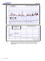
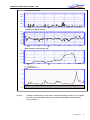
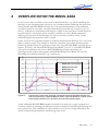
1
MOUSE RDII
USER GUIDE
MOUSE RDII
DHI Water & Environment
Agern Allé 11
DK-2970 Hørsholm
Denmark
Tel:
+45 4516 9200
Fax:
+45 4516 9292
E-mail: [email protected]
Web:
DHI Software
www.dhi.dk and www.dhisoftware.com
Contents
PART I - INTRODUCTION TO MOUSE RDII.....................................................................................1
1
ABOUT MOUSE RDII MODULE ...................................................................................................3
1.1 KEY FEATURES AND APPLICATION DOMAIN ......................................................................................3
1.2 SOFTWARE IMPLEMENTATION ..........................................................................................................3
2
ABOUT MOUSE RDII USER MANUAL .......................................................................................5
3
MOUSE RDII USER SUPPORT......................................................................................................7
3.1 PRODUCT SUPPORT...........................................................................................................................7
3.2 DHI TRAINING COURSES ..................................................................................................................7
3.3 COMMENTS AND SUGGESTIONS ........................................................................................................7
PART II - MOUSE RDII USER MANUAL .............................................................................................9
1
BACKGROUND ..............................................................................................................................11
2
DATA INPUT...................................................................................................................................12
2.1 OVERVIEW OF THE INPUT DATA FILES ..........................................................................................12
2.2 CATCHMENT DATA AND HYDROLOGICAL PARAMETERS ................................................................12
2.2.1 General .................................................................................................................................12
2.2.2 Definition of the RDI data.....................................................................................................12
2.2.3 Boundary Data Time Series ..................................................................................................12
3
EXECUTION OF THE MOUSE RDII COMPUTATIONS ........................................................12
3.1 THE RUNOFF COMPUTATION DIALOG ............................................................................................12
3.2 CHOICE OF CALCULATION TIME STEP............................................................................................12
3.3 THE RDII HOTSTART .....................................................................................................................12
4
THE RDII RESULT FILES............................................................................................................12
5
GENERAL DISCUSSION ..............................................................................................................12
6
SURFACE RUNOFF MODEL .......................................................................................................12
7
GENERAL HYDROLOGICAL MODEL - RDII .........................................................................12
8
OVERFLOW WITHIN THE MODEL AREA..............................................................................12
9
NON-PRECIPITATION DEPENDENT FLOW COMPONENTS .............................................12
REFERENCES .........................................................................................................................................12
MOUSE RDII
ii
DHI Software
Copyright
This document refers to proprietary computer software, which is protected by copyright.
All rights are reserved. Copying or other reproduction of this manual or the related
programs is prohibited without prior written consent of DHI Water & Environment1.
Warranty
The warranty given by DHI is limited as specified in your Software License Agreement.
The following should be noted: Because programs are inherently complex and may not be
completely free of errors, you are advised to validate your work. When using the programs,
you acknowledge that DHI has taken every care in the design of them. DHI shall not be
responsible for any damages arising out of the use and application of the programs and you
shall satisfy yourself that the programs provide satisfactory solutions by testing out
sufficient examples.
1 DHI is a private, non-profit research and consulting organization providing a broad spectrum of services and technology in
offshore, coastal, port, river, water resources, urban drainage and environmental engineering.
MOUSE RDII
iv
DHI Software
PART I - INTRODUCTION TO MOUSE RDII
DHI Software
1
MOUSE RDII
2
DHI Software
1
ABOUT MOUSE RDII MODULE
1.1
Key features and application domain
The MOUSE Rainfall Dependent Infiltration Module (RDII) provides detailed, continuous
modelling of the complete land phase of the hydrologic cycle, providing support for urban,
rural, and mixed catchments analyses. Precipitation is routed through four different types
of storage: snow, surface, unsaturated zone ("root-zone") and ground water. This enables
continuous modelling of the runoff processes, which is particularly useful when long-term
hydraulic and pollution load effects are analysed.
Instead of performing hydrological load analysis of the sewer system only for short periods
of high intensity rainstorms, a continuous, long-term analysis is applied to look at periods
of both wet and dry weather, as well as inflows and infiltration to the sewer network. This
provides a more accurate picture of actual loads on treatment plants and combined sewer
overflows. Further enhancements of groundwater-sewer interactions are possible by
implicit linking of the MOUSE Pipe model with DHI’s distributed groundwater model
MIKE SHE.
MOUSE RDII is particularly useful when used with MOUSE LTS, a specially developed
modelling tool for long-term network simulations and result statistics.
1.2
Software Implementation
MOUSE RDII is an add-on module to MOUSE HD Pipe Flow Model. The MOUSE
RDII capabilities can be accessed, i.e. continuous hydrology simulations can be executed,
only after the MOUSE license has been extended to include MOUSE RDII. MOUSE
RDII utilizes the standard MOUSE Menu System with on-line HELP facility, which has
been extended to accommodate some specific actions related to MOUSE RDII. This
implies that the MOUSE on-line HELP system and documentation related to the standard
versions of MOUSE are essential as a support for work with this module (ref./1/).
DHI Software
3
DHI Software
4
2
ABOUT MOUSE RDII USER MANUAL
This manual provides information related to the principles and techniques for the
preparation and execution of continuous hydrological simulations in urban, rural and
mixed catchments. It is assumed throughout this manual that the user is well acquainted
with the standard MOUSE system. Fundamental knowledge of hydrology also facilitates
the successful use of MOUSE RDII.
The User Manual contains a detailed information for usage of the MOUSE RDII, specific
instructions for input of the required data and calculation. Additionally, this general part is
supported with description of the calibration process – which is probably of essential
interest of all users.
The information concerning fundamental principles and methods which form the frame of
the MOUSE RDII concept is accessible in the associated MOUSE RDII - Reference
Manual.
Usage of the standard MOUSE and its’ other add-on modules is described in respective
user manuals & tutorials.
This manual is divided in three units:
!
Part I: Introduction
Some general information about MOUSE RDII and about this document.
!
Part II: MOUSE RDII User Manual
Basic information about MOUSE RDII simulation principles and techniques.
!
Part III: MOUSE RDII calibration tutorial
Comprehensive calibration guide.
DHI Software
5
MOUSE RDII
6
DHI Software
3
MOUSE RDII USER SUPPORT
3.1
Product Support
If you have questions or problems concerning MOUSE RDII, please consult the
documentation (MOUSE RDII User Guide as well as the RDII Reference Manual) first.
Secondly, look in the Releasenote. If you have access to the Internet, you may also have a
look at the MOUSE Home Page. The MOUSE Home Page is located at
http://www.dhisoftware.com/mouse.
If you cannot find the answer to your queries, please contact your local agent.
In countries where no local agent is present you may contact DHI directly, by mail, phone,
fax or e-mail:
DHI, Agern Allé 11, DK-2970 Hørsholm, Denmark
Phone: +45 45 169 200
Telefax: +45 45 169 292
e-mail: [email protected]
When you contact your local agent or DHI, you should prepare the following information:
"
"
"
"
"
3.2
The version number of MOUSE that you are using
The type of hardware you are using including available memory.
The exact wording of any messages that appeared on the screen.
A description of what happened and what you were doing when the problem
occurred.
A description of how you tried to solve the problem.
DHI Training Courses
DHI software is often used to solve complex and complicated problems, which requires a
good perception of modelling techniques and the capabilities of the software.
Therefore DHI provides training courses in the use of our products. A list of standard
courses is offered to our clients, ranging from introduction courses to courses for more
advanced users. The courses are advertised via DHI Software News and via DHI home
page on the Internet (http://www.dhi.dk).
DHI can adapt training courses to very specific subjects and personal wishes. DHI can also
assist you in your effort to build models applying the MOUSE software.
If you have any questions regarding DHI training courses do not hesitate to contact us.
3.3
Comments and Suggestions
Success in perception of the information presented in this document, together with the
user's general knowledge of urban sewer systems and experience in numerical modelling is
DHI Software
7
MOUSE RDII
essential for getting a maximum benefit from MOUSE RDII. This implies that the quality
of the documentation, in terms of presentation style, completeness and scientific and
engineering competence, constitutes an important aspect of the software product quality.
DHI will, therefore, appreciate any suggestion in that respect, hoping that future edition
will contribute to the improved overall quality of MOUSE RDII.
Please give your contribution via e-mail, fax or a letter.
8
DHI Software
PART II - MOUSE RDII USER MANUAL
DHI Software
9
MOUSE RDII
10
DHI Software
1
BACKGROUND
When studying the real flow conditions in sewer systems, flow peaks during rain events are
often found to exceed the values that can be attributed to the contribution from
participating impervious areas. This is a consequence of the phenomenon, usually named
Rainfall Induced Infiltration. This differs from the Rainfall Induced Inflow by the fact that
it does not depend only on the actual precipitation, but is heavily affected by the actual
hydrological situation, i.e. the "memory" from earlier hydrological events. For a certain
rainfall event, the increase in flow will therefore differ, depending on hydrological events
during the previous period. The Rainfall Induced Infiltration is also distinguished by a slow
flow response, which takes place during several days after the rainfall event.
From a hydrological point of view, parts of the infiltration behave in the same way as the
inflow. Therefore, classification of total hydrological loads to infiltration and inflow is not
suitable for modeling approach. Rather, to describe appropriately the constitutive
components of flow hydrographs, distinguished by their hydrological behavior, the
following concept is used instead:
!
FRC - Fast Response Component: comprises the rain induced inflow and fast
infiltration component;
!
SRC - Slow Response Component: comprises slow infiltration component.
Distinctive for the FRC component is that it is not influenced by the previous hydrological
situation, i.e. high or low soil moisture content. It occurs as a direct consequence of a
rainfall. The FRC component consists of the inflow to the sewer system and the fast flow
component of the infiltration, not dependent on previous hydrological conditions.
On the other hand, characteristic of the SRC component is that it is highly dependent on
the previous hydrological conditions and usually responses slowly to a rainfall. The SRC
component consists of the rest of the precipitation-induced infiltration and dry weather
infiltration/inflow.
When performing a numerical simulation of flows in sewer systems based on a traditional
approach, it is difficult to describe the effects of the SRC component. These effects can,
however, be of a great importance, especially when analyzing volumes, e.g. simulation of
the total inflow to the wastewater treatment plant and overflow volumes.
Figure 1 shows an example illustrating the influence of previous hydrological conditions
for the two components and their response to a rainfall.
DHI Software
11
MOUSE RDII
0
1
4.00
15
Flow (m3/s)
3.00
30
45
60
Rain-1 = Rain-2
FRC-1 ~ FRC-2
SRC-1 =/ SRC-2
2.00
75
90
Rainfall intensity (my-m/s)
LOW SOIL MOISTURE CONTENT
- DRY SEASON
Rain-1
FRC-1
1.00
105
120
SRC-1
FOULFLOW
0.00
01-01-99 00:00
01-01-99 12:00
02-01-99 00:00
135
02-01-99 12:00
03-01-99 00:00
0
1
4.00
15
Flow (m3/s)
3.00
45
60
2.00
75
FRC-2
90
1.00
105
120
SRC-2
FOULFLOW
0.00
01-01-99 00:00
Figure 1
30
Rainfall intensity (my-m/s)
HIGH SOIL MOISTURE CONTENT
- WET SEASON
Rain-2
01-01-99 12:00
02-01-99 00:00
135
02-01-99 12:00
03-01-99 00:00
Different catchment response under the same rainfall, due to different soil moisture
conditions at the beginning of the rainfall.
To accomplish a description of the discharge generated in sewer systems influenced by the
SRC component, a computation tool that considers the effects of previous hydrological
events is required. For that purpose, a general hydrological model MOUSE RDII has been
developed. MOUSE RDII permits generation of continuous hydrographs, thus allowing
for accurate simulations of single events as well as simulation of very long hydrological
periods.
MOUSE RDII is actually a combination of the MOUSE Surface Runoff model for the
description of the FRC component, and NAM - the hydrological model for the description
of the SRC component. 'NAM' is an abreviation of the Danish expression "Nedbør Afstrømnings-Model" . This model has been developed by the Hydrological Section of the
Institute of Hydrodynamics and Hydraulic Engineering at the Technical University of
Denmark.
12
DHI Software
BACKGROUND
A computational hydrological model such as the continuous part of RDII is a set of linked
mathematical statements describing, in a simplified quantitative form, the behavior of the
land phase of the hydrological cycle. The RDII model is a deterministic, conceptual,
lumped type of model with moderate input data requirements (see Figure 2).
Spatial characterization of constitutive parts of the analyzed area is achieved through
definition of sub-catchments - each of them described with a unique set of parameters.
This means that the model treats every sub-catchment as one unit. The parameters and
variables therefore represent an average for the whole sub-catchment.
MOUSE RDII calculates the total discharge (runoff and infiltration) within the catchment
area. This means that the hydraulic processes in the sewer system which affect the mass
balance (e.g. overflow) are not described and, therefore, this effect is not accounted for
when the total discharge from the catchment is calculated.
Precipitation
Evapo-transpiration
Routing
Snow Storage
Model A (Time-Area)
Model B (Kinematic Wave)
Model C (Linear Reservoir)
Fast Response
Surface Storage
Storage
Surface
Overland Flow
Slow Response
Root suction
Infiltration
InterFlow
Unsaturated Zone
Storage
Capilary flux
Ground Water
Recharge
Routing
Ground Water
Storage
Slow Response
Base Flow
Figure 2
Schematics of the RDII Model.
DHI Software
13
MOUSE RDII
14
DHI Software
2
DATA INPUT
2.1
Overview Of The Input Data Files
For the calculation with MOUSE RDII, the input data are organized in the following files:
2.2
!
*.HGF file (Catchments and Hydrological data file), containing the catchment
information, parameters for the selected surface runoff model, RDI parameters and
initial conditions data;
!
*.UND file, containing time series connections of meteorological data: rainfall,
temperature and potential evapo-transpiration.
Catchment Data and Hydrological Parameters
2.2.1 General
The process of data specification for catchments with SRC flow component, i.e. those
where MOUSE RDII computation should be activated, is practically equivalent to a
‘standard’ runoff model definition. The only additional effort is the activation of the RDI
(Rain Dependent Infiltration) component and definition of appropriate RDI model
parameters for the current catchment.
This implies that RDI is actually an extension of the MOUSE surface runoff models A and
B, adding the continuous SRC flow component to the discontinuous surface runoff
hydrographs (SRC). The total flow from a catchment is thus obtained just as a sum of the
two components.
The RDII data definition process consists so of the following steps:
!
Catchment definition, with fundamental catchment data. This process is identical as
for surface runoff models, as described in MOUSE User Guide.
!
Selection of the surface runoff model and definition of surface runoff model
parameters. This process is identical as for surface runoff models, as described in
MOUSE User Guide.
!
Activation of the RDI component and definition of the RDI parameters.
DHI Software
15
MOUSE RDII
Figure 3
The Catchments data dialog, with RDI section in the lower part.
2.2.2 Definition of the RDI data
The RDII computation for a certain catchment is activated by checking the RDI checkbox
on the “Catchments | Catchments” dialog. The essential additional information is the
extension of the RDI area (as percent of the total catchment area) and the selection of the
RDI parameter set.
If the RDI area is specified as 0%, the resulting RDI flow will be equal to zero, i.e. the
simulated flow will be equivalent to the surface runoff alone. If the field were left empty,
the system would issue a warning/error.
A RDI parameter set contains all RDI model parameters and initial conditions. MOUSE
comes with the ‘Default’ set, which can be edited to fit the specific needs. Furthermore, an
unlimited number of RDI parameter sets can be specified and associated with individual
catchments within the model setup, so that differences in hydrological characteristics,
catchment response time, initial water contents, etc. can be accounted for. RDI parameter
sets can be edited under the Menu option “Catchments | RDI Data”.
16
DHI Software
DATA INPUT
Figure 4
RDI Parameter Set dialog.
A detailed description and significance of various RDI parameters is provided in MOUSE
RDII – Technical Reference.
#
Evapo-transpiration and snowmelt are also applied in the surface runoff
computations. Since the control of these processes is possible only through the
RDI parameter sets, this means that they can only be activated if MOUSE RDII is
installed!
2.2.3 Boundary Data Time Series
Time series of boundary data for MOUSE RDII are stored to and manipulated by the
same database system as any other time series data in MOUSE. This implies that all
standard MOUSE facilities for the data input and presentation are at the user's disposal.
The required time series for an RDII simulation are precipitation (µm/s), temperature
(Deg. C) and potential evapo-transpiration (mm/hour).
As to avoid significant errors, it is important to consider the way in which the model
interprets the data stored in the time series database, i.e. how the values for intermediate
times are determined. For rain intensities and potential evapo-transpiration, the model
assumes a constant value since the last entered value. For other types of data, the model
interpolates linearly between the two neighboring values.
DHI Software
17
MOUSE RDII
18
DHI Software
3
3.1
EXECUTION OF THE MOUSE RDII
COMPUTATIONS
The Runoff Computation Dialog
The RDII computation is specified and started from the Runoff computation dialog
(“Catchments | Runoff Computation”). The RDII computation definition is very similar
to an ordinary surface runoff computation. The only differences are related to the
specification of HOTSTART conditions and the SRC simulation time step. Optionally, a
result file with detailed RDII results (*.NOF) can be specified.
Figure 5
3.2
The Computation Dialog.
Choice Of Calculation Time Step
When calculating with MOUSE RDII, time steps are given separately for the Surface
Runoff Model and for the rain dependent infiltration part.
The RDII calculation can often be performed with a relatively long time step (several
hours), while calculation with the Surface Runoff Model is typically performed with a time
step in order of value of several minutes.
The time step for Surface Runoff computations is defined following the general
considerations as described in MOUSE User Guide. This is primarily concerned about the
sufficient resolution of the runoff process in time.
Generally, the RDI simulation time step should be chosen in accordance with the
resolution of precipitation data, e.g. a time step of 24 hours could be suitable if only daily
precipitation data is available. However, in case when precipitation data with high
resolution of e.g. few minutes are available, the RDI time step should be chosen in
DHI Software
19
MOUSE RDII
accordance with the response of the discharge when raining. E.g., an RDI time step of 2 4 hours should be chosen, if the time constant CKOF is given a value of 8 hours.
To minimize the calculation time as well as the size of the result files the RDII calculations
are performed according to the following principle:
The RDII simulation is carried out continuously for the whole period specified. On the
contrary, the Surface Runoff simulation is carried-out only when raining. Thus, the start
time for the Surface Runoff calculation is set as the start time for rain hydrograph. The
Surface Runoff calculation continues until all the surface runoff hydrographs are regressed.
3.3
The RDII Hotstart
There is a HOTSTART facility included in MOUSE RDII, i.e. the initial conditions for the
various storages can be automatically taken from a former result file, at a simulation start
time.
The structure and contents of the result file used as a HOTSTART file requires that the
time series in the boundary connection start at least for the maximum specified
concentration time Tc earlier than the start time for the HOTSTART is specified. This is
required for the correct reconstruction of the surface runoff component (FRC).
20
DHI Software
4
THE RDII RESULT FILES
Two result files are generated by a MOUSE RDII calculation. These are:
!
*.CRF file, containing maximally five time series for each sub-catchment, namely:
- discharge, calculated with the Surface Runoff Model (the FRC component),
- discharge, calculated with the RDII model (the SRC component),
- total discharge,
- variation of water content in the surface storage for the Surface Runoff Model,
- variation of water content in the snow storage for the Surface Runoff Model.
The *.CRF file is used as input data for a MOUSE Pipe calculation.
!
*.NOF file (optional), containing detailed information about the processes treated
by a RDII- model, e.g.:
- different flow components in the RDI model,
- variation of water content in the different storage in the RDI model.
The *.NOF file is used for calibration of the SRC component.
In the *.CRF file the time series are saved with two various intervals, the shorter one for the
periods when the Surface Runoff Model is used, and a larger one in the remaining periods. In the
two other result files the time series are saved with the larger time interval, which is equal to the
time step used for the RDII calculation.
The RDII result files can be presented in MIKE View, as any other MOUSE result files.
DHI Software
21
MOUSE RDII
22
DHI Software
PART III - MOUSE RDII VALIDATION
DHI Software
23
MOUSE RDII
24
DHI Software
5
GENERAL DISCUSSION
Some of the parameters in MOUSE RDII (here meaning both for the rain dependent
inflow and the infiltration part) are related to actual physical data. However, the final
choice of parameter values must be based upon a comparison with historical measured
discharges, since a number of the parameters have an empirical character.
The available period of the measured discharge data and its resolution in time are of major
importance for the credibility of the obtained parameter values. Ideally, for a good
accuracy, a 3-5 years long time series of measured discharge data with daily values is
required for the calibration of the RDII parameters, see ref./4/. Several months long time
series with higher resolution, i.e. minutes or hours, depending on the size of the area, are
needed for the calibration of the surface runoff model. Measured time series with shorter
duration are also useful, although not securing optimal parameter values, see ref./4/. In
such case it is important that the time series represents different hydrological situations, i.e.
typical wet period or dry period.
An exact correspondence between simulations and measurements can however not be
expected and for areas where precipitation data of worse quality is used a less accurate
calibration result must be accepted. In this case it may be preferable to recall the purpose
of the actual model application and concentrate on calibrating yearly volumes, flow peaks
or base flows, depending on what kind of analysis is to be performed with the model.
It must be remembered that MOUSE RDII calculates the precipitation-dependent flow
component. When comparing with measured discharge data the total measured discharge
therefore has to be reduced with the flow components not being precipitation dependent,
e.g. foul flow, see Chapter 5 below.
MOUSE RDII calculates the total generated discharge from a catchment, i.e. overflow
within the sub-catchment will also be included in the calculated discharge. Therefore, when
comparing with measured peak flows and controlling the water balance (total volume) this
has to be taken into consideration (see Chapter 8).
In principle, the model validation is concerned about comparison of the computed and
measured hydrographs. As there are almost an infinite number of possibilities to describe
level of agreement between two hydrographs, it is recommended to establish some
validation criteria, i.e. a measure for accuracy of the model, relevant for current application.
There are several types of criteria, such as numeric criteria based on single values (e.g. peak
discharge, volume, etc), or more complex numeric criteria based on statistical analysis of
the computed and calculated time series. Also, there are different types of "visual" criteria,
based on visual inspection, e.g. comparison of graphic presentations of the calculated and
measured duration curves. An important issue is to find the most appropriate criteria for
the intended application of the model, see ref./5/.
The choice of criteria is important since it may affect the final choice of parameter values
and by that the behavior of the calibrated model. Numerical criteria are, however, limited
and therefore a visual comparison between the hydrographs is indispensable.
MOUSE supports visual comparison of the calculated time series with any time series of
the same type contained in the time series database. E.g., when validating the model, the
DHI Software
25
MOUSE RDII
calculated discharge can be plotted on the same graph with the measured discharge and
compared.
In the present version of MOUSE RDII there is no automatic calculation or evaluation of
specific numeric validation criteria as mentioned above. If appropriate, analysis of that type
can be conducted so that the calculated time series are exported to a spreadsheet or some
other program for further processing and comparison with measured time series.
Figures 6 and 7 show an example of calibration results for the catchment of Rya treatment
plant in Göteborg, Sweden, modeled as a MOUSE RDII area. Calibration was performed
for the years 1986 - 1989, and verification against independent data (not affecting the
choice of parameter values) for the years 1979 - 1984. Evaluation of the model validity in
this example was done through visual comparison of the hydrographs, study of the
accumulated difference and comparison between calculated and measured duration curve.
The obtained parameter values for this example are listed in Appendix I.
In the example related to the illustrations, overflow occurs within the model area. MOUSE
RDII can not describe this kind of processes (see Chapter 8), which complicates the choice
of validation criteria, see ref./5/.
26
DHI Software
GENERAL DISCUSSION
Calculated flow
Measured Flow
PART OF THE CALIBRATION PERIOD 1986-89
25.00
20.00
15.00
10.00
5.00
0.00
700
Accumulated flow
difference
600
500
400
300
Jan
1988
Feb
Mar
Apr
May
Duration curves for:
Calculated flow
Measured flow
m3/s
25.0
Jun
Jul
Aug
Sep
Oct
Nov
Dec
CALIBRATION PERIOD 1986 - 89
20.0
15.0
CSO Volume
10.0
5.0
0.0
0.0
Figure 6
0.2
0.4
0.6
0.8
1.0
Relative duration
Calibration results for the catchment of Rya, Göteborg, Sweden. Evaluation through
visual comparison of the hydrographs together with studies of the accumulated
difference between the hydrographs and comparison between calculated and
measured duration curve
DHI Software
27
MOUSE RDII
Calculated Flow
Measured Flow
m3/s
Part of the validation period 1979-84
25.0
20.0
15.0
10.0
5.0
0.0
400.0
Accumulated
difference in flow
300.0
200.0
100.0
0.0
Jan
1982
Feb
Mar
Apr
May
Jun
Duration curves for:
Jul
Aug
Sep
Oct
Nov
Dec
Validation period 1979-84
m3/s
Calculated Flow
Measured Flow
25.0
20.0
15.0
CSO volume
10.0
5.0
0.0
0.0
0.2
0.4
0.6
0.8
1.0
Relative duration
Figure 7
28
DHI Software
Calibration results for the catchment of Rya, Göteborg, Sweden. Evaluation through
visual comparison of the hydrographs, studies of the accumulated difference
between the hydrographs and comparison between calculated and measured
duration curve.
6
SURFACE RUNOFF MODEL
When simulating storm sewer systems or fully combined systems, usually a good estimation
of the area drained-off by the FRC component (impervious areas etc.) can be obtained
from physical data (maps etc.). The final model verification of a FRC should however be
based upon comparison with measured discharges during rainfall.
To separate the Afrc component (Surface Runoff Model) and the fast part of the SRC
component (Surface Runoff Component in RDII), measured discharge data with fairly
high resolution in time (hours) is required.
For calibration of the parameters describing the response of the discharge (e.g. tc and
TAtype for model A, or M, L and S for model B), a very high resolution in time is usually
required, minutes to hours.
DHI Software
29
MOUSE RDII
30
DHI Software
7
GENERAL HYDROLOGICAL MODEL - RDII
It is not possible to determine the RDII parameters from geophysical measurements, since
most of the parameters are of empirical nature. It is therefore necessary that measured
discharge from the studied area is available, so that the RDII parameters can be determined
by comparison between simulated and measured discharge through the calibration
procedure.
The introductory calibration is performed visually by comparing simulated and measured
discharge. The final optimization of the parameters is thereafter performed preferably
using different numeric and graphical criteria, see above and ref./6/.
The effects of changing each particular parameter are discussed below. Also, the most
suitable hydrological periods for calibrating certain parameters are identified, which implies
that a certain parameter affects the model behavior more during periods with specific
hydrological conditions. Usually, effects will also be obtained during other periods, why
these should also be studied when adjusting a parameter.
The parameters are discussed in the preferable order of adjustment. However, it may be
necessary to return to the previous calibration step, as well as repeating the whole process
several times. It is recommended, especially for less experienced users, that only one
parameter is changed at a time (i.e. for each calculation), so that the effect of the
adjustment will appear clearly.
Sometimes, however, the effect of changing one parameter is not sufficient. Then, several
parameters controlling similar phenomena can be adjusted together.
In some other cases, undesired secondary effects can be obtained when adjusting certain
model parameter. These effects can often be eliminated by simultaneously adjusting other
parameters, which do not influence the desired effects, but reduce secondary effects
induced by the first parameter.
The following sequence of action is recommended:
1.
The first step in the RDII calibration is usually to adjust the water balance in the
system, i.e. the accuracy between the calculated and measured total volume during
the observed period. This is done by correcting the proportion of area, Asrc. An
increase of Asrc proportionally increases every flow component at each time step.
The total volume generally also contains the runoff from impervious areas
(Surface Runoff Model) - see Chapter 6 and comments about overflow under
Chapter 8.
2.
Next, the overland flow coefficient CQOF is adjusted to obtain a correct
distribution of volume between overland flow (peak flows) and baseflow. This is
done after wet periods and preferably for a period with low evaporation.
A reduction of CQOF reduces the overland flow and increases the infiltration, i.e.
induces increase in the baseflow.
DHI Software
31
MOUSE RDII
The measured flow peaks generally also contain the runoff from impervious areas
(Surface Runoff Model), see Chapter 6 and comments about overflow under
Chapter 8.
3.
CKBF is adjusted against the response of the baseflow, i.e. the build-up and
regression of the baseflow. Adjustment against the built-up of baseflow is done
during and after wet periods with low evaporation. Adjustment against regression
is done during the start of dry periods with high evaporation, preferably when
baseflow is the only flow component.
An adjustment of CKBF does not influence the size of the discharged volume
studied for a longer period, but displaces the volumes in time.
4.
CKOF is adjusted against the response, i.e. the shape of the peak flows. This is
done during periods with heavy rainfall, preferably after a wet period.
The measured flow peaks generally also contain the runoff from impervious areas
(Surface Runoff Model), see Chapter 6 and comments about overflow under
Chapter 8.
5.
A reduction of Umax reduces the actual evapo-transpiration, the process
responsible for reduced discharges during period with high potential evaporation.
The effect of reducing Umax will be largest for periods preceded by a wet period.
Additionally, an increased overland flow is obtained, as well as more water
transported to the groundwater storage resulting in an delayed effect of increased
baseflow, because of the long response time of baseflow.
An important behavior of the RDII model is that the surface storage must be
filled-up before overland flow and infiltration, respectively, occur. Therefore,
during dry periods with high potential evaporation, Umax can be estimated from
how much rainfall is required for filling-up the surface storage, i.e. generating
overland flow. The same methodology can also be used for the periods with low
potential evaporation, but only if the rain event is preceded by a long dry period.
6.
CKIF is adjusted against the response of interflow during periods with low
potential evaporation. A reduction of CKIF will result in a small increase in volume
during these periods.
7.
The relative water content in the unsaturated zone (i.e. root-zone), L/Lmax
controls several of the different water transports in the RDII model. Since the
storage capacity, Lmax, influences the velocity of the filling of L towards Lmax, Lmax
is adjusted during periods of heavy filling of the root zone storage. This usually
occurs during periods with low potential evaporation preferably in combination
with a wet period.
A reduction of Lmax increases the discharge, but it may decrease a little during
period with very high potential evaporation.
8.
32
DHI Software
The threshold values indicate at which relative water content in the root zone,
L/Lmax, overland flow, interflow and baseflow respectively will be generated.
Therefore, the threshold values can be estimated from the time of filling the root
zone storage when each flow component starts discharging.
GENERAL HYDROLOGICAL MODEL - RDII
The threshold values have no effect during periods when the root zone storage is
full, L = Lmax.
An increased threshold value reduces the discharge during dry periods and in the
beginning of wet periods, i.e. periods with low relative water content in the root
zone storage.
TG is adjusted during periods with heavy filling of the root zone storage,
preferably in combination with low potential evaporation and preceded by a dry
period. TG is therefore an important parameter for adjusting the increase of the
groundwater level in the beginning of wet periods.
TOF is adjusted after a dry period at events with heavy filling of the root zone
storage. For example adjustment can be done for events where even larger rainfall
volumes does not generate overland flow.
TIF is adjusted after a dry period when filling of the root zone storage, preferably
in combination with low potential evaporation. However, TIF is one of the less
important parameters.
9.
The degree-day-coefficient, Csnow can be estimated from analysis of the relation
between temperature, water content in the snow storage and measured discharge.
When temperature is below zero, the precipitation is stored in the snow storage.
When temperature is above zero the content in the snow storage is emptied into
the surface storage, where the velocity of emptying is controlled by Csnow. An
increase of Csnow increases the emptying procedure.
This process should be addressed now and then during the whole calibration
procedure. Otherwise, there is a risk that a snow-melting phenomenon is
attempted to be described through adjusting other parameters.
10.
The Carea coefficient establishes the ratio of groundwater catchment and surface
catchment (per deafult, the two surfaces are equal). By changing the ratio, the ratio
between the baseflow and other runoff components is correspondingly changed.
The default values of the remaining RDII parameters: Sy (specific yield of the groundwater
reservoir), GWLmin (minimum groundwater depth), GWLBF0 (maximum groundwater
depth causing baseflow) and GWLFL1 (groundwater depth for unit capillary flux) are
adjusted only in exceptional cases. Therefore, these parameters have been included into the
RDII parameter set dialog in a separate "box". The effects of changing the default values
should be well understood prior to adjustment.
Figure 8 shows an example of the build-up of the snow cover, followed by the snowmelting process. The calculated and measured flow reactions during the same period are
shown. The example is from the treatment plant at Duvbacken, Gävle, Sweden, see
ref./5/. Considering the complexity of the snow melting process within urban areas, a
fairly good description was obtained with the RDII model.
Since the variation of water contents in the surface and root zone storage controls many of
the other processes, they should be studied continuously throughout the calibration
procedure. Figure 9 shows an example of the variation of water content in the surface
storage, root zone storage and groundwater storage. The example comes from the
DHI Software
33
MOUSE RDII
catchment of Rya treatment plant, Göteborg, Sweden. It appears that the root zone storage
is emptied only during the summer period, because the evaporation during the rest of the
year is almost non-existent. Discharge from the groundwater storage exists continuously all
year around. Drawing of the surface storage is faster during summer period since the
evaporation is high, and is therefore the dominating effect on the surface storage. During
periods with low evaporation, drawing of the surface storage is controlled by the given
time constant for interflow, CKIF.
The example also shows that filling of the root zone and groundwater storage only occurs
when the surface storage is completely filled, i.e. when precipitation has filled-up the
surface storage. A larger surface storage, i.e. a larger Umax, will therefore imply that this
happens more rarely and at a smaller extent, allowing a larger part of the precipitation to
evaporate.
A smaller root zone storage, i.e. a smaller Lmax, would have led to an increased relative
variation in the storage. Furthermore, the actual evaporation will decrease in case of smaller
root zone storage, because less water is available for the vegetation to draw water for
transpiration, mainly during summer period.
Monthly and yearly values for the different processes, e.g. precipitation volume, real
evaporation and total discharge, are written to an ASCII file, NAMSTAT.TXT after every
RDII calculation. It is recommended that the content of this file is studied now and then
during the calibration procedure.
34
DHI Software
GENERAL HYDROLOGICAL MODEL - RDII
Precipitation, mm/hour
2.500
2.000
1.500
1.000
0.500
0.000
Nov
1987
Jan
1988
Dec
Feb
Mar
Apr
Temperature, degrees Celsius
20.0
15.0
10.0
5.0
0.0
-5.0
-10.0
-15.0
-20.0
Nov
1987
Dec
Jan
1988
Feb
Mar
Feb
Mar
Apr
Water content in snow storage, mm
200.0
150.0
100.0
50.0
0.0
Nov
1987
Dec
Jan
1988
Apr
Measured Flow
Calculated Flow, m3/s
2.0
1.5
1.0
0.5
Foul Flow
0.0
Figure 8
Nov
1987
Dec
Jan
1988
Feb
Mar
Apr
Example of the build-up of snow cover, followed by melting process and calculated
and measured discharge during the same period, Duvbackens treatment plant,
Gävle, Sweden
DHI Software
35
MOUSE RDII
Relative water conte nt, root zone s torage, L
Relative water conte nt, surfa ce storage, U
1.0
0.8
0.6
0.4
0.2
0.0
Jan
1988
Feb
Mar
Apr
May
Jun
Jul
Aug
Sep
Aug
Sep
Oct
Nov
Dec
Nov
Dec
Ground w ater depth, m eter
-8.0
-8.5
-9.0
-9.5
-10.0
Jan
Feb
Mar
Apr
May
Jun
Jul
Oct
1988
Figure 9
36
DHI Software
Example of the variation of water content in the surface storage, root zone storage
and the groundwater storage.
8
OVERFLOW WITHIN THE MODEL AREA
In those cases when overflow occurs in the studied model area, e.g. when simulating the
discharge to the treatment plant, this has to be considered when calibrating the peak flows
during rainfall. MOUSE RDII calculates the total generated discharge in the catchment
area and is therefore not able to describe hydraulic processes like e.g. overflow (“loss of
water”). Calibration of parameters affecting the volume in the peak flows should therefore
be performed for rain events, when overflow is unlikely to occur. Model parameters
affecting the response of the discharge, for rain events when overflow occur, can be
calibrated against the peak flows base or width.
Figure 10 shows the agreement between calculated and measured discharge for a rain event
when overflow occurs. The example is from the catchment area to Rya treatment plant,
Göteborg, Sweden. Both the agreements when only using MOUSE RDII (a model area of
approx. 212 km2), and when MOUSE Pipe Flow Model, (see ref./1/) and MOUSE RDII
are used in combination are shown. MOUSE RDII was used for describing the
hydrological load (inflow hydrographs) while MOUSE Pipe Flow Model was used for
describing the hydraulic processes, e.g. overflow etc.
m3/s
35.0
30.0
MOUSE RDII - Total discharge
MOUSE RDII - Excl. FRC
25.0
MOUSE RDII + HD
Measured Flow
20.0
15.0
10.0
5.0
0.0
19 / 7
20 / 7
21 / 7
21 / 7
1988
Figure 10
Comparison of measured discharge, discharge calculated with MOUSE RDII and
flow calculated with a combined MOUSE RDII / Pipe Flow Model for a heavy rainfall
event where overflow occurs upstream from the measurement point.
A well-calibrated MOUSE RDII model can therefore be used for a rough estimation of
overflow volume by studying the difference between calculated and measured discharge for
heavy peak flows. The credibility for such estimation is however strongly affected by the
quality of measured precipitation and discharge time series.
DHI Software
37
MOUSE RDII
38
DHI Software
9
NON-PRECIPITATION DEPENDENT FLOW
COMPONENTS
MOUSE RDII calculates the precipitation dependent flow component. Therefore, both for
calibration and validation, other flow components should be treated outside MOUSE
RDII.
Examples of non-precipitation dependent flow components are foul flow and sea-water
leaking into the sewer system.
The foul flow is preferably estimated through daily values from produced water volumes
weighted with yearly charged water volumes. This will however only give a rough
estimation, why departure from this methodology may be necessary, e.g. for areas where a
large amount of freshwater is used for irrigation.
The amount of leaking sea-water is preferably estimated through an iterative procedure
between MOUSE RDII calculation and studies of the difference between the calculated
and measured discharge. Only a rough estimation can be achieved, why less accurate
calibration results may have to be accepted.
Specially, during the calibration procedure it is very important that non-hydrological errors
generally are kept at the lowest level possible in the flow series used. Otherwise, there is a
risk of hydrological interpretations of these errors, the error transmitting in the model and
increasing when simulating extreme hydrological situations. A typical example is a rough
resolution in time for the foul flow component. The method described above should give a
description sufficiently correct for most cases.
DHI Software
39
MOUSE RDII
40
DHI Software
REFERENCES
/1/
DHI (2000): MOUSE - User Manual and Tutorial (Version 2000), DHI,
Hørsholm, Denmark.
/3/
DHI (1992): NAM - User Manual and Reference Manual, DHI, Hørsholm,
Denmark.
/4/
Eriksson, B., (1983): Data concerning the precipitation climate of Sweden.
Mean values for the period 1951-80. Rapport 1983:28, SMHI, Norrköping,
Sweden (in Swedish).
/5/
Gustafsson, A.M., (1992): The hydrological model NAM. The Calibration
periods' effect on model parameters and valuation results. Thesis project,
Department of hydraulics, Chalmers University of Technology, Göteborg, Sweden
(in Swedish).
/6/
Gustafsson, L.G., (1992): Modeling of urban hydrology. User's guide MouseNAM. VA-forsk rapport nr 1993-04, VAV, Stockhom, Sweden (in
Swedish).
/7/
Niemczynowicz, J., (1984): An investigation of the areal properties of rainfall
and its influence on runoff generating processes. Institutionen för teknisk
vattenresurslära, Lunds Tekniska Högskola, Lund, Sweden.
/8/
Wilson, E.M., (1990): Engineering Hydrology. 4th edition, Macmillan Education
Ltd, London.
DHI Software
41
MOUSE RDII
42
DHI Software
APPENDIX I :
Examples of MOUSE RDII Parameter Sets
Parameter sets obtained for a number of MOUSE RDII applications are presented in this
Appendix.
The parameters for the response function of the surface runoff modes - Time/Area
method (A) or Kinematic wave method (B), have not been given since the surface runoff
model was not used for simulating the FRC component (impervious areas etc.) for the
presented applications. The FRC component was instead simulated as a fictitious RDII
area, the parameters chosen so that only overland flow occurs. Therefore, the response for
the FRC component is described using the RDI parameter CKOF instead, and thus given
below.
For the RDI parameters not specified, MOUSE RDI default values were used.
EXAMPLE 1:
Catchment area - Rya treatment plant, Göteborg, Sweden
Aurb
212.0
Afrc
10.4
km2
%
Asrc
Surface runoff model
RDI-model
Umax
0.6
mm
Umax 5.0
Lmax 180.0
CKof
7.0
hours
Csnow
5.0
mm/C/day
CQof
51.7
%
mm
mm
0.35
CKof 18.0
CKif 150.0
CKbf 2000.0
hours
hours
hours
Tof 15.0 % of Lmax
Tif 0.0 % of Lmax
Tg
0.0 % of Lmax
Csnow
3.0
mm/C/day
DHI Software
43
MOUSE RDII
EXAMPLE 2:
Catchment area - Kalmar treatment plant, Sweden
Aurb
Afrc
33.0
km2
3.0
%
Asrc 23.0
Surface runoff model
RDI-model
Umax
0.6
mm
Umax 10.0
Lmax 150.0
CKof
1.5
hours
Csnow
2.5
mm/C/day
CQof
%
mm
mm
0.05
CKof 10.0
CKif 400.0
CKbf 800.0
hours
hours
hours
Tof 27.0 % of Lmax
Tif 63.0 % of Lmax
Tg 23.0 % of Lmax
Csnow
44
DHI Software
2.5
mm/C/day
APPENDIX I
EXAMPLE 3:
Catchment area - Halmstad treatment plant, Sweden
Aurb
Afrc
26.0 km2
7.7 %
Asrc 46.0
Surface runoff model
RDI-model
Umax
0.6
mm
Umax 5.0
Lmax 200.0
CKof
1.5
hours
Csnow
-
CQof
%
mm
mm
0.10
mm/C/day
CKof 30.0 hours
Ckif
500.0 hours
CKbf 2500.0 hours
Tof 40.0 % of Lmax
Tif 20.0 % of Lmax
Tg 20.0 % of Lmax
Csnow
-
mm/C/day
DHI Software
45
MOUSE RDII
EXAMPLE 4:
Catchment area - Trollhättan treatment plant, Sweden
Aurb
22.0
km2
Afrc
15.0
%
Asrc 77.0
Surface runoff model
RDI-model
Umax
0.6
mm
Umax 5.0
Lmax 200.0
CKof
6.0
hours
Csnow
3.0
mm/C/day
CQof
%
mm
mm
0.45
CKof 20.0
CKif 200.0
CKbf 1000.0
hours
hours
hours
Tof 40.0 % of Lmax
Tif 0.0 % of Lmax
Tg
0.0 % of Lmax
Csnow
46
DHI Software
3.0
mm/C/day
APPENDIX I
EXAMPLE 5:
Catchment area - Hedesunda treatment plant, Gävle, Sweden
Aurb
2.3
km2
Afrc
0.9
%
Asrc 16.1
Surface runoff model
RDI-model
Umax
0.6
mm
Umax 10.0
Lmax 100.0
CKof
1.0
hours
Csnow
7.0
mm/C/day
CQof
%
mm
mm
0.25
CKof 10.0
CKif 600.0
CKbf 1200.0
hours
hours
hours
Tof 0.0 % of Lmax
Tif 0.0 % of Lmax
Tg 0.0 % of Lmax
Csnow
7.0
mm/C/day
DHI Software
47
MOUSE RDII
EXAMPLE 6:
Catchment area - Styrsö treatment plant, Göteborg, Sweden
Aurb
1.4
km2
Afrc
0.8
%
Asrc 23.0
Surface runoff model
RDI-model
Umax
0.6
mm
Umax 13.0
Lmax 200.0
CKof
1.5
hours
Csnow
5.0
mm/C/day
CQof
%
mm
mm
0.70
CKof 20.0
CKif 600.0
CKbf 1500.0
hours
hours
hours
Tof 0.0 % of Lmax
Tif 0.0 % of Lmax
Tg 0.0 % of Lmax
Csnow
48
DHI Software
5.0
mm/C/day