1
CalculiX USER’S MANUAL
- CalculiX GraphiX, Version 2.5 Klaus Wittig
September 27, 2012
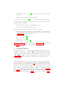
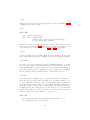
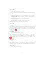
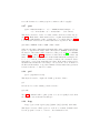
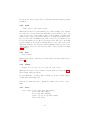
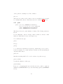
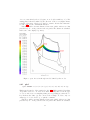
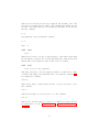
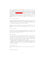
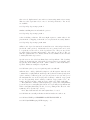
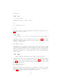
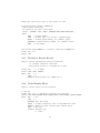
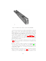
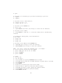
Figure 1: A complex model made from scratch using second order brick elements
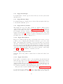
1
Contents
1 Introduction
6
2 Concept
7
3 File Formats
8
4 Getting Started
9
5 Program Parameters
13
6 Input Devices
14
6.1 Mouse . . . . . . . . . . . . . . . . . . . . . . . . . . . . . . . . . 14
6.2 Keyboard . . . . . . . . . . . . . . . . . . . . . . . . . . . . . . . 14
7 Menu
7.1 Datasets . . . . . . . . . . . . . . .
7.1.1 Entity . . . . . . . . . . . .
7.2 Viewing . . . . . . . . . . . . . . .
7.2.1 Show Elements With Light
7.2.2 Show Bad Elements . . . .
7.2.3 Fill . . . . . . . . . . . . . .
7.2.4 Lines . . . . . . . . . . . . .
7.2.5 Dots . . . . . . . . . . . . .
7.2.6 Toggle Culling Back/Front
7.2.7 Toggle Model Edges . . . .
7.2.8 Toggle Element Edges . . .
7.2.9 Toggle Surfaces/Volumes .
7.2.10 Toggle Move-Z/Zoom . . .
7.2.11 Toggle Background Color .
7.2.12 Toggle Vector-Plot . . . . .
7.2.13 Toggle Add-Displacement .
7.3 Animate . . . . . . . . . . . . . . .
7.3.1 Start . . . . . . . . . . . . .
7.3.2 Tune-Value . . . . . . . . .
7.3.3 Steps per Period . . . . . .
7.3.4 Time per Period . . . . . .
7.3.5 Toggle Real Displacements
7.3.6 Toggle Dataset Sequence . .
7.4 Frame . . . . . . . . . . . . . . . .
7.5 Zoom . . . . . . . . . . . . . . . .
7.6 Center . . . . . . . . . . . . . . . .
7.7 Enquire . . . . . . . . . . . . . . .
7.8 Cut . . . . . . . . . . . . . . . . .
7.9 Graph . . . . . . . . . . . . . . . .
7.10 Orientation . . . . . . . . . . . . .
2
.
.
.
.
.
.
.
.
.
.
.
.
.
.
.
.
.
.
.
.
.
.
.
.
.
.
.
.
.
.
.
.
.
.
.
.
.
.
.
.
.
.
.
.
.
.
.
.
.
.
.
.
.
.
.
.
.
.
.
.
.
.
.
.
.
.
.
.
.
.
.
.
.
.
.
.
.
.
.
.
.
.
.
.
.
.
.
.
.
.
.
.
.
.
.
.
.
.
.
.
.
.
.
.
.
.
.
.
.
.
.
.
.
.
.
.
.
.
.
.
.
.
.
.
.
.
.
.
.
.
.
.
.
.
.
.
.
.
.
.
.
.
.
.
.
.
.
.
.
.
.
.
.
.
.
.
.
.
.
.
.
.
.
.
.
.
.
.
.
.
.
.
.
.
.
.
.
.
.
.
.
.
.
.
.
.
.
.
.
.
.
.
.
.
.
.
.
.
.
.
.
.
.
.
.
.
.
.
.
.
.
.
.
.
.
.
.
.
.
.
.
.
.
.
.
.
.
.
.
.
.
.
.
.
.
.
.
.
.
.
.
.
.
.
.
.
.
.
.
.
.
.
.
.
.
.
.
.
.
.
.
.
.
.
.
.
.
.
.
.
.
.
.
.
.
.
.
.
.
.
.
.
.
.
.
.
.
.
.
.
.
.
.
.
.
.
.
.
.
.
.
.
.
.
.
.
.
.
.
.
.
.
.
.
.
.
.
.
.
.
.
.
.
.
.
.
.
.
.
.
.
.
.
.
.
.
.
.
.
.
.
.
.
.
.
.
.
.
.
.
.
.
.
.
.
.
.
.
.
.
.
.
.
.
.
.
.
.
.
.
.
.
.
.
.
.
.
.
.
.
.
.
.
.
.
.
.
.
.
.
.
.
.
.
.
.
.
.
.
.
.
.
.
.
.
.
.
.
.
.
.
.
.
.
.
.
.
.
.
.
.
.
.
.
.
.
.
.
.
.
.
.
.
.
.
.
.
.
.
.
.
.
.
.
.
.
.
.
.
.
.
.
.
.
.
.
.
.
.
.
.
.
.
.
.
.
.
.
.
.
.
.
.
.
.
.
.
.
.
.
.
.
.
.
.
.
.
.
.
.
.
.
.
.
.
.
.
.
.
.
.
.
.
.
.
.
.
.
.
.
15
15
16
17
17
17
17
17
17
17
18
18
18
18
18
18
19
19
19
19
19
19
19
20
20
20
20
20
20
21
21
7.10.1 +x View . . . . . . . . . . .
7.10.2 -x View . . . . . . . . . . .
7.10.3 +y View . . . . . . . . . . .
7.10.4 -y View . . . . . . . . . . .
7.10.5 +z View . . . . . . . . . . .
7.10.6 -z View . . . . . . . . . . .
7.11 Hardcopy . . . . . . . . . . . . . .
7.11.1 Tga-Hardcopy . . . . . . .
7.11.2 Ps-Hardcopy . . . . . . . .
7.11.3 Gif-Hardcopy . . . . . . . .
7.11.4 Png-Hardcopy . . . . . . .
7.11.5 Start Recording Gif-Movie .
7.12 Help . . . . . . . . . . . . . . . . .
7.13 Quit . . . . . . . . . . . . . . . . .
8 Commands
8.1 area . .
8.2 asgn . .
8.3 bia . . .
8.4 body . .
8.5 call . . .
8.6 cntr . .
8.7 comp . .
8.8 copy . .
8.9 corrad .
8.10 cut . . .
8.11 del . . .
8.12 div . . .
8.13 ds . . .
8.14 elem . .
8.15 elty . . .
8.16 enq . . .
8.17 eqal . .
8.18 exit . . .
8.19 flip . . .
8.20 flpc . . .
8.21 font . .
8.22 frame .
8.23 gbod . .
8.24 gonly . .
8.25 graph .
8.26 grps . .
8.27 gsur . .
8.28 gtol . .
8.29 hcpy . .
8.30 help . .
.
.
.
.
.
.
.
.
.
.
.
.
.
.
.
.
.
.
.
.
.
.
.
.
.
.
.
.
.
.
.
.
.
.
.
.
.
.
.
.
.
.
.
.
.
.
.
.
.
.
.
.
.
.
.
.
.
.
.
.
.
.
.
.
.
.
.
.
.
.
.
.
.
.
.
.
.
.
.
.
.
.
.
.
.
.
.
.
.
.
.
.
.
.
.
.
.
.
.
.
.
.
.
.
.
.
.
.
.
.
.
.
.
.
.
.
.
.
.
.
.
.
.
.
.
.
.
.
.
.
.
.
.
.
.
.
.
.
.
.
.
.
.
.
.
.
.
.
.
.
.
.
.
.
.
.
.
.
.
.
.
.
.
.
.
.
.
.
.
.
.
.
.
.
.
.
.
.
.
.
.
.
.
.
.
.
.
.
.
.
.
.
.
.
.
.
.
.
.
.
.
.
.
.
.
.
.
.
.
.
.
.
.
.
.
.
.
.
.
.
.
.
.
.
.
.
.
.
.
.
.
.
.
.
.
.
.
.
.
.
.
.
.
.
.
.
.
.
.
.
.
.
.
.
.
.
.
.
.
.
.
.
.
.
.
.
.
.
.
.
.
.
.
.
.
.
.
.
.
.
.
.
.
.
.
.
.
.
.
.
.
.
.
.
.
.
.
.
.
.
.
.
.
.
.
.
.
.
.
.
.
.
.
.
.
.
.
.
.
.
.
.
.
.
.
.
.
.
.
.
.
.
.
.
.
.
.
.
.
.
.
.
.
.
.
.
.
.
.
.
.
.
.
.
.
.
.
.
.
.
.
.
.
.
.
.
.
.
.
.
.
.
.
.
.
.
.
.
.
.
.
.
.
.
.
.
.
.
.
.
3
.
.
.
.
.
.
.
.
.
.
.
.
.
.
.
.
.
.
.
.
.
.
.
.
.
.
.
.
.
.
.
.
.
.
.
.
.
.
.
.
.
.
.
.
.
.
.
.
.
.
.
.
.
.
.
.
.
.
.
.
.
.
.
.
.
.
.
.
.
.
.
.
.
.
.
.
.
.
.
.
.
.
.
.
.
.
.
.
.
.
.
.
.
.
.
.
.
.
.
.
.
.
.
.
.
.
.
.
.
.
.
.
.
.
.
.
.
.
.
.
.
.
.
.
.
.
.
.
.
.
.
.
.
.
.
.
.
.
.
.
.
.
.
.
.
.
.
.
.
.
.
.
.
.
.
.
.
.
.
.
.
.
.
.
.
.
.
.
.
.
.
.
.
.
.
.
.
.
.
.
.
.
.
.
.
.
.
.
.
.
.
.
.
.
.
.
.
.
.
.
.
.
.
.
.
.
.
.
.
.
.
.
.
.
.
.
.
.
.
.
.
.
.
.
.
.
.
.
.
.
.
.
.
.
.
.
.
.
.
.
.
.
.
.
.
.
.
.
.
.
.
.
.
.
.
.
.
.
.
.
.
.
.
.
.
.
.
.
.
.
.
.
.
.
.
.
.
.
.
.
.
.
.
.
.
.
.
.
.
.
.
.
.
.
.
.
.
.
21
21
21
21
21
21
21
21
22
22
22
22
22
22
.
.
.
.
.
.
.
.
.
.
.
.
.
.
.
.
.
.
.
.
.
.
.
.
.
.
.
.
.
.
.
.
.
.
.
.
.
.
.
.
.
.
.
.
.
.
.
.
.
.
.
.
.
.
.
.
.
.
.
.
.
.
.
.
.
.
.
.
.
.
.
.
.
.
.
.
.
.
.
.
.
.
.
.
.
.
.
.
.
.
.
.
.
.
.
.
.
.
.
.
.
.
.
.
.
.
.
.
.
.
.
.
.
.
.
.
.
.
.
.
.
.
.
.
.
.
.
.
.
.
.
.
.
.
.
.
.
.
.
.
.
.
.
.
.
.
.
.
.
.
.
.
.
.
.
.
.
.
.
.
.
.
.
.
.
.
.
.
.
.
.
.
.
.
.
.
.
.
.
.
.
.
.
.
.
.
.
.
.
.
.
.
.
.
.
.
.
.
.
.
.
.
.
.
.
.
.
.
.
.
.
.
.
.
.
.
.
.
.
.
.
.
.
.
.
.
.
.
.
.
.
.
.
.
.
.
.
.
.
.
.
.
.
.
.
.
.
.
.
.
.
.
.
.
.
.
.
.
.
.
.
.
.
.
.
.
.
.
.
.
.
.
.
.
.
.
.
.
.
.
.
.
.
.
.
.
.
.
.
.
.
.
.
.
.
.
.
.
.
.
.
.
.
.
.
.
.
.
.
.
.
.
.
.
.
.
.
.
.
.
.
.
.
.
.
.
.
.
.
.
.
.
.
.
.
.
.
.
.
.
.
.
.
.
.
.
.
.
.
.
.
.
.
.
.
.
.
.
.
.
.
.
.
.
.
.
.
.
.
.
.
.
.
.
.
.
.
.
.
.
.
.
.
.
.
.
.
.
.
.
.
.
.
.
.
.
.
.
.
.
.
.
.
.
.
.
.
.
.
.
.
.
.
.
.
.
.
.
.
.
.
.
.
.
.
.
.
.
.
.
.
.
.
.
.
.
.
.
.
.
.
.
.
.
.
.
.
.
.
.
.
.
.
.
.
.
.
.
.
.
.
.
.
.
.
.
.
.
.
.
.
.
.
.
.
.
.
.
.
.
.
.
.
.
.
.
.
.
.
.
.
.
.
.
.
.
.
.
.
.
.
.
.
.
.
.
.
.
.
.
22
23
23
24
24
25
25
25
26
27
27
28
29
29
30
31
31
33
33
33
33
33
34
34
34
35
36
37
37
37
38
8.31
8.32
8.33
8.34
8.35
8.36
8.37
8.38
8.39
8.40
8.41
8.42
8.43
8.44
8.45
8.46
8.47
8.48
8.49
8.50
8.51
8.52
8.53
8.54
8.55
8.56
8.57
8.58
8.59
8.60
8.61
8.62
8.63
8.64
8.65
8.66
8.67
8.68
8.69
8.70
8.71
8.72
8.73
8.74
8.75
8.76
lcmb .
length
line . .
mata .
map .
mats .
max .
merg .
mesh .
mids .
min .
minus
move .
movi .
msg .
node .
nurl .
nurs .
ori . .
plot .
plus .
pnt . .
prnt .
proj .
qadd .
qali . .
qbia .
qbod .
qcnt .
qcut .
qdel .
qdis .
qdiv .
qele .
qenq .
qfil . .
qflp . .
qint .
qlin . .
qnor .
qpnt .
qnod .
qrem .
qseq .
qshp .
qspl .
.
.
.
.
.
.
.
.
.
.
.
.
.
.
.
.
.
.
.
.
.
.
.
.
.
.
.
.
.
.
.
.
.
.
.
.
.
.
.
.
.
.
.
.
.
.
.
.
.
.
.
.
.
.
.
.
.
.
.
.
.
.
.
.
.
.
.
.
.
.
.
.
.
.
.
.
.
.
.
.
.
.
.
.
.
.
.
.
.
.
.
.
.
.
.
.
.
.
.
.
.
.
.
.
.
.
.
.
.
.
.
.
.
.
.
.
.
.
.
.
.
.
.
.
.
.
.
.
.
.
.
.
.
.
.
.
.
.
.
.
.
.
.
.
.
.
.
.
.
.
.
.
.
.
.
.
.
.
.
.
.
.
.
.
.
.
.
.
.
.
.
.
.
.
.
.
.
.
.
.
.
.
.
.
.
.
.
.
.
.
.
.
.
.
.
.
.
.
.
.
.
.
.
.
.
.
.
.
.
.
.
.
.
.
.
.
.
.
.
.
.
.
.
.
.
.
.
.
.
.
.
.
.
.
.
.
.
.
.
.
.
.
.
.
.
.
.
.
.
.
.
.
.
.
.
.
.
.
.
.
.
.
.
.
.
.
.
.
.
.
.
.
.
.
.
.
.
.
.
.
.
.
.
.
.
.
.
.
.
.
.
.
.
.
.
.
.
.
.
.
.
.
.
.
.
.
.
.
.
.
.
.
.
.
.
.
.
.
.
.
.
.
.
.
.
.
.
.
.
.
.
.
.
.
.
.
.
.
.
.
.
.
.
.
.
.
.
.
.
.
.
.
.
.
.
.
.
.
.
.
.
.
.
.
.
.
.
.
.
.
.
.
.
.
.
.
.
.
.
.
.
.
.
.
.
.
.
.
.
.
.
.
.
.
.
.
.
.
.
.
.
.
.
.
.
.
.
.
.
.
.
.
.
.
.
.
.
.
.
.
.
.
.
.
.
.
.
.
.
.
.
.
.
.
.
.
.
.
.
.
.
.
.
.
.
.
.
.
.
.
.
.
.
.
.
.
.
.
.
.
.
.
.
.
.
.
.
.
.
.
.
.
.
.
.
.
.
.
.
.
.
.
.
.
.
.
.
.
.
.
.
.
.
.
.
.
.
.
.
.
.
.
.
.
.
.
.
.
.
.
.
.
.
.
.
.
.
.
.
.
.
.
.
.
.
.
.
.
.
.
.
.
.
.
.
.
.
.
.
.
.
.
.
.
.
.
.
.
.
.
.
.
.
.
.
.
.
.
.
.
.
.
.
.
.
.
.
.
.
.
.
.
.
.
.
.
.
.
.
.
.
.
.
.
.
.
.
.
.
.
.
.
.
.
.
.
.
.
.
.
.
.
.
.
.
.
.
.
.
.
.
.
.
.
.
.
.
.
.
.
.
.
.
.
.
.
.
.
.
.
.
.
.
.
.
.
.
.
.
.
.
.
.
.
4
.
.
.
.
.
.
.
.
.
.
.
.
.
.
.
.
.
.
.
.
.
.
.
.
.
.
.
.
.
.
.
.
.
.
.
.
.
.
.
.
.
.
.
.
.
.
.
.
.
.
.
.
.
.
.
.
.
.
.
.
.
.
.
.
.
.
.
.
.
.
.
.
.
.
.
.
.
.
.
.
.
.
.
.
.
.
.
.
.
.
.
.
.
.
.
.
.
.
.
.
.
.
.
.
.
.
.
.
.
.
.
.
.
.
.
.
.
.
.
.
.
.
.
.
.
.
.
.
.
.
.
.
.
.
.
.
.
.
.
.
.
.
.
.
.
.
.
.
.
.
.
.
.
.
.
.
.
.
.
.
.
.
.
.
.
.
.
.
.
.
.
.
.
.
.
.
.
.
.
.
.
.
.
.
.
.
.
.
.
.
.
.
.
.
.
.
.
.
.
.
.
.
.
.
.
.
.
.
.
.
.
.
.
.
.
.
.
.
.
.
.
.
.
.
.
.
.
.
.
.
.
.
.
.
.
.
.
.
.
.
.
.
.
.
.
.
.
.
.
.
.
.
.
.
.
.
.
.
.
.
.
.
.
.
.
.
.
.
.
.
.
.
.
.
.
.
.
.
.
.
.
.
.
.
.
.
.
.
.
.
.
.
.
.
.
.
.
.
.
.
.
.
.
.
.
.
.
.
.
.
.
.
.
.
.
.
.
.
.
.
.
.
.
.
.
.
.
.
.
.
.
.
.
.
.
.
.
.
.
.
.
.
.
.
.
.
.
.
.
.
.
.
.
.
.
.
.
.
.
.
.
.
.
.
.
.
.
.
.
.
.
.
.
.
.
.
.
.
.
.
.
.
.
.
.
.
.
.
.
.
.
.
.
.
.
.
.
.
.
.
.
.
.
.
.
.
.
.
.
.
.
.
.
.
.
.
.
.
.
.
.
.
.
.
.
.
.
.
.
.
.
.
.
.
.
.
.
.
.
.
.
.
.
.
.
.
.
.
.
.
.
.
.
.
.
.
.
.
.
.
.
.
.
.
.
.
.
.
.
.
.
.
.
.
.
.
.
.
.
.
.
.
.
.
.
.
.
.
.
.
.
.
.
.
.
.
.
.
.
.
.
.
.
.
.
.
.
.
.
.
.
.
.
.
.
.
.
.
.
.
.
.
.
.
.
.
.
.
.
.
.
.
.
.
.
.
.
.
.
.
.
.
.
.
.
.
.
.
.
.
.
.
.
.
.
.
.
.
.
.
.
.
.
.
.
.
.
.
.
.
.
.
.
.
.
.
.
.
.
.
.
.
.
.
.
.
.
.
.
.
.
.
.
.
.
.
.
.
.
.
.
.
.
.
.
.
.
.
.
.
.
.
.
.
.
.
.
.
.
.
.
.
.
.
.
.
.
.
.
.
.
.
.
.
.
.
.
.
.
.
.
.
.
.
.
.
.
.
.
.
.
.
.
.
.
.
.
.
.
.
.
.
.
.
.
.
.
.
.
.
.
.
.
.
.
.
.
.
.
.
.
.
.
.
.
.
.
.
.
.
.
.
.
.
.
.
.
.
.
.
.
.
.
.
.
.
.
.
.
.
.
.
.
.
.
.
.
.
.
.
.
.
.
.
.
.
.
.
.
.
.
.
.
.
.
.
.
.
.
.
.
.
.
.
.
.
.
.
.
.
.
.
.
.
.
.
.
.
.
.
.
.
.
.
.
.
.
.
.
.
.
.
.
.
.
.
.
.
.
.
.
.
.
.
.
.
.
.
.
.
.
.
.
.
.
.
.
.
.
.
.
.
.
.
.
.
.
.
.
.
.
.
.
.
.
.
.
.
.
.
.
.
.
.
.
.
.
.
.
.
.
.
.
.
.
.
.
.
.
.
.
.
.
.
.
.
.
.
.
.
.
.
.
.
.
.
.
.
.
.
.
.
.
.
.
.
.
.
.
.
.
.
.
.
38
39
39
39
40
40
40
41
41
42
42
42
42
43
44
44
44
45
45
45
47
47
48
49
50
50
50
51
51
51
52
53
53
54
54
54
55
56
57
58
58
58
58
59
59
60
8.77 qsur
8.78 qtxt
8.79 quit
8.80 read
8.81 rep .
8.82 rnam
8.83 rot .
8.84 save
8.85 scal .
8.86 send
8.87 seqa
8.88 seta
8.89 setc
8.90 sete
8.91 seti .
8.92 seto
8.93 setr .
8.94 shpe
8.95 split
8.96 steps
8.97 surf
8.98 swep
8.99 sys .
8.100text
8.101tra .
8.102trfm
8.103ucut
8.104view
8.105volu
8.106zap .
8.107zoom
.
.
.
.
.
.
.
.
.
.
.
.
.
.
.
.
.
.
.
.
.
.
.
.
.
.
.
.
.
.
.
.
.
.
.
.
.
.
.
.
.
.
.
.
.
.
.
.
.
.
.
.
.
.
.
.
.
.
.
.
.
.
.
.
.
.
.
.
.
.
.
.
.
.
.
.
.
.
.
.
.
.
.
.
.
.
.
.
.
.
.
.
.
.
.
.
.
.
.
.
.
.
.
.
.
.
.
.
.
.
.
.
.
.
.
.
.
.
.
.
.
.
.
.
.
.
.
.
.
.
.
.
.
.
.
.
.
.
.
.
.
.
.
.
.
.
.
.
.
.
.
.
.
.
.
.
.
.
.
.
.
.
.
.
.
.
.
.
.
.
.
.
.
.
.
.
.
.
.
.
.
.
.
.
.
.
.
.
.
.
.
.
.
.
.
.
.
.
.
.
.
.
.
.
.
.
.
.
.
.
.
.
.
.
.
.
.
.
.
.
.
.
.
.
.
.
.
.
.
.
.
.
.
.
.
.
.
.
.
.
.
.
.
.
.
.
.
.
.
.
.
.
.
.
.
.
.
.
.
.
.
.
.
.
.
.
.
.
.
.
.
.
.
.
.
.
.
.
.
.
.
.
.
.
.
.
.
.
.
.
.
.
.
.
.
.
.
.
.
.
.
.
.
.
.
.
.
.
.
.
.
.
.
.
.
.
.
.
.
.
.
.
.
.
.
.
.
.
.
.
.
.
.
.
.
.
.
.
.
.
.
.
.
.
.
.
.
.
.
.
.
.
.
.
.
.
.
.
.
.
.
.
.
.
.
.
.
.
.
.
.
.
.
.
.
.
.
.
.
.
.
.
.
.
.
.
.
.
.
.
.
.
.
.
.
.
.
.
.
.
.
.
.
.
.
.
.
.
.
.
.
.
.
.
.
.
.
.
.
.
.
.
.
.
.
.
.
.
.
.
.
.
.
.
.
.
.
.
.
.
.
.
.
.
.
.
.
.
.
.
.
.
.
.
.
.
.
.
.
.
.
.
.
.
.
.
.
.
.
.
.
.
.
.
.
.
.
.
.
.
.
.
.
.
.
.
.
.
.
.
.
.
.
.
.
.
.
.
.
.
.
.
.
.
.
.
.
.
.
.
.
.
.
.
.
.
.
.
.
.
.
.
.
.
.
.
.
.
.
.
.
.
.
.
.
.
.
.
.
.
.
.
.
.
.
.
.
.
.
.
.
.
.
.
.
.
.
.
.
.
.
.
.
.
.
.
.
.
.
.
.
.
.
.
.
.
.
.
.
.
.
.
.
.
.
.
.
.
.
.
.
.
.
.
.
.
.
.
.
.
.
.
.
.
.
.
.
.
.
.
.
.
.
.
.
.
.
.
.
.
.
.
.
.
.
.
.
.
.
.
.
.
.
.
.
.
.
.
.
.
.
.
.
.
.
.
.
.
.
.
.
.
.
.
.
.
.
.
.
.
.
.
.
.
.
.
.
.
.
.
.
.
.
.
.
.
.
.
.
.
.
.
.
.
.
.
.
.
.
.
.
.
.
.
.
.
.
.
.
.
.
.
.
.
.
.
.
.
.
.
.
.
.
.
.
.
.
.
.
.
.
.
.
.
.
.
.
.
.
.
.
.
.
.
.
.
.
.
.
.
.
.
.
.
.
.
.
.
.
.
.
.
.
.
.
.
.
.
.
.
.
.
.
.
.
.
.
.
.
.
.
.
.
.
.
.
.
.
.
.
.
.
.
.
.
.
.
.
.
.
.
.
.
.
.
.
.
.
.
.
.
.
.
.
.
.
.
.
.
.
.
.
.
.
.
.
.
.
.
.
.
.
.
.
.
.
.
.
.
.
.
.
.
.
.
.
.
.
.
.
.
.
.
.
.
.
.
.
.
.
.
.
.
.
.
.
.
.
.
.
.
.
.
.
.
.
.
.
.
.
.
.
.
.
.
.
.
.
.
.
.
.
.
.
.
.
.
.
.
.
.
.
.
.
.
.
.
.
.
.
.
.
.
.
.
.
.
.
.
.
.
.
.
.
.
.
.
.
.
.
.
.
.
.
.
.
.
.
.
.
.
.
.
.
.
.
.
.
.
.
.
.
.
.
.
.
.
.
.
.
.
.
.
.
.
.
.
.
.
.
.
.
.
.
.
.
.
.
.
.
.
.
.
.
.
.
.
.
.
.
.
.
.
.
.
.
.
.
.
.
.
.
.
.
.
.
.
.
.
.
.
.
.
.
.
.
.
.
.
.
.
.
.
.
.
.
.
.
.
.
.
.
.
.
.
.
.
.
.
.
.
.
.
.
.
.
.
.
.
.
.
.
.
.
.
.
.
.
.
.
.
.
.
.
9 Element Types
60
61
61
61
64
64
64
65
65
66
76
76
77
77
78
79
79
79
80
80
80
80
81
82
82
82
82
83
83
83
83
85
10 Result Format
10.1 Model Header Record . . . . .
10.2 User Header Record . . . . . .
10.3 Nodal Point Coordinate Block .
10.4 Element Definition Block . . .
10.5 Parameter Header Record . . .
10.6 Nodal Results Block . . . . . .
5
.
.
.
.
.
.
.
.
.
.
.
.
.
.
.
.
.
.
.
.
.
.
.
.
.
.
.
.
.
.
.
.
.
.
.
.
.
.
.
.
.
.
.
.
.
.
.
.
.
.
.
.
.
.
.
.
.
.
.
.
.
.
.
.
.
.
.
.
.
.
.
.
.
.
.
.
.
.
.
.
.
.
.
.
.
.
.
.
.
.
.
.
.
.
.
.
.
.
.
.
.
.
.
.
.
.
.
.
.
.
.
.
.
.
91
92
92
92
93
94
94
11 Pre-defined Calculations
11.1 Von Mises Equivalent Stress
11.2 Principal Stresses . . . . . .
11.3 Tresca Stresses . . . . . . .
11.4 Cylindrical Stresses . . . . .
.
.
.
.
.
.
.
.
.
.
.
.
.
.
.
.
.
.
.
.
.
.
.
.
.
.
.
.
.
.
.
.
.
.
.
.
.
.
.
.
.
.
.
.
.
.
.
.
.
.
.
.
.
.
.
.
.
.
.
.
.
.
.
.
.
.
.
.
.
.
.
.
.
.
.
.
.
.
.
.
.
.
.
.
12 User-Functions
97
97
97
97
98
98
A Known Problems
98
A.1 Program is not responding . . . . . . . . . . . . . . . . . . . . . . 98
A.2 During Meshing . . . . . . . . . . . . . . . . . . . . . . . . . . . . 98
A.3 Program generates a segmentation fault . . . . . . . . . . . . . . 98
B Tips and Hints
B.1 How to change the format of the movie file
B.2 How to define a set of entities . . . . . . . .
B.3 How to enquire node numbers and values at
B.4 How to select only nodes on the surface . .
B.5 How to generate a time-history plot . . . .
B.6 How the mesh is related to the geometry . .
B.7 How to change the order of elements . . . .
B.8 How to connect independent meshes . . . .
B.9 How to define loads and constraints . . . .
B.10 How to map loads . . . . . . . . . . . . . .
B.11 How to run cgx in batch mode . . . . . . .
B.12 How to deal with cad-geometry . . . . . . .
B.13 How to check an input file for ccx . . . . . .
B.14 Remarks Concerning NETGEN . . . . . . .
B.15 Remarks Concerning dolfyn . . . . . . . . .
B.16 Remarks Concerning Duns and Isaac . . . .
B.17 Remarks Concerning OpenFOAM . . . . . .
B.18 Remarks Concerning Code Aster . . . . . .
B.19 Remarks Concerning Samcef . . . . . . . . .
. . . . . . . . . .
. . . . . . . . . .
certain locations
. . . . . . . . . .
. . . . . . . . . .
. . . . . . . . . .
. . . . . . . . . .
. . . . . . . . . .
. . . . . . . . . .
. . . . . . . . . .
. . . . . . . . . .
. . . . . . . . . .
. . . . . . . . . .
. . . . . . . . . .
. . . . . . . . . .
. . . . . . . . . .
. . . . . . . . . .
. . . . . . . . . .
. . . . . . . . . .
.
.
.
.
.
.
.
.
.
.
.
.
.
.
.
.
.
.
.
.
.
.
.
.
.
.
.
.
.
.
.
.
.
.
.
.
.
.
99
99
99
100
100
100
101
102
102
102
103
105
105
107
108
109
109
109
109
110
C Simple Examples
C.1 Disc . . . . . . . . .
C.2 Cylinder . . . . . . .
C.3 Sphere . . . . . . . .
C.4 Sphere (Volume) . .
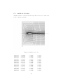
C.5 Airfoil for cfd codes
.
.
.
.
.
.
.
.
.
.
.
.
.
.
.
112
112
114
115
116
118
1
.
.
.
.
.
.
.
.
.
.
.
.
.
.
.
.
.
.
.
.
.
.
.
.
.
.
.
.
.
.
.
.
.
.
.
.
.
.
.
.
.
.
.
.
.
.
.
.
.
.
.
.
.
.
.
.
.
.
.
.
.
.
.
.
.
.
.
.
.
.
.
.
.
.
.
.
.
.
.
.
.
.
.
.
.
.
.
.
.
.
.
.
.
.
.
.
.
.
.
.
.
.
.
.
.
.
.
.
.
.
Introduction
This document is the description of CalculiX GraphiX (cgx). This program is
designed to generate and display finite elements (FE) and results coming from
CalculiX CrunchiX (ccx). If you have any problems using cgx, this document
6
should solve them. If not, you might send an email to the author [3]. The Concept and File Format sections give some background on functionality and mesher
capabilities. The Getting Started section describes how to run the verification
examples you should have obtained along with the code of the program. You
might use this section to check whether you installed CalculiX correctly. Then,
a detailed overview is given of the menu and all the available keywords in alphabetical order in the Menu and Commands sections respectively. Finally, the
User’s Manual ends with the appendix and some references used while writing
the code.
2
Concept
This program uses the openGL library for visualization and the glut library [2]
for window management and event handling. This results in very high speed
if a hardware-accelerated openGL-library is available and still high speed for
software-rendering (MesaGL,[1]).
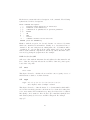
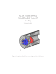
The cgx has pre- and post-processor capabilities. It is able to generate and
display beam, shell and brick elements in its linear and quadratic form (fig. 1).
In addition, it can display but not create pentahedra- and tetrahedra-elements.
The built-in mesher creates a structured mesh based on a description of
the geometry. For example, it uses lines for beam elements, surfaces for shell
elements and volumes (bodies) for brick elements. The program distinguishes
between the mesh and the underlying geometry. Elements are made from faces
and faces are made from nodes. If you move a node, the corresponding face(s)
and element(s) will follow. The geometry behaves according to the mesh: Lines
are made from points, surfaces are made from lines and bodies are made of
surfaces. Surfaces might have 3 to 5 edges and bodies might have 5 to 7 surfaces.
As a result, if you modify the position of a point, all related geometry will follow.
In other words, if the location of geometric entities is changed, it is necessary to
move the points on which the entities rely. It should be noted that faces exist
only on free surfaces of the model.
Even though cgx cannot generate tet-meshes, it is still possible to generate
a surface-mesh of triangles and export it in stl-format. This format can be read
by external meshers such as NETGEN [4]. This mesher fills the volume with
tetrahedra elements and is able to export the Abaqus file format. This can be
read by cgx and ccx (see also ”How to deal with cad-geometry”).
In addition, entities can be grouped together to make sets. Sets are useful
to handle parts of a model. For example, sets can be used to manipulate or
display a few entities at a time (see also ”How to define a set of entities”).
After a mesh is created in cgx, it needs written to a file for use with the solver.
Likewise, several boundary conditions and loads can be written to files (see also
”How to connect independent meshes”, ”How to define loads and constraints” and
”send”). These files need to be added into the control file for later use in ccx.
Additional commands, material description and so on must be added with the
help of an external editor.
7
After the analysis is completed, the results can be visualized by calling the
cgx program again in an independent session. The program is primary controlled
by the keyboard with individual commands for each function. Only a subset
of commands which are most important for post-processing is also available
through a pop-up menu. Shaded animations of static and dynamic results, the
common color plots and time history plots can be created. Also, a cut through
the model can be done which creates a section and it is possible to zoom through
the model.
Skilled users might include their own functions. For example someone may
need his own functions to manipulate the result-data or he may need an interface
to read or write his own results format (see also ”call”).
Both the pre- and post- processing can be automated in batch-mode (see
also ”How to run cgx in batch mode”).
3
File Formats
The following file-formats are available to write(w) and/or read(r) geometric
entities:
• fbd-format(r/w), this format consists of a collection of commands explained in the section ”Commands” and it is mainly used to store geometrical information like points, lines, surfaces and bodies. But it can
also be used to define a batch job which uses the available commands.
• step-format(r), reverse engineered based on some cad files. Only points
and certain types of lines are supported currently.
• stl-format(r/w), this format describes a shape using only triangles (see the
read command to handle edges generated by NETGEN).
Common CAD formats are supported by stand-alone interfaces which translate
into fbd-commands.
The following file-formats are available to write a mesh and certain boundaryconditions:
• Abaqus, which is also used by the CalculiX solver ccx.
• Ansys, most boundary conditions available.
• Code Aster, mesh and sets of nodes and elements are available.
• Samcef, mesh and sets of nodes and elements are available.
• dolfyn, a free cfd-code [5].
• duns, a free cfd-code [6].
• isaac, a free cfd-code [7].
8
• OpenFOAM, a free cfd-code [8], only 8-noded brick-elements are supported.
• Nastran, most boundary conditions available.
• tochnog, a free fem-code [9], only 8-noded brick-elements are supported.
The following solver-input-file-formats can be read to check the mesh, sets and
certain boundary-conditions:
• Abaqus, this is also used by the CalculiX solver ccx.
• Netgen, read Netgen native format (.vol)
The following file-formats are available to read solver results:
• frd-format, files of this format are used to read results of previous calculations like displacements and stresses. This format is described in section
”Result Format.” It is also used by ccx.
• duns, a free cfd-code [6],
• isaac, a free cfd-code [7],
• OpenFOAM, a free cfd-code [8].
For a more detailed description on how to use cgx to read this formats see
”Program Parameters” and the program specific ”Tips and Hints” sections. See
the ”send” command for how to write them from cgx.
4
Getting Started
For installation help, see .../Calculix/cgx X.X/INSTALL. After the program is
installed on your machine, you should check the functionality by running the
examples included in the distribution. The examples are located in .../Calculix/cgx X.X/examples/. Before going further, you should read the section
”Input Devices”. Then, begin with a result file called result.frd. Just type
”cgx result.frd”
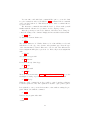
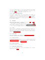
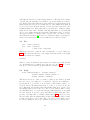
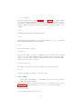
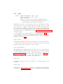
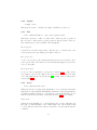
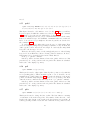
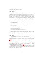
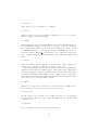
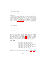
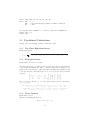
and some information is echoed in the xterm and a new window called main window appears on the screen. The name conventions used for the different areas
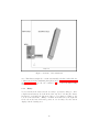
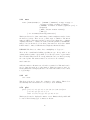
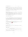
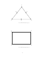
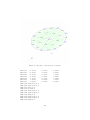
in the main-window are explained in figure 2. Now you should move the mouse
pointer into the menu-area and press the left mouse-button. Keep it pressed
and continue over the menu item “Dataset” to “Disp”. There you release the
button. Then press the left button again and continue over “Dataset” and “Entity” to “D1”. For background informations look into the subsection ”Datasets”
and ”Entity” which explains how to display results. After seeing the values you
might play around a bit with the ”Menu”. See also the commands ”steps”,
9
”max”, ”min”, ”scal” which might be used to modify the colour representation
of the displayed values. For example type “min 0” to change the lower value of
the colour bar. Watch out if you type a command; the cgx window MUST stay
active and not the xterm from which the program was started. It is better to
stay with the mouse pointer in the cgx window. Next, ”Quit” the program and
type
”cgx -b geometry.fbd”
in the xterm. The program starts again but now you see only a wire-frame
of the geometry. Move the mouse-pointer into the new window and type ”mesh
all”. The mouse-pointer MUST stay in this window during typing and NOT in
the xterm from which the program was started. After you see ”ready” in the
parent xterm, the mesh is created. To actually see it, type ”plus ea all”. Now
you see the mesh in green color. To see the mesh as a wire-frame, choose in the
main menu”Viewing” and continue to the entry ”Toggle Element Edges” and
then again in ”Viewing” choose ”Dots”. To see the mesh illuminated chose in the
main menu ”Viewing” and continue to the entry ”Show Elements With Light”.
To see it filled, choose in the main menu ”Viewing” and continue to the entity
”Fill”. Most of the time it is sufficient to see the surface elements only. For
this purpose, choose in the main menu ”Viewing” and continue to the entry
”Toggle Surfaces/Volumes”. If you start cgx in the post processor mode, as you
did in the first example (cgx result.frd), the surface mode is automatically set.
To see the interior of the structure, choose in the main menu ”Viewing” and
continue to the entity ”Toggle Culling Back/Front”. To save the mesh in the
format used by the solver, type ”send all abq”. To store the mesh in the result
format type ”send all frd”.
To create a new model start the cgx by typing
”cgx -b file”
where ”file” will be the name of the new model if you later exit the program
with the command ”exit”. The way to create a model from scratch is roughly
as follows, create
• points with ”qpnt” or ”pnt”,
• lines with ”qlin”,
• surfaces with”qsur”,
• Bodies with ”qbod”.
If possible, create higher geometry by sweeping or copying geometry with ”swep”
or ”copy”. The commands require sets to work with. Sets reference entities like
bodies or nodes. They are usefull because you can deal with a bunch of entities
at once. See the section ”How to define a set of entities” about how to create
them.
10
You can write a file with basic commands like ”pnt” to create the basis
for your construction and read it with the ”read” command. Most commands
can be used in batch mode. This allows the user to write a command file for
repeated actions.
The interactive commands start with the letter ’q’. Please make yourself
familiar with all of them before you start to model complex geometry.
After the geometry is created, the divisions of the lines can be changed to
control the density of the elements. Display the lines and their divisions with
• ”plot ld all”.
To change the element division, use
• ”qdiv”.
The default division is ”4”. With a division of”4,” a line will have 6 nodes and
will therefore be the edge of two element of the quadratic type. Next, the type
of the elements must be defined. This can be done for each of the different sets.
A new assignment will replace a previous one. Delete all previous assignments
with
• ”elty all”
and assign new types with
• ”elty all he20”.
If a mesh is already defined type
• ”del mesh”
and mesh again with
• ”mesh all”.
Then choose the menu entity ”Viewing - Show Elements With Light” to see the
mesh lighted. Lastly, export the mesh in the calculix solver format with
• ”send all abq”.
With the ”send” command, it is also possible to write boundary conditions,
loads and equations to files. The equations are useful to ”glue” parts together.
It is advisable to save your work from time to time without exiting the program. This is done with the command
• ”save”.
You leave the program either with
• ”exit”
or with
11
• ”quit”.
Exit will write all geometry to an fbd-file and if a file of this name exists already
then the extension of this file will be renamed from fbd to fbb. ”quit” closes
the program without saving.
A solver input file can be written with the help of an editor (emacs, nedit
etc.). If you write a ccx command file, then include the mesh, the boundary
conditions etc. with the ccx command ”*INCLUDE”. After you finished your
input-file for the solver (ccx) you might read it by calling the program again with
”cgx -c solverfile.inp”
for a final check. All predefined sets are available together with automatically generated sets which store boundaries, equations and more. These sets
start with the ”+”-sign. For example the set +bou stores all constrained nodes
where the set +bou1, +bou2, +bou3 store the constraints for the individual directions. Further the set +dep and +ind store the dependent and independent
nodes involved in equations etc. See which sets are defined with the command
• ”prnt se”.
Each line starts with the set-index, then the set-name followed by the number of
all referenced entities. The sets can be specified by index or name. For example
if the index of set ”blade” is ”5” the following commands are equivalent:
• ”plot p 5”
• ”plot p blade”
Predefined loads are stored as ”Datasets” to be visualized. Sets with the name
of the load-type (CLOAD, DLOAD) store the related nodes, faces or elements.
Use the command
• ”plot”
or
• ”plus”
to visualize entities of sets.
Then run the input file with ccx. The result file (.frd) can be visualized with
”cgx filename.frd filename.inp”
were the solver input file ”filename.inp” is optional. With this file, the sets,
boundary conditions and loads used in the calculation are available together
with the results.
If you have problems doing the above or if you want to learn more and in more
detail about the cgx continue with the tutorial [10] and look in the appendix,
section Tips and Hints and Known Problems.
12
5
Program Parameters
usage:
cgx [-a|-b|-bg|-c|-duns2d|-duns3d|-isaac2d|-isaac3d|-foam|-ng|-step|-stl]->
filename [ccxfile]
-a
-b
-bg
-c
-duns2d
-duns3d
-isaac2d
-isaac3d
-foam
-ng
-step
-stl
[-v]
automatic-build-mode, geometry file derived from a
cad file is expected
build-mode, geometry file in fbd-format is expected
background, suppress creation of graphic output
otherwhise as -b, geometry (command) file must be provided
read an solver input file (ccx, Abaqus)
read duns result files (2D)
read duns result files (3D)
read isaac result files (2D)
read isaac result files (3D)
read the OpenFOAM result directory structure
read Netgen native format (with surface domains)
read an ascii-step file (points and lines only)
read an ascii-stl file (triangles)
(default) read a result file in frd-format and optional
a solver input file (ccx) in addition which provides the
sets and loads used in the calculation.
special purpose options:
-mksets
make node-sets from *DLOAD-values (setname:’’_<value>’’)
-read
forces the program to read the complete result-file
at startup
If no option is provided then a result-file (frd) is assumed, see ”Result Format”.
A file containing commands or geometric informations is assumed if the
option -b is specified. Such a file will be created if you use ”exit” or ”save” after
you have interactively created geometry. Option -a awaits the same format
as option -b but merging, defining of line-divisions and the calculation of the
interior of the surfaces is done automatically and the illuminated structure is
presented after startup. This should be used if the commandfile was generated
by an interface-program which convertes cad-data to cgx-format (for example
vda2fbd). With option -a and -b the program will start also if no file is specified.
An input file for the solver can be read with option -c. Certain key-words are
known and the affected nodes or elements are stored in sets. For example the
default set(s) +bou(dof) store nodes which are restricted in the corresponding
degree of freedom and the set(s) +dep(dof) and +ind(dof) store dependent and
independent nodes used in equations.
A special case is OpenFOAM. The results are organized in a directory structure consisting of a case containing time-directories in which the result-files are
stored. The user must call cgx using the case-directory (cgx -foam case). The
13
program will then search the time-directories. The time directories must contain a time-file to be recognized. Or in other words each directory in this level
containing a time-file is regarded as a result directory.
6
6.1
Input Devices
Mouse
The mouse is used to manipulate the view-point and scaling of the object inside
the drawing area (figure 2). Rotation of the object is controlled by the left
mouse button, zoom in and out by the middle mouse button and translation of
the object is controlled by the right mouse button. Inside the menu area, the
mouse triggers the main menu with the left button.
In addition the mouse controls the animation of nodal values. The animation
will stop if the mouse pointer is not in the drawing area but will start again
if the pointer enters the drawing area. This can be prevented by pressing the
middle mouse button while the mouse pointer is in the menu area. Pressing the
right button will release the next frame. A frozen animation can be released
by pressing the middle button. The previous frame can be reloaded by pressing
the middle mouse button twice and the right button once (while the mouse is
in the menu area).
6.2
Keyboard
The Keyboard is used for command line input and specifying the type of entities
when selecting them with the mouse pointer. The command line is preferable
in situations where pure mouse operation is not convenient (i.e. to define a
certain value) or for batch controlled operations. Therefore most commands are
only available over the command line. The stream coming from the keyboard
is echoed in the parent-xterm but during typing the mouse pointer must stay
inside the main window. Otherwise the commands will not be recognized by
the program.
The following special keys are used:
Special Keys:
ARROW_UP:
previous command
ARROW_DOWN: next command
PAGE_UP:
entities of previous
plot or plus) or the
PAGE_DOWN: entities of next set
plot or plus) or the
14
set (if the last command was
previous Loadcase
(if the last command was
next Loadcase
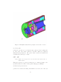
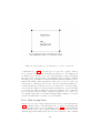
Figure 2: structure of the main-window
7
Menu
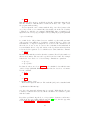
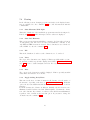
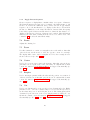
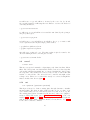
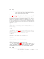
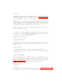
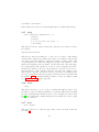
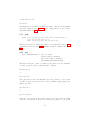
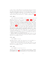
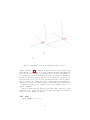
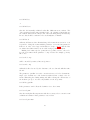
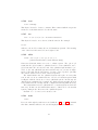
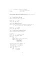
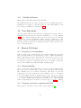
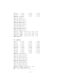
The main menu pops up when pressing the left mouse-button inside the menuarea (figure 3). It should be noted that there are equivalent command-line
functions for most of the menu-functions. This can be used for batch-controlled
post-processing. Next the entities inside the main menu will be explained:
7.1
Datasets
Datasets are selected with the menu-item ”Dataset”. A dataset is a block of
nodal values. These could be displacements due to a linear analysis or for
a specific time-step during a nonlinear analysis. It could also contain other
values like stresses, strains, temperatures or something else. To select a dataset,
make sure that the mouse-pointer is inside the menu area. Then, press the left
mouse button and move the mouse-pointer over the menu entry ”Dataset”, then
continue to the right. A sub-menu pops up showing all available datasets with
a leading number and sometimes followed by a dataset-value (usually time or
frequency) and a dataset-description. Move the mouse-pointer over a dataset
you are interested in and release the left mouse button. The dataset is now
selected. A results ”Entity” must be chosen to see the values in the drawing-
15
Figure 3: structure of the main-menu
area. This Dataset might also contain automatically calculated values like the
v. Mises stress and the maximum principal stress (see Pre-defined Calculations
and Result Format). See also the command ”ds” to control the functionality
with the command-line.
7.1.1
Entity
To view data from the dataset, its also necessary to specify the entity (i.e. dx for
a displacement Dataset). It works in the same way as for selecting the dataset
but instead of releasing the left mouse button over a Dataset continue to the
bottom of the sub-menu to ”Entity.” Continue from that item to the right and
release the mouse button when the pointer is over an entity. Now the data is
displayed in the drawing-area.
16
7.2
Viewing
In the following sections, changing properties and styles of the displayed structure are explained. See the command ”view” to control the functions with the
command-line.
7.2.1
Show Elements With Light
This is the default view of the mesh if the program was started in viewing mode.
If used, any animation will be interrupted and no values are displayed.
7.2.2
Show Bad Elements
This option presents elements which have a negative Jacobian value at least at
one integration point. The solver ccx can not deal with those elements. So far,
only TET and HEX elements are checked. These elements are stored in the set
called -NJBY. See also the command ”eqal”.
7.2.3
Fill
This is the default mode and forces the element faces to be rendered.
7.2.4
Lines
The edges of the element faces are displayed. This is especially useful to see into
the structure to find hot spots in the displayed field. With ”Toggle Move-Z/Zoom”
and ”qcut”, a more detailed analysis can follow. For very dense meshes switch
to ”Dots”.
7.2.5
Dots
The corners of the element faces will be displayed. This is especially useful if
values inside the structure need checked.
7.2.6
Toggle Culling Back/Front
This removes the faces of volume elements for all elements or for the surface of
the structure, depending on the state of ”Toggle Surfaces/Volumes”. With this
option, the user can visualize internal structures like cracks or a core of a hollow
structure.
For shell elements, the behavior is different. Initially only the front faces are
illuminated and the back faces are dark. This is helpful to determine the orientation of the elements. If you want to see all faces of the shell-elements illuminated
regardless of the orientation, then use this option. If you want to change the
orientation use the command ”qflp”.
17
7.2.7
Toggle Model Edges
Per default, all free element edges are shown. The user can remove/show them
with this option.
7.2.8
Toggle Element Edges
Per default, just the free element edges are shown. The user might add all edges
to the structure with that option.
7.2.9
Toggle Surfaces/Volumes
This switches the way each volume elements are displayed. Either all faces
of the elements or just the element faces on the surface of the structure are
displayed. Depending on the state of ”Toggle Culling Back/Front,” either the
faces pointing to the user or the faces pointing away are displayed. The default
is just to show the surface pointing to the user. In the lower left corner of the
drawing area,(see figure 2) a character is printed, indicating the program is in
the surface mode ”s” or in the volume mode ”v”.
7.2.10
Toggle Move-Z/Zoom
Instead of zooming in with the help of the middle mouse button, it is also
possible to move a clipping plane through the structure to get a view of the
inside. The clipping plane is parallel to the screen and will be moved in the
direction to and from the user by pressing the middle mouse button and moving
the pointer up and down while inside the drawing area. Usually it needs some
mouse movements until the clipping plane has reached the structure. Depending
on hardware, this functionality could be slow. After zooming in, consider using
the ”plot” and ”plus” commands to customize your view.
7.2.11
Toggle Background Color
With this option, it is possible to switch between a black and a white background.
7.2.12
Toggle Vector-Plot
It is possible to add small ”needles” to the plot which point with their heads
in the direction of the vectors. Only entities which are marked in the database
as vectors will be affected. See ”Nodal Results Block” for information on how
entities are marked as vectors. Internally calculated vector-results, like the worst
principal stress, are marked automatically. If one component or the value of a
vector is selected, then the option takes immediate effect.
This option can be used in combination with ”Animate Toggle Dataset Sequence”.
See also the keyboard command ”ds” how to select datasets and entities with
the keyboard. In this case, entities which are NOT marked in the dataset as
18
vectors can be displayed with vector-needles. This command line approach with
”ds” is the only way to display duns-cfd-results with vector-needles. See also
the command ”scal” how to manipulate the length of the vectors.
7.2.13
Toggle Add-Displacement
It is possible to display results on the deformed structure. For example, you
can display a stress field on the deformed structure. If you know a suitable
amplification factor for your displacements then use the ”scal” command to
issue this value but this can also be done later. Of course displacements for the
Loadcase must be available.
7.3
Animate
This option allows the animation of displacements. See also ”ds” and ”scal” to
use this functionality with the command-line.
It is possible to create this sequence from just one Dataset, see ”Start”.
This is useful for displaying mode-shapes. See also ”Toggle Dataset Sequence”
to create a sequence from multiple Datasets to visualize dynamic responses.
7.3.1
Start
Creates a sequence of display-lists to visualize displacements (for example modeshapes). The program recognizes displacements just by the name of the dataset.
This name must start with the letters ”DISP”, otherwise the animation will not
start (see ”Nodal Results Block”).
7.3.2
Tune-Value
Controls the amplitude of the animation. If ”Toggle Real Displacements” was
chosen before, the tune-value is equivalent to the amplification of the animation.
7.3.3
Steps per Period
Determines how many display lists for one period of animation will be used. If
”Toggle Dataset Sequence” was chosen, then these number of display lists will
be interpreted as one period (see Time per Period).
7.3.4
Time per Period
Determines how many seconds per period.
7.3.5
Toggle Real Displacements
To see the correct displacement of each node. The animation can be controlled
with the help of the mouse.
19
7.3.6
Toggle Dataset Sequence
Creates a sequence of display-lists to visualize values of a sequence of Datasets.
The Datasets must use the same type, for example only displacements or only
stresses. To activate the animation, after you have selected “Toggle Dataset
Sequence” choose the first Dataset to be displayed, then the second and then
the last one. Finally choose the entity. The first two datasets define the spacing
between the requested datasets and the third-one defines the last dataset to be
displayed. The last two selections of datasets can be omitted. Then all datasets
which use the same name, starting from the selected one, will be used. The
command ”ds” provides the same functionality.
7.4
Frame
Adjusts the drawing box.
7.5
Zoom
Use this command to zoom into a rectangular section of the window. After this
option is chosen, use the mouse to select the opposite corners of a rectangle.
The display will zoom in on the rectangular area. Note the rectangle is never
shown on the screen (see also ”zoom”).
7.6
Center
Used to choose a new center point for the structure. After this option is chosen,
pick either a node, a point or the corner of an entity. To easily find the element
corners, the function ”Toggle Element Edges” is triggered automatically (see
also ”qcnt”).
7.7
Enquire
Used to investigate parameters like the value and the position of a certain node
of the model. Pick a node after this option is chosen. To easily find the element
corners, the function ”Toggle Element Edges” is triggered automatically (see
also ”qenq”).
7.8
Cut
Used to cut elements and to create a section of new elements and nodes. Either
pick three nodes, or, in case a dataset-entity of a vector was already selected,
use the menu entry “vector” and select just one node. The cutting plane is then
determined by the direction of the vector (displacements, worstPS). To easily find the element corners, the function ”Toggle Element Edges” is triggered
automatically (see also ”qcut” and ”cut”)
20
7.9
Graph
Used to generate a 2D-plot. The option “Length” will provide a plot “value
over distance between nodes”. The option “Datasets” will provide a plot “value
over Dataset-nr” and the option “Time” will provide “value over Time”. For
the later two options it is necessary to first create an animation with either the
command ”ds” or the menu option ”Toggle Dataset Sequence” (see also ”graph”
and ”How to generate a time-history plot”). To easily find the element corners,
the function ”Toggle Element Edges” is triggered automatically.
7.10
7.10.1
Orientation
+x View
To look along the x-axis.
7.10.2
-x View
To look against the x-axis.
7.10.3
+y View
To look along the y-axis.
7.10.4
-y View
To look against the y-axis.
7.10.5
+z View
To look along the z-axis.
7.10.6
-z View
To look against the z-axis.
7.11
Hardcopy
To create a hard-copy during animation, it is useful to stop the animation first
with the middle mouse button while inside the menu area of the main window
and then release one picture after the other with the right button until the
desired amplitude or step is reached.
7.11.1
Tga-Hardcopy
To create a window dump in tga format. You might use the program ”convert”
[11] to convert this format to others.
21
7.11.2
Ps-Hardcopy
To create a window dump in postscript format. The program convert must be
installed.
7.11.3
Gif-Hardcopy
To create a window dump in gif format. The program convert must be installed.
7.11.4
Png-Hardcopy
To create a window dump in png format. The program convert must be installed.
7.11.5
Start Recording Gif-Movie
All frames during an animation are stored. The recording ends after the right
mouse button is pressed while in the menu area. Finally all frames are combined
in the file ”movie.gif” which can be displayed with various tools (Firefox [12] or
realplay). If the animation is stopped with the middle mouse button while in
the menu area, then the movie stops until it is released by pressing the middle
mouse button again. See ”movi” for the keyboard options. Further remarks in
”How to change the format of the movie file”.
7.12
Help
Starts the html help and displays this document. It only works if the specified
html-viewer is available. The default is Firefox [12] but this can be changed
in the ”cgx.h” file. The search-path for the documentation is also defined in
the ”cgx.h” file. Please make sure that the documentation is in the specified location or change the path in the ”cgx.h” file and recompile the program after the object-files are deleted. The default location for the html help
is .../CalculiX/cgx X.X/doc/cgx and /CalculiX/ccx X.X/doc/ccx for cgx and
ccx respectively. The html files must be downloaded directly or compiled from
the latex source for this function to work properly. The INSTALL file tells
how to compile the latex code to html. The INSTALL file is located .../CalculiX/cgx X.X/ and .../CalculiX/ccx X.X/ for cgx and ccx respectively.
7.13
Quit
This terminates the program without a save.
8
Commands
This section is a reference to all commands and their parameters in alphabetic
order. If a command is typed the mouse-pointer must be in the main window
(figure 2). Only the echo of the input stream is visible in the parent xterm. The
keywords are not case sensitive but all command parameters are case sensitive.
22
Each reference starts with a short description of the command. The following
syntax is used for these descriptions:
Known commands and syntax:
’..’:
Keyword (either uppercase or lowercase)
<..>:
Parameter (case-sensitive)
[..]:
combination of parameters or optional parameter
(..):
Remark
|
:
OR
&
:
AND
:
from-to
-> :
command continues in the next line
RETURN press the RETURN key
Entities—with the exception of nodes and elements—are referenced by names
which can contain letters and numbers. Usually one to four characters is recommended. If a new entity uses an existing name, the old definition will be
overwritten. To overcome this problem, ”alias” names can be used. An alias
name is defined with the ! sign in front. An already defined alias name can be
referenced by placing the % sign in front. For example:
LINE !L1 %P1 %P2 %SET
will create a line with the alias name L1 and will use the alias names P1 and
P2 to define the end-points and uses the set SET to define the point sequence
between the end-points.
8.1
area
’area’ <set>
This keyword is used to calculate the area and the center of gravity of a set of
shell-elements or surfaces of volume-elements.
8.2
asgn
’asgn’ ’n’|’e’|’p’|’l’|’c’|’s’|’b’|’S’|’L’|’se’|->
’sh’|’alpha’|’beta’|’nadapt’ <value>
This keyword is used to define the first node or element number which will be
used for the next mesh generation. And it is used to redefine the leading character of new entities. The default is D for points p, L for lines l, C for combined
lines (lcmb) c, A for surfaces s, B for Bodies b, Q for nurb lines (nurl) L, N for
nurb surfaces (nurs) S, A for sets se and H for Shapes sh. For example
asgn p U
23
will assign the character U as the leading character to all newly created names
of points. The automatically created names of geometric entities use 4 characters. If all possible names with the chosen leading letter are in use then the next
alphabetical letter is chosen as a leading letter, so after PZZZ follows Q000. If
no more letter follow then the amount of letters per name is increased. The
maximum number is 8. Each entity has its own name-space. Different entities
might use the same name. Remark: Currently nurbs-lines are automatically
used to create splines sharing the same name. Nurbs-lines can not be used for
other purposes than to be displayed and so far they can not be written to a file.
The unstructured mesher [14] uses the tree parameters alpha, beta, nadapt for
mesh-control. Current default is 0.4 for alpha and beta and 4 for nadapt.
8.3
bia
’bia’
’bia’
<line> [<bias>]|
<set> [<bias>]|
[’mult’|’div’ <factor>]]
This keyword is used to define the bias of a single line or of a set of lines (see
qadd). The bias defines the ratio of the length of the first element to the length
of the last element. For example,
bia all 4.5
will force a ratio in which the last element is 4.5 times bigger than the first
one. Real numbers are permitted since version 1.5 (see also qbia). To convert
from pre 1.5 versions, start the program with the -oldbias option.
8.4
body
’body’ <name(char<9)>|’!’ [<surf1> <surf2>]|
[<surf1> <surf2> <surf3> <surf4> ->
<surf5> [<surf6> <surf6>]]
This keyword is used to define or redefine a volume (body). Each body must
have five, six or seven surfaces to be mesh-able. However, it is sufficient to
specify just the ”top” and the ”bottom” surfaces. But if surfaces with 3 or 5
edges are involved then this surfaces have to be the ”top” and ”bottom” surfaces. This is also true if surfaces have different line-divisions at opposite edges.
The missing surfaces between the ”top” and ”bottom” surfaces will be created
automatically if they do not already exist (they will always have 4 edges with
the same division on opposide edges). But all needed lines must exist. More
precisely, only single lines or existing combined lines (lcmb) can be detected.
The user must define the missing surface if just a chain of lines (and no lcmb)
is defined between two corner points of the ”top” and ”bottom” surfaces before
he can successfully use the body command. It is a more convenient way to
24
define a body than the command “gbod” but exactly 2 or all surfaces must be
specified otherwise the body will not be created (The most convenient way to
define bodies is to use the command “qbod”). For example,
body b1 s1 s2
will look for the missing surfaces and if necessary create them if all lines between
the corner points of s1 and s2 are defined; the result is the creation of body, b1.
Or for example,
body ! s1 s2 s3 s4 s5
will create a body and a new name for it. The new name is triggered by the
sign !. Here the body is based on 5 surfaces. If the surfaces are not connected,
the body is not mesh-able.
8.5
call
’call’ <parameters>
This keyword is used to allow the user to control his own functionality in the file
”userFunction.c”. The data-structures for the mesh and datasets are available.
The default function calculates the hydrodynamic stresses with the command:
call hydro
See ”User-Functions” for details.
8.6
cntr
’cntr’ <pnt|nod>
Defines a new center-point or -node. This command is intended for batch-mode.
See also ”qcnt” for the cursor controlled command.
8.7
comp
’comp’ <set|*chars*> ’u’|’d’|’e’
This keyword is used to add all entities to the specified set (see seta) which depend on the already included entities (u, up), or to include all entities necessary
to describe the already included entities (d, down).
For example the set ”lines” stores lines and should also include all dependent
points:
comp lines do
25
Or the set ”lines” should also include all surfs and bodies which depend on
the lines:
comp lines up
In some cases you will need only the end-points of lines. With the option
(e, edges)
comp lines e
only end-points are included in the set. One exception to this logic was introduced for convenience:
comp nodes do
will add all faces described by the nodes in set nodes despite the fact that
faces are made from nodes.
Wildcards (*) can be used to search for setnames of a certain expression:
comp E* do
will complete all sets starting with “E”.
8.8
copy
’copy’ <set> <new_set> [’scal’ <fx> <fy> <fz> <pnt> [a] ]|
[’tra’ <dx> <dy> <dz> [a]]|
[’rot’ <p1> <p2> <alfa> [a] ]|
[’rot’ ’x’|’y’|’z’|’p’<PNT> <dr> [a] ]|
[’rad’ <p1> <p2> <alfa>]|
[’rad’ ’x’|’y’|’z’|’p’<PNT> <dr> [a] ]|
[’mir’ <P1> <P2> [a] ]
This keyword is used to create a copy of a set (see seta about sets). Geometry,
nodes and elements with their results can be copied. The copy of results is
usefull to evaluate additional sectors in case of a cyclic symmetric calculation.
The copy is included in the new set. Existing sets are extended by the copied
entities if the last parameter “a” (append) is provided. Several transformations
are available. For example scal creates a scaled copy, the scaling factors fx, fy,
fz can be chosen independently,
Several transformations are available. For example scal creates a scaled copy,
the scaling factors fx, fy, fz can be chosen independently,
copy part1 part2 scal 2 P0
copy part1 part2 scal 1 1 2 P0
26
tra will create a copy and will move it away by the vector dx, dy, dz and
the optional parameter a will assign the new entities to sets were the mother of
each entity is included,
copy set1 set2 tra 10 20 30 a
rot will create a copy and will move it around the axis defined by the points p1
and p2 by alfa degrees,
copy set1 set2 rot p0 px 20.
rad will create a copy and will move it radially to the x-, y- or z-axis or will
create a spherical section if just a single point is defined,
copy cylinder1 cylinder2 rad x 20.
copy sphere1 sphere2 rad pP0 10.
mir will create a mirrored copy. The mirror-plane is placed normal to the
direction running from P1 to P2 and placed at P2,
copy section1 section2 mir P1 P2.
8.9
corrad
’corrad’ <set>
This is a very special command to adjust improperly defined arc-lines, like in
fillets. The center points of arc-lines included in the set are moved in a way that
each arc-line will run tangentially into a connected straight line. But because
the end-points of the arc-lines are not moved only one side of each arc-line will
run into a connected line. The other side is not controlled and might end in
a sharp corner. Therefore for each arc-line exactly one connected straight line
must be included into the set (figure 4).
8.10
cut
’cut’ <pnt|nod> [<pnt|nod> <pnt|nod>]
This keyword is used to define a cutting plane through elements to visualize
internal results. The plane is either defined by three nodes or points, or, in
case a dataset-entity of a vector was already selected, by just one node or point.
The cutting plane is then determined by the direction of the vector (displacements, worstPS). The menu option ”Show Elements With Light” or the commands ”ucut”, ”view surf” or”view volu” will display the whole model again and
will delete the plane. This command is intended for batch-mode. See ”qcut”
for the cursor controlled command.
27
Figure 4: Effect of the corrad command
8.11
del
’del’ [’p’|’l’|’l0’|’c’|’s’|’b’|’t’|’S’|’L’|’se’|’sh’ <entity>]|
[’se0’]|
[’mesh’]|
[’pic’]
This keyword is used to delete entities, the whole mesh (see also qdel) or a
background-picture. For example,
del se part
will delete the set “part” but all included entities are untouched. The following
entities are known:
Points p, Lines l, Combined Lines c, Surfaces s, Bodies b, Node Texts t, Nurb
Surfaces S, Nurb Lines L, Sets se and Shapes sh.
When an entity is deleted, all dependent higher entities are deleted as well.
Special cases are
del l0 set (l¡zero¿)
were all lines with zero length in set ”set” are deleted and
28
del se0
will delete all empty sets. If a background-picture was loaded with the ”read”
command it can be deleted with:
del pic
8.12
div
’div’
’div’
<line> [<division>]|
<set> [<division>]|
[’mult’|’div’ <factor-div> <factor-bias>]|
[’auto’ <node-dist> <angle>]
This keyword is used to define the division of line(s). The div keyword also
works on a set of lines (see qadd). The division controls the number of nodes
created when the geometry is meshed (see elty and mesh). For example,
div all 4
attaches the division of 4 to all lines. With the keyword mult or div in combination with a value, it is possible to multiply or divide already assigned divisions:
div all mult 2.
Or in case you need a starting-point for the individual divisions you can use
the option auto with the optional parameters node-dist and angle. Node-dist
is the maximum allowed distance between nodes and angle is the maximum allowed angle defined by three sequential nodes. If one parameter is not fulfilled
then the division is halved. Default values are defined in the file cgx.h
div all auto
Some rules must be fulfilled before a geometry is meshable. For linear elements (ie. qu4 or he8), the sum of all divisions of each surface must be even.
In case of quadratic elements (ie. qu8 or he20) this sum must be divisible by
4 without residue. Opposite edges of a given surface might have different divisions. For example on the left side of a given surface the division is 8 and on
the right side it is only 4. But only two opposite surfaces of a body can use this
feature. These surfaces are called top and bottom surfaces. All other surfaces
of this body must have unique divisions on opposite edges.
8.13
ds
’ds’ <1.Dataset-Nr> <2.Dataset-Nr> <n.Dataset-Nr> ’a’|->
[’e’ <entity-nr> (up to 4 times)]|
29
[’s’ <value>]
This keyword is used to define a Datasets and an Entity. The Dataset might
be a positive number which has to match the nr in the Dataset-menu or an ’l’
(lower case ’L’) which is interpreted as the last available Dataset or a negative
number. Then it is interpreted as the last minus the specified number. For
example
lc 1 e 1
will display the first entity of the first Dataset.
lc l e 1
will display the last Dataset. To start the animation of the second-to-last
Dataset (assuming displacements) right away:
lc -1 a
Also sequences can be defined:
lc 2 4 10 e 1
Here the 1st entity of each second Dataset is selected. The selection starts
at the second- and ends at the 10th dataset. If more than one entity is defined
then a vector-plot will be displayed. If a 4th entity is defined then this entity
will be used for the basic color-plot:
lc 2 4 10 e 12 13 14 15
In addition, it is possible to scale the entities of the specified datasets:
lc 1 s 1.2
will scale all entities of dataset 1 by a factor of 1.2.
8.14
elem
’elem’ <nr> <firstNode> .. <lastNode> ’be2’|’be3’|’tr3’|’tr6’|->
’qu4’|’qu8’|’he8’|’he20’
This keyword is used to define elements based on nodes and its type (see section
Element Types in the appendix for the correct node-order). For example,
elem 1 1 2 3 4 qu4
creates a shell element with four nodes.
30
8.15
elty
’elty’ <set> ’be2’|’be2d’|’be3’|’tr3’|’tr3u’|’tr3e’|’tr3s’|->
’tr3c’|’tr6’|’tr6e’|’tr6s’|’tr6c’|’qu4’|’qu4e’|->
’qu4s’|’qu4c’|’qu8’|’qu8e’|’qu8s’|’qu8c’|’he8’|->
’he8f’|’he8i’|’he8r’|’he20’|’he20r’
This keyword is used to assign a specific element type to a set of entities (see
section Element Types in the appendix). The element name is composed of
the following parts: The leading two letters define the shape (be: beam, tr:
triangle, qu: quadrangle, he: hexahedra), then the number of nodes and at
last an attribute describing the mathematical formulation or other features (c:
axisymmetric, e: plain strain, s: plain stress, u: unstructured mesh, r: reduced
integration, i: incompatible modes, f: fluid element for ccx). If the element type
is omitted, the assignment is deleted. If all parameters are omitted, the actual
assignments are posted:
elty
will print only the sets with assigned elements. Multiple definitions are possible. For example,
elty all
deletes all element definitions. If the geometry was already meshed, the mesh
will NOT be deleted. If the mesh command is executed again after new assignments has taken place, additional elements will be created.
elty all he20
assigns 20 node brick-elements to all bodies in the set all.
elty part1 he8
redefines that definition for all bodies in the set part1.
elty part2 qu8
assigns 8 node shell elements to all surfaces in set part2.
Be aware of the command “mids” to remove or include mid-side nodes of
elements. Especially if you use the unstructured element-type tr3u. In this case
you might change the linear triangles to tr6 elements with this command.
8.16
enq
’enq’ <set> <set> [’set’ <setname> ]| ->
[’rec’ <x-value>|’_’ <y-value>|’_’ <z-value>|’_’ ]| ->
31
[’cyl’ ’x’|’y’|’z’ <r-value>|’_’ <axis-value>|’_’ ] ->
’tol’ ’i’|’a’|’h’|’l’ [<value>]
This command is used to locate entities from a certain set (first provided set)
and stores them in the second set. The following entities are handled: nodes,
points, lines, surfaces. But surfaces can only be identified if the command “rep
<setname>” was issued before. In case of nodes with related values (results)
it will also determine the highes or lowest value in the specified range, or, all
nodes above or below a certain value. The coordinates might be taken from one
node or point in a given 3rd set or given in cartesian coordinates (option rec)
or cylindrical coordinates (option cyl). Some coordinates might be omitted to
specify an infinite range. The ’ ’ key has to be used in this case. The mode
is defined by the keys ’i’ individual, ’a’ all, ’h’ high, ’l’ low, were h and l will
search the highest or lowest value in range. This value will also be written to a
file for automatic processing purposes. For example
enq all newset rec 10.
100. 0.1 i
will search for entities in set ’all’ at the given location x:10. y: (infinite range,
triggered by the ’ ’ key) z:100. with a tolerance of 0.1 and only the closest entity
of all kinds of entities are stored in set ’newset’, triggered by the ’i’ key. With
the ’a’ key all in range would be stored. The key ’h’ or ’l’ would trigger a search
for the highest or lowest value in the specified range.
In combination with a certain value
enq all newset rec 10.
100. 0.1 h 1013.
all nodes with a value above “1013.” would be stored in set “newset”. The
command
enq domain1 newset cyl x 100. 10. 0.1 a
will search for entities in set ’domain1’ at radius:100. around x at x:10. with a
tolerance of 0.1. All entities in range are stored in set ’newset’.
The following example illustrates the use of “enq” to find the highest value
close to a location given by a node-number:
# activate dataset 3 with entity 7:
ds 3 e 7
# read a file with one node to define a set:
read pos1.frd pos1
# search the highest value around a radius of 1:
enq all t set pos1 1. h
# move the file with the search result to a meaningfull name:
sys mv enq_lc3_e7_1.out pos1.out
32
8.17
eqal
’eqal’ ’jbir’|’aspr’|’mca’ <value>
The keyword without parameters lists the current element quality thresholds
(0==off):
• JBIR: The maximum ratio of jacobian determinants xsj between all gauspoints. Were xsj = Vworldcoordinates / Velementcoordinates and jbir =
xsj-max / xsj-min.
• ASPR: Element aspect ratio between all element sides.
• MCA: Maximum corner angle between all element sides.
With parameter “value” sets the value of the threshold.
8.18
exit
’exit’
This command terminates the program and saves the geometry (if any) to a file
named as the input file but with the extension .fbd. If a file with that name
exists already, then this file will be saved with the new file extension .fbb as a
backup (see also save).
8.19
flip
’flip’ <setname>|<surf> [’auto’]
This command changes the orientation of a set of surfaces or a single surface.
In case of a single surface with the parameter “auto” all surfaces will be flipped
in a way that they share a common direction (in or out of a volume). See also
qflp.
8.20
flpc
’flpc’
This command changes the colour of the scale. Initialy the default is red for
high values and blue for low values. The command will invert the current state.
8.21
font
’font’ ’d’|’l’ <value(1-6)>
33
This command changes the drawing-font. Six fonts of different heigh are available:
font d 6
selects the highest font for the drawing area were
font l 1
selects the smallest one for the legend. The default is selected if no number
is specified:
font d or font l
8.22
frame
’frame’
This command fits the model into the drawing area.
8.23
gbod
’gbod’ <name(char<9)>|’!’ ’NORM’ ’+|-’ <surf> ’+|-’ <surf> ->
.. ( 5-7 surfaces )
This keyword is used to define or redefine a body in the most basic way (see also
“qbod”). Each body must have five to seven surfaces to be mesh-able. However,
the number of recommended surfaces is six. The first two surfaces should be
the ”top” and the ”bottom” surfaces. For example,
gbod B001 NORM - S001 + S002 - S005 - S004 - S003 - S006
will create a body B001. The keyword ”NORM” is a necessary placeholder
for future functionallity but has no actual meaning. Next, follow the surfaces
with a sign ”+” or ”-” in front that indicates the orientation of each surface.
These signs will be corrected automatically if necessary. If the an automatically
generated name is desired, then type ”!” instead of a name.
8.24
gonly
’gonly’ ’on’|’off’
This keyword is used to erase the contents of the menu area. Sometimes this is
useful for hardcopies.
34
8.25
graph
’graph’
[<amplitude|*chars*> ’amp’ [’l’]]|
[<material|*chars*> ’mat’ [’l’]]|
[<seq> ’length’]|
[<set>|’-p’ ’nr’|’time’|’descr’|<parameter-name> ->
[<Dataset-name> <entity-name>|<parameter-name> ] ->
[<first-Dataset-Nr> <last-Dataset-Nr>] ]
This keyword is used to create time history plots of nodal values. The values
of the pre-selected nodes stored in the referenced set will be written to a file
called ”graph.out”. A gnuplot command file will be written called ”graph.gnu”
and executed. The resulting file ”graph.ps” will be automatically displayed with
the postscript viewer. The default is ”ghostview” but this can be changed in the
”cgx.h” file before the program is build. See also “How to generate a time-history plot”
for further details.
A set with the nodes of interest must be created (usually with “qadd”) before a graph can be drawn. If the parameter l (length) is used to plot values
along the length of a set of nodes then this set has to be of the sequence type
(usually created with “qseq”):
graph seq length
The length is calculated as the sum of the distances between successive nodes.
Since version 1.8, there are two ways of operation. One way is to specify the
Datasets and the entity as parameters of the command
graph set time DISP D1
which will display the displacement D1 of nodes in ”set” vs. the dataset-time of
all ”DISP” Datasets. The first and the last dataset can be specified optionally.
For the traditional way, a sequence of datasets must have been selected (see
Toggle Dataset Sequence). After the selection of the datasets, an Entity must
be specified. Then, the user could use the graph command to generate the
history-plot of this pre-defined sequence. The command
graph set nr
will display the values on the node-positions vs. the dataset-numbers. The
command
graph set time
will display the values on the node-positions vs. the dataset-values (usually time
or frequency, see Nodal Results Block, parameter “VALUE”)) and the command
35
graph set descr
will display the values on the node-positions vs. the dataset-description (only
makes sense if the description is a numerical value. See Nodal Results Block),
parameter “TEXT”, for the location of this data in the frd-file.
In addition, a second data-file is written ”graph.out2” which stores the nodenumber and the node-coordinates and all values at this node-position for all
datasets. This file can be used to display values over node-positions, etc. It is
up to the user to generate a suitable plot out of this data.
The ”graph” files can be edited and combined. For example to plot one type of
value vs. another type of value.
If an ccx- or Abaqus-input-file was read then it is also possible to create
time history plots of the amplitudes (*AMPLITUDE in ccx) or the materialproperties can be displayed (*MATERIAL in ccx):
graph amplitude-name amp
graph material-name mat
Wildcards (*) can be used to search for amplitudes or materials of a certain
expression. They are listed with all values if the parameter “l” follows after
“amp” or “mat”:
graph *N* amp l
lists all amplitudes which contain the ’N’-key in its name with all values.
The parameters related to datasets can also be displayed with the graph
command:
graph -p time DISP HID
This command plots the nodal-diameters used in a cyclic symmetry calculation over the dataset-value. Only few parameters are written from ccx in frdformat. Other applications might define its own parameters in frd-format (see
Parameter Header Record for the format of a parameter record).
8.26
grps
’grps’
The result format allows to assign elements to a group (frd, see “Element Definition Block”).
One element can only belong to one group. This command creates sets and
36
stores all elements of a certain group in a certain set called “+grp[nr]”.
8.27
gsur
’gsur’ <name(char<9)>|’!’ ’+|-’ ’BLEND|<nurbs>|<shape>’ ->
’+|-’ <line|lcmb> ’+|-’ <line|lcmb> .. (3-5 times)
This keyword is used to define or redefine a surface in the most basic way (see
also qsur). Each surface which is intended for a regular mesh must have three
to five edges which might consist of a single line or a combined line (see lcmb)
to be mesh-able. However, the recommend amount of edges is four. For example,
gsur S004 + BLEND - L002 + L00E + L006 - L00C
will create the surface S004 with a mathematically positive orientation indicated
by the ”+” sign after the surface name. The keyword ”BLEND” indicates that
the interior of the surface will be defined according to Coons [13] or a NURBS
surface (nurs) or shape (shpe) is referenced. It should be mentioned that only
nurbs or shape related surfaces can be meshed with unstructured triangles. Use
a ”+” or ”-” in front of the lines or lcmbs to indicate the orientation. These
signs will be corrected automatically if necessary. If the surface is intended for
an unstructured mesh it is not necessary to care about the correct orientation of
the lines and the number of edges is not limmited. If automatic name generation
is desired, then use ”!” instead of a name.
8.28
gtol
’gtol’ [<geometric-tol>]
This keyword is used to enquire the default geometric tolerance:
gtol
Or it is used to set the default geometric tolerance:
gtol value
The merg command will recognize points or nodes as equally located when
the distance between them is less than gtol.
8.29
hcpy
’hcpy’ [’ps’|’xwd’|’gif’|’png’]|[make [ls]]|[clean] (def:xwd)
This keyword creates a hardcopy in one of the above formats. Default is xwd.
Use the program ”convert” to convert to other formats if needed.
37
hcpy ps
will create a ps file.
hcpy make ls
will bundle all ps files created in one file using the landscape (ls) format. The
ls parameter may be omitted. A maximum of six pictures is placed on each page.
hcpy clean
will remove all ”hcpy” files. See also the commands ”text”, ”rot”, ”ds”, ”max”,
and ”min” which might be used in hcpy batch files. These commands should
be used in the shown order before using the ”hcpy” command.
8.30
help
’help’
This keyword prints a short overview of all commands.
8.31
lcmb
’lcmb’ <name(char<9)>|’!’ [’+|-’ <line> ’+|-’ <line> ’+|-’ ->
<line>..(up to 14 lines)]|
[’ADD’ ’+|-’ <line> ’+|-’ <line> ->
’+|-’ <line>..(up to 14 lines)]
This keyword is used to define, extend or redefine a combined line (lcmb). Combined lines are necessary if the edge of a surface should be made of more than
one line. Usually the user does not create lcmb’s directly. They are created
automatically during the process of defining a surface with the command qsur.
There is no limitation to the number of lines in a combined line. However with
one command, not more than 14 lines can be specified at a time. To specify
more than that or to extend an existing lcmb a modify command has to follow.
For example,
lcmb U260 + U249 - U248 - U247 - U243 - U237 - U236 - U231 - U219
defines the lcmb U260 with 8 lines and their orientation in the lcmb. The
following command
lcmb U260 ADD - U218 - U217
extends the lcmb U260 by two additional lines.
38
8.32
length
’length’ <set>
This keyword is used to calculate the length of all lines stored in a set.
8.33
line
’line’ <name(char<9)>|’!’ <p1> <p2> <cp|seq> <div>
This keyword is used to define or redefine a line. A line depends on points. A
line can only be defined if the necessary points are already defined. There are
three different types of lines available. The straight line
line l1 p1 p2 4
is defined by: its name l1 (the name could have up to 8 characters), by the
points p1 and p2 and optionally by the division. The arc
line ! p1 p2 cp 4
needs a center point cp. The radius changes linear from p1 to p2 if the centerpoint cp is excentric. The name is chosen automatically (triggered by the character !). The spline
line l1 p1 p2 seq 4
needs a so called sequential-set, seq (use the command seqa to define such a
set). This set seq stores the spline points between the end-points in the right
order. The spline function is described in [15]. Usually, a line is defined interactively with qlin.
8.34
mata
’mata’ <Material-Nr> <set>
This keyword is used to assign a material-number to a set of elements. Currently,
this feature is only useful if the NASTRAN format is used. The material-number
is a numeric attribute assigned to each element of the mesh and will be stored
with the mesh in the frd-format or nastran-format (see send). For example,
mata 7 part
assigns the material-number 7 to all elements in the set part. Elements can
have just one material-number. The default number is 1. These numbers will
be saved with the mesh if the database is written to the file-system with the
command:
39
send all frd or send all nas
If the frd-file is used later, the material-number(s) are available immediately.
8.35
map
’map’ <slave-set> <master-set> [ ->
[’surf’]|
[’volu’]|
[ ’x’|’y’|’z’|’rx’|’ry’|’rz’]
] ’ds’[<nr>]
->
This keyword is used to map (or interpolate) values from one mesh to another.
For example
map slave master surf ds1
will map the values from Dataset 1 to the nodes of set slave. All available
datasets will be mapped if no number follows the “ds” parameter. The parameter “surf” is used for mapping of values from surface to surface (2D to 2D).
A typical application would be the mapping of pressure. The parameter “volu”
triggers the mapping from a 3D mesh to another 3D mesh of the same shape
(i.e. temperatures). The parameters “x,y,z” are used for mapping from 2D to
2D/3D in the indicated direction. The parameters “rx,ry,rz” are used for rotational mapping of 2D to 2D/3D around the x,y,z-axis. The “master”-nodes
must belong to elements. Unconnected nodes are not allowed. Usually the master nodes (on which the values are known) were included from an external result
file with the “read” command (with the parameter “add”). For further details
see “How to map loads” in the appendix.
8.36
mats
’mats’
This keyword is used to get an overview of all material numbers defined. New
sets will be created for all material numbers of elements. This feature is usually
used if a mesh with mateial numbers was read. For example if a native-netgen
file [4] was read then this command will generate sets which can be used to asign
boundary conditions.
8.37
max
’max’ <value>
This keyword is used to define the upper value of the scale in the menu area
(see figure 2).
40
8.38
merg
’merg’ ’n’|’e’|’p’|’l’|’c’|’s’ <set> <gtol> ’nolock’
This keyword is used to merge close points and nodes or equally defined entities. The following entities are known: Nodes n, Elements e, Points p, Lines l,
Combined Lines c, Surfaces s. For example, to merge points included in the set
point-set type
merg p point-set
Only entities included in the set are considered. The value gtol determines the
maximum distance between merged nodes and points. The parameter nolock
will force merging even if the dependent entities, like lines, are degenerated
afterwards. For example, a degenerate line will have two equal points.
8.39
mesh
’mesh’ <set> [’fast’] [’block’|’lonly’|’nolength’|’noangle’|’length’|’angle’]
This keyword is used to start the meshing of the model. before using the mesh
command, the element types must be defined with the elty command. Existing
elements will not be deleted. Therefore, its possible to start cgx in the viewing
mode (-v) with a mesh alone, and then create bodies and fill them with additional elements. To delete a mesh use the command del mesh. See the command
”send” to describe areas for boundary-conditions.
In case a blocked grid for cfd-calculations should be generated, use the additional parameter ”block”:
mesh setname block
see also the section ”Remarks Concerning Duns and Isaac”.
The mesh optimizer is controlled with the additional parameters ”nolength”
and ”noangle”. These parameters switch off length and angle optimizations of
elements. The parameter ”fast” suppresses the Nurbs-based meshing and uses
the fast coons-algorithm for surface meshing.
Usually all elements are generated in a structured way. That means that no
holes in a surface or volume are permitted. The only exception is the element
type ”tr3u”. This type is generated in an unstructured way using the mesher
from [14]. In this case, holes are permitted and a surface coming from a cad
system should be meshable. Unfortunately it does not work for all possible combinations of divisions or all possible shapes of surfaces. Also, the surface MUST
reference a given NURBS-surface or a shape to be meshable. This is usually
41
the case if the data is derived from a cad-system with the interface-program
(vda2fbd).
8.40
mids
’mids’ <set> [’lin’|’gen’|’rem’]
This keyword is used correct the midside node-position of higher order elements
stored in a set. It is performed automatically if a new mesh is created or if
nodes are projected to target surfaces. The correction will use a circular track
defined by the corner-nodes and the midside node. With the parameter ”lin,”
the corrected position is halfway between the corner-nodes for all inner nodes.
Nodes on the surface are not affected by the lin option. The ”gen” option will
generate midside nodes for linear elements like he8 or te4. The ”rem” option
will remove midside nodes from the element formulation but the nodes are not
deleted. The nodes are stored in a new set called ”-delete” and the user might
”zap” this set.
8.41
min
’min’ <value>
This keyword is used to define the lower value in the scale in the menu area (see
figure 2).
8.42
minus
’minus’ ’n’|’e’|’p’|’l’|’s’|’b’|’S’|’L’|’sh’ <set>
This keyword is used to remove entities of a set from the screen (see also plus).
The following entities are known:
Nodes n, Elements e, Points p, Lines l, Surfaces s, Bodies b, Nurb Surfaces
S, Nurb Lines L and Shapes sh
Only the set which was used to display the entities can be used to remove
them.
8.43
move
’move’ <set> [’scal’ <fx> <fy> <fz> <pnt>]|
[’tra’ <dx> <dy> <dz>]|
[’rot’ <p1> <p2> <alfa>]|
[’rad’ ’x’|’y’|’z’|’p’<pnt> <dr>]|
[’mir’ <P1> <P2>]
42
This keyword is used to move nodes or points in a set. Related entities will be
moved as well. For example to move a line it is necessary to include their points
in the set (see comp). Several transformations are available:
For example scal will scale the entities of the set, the scaling factors fx, fy,
fz can be chosen independently and a reference point can be used,
move part scal 2
move part scal 1 1 2
move part scal 2 P0
move part scal 1 1 2 P0
tra will move it away by the vector dx, dy, dz,
move all tra 10 20 30
rot will move it around the axis defined by the points p1 and p2 by alfa degrees,
move all rot p0 px 20.
rad will move it radially to the x-, y- or z-axis or to a single point,
move cylinder rad x 20.
move sphere rad pP0 10.
mir will mirror the set. The mirror-plane is placed normal to the direction
running from P1 to P2 and placed at P2,
move part mir P1 P2.
8.44
movi
’movi’ [delay <sec>]|[start]|[stop]|
[make <pic-nr> <pic-nr> <prolog.gif>]|
[clean]
This keyword is used to start or stop the recording of a movie. After ”start” all
frames will be stored in single gif files until the ”stop” command is issued. See
also the menu options ”Start Recording Gif-Movie”. Use the option ”make” to
assemble the movie from the individual files. An existing movie will be copied
in front of a range of frames if it is specified as the last argument. The range
consists of the nr of the first and last picture to be used. With the option
”delay,” a time-delay (in seconds) between frames can be specified. With the
option ”clean,” all single gif-files will be erased.
43
Here is an example command sequences:
movi
movi
movi
movi
movi
movi
delay 0.01
start
stop
make 0 500
make 0 500 prolog.gif
clean
Further remarks in ”How to change the format of the movie file”.
8.45
msg
’msg’ ’on|off’
This keyword is used to enable or disable full printout during runtime. This is
useful for debugging purposes. The default is ”off”.
8.46
node
’node’ <nr> <x> <y> <z>
This keyword is used to define or redefine a node. For example
node 23580 10. 0. 1.
defines a node with the number 23580 at the position x=10, y=0, z=1.
8.47
nurl
’nurl’ <name(char9)>|’!’ [’DEFINE’ [’COMPACT’] <pstart> <pend> ->
<deg> <npnt> <nknt> <div>]|
[’CONTROL’ <index> [<pnt>|<x y z>] <weight>]|
[’KNOT’ <index> <value>]|
[’END’]
This keyword is used to define a nurbs line. So far, this command is only used
to read a nurbs-line definition. Nurbs lines are converted automatically into
a spline. Nurbs lines can be displayed but not saved. There are two possible
ways of definition. Either by using predefined point-names or by specifying the
coordinates explicitly. When the coordinates are defined, the parameter ”COMPACT” must be used as shown above. When the point names are used, then
”COMPACT” must be omitted. CAD-interfaces might use this functionality.
44
8.48
nurs
’nurs’ [<name(char9)>|’!’ [’DEFINE’ [’COMPACT’] <u.deg> <v.deg> ->
<u.npnt> <v.npnt> <u.nknt> <v.nknt>]|
[’CONTROL’ <u.index> <v.index> [<pnt>|<x y z>] ->
<weight>]|
[’KNOT’ <U>|<V> <index> <value>]|
[’END’]] |
[ <!> <setname(containing surfaces)>]
This keyword is used to define a nurbs shape. Surfaces might use nurbs to define
the interior geometry. There are two possible ways of definition. The first is
using predefined point names and the second is by specifying the coordinates
explicitly. When the coordinates are defined, then the parameter ”COMPACT”
must be used as shown above but when point names are used, then ”COMPACT” must be omitted. CAD-interfaces might use this functionality.
REMARK: The knot-vector has to have a multiplicity of “degree+1”.
There is also a small nurbs-building capability in cgx. It is possible to use
existing surfaces (with 4 edges) which do not already reference a given nurbs.
The new nurbs will follow the Coons-algorithm but can be modified by moving
the control points. The surfaces must be stored in a set. For example,
nurs ! surfaceSet
will define nurbs for all surfaces stored in the set surfaceSet. This nurbs can be
used to define the interiour of other surfaces. This is necessary if “tr3u” elements (unstructured triangles) should be used and if the surface is not related
to a given shape.
8.49
ori
’ori’ <set>
This keyword is used to trigger the orientation of the entities. This is done
automatically and it should never be necessary to use it manually.
8.50
plot
’plot’ [’n’|’e’|’f’|’p’|’l’|’s’|’b’|’S’|’L’|’sh’|’si’]&->
[’a’|’d’|’p’|’q’|’t’|’v’] ->
<set> ’w’|’k’|’r’|’g’|’b’|’y’|’m’|’n’|’t’
This keyword is used to display the entities of a set. Entities already visible will
be erased. The following types of entities are known:
45
Nodes n, Elements e, Faces f, Points p, Lines l, Surfaces s, Bodies b, Nurb
Surfaces S, Nurb Lines L, Shapes sh and the shaded (illuminated) surfaces si
The entities can be displayed in the following colors:
White w, Black k, Red r, Green g, Blue b, Yellow y, Magenta m, Nickel ’n’
(metallic grey) and turquois t
To display the entities with attributes, use the type in combination with an
attribute (second letter). For example
plot la all
will display all lines with their names. The attribute d works only for lines,
plot ld all
will display all lines with their division and bias (see bia). The division is
given by the last two numbers (1-99) and the bias by the leading number. If
there is more than one number in front of the division, the number has to be
divided by a factor of ten to get the bias (10130 means a bias of 10.1 and a div
of 30). Also, the attribute p works only for lines. In this case the lines with its
end-points are drawn:
plot lp all
This is useful to detect the begin and end of all lines. If end-points are deleted,
the line is also deleted. Therefore special care with end-points is necessary.
Shaded surfaces
plot si all
can only be displayed if the interiour was previously calculated, which is done
with the command “rep”. The attribute t applies only to nodes and will display
only the ones which have attached texts:
plot nt all
will display only the nodes which have attached texts out of the set ’all’. They
are created with ”qadd”, ”qenq” or ”qtxt”.
The attribute q works only for elements. With this attribute, only elements
which do not pass the element-quality check are displayed:
plot eq all
The threshold for the element-quality is defined with ”eqal”. The attribute
46
v works only for nodes,
plot nv set1
will display the nodes in set set1 with their values. This is only meaningful
in post-processing mode (see Datasets how to assign values to nodes). To plot
additional entities, see plus.
8.51
plus
’plus’ [’n’|’e’|’f’|’p’|’l’|’s’|’b’|’S’|’L’|’sh’|’si’]& ->
[’a’|’d’|’p’|’q’|’t’|’v’] ->
<set> ’w’|’k’|’r’|’g’|’b’|’y’|’m’|’n’|’t’
This keyword is used to display the entities of an additional set after a plot
command was used (see also minus). Further details are explained in section
plot.
8.52
pnt
’pnt’ <name(char<9)>|’!’ [<x> <y> <z>]|
[<line> <ratio> <times>]|
[<P1> <P2> <ratio> <times>]|
[<setname(containing nodes)>]
This keyword is used to define or redefine a point. There are four possibilities
to define a point. To define a point just with coordinates:
pnt p1 11 1.2 34
or,
pnt ! 11 1.2 34
where the name is chosen automatically. It is also possible to create points
on a line or in the direction from P1 to P2 by defining a spacing (ratio) and
number-of-points:
pnt ! L1 0.25 3
or
pnt ! P1 P2 0.25 3
will create 3 new points at the positions 0.25, 0.5 and 0.75 times the length
of the line or the distance from P1 to P2, and it is also possible to create points
47
on the positions of existing nodes. The command
pnt ! set
will create new points on the positions of the nodes included in the specified
set. Usually when points are defined interactive the command qpnt is used.
8.53
prnt
’prnt’ [’se’|’sq’ <RETURN|set|*chars*>]|
[’n’|’e’|’f’|’p’|’l’|’s’|’b’ <entity>]|
[’amp’ <RETURN|amplitude|*chars*>]|
[’mat’ <RETURN|material|*chars*>]
This keyword is used to print definition of entities. The following entities are
known:
Nodes n, Elements e, Faces f, Points p, Lines l, Surfaces s, Bodies b, Nurb
Surfaces S, Nurb Lines L, Sets se and Sequences sq
To see all known sets, type:
prnt se
Or type
prnt sq
to see all known sequential sets (sequences). Wildcards (*) can be used to
search for setnames of a certain expression. In this case all sets matching the
expression will be listed:
prnt se N*
lists all sets starting with ’N’. To see the contents of a specific set, type
prnt se setName
To print the definition of a line, type
prnt l lineName
If an ccx- or abaqus-input-file was read then it is also possible to print the
amplitudes (*AMPLITUDE in ccx) or the material-propperties (*MATERIAL
in ccx):
48
prnt amp amplitude-name
prnt mat material-name
. Wildcards (*) can be used.
8.54
proj
’proj’ <set> <target-set>|<shpe> ->
[’tra’ <dx> <dy> <dz> <offset>]|
[’rot’ <p1> <p2> <offset>]|
[’rot’ ’x’|’y’|’z’ <offset>]|
[’rad’ <p1> <p2> <offset>]|
[’rad’ ’x’|’y’|’z’ <offset>]|
[’nor’ <offset>]
This keyword is used to project points (with all related geometry) or nodes onto
a set of surfaces or element-faces. Alternative a shape can be specified as the
target. In consequence the set with the entities which should be moved must
contain nodes and/or points and the target-set must contain surfaces and/or
element-faces.
Several transformations are available. For example tra will move points in
the direction of the vector dx, dy, dz onto elements or surfaces included in set2.
Alternatively an offset could be specified as well,
proj set1 set2 tra 0. 0.5 0.7
rot will move points around the axis defined by the points p1 and p2 or around
the x,y,z axis onto elements or surfaces included in set2,
proj set1 set2 rot p0 px
rad will move points radial to the axis defined by the points p1 and p2 or
radial to the x-, y- or z-axis onto elements or surfaces included in set2. Alternatively a set of lines could be used instead of surfaces as the target-set. Then the
geometry will be moved onto an imaginary rotational surface defined by these
lines,
proj set1 set2 rad x
nor will move points in a direction normal to the target surface onto surfaces
included in set2. An offset might be specified:
proj set1 set2 nor 0.7
If a point does not hit any surface from the target-set, then it will not be
49
moved.
8.55
qadd
’qadd’ <set|seq> RETURN <’w’|’a’|’i’|’r’|’n’|’e’|’f’|’p’|’l’| ->
’s’|’b’|’S’|’L’|’h’|’m’|’q’|’s’|’t’|’u’>
This keyword is used to add entities to a set. See also seta. But a set will not
keep the sequence in which the entities were selected. Use seqa or the command
“qseq” if the order of the selected entities has to be kept.
After an entitiy was selected you get certain informations about the entity.
If the node which belongs to the maximum or minimum value in a certain area
has to be stored in a set you might use the same key-strokes as described for
the command ”qenq”.
To catch more than one entity with one stroke, type ”a” (all) at first. Then
create a rectangular picking area by pressing two times the ”r” key. Both strokes
define opposite corners of the selection-rectangle. To catch only the entity which
is closest to the user type ”i” before.
Then move the mouse pointer over the entity(s) and press one of the following
keys, for Nodes n, Elements e, Faces f, Points p, Lines l, Surfaces s, Bodies b,
Nurb Surfaces S, node attached texts t and for Nurb Lines L.
Press ”q” to quit the command.
It is also possible to measure distances between two pixels on the screen. Just
press the key ”w” on the positions of the two pixels. The distance is calculated
in the scale of the displayed geometry.
8.56
qali
’qali’ RETURN ’w’|’p’|’n’|’q’
This keyword is used to align a plane defined by three points or nodes with the
screen (working plane). This is useful if a point or a node should be moved
manually along a defined plane (see qpnt). To define the plane move the mouse
pointer over the first entity and press ”n” if its a node or a ”p” if its a point. Then
define the next two entities in the same way. Press ”q” to quit the command.
It is also possible to measure distances between two pixels on the screen. Just
press the key ”w” on the positions of the two pixels. The distance is calculated
in the scale of the displayed geometry.
8.57
qbia
’qbia’ RETURN ’w’|’a’|’i’|’c’|’1’-’9’|’ 10’-’ 99’|’q’
This keyword is used to change the bias of a line. The bias defines a coarsening
or refinement of the mesh along a line. The number defines the ratio of the
length of the first element to the length of the last element at a given line. It
works by pressing a number between 1 and 9 when the mouse pointer is at the
50
position of a line. To define numbers between 10 and 99 press the space bar when
the mouse pointer is at the position of a line and then the number. To select
more than one line with one stroke, type ”a” before and create a rectangular
picking area by pressing two times the ”r” key. Both strokes define opposite
corners of the rectangle. To select only one line type ”i” before. Press ”c” to
change the direction of the bias. Press ”q” to quit the command (see alse bia).
8.58
qbod
’qbod’ <name>(optional) RETURN ’w’|’b’|’a’|’i’|’r’|’s’|’g’|’q’|’u’
This keyword is used to create a body (see also gbod and body). The user
might specify a name in the command-line or by picking an existing body with
the key ”b”. Otherwise the program chooses an unused name. It is possible to
create the body out of five to seven surfaces which are needed to define a body
or just of two opposite surfaces, but then these two surfaces must be connected
on their corner points by lines. To be more precise only single lines or existing
combined lines (lcmb) will be detected. If a combined line would be necessary
but does not exist then the user should define a surface using this lines which
will create the necessary combined-line. Other missed surfaces will be created
automatically. To catch more than one surface with one stroke, type ”a” before
and create a rectangular picking area by pressing two times the ”r” key. Both
strokes define opposite corners of the rectangle. Type ”s” to select surfaces. To
catch surfaces individually type ”i” before (its also the default). After selecting
exactly six or two opposite surfaces press ”g” to generate the body. Press ”q”
to quit the command or ”u” to undo the last action.
It is also possible to measure distances between two pixels on the screen. Just
press the key ”w” on the positions of the two pixels. The distance is calculated
in the scale of the displayed geometry.
8.59
qcnt
’qcnt’ RETURN ’w’|’n’|’p’
This keyword is used to define a new center-point or -node by pressing ”n” or
”p” when the mouse pointer is at the position of a node or a point.
It is also possible to measure distances between two pixels on the screen. Just
press the key ”w” on the positions of the two pixels. The distance is calculated
in the scale of the displayed geometry.
8.60
qcut
’qcut’ RETURN ’w’|’q’|’n’|’p’|’u’|’v’
This keyword is used to define a cutting plane trough elements to visualize
internal results (see figure 5). The plane is defined either by picking three nodes
(select with key “n”) or points (select with key “p”), or, in case a dataset-entity
51
of a vector was already selected, by just one node (select with key “v”). The
cutting plane is then determined by the direction of the vector (displacements,
worstPS ..). Be aware of the key “u” (undo) to return to the un-cutted structure.
See also ”cut” for the command-line function.
It is also possible to measure distances between two pixels on the screen. Just
press the key ”w” on the positions of the two pixels. The distance is calculated
in the scale of the displayed geometry.
Figure 5: qcut: A section through a model defined by three nodes
8.61
qdel
’qdel’ RETURN ’w’|’a’|’i’|’r’|’p’|’l’|’s’|’b’|’S’|’L’|’h’|’q’
This keyword is used to delete entities (see also del). Higher entities (depending
ones) will be deleted to. To delete more than one entity with one stroke, type
”a” before and create a rectangular picking area by pressing two times the ”r”
key. Both strokes define opposite corners of the rectangle. To delete only one
entity type ”i” before. Press ”q” to quit the command.
It is also possible to measure distances between two pixels on the screen. Just
press the key ”w” on the positions of the two pixels. The distance is calculated
52
in the scale of the displayed geometry.
8.62
qdis
’qdis’ RETURN ’w’|’c’|’n’|’p’|’q’
This keyword is used to measure distances between two nodes or points. Move
the mouse pointer over one entity and press the following key, for a node n, for
a point p or for a center point c. If the key c was pressed then the distance
between the two nodes or points are given in cylindrical coordinates. Here lcir is
the length of the arc da the angle dr is r2-r1. If no center point was chosen then
the distance and its xyz components are given in the Cartesian system. But in
addition the cylindrical distances around the origin and around the xyz-axis are
also given. Press ”q” to quit the command.
• dist: global distance
• dx, dy,dz: distance in the three Cartesian directions
• da: global angle
• dax, day, daz: angle around x, y, z
• dr: global radius difference
• drx, dry, drz: radius difference around x, y, z
It is also possible to measure distances between two pixels on the screen. Just
press the key ”w” on the positions of the two pixels. The distance is calculated
in the scale of the displayed geometry.
8.63
qdiv
’qdiv’ RETURN ’w’|’a’|’i’|’1’-’9’|’ 10’-’ 99’|’q’
This keyword is used to change the division of a line by pressing a number
between 1 and 9 when the mouse pointer is at the position of a line (see also
div). To define numbers between 10 and 99 press the space bar when the mouse
pointer is at the position of a line and then the number. To select more than
one line with one stroke, type ”a” before and create a rectangular picking area
by pressing two times the ”r” key. Both strokes define opposite corners of
the rectangle. To select only one line type ”i” before. Press ”q” to quit the
command. General rules are described in ”div”.
It is also possible to measure distances between two pixels on the screen. Just
press the key ”w” on the positions of the two pixels. The distance is calculated
in the scale of the displayed geometry.
53
8.64
qele
’qele’ RETURN ’s’|’v’|’n’|’q’
This keyword is used to manually define elements. The key “n” selects nodes
and the key “s” or “v” generate a surface or volume element based on the
node-selection. Mostly used to repair stl files manually.
8.65
qenq
’qenq’ RETURN ’w’|’a’|’i’|’r’|’n’|’e’|’f’|’p’|’l’|’s’|’b’|’S’| ->
’L’|’h’|’m’|’u’|’v’|’t’|’q’
This keyword is used to gain information about entities. It is especially useful
to get the values on particular nodes.
If the maximum or minimum value in a certain area has to be searched
type first “m” to go in the max/min mode and create a rectangular picking
area by pressing two times the ”r” key. Both strokes define opposite corners of
the selection-rectangle. Then the key “h” (high) to search the node with the
maximum value. The minimum is searched with “l” (low). The search-result is
then shown in the xterm and also attached to the node. With the “u” key the
last search result can be deleted (“undo”). The ’t’-key changes into the “qtxt”mode. The ”qtxt” functionallity is now available which allows to manipulate
the node-attached-string and its position on the screen. Use ”qadd” instead of
“qenq” if you need to save the node in a set for further use.
To catch more than one entity with one stroke, type ”a” (all) before and
create a rectangular picking area by pressing two times the ”r” key. Both
strokes define opposite corners of the rectangle. To catch only the entity which
is closest to the user type ”i” before.
Then move the mouse pointer over the entity(s) and press one of the following
keys, for Nodes n, Elements e, Faces f, Points p, Lines l, Surfaces s, Bodies b,
Nurb Surfaces S and for Nurb Lines L.
The position of nodes or points are given in Cartesian and cylindrical coordinates (see figure 6, axyz are the 3 angles around x,y and z, rxyz are the 3
radii around x, y and z). In a second row the sets to which the picked entity
belongs are listed.
Press ”q” to quit the command.
It is also possible to measure distances between two pixels on the screen. Just
press the key ”w” on the positions of the two pixels. The distance is calculated
in the scale of the displayed geometry.
8.66
qfil
’qfil’ <radius> RETURN ’w’|’l’|’q’
The command creates a fillet line (a radius) between two lines who intersect.
After the command-name the value for the fillet-radius has to be specified. Then
54
Figure 6: qenq: Definition of the cylindrical system
for each pair of selected lines a fillet of this value will be created. Select lines
with the ”l”-key. Press ”q” to quit the command. Currently it works only for
straight lines. A curved line can be split and the part which should be used for
the fillet can be transformed to a straight form with the ”qlin” command (”s”
and ”x” key-strokes). Figure 7 shows on the right side the initial situation and
on the left side the created fillet. The command has also shifted point P002 to
the left. Always the end-point of the first selected line closest to the intersection
is moved. The second line gets a new end-point.
8.67
qflp
’qflp’ RETURN ’w’|’e’|’s’|’a’|’i’|’q’
This keyword is used to invert the outer- and inner side (the orientation) of
shell-elements and surfaces. The orientation of shell-elements or surfaces can be
seen by the interior color. The outer face reflects light, if the face is dark-grey
it is the back-side. If ”Toggle Culling Back/Front” was selected before then
both sides are illuminated. To flip the orientation of a surface and all related
shell-elements select either a shell-element with the ”e” key or if the illuminated
surfaces are displayed (see “rep” how to do that) select the surface with the
”s” key. To see the effect on the elements immediatelly they must have been
55
Figure 7: qfil: Based on two intersecting lines a fillet is created
displayed with the ”plot” command. If only elements are in the database flip
them with the ”e” key. The ”a” key has a different meaning than usually. If
pressed before a selection then a so called auto mode is activated. It makes sense
for volumes were a vector pointing in or out can be determined for all surfaces.
In this case all related surfaces (and embedded elements) are oriented in the
same way as the selected one. It works only in situations were only two surfaces
share a common edge. This is the case for volumes without inner surfaces or
a 2D model. In case of a volume all surface normals will point either inwards
or outwards, depending on the orientation of the selected surface. Press ”q” to
quit the command.
It is also possible to measure distances between two pixels on the screen. Just
press the key ”w” on the positions of the two pixels. The distance is calculated
in the scale of the displayed geometry.
8.68
qint
’qint’ RETURN ’w’|’l’|’q’
56
This keyword is used to extend two lines to their intersecting location. The
end-points of the two lines are moved to the intersecting location but they
are not merged. Use the ”merg” command to merge duplicate points. Only
straight lines are supported. Select lines with the ”l”-key. Press ”q” to quit the
command.
8.69
qlin
’qlin’ <name>(optional) RETURN ’w’|’b’|’c’|’e’|’g’|’l’|’m’|’p’|’q’|’s’|’t’|’u’|’x’
This keyword is used to create a sequence of lines (or just one, see also line).
The user might specify a name in the command-line or by picking an existing
line with the key ”l”. To start a sequence of lines move the mouse pointer over
a point and press the key ”b” (begin).
To define just a straight line go to the end point and press ”g” (generate).
This point is also the starting point for the next line. So no ”b” is necessary for
the next line.
If the line is a sequential line (spline) then the points of the sequence must
be defined with the key ”t” in the correct order, but the last point must be
selected with the key ”g”.
If the line is an arc then the center point must be selected with the ”c” key
or one point on the line between the end-points must be selected with the ”m”
key, but the last point must be selected with the key ”g”.
In case you need to split a line during the process, you can do that by
pressing the ”s” key.
When you want to modify the length then pick an existing line with the key
”l” and then the endpoint you want to move with the key ”p”. The displacement
is requested and the point is moved in the direction of the line by the specified
displacement.
The ”x” key will transform the line into a straight line.
One quite special function is triggered by the ”e”-key (exchange). This
allows to modify an existing combined line (lcmb) which is used in surface or
body definitions. With that command a line or a line sequence in a lcmb can be
exchanged by the previous generated line. For example one edge of an already
existing surface uses a lcmb but the user wants to replace it by a spline then
the user defines the new spline and then moves the mouse in an area were one
of the old lines (the new one might be present as well) is located and presses
the ”e” key. The definition of the lcmb will be changed without destroying the
surface-definition.
Press ”q” to quit the command or ”u” to delete the last created line.
It is also possible to measure distances between two pixels on the screen. Just
press the key ”w” on the positions of the two pixels. The distance is calculated
in the scale of the displayed geometry.
57
8.70
qnor
’qnor’ RETURN ’w’|’p’
A new line normal to a plane defined by three points is created. It starts at the
last point.
8.71
qpnt
’qpnt’ <name>(optional)RETURN ’w’|’p’|’g’|’m’|’n’|’s’|’S’|’u’
This keyword is used to create or move points (see also pnt). The user might
specify a name in the command-line if a certain name should be used. To
create a point move the mouse pointer to the desired location and press the
key ”g” (generate) or over an existing node and press ”n” (uses then the nodecoordinates). After a point was selected with ”p” it can be moved in different
ways: Either in the screen-plane, for this go to the desired position and press
”m” (move). Or the point can be moved to the position of a second point, for
this go to the second point which coordinates should be used and press ”p”
again. If the coordinates of a node should be used press ”n” instead. Also
a normal projection to a nurbs related surface (from cad-systems) is feasible
by choosing the target-surface with the ”s” key or a NURBS-surface with the
”S” key either before or after the point was marked. See qali or the section
Orientation how to rotate the model into a certain position. Press ”q” to quit
the command or ”u” to undo the last action.
If you picked the wrong point (the one which should be moved), just pick
the same again and pick then the correct one.
It is also possible to measure distances between two pixels on the screen. Just
press the key ”w” on the positions of the two pixels. The distance is calculated
in the scale of the displayed geometry.
8.72
qnod
’qnod’ RETURN ’w’|’p’|’m’|’u’
This keyword is used to move nodes (see also node). To move a node move the
mouse pointer to the desired node and press ”p” (pick) then go to the desired
position and press ”m” (move). See qali or the section Orientation how to rotate
the model into a certain position. Press ”q” to quit the command or ”u” to
undo the last action.
It is also possible to measure distances between two pixels on the screen. Just
press the key ”w” on the positions of the two pixels. The distance is calculated
in the scale of the displayed geometry.
8.73
qrem
’qrem’ <set> RETURN ’w’|’a’|’i’|’r’|’n’|’e’|’f’|’p’|’l’|’s’|’b’|’q’
58
This keyword is used to erase entities from a set (see also setr). To remove
entities move the mouse pointer over the entity and press the following keys,
for Nodes n, Elements e, Faces f, Points p, Lines l, Surfaces s, Bodies b, Nurb
Surfaces S and for Nurb Lines L. To catch more than one entity with one stroke
type ”a” before and create a rectangular picking area by pressing two times the
”r” key. Both strokes define opposite corners of the rectangle. To catch only
one entity type ”i” before. Press ”q” to quit the command.
It is also possible to measure distances between two pixels on the screen. Just
press the key ”w” on the positions of the two pixels. The distance is calculated
in the scale of the displayed geometry.
8.74
qseq
’qseq’ [<set> RETURN ’n’|’p’]|[ RETURN ’nr’]
This keyword is used to define a sequence. The sequence might consist of nodes
or points. A sequence is nothing else than a set which keeps the selection-order
of the entities:
qseq nodeset
will store all selected nodes (selected with the ’n’ key) in the order in which
they were selected. This set might be used for a subsequent ”graph” command.
Point sequences are used to define splines. If
qseq
is typed without a setname then an existing line has to be selected with a
nummerical keystroke (or the space-bar followed by two numbers). New points
will be created on this line which in turn are used to redefine the selected line
as a sequence-line which uses the new spline-points. Sequences can be shown
with the “prnt sq” command. Node sequences can be written to a file and read
again with the commands “send seqname fbd” and “read seqname.fbd”.
8.75
qshp
’qshp’ RETURN ’w’|’n’|’p’|’g’|’s’|’q’
This keyword is used to define a shape. A shape needs 3 points (or nodes,
points at their location will be generated and used) for its definition. The
points are selected with the ’p’ (nodes ’n’) key. After the points are selected it
will be generated by a ’g’ keystroke. The shape can be assigned to a surface by
selecting the surface with the ’s’ key. The shape will then define the interiour
of this surface.
But it is most often used for projection purposes (see ”proj”) or splitting
(see ”split”).
59
8.76
qspl
’qspl’ RETURN ’w’|’s’|’q’
This keyword is used to split one or more lines at a certain position (can also
be done with ”qlin”). A point is created at the splitting position, the original
line is deleted and two new lines will appear instead. All lines running through
the selected location will be split at once and the newly created splitting points
will be merged to one if they are closer to each other than defined by ”gtol”. To
split a line move the mouse pointer over the line and press the ”s” key. Press
”q” to quit the command.
It is also possible to measure distances between two pixels on the screen. Just
press the key ”w” on the positions of the two pixels. The distance is calculated
in the scale of the displayed geometry.
8.77
qsur
’qsur’ <name>(optional) RETURN
’w’|’a’|’b’|’l’|’i’|’r’|’1’-’9’|’g’|’q’|’u’|’s’|’S’|’h’
This keyword is used to create a surface (see also gsur). The user might specify
a name in the command-line or by picking an existing surface with the ”s” key.
If the surface is supposed to be meshed with unstructured triangles (element
type tr3u) it is sufficient to select all lines with the “l” key (lowercase “L”). This
can be done either in the “all”-mode (press “a”) or “individual”-mode (press
“i”) which is default. Then generate the surface by pressing the ”g” key. Such
surfaces allow holes in it. If the surface is not plane it will need to reference an
embedded NURBS surface (see ”nurs”). It should be noted that this kind of
mesh might be extruded in the 3rd dimension by using the ”swep” command.
Otherwhise such surfaces can not be used to define meshable bodies (volumes).
Only external meshers might use the triangles as a geometry description (see
”How to deal with cad-geometry”).
For the definition of a regular meshable surface three to five edges must be
defined. To create a surface move the mouse pointer over the first line of the
first edge and select it with the ”1” key (number “one”). If more than one line
is necessary to define the first edge select the following ones one after the other
with the ”1” key. Each marked line is listed in the mother xterm. If all lines
of the first edge are selected select the lines of the second edge by pressing the
”2” key, then the third and eventually the fourth and fifth. The last selected
line must match the first. All lines defining an edge will create a combined line
(see lcmb) and this combined line will show up in the definition of the surface.
Then generate the surface by pressing the ”g” key and you might continue with
the next surface. By default the interior of the surface is defined according to
Coons [13] which is a blended function. But it can also follow an embedded
NURBS-surface or a shape. To relate the surface to an existing NURBS surface
select the NURBS surface with the ”S” key (uppercase) or to a shape with the
60
“h” key. Or replace assignments by the blended function with the ”b” key. To
quit the command use the ”q” key or use ”u” to undo the last action.
It is also possible to measure distances between two pixels on the screen. Just
press the key ”w” on the positions of the two pixels. The distance is calculated
in the scale of the displayed geometry.
8.78
qtxt
’qtxt’
RETURN ’g’|’a’|’i’|’b’|’p’|’m’|’n’|’v’|’f’|’d’|’q’
This keyword is used to move node-attached texts (showing node-number and
value, see figure 8) to certain positions in the drawing area or to manipulate
them otherwhise. They are created with the key “g” while the mouse-pointer is
over the node to which it should be attached. Attention: They are only visible
after the command ”plus nt all” was used (but they are immediatelly visible
when the the commands ”qenq” or ”qadd” were used instead of “qtxt”). To
move a text pick it at the lower-left corner with the key ’p’ and place it with
the key ’m’ in the new location. To move it back to its node use ’b’. Delete
them with ’d’. The node-nr and the value in the text can be switched on and off
with the ’n’ and ’v’ key. The ’f’ key will toggle the format of the value between
“int”, “float” and “exponent”. See the command ”font” on how to change the
font-size.
To catch more than one entity with one stroke, type ’a’ (all) before and
create a rectangular picking area by pressing two times the ’r’ key. Both strokes
define opposite corners of the rectangle. To catch only the entity which is closest
to the user type ’i’ before.
8.79
quit
’quit’
This keyword is used to terminate the program without save.
8.80
read
’read’ [<geo-file> [’add’]]|
[<ccx-file> ’inp’ [’add’|’ext’|’nom’]]|
[<result-file> [’add’|’ext’|’nom’]|[<setname>]]|
[<list-file> ’-n’|’-e’<column>]|
[<edge-file> ’edg’]|
[<pixel-file>]
This keyword is used to read files or commands from a file. Most commands
can be read from a file but not all of them. In general all basic commands to
create geometry are understood and up to now this is the only way to read pre
defined geometry during run-time. To read commands from a file like pnt, line,
node, or seta and so on, type
61
Figure 8: qtxt: Node attached texts at two locations, one with node-nr and
value in exp-form and one just with his value in floating point form. The font
with gives biggest numbers was used.
read geo-file
this will eventually replace entities if their names were already in use. To prevent this, type
read geo-file add
this forces the program to change the names which are already in use to unused
ones. Therefore no existing geometry will be overwritten.
If an ccx-input-file with loads, boundary-conditions and sets was read
read ccx-file inp
then the loads and boundary-conditions are stored in automatically created
62
sets which start with a leading ’+’. For example the ccx command ’*BOUNDARY’ will trigger the creation of the set ’+bou’. The ccx sets are stored in cgx
sets of the same name. The load-values are stored in Datasets.
The option “nom” (no-mesh)
read ccx-file inp nom
is used to suppress the reading of nodes and elements. This speeds up the
reading and makes sense if the mesh exists and only the set-definitions and
loads should be read.
If the parameter ”add” is used,
read ccx-file inp add
then existing node- or element-numbers are not overwritten and the program
choses new numbers. If the ccx-input-file ends with “.inp” the parameter “inp”
might be omitted.
The user might read a result-file in frd format during runtime. If a mesh
exists and should not be overwritten just add the parameter “add”
read result-file add
this forces the program to change the numbers which are already in use to
unused ones. Existing datasets will be extended by the new node-numbers and
their data. The option “ext”
read result-file ext
will also extend the existing datasets but in this case the nodes and elements are
updated (modified). If no parameter follows then existing nodes and elements
are updated and the new datasets will be appended to existing ones.
It is also possible to read files written in the result format (.frd) during runtime only to define sets of nodes or elements without changing the definitions
of them. The command
read result-file setname
will create a set of the name setname and all nodes and elements listed in
the file mesh.frd will be added to that set. But this will NOT create or modify
the nodes and elements. All nodes and elements must exist and will not be
changed.
If a file with the numbers of nodes or elements is not available in the result
format (.frd) then a so called list-file could be read instead. In such a file either
numbers of nodes or elements can be defined. The numbers found in a specified column is interpreted as a node- or element-number. If ”-n” is specified
the numbers are interpreted as nodes and if ”-e” is specified the numbers are
63
interpreted as elements. For example
read list-file -e3
will define a set storing names of elements from the third column of file listfile.txt. The created set-name is always the name of the file.
In case NETGEN is used for meshing then the edges which are generated
by NETGEN can be included for modifications,
read edge-file edg
will create beam elements based on the defined edges. When the modifications
are done, the beam elements can be exported in the NETGEN-edge format with
the ”send setname stl” command (see also ”How to deal with cad-geometry”).
If a pixel-file in xwd-format of a certain geometry is available it can be included as a background-picture. The user can then create geometry based on
this picture:
read pixelfile
and delete it with ”del pic”. The picture can not be modified in any way
in cgx. So scaling or other modifications to make it fit into cgx have to be made
with another software.
8.81
rep
’rep’ <set>
This keyword is used to refresh entities of a certain set. This is done automatically but with one exception: The rendering of the interior definition of surfaces
must be triggered manually with this command. The rendered surfaces can be
displayed with ”plot” or ”plus” using the type ”si”.
8.82
rnam
’rnam’ <set> <set>
This keyword is used to rename a set.
8.83
rot
’rot’
[’u’|’d’|’r’|’l’|’c’ <angle>]|
[’x’|’-x’|’y’|’-y’|’z’|’-z’]
This keyword is used to rotate the view-direction to the model. For example
rot u 10
64
will rotate the view-direction 10 degrees upwards. The meaning of the other
letters is down d, right r, left l, clockwise c. The remaining letters will rotate the
view into a pre-defined direction. For example the user will look in x direction
after the command
rot x
and against the x direction with the command
rot -x
and so on.
8.84
save
’save’
This keyword is used to save the geometry (if any) to a file named as the input
file but with the extension .fbd. If a file with that name exists already, then
this file will be saved with the new file extension .fbb as a backup.
8.85
scal
’scal’ [’s’|’v’|’d’] [<value>]
This keyword is used to scale the graphic presentation of values but no values
of entities. The scaling of the value itself can be done with the command ”ds”.
For example the command
scal s 0.5
will scale the range of values presented in the color plot by a factor of 0.5.
The command
scal v 5.
will scale the length of vectors by a factor of 5. The command
scal d 2.
will scale the deformed shape by a factor of 2. Without a value it restores
the default value. See also ”Toggle Vector-Plot”, ”Toggle Add-Displacement”,
”Datasets”.
65
8.86
send
’send’ <set> ’fbd’ [’c’,’e’]| ->
’stl’| ->
’abq’|’ans’|’ast’|’dar’|’duns’|’frd’|’gmp’|’nas’| ->
’ng’|’pat’|’tcg’ <RETURN>|
[’bin’]|
[’ds’<nr>[+] [e<nr>]]|
[’tmf’]|
[’sta’ <refspeed>]|
[’crp’ <timefact> <refspeed> <writefreq>]|
[’comp’]|
[’mpc’ <rotation> <v1> <v2> <v3>]|
[’names’]|
[’spc’ <dofs(1-6)> <value>]| ->
[’ds’<nr> e<nr>]| ->
[’nor’ <fac1> [<fac2> <fac3>]
[’slide’ ’c’|’s’|’rx’| ->
’ry’|’rz’|’tx’|’ty’|’tz’]|
[’pres’ [<value>]|[’ds’<nr> ’e’<nr>] [+|-] ]|
[’film’ [[<temp>]|[’ds’<nr> ’e’<nr>]] ->
[[<coeff>]|[’ds’<nr> ’e’<nr>]] [+|-] ]|
[’rad’ [[<temp>]|[’ds’<nr> ’e’<nr>]] ->
[[<emis>|[’ds’<nr> ’e’<nr>]] [+|-] ]|
[’dflux’ [[<load>]|[’ds’<nr> ’e’<nr>]] [+|-] ]|
[’cflux’ <load>]|
[’force’ <f1> <f2> <f3>]|
[’quadlin’]|
[’sur’ [+|-] ]
’send’ <set> [’dolfyn’|’duns’|’isaac’|’foam’] [<base-type> <set>]| ->
[’cyclic’ <set> <set> ’tx’|’ty’|’tz’|’rx’|’ry’|’rz’| ->
’cx’|’cy’|’cz’|<vx,vy,vz>]
’send’ <dep-set> <indep-set> ’nas’|’abq’|’ans’ [’cycmpc’ ->
’px’|’py’|’pz’|’tx’|’ty’|’tz’| ->
’rx’|’ry’|’rz’|’cx’|’cy’|’cz’<+-segments> ’c’|’u’<NR>]| ->
[’areampc’ <dofs(1-6,t,p)> ’c’|’u’<Nr>]| ->
[’areampc’ ’slide’]| ->
[’areampc’ ’presfit’ [’s’<value>]]| ->
[’gap’ <vx> <vy> <vz> <tol>]
This keyword is used to send data to the file-system. The following formats
are known (but not all options for all formats are fully supported so far); The
geometry-format (fbd)
send set fbd
or
66
send set fbd c
will complete the set downwards before writing, or
send set fbd e
will write all model-edges as small lines running from node to node, and a
surface description with triangles (stl)
send all stl
This triangles are based on elements which were created by meshing surfaces or
by automatically triangulated element-faces of all types of supported elements.
If be2 elements are included in the mesh (meshed lines) a so called edge file
for NETGEN will also be created if stl is written. NETGEN provides also a
stand-alone mesher called ng vol. The mesher can be found in the netgen subdirectory nglib. As for the stl-format triangles can be written for this mesher
with:
send set ng
It has the advantage that the triangles are directly used to define tetras and not
as with stl are only used to define the outer shape of the body.
The following mesh-related formats are known: Femview and CADfix (frd),
Nastran (nas), Abaqus (abq), Ansys (ans), CodeAster (ast), Samcef (sam), Darwin (dar), patran (pat, only sets), gagemap (gmp, only sets) and Tochnog (tcg)
but only ccx (Abaqus) is fully supported. Good support is also provided for
ansys, darwin and nastran. If no further parameter follows then just the definition of the nodes and elements will be written:
send all abq
will write the mesh in the format used by Abaqus and the CalculiX solver.
If the parameter ”ds” is provided followed by the dataset-nr
send set abq ds1
then the values stored in Dataset 1 are written. For ’frd’ the ’ds’ parameter
w/o any further values forces cgx to write all datasets but w/o the internally
calculated ones:
send all frd ds
If a “+” sign appears at the end of the ’ds’ parameter
67
send all frd ds+
or
send all frd ds1+
then also the internally calculated values like vMises-stress are written. The
“bin” parameter has the same meaning as the “ds” parameter but in this case
the result is written in the binary form of the frd-format (always all datasets).
In case data should be written for the crack analysis tool Darwin
send all dar ds
will write all datasets. Since Darwin changed the format from version 7.1 on, it
is possible to change the format with the parameter ’v7.1’ as the last parameter.
If the set is of the ordered type and includes nodes (see “qseq”) then the data
are written in tabular form for use in a 1D crack-prop Darwin-analysis.
Missing lower entities (nodes, points, lines etc.) will be added to the set before the set is written if the parameter ”comp” follows. For example geometry
like bodies
send set fbd comp
will be extended by surfaces, lines and points or
send set frd comp
will include all nodes used by the elements to the set elem and will then write
the file.
The parameter “quadlin” forces the conversion from second order elements into
single order elements were each element is subdivided into 8 single order elements. This takes place during writing and will not change the current state of
the mesh in cgx. Up to now it is only available for the abq format:
send all abq quadlin
If the parameter ”tmf” follows the definition of a solver format
send set abq tmf
then the mesh plus all temperatures with the necessary solver context for tmf
calculations is written. If the parameter ”sta” follows
send set abq sta 2900.
68
then the mesh plus all temperatures with the necessary solver context for a
static calculations is written. Here the value for ”speed” is a reference value
for eventual numerical values in the TEXT-Block of the Datasets in the result
file (frd-file, see ”Nodal Results Block”). A scaling factor will be determined
based on the reference value (here a ref.speed of 2900.) and the individual
TEXT-Block values (factor = speed**2 / refspeed**2). This factor is used in
*AMPLITUDE commands which will also be written and will be used to scale
static loads which are referenced in the *STEP data. If the parameter ”crp”
follows
send set abq crp 1. 2900. 1
then the mesh plus all temperatures with the necessary solver context for creep
calculations is written. Here the value for ”timefact” scales the time-values of
the Datasets, ”speed” is a reference value for scaling static loads (see option
“sta”) and writefreq limits the output to the result-file.
If the parameter ”names” follows the solver-type then just the element- or nodenumbers are written. This is useful for defining sets for the solvers. The command
send steel abq names
will write the node and element numbers included in ”steel”. This file could
be used to define a set for material assignments, boundary conditions or loads.
If all sets should be written at once, use:
send all abq nam
If the solver-format ”duns” is used then related numbers of surfaces (3D) or
lines (2D) will be written. This information is necessary to apply boundaryconditions to duns. The numbers are used in the connectivity file (duns.conn)
which will be created by the mesh-command. The user has to refer this numbers
in the duns.script2 file when assigning boundary conditions.
It is also possible to define and send some constraints to the file system. To
constrain degrees of freedom (dof) of selected nodes use the parameter ”spc” in
combination with the numbers of the constrained dofs and optionally a forced
deflection. For example:
send hinge abq spc 123
will constrain the translational degrees of freedom of the nodes in set ”hinge”.
Or
send hinge abq spc 12356
69
will leave just one rotational degree of freedom unconstrained. And
send move-nodes abq spc 1 0.1
will move the nodes in set move-nodes by 0.1 in direction 1.
send move-nodes abq spc 1 ds1 e1
will use the values from dataset-nr 1 and the entity-nr 1 for the forced displacement in direction 1 and
send move-nodes abq spc nor 0.1
will force the nodes included in set move-nodes by 0.1 in the normal direction (normal to the element-faces). The components of the vectors at the node
positions can be scaled individually (fac1-3)). A subsequent calculation with
ccx will move the mesh accordingly. After solving the deformed mesh can be
used as a new mesh for further calculations. With this procedure geometric
variations are possible without manipulating the geometry (morphing).
The parameter ”slide” in combination with one additional parameter will
create equations that force the selected nodes to move only in a plane. If the
additional parameter ”s” is specified then the specified nodes will be attached to
their element faces. All nodes of the affected element-faces have to be selected.
For example you type:
send sur abq slide s
and this should attach the node with the node-nr. 1 to a plane parallel to
the surface of the corresponding element-face. This element uses the node 1,
2, 3, 4, 5, 6, 7 and 8 where 1, 2, 3 and 4 are on the surface of the mesh. The
program will detect this element face and constrain the node only then if the
nodes 2, 3 and 4 were also included in the set ”sur”! The detected elements or
faces of volume-elements will be assigned to the set. So it is possible to check
the detected elements. Instead of providing a set with the necessary nodes, you
might instead provide a set with shell-elements or/and faces of volume-elements.
The nodes will be derived from them. In most cases this is the most convenient
way.
A special case which works probably only in ccx (abaqus might give wrong
results) is triggered by the “c” parameter. It behaves as for the “s” parameter
but works for cycsym calcs:
send cycsur abq slide c
A new set with new nodes will be created with the name “<set> COPY” which
has to be used in the cycsym definition in ccx instead of “<set>”. In addition equations are specified which connect the new nodes with the original ones
70
in the normal direction of the element faces. In this way two faces used in a
cyclic symmetry connection will slide at each other instead of beeing glued in
all directions.
If nodes should slide radially to the y axis then use ”ry”:
send sur abq slide ry
or use ”ty” if the nodes should move only tangential to the y axis. In both
cases the axial movement is still permitted.
The parameter ”sur” will write the surfaces of the mesh either in abaqusformat for the *SURFACE command or in frd-format as shell elements. For
example
send top abq sur
will write the elements in set top together with the face-nr (Important: Only
free surfaces of the mesh are regarded, internal faces are unknown and can not
be identified). The front- or rear side of the face (pos or neg) is selected with
the ’+’ or ’-’ parameter:
send surset abq sur will write all surfaces in set surset in abaqus format but all surfaces which
have a potentially negative side will be written in that manner.
The parameter ”pres” is used to assign pressure values to element faces. For
example
send surf abq pres 0.05
will assign the pressure value 0.05 to all element-faces in set surf. If a dataset
with nodal values is available it is also possible to use this values instead of
using a uniform value for all faces. For example
send surf abq pres lc1 e1
will specify the dataset-nr 1 and the entity-nr 1 to be used instead of a uniform value. The front- or rear side of the face (pos or neg) is selected with the
’+’ or ’-’ parameter (it has to be the last parameter).
The parameter ”film” is used to assign free-stream temperatures and thermal heat coefficients to element faces. It works similar to the ”pres” option.
For example
send surf abq film 1200. 0.5
will assign the film temperature of 1200 and the coefficient 0.5 to all elementfaces in set surf. If datasets with nodal values are available it is also possible to
71
use this values instead of using a uniform value for all faces. For example
send surf abq film ds1 e1 0.5
will specify the dataset-nr 1 and the entity-nr 1 to be used for the temperature instead of a uniform value, or
send surf abq rad ds1 e1 lc1 e2
will specify also the dataset-nr 1 with the entity-nr 2 to be used for the filmcoefficients instead of a uniform value. The front- or rear side of the face (pos or
neg) is selected with the ’+’ or ’-’ parameter (it has to be the last parameter).
The parameter ”rad” is used to assign a sink temperatures and the emissivity to element faces. It works similar to the ”pres” option. For example
send surf abq rad 1200. 0.5
will assign the sink temperature of 1200 and the emissivity 0.5 to all elementfaces in set surf. If datasets with nodal values are available it is also possible to
use this values instead of using a uniform value for all faces. For example
send surf abq rad lc1 e1 1200.
will specify the dataset-nr 1 and the entity-nr 1 to be used for the temperature instead of a uniform value, or
send surf abq rad lc1 e1 lc1 e2
will specify also the dataset-nr 1 with the entity-nr 2 to be used for the emissivity instead of a uniform value. The front- or rear side of the face (pos or neg)
is selected with the ’+’ or ’-’ parameter (it has to be the last parameter).
The parameter ”dflux” is used to assign an energy stream to element faces.
It works similar to the ”pres” option. For example
send surf abq dflux 0.5
will assign the flux of 0.5 to all element-faces in set surf. If a dataset with
nodal values is available it is also possible to use this values instead of using a
uniform value for all faces. For example
send surf abq dflux lc1 e1
will specify the dataset-nr 1 and the entity-nr 1 to be used instead of a uniform value. The front- or rear side of the face (pos or neg) is selected with the
’+’ or ’-’ parameter (it has to be the last parameter).
72
The parameter ”cflux” is used to assign an energy stream to nodes. For
example
send surf abq cflux 0.5
will assign the flux of 0.5 to all nodes in set surf.
The parameter ”force” is used to assign force values to nodes. For example
send nodes abq force 1. 20. 0.
will assign the specified forces to all nodes of the set nodes.
The parameter ”mpc” is used to create input for the user-subroutine umpc
which forces all nodes from ”set” to rotate by an average value specified with
”rotation” around the vector v. The value has to be in degree were 90 degree
is orthogonal. For example
send nodes abq mpc 4. 1. 0. 0.
will assign the nodes of the set ”nodes” to the user-subroutine umpc and will
force them to rotate by 4 degree around the x-axis. Two files are produced.
The one with the equations has to be included in the model-definition-section
and the boundary-file in the step section.
Another useful method are so called ”cyclic symmetry” equations. These equations are used when just a section of a rotation-symmetric part like a disk is
modeled. These equations force the two cutting planes of such a section to
move exactly equal in the cylindrical system. If the coordinate system of the
displacements for the solver is rectangular (xyz) then the syntax is:
send dep indep nas cycmpc rx12 c1
Here ”dep” is the set containing the nodes of the dependent side. These nodes
will be replaced by the solver with the independent nodes from the set ”indep”.
In this case the equations will be written in the nastran format ”nas” (in nastran called MPC). The parameter ”rx12” defines the displacement system as
rectangular ”r”, the rotational axis is ”x” and the ”12” defines the number of
segments in 360 deg, therefore the angle of the segment is 360 deg /12. Attention: The sign of the number-of-segments must be negative if the angle between
the independent side and the dependent side is negative. If the nr-of-segments
is omitted then the value is calculated for each node separate. The ”c” triggers
the correction of the position of the dependent nodes to a position defined by the
angle of the segment (highly recommended), ”u” would prevent the correction.
The ”1” will be the identifier for the equations if the format is nas (nastran).
In case the format would be ans (ansys) then the ”1” would be the number
of the first equation. No number is required for abq (abaqus and calculix). If
the coordinate system of the displacements is cylindrical (rtz) then the example
73
would be:
send dep indep nas cycmpc cx12 c1
Only the ”r” from ”rx12” is changed to ”c”. A thermal connection is created with:
send dep indep nas cycmpc tx c
The thermal connection is triggered by the ”t”, a pressure connection with
“p”. See comments above for the single parameters.
In addition it is possible to ”glue” independent meshes together. For this
purpose the dependent nodes are tied to independent elements by equations.
Choose the finer mesh for the dependent side. The equations are based on the
shape-functions of the element types. For example
send dep indep nas areampc 123 c1
will connect the nodes in the set dep to element-faces described by nodes included in the set indep. The set dep must contain all nodes which should be
”glued” and the set indep should contain all nodes of the elements surfaces to
which the dep nodes should be glued. The numbers ”123” are the degrees of
freedom which will be connected (”t” will create a thermal connection, “p” a
pressure connection). The ”c” triggers the correction of the position of the dependent nodes to a position on the surface of the independent elements (highly
recommended and default), ”u” would prevent the correction. Of course the
mesh has to be written after the use of such a command, otherwhise the corrected node positions would not be regarded and the equations would lead to
increased stiffness and decreased accuracy. The ”1” will be the identifier for the
equations if the format is nas (nastran). In case the format would be ans (ansys)
then the ”1” would be the number of the first equation. No number is required
for abq (abaqus and calculix), see also ”How to connect independent meshes”.
There is also the ”slide” option in combination with the ”areampc” option:
For example if the mesh of a turbine-blade and a disk should be connected with
each other in a simpler but realistic way then a sliding condition between this
parts can be established. The command:
send dep indep abq areampc slide
will connect the nodes in the set dep to element-faces described by nodes included in the set indep but only in the direction perpendicular to a plane defined
by nodes of the dep-set. Therefore all dep-nodes and all indep-nodes must lie
in the same plane and will slide in the same plane!
Another case is considered with the ”presfit” option in combination with
the ”areampc” option. For example if a cylindrical press fit should be simulated
74
then a forced displacement between the two intersecting surfaces is necessary.
This forces the dependent nodes to move to the independent face. Two modes
are available:
send dep indep abq areampc presfit f
simulates sticking friction and with the option s
send dep indep abq areampc presfit s
works for sliding conditions. The user might request a certain value for the
press fit if the overlapping of the mesh do not represent the necessary distance:
send dep indep abq areampc presfit s0.06
will move the dep-nodes 0.06 in the normal direction of the independent faces
(works also with option f). Additional nodes are generated and can be used
to request the reaction forces on the dependent nodes. They are stored in a
set named N¡dep-set-name¿¡ind-set-name¿. Two files are produced. The one
with the equations has to be included in the model-definition-section and the
boundary-file in the step section.
Special cases are the cfd-solvers Duns, Isaac and OpenFoam. The boundary
patches are an integral part of the mesh. So it is necessary to specify all boundary patches when writing the mesh. All free surfaces of the mesh must be
specified. This is an example for OpenFoam:
send all foam cyclic cyc1 cyc2 cx patch in patch out wall wall
will write the so called polyMesh description to the file-system. After the send
command the set (all) with the mesh is specified, then the format (foam), then
cyclic boundary conditions (cyclic cyc1 cyc2 cx) between set cyc1 and cyc2 of
the axi-symmetric case around x (cx), then boundary conditions of type patch
for set ”in” (patch in), then boundary conditions of type patch for set ”out”
(patch out) and boundary conditions of type wall for set ”wall” (wall wall).
The symmetric boundary-conditions (base-type: cyclic) can be axi-symmetric
(c) around x,y,z or rectangular (r) in direction of x,y,z. Only for OpenFoam and
in the rectangular (Cartesian) case also a vector pointing in the direction of the
symmetry can be specified (ie: 1.,1.,0.)
For dolfyn, duns and isaac the same syntax has to be used:
send all duns viscous-wall profil subsonic-inflow in subsonic-outflow out
send all isaac WALL profil FARFIELD far EXTRAPOLATE out
send all dolfyn INLE ingang OUTL uitgang ... etc
75
To define so called ”gap” elements and related control-commands: These
elements will connect parts if they are closer as a certain distance. For example
if the distance is zero (contact). The command:
send dep indep abq gap 1. 0. 0.
will connect the nodes in the set dep and indep with gap-elements but only
if they match each other in the direction 1.
8.87
seqa
’seqa’ <seq> [’nod’|’pnt’ <name> .. <=>]|
[’afte’|’befo’ <name> <name>.. <=>]|
[’end’ <name> .. <=>]
This keyword is used to create or redefine a set marked as a sequential set.
This set is used for spline definitions (see line). With the command qlin such a
sequential set is automatically created. To begin such a set type for example:
SEQA Q003 PNT P004 P005 P006 P00M P00N
The program will create or overwrite the set Q003. The command will continue in the next line if the sign ”=” is found:
SEQA Q003 PNT P004 P005 P006 =
P007 P008 P009
The parameter AFTE will insert additional points after the first specified point
in the existing sequence. The parameter BEFO will insert additional points before the first specified point and the parameter END will add additional points
to the sequence.
8.88
seta
’seta’ <set> ’!’|’n’|’e’|’p’|’l’|’c’|’s’|’b’|’S’|’L’|’se’|’sh’ <name ..> |
[’n’|’e’ <name> ’-’ <name> <steps>]
This keyword is used to create or redefine a set (see also qadd). All entities like
points or bodies and so on must be stored at least in one set to be reachable.
The set ”all” is created automatically at startup and will be open (see seto) all
the time unless explicitly closed (see setc). To add points to the set ”dummy”
type:
76
seta dummy p p1 p2
This will add the points p1 and p2 to the set dummy. The following entities are
known:
Nodes n, Elements e, Faces f, Points p, Lines l, Surfaces s, Bodies b, Nurb
Surfaces S, Nurb Lines L, names of other sets se or shapes sh. If the entity of
the specified type does not exits a set of that name is assumed and if existing
then all it’s entities of the specified type are appended:
seta set1 n set2
will append only the nodes in set2 to set1. If the type ’se’ is used then the
full content of set2 is appended.
The program will automatically determine the type of the entities if not
specified, but then the names must be unique. More than one name can be
specified. A minus sign between two numbers of nodes or elements specifies a
range of entities with steps of ”steps”:
seta set1 n 1001 - 1100 12
If the ’ !’ sign is specified instead of a setname then the program generates
automatically sets with system defined setnames and stores entities in it. Up to
now the only case were this can be used is to separate independent meshes. The
single independent meshes are then referenced by new setnames, for example:
seta ! all
will determine all separate (disjunct) meshes in set “all” and store them in
sets called +CF<nr>. Figure 9) illustrates this function.
8.89
setc
’setc’ [<set>]
This keyword is used to close an open set. Without parameter setc will close
the at last opened set.
8.90
sete
’sete’ <set> ’n’|’e’|’p’|’l’|’c’|’s’|’b’|’S’|’L’|’se’|’sh’ ->
’max’|’min’|’strict’
This keyword is used to enquire other sets which have entities in common or
which have an identical content. Example:
77
Figure 9: All disjunct meshes in the jet-engine are successive coloured
sete blade p min
searches for sets who store at least the same points as ”blade” (always the
set ”all”). The option “max” searches for sets whose entities are completely
included in the specified set. The option “strict” searches for identical sets
regarding the specified type of entity.
8.91
seti
’seti’ <set> ’n’|’e’|’p’|’l’|’c’|’s’|’b’|’S’|’L’|’se’|’sh’ ->
<set> <set>..
This keyword is used to generate an intersection of certain sets (what do the
specified sets have in common of the specified entity-type?). Example:
seti intersectSet p set1 set2 set3
generates a set intersectSet with points which are stored in each of the sets
78
set1 set2 set3.
8.92
seto
’seto’ [<set>]
This keyword is used to enquire open sets:
seto
Or to mark a set as open:
seto set
All newly defined or redefined entities will be members of all open sets. See
setc how to close an open set.
8.93
setr
’setr’ <set> ’n’|’e’|’p’|’l’|’s’|’b’|’S’|’L’|’se’|’sh’ <name ..>
This keyword is used to remove entities from a set (see also qrem. The entity
will not be deleted. It is just not longer a member of that set. To remove entities
from the set dummy type:
setr dummy p p1 p2
This will remove the points p1 and p2 from the set. The following entities
are known: Nodes n, Elements e, Points p, Lines l, Surfaces s, Bodies b, Nurb
Surfaces S, Nurb Lines L, other sets se and shapes sh. The program will automatically determine the type of the entities if not specified, but then the names
must be unique.
8.94
shpe
’shpe’ <name|!> [’pln’ <P1> <P2> <P3>] |[’cyl’|con’|sph’]
This keyword is used to create a shape which can be used to define the interiour
of surfaces or to be used as a target for projections (see proj) oe to split entities
(see split). A plane shape is defined with the parameter “pln” followed by the
names of three points:
shpe H001 pln P1 P2 P3
Other types of shapes are planned but not implemented so far (cyl, con, sph).
If automatic name generation is desired, then use ”!” instead of a name. See
also “qshp” for the mouse controlled definition of shapes.
79
8.95
split
’split’ <set1> <set2>
This keyword is used to split lines, surfaces and elements.
The split command will not generate new surfaces but it will create points
along the intersection between the surfaces in set1 and the surfaces (or shapes
or faces) in set2.
So far only tetraeder elements (in set1) can be splitted by surfaces, faces or
shapes (in set2). In this case the splitted tetraeder elements will be replaced by
new tetraeder- and pentaeder elements. It can be used to cut out parts of the
mesh to be either used directly in other models or which can be remeshed with
tets based on an stl-file derived from them. Or it can be used to apply damages
to a structure. See “How to map loads” in the appendix on how to map loads
to the new created nodes from the original mesh.
8.96
steps
’steps’ <value>
This keyword is used to define the number of different colors in the postprocessor mode. The default is 21.
8.97
surf
’surf’ <name(char<9)>|’!’ <line|lcmb> <line|lcmb> <line|lcmb> ->
<line|lcmb>
This keyword is used to define or redefine a surface. It is a more convenient
way to define a surface than the command gsur but it requires 3, 4 or 5 edges
(lines or lcmbs) otherwise the surface will not be created. The most convenient
way to define surfaces is to use the command qsur. If the name of the surface
should be automatically generated, then just type ”!” instead of a name.
8.98
swep
’swep’ <set> <set> [’scal’ <fx> <fy> <fz> <P0>|<div> [a] ]|
[’tra’ <dx> <dy> <dz> <div> [a] ]|
[’rot’ <p1> <p2> <alfa> <div> [a] ]|
[’rot’ ’x’|’y’|’z’|’p’<pnt> <dr> <div> [a] ]|
[’rad’ <p1> <p2> <alfa> <div> [a] ]|
[’rad’ ’x’|’y’|’z’|’p’<pnt> <dr> <div> [a] ]|
[’mir’ <P1> <P2> <div> [a] ]
This keyword is used to sweep entities into the next higher dimension. Sweeping
a point will create a line, sweeping a line will create a surface and sweeping a
surface will create a body. At first a copy of the first set (see seta and copy) will
80
be created. The copy of the master-set is included in the second set. Then the
connecting lines and surfaces are created and at last the bodies. The divisions
of the new lines between set1 and set2 is specified with the parameter ”div” or
the default is used. Existing sets are extended by the copied entities if the last
parameter “a” (append) is provided. Several transformations are available. For
example scal creates a scaled copy, the scaling factors fx, fy, fz could be chosen
independently,
swep part1 part2 scal 2
swep part1 part2 scal 1 1 2 P0
tra will create a copy and will move it away by the vector dx, dy, dz and
the optional parameter a will assign the new entities to sets were the mother of
each entity is included,
swep set1 set2 tra 10 20 30
rot will create a copy and will move it around the axis defined by the points p1
and p2 by alfa degrees (the connecting lines will be arcs),
swep set1 set2 rot p0 px 20.
rad will create a copy and will move it radially to the x-, y- or z-axis or will
create a spherical section if just a single point is defined,
swep cylinder1 cylinder2 rad x 20.
swep sphere1 sphere2 rad pP0 10.
mir will create a mirrored copy. The mirror-plane is placed normal to the
direction running from P1 to P2 and placed at P2,
swep section1 section2 mir p1 p2.
8.99
sys
’sys’ <shell-command parameters>
This keyword is used to issue any shell command (unix or dos shell). For
example to move files created by the ’send’ command to certain file names
or/and locations and to start the analysis. On certain platforms cgx will not
wait for the completition of the command if the ’&’ key was provided as the
last argument of the command. Otherwhise cgx waits until the command was
completed.
81
8.100
text
’text’ <string>
This keyword is used to define a comment. This commend will show up in the
menu area of the main window below the file name.
8.101
tra
’tra’ ’f’|’u’|’d’|’l’|’r’ <relative-distance>
This keyword is used to move the model in the window. For example
tra u .1
will move the model 0.1 times the model dimensions upwards. The meaning
of the other letters is forward f, down d, right r, left l.
8.102
trfm
’trfm’ ’rec’|’cyl’ [’x’|’y’|’z’|’r’] ->
..[<first-Dataset-Nr> [<last-Dataset-Nr>]]
Generates additional entities for a new coordinate system. The option ’cyl’
transforms the global results to cylindrical and ’rec’ from cylindrical ones to
global cartesian. In both cases the axis of the cylindrical system must be provided. So far only cylindrical systems around the major x, y, z axes are implemented. The first and the last dataset of a range can be specified optionally.
The current dataset is selected if no dataset is specified.
The transformation into the cylindrical system takes place in a way that
tensors and vectors are transformed into a new local cartesian system which
is alligned with the directions of a true cylindrical system. In this way the
dimensions are maintained (for example the displacement in angular direction
is not transformed into an angle but into a displacement in tangential direction).
The transformation from a cylindrical into a cartesian system works in the
same way. In this case the initial values must be defined in a local cartesian
system pointing in the directions of the cylindrical system.
Remark: “rec” does not wor for stresses so far.
8.103
ucut
’ucut’
If a section through the mesh was created with the ”cut” or ”qcut” command
then this command will delete the cut and display the un-cutted structure.
82
8.104
view
’view’ ’edge’ [’off’]|’elem’ [’off’]|’surf’|’volu’|’front’|
’back’|’vec’ [’off’]|’disp’ [’off’]
Commands to control the graphic output. This command is intended for batchmode. See also ”Viewing” for the menu controlled functions.
• ”edge” triggers the display of the model edges were
• ”elem” triggers the display of the element edges. They are deselected with
the additional parameter ”off”.
• ”surf” and ”volu” are used to display the structure either only by it’s
outer skin (surf) or by drawing all elements (volu).
• ”front” and ”back” define which side of the structure should be drawn.
Either the side which faces the user or the back-side. If the back-side is
displayed then internal structures are visible.
• ”vec” triggers the vector mode. All vector-entities like displacements are
displayed with arrows pointing in the direction of the vector and with a
length proportional to the value of the vector. See ”Toggle Vector-Plot”
for a detailed description of the equivalent menu-function.
• ”disp” will show the deformed structure based on a formerly selected displacement dataset (no entity must be selected). See ”Toggle Add-Displacement”
for a detailed description of the equivalent menu-function.
8.105
volu
’volu’ <set>
This keyword is used to calculate the volume and the center of gravity of a set
of volume-elements. If an ccx-input file with density data was read then the
mass will be also calculated.
8.106
’zap’
zap
<set>
This keyword is used to delete all entities of a set and the set itself. All depending
entities will be deleted as well.
8.107
zoom
’zoom’ [<scale>]|[<p1x> <p1y> <p2x> <p2y>]
83
This keyword is used to scale the model in the window. For example
zoom 2
will increase the size of the representation of the model by a factor of 2. A
certain region of the model can be specified with two corner points of an imaginary rectangle. The coordinates are relative to the graphic-window which has its
origin at the left/lower corner and as a fraction of the edge-lengths. For example
zoom 0. 0. 0.5 0.5
will display the third quadrant of the window scaled by a factor of 2.
84
9
Element Types
Node numbering of the elements and the type numbers used in the Result Format (frd-file). The solvers might use different node-numbering rules.
2
1
2 node beam element (be2, type 11)
85
2
3
1
3 node beam element (be3, type 12)
3
2
1
3 node shell element (tr3, tr3u, type 7)
86
3
6
1
5
2
4
6 node shell element (tr6, type 8)
4
3
1
2
4 node shell element (qu4, type 9)
87
4
7
3
8
1
6
2
5
8 node shell element (qu8, type 10)
4
3
1
2
4 node tet element (type 3)
88
4
10
8
9
7
3
1
5
6
2
10 node tet element (type 6)
8
7
5
6
4
3
2
1
8 node brick element (he8, type 1)
89
19
8
7
20
17
5
18
6
15
16
13
14
4
11
12
3
1
10
2
9
20 node brick element (he20, type 4)
4
1
01
01
6
01105
0110
2
01
013
6 node penta element (pe6, type 2)
90
11
00
00
11
00 1311
11
00 1410
11 51
00
10
00
11
0
10
00
11
0
1
91
00
11
0
00
11
011 10
1
1
1
70
108
1
0
2
4
15
0110
101012
1010
6
3
15 node penta element (pe15, type 5)
10
Result Format
Listing of the mesh- and the nodal results format. The data are stored in
fixed format. Node-, element-definitions and results might be in ascii or binary
coding. The ascii format is able to store element- and node-numbers up to
’99999’ in the short form or up to ’9999999999’ in the long form. An example
for the short form is shown below:
>
>
>
>
>
>
>
>
>
>
>
>
>
>
>
>
>
>
>
>
>
1Ctest
!’’1C’’ defines a new calc of name ’’test’’
1UDATE
26.march.2000
!’’1U’’ stores user job-informations
2C
!’’2C’’ starts a block of node coordinates
-1
1 0.00000E+00 0.00000E+00 0.00000E+00 ! 1. node
-1
2 0.10000E+01 0.00000E+00 0.00000E+00 ! 2. node ....
-3
!end of the current block
3C
!’’3C’’ starts a block of element definitions
-1
1
4
0
0
!first element, type of that element is 4 (he20)
-2
1
2
3
4
13
14
15
16
5
6
7
8
9
10
11
-2
12
17
18
19
20 !twenty nodes defining that element
-1 ...
-2 ...
-2 ...
-3
!end of the current block
1PHID
10
!defines a parameter with the name HID and assignes the value 10
100CL101
!’’100C’’ starts a user defined result block
-4 DISP
3
1
!Attribute Header Record (Dataset)
-5 D1
1
2
1
0
!Component Definition Record (Entity)
-5 D2
1
2
2
0
-5 D3
1
2
3
0
-1
1 0.00000E+00 1.00000E+00 1.00000E+00 !Nodal Values
91
> -1
> -3
> 9999
2 1.00000E+00 0.00000E+00 0.00000E+00
!end of the current block
!end of data
The binary format applys only for data lines and the “end of the current block”
line (-3), which is omitted. All other lines are the same.
10.1
Model Header Record
Purpose: Defines the name of the model
Format:(1X,’
1’,’C’,A6)
Values: KEY, CODE, NAME
10.2
User Header Record
Purpose: Stores additional user informations regarding the job
ie. user id, creation date, model informations
Format:(1X,’
1’,’U’,A66)
Values: KEY, CODE, STRING
10.3
Nodal Point Coordinate Block
Purpose: Defines the nodal coordinates
1. Record:
Format:(1X,’
2’,’C’,18X,I12,37X,I1)
Values: KEY, CODE,NUMNOD, FORMAT
Where: KEY
= 2
CODE
= C
NUMNOD = Number of nodes in this block
FORMAT = Format indicator
0 short format
1 long format
2 binary format
Following records (ascci, FORMAT=0 | 1):
Short Format:(1X,’-1’,I5,3E12.5)
Long Format:(1X,’-1’,I10,3E12.5)
Values: KEY, NODE, X,Y,Z
Where: KEY
= -1
NODE
= node number
X..
= coordinates
92
Following records (binary, FORMAT=2):
Format:(int NCOMPS*float)
int and float are ansi-c data-types
Values: NODE, X,Y,Z
Where:
NODE
= node number
X..
= coordinates
Last Record (only FORMAT=0 | 1 (ascii), omitted for FORMAT=2):
Format:(1X,’-3’)
Values: KEY
10.4
Element Definition Block
Purpose: Defines the topology of the elements
1. Record:
Format:(1X,’
3’,’C’,18X,I12,37X,I1)
Values: KEY, CODE,NUMELEM, FORMAT
Where: KEY
= 3
CODE
= C
NUMELEM= Number of elements in this block
FORMAT = Format indicator
0 short format
1 long format
2 binary format
Following records (ascci, FORMAT=0 | 1):
The following block of records must be repeated for each element:
The first record initializes an element definition:
Short Format:(1X,’-1’,I5,3I5)
Long Format:(1X,’-1’,I10,3I5)
Values: KEY, ELEMENT, TYPE, GROUP, MATERIAL
Where: KEY
= -1
NODE
= element number
TYPE
= element type, see section ’’Element Types’’
GROUP = element group number, see command ’’grps’’
MATERIAL= element material number, see command ’’mats’’.
Then the nodes in the correct order have to follow:
Short Format:(1X,’-2’,15I5)
Long Format:(1X,’-2’,10I10)
Values: KEY,NODE,NODE,NODE,NODE, ...
Where: KEY
= -2
NODE
= node number
93
Additional lines must follow if more nodes are used.
Following records (binary, FORMAT=2):
Format:(4*int nodes*int)
int and float are ansi-c data-types
Values: ELEMENT, TYPE, GROUP, MATERIAL,NODE,NODE,NODE,NODE, ...
Where:
NODE
= element number
TYPE
= element type, see section ’’Element Types’’
GROUP = element group number, see command ’’grps’’
MATERIAL= element material number, see command ’’mats’’.
NODE
= node number
Last Record (only FORMAT=0 | 1 (ascii), omitted for FORMAT=2):
Format:(1X,’-3’)
Values: KEY
10.5
Parameter Header Record
Purpose: Stores informations related to datasets.
ie. bondary conditions and loads
They should consist of a keyword and a value
Format:(1X,’
1’,’P’,A66)
Values: KEY, CODE, STRING
Where: KEY
= 1
CODE
= P
STRING = Keyword Value (ie: FORCE 1000.)
10.6
Nodal Results Block
Purpose: Stores values on node positions
1. Record:
Format:(1X,’ 100’,’C’,6A1,E12.5,I12,20A1,I2,I5,10A1,I2)
Values: KEY,CODE,SETNAME,VALUE,NUMNOD,TEXT,ICTYPE,NUMSTP,ANALYS,FORMAT
Where: KEY
= 100
CODE
= C
SETNAME= Name (not used)
VALUE = Could be frequency, time or any numerical value
NUMNOD = Number of nodes in this nodal results block
TEXT
= Any text
ICTYPE = Analysis type
0 static
94
1 time step
2 frequency
3 load step
4 user named
NUMSTP = Step number
ANALYS = Type of analysis (description)
FORMAT = Format indicator
0 short format
1 long format
2 binary format
2. Record:
Format:(1X,I2,2X,8A1,2I5)
Values: KEY, NAME, NCOMPS, IRTYPE
Where: KEY
= -4
NAME
= Dataset name to be used in the menu
NCOMPS = Number of entities
IRTYPE = 1 Nodal data, material independent
2 Nodal data, material dependant
3 Element data at nodes (not used)
3. Type of Record:
Format:(1X,I2,2X,8A1,5I5,8A1)
Values: KEY, NAME, MENU, ICTYPE, ICIND1, ICIND2, IEXIST, ICNAME
Where: KEY
= -5
NAME
= Entity name to be used in the menu for this comp.
MENU
= 1
ICTYPE = Type of entity
1 scalar
2 vector with 3 components
4 matrix
12 vector with 3 amplitudes and 3 phase-angles in degree
ICIND1 = sub-component index or row number
ICIND2 = column number for ICTYPE=4
IEXIST = 0 data are provided
1 data are to be calculated by predefined
functions (not used)
2 as 0 but earmarked
ICNAME = Name of the predefined calculation (not used)
ALL calculate the total displacement if ICTYPE=2
This record must be repeated for each entity.
4. Type of Record: (not used)
This record will be necessary in combination with the request for
predefined calculations. This type of record is not allowed in
combination with binary coding of data.
95
Format:(1X,I2,2I5,20I3)
Values: KEY,IRECTY,NUMCPS,(LSTCPS(I),I=1,NUMCPS)
Where: KEY
= -6
IRECTY = Record variant identification number
NUMCPS = Number of components
LSTCPS = For each variant component, the position of the
corresponding component in the attribute definition
5. Type of Record:
The following records are data-records and the format is repeated for
each node.
In case of material independent data
- ascii coding:
Following records (ascci, FORMAT=0 | 1):
Short Format:(1X,I2,I5,6E12.5)
Long Format:(1X,I2,I10,6E12.5)
Values: KEY, NODE, XX..
Where: KEY
= -1 if its the first line of data for a given node or
-2 if its a continuation line
NODE
= node number or blank if KEY=-2
XX..
= data
- binary coding:
Following records (ascci, FORMAT=2):
(int,NCOMPS*float)
int and float are ansi-c data-types
Values: NODE, XX..
Where:
NODE
= node number or blank if KEY=-2
XX..
= data
In case of material dependant data
REMARK: Implemented only for NMATS=1
- first line:
Short Format:(1X,I2,4I5)
Long Format:(1X,I2,I10,3I5)
Values: KEY, NODENR, NMATS
Where: KEY
= -1
NODENR = Node number
NMATS = Number of different materials at this node (unused)
- second and following lines:
Short Format:(1X,I2,I5,6E12.5)
Long Format:(1X,I2,I10,6E12.5)
96
Values: KEY, MAT, XX, YY, ZZ, XY, YZ, ZX ..
Where: KEY
= -2
MAT
= material-property-number if KEY=-2 (unused)
XX..
= data
Last Record (only FORMAT=0 | 1 (ascii), omitted for FORMAT=2):
Format:(1X,’-3’)
Values: KEY
11
Pre-defined Calculations
Listing of the automatically calculated additional results.
11.1
Von Mises Equivalent Stress
Entity name: Mises
1 q
2 + 6τ 2 + 6τ 2
(σx − σy )2 + (σy − σz )2 + (σz − σx )2 + 6τyz
σvM = √
zx
xy
2
11.2
Principal Stresses
Entity names: P1, P2, P3, worstPS
The principal stresses σ are named P1, P2, P3. From the three principal stresses
σ the absolute maximum value will be calculated and named worstPS. For example if a node has the three values 100, 0 and -110 MPa then -110 MPa would
be shown. The three principal stresses σ1 σ2 σ3 are derived from the following
equation:
0
σxx − λ
σxy
σxz
nx
σyx
σyy − λ
σyz ny = 0
0
σzx
σzy
σzz − λ
nz
They are given by the three roots of the equation (stress tensor is symmetric:
σxy = σyx etc.):
2
2
σ 3 − (σxx + σyy + σzz )σ 2 + (σxx σyy + σyy σzz + σzz σxx − σxy
− σyz
−
2
2
2
2
σzx
)σ − (σxx σyy σzz + 2σxy σyz σzx − σxx σyz
− σyy σzx
− σzz σxy
)=0
11.3
Tresca Stresses
Entity name: Tresca
This is the maximum shear-stress:
T resca = 0.5 ∗ (σ1 − σ3 )
97
11.4
Cylindrical Stresses
Entity names: SXX, STT, SRR, SXT, STR, SRX
The Cylindrical Stresses are truly cartesin stresses in a cylindrical system regarding the node-psition. So the stress-tensor is rotated individually for each
node. They are calculated on demand (see trfm).
12
User-Functions
The user might define his own functions to manipulate the mesh or the results with the user function stored in file ”userFunction.c”. See the command
”call” how to call a user function. The user can generate new nodes, elements
or datasets or extend or manipulate existing datasets or interfaces to other
software. The file ”userFunction.c” includes an example which calculates the
hydrostatic stress and stores the result in a new dataset. There the user can see
how to deal with datasets.
A
A.1
Known Problems
Program is not responding
If the program seems to hang then leave the window with the mouse pointer
and go in again. If that does not help then probably a command is waiting for
input. Stay with the mouse pointer inside the window and press the ”q” key
several times. Another very popular error is to move the mouse-pointer into
the xterm were the typed commands and the protocol is visible. Please, the
mouse-pointer MUST stay in the main-window during typing!
A.2
During Meshing
If a body can not be meshed although no obvious error is in its definition then
the reason could be that the shape of the body is very far from being bricklike. Subdivide the body to improve the shapes of the single ones. For the
moment there are some restrictions for the definition of five- or seven-sided
bodies. For example the first two surfaces in the body-topology (see gbod) have
to be defined in the same order. That means the first line of the first surface has
to be connected with the first line in the second surface by one of the remaining
surfaces. This is always the case if the body is a product of a ”swep” command.
A.3
Program generates a segmentation fault
Write a mail to the author and, if possible, add the input-file.[3].
98
B
Tips and Hints
The following collection will give you background information and procedures
to deal with common situations.
B.1
How to change the format of the movie file
Use a shell command like convert to split up movie.gif with multiple layers into
multiple frames, as seperate jpeg files:
convert movie.gif %d.jpg
Convert any series of multiple jpeg files into WMV format with:
mencoder ’mf://*.jpg’ -mf type=jpg:fps=25 -ovc lavc -lavcopts
vcodec=wmv2 -o movie.wmv
To convert a DivX video file into Flash Movie format use this command:
mencoder <inputfile> -ovc lavc -lavcopts vcodec=flv -of lavf
In general:To convert a video file from one format into the other, use the program
”mencoder”. It comes with the mplayer packages.
mplayer movie.wmv
B.2
How to define a set of entities
Some knowledge is necessary to efficiently select entities (nodes, points ..). As a
golden rule in complicated situations never try to create a set just by ”adding”
the entities to the set (see qadd). It is much better to catch a bigger group
which includes certainly the wanted ones. Then display the set with the plot
command and remove all unwanted entities with the qrem command. Entities
are selected if at least one pixel of it is inside the selection rectangle. But there
is one exception: Only the lower left corner of any text (names of points etc.)
can be selected. Surfaces can also be selected by picking its shaded interiour
(see “rep)”. You might add all lower entities (as points for example) by typing
”comp set do”. This is necessary for example if you had selected surfaces and
you want to move them in space. Only points have locations and therefore
nothing will happen unless you completed the set by the related points with
”comp” command.
There is another type of set called sequence. The data-structure is the same
but with one exception, the data keep their order in which they were selected.
This type of set is used for splines (see ”qlin” and ”line”) or in combination
with the ”graph” command if values along a path should be displayed. Use
”prnt sq” to list all existing sequences and use ”qseq” or ”seqa” to create them.
Up to now they are only used to store nodes and points. As sets they will be
written to a file if fbd format is specified. In this case also node-sequences can
be stored.
99
B.3
How to enquire node numbers and values at certain
locations
A very common problem is how to get the exact value on a node position during
post-processing. To actually get the value add the element edges to the view
(see Toggle Element Edges) and type qenq and press the RETURN key (during
typing the mouse-pointer MUST stay in the main window, do NOT move the
pointer into the xterm). Then move the mouse-pointer over the location of a
node and press the ”n” key. The node-number, the value at that node and the
location will be written in the xterm from which the cgx was started. See also
the ”enq” command for batch controlled value extraction.
B.4
How to select only nodes on the surface
Some times you need to select nodes only on the surface of the mesh. This can be
done when the mesh is displayed in the surface mode (see ”Toggle Surfaces/Volumes”)
using the menu-entry ”Show Elements With Light”. To find node positions
more easily add the element edges to the view (see Toggle Element Edges).
A different way uses the element-faces (see ”plot” with parameter ”f”). Store
the desired faces in a new set (qadd) and complete the set downwards (“comp
set do”). Check the selected nodes with “plot n setname”.
B.5
How to generate a time-history plot
So called time history plots can be created based on a previous displayed sequence of data-sets (see ”Toggle Dataset Sequence”) with the command ”graph”.
It is also possible to use only the command line. For example:
• ds 1 e 3
• ds 1 2 10
• graph set t
will produce a time history plot for the nodes stored in set over all loadcases
from 1 to 10 for the entity nr 3. Or
• graph set t DISP D1
will display the displacement in direction 1 for all loadcases. For more details
and other options look into the ”graph” command description.
100
Figure 10: example of a time-history plot
B.6
How the mesh is related to the geometry
Very often you need the embedded nodes, element-faces or elements of geometric
entities to apply boundary conditions. If you understand the underlying concept
you will be able to get them more easily.
Geometric entities are the mothers of nodes, faces and elements (so to say)
and will remember them. In turn if an entity is not the mother of a given meshentity it will not remember it. Therefore a body will only know about nodes
which are not placed on surfaces, lines or points. A surface will only know about
nodes which are not placed on lines or points. And so on.
Therefore if you need the nodes on a surface and not only the ones just inside
101
the surface, then create a set with this surface and do a ”comp set do”. This
will add the lines and points together with their nodes to the set.
On the other hand if you have only a node and you need the geometric entity
in which the node is embedded you might also type ”comp set do”.
B.7
How to change the order of elements
Use the command ”mids” to change from second order to first order or vice versa.
In this case the amount of elements will not change. Or use the command ”send”
with the parameter “quadlin” to change from second order to first order. But
in this case each second order element will be splitted in 8 first order elements.
B.8
How to connect independent meshes
Sometimes it is advisable to ”glue” independent meshes together instead of
trying to create one big seamless-mesh. Or you just want to create a contact
formulation were you know that no separation will happen. In this situations you
might use equations (also called mpc’s) which connect one dependent node with
one or more independent nodes. The independent side should be coarser than
the dependent side to avoid gaps in the connection. See the command ”send in
combination with the option ”areampc” how to create such connections. Sliding
and fixed contact as well as press-fits can be modelled. The necessary sets should
be defined based on geometry not on the mesh. In this case the definition will
be stored with the ”save” or ”exit” command and can be used after the next
program call.
Background: The movement of each location in an element (or on its surface)
is fully described by the movement of its associated nodes and its shape-function.
In an iterative algorithm element-coordinates are varied until the real-world
coordinates of a dependent node are matched. Based on the element coordinates
the shape function gives the participation (weight) factors of the independent
nodes (the coefficients in the mpc’s). This approach delivers valid results as
long as the dependent node is not located outside of the independent element.
Therefore the location of the dependent node has to be modified in such cases.
The dependent will be moved to the surface of the independent element (again
decribed by its shape-function) and the procedure is repeated.
B.9
How to define loads and constraints
Loads and constraints are not saved in any database. They are just created
and written to a file with the ”send” command. But the sets which are needed
for the definition are stored together with the geometry if you type the ”save”
command. Of course the sets must have been defined based on geometry and
not based on mesh entities like nodes because mesh-entities are not saved with
the ”save” command. You must know that geometry-sets know also their mesh
entities after a ”mesh” command. If you store your commands to write the
boundary conditions in a file you can easily repeat them by just reading this
102
Figure 11: Dependent node on element face to create a connection
command-file (see ”read”). Several types of loads can be applied. That is
forces, pressure, thermal-heat-coefficients and radiation etc. For unsupported
loads write a set of element-, node- or face-labels (parameter ”names”) and apply
the desired load to that set in the solver input-file. Other boundary conditions
like single-point-constraints for structural, thermal and fluid-calculations can be
written. The sliding condition (parameter ”slide”) were nodes are bound to the
element-faces to which they belong can be used for structural calculations or
for fluid calculations. In the later case it forces the flow to follow the surface
of the elements. This is necessary in inviscid calculations to prevent the fluid
to penetrate the walls. Results from a previous calculation can be written in
the solver input format for further calculations (parameter ”ds”, ”tmf” etc.).
For example temperatures for thermal mechanic fatigue analysis or velocities,
pressures and thermals for a restart of a cfd calculation.
B.10
How to map loads
Values at nodes can be mapped (interpolated) from a second mesh with the
”map” command. This second mesh (data source or “master”) is usually available as a result-file from a previous calculation. The ”read” command with the
“add” parameter can be used to include this file in the current model. Solverinput files (inp) and result files (frd) can be used as a data source. The command
103
will add an offset to the nodes and elements so that existing nodes and elements
will not be overwritten. The original mesh is the target or “slave” of the mapping process. The mapping process will add the values to the dataset(s). The
mapped values can be visualized by selecting the mapped dataset and entity and
then by plotting the slave elements or faces with “plot fv slave”. An example
of the necessary commands for the mapping process (2D to 2D) is listed below:
Define a set with the slave nodes or faces. For example with:
qadd slave
comp slave do (to extend the set by the referenced faces or nodes)
Then open a set and read the master-model:
seto new
read result.frd add
setc
If necessary move ’new’ in space to match the position of the
slave (see ‘‘move’’).
Add the faces to the ’new’ set
(only nodes and elements are already stored in "new"):
comp new do
plot f new
Define the master set:
qadd master (catch the right faces)
comp master do
Map the values of dataset 1 with:
map slave master surf ds1
Check the mapping with:
ds 1 e 1
plot fv slave
Write the file with the mapped values:
send slave abq pres ds1 e1
Check the file ‘‘slave_ds1e1.dlo’’ with an editor and use it
in an inp-file.
If the master values are not available in either inp or frd format but in any
other format which can be read by cgx (isaac, openFoam ..) it is then possible
to write them in frd format with the ”send” command.
104
B.11
How to run cgx in batch mode
Most commands can be executed in batch-mode. Actually if you read a file with
geometry (fbd-file) then you run cgx in batch mode already! You just have to
add ”exit” or ”quit” at the end of the file and it will be obvious. You might use
the ”read” command in such a command-file to reference other command-files
or to read files with mesh-entities for whatever purposes. In such a way you
can create and modify geometry or meshes in batch-mode or evaluate results
in batch-mode. But you need a graphic-capable computer because cgx needs it
also if no graphic output is requested. Nevertheless the popup of the graphic
window can be suppressed if cgx was started with the “-bg” parameter.
B.12
How to deal with cad-geometry
A simple step-reader is integrated in cgx. It can deal with points and lines.
You might start with a file containing a 2D-section, subdivide it in meshable
surfaces and sweep it in the 3rd dimension to create your geometry. If features
exist in the 3rd dimension only on a certain location then this feature must be
included in the 2D-section. Then sweep the 2D-section to the location were the
feature starts, then right to the end and at last to the end of the geometry.
Then delete the bodies before and after the feature. You might also project the
sweped sections to target surfaces if the feature is shaped in the 3rd dimension.
This is the approach which I often use even to generate complex 3D-models. For
complicated models you should also consider to use a tet-mesher like NETGEN
[4] which can read step and generates quite nice tet-meshes. You can read
this meshes with cgx and combine it with cgx-geometry and meshes. Then
create your boundary conditions etc. You might read the native-netgen format
(.vol) instead of abaqus-format because this stores also the 2D meshing regions
as separate sets which can be used to apply boundary conditions (“cgx -ng
file.vol”).
But you can also create a so called stl-file based on your cgx-geometry and
feed it to external meshers. The following section explains how to do that:
In general hexahedra-elements perform better than tets but if the mesh
should be derived from a cad-geometry it is often more convenient to create
a tetrahedra mesh as to modify or rebuild the geometry to make it meshable
with hexahedra-elements. In this case the user can mesh the surfaces with
unstructured triangles and export them in the stl-format (see ”send”) as a basis
for an auto-mesher [4]. The following steps have to be done:
• Use the interface program to convert the cad format to fbd format
(ie: vda2fbd cad.vda > cad.fbd).
Sometimes the header of the vda file causes some trouble and must be
modified to make the program run.
• Start cgx with that file (cgx -a cad.fbd). Usually some warnings appear
on the screen but the program will fix that automatically (triggered by
105
Figure 12: CAD-file meshed with tet-elements using NETGEN
-a). After all geometry has been read the program will merge points and
lines to close the volume. Then all nurbs related surfaces are trimmed.
Finally all surfaces are rendered and the result is displayed in the main
window. The whole process might need some time. If problems occur
the user might start the program with option -b instead of -a (cgx -b
cad.fbd). Then no automatic post-processing is done and the user has to
fix the geometry manually. See the commands merg, div, qdiv, rep. Quite
often adjacent surfaces do not use common lines. Make sure the divisions
match. This has to be done because later on every created triangle must
have three adjacent triangles.
• Flip the surfaces in a way that its normal direction points outwards (use
”qflp” with key ”a”). If a surface points inwards it is not illuminated and
appears only dark grey.
• Define the element type, usually: elty all tr3u. In rectangular situations
the element type tr3 gives better results. If you use NETGEN [4] later
on for the generation of the tet-mesh then you should also prepare edges
for the mesher. Usually it is good enough if you mesh all lines Use be2
elements for the edges.
• Mesh all (mesh all). If some surfaces can not be meshed then modify the
divisions of the lines of this surfaces (see ”qdiv”) or chose the structured
element type tr3 for this surfaces. Or change some parameters of the
106
unstructured mesher (see ”asgn”). See also the commands ”qdel” and
”qele” to fix elements manually.
• Visualize and check the mesh (plus e all).
• Export the mesh (send all stl). If the model consists of several unconnected
parts separate them in single sets and send one after the other in stl format
(see qadd qrem comp). Beside the stl file a so called edge file for NETGEN
will be created if be2 elements are included in the mesh.
• Create the tet-mesh outside of cgx. If you use NETGEN then better
use the self created edges. In NETGEN open the stl-doctor and go in
the edges menu. There delete all edges with ”all undefined” then load
the edges with ”load edgedata” and activate them with ”candidate to
confirm”. Then mesh the model. Use Abaqus format for the export. Or if
you use NETGEN use the native-netgen format (file extensin .vol). The
latter will keep the surface meshing domains which can then be used to
apply BC after reading with cgx. See the ”Program Parameters” section
on how to do that.
• Back in cgx delete the existing surface mesh (del me) and import the
Abaqus-tet-mesh (read mesh.msh inp) or start a new session (cgx -c mesh.msh).
If the mesh is composed of several parts or if you want to “add” the tetmesh to an existing one then assemble all parts by reading one after the
other with ”read”.
• Create sets of nodes, faces or elements to create boundary conditions and
export them with ”send”.
• Create the input deck for ccx with an editor and start the calculation.
• Look at the results with cgx (cgx results.frd).
B.13
How to check an input file for ccx
A quick check of a ccx input-file can be done with cgx by reading the file with
the option -c (cgx -c file.inp). After startup all defined node-, element-, and
surface-sets are availabe together with internal sets which group togeter certain
entities according to their purposes. The following internal sets will be created
if appropriate data were found:
• +bou(DOF): Created if *BOUNDARY is found. All affected nodes are
stored in +bou were +bou(DOF) store just the nodes which are constrained in the related DOF number.
• +dep(BOU): Created if *EQUATION is found. All dependent nodes are
stored in +dep.
• +ind(BOU): Analog to +dep.
107
• +clo[nr]: Created if *CLOAD is found. The nr counts the number of
appearance.
• +dlo[nr]: Created if *DLOAD is found.
• +mpc[nr]: Created if *MPC is found.
• +rad[nr]: Created if *MPC is found.
• +flm[nr]: Created if *FILM is found.
• +cflx[nr]: Created if *CFLUX is found.
• +dflx[nr]: Created if *DFLUX is found.
• +tie[1—2]: Created if *TIE is found. The set +tie1 stores the slave entities
and +tie2 the master. The single sets which define the contact areas are
linked together so if identified with the “qenq” command the referenced
(linked) opposing set is listed in the xterm.
• +trans...: Created if *TRANSFORM is found. The name consists of the
definition of the transformation.
• +[elty]: Created for all known element types like *C3D20.
Check the element quality with “Show Bad Elements” or use “eqal” to set
thresholds and “plot” to actually plot the affected elements. The forces regard
their referenced coordinate-system (*TRANSFORM). The values are automatically transformed into the global cartesian system so that the vectors point in
the correct direction.
B.14
Remarks Concerning NETGEN
It is not necessary to write the mesh in abaqus format if you use netgen as a
mesher. The native netgen format (.vol) can be read by cgx (cgx -ng file.vol).
The netgen mesh format (.vol) includes also the surface-patches which were
defined by the edges of the model and used for the generation of the volumemesh. This patches can be used to define boundary conditions or loads. The
nodes and faces of this patches are stored in sets named “+set[nr]”. To get
an overview over the patches type “prnt se”. To see were the patches are located type “plot f all” and use the “PAGE DOWN”-key to scan through all sets.
A netgen surface mesh can be written based on the faces of elements. The
faces of hex, tet, quad and tria elements are triangulated and written in the
stand-alone netgen mesher format (file.ng). This mesher can be found in the
netgen sub-directory nglib and is named ng vol. It will create tet4 elements
which use and keep the shape of the provided tri3 elements. Back in cgx you
might convert to tet10 with the “mids” command (hint for the experienced user:
A projection of the new midside nodes to the original faces should be possible
with the “proj” command).
108
B.15
Remarks Concerning dolfyn
Some support for dolfyn (a free cfd code) was provided by Runar Tenfjord.
In the CalculiX/cgx (nr)/examples/dolfyn directory is a patch for the dolfyn
source-code included. This patch enables dolfyn to write frd-result files which
can be visualized with cgx. There is also an example which allows cgx to be
used as an pre-processor for dolfyn. The mesh can be written in dolfyn format
with the command ”send”.
B.16
Remarks Concerning Duns and Isaac
If you intent to create a 2D-mesh for the cfd-code duns or isaac you have to
watch out that all surfaces are created in the same order. That means that
all surfaces must be defined clockwise or counter-clockwise. For isaac they
have to be counter-clockwise if you look in z direction. The block-structure
can be detected only in this case. You can check the mesh by simply mesh it
with linear shell-elements and display them. All elements must be either dark
or illuminated. A later “qflp” or “flip” command will not cure wrong oriented
surfaces since it only changes the “sign” in their definition and not the basic edge
sequence, which is necessary here. The results of a calculation can be opened by
specifying the parameter (-duns2d -duns3d -isaac2d -isaac3d) and the filenmae
without any extention(cgx -isaac2d RAE2822). See also ”Program Parameters”,
”mesh”, ”send”. Watch also the airfoil-example in the distrib.
B.17
Remarks Concerning OpenFOAM
The mesh can be written in OpenFOAM polyMesh format with the command
”send”. If you work in the polyMesh-directory of the OpenFOAM case then all
mesh-related files will be already in place. So far the physical-type is not written
in the boundary file as it is not mandatory. The results of an OpenFOAM
calculation can be viewed by specifying the parameter -foam and the case (the
relative or absolute path including the directory-name of the case). See also
”Program Parameters”, ”mesh”.
B.18
Remarks Concerning Code Aster
From Paul CARRICO (2005/02/12)
Brief presentation of CODE ASTER: Code Aster is an implicit solver under
GPL licence from the French company EDF (Électricité de France).
Code Aster and its documentations is downloadable at the following address:
http://www.code-aster.org
(NOTA : the documentation is in French at the moment but many users are
translating it in English and in German)
The following list is not exhaustive but it briefly presents the capabilities of
the solver:
109
• Mechanical modeling: Code aster allows linear and non linear calculations
in static, dynamic, acoustic etc. Many mechanical laws are implemented in
the solver such as damage, fatigue, creep, viscosities (elastic, plastic) etc.
For isotropic and non-isotropic materials (orthotropic ones for example).
Because of EDF fields, the materials used in Code Aster are essentially
Metallic ones and Geo material one, but there are probably some others.
• Thermal and thermomechanical calculations: The Thermal solver performs linear and non-linear calculations for pure thermal but also for
thermomechanical simulations.
• Input interface: EFICAS is the input interface for coding the input file,
but it’s not a pre-processing as you can find in many commercial code.
• Tools: Many tools are provided with Code Aster: HOMARD for mesh
refinement, GIBI and GMSH for post-processing.
CGX to ASTER export format (i.e HOWTO use this export format) The
export format allows to export meshes and sets from CGX to Code Aster for
linear and quadratic 1D, 2D and 3D elements. For this, just type: ’send all
aster’ for exporting a complete mesh. The file will have the ’.mail’ extension.
Type ’send set aster nam’ for exporting the GROUP-NO (node group) and the
GROUP-MA (mesh group) which compose the set. The file will have ’.nam’
extension
The later item is particularly useful to apply boundary conditions onto
(DOF, pressure, force, displacement, temperature, etc.). Since of these boundary conditions are coded with EFICAS in the input file, I thought it was not
necessary to develop another features than the 2 previous ones !
B.19
Remarks Concerning Samcef
From Paul CARRICO (2006/04/17)
BASIC TUTORIAL FOR HOWTO USE THE SAMCEF EXPORT FORMAT
1K:
K:
K:
K:
K:
Definition of the points
pnt p0 0 0 0
pnt p1 1 0 0
pnt p2 0 1 0
pnt p3 2 1 0
plot pa all
2- Definition of the lines
K: plus l all
K: qlin (link the points p0 p1 p3 p2 p2 p0)
3- Creation of the first surface
110
K: qsur
4- Creation of l0 (between p0 & p1) and l1 (between p1 & p3) sets
K : qadd lo
K : qadd l1
4- Creation of the 2 other surfaces
K : swep l0 l1 tra 0 -3 0
K : swep l1 l1b tra -3 0 0
5- Creation of the SYMETRY set
K : plot s all
K : qadd SYMETRY (use both a and rr keys to select all the surfaces)
6- Creation of the volumes
K : swep SYMETRY s1 swep tra 0 0 1 (all the volume will be automatically
created)
7- Looking for common points, lines and surfaces
In the order :
K : merg p all
K : merg l all
K : merg s all
8- Creation of the LOAD set and ANCHORAG one
K : qadd LOAD (use rr keys to select the surface)
K : qadd ANCHORAG (use rr keys to select the surface)
NOTA : It’s easy to verify the different sets ; for example :
K : plot b all (you can see all the volumes)
K : plus s LOAD (you can see the set LOAD)
K : plus s ANCHORAG
K : plus s SYMETRY
9
K
K
K
K
K
K
K
K
K
K
K
:
:
:
:
:
:
:
:
:
:
:
Mesh
plot ld all
div all mult 2
elty all HE20 (to specify HEXAHEDRA with 20 nodes)
elty LOAD qu8 (to mesh the set LOAD otherwise no quads will be created)
elty ANCHORAG qu8
elty SYMETRY
mesh all (to mesh the part with all.dat name)
send all sam (to export the mesh into Samcef format)
send LOAD sam nam (to export groups into Samcef format)
send ANCHORAG sam nam (see previous remark)
send SYMETRY sam nam
111
10- Modifications
It’s possible now to make some modifications :
a- open all.dat file with your favorite text editor (Vi for me)
b- open ANCHORAG.nam & the SYMETRIC.nam files and do the same as previously
c- concatenate under Linux the files using the following schema :
cat all.dat LOAD.nam > s1.m
cat s1.m ANCHORAG.nam > s2.m
cat s2.m SYMETRY.nam > part.dat
(all the sx.m files will be erased afterward)
d- open PART.dat file and go to the end => then add RETURN
e- the mesh file now works with Samcef
Another interesting way : add for each .nam file an input in your bank file:
input ’’part.dat’’
input ’’LOAD.nam’’
input ’’ANCHORAG.nam’’
etc. ...
11 IMPORTANT REMARK
After, it’s possible to modify the mesh into BACON (extrusions, etc. ...) ;
that’s why the element hypothesis is not added at the end of the file ;
=> you must define the element definition AFTER the last mesh modification
(.HYP MINDLIN)
12- Comments
if you’ve any remark or any comment or any suggestion to improve this export
format, please send a mail to paul.carrico_at_free.fr
C
Simple Examples
The following listings show simple geometry input-files. The pictures show this
geometry together with their labels and the generated mesh. The models were
made based on three points. Two points defined one axis of rotation and one
was the basis of several ”swep” and ”merg” operations. In case of the sphere
the surfaces on the pole had to be redefined using only three lines per surface.
C.1
Disc
PNT py
PNT p0
PNT P001
-0.00000
-0.00000
0.70711
1.00000
-0.00000
-0.00000
112
0.00000
0.00000
-0.70711
Figure 13: disc made of four 90 degree segments
PNT P003
PNT P005
PNT P006
PNT P009
PNT P00A
PNT P00G
PNT P00I
LINE L001
LINE L002
LINE L003
LINE L004
LINE L005
LINE L006
LINE L007
LINE L009
LINE L00A
LINE L00C
-0.00000
-0.70711
-1.00000
-0.70711
0.00000
0.70711
1.00000
P00I P001 p0
P001 P003 p0
P003 p0 8
p0 P00I 8
P003 P005 p0
P005 P006 p0
P006 p0 8
P006 P009 p0
P009 P00A p0
P00A p0 8
-0.00000
-0.00000
-0.00000
-0.00000
-0.00000
-0.00000
-0.00000
4
4
4
4
4
4
113
-1.00000
-0.70711
0.00000
0.70711
1.00000
0.70711
-0.00000
LINE
LINE
GSUR
GSUR
GSUR
GSUR
ELTY
C.2
L00G P00A P00G p0 4
L00I P00G P00I p0 4
A001 + BLEND - L003
A002 + BLEND - L007
A003 + BLEND - L00C
A004 + BLEND + L004
all QU4
-
L002
L006
L00A
L00I
-
L001
L005
L009
L00G
+
+
+
L004
L003
L007
L00C
Cylinder
Figure 14: cylinder made of four 90 degree segments
PNT
PNT
PNT
PNT
PNT
PNT
PNT
p0
py
p1
P001
P002
P003
P006
-0.00000
-0.00000
1.00000
1.00000
-0.00000
-0.00000
-1.00000
-0.00000
1.00000
-0.00000
1.00000
-0.00000
1.00000
-0.00000
114
0.00000
0.00000
0.00000
0.00000
-1.00000
-1.00000
0.00000
PNT P007
-1.00000
PNT P00A
0.00000
PNT P00C
0.00000
LINE L001 p1 P001 2
LINE L002 P002 P003 2
LINE L003 p1 P002 p0 8
LINE L004 P001 P003 py 8
LINE L005 P006 P007 2
LINE L006 P002 P006 p0 8
LINE L007 P003 P007 py 8
LINE L008 P00A P00C 2
LINE L009 P006 P00A p0 8
LINE L00A P007 P00C py 8
LINE L00I P00A p1 p0 8
LINE L00J P00C P001 py 8
GSUR A001 + BLEND - L001
GSUR A002 + BLEND - L002
GSUR A003 + BLEND - L005
GSUR A005 + BLEND - L008
ELTY all QU4
C.3
1.00000
-0.00000
1.00000
+
+
+
+
L003
L006
L009
L00I
+
+
+
+
0.00000
1.00000
1.00000
L002
L005
L008
L001
-
L004
L007
L00A
L00J
Sphere
PNT py
-0.00000
1.00000
PNT p1
1.00000
-0.00000
PNT P001
0.70711
-0.00000
PNT P003
-0.00000
-0.00000
PNT P006
0.70711
0.50000
PNT P008
-0.00000
0.70711
PNT P00C
0.70711
-0.00000
PNT P00K
0.70711
0.70711
PNT P00L
-0.00000
-0.00000
PNT P00N
-0.00000
1.00000
LINE L001 p1 P001 P00L 8
LINE L002 P001 P003 P00L 8
LINE L003 p1 P006 P00L 8
LINE L004 P006 P008 P00L 8
LINE L006 P001 P006 P00C 8
LINE L008 P003 P008 P00L 8
LINE L00A p1 P00K P00L 8
LINE L00C P00K P00N P00L 8
LINE L00G P006 P00K P00C 8
LINE L00J P008 P00N P00L 8
GSUR A005 + BLEND - L003 + L001 + L006
GSUR A002 + B\begin{appendix}
LEND - L002 + L006 + L004 - L008
115
-0.00000
-0.00000
-0.70711
-1.00000
-0.50000
-0.70711
-0.00000
-0.00000
-0.00000
-0.00000
Figure 15: Segment of a Sphere
GSUR A006 + BLEND
GSUR A004 + BLEND
ELTY all QU4
C.4
+ L003 + L00G - L00A
- L004 + L00G + L00C - L00J
Sphere (Volume)
PNT py
0.00000
PNT p1
1.00000
PNT P006
0.70711
PNT P008
0.00000
PNT P00C
0.70711
PNT P00K
0.70711
PNT P00L
0.00000
PNT P00N
0.00000
LINE L001 p1 P00L 8
LINE L002 P00L P008 8
LINE L003 p1 P006 P00L 8
1.00000
0.00000
0.50000
0.70711
0.00000
0.70711
0.00000
1.00000
116
0.00000
0.00000
-0.50000
-0.70711
0.00000
0.00000
0.00000
0.00000
Figure 16: Segment of a Sphere (Volume)
LINE
LINE
LINE
LINE
LINE
LINE
GSUR
GSUR
GSUR
GSUR
GSUR
GBOD
ELTY
L004 P006 P008 P00L 8
L005 P00L P00N 8
L00A p1 P00K P00L 8
L00C P00K P00N P00L 8
L00G P006 P00K P00C 8
L00J P008 P00N P00L 8
A001 + BLEND - L003 + L001 + L002 - L004
A002 + BLEND - L005 - L001 + L00A + L00C
A006 + BLEND + L003 + L00G - L00A
A004 + BLEND - L004 + L00G + L00C - L00J
A003 + BLEND + L002 + L00J - L005
B001 NORM + A006 - A003 - A004 + A002 + A001
all HE20
117
C.5
Airfoil for cfd codes
All surfaces must be oriented in the same way. The sets are used to define areas
for the boundary conditions.
Figure 17: Airfoil for cfd codes
PNT
PNT
PNT
PNT
PNT
PNT
PNT
PNT
PNT
PNT
PNT
PNT
PNT
P002
P003
P004
P005
P006
P007
P008
P009
P00A
P00C
P00E
P00G
P00I
-0.24688
-0.24375
-0.23750
-0.23125
-0.22500
-0.21250
-0.20000
-0.18750
-0.17500
-0.15000
-0.12500
-0.10000
-0.07500
0.00667
0.00903
0.01228
0.01450
0.01608
0.01798
0.01875
0.01900
0.01888
0.01785
0.01602
0.01368
0.01090
118
0.00000
0.00000
0.00000
0.00000
0.00000
0.00000
0.00000
0.00000
0.00000
0.00000
0.00000
0.00000
0.00000
PNT
PNT
PNT
PNT
PNT
PNT
PNT
PNT
PNT
PNT
PNT
PNT
PNT
PNT
PNT
PNT
PNT
PNT
PNT
PNT
PNT
PNT
PNT
PNT
PNT
PNT
PNT
PNT
PNT
PNT
PNT
PNT
PNT
PNT
PNT
PNT
PNT
PNT
PNT
PNT
PNT
PNT
PNT
PNT
PNT
PNT
P00J
P00K
P00L
P00O
P00P
P00R
P00S
P00T
P00V
P00W
P00X
P00Z
P010
P011
P012
P013
P014
P015
P016
P017
P019
P1
P2
p3
p4
P01A
P01B
P046
P059
P049
P05A
P04C
P04D
P05C
P04G
P04H
P04I
P05D
P04L
P04M
P05F
P04P
P04R
P04T
P05G
P04W
-0.05000
-0.02500
-0.01250
-0.25000
-0.24688
-0.24375
-0.23750
-0.23125
-0.22500
-0.21250
-0.20000
-0.18750
-0.17500
-0.15000
-0.12500
-0.10000
-0.07500
-0.05000
-0.02500
-0.01250
0.00000
-0.50000
0.50000
0.50000
-0.50000
-0.18162
-0.18180
-0.27025
-0.26599
-0.25144
-0.35589
-0.22636
-0.20128
-0.38027
-0.12604
-0.07588
-0.02572
-0.31932
-0.27652
-0.27025
-0.20962
-0.25373
-0.22676
-0.20124
0.01132
-0.12604
0.00770
0.00420
0.00230
0.00000
-0.00308
-0.00427
-0.00565
-0.00653
-0.00730
-0.00875
-0.00993
-0.01070
-0.01115
-0.01120
-0.01043
-0.00917
-0.00750
-0.00540
-0.00308
-0.00175
0.00000
-0.50000
-0.50000
0.50000
0.50000
0.01898
-0.01094
0.01256
0.28688
0.02439
0.17566
0.03241
0.03643
0.00958
0.03833
0.03616
0.03231
-0.21136
-0.00154
-0.00803
-0.27840
-0.01567
-0.02143
-0.02394
0.29145
-0.02508
119
0.00000
0.00000
0.00000
0.00000
0.00000
0.00000
0.00000
0.00000
0.00000
0.00000
0.00000
0.00000
0.00000
0.00000
0.00000
0.00000
0.00000
0.00000
0.00000
0.00000
0.00000
0.00000
0.00000
0.00000
0.00000
0.00000
0.00000
0.00000
0.00000
0.00000
0.00000
0.00000
0.00000
0.00000
0.00000
0.00000
0.00000
0.00000
0.00000
0.00000
0.00000
0.00000
0.00000
0.00000
0.00000
0.00000
PNT P04X
PNT P04Z
PNT P05H
PNT P052
PNT P054
PNT P056
PNT P058
PNT P05I
PNT P05J
PNT P05L
PNT P05M
PNT P05N
PNT P05S
PNT P05V
PNT P00N
PNT P02M
PNT P03B
PNT P03C
PNT P03E
PNT P03P
PNT pl1
PNT pl2
SEQA S006
SEQA S007
SEQA S00W
SEQA S00R
SEQA S00S
SEQA S00T
SEQA S001
SEQA S00E
SEQA S00L
SEQA S00A
SEQA S00X
SEQA S002
SEQA S00P
LINE L003
LINE L00C
LINE L00E
LINE L004
LINE L05F
LINE L05S
LINE L05C
LINE L006
LINE L007
LINE L008
LINE L00G
-0.07588
-0.02519
-0.02572
-0.02355
0.00065
-0.30887
-0.18074
0.03754
-0.18133
-0.02465
0.00118
0.02891
0.00010
-0.02250
0.01244
0.50000
0.00610
-0.50000
0.50000
-0.34112
0.50000
0.29206
0.50000
0.05780
0.50000
-0.05314
0.50000
-0.00217
-0.23448
0.01345
-0.23471
-0.00608
-0.24164
0.02804
-0.23405
-0.02029
-0.24536
0.00794
-0.24464
-0.00400
-1.00000
0.00000
1.00000
0.00000
pnt P01A P00A P00C P00E
pnt P019 P017 P016 P015
pnt P03B P049 P046 P04L
pnt P052 P04G P04H P04I
pnt P058 P04Z P04X P04W
pnt P05F P05D P05C P05A
pnt P01A P009 P008 P007
pnt P03E P002 P00O P00P
pnt P052 P04D P04C P03B
pnt P02M P00T P00V P00W
pnt P03C P04R P04T P054
pnt P00N P004 P003 P03E
pnt P03P P00R P00S P02M
P01A P052 910
P01A P019 S006 120
P019 P01B S007 120
p4 P1 150
P2 P05L -204
P05L P05S -912
P1 P05J 120
P01B P054 910
P019 P056 910
P058 P019 -910
P05S P05V -210
120
0.00000
0.00000
0.00000
0.00000
0.00000
0.00000
0.00000
0.00000
0.00000
0.00000
0.00000
0.00000
0.00000
0.00000
0.00000
0.00000
0.00000
0.00000
0.00000
0.00000
0.00000
0.00000
P00G P00I P00J P00K P00L P019
P014 P013 P012 P011 P010 P01B
P04M P04P P03C
P056
P054
P059
P006 P005 P00N
P03P
P00X P00Z P01B
LINE
LINE
LINE
LINE
LINE
LINE
LINE
LINE
LINE
LINE
LINE
LINE
LINE
LINE
LINE
LINE
LINE
LINE
LINE
LINE
LINE
LINE
LINE
LINE
LINE
LINE
LINE
LINE
LINE
LINE
LINE
LINE
LINE
LINE
LCMB
LCMB
GSUR
GSUR
GSUR
GSUR
GSUR
GSUR
GSUR
GSUR
GSUR
GSUR
L00N P03B P03C S00W
L03R P052 P056 S00R
L00I P05V P05N 210
L03S P058 P054 S00S
L04V p4 P059 -204
L04W P059 P052 -912
L04X P054 P05F 912
L04Z P05F P1 204
L050 P05F P059 S00T
L052 P059 P05G 120
L054 P05F P05H 120
L056 P05H P058 -912
L058 P056 P05G 912
L059 p3 P05I 130
L05A P05I p4 120
L05D P05J P2 130
L05V P056 P05N 130
L05I P05M p3 204
L05L P05N P05M 912
L05Z P058 P05S 130
L06C P019 P05V 130
L06F P05M P05G 130
L06H P05G P05I 204
L06I P05L P05H 130
L06J P05H P05J 204
L001 P01A P00N S001
L00A P03E P03P S00E
L00K P052 P03B S00L
L009 P02M P01B S00A
L00O P03C P054 S00X
L002 P00N P03E S002
L00L P03P P02M S00P
cl pl1 pl2 120
L005 P00O P019 120
C001 + L001 + L002
C004 + L00K + L00N
A001 + BLEND + L003
A002 + BLEND + L006
A003 + BLEND + L00C
A004 + BLEND - L008
A005 + BLEND + L06C
A00I + BLEND - L04W
A00J + BLEND - L04V
A00K + BLEND + L04Z
A00L + BLEND + L06J
A00N + BLEND + L04V
130
120
120
150
-210
120
110
210
110
-205
205
+
+
+
+
+
+
+
+
+
+
L00A
L00O
C004
L03S
L007
L05Z
L00I
L050
L004
L05C
L05D
L052
+ L00L + L009
+
+
+
+
121
L006
L008
L03R
L00G
L05V
L04X
L04Z
L06J
L05F
L06H
+
+
+
+
C001
L00E
L003
L06C
L007
C004
L050
L054
L06I
L05A
GSUR
GSUR
GSUR
GSUR
GSUR
SETA
SETA
SETA
SETA
SETA
SETA
SETA
SETA
SETA
SETA
SETA
SETA
SETA
SETA
SETA
SETA
SETA
SETA
A00O + BLEND A00P + BLEND +
A00R + BLEND +
A00S + BLEND A00T + BLEND wall l L05C
wall l L059
wall l L05A
wall l L05D
profil l L00C
profil l L00E
profil l L001
profil l L00A
profil l L009
profil l L002
profil l L00L
in l L004
out l L05F
out l L05S
out l L00G
out l L00I
out l L05I
out l L05L
L06H
L04W
L04X
L058
L056
+
+
+
-
L06F
L03R
L054
L05V
L06I
+
+
+
+
+
L05I
L058
L056
L05L
L05S
+
+
+
-
L059
L052
L03S
L06F
L05Z
References
[1] OpenGL-Like
Rendering
http://www.mesa3d.org/
Toolkit,
from
Brian
Paul,
[2] OpenGL Utility Toolkit (GLUT), from Mark J. Kilgard
[3] CalculiX GraphiX (cgx), from Klaus Wittig, [email protected]
[4] NETGEN, unstructured mesher, http://www.hpfem.jku.at/netgen/
[5] dolfyn, Open Source CFD code, http://www.dolfyn.net
[6] Duns,
a
twoand
three
http://sourceforge.net/projects/duns/
[7] ISAAC, a two- and
cfd.sourceforge.net
three
dimensional
dimensional
cfd
code,
cfd
code,
http://isaac-
[8] OpenFOAM, a three dimensional cfd code, http://www.opencfd.co.uk
[9] Tochnog, a free fem-code, http://tochnog.sourceforge.net/
[10] Tutorial
for
CalculiX,
from
http://www.dhondt.de/tutorial.html
122
Dr.
Guido
Dhondt,
[11] ImageMagick 5.1.0 00/01/01 Q:8 [email protected]. Copyright: Copyright (C) 2000 ImageMagick Studio
[12] Mozilla Foundation, http://www.firefox.com
[13] S. A. Coons, ’Surfaces for computer-aided design of space forms’. Project
MAC, MIT (1964). Revised to MAC-TR-41 (1967).
[14] mesh2d, unstructured 2D-mesher from B. Kaan Karamete, Ph.D, No URL
Available
[15] Paul Dierckx, Curve and Surface Fitting with Splines, Oxford. University
Press, 1993
123