Download Kilcher et al adv_tu..

Measuring turbulence from moored acoustic Doppler velocimeters
A manual to quantifying inflow at tidal energy sites
Levi Kilcher, Jim Thomson, Joe Talbert and Alex DeKlerk
Wednesday 3rd December, 2014
1
Acknowledgments
The authors would like to thank Capt. Andy Reay-Ellers for his patient and precise ship-operations.
iii
Executive Summary
This manual details a set of methods for measuring and quantifying turbulence at tidal power sites. It is written to
aid site and device developers in quantifying the turbulence statistics that are important to tidal energy converter
power-performance and lifetime, key parameters needed to estimate cost of energy. This manual details mooring
design, instrument configuration, data processing steps and analysis guidelines for estimating turbulence statistics at
tidal energy sites. This provides the tidal energy industry with a low-cost methodology for quantifying the turbulent
inflow that reduces the operational lifetime of tidal energy turbines. This will help the industry to design tidal energy
devices that are more reliable, less expensive and more efficient, which will lower the cost of tidal energy.
iv
Table of Contents
1
Introduction . . . . . . . . . . . . . . . . . . . . . . . . . . . . . . . . . . . . . . . . . . . . . . . . . .
1
2
Measuring turbulence . . . . . . . . . . . . . . . . . . . . .
2.1 Mooring Hardware . . . . . . . . . . . . . . . . . . . .
2.2 Instrument configuration . . . . . . . . . . . . . . . . .
2.2.1 Record position and orientation of the ADV head
2.2.2 Software configuration . . . . . . . . . . . . . .
2.3 Deployment Planning . . . . . . . . . . . . . . . . . . .
.
.
.
.
.
.
.
.
.
.
.
.
.
.
.
.
.
.
.
.
.
.
.
.
.
.
.
.
.
.
.
.
.
.
.
.
.
.
.
.
.
.
.
.
.
.
.
.
.
.
.
.
.
.
.
.
.
.
.
.
.
.
.
.
.
.
.
.
.
.
.
.
.
.
.
.
.
.
.
.
.
.
.
.
.
.
.
.
.
.
.
.
.
.
.
.
.
.
.
.
.
.
.
.
.
.
.
.
.
.
.
.
.
.
.
.
.
.
.
.
.
.
.
.
.
.
.
.
.
.
.
.
.
.
.
.
.
.
.
.
.
.
.
.
2
2
3
4
4
8
3
Data processing . . . . . . . . . . . . . . .
3.1 Reading data . . . . . . . . . . . . . .
3.2 Motion Correction . . . . . . . . . . .
3.2.1 Select a local coordinate system
3.3 Cleaning data . . . . . . . . . . . . . .
3.4 Turbulence metrics and averaging . . .
3.4.1 Turbulence intensity . . . . . .
3.4.2 Turbulent kinetic energy . . . .
3.4.3 Reynold’s stresses . . . . . . .
3.4.4 Turbulence auto-spectra . . . .
3.4.5 Spatial coherence . . . . . . . .
.
.
.
.
.
.
.
.
.
.
.
.
.
.
.
.
.
.
.
.
.
.
.
.
.
.
.
.
.
.
.
.
.
.
.
.
.
.
.
.
.
.
.
.
.
.
.
.
.
.
.
.
.
.
.
.
.
.
.
.
.
.
.
.
.
.
.
.
.
.
.
.
.
.
.
.
.
.
.
.
.
.
.
.
.
.
.
.
.
.
.
.
.
.
.
.
.
.
.
.
.
.
.
.
.
.
.
.
.
.
.
.
.
.
.
.
.
.
.
.
.
.
.
.
.
.
.
.
.
.
.
.
.
.
.
.
.
.
.
.
.
.
.
.
.
.
.
.
.
.
.
.
.
.
.
.
.
.
.
.
.
.
.
.
.
.
.
.
.
.
.
.
.
.
.
.
.
.
.
.
.
.
.
.
.
.
.
.
.
.
.
.
.
.
.
.
.
.
.
.
.
.
.
.
.
.
.
.
.
.
.
.
.
.
.
.
.
.
.
.
.
.
.
.
.
.
.
.
.
.
.
.
.
.
.
.
.
.
.
.
.
.
.
.
.
.
.
.
.
.
.
.
.
.
.
.
.
.
.
.
.
.
.
.
.
.
.
.
.
.
.
.
.
.
.
.
.
.
.
.
.
.
.
.
.
.
.
.
.
.
.
.
.
.
.
.
.
.
.
.
.
.
.
.
.
.
.
.
.
.
.
.
.
.
.
.
.
.
.
.
.
.
.
.
.
.
.
.
.
.
.
.
.
.
.
.
.
.
.
.
.
8
9
9
10
10
11
12
12
13
13
13
4
Data analysis . . . . . . . . . . . . . . . . . . . .
4.1 Initial inspection: time-series and histograms
4.2 Turbulence Spectra . . . . . . . . . . . . . .
4.3 Spatial Coherence . . . . . . . . . . . . . . .
.
.
.
.
.
.
.
.
.
.
.
.
.
.
.
.
.
.
.
.
.
.
.
.
.
.
.
.
.
.
.
.
.
.
.
.
.
.
.
.
.
.
.
.
.
.
.
.
.
.
.
.
.
.
.
.
.
.
.
.
.
.
.
.
.
.
.
.
.
.
.
.
.
.
.
.
.
.
.
.
.
.
.
.
.
.
.
.
.
.
.
.
.
.
.
.
.
.
.
.
.
.
.
.
.
.
.
.
.
.
.
.
.
.
.
.
.
.
.
.
14
14
14
17
5
Summary . . . . . . . . . . . . . . . . . . . . . . . . . . . . . . . . . . . . . . . . . . . . . . . . . . . .
18
References . . . . . . . . . . . . . . . . . . . . . . . . . . . . . . . . . . . . . . . . . . . . . . . . . . . . .
21
A Coordinate systems . . . . . . . . . . .
A.1 Defining coordinate systems . . . .
A.2 Stationary frames . . . . . . . . . .
A.2.1 The earth frame . . . . . . .
A.2.2 The analysis frame . . . . .
A.3 Measurement frames . . . . . . . .
A.3.1 The ADV head . . . . . . .
A.3.2 The IMU coordinate system
.
.
.
.
.
.
.
.
23
23
23
23
24
24
25
26
B Filtering Acceleration . . . . . . . . . . . . . . . . . . . . . . . . . . . . . . . . . . . . . . . . . . . . .
29
C DOLfYN data processing scripts . . . . . . . . . . . . . . . . . . . . . . . . . . . . . . . . . . . . . . .
30
.
.
.
.
.
.
.
.
.
.
.
.
.
.
.
.
.
.
.
.
.
.
.
.
.
.
.
.
.
.
.
.
.
.
.
.
.
.
.
.
.
.
.
.
.
.
.
.
.
.
.
.
.
.
.
.
.
.
.
.
.
.
.
.
.
.
.
.
.
.
.
.
.
.
.
.
.
.
v
.
.
.
.
.
.
.
.
.
.
.
.
.
.
.
.
.
.
.
.
.
.
.
.
.
.
.
.
.
.
.
.
.
.
.
.
.
.
.
.
.
.
.
.
.
.
.
.
.
.
.
.
.
.
.
.
.
.
.
.
.
.
.
.
.
.
.
.
.
.
.
.
.
.
.
.
.
.
.
.
.
.
.
.
.
.
.
.
.
.
.
.
.
.
.
.
.
.
.
.
.
.
.
.
.
.
.
.
.
.
.
.
.
.
.
.
.
.
.
.
.
.
.
.
.
.
.
.
.
.
.
.
.
.
.
.
.
.
.
.
.
.
.
.
.
.
.
.
.
.
.
.
.
.
.
.
.
.
.
.
.
.
.
.
.
.
.
.
.
.
.
.
.
.
.
.
.
.
.
.
.
.
.
.
.
.
.
.
.
.
.
.
.
.
.
.
.
.
.
.
.
.
.
.
.
.
.
.
.
.
.
.
.
.
.
.
List of Figures
Figure 1.
Diagram of turbulent inflow to a MHKT. The mean-flow profile is indicated in blue, and turbulent eddies of different sizes (δ ), lengths (L), and orientations are indicated in red. . . . . . . . . . . . . .
2
Figure 2.
Schematic diagram of the tidal turbulence mooring (TTM). . . . . . . . . . . . . . . . . . . . . .
4
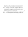
Figure 3.
ADVs mounted on a strongback vane prior to deployment. The heads and bodies are tilted at 15∘
to account for mooring blow-down. NMSS shackles and pear-links connect the strongback to the mooring lines. The strongback is leaning against the anchor stack (railroad wheels). White fair-wrap on the
mooring lines is used to reduce strumming. Plastic ‘zip-ties’ are used to fasten the ADV cables to the
vane. NMSS u-bolts and rubber gaskets fasten the ADV body to the fin. A piece of 1” angle NMSS fastened to the backbone is used to extend the ADV heads approximately 10” foreward of the vane’s leading
edge . . . . . . . . . . . . . . . . . . . . . . . . . . . . . . . . . . . . . . . . . . . . . . . . . . . . . .
5
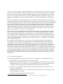
Figure 4.
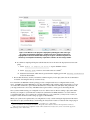
The Nortek Vector program’s deployment planning pane with some typical settings for quantifying turbulence at tidal-energy sites. Required settings are highlighted in red and recommended settings
are in green. The blue box points out the battery consumption and memory requirement estimates for the
settings shown. . . . . . . . . . . . . . . . . . . . . . . . . . . . . . . . . . . . . . . . . . . . . . . . .
7
Figure 5.
An example velocity time-series measured using a TTM at Admiralty Inlet. A) The mean streamwise velocity (ū, blue, ∆t = 5min) is over-layed on the full signal (grey). B) A 5min data window of the
turbulent piece of the streamwise velocity, u′ . The dashed lines indicate one standard deviation. . . . . .
11
Figure 6.
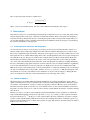
A time-series of turbulence statistics measured from a TTM at Admiralty Head: a) velocity, b)
turbulence intensity, c) turbulent kinetic energy and its components, d) Reynold’s stresses. Shaded regions indicate ebb (red) and flood (blue) periods where U > 0.7. Turbulence intensity is only plotted
during these periods because it is meaningless for small values of U. The mean I over the data record is
10%. . . . . . . . . . . . . . . . . . . . . . . . . . . . . . . . . . . . . . . . . . . . . . . . . . . . . .
15
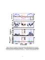
Figure 7.
A histogram of the mean horizontal velocity magnitude. . . . . . . . . . . . . . . . . . . . . . .
16
Figure 8.
A comparison of the shape of spectra at two different sites from ADVs on a rigid tripod (A) and
a TTM (B). The spectra for each velocity component, u, v, w are in blue, green and red, respectively. The
shaded region indicates the ‘inertial subrange’, in which the spectra decay like f −5/3 and all components
have nearly the same amplitude. The dashed line indicates a f −5/3 slope. The difference in amplitude
of the spectra (between A and B) is expected because the turbulence measurements were made at different sites. In each panel the ‘doppler noise’ level arrow points at doppler noise that exceeds the highfrequency turbulence levels. . . . . . . . . . . . . . . . . . . . . . . . . . . . . . . . . . . . . . . . . .
16
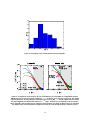
Figure 9.
Spectra of turbulence highlighting motion correction. A) Streamwise velocity, B) cross-stream
velocity, C) vertical velocity. Black lines show the uncorrected spectra, red show spectra of head motion, and blue shows the spectra after motion correction. Green shading highlights locations where motion correction reduced the spectral amplitude. The u and v spectra have sharp peaks at 0.1Hz–and lesser
peaks at higher frequencies–that match the spectrum of ~ueh , indicating motion-contamination. Motion
correction removed the vast majority of the contamination from these spectra, but contamination from
the large peak in the v spectra at 0.1Hz persists. The w spectra is essentially uncontaminated by the
mooring motion. The inertial sub-range is shaded as it was in Figure 8. . . . . . . . . . . . . . . . . . .
17
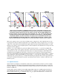
Figure 10. Spatial coherence estimates from TTMs. Vertical coherence estimates (A) are from ADVs on
TTM1 spaced 0.6m apart. Lateral coherence estimates (B) are between neighboring TTMs spaced 50m
apart. Dashed lines in both figures indicate the 95% confidence level above which the coherence estimates are statistically different from 0. . . . . . . . . . . . . . . . . . . . . . . . . . . . . . . . . . . . .
18
vi
Figure 11. The circuit-board and pressure-case end-cap of a Nortek Vector equipped with a Microstrain
IMU. The ADV-body coordinate system (yellow) is depicted on the right. The notch in the end-cap defines the x̂* direction (out of the page), and the ẑ* direction points back along the pressure case axis. A
zoom-in on the Microstrain chip highlights its coordinate system (magenta) relative to the body. . . . . .
25
Figure 12. Coordinate systems of the ADV body and head. A) A strongback with an ADV rests on a block
of wood. Coordinate systems of the ADV head (magenta) and body (yellow) are shown. The x̂head -direction
is known by the black-band around the transducer arm, and the x̂* direction is marked by a notch on the
* . The perend-cap (indiscernible in the image). The cyan arrow indicates the body-to-head vector, ~lhead
head
*
head
*
head
*
spective slightly distorts the fact that x̂
‖ −ẑ , ŷ
‖ −ŷ , and ẑ
‖ −x̂ . B) Coordinate system of
the ADV head as defined in the Nortek Vector manual (Nortek, 2005). . . . . . . . . . . . . . . . . . . . 27
Figure 13. The ‘crop_data.pdf’ figure generated by the adv_example01.py script. The uncropped, uncleaned
data is in red, and the cropped and cleaned data is in blue. . . . . . . . . . . . . . . . . . . . . . . . . . .
34
Figure 14. The ‘motion_vel_spec.pdf’ figure generated by the adv_example01.py script. Spikes in the spectra due to motion contamination (red) are removed by motion correction (blue). . . . . . . . . . . . . . .
35
vii
1
Introduction
Turbulence is a dominant driver of the operational and extreme loads that determine hydro-kinetic turbine (HKT)
lifetime. Device simulation tools, such as HydroFAST and Tidal Bladed have been developed to estimate HKT
power performance and lifetimes based on device mechanical-electrical models and realistic inflow conditions.
These tools help to accelerate the HKT industry by, 1) helping device designers predict failure modes in preliminary designs, and 2) providing site developers and financial institutions with estimates of the cost of energy for a
particular device.
Device designers typically have all of the information necessary for producing device models for these simulations,
but often lack adequate knowledge of turbulent inflow conditions to produce accurate power-performance and lifetime estimates. This gap arises from the difficulty and high-cost of making turbulent inflow measurements that are
relevant to HKTs. Furthermore, the method for measuring turbulent inflow must be suited to the energetic sites
where HKTs will be deployed. This work aims to fill this gap by detailing a relatively low-cost and robust methodology for measuring the turbulent inflow statistics relevant to HKTs.
The question, “What turbulent statistics determine turbine device performance and fatigue loads?” motivates an active area of research in both the wind-turbine and HKT industries. While no single statistic–or group of them–has
been identified that fully predicts fatigue loads, there is broad agreement that mean-shear, Reynold’s stresses, the turbulence spectrum1 , and spatial coherence all contribute significantly to fatigues loads. If turbulence is conceptualized
as a mixture of eddies of different sizes, orientations and rotation speeds (Figure 1) the importance of these statistics
can be understood as follows:
∙ Mean shear can impart a torque on the rotor shaft and induce variable loads on the blades as they rotate
through the spatially non-uniform mean flow.
∙ The Reynold’s stresses (u′ v′ , u′ w′ and v′ w′ ) indicate the orientation of the eddies in the flow. Eddies of different orientations may impart forces on different components of the turbine differently. For example an eddy
aligned with the rotor (v′ w′ in Figure 1) will impart a large torque on the rotor that eddies of other orientations
would not.
∙ The turbulence spectra quantifies the energy of eddies of different frequencies (from which length scales δ can
be estimated). For example, an eddy with δ similar to the blade cord (lcord ) is likely to impart larger fatigue
loads on the blade than a smaller or larger eddy with the same energy. Likewise, an eddy the same size as the
rotor will impart a larger load on the rotor than a much smaller eddy. Quantifying the energy in these eddies is
therefore important to accurately estimating the loads they induce.
∙ Spatial coherence quantifies the correlation of the turbulence in space, i.e. the length, L, of the eddies. It is
important because longer eddies are likely to impart larger forces than shorter ones and longer eddies are likely
to be anisotropic such that L > δ .
The first two of these, mean shear and Reynold’s stresses, can be measured using acoustic Doppler profilers (ADPs)
(Stacey et al., 1999; Thomson et al., 2012). The Reynold’s stresses, turbulence spectra, and spatial coherence can
be measured using acoustic Doppler velocimeters (ADVs). This situation requires that detailed turbulence measurements at tidal energy sites requires measurements using both ADPs and ADVs. The deployment of ADPs on the
seafloor for this purpose is well described and commonly performed by engineers, scientists and ocean professionals
around the world.
While ADVs have the accuracy to measure detailed statistics of turbulence, they must be positioned at a point in the
flow that is relevant to HKTs, i.e. at hub-heights of 10m or more. While it is possible to do this using rigid towers,
such an approach is technically challenging and expensive to implement at tidal energy sites (where currents often
exceed 3 m/s). To reduce the cost of hub-height turbulence measurements this document details a methodology for
making turbulence measurements from moorings. This approach is made possible by the recent integration of inertial
1 Turbulent
energy and turbulence intensity can be computed from this.
1
Mean Velocity
Turbulence
L
Instantaneous
Flow Field
Mean Flow Profile
Figure 1. Diagram of turbulent inflow to a MHKT. The mean-flow profile is indicated in blue,
and turbulent eddies of different sizes (δ ), lengths (L), and orientations are indicated in red.
motion sensors (IMUs) into ADVs, which measuring ADV (mooring) motion so that it can be removed from the
measured velocity.
Section 2 describes hardware details of the mooring used and ADV configuration details specific to moored measurements. Section 3 details the processing steps for transforming moored ADV measurements into earth-frame velocity
signals and computing turbulence statistics from those measurements. Section 4 describes turbulence analysis methods that are useful to the HKT industry and defines the applicability and limitations of the results. The reader is also
encouraged to download and install the Doppler Oceanography Library for pYthoN software package (DOLfYN
lkilcher.github.io/dolfyn/), which provides example instrument configuration files and functions for performing the
data processing and analysis steps described herein.
2
Measuring turbulence
Acoustic Doppler velocimeters (ADVs) are capable of high accuracy, precision (< 1%), and sample rates (up to
64hz). These characteristics make them the preferred tool for measuring the spectrum and spatial coherence of
turbulence at tidal-energy sites. However, they measure the water velocity within a few inches of the sensor-head.
Therefore, in order to resolve turbulence that is relevant to MHKTs, these instruments must be positioned near the
hub-height of the MHKTs that will be deployed at that location. This section describes the mooring used, and the
details the configuration of instrumentation for measuring turbulence from a moored platform.
2.1
Mooring Hardware
The ‘Tidal Turbulence Mooring’ (TTM) mooring is a simple, compliant, sub-surface mooring (Thomson et al.,
2013). Its primary components are a clump-weight style anchor, an acoustically triggered release for mooring recovery, mooring lines, a ‘strongback’ vane at turbine hub-height that orients the ADVs into the flow (i.e., passive
2
yaw), and a buoy that holds the mooring lines taught (Figure 2). The clump weight is composed of 3 railroad wheels
stacked on a central steel cylinder. A steel flange welded securely to the base of the cylinder supports the weight of
the wheels. The total wet-weight of the anchor is 2500lbs. Galvanized 1/2” anchor chains and a 5/8” steel shackle
connect the top of the anchor-stack to the acoustic release (manufacturer: ORE, now EdgeTech). At the top of the
acoustic release a high-tension swivel allows the mooring line to rotate without imparting torque on the hardware
below.
The buoy for the TTM is a 37” diameter spherical steel buoy (manufacturer: McClane) that is pressure-rated for the
depths to which it will be deployed. Another high-tension swivel between the buoy and mooring line allows the buoy
to spin without imparting large torques on the mooring line. Half-inch Amsteel line (e.g. http://www.amsteelblue.com/)
is used to connect the strongback-vane to the buoy and acoustic release (using 5/8” shackles). Amsteel line has a
high strength-to-weight ratio, low stretch, and low torque. The half-inch line used here has a breaking strength of
30,600lbs, much larger than the dry-weight of the mooring (<3,500lbs). If modifications are made to the mooring
design, to avoid catastrophic damage, be sure that the mooring line can safely support the weight of the mooring
during recovery (a safety factor of at least 5× is recommended).
The ‘blow-down’ angle of the TTM was simulated using University of Victoria’s Mooring Design and Dynamics
software. The observed blow-down angle of 20∘ at 2 m/s agreed well with the predictions (Thomson et al., 2012).
This mooring design has been safely deployed in currents up to 3 m/s without exceeding a maximum advisable
blow-down angle of 40∘ . If significant modifications are made to this mooring design (such as changes in mooringlength, deployment depth or other modifications to major hardware components), or if operating in much stronger
currents, the new design should be re-simulated using a mooring simulation tool to determine blow-down angle as
well as tension and drag forces.
The strongback-vane was designed to be a robust and low-cost component that effectively holds an ADV head
(or two) upstream of the mooring line and holds the ADV body nearby and rigidly fixed-to its head (Figure 3).
All components of the strongback-vane, including shackles, are constructed from non-magnetic materials (highdensity plastics and non-magnetic stainless steel) so that the IMU-compass can accurately resolve the undistorted
magnetic field of the earth (i.e. measure North). If magnetic materials must be used in the vicinity (within ≈ 2m) of
the ADV body the IMU compass should be recalibrated in the presence of those magnetic materials and in the exact
orientation as they will be deployed (Nortek, 2005). At its leading edge flat-stock NMSS sandwiches the plastic-fin
to form the strongback ‘backbone’. 3/4” holes are drilled through the top and bottom of the backbone so that NonMagnetic Stainless Steel (NMSS) shackles can connect the strongback to the mooring lines (Figures 3).The ADV
heads and bodies are tilted 15∘ from the vertical-axis of the strongback to account for the ‘mooring blow-down’ of
10-20∘ at 2 m/s.
2.2
Instrument configuration
When preparing instrumentation for deployment always follow the manufacturers recommendations. Be sure to:
1. Perform bench tests to confirm the instrument is operating correctly2 .
2. Install batteries with sufficient capacity for the deployment. Manufacturers configuration software can aid in
determining battery life. It is recommended to use non-rechargeable batteries because rechargeable batteries
can degrade overtime (resulting in early instrument shut-down and an incomplete data record).
3. Seal pressure-cases carefully and install dessicant (moisture-absorbing) packs to reduce the risk of waterdamage to electrical hardware.
4. Synchronize instrument clocks to a single computer clock that has been recently syncronized to internet time
via Network Time Protocol (NTP).
5. Configure the instrument appropriately for the deployment.
2 Perform
bench-tests several weeks prior to the deployment to allow time to replace faulty components if necessary.
3
Figure 2. Schematic diagram of the tidal turbulence mooring (TTM).
In order to produce high-fidelity spectra and spatial coherence estimates from moored ADV measurements, motionsensor measurements must be tightly synchronized with ADV velocity measurements. Currently Nortek’s VectorTM is
the only instrument that can be purchased ‘off the shelf’ with a tightly synchronized inertial motion sensor (IMU).
These instruments were used for the TTM test deployments.
2.2.1
Record position and orientation of the ADV head
For deployments involving cable-head IMU-ADVs, it is critical to record the position and orientation of the ADV
head relative to the ADV body (pressure case). Details of the definitions of these coordinate systems can be found
in appendix A. The variables should be measured as accurately as possible, as errors will propagate through motioncorrection calculations and lead to errors in the motion-corrected velocity measurements. As a rule of thumb: the
*
vector ~lhead
should be measured to within a few mm. The orientation matrix of the ADV-head, H, should be measured to within ≈ 2%, (≈ 2 Euler-angle degrees).
2.2.2
Software configuration
At least as important as recording the orientation of the ADV head relative to the ADV body is configuring the ADV
to record the correct data channels for performing motion correction. Three primary data channels are needed to
perform motion correction.
1. The linear acceleration vector, ~a, is integrated to obtain an estimate of the translational-velocity of the ADV
body and head.
~ , is used to estimate the velocity of the head that is due to rotation of the
2. The angular rotation rate vector, ω
ADV about the IMU.
4
Figure 3. ADVs mounted on a strongback vane prior to deployment. The heads and bodies are tilted at
15∘ to account for mooring blow-down. NMSS shackles and pear-links connect the strongback to the
mooring lines. The strongback is leaning against the anchor stack (railroad wheels). White fair-wrap on
the mooring lines is used to reduce strumming. Plastic ‘zip-ties’ are used to fasten the ADV cables to the
vane. NMSS u-bolts and rubber gaskets fasten the ADV body to the fin. A piece of 1” angle NMSS fastened
to the backbone is used to extend the ADV heads approximately 10” foreward of the vane’s leading edge
5
3. The (body) orientation matrix, R, provides the orientation of the ADV body relative to the earth. It is used
(with H) to estimate the earth-frame orientation of the ADV-head, and thus the velocity vector in the earthframe. It is also used to remove gravity from the linear acceleration measurement (see section 3).
The Nortek Vector can be purchased with a Microstrain GDM-GX3-25 ‘miniature attitude heading reference system’
(MicroStrain). The 3DM-GX3-25 can output all three of these channels. Sampled and stored in realtime by the same
controller, the Vector velocity measurements and 3DM-GX3-25 motion and orientation measurements are tightly
synchronized (to within 10−2 sec), allowing for high-fidelity motion-correction in post-processing. New versions of
the Nortek software (bundled with a new Vector) allow the user to select which datastreams from the 3DM-GX3-25
are stored in the Vector output data file.
To set a Vector to record the correct data, open the “Vector” program and go to Deployment » Planning
» Use Existing . For most situations you should only need to use the ‘Standard’ tab. The following settings
are required to be able to perform motion correction (Figure 4):
1. Check the box to the left of IMU: .
This tells the Vector to use and record information from the IMU.
2. Select Accl AngR Mag xF from the drop-menu to the right of IMU: .
This tells the Vector to record the acceleration (Accl), Angular Rate (AngR), Magnetometer (Mag), and Orientation Matrix (xF) signals3 .
3. For the Coordinate system select XYZ .
This instructs the Vector to record data in the ADV-head coordinate system.
For most measurements of turbulence at tidal energy sites, the following recommendations are also likely to be
appropriate:
4. Set the Sampling Rate to 16 Hz .
In most tidal environments lower sampling frequencies will not resolve all of the turbulence scales. Higher
sampling frequencies are typically dominated by instrument noise.
5. Set Geography to Open ocean .
This instructs the ADV to operate in ‘high’ power mode which increases data quality. Consider upgrading
batteries (use 2 Lithium batteries if necessary), or using burst sampling before using lower power ‘Surf zone’
or ‘River’ setting. See the instrument manual for further details.
6. Set the Nominal velocity range to +/- 4 m/s .
Tidal velocities at most tidal energy sites will be in this range. Use the higher range of +/- 7 m/s if you
have reason to believe the velocities will be larger than 4 m/s (at the expense of some data quality).
7. Set Speed of Sound to Measured .
The Nortek Vector uses a temperature sensor and a fixed Salinity value to calculate an estimate of the
speed of sound (which is important to the velocity measurements). If the salinity of your site is not known
consider measuring it.
8. Modify the burst interval settings to maximize data return. If you are going to the effort of putting this instrument in the water, it is valuable to capture as much turbulence data as possible. Once the above settings have
been set, follow these guidelines to maximize data recovery:
A. Use Continuous sampling if possible. Consider purchasing additional batteries. With the settings
recommended above, 2 Lithium batteries will last 11 days, and 2 Alkaline batteries will last 3.3 days.
3 The
magnetometer signal is not needed for motion correction, but the other three signals are. Note that this is the only option that provides
the orientation matrix, which is required for motion correction.
6
Figure 4. The Nortek Vector program’s deployment planning pane with some typical settings for quantifying turbulence at tidal-energy sites. Required settings are
highlighted in red and recommended settings are in green. The blue box points out
the battery consumption and memory requirement estimates for the settings shown.
B. If continuous sampling will deplete available batteries before the end of the deployment use burst sampling:
i. Set the Number of samples per burst to capture 10-20min of data4 .
ii. Set the Battery pack selection to the batteries that are available5 .
iii. Adjust the burst interval–which must be greater than the sampling period–until Battery utilization
is between 90 and 100%.
9. Be sure that the memory card in your ADV has sufficient capacity for the deployment. See the documentation
for details on clearing the memory card if necessary.
For convenience, the DOLfYN software package provides a sample Nortek Vector configuration file, Nortek_Vector_with_IMU.dep (in the <DOLfYN-root>/config_files/ADV/ folder) with the settings described above. To use
one of these files download it, open it with the Nortek Vector software then view and adjust other parameters to fit
your deployment needs as necessary6 . The IMU-related options will be correctly pre-set when using this file.
Once you have finished setting your configuration save it to disk for later use. Before starting a deployment, make
sure that your computer’s system time has recently been synchronized via NTP, and that it is set to the timezone
you wish the ADV data to be recorded in. If you make changes to your system time, you may need to restart your
computer to make sure the new time settings propagate to the instrument.
When your system clock is updated and your configuration is ready, consider starting the deployment. If the instrument will not be deployed immediately consider using the ‘delayed start’ feature to reduce the risk of deploying an
4 At
16Hz a 10min burst will have (10 min) · (60 sec/min) · (16 samples/sec) = 9616 samples.
is not recommend to use recharged Li-Ion batteries. The capacity of these batteries can be less than expected after several uses.
6 Older versions of Nortek’s Vector configuration software will not load this file correctly, be sure you have a version that supports the
Microstrain chip (version 136b6 or later).
5 It
7
instrument that does not collect data. Take care to make sure that the start times agree with the actual physical deployment times in your cruise plan (set the instruments to start before you deploy them so that you can listen to the
transmit transducer to confirm that it is operating). It is also important to synchronize your computer’s clock prior to
powering-down so that the clock-drift estimate provided by the Nortek Vector software is as accurate as possible.
2.3
Deployment Planning
Safe, efficient and accurate deployment of scientific equipment in the oceanic environment is a science of its own.
Carefully considered planning is critical to deployment safety and success. HKT sites are generally locations of
strong currents that add to the difficulty and complexity of deploying scientific equipment. It is highly recommended
that deployment in these environments be led by experienced professionals in the field. At the very least, enlist such
professionals to advise your planning and deployment process.
A well-written ‘research cruise plan’ should include the following information:
∙ Scientific objectives,
∙ A detailed schedule of all activities needed to accomplish objectives,
∙ Noteworthy environmental conditions at the deployment site (e.g. tidal amplitude, current amplitude, probable
weather conditions, daylight hours, etc.)
∙ Schematic diagrams of hardware that will be deployed,
∙ A list of all personnel involved in the deployment,
∙ Maps of deployment locations that include notable bathymetric features (e.g. sub-surface ridges or canyons)
and human infrastructure hazards (e.g. buoys or other equipment).
∙ A risk assessment and risk mitigation plan.
The schedule is one of the most important parts of the cruise plan. It should include personnel arrival/departure
times, ship arrival/departure times, ship-loading and ship-preparation periods, transit periods between port and deployment locations, and target deployment times. Deployment and recovery should be conducted during slack tides
to minimize risks associated with the strong currents present during ebb and flood. When preparing the schedule take
care to realistically assess the time needed for each piece of the cruise; when in doubt allow ‘contingency’ time for
each period. The instruments should be deployed for at least two full-tidal cycles, and ideally up-to 6 or more tidal
cycles. Site characterization measurements for power availability should be much longer (see Polagye and Thomson,
2013).
3
Data processing
Data processing involves reading raw data from an instrument and converting it to a form that can be readily analyzed, in general it includes cleaning (removing) ‘bad’ data points, converting to consistent scientific units, producing high- or mid-level variables from the raw data and averaging.
Often times during the analysis stage unexpected or unrealistic results will indicate errors in the data. When this
happens it is necessary to cycle back through data processing steps to inspect raw data and locate the source of the
error and clean (remove) bad data. The difference between good and bad data is generally stark, but when it is not
and no viable justification can be made for removing the unexpected data one should err on the side of keeping the
data and, if necessary, treating it as a special case.
Fortunately, the reliability of velocity measurements from instruments such as ADVs and ADPs is high, the uncertainties well understood and methods for cleaning data are well defined. Instruments generally provide estimates of
various sources of uncertainty and other errors as part of their output data streams (e.g. ‘error velocity’ and beam
‘correlation’) that aid in cleaning data.
8
As the scientific community has become familiar with these measurements, well defined and justified methods for
cleaning data have been developed and shown to be effective (e.g. Goring and Nikora, 2002). This means that it is
now possible to generate meaningful and reliable statistics with minimal user input and inspection. The DOLfYN
software package includes tools and scripts for processing and analyzing turbulence measurements made following
the procedures in this document.
There are four major steps to processing moored ADV data:
1. read the raw data from the ADV data file and crop it to the period of interest,
2. remove ADV head-motion from measured velocity and rotate data into a useful coordinate system,
3. clean erroneous points from the ADV data record,
4. compute turbulence statistics and averages.
It is common practice to save the results of these steps some or all of these steps so that later analysis does not
require reprocessing (which sometimes requires significant CPU-time). The DOLfYN software package has tools for
performing each of these steps, and for saving data along the way. See appendix C for an example processing script.
3.1
Reading data
ADVs typically record data internally in a compact vendor-defined binary format. The vendor will generally publish
the details of the data format (e.g. Røstad, 2011), and also release software tools for viewing this data and/or writing it to other common data formats (e.g. white space-, comma- tab-delimited formats, MatlabTM format, or other
increasingly common standards such as HDF5).
Nortek provides software tools for converting raw/binary ‘.vec’ files to MatlabTM format (see http://www.nortekas.com/en/support/software), and the DOLfYN software package is capable of reading these files directly into
Python NumPy arrays (appendix C, line 40). A dataset will also generally need to be ‘cropped’ to the period of
interest (e.g. when the instrument was in place on the seafloor, Figure 13).
3.2
Motion Correction
Raw turbulence measurements from moored ADVs will be contaminated by mooring motion. When IMU measurements are tightly synchronized with standard ADV velocity estimates, the IMU measurements can be used to
reduce this contamination. This involves removing the measured velocity induced by ADV head-motion, ~ueh , from
the measured velocity, ~uem , to estimate the ‘motion corrected’ velocity in the earth frame,
~ue (t) = ~uem (t) −~ueh (t)
.
(1)
Here superscript ‘e’s denotes the earth coordinate system.
We now break ~ueh into two parts, ~ueh = ~uea +~ueω . The first is an estimate of the linear motion of the ADV,
~uea (t) = −
Z
{~ae (t)}HP( fa ) dt
.
(2)
Here, ~ae (t) is the IMU-measured acceleration signal rotated into the earth frame7 , and {}HP( fa ) denotes an appropriate high pass filter of frequency fa . The acceleration must be high-pass filtered in this way to remove the influence
of gravity and that of low-frequency bias (bias drift) that is inherent to IMU acceleration measurements (for further
details see appendix B and Egeland (2014)).
7 i.e. ~
ae (t) = RT (t) ·~a* (t),
see appendix A for details.
9
The second component if ~ueh is due to rotational motion of the ADV-head about the IMU,
~ * (t) × ~`*
~ueω (t) = −RT (t) · ω
.
(3)
*
* is the vector from the IMU to the ADV head, × indi~ * is the IMU-measured rotation-rate, ~`* = ~lhead
Here ω
−~limu
cates a cross-product and superscript *s denotes a quantity in the ‘ADV body’ coordinate system. This coordinate
system is used explicitly here to emphasize that ~`* is constant in time. Matrix multiplication (denoted by ‘·’) with
the inverse ADV body orientation matrix, RT (t), is used to rotate the ‘body-frame rotation induced velocity’ into
the earth frame. For details on these coordinate systems and the definition of the orientation matrix see appendix A.
The minus signs in equations (2) and (3) are correct because the measured velocity induced by head motion is in the
opposite direction of the head motion itself.
All of the steps can be performed using DOLfYN’s adv.io.rotate.CorrectMotion class. To do this, you will need to
*
specify H and ~lhead
as ‘properties’ of your raw (cleaned) adv data object, and select a value for fa (e.g. lines 18,
23, 34, 108-111 of appendix C). For those unfamiliar with Python, the ‘motcorrect_vectory.py’ script bundled with
DOLfYN provides a command-line interface for performing this motion correction and saves the motion-corrected
*
data in MatlabTM format. In that case H and ~lhead
are specified in an input ‘orient’ file, and fa can be specified as a
command-line option.
3.2.1
Select a local coordinate system
Prior to performing any averaging and computing other statistics it is often useful to rotate the measurements into a
locally meaningful coordinate system. For the purposes of quantifying turbulence at HKT sites it is common practice
to rotate the data into a coordinate system in which u is the ‘streamwise’ velocity, v is the ‘cross-stream’ velocity
and w is in the ‘up’ direction. For details on selecting, estimating and transforming-into such a coordinate system see
appendix A.2.
3.3
Cleaning data
Data ‘cleaning’ is a two-step process of 1) identifying erroneous (bad) points in an otherwise good dataset and 2)
replacing them with either a) reasonable estimates of the values at those points, or b) ‘error values’ (e.g. NaN = ‘nota-number’) which explicitly indicate the points are invalid. Several methods exist for identifying bad data. These
include:
1. Search the data for manufacturer-defined ‘error values’ (if the manufacturer defines these8 ).
2. Search for values outside a reasonable range. For example, tidal velocities are typically less than 4m/s; therefore a velocity measurement greater than 5m/s is probably bad. Histograms can be useful for identifying the
reasonable velocity range. The distribution of velocity measurements will often be approximately Gaussian;
values well-beyond the tails of the distribution (>3 standard deviations) can probably be identified as bad.
3. Utilize diagnostic data from the instrument to identify bad data. For example, low values of ‘correlation’–the
similarity of the send and receive acoustic pulses–can sometimes indicate bad data.
4. Apply ‘spike detection’ algorithms to the velocity signal. While turbulence is, by definition, unsteady and
chaotic it is not discontinuous. Large and sharp spikes in the velocity signal are almost always bad.
Modern ADVs often produce data of sufficiently high quality that only a relatively small number of spike-type bad
data points are present in the raw data (after cropping). In these cases spike-detection is usually sufficient to identify
bad points. The recommended spike-identification method is documented in Goring and Nikora (2002) and Wahl
(2003), and implemented in DOLfYN’s adv.clean.GN2002 function.
8 The
velocity data in Nortek Vector (.vec) files do not contain an error value.
10
ū [ms−1 ]
u0 [ms−1 ]
3
2
1
0
1
2
3
0.6
0.4
0.2
0.0
0.2
0.4
0.6
0
(a)
00:00
04:00
08:00
Time [June 16, 2014]
12:00
(b)
50
100 150 200
Time [seconds]
250
300
Figure 5. An example velocity time-series measured using a TTM at Admiralty Inlet. A) The mean
stream-wise velocity (ū, blue, ∆t = 5min) is over-layed on the full signal (grey). B) A 5min data window
of the turbulent piece of the streamwise velocity, u′ . The dashed lines indicate one standard deviation.
After points have been identified as bad they will need to be replaced. For cases of a small number of sparsely
distributed bad data points they can be replaced with interpolated values (DOLfYN’s adv.clean.GN2002 function
uses a least-squares cubic-polynomial) without introducing significant interpolation-related bias. This approach
produces a dataset that can be further processed without the headache of dealing with NaN values.
If, on the other hand, there are segments of data with large fractions of bad points (>10-20%) interpolation may
introduce significant bias to a myriad of statistics of the data. In these cases it is best to crop-out the bad segment
(perhaps creating two distinct data sets that can be rejoined later), or to assign NaN values to the bad points. In
general, the choice between these options will depend on the objectives of the analysis or the preference of the investigator. For the purposes of this document, in which spectral analysis is a primary result, assigning NaN values will
make spectral analysis difficult to the point that it is best to simply split the data record to remove the bad segments
and plan to recombine in later stages of processing.
3.4
Turbulence metrics and averaging
Having cleaned the raw data and computed an estimate of the velocity vector in a useful coordinate system, ~u, one
can finally begin estimating the turbulence statistics and average (mean) flow properties the measurements were designed to capture. For each component of velocity, ~u = (u, v, w), turbulence is defined by separating the instantaneous
11
velocity (e.g. u) into ‘average’ (ū) and ‘turbulent’ (u′ ) pieces9 ,
u = ū + u′
.
(4)
Where the over-bar denotes a ‘suitable average’, over a period ∆t, such that u′ = 0. For HKTs, it is useful to choose
∆t such that ū is the flow which the turbine is designed to efficiently convert into useful energy, while the turbulence
is what contributes to fatigue loads that decrease device lifetime. That is, ∆t should be somewhat longer than a
typical HKT ramp-up time (tens of seconds to a minute or two). Defined this way a turbine can be considered to be
in a ‘steady operational state’ so long as changes in ū are small compared to ū itself. Turbulent velocity fluctuations
can then be treated as disturbances to a HKT’s ‘steady operation’.
A time scale ∆t must be chosen such that the tidal flow has stationary statistics (i.e., stable mean and variance) for
that duration of tide. If ∆t is too long, the tidal variation itself will contaminate the results. The wind energy industry
uses ∆t = 10min (Commission, 2005). This is appropriate for large modern wind turbines (with long ramp-up times),
but the smaller size of current HKTs suggests that they may respond faster and therefore that a smaller ∆t might be
appropriate (Gunawan et al., 2014). On the other hand, if turbulence is to be treated as the primary driver of device
fatigue loads one should be careful not to implicitly neglect energetic low-frequency turbulence by selecting ∆t to be
too short.
With these considerations in mind, and until further work provides details on the relationship between turbulent
inflow and HKT loads, this document recommends using ∆t = 2-10 minutes. The exact choice of ∆t–within this
range–is unlikely to alter the results significantly, and should be adjusted depending on the goals of the analysis. For
example, when fitting theoretical spectra to observations for the purpose of input to stochastic flow simulation tools
such as TurbSim (Jonkman, 2009), it is desirable to include lower frequencies in the fit, and therefore it is reasonable
to use a longer ∆t (5-10min).
With ∆t chosen the ADV data record is broken into segments in which turbulence statistics are computed. In this way
the time-series of instantaneous velocity, ~u (at the instrument sample rate, e.g. 16Hz), is converted to a time-series
of turbulence statistics (with time-step ∆t, Figure 5). It is recommended to save your data at this level to allow quick
and easy access during analysis.
The remainder of this section defines several turbulence variables that are commonly used in the HKT industry and
can be computed from moored ADV measurements. Furthermore, DOLfYN’s adv.io.turbulence.TurbBinner provides
a two line interface for performing averaging and computing all of these statistics (e.g. lines 124-125 in appendix C).
3.4.1
Turbulence intensity
Turbulence intensity is used throughout the wind industry, and other engineering fields as a zeroth-order metric for
quantifying
turbulence. It is defined as the ratio of the standard deviation of horizontal velocity magnitude (U =
√
u2 + v2 ) to its mean,
I=
std(U)
Ū
.
Turbulence intensity is often quoted in units of percent (i.e. 100 · I). It is useful because it is easy to understand
and–in many observations of atmospheric and oceanic turbulence–is relatively constant for Ū ≫ 0. On the other
hand, I has often been criticized for being too simple (in particular that it only includes information about horizontal
velocity) such that it does not provide enough information about the turbulence for various applications.
3.4.2
Turbulent kinetic energy
9 Some
discussions include a ‘wave velocity’ but, for simplicity, it is not included here at this time.
12
Turbulent kinetic energy (tke) quantifies the total energy contained in turbulence,
Etke = u′ u′ + v′ v′ + w′ w′
.
Like I, Etke , is useful because it is relatively simple. As a scalar quantity that includes all turbulence components,
it has been studied at length by turbulence scientists and it has a well defined ‘budget’ equation that is the basis of
turbulence theory. For some purposes it may be useful to investigate each component of
√Etke individually. Lastly,
it has sometimes been suggested that a turbulence intensity based on tke, that is Itke = Etke /Ū, would be more
meaningful to engineering applications but this approach has not gained wide acceptance.
3.4.3
Reynold’s stresses
Reynold’s stresses are correlations between velocity components and are fundamentally important to turbulent flow
fields. Unlike Etke , Reynold’s stresses appear in the mean-flow equation explicitly as terms that transport (move)
momentum from high velocity to low velocity regions. Because of how they appear in the mean-flow equation,
Reynold’s stresses are typically treated as three distinct components, u′ v′ , u′ w′ , and v′ w′ 10 . Several recent studies
have found evidence that they are correlated with increased wind-turbine fatigue-loads (e.g. Kelley et al., 2002,
2005), which has begun to elevate their importance in the wind-energy field.
3.4.4
Turbulence auto-spectra
Turbulence velocity auto-spectra (hereafter, simply ‘spectra’) are estimates of the distribution of turbulent energy
as a function of frequency. That is, a spectrum quantifies the amount of energy in the velocity at a range of timescales. Furthermore, since time-scales can be converted into length scales using Taylor’s frozen flow hypothesis
(i.e. li = ū/ fi ), spectra quantify the distribution of turbulent energy at different length-scales. When considering
turbulence to be a complex interaction of eddies from very small to very large scales, the spectrum quantifies the
energy (rotation speed) of the eddies as a function of their size (δ , Figure 1).
HKTs respond to different scales of velocity fluctuations (different eddy sizes) differently. HKT simulation tools
(such as Tidal Bladed, and HydroFAST11 ) are capable of estimating the loads induced by these fluctuations, but the
critical information of how energetic those fluctuations are, must be provided as input to these tools. Fortunately,
spectra provide exactly this information: the distribution of energy as a function of eddy size.
Spectra are estimated from Fourier transforms (Fast Fourier Transforms) of the turbulent velocity,
S{u}( f ) = |F (u)|2
.
In this work FFTs (denoted by F ()) are computed by removing a linear trend (fit) fromRu12 and applying hanning
windows to reduce spectral reddening (Priestley, 1981). Spectra are normalized so that S{u}( f )d f = u′ u′ .
3.4.5
Spatial coherence
Spatial coherence is an estimate of the correlation of velocity components, over spatial distances, as a function
of frequency. That is, where spectra indicate the energy in eddies as a function of their size (δ ), coherence is an
estimator of their ‘length’ (L). For 3D isotropic turbulence, these length scales should be similar. For the largest
eddies, which are expected to be depth-limited and thus 2D anisotropic, it is likely that L will greatly exceed δ .
Knowledge of the ‘length’ of these large eddies is important to HKT design because they are the most energetic and
if their dimensions match that of HKT components they are likely to have a larger impact on the HKT.
10 In many formalisms of turbulence the Reynold’s stresses are components of off-diagonal elements of the Reynold’s stress tensor. In these
arenas the diagonal elements of that tensor are the components of Etke .
11 Based on the NWTC’s FAST wind-turbine simulation tool
12 Note that removing a linear trend means that F (u) = F (u’).
13
The u-component spatial coherence is estimated as13 ,
D
E
F (ui )F (u j )2
Γi j {u}( f ) =
⟨Si {u}⟩ S j {u}
.
Where ⟨⟩ denotes an ensemble average, and i and j denote different measurement points in space.
4
Data analysis
Data analysis is the process of synthesizing useful knowledge or information from a set of data. The details of data
analysis depend entirely on the goals of the analysis and the data available. That is, what question is attempting to
be answered and how suitable is the dataset to answering that question? This section presents example analyses of
moored-ADV data that provides potentially useful information for HKT site and device developers, and discussing
the accuracy and limitations of the approach.
4.1
Initial inspection: time-series and histograms
As a first step in most analysis of velocity data, it is useful to plot the velocity and other turbulence statistics as a
function of time. In the example data in Figure 6 the tidal currents reach 2m/s. During this period, at this location,
the floods are significantly larger than the ebb. The mean velocity appears to be a reasonable estimate–there is a clear
tidal signal, there are no sudden dramatic jumps in the values, and the magnitude of the velocity agrees with previous
measurements at this site–this gives us confidence that our methods have produced a reliable dataset (Figure 6A).
The instantaneous turbulence intensity has an average of 10%, but approaches 20% in some 5-min periods (6B).
As is often observed in turbulent flows throughout the oceans and atmosphere the turbulence is highly intermittent,
that is it is dominated by large spikes and periods of relative calm (6C). Note also that the turbulence is significantly
lower for the small ebb than it is for the two (larger) floods. The Reynold’s stresses show a similar pattern (6D).
HKT site-developers often use histograms of velocity measurements to estimate the available power at a tidal energy
site. The record in Figure 6 isn’t long enough to estimate annual energy production, or AEP, but a histogram of the
measurements does provide some indication of the distribution of velocity at the site (Figure 7). During this time
period, for example, more than 30% of the measurements had a Ū in the range of 0.8-1.2m/s.
4.2
Turbulence Spectra
The primary purpose for making ADV measurements at HKT sites is to measure the turbulence spectra. That is,
ADVs resolve the inflow at a level of detail that cannot be measured with profiling instruments. Turbulence spectra
are estimates of the distribution of energy as a function of frequency (eddy size). Because spectra reveal detailed
information about the signal (velocity) they also reveal detailed sources of error in the measurement. It is therefore
important to be aware of these errors so that one can be careful to exclude them from estimates of statistics meaningful to the flow.
Kolmogorov’s theory of locally isotropic turbulence predicted that turbulence spectra would have an ‘inertial subrange’ in which the amplitude of the spectral components (i.e. S{u}, S{v} and S{w}) will be equal, and in which
the spectra will decay as k−5/3 (Kolmogorov, 1941). This prediction has been confirmed by observation so ubiquitously in oceanic and atmospheric turbulence that it has become a defining characteristic of turbulence spectra (e.g.
Figure 8A, data from Thomson et al. (2012)). Based on this we expect that deviations from this behavior are likely to
indicate some source of error.
13 Equivalent
expressions apply for the v and w components.
14
Velocity [m/s]
I
[m2 /s2 ]
Turbulent Energy
[m2 /s2 ]
Reynold's stresses
2
1
0
1
2
0.20
0.15
0.10
0.05 ­ ®
I all =0.10
0.00
0.25
0.20
0.15
0.10
0.05
0.00
0.05
0.04
0.03
0.02
0.01
0.00
0.01
0.02
00:00
(a)
ū
v̄
w̄
(b)
u00u00
v v0 0
ww
Etke
(c)
u00v00
u0 w0
vw
(d)
04:00
08:00
Time [June 16 2014]
12:00
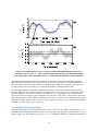
Figure 6. A time-series of turbulence statistics measured from a TTM at Admiralty Head: a) velocity, b)
turbulence intensity, c) turbulent kinetic energy and its components, d) Reynold’s stresses. Shaded regions indicate ebb (red) and flood (blue) periods where U > 0.7. Turbulence intensity is only plotted during
these periods because it is meaningless for small values of U. The mean I over the data record is 10%.
15
35
30
% of data
25
20
15
10
5
0
0.0
0.5
1.0
1.5
Ū [m/s]
2.0
2.5
3.0
Figure 7. A histogram of the mean horizontal velocity magnitude.
Fixed ADV
100
Inertial
Subrange
10-1
[(m2 /s2 )/hz]
Moored ADV
Persistent
motion
contamination
(A)
Successful
motion
correction
10-2
10-3
10
-4
10-3
(B)
Inertial
Subrange
© ª
S©uª
S©v ª
Sw
10-2
Doppler Noise
Doppler Noise
10-1
f [hz]
100
101
10-3
10-2
10-1
f [hz]
100
101
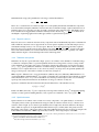
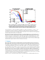
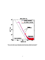
Figure 8. A comparison of the shape of spectra at two different sites from ADVs on a rigid tripod (A) and a
TTM (B). The spectra for each velocity component, u, v, w are in blue, green and red, respectively. The shaded
region indicates the ‘inertial subrange’, in which the spectra decay like f −5/3 and all components have nearly
the same amplitude. The dashed line indicates a f −5/3 slope. The difference in amplitude of the spectra (between A and B) is expected because the turbulence measurements were made at different sites. In each panel
the ‘doppler noise’ level arrow points at doppler noise that exceeds the high-frequency turbulence levels.
16
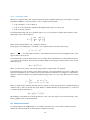
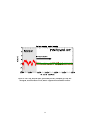
Figure 9. Spectra of turbulence highlighting motion correction. A) Streamwise velocity, B) crossstream velocity, C) vertical velocity. Black lines show the uncorrected spectra, red show spectra of
head motion, and blue shows the spectra after motion correction. Green shading highlights locations where motion correction reduced the spectral amplitude. The u and v spectra have sharp peaks
at 0.1Hz–and lesser peaks at higher frequencies–that match the spectrum of ~ueh , indicating motioncontamination. Motion correction removed the vast majority of the contamination from these spectra, but contamination from the large peak in the v spectra at 0.1Hz persists. The w spectra is essentially uncontaminated by the mooring motion. The inertial sub-range is shaded as it was in Figure 8.
There are two primary sources of error in moored ADV spectra: 1) Doppler noise, and 2) imperfect motion correction. Doppler noise has been studied at length and is easy to identify and account for. Doppler noise is a low-energy
‘white-noise’14 that results from uncertainty in the doppler-shift recorded by the ADV. In measurements of oceanic
turbulence it is generally observed at high frequencies, where the amplitude of the turbulent motions drops below the
‘doppler noise level’ (Figure 8).
Estimates of S{v} from a TTM show a peak near 0.1Hz that deviates from the f −5/3 spectral slope (Figure 8B).
Closer comparison of the velocity spectra to the spectra of uncorrected velocity measurements, S{~uem }, and spectra
of the head-motion, S{~ueh }, shows that this peak is indeed due to mooring motion (Figure 9). This comparison is
remarkable because it highlights the effectiveness of the motion correction method. At many frequencies, head
motion is 5× larger than the corrected signal (which is believed to be correct because it agrees with a f −5/3 spectral
slope). Furthermore–with the understanding of isotropy and the f −5/3 slope–there is a strong theoretical footing to
simply interpolate over the peak in S{v} to estimate the underlying real spectrum. These results suggest that motioncorrected moored ADV measurements are capable of producing accurate estimates of all three components of the
turbulence spectra.
4.3
Spatial Coherence
Spatial coherence is the highest-order turbulence statistic that is considered in this document. As such, it is highly
sensitive to the details of the inflow and measurement method. Methods for measuring this variable over the scales
important to HKTs (e.g. rotor diameter) permit inflow simulations that accurately resolve the spatial correlations of
turbulence at HKT sites.
Vertical spatial coherence estimates from two IMU-equipped ADVs deployed on a TTM, separated by 0.6m, are
plotted in Figure 10A. The lack of motion contamination in S{wm } (Figure 9), suggests that this component will
have an accurate estimate of Γ∆z {w}. Indeed, the shape of Γ∆z {w} agrees with measurements of coherence from
14 White
noise has constant amplitude with frequency.
17
Successful Motion
Correction
Persistent Motion
Contamination
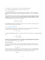
Figure 10. Spatial coherence estimates from TTMs. Vertical coherence estimates (A) are
from ADVs on TTM1 spaced 0.6m apart. Lateral coherence estimates (B) are between
neighboring TTMs spaced 50m apart. Dashed lines in both figures indicate the 95% confidence level above which the coherence estimates are statistically different from 0.
other environments (i.e. it has an exponential decay, Kilcher et al. (2014)). Unfortunately Γ∆z {u} and Γ∆z {v} are
contaminated by persistent mooring-motion contamination at 0.1Hz. The peak in coherence arises because the
measurements were made from the same TTM strongback-vane and the co-motion of that vane created a peak in the
coherence estimate at the frequency of mooring motion.
The lateral spatial-coherence estimates between ADVs on two different TTMs shows zero-spatial coherence. We
believe this to be a reliable and important result: at this site (50m water depth) and distance above the bottom (11m)
turbulence is incoherent over spatial separations of 50m. This supports the theory that the limiting scale for spatial
coherence of turbulence is controlled by the outer scale of the forcing. That is, the lateral spatial coherence is controlled by the distance from the bottom. This indicates that turbulent loading on devices in an array with hub-heights
smaller than their separation distance will be uncorrelated across the array.
5
Summary
This document outlines the methods for making turbulence measurements at HKT sites using mooring-deployed
IMU-equipped ADVs. The critical issue addressed by this approach is that ADVs–which accurately measure turbulence statistics–are deployed at heights above the sea-bed that are relevant to HKTs. Other existing approaches–most
of which deploy instrumentation on the seafloor (either ADPs, or ADVs)–do not resolve the statistics of the turbulence with sufficient accuracy (ADPs) or at the correct location (ADVs) to produce reliable device lifetime estimates.
This manual provides guidance on: 1) designing mooring hardware that can support the instrumentation, 2) planning
deployment and recovery to capture the statistics of turbulence that are important to HKTs, 3) configuring instrumentation for data collection, 4) processing data, and 5) tips for analyzing data to produce useful results. It is highly
recommended that users of this manual also download and install the DOLfYN software package, as each data processing step described herein can be performed in a few lines of code. In particular, the tedious details of accounting
for different coordinate systems have been simplified therein (appendix A).
Finally, in section 4, we demonstrate analysis methods for producing estimates of turbulent quantities that are use-
18
ful to HKT device and site developers. Most importantly, the approach outlined in this method produces reliable
estimates of the Reynold’s stresses, turbulent energy, and turbulence spectra. The w-component of vertical spatial
coherence can be estimated from a single mooring, and the research team behind this manual is developing a new,
more stable platform for measuring the u- and v-components of spatial coherence.
19
Feedback
If you have comments, questions, suggestions or corrections please contact Levi Kilcher at the National Renewable
Energy Laboratory. He will be happy to address your concerns if time and resources permit. Send comments to:
Levi Kilcher
NWTC/3811
National Renewable Energy Laboratory
1617 Cole Blvd
Golden, CO 80401-3393
United States of America
[email protected]
+1 (303) 384-7192
20
References
Commission, I.E. (2005). Wind Turbines Part 1: Design requirements.
Egeland, M.N. (2014). Spectral evaluation of motion compensated adv systems for ocean turbulence measurements.
Ph.D. Thesis, Florida Atlantic University.
Goring, D.G.; Nikora, V.I. (2002). “Despiking acoustic doppler velocimeter data.” Journal of Hydraulic Engineering
128; pp. 117–126.
Gunawan, B.; Neary, V.S.; Colby, J. (2014). “Tidal energy site resource assessment in the East River tidal strait, near
Roosevelt Island, New York, NY (USA).” Renewable Energy 71; pp. 509–517.
Jonkman, B.J. (September 2009). TurbSim user’s guide version 1.50. NREL/TP-500-46198, National Renewable
Energy Laboratory.
Kelley, N.; Hand, M.; Larwood, S.; McKenna, E. (January 2002). The NREL Large-Scale Turbine Inflow and
Response Experiment - Preliminary Results. NREL/CP-500-30917, National Renewable Energy Laboratory.
Kelley, N.D.; Jonkman, B.J.; Scott, G.N.; Bialasiewicz, J.T.; Redmond, L.S. (August 2005). The impact of coherent
turbulence on wind turbine aeroelastic response and its simulation. NREL/CP-500-38074, National Renewable
Energy Laboratory.
Kilcher, L.; Thomson, J.; Colby, J. (April 2014). “Determining the spatial coherence of turbulence at MHK sites.”
2nd Marine Energy Technology Symposium. Seattle, WA.
Kolmogorov, A.N. (1941). “Dissipation of Energy in the Locally Isotropic Turbulence.” Dokl. Akad. Nauk SSSR
32(1); pp. 16–18.
URL http://links.jstor.org/sici?sici=0962-8444%2819910708%29434%3A1890%3C15%
3ADOEITL%3E2.0.CO%3B2-C
MicroStrain, I. (). 3DM-GX3-25 Miniature Attitude Heading Reference system product datasheet. LORD Microstrain.
URL http://files.microstrain.com/3DM-GX3-25-Attitude-Heading-Reference-System-Data-Sheet.
pdf
——— (April 2012). 3DM-GX3-15,-25 MIP Data Communications Protocol. 459 Hurricane Lane, Williston, VT
05495. Www.microstrain.com/inertial/3DM-GX3-25/.
URL http://files.microstrain.com/3DM-GX3-15-25-MIP-Data-Communications-Protocol.
pdf
Nortek (August 2005). Vector Current Meter User Manual. Vangkroken 2, NO-1351 RUD, Norway, h ed.
Polagye, B.; Thomson, J. (2013). “Tidal energy resource characterization: methodology and field study in Admiralty
Inlet, Puget Sound, WA (USA).” Proceedings of the Institution of Mechanical Engineers, Part A: Journal of Power
and Energy 227(3); pp. 352–367.
Priestley, M. (1981). Spectral Analysis and time series. Academic Press.
Røstad, J. (September 2011). System Integrator Manual. Nortek AS, Vangkroken 2, NO-1351 RUD, Norway.
Stacey, M.T.; Monismith, S.G.; Burau, J.R. (1999). “Observations of Turbulence in a Partially Stratified Estuary.”
Journal of Physical Oceanography 29; pp. 1950–1970.
Thomson, J.; Kilcher, L.; Richmond, M.; Talbert, J.; deKlerk, A.; Polagye, B.; Guerra, M.; Cienfuegos, R. (2013).
“Tidal turbulence spectra from a compliant mooring.” 1st Marine Energy Technology Symposium. Washington,
DC.
21
Thomson, J.; Polagye, B.; Durgesh, V.; Richmond, M. (2012). “Measurements of turbulence at two tidal energy sites
in Puget Sound, WA.” Journal of Oceanic Engineering 37(3); pp. 363–374.
Wahl, T.L. (2003). “Discussion of "Despiking Acoustic Doppler Velocimeter Data" by Derek G. Goring and
Vladimir I. Nokora.” Journal of Hydraulic Engineering 129; pp. 484–487.
22
A
Coordinate systems
Tracking coordinate systems (‘reference frames’, or simply ‘frames’) is a critical and somewhat tedious task for
making accurate velocity measurements using moored ADVs. The coordinate systems for doing so can be broken
into two categories: 1) the ‘inertial’ or ‘stationary’ ones into which it is the goal to transform the measurements, and
2) the moving coordinate systems in which sensors make measurements. The purpose of this appendix is to clearly
document and define the relationships between all of the coordinate systems necessary for quantifying turbulence
using moored ADVs. This appendix starts with general definitions of coordinate systems and the relationships
between them (A.1), then details the stationary and measurement frames used herein (A.2 and A.3, respectively).
A.1
Defining coordinate systems
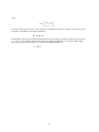
Consider two three-dimensional right-handed coordinate systems (‘a’ and ‘b’) with orthogonal basis vectors x̂a , ŷa ,
ẑa , and x̂b , ŷb , ẑb . In general, these coordinate systems are related by the equation:
~rb = Rab · (~ra − lba )
.
Here superscripts denote the coordinate system that the quantity is measured in and · indicates standard matrix
multiplication. The vectors~ra and~rb point to the same point in space, but in the two distinct coordinate systems.
In this framework the vector lba is the ‘translation vector’ that specifies the origin of coordinate system ‘b’ in the ‘a’
frame, and Rab is the ‘orientation matrix’ of ‘b’ in ‘a’. With these definitions, the following statements are true:
∙ a vector can be mapped from one coordinate system to the other by,
~ub = Rab ·~ua
.
∙ The inverse rotation is simply the transpose,
Rba = (Rab )−1 = (Rab )T
.
∙ The determinant of the rotation matrix is 1,
det(Rab ) = 1
A.2
.
Stationary frames
Throughout the main body of this document measurements are discussed in terms of two stationary coordinate
systems: a) the ‘earth frame’ is the coordinate system in which motion correction is performed15 , and b) a local
‘analysis frame’ coordinate system in which turbulence is analyzed and discussed.
A.2.1
The earth frame
The earth coordinate system is the coordinate system in-which the orientation of the ADV is measured (see A.3.2),
and is the coordinate system in-which motion correction is most easily calculated and discussed (section 3.2). This
work utilizes ‘e’ superscripts to denote an ‘ENU’ earth coordinate system with basis vectors,
x̂e : East,
ŷe : North, and
ẑe : Up.
15 No doubt the earth reference frame is not technically ‘inertial’, but for the purposes of measuring turbulence in tidal straits we consider it to
be so.
23
A.2.2
The analysis frame
The choice of ‘analysis frame’ will, in general, depend on the data available and the goals of the analysis. For quantifying inflow to HKTs it is common practice to use a coordinate system in which,
x̂: is the ‘streamwise’ or ‘flood’ direction,
ŷ: is the ‘cross-stream’ direction (defined by the right-hand rule relative to x̂ and ẑ), and
ẑ: is the ‘vertical up’ direction.
Note that throughout this work vector quantities with no superscript are in this local frame. The orientation of this
frame relative to the earth is defined as,


cos θ
sin θ 0
Se =  − sin θ cos θ 0 
.
0
0
1
Where θ is the angle from East to the ‘streamwise’ direction.
For the purpose of estimating θ it is convenient to use complex notation for the horizontal velocity,
Ũ e = ue + i ve = Ueiφ
e
.
√
Where i = −1, e ≈ 2.71828 is Euler’s number, U is the instantaneous horizontal velocity magnitude and φ e is the
angle of that velocity from east.
For measurements at locations where the flow does not change direction dramatically over the measurement period
(e.g. in rivers), the streamwise direction can be estimated simply from an average of the horizontal velocity over the
entire data record,
θriver = arg ⟨Ũ e ⟩data
.
Where ⟨⟩data denotes an average of all data, and arg returns the complex angle of its argument.
For measurements at locations where velocity changes direction over the measurement period a more sophisticated
method for determining a local coordinate system is often required. For tidal flows, for example, it is often useful to
define the ‘streamwise’ direction to be parallel with ebb and opposite flood (or vice-versa). This can be done by first
defining,
(
2φ e
for 0 < φ e < π
†
φ =
.
e
2(φ − π) for pi < φ e < 2π
That is, φ e angles in the lower-half of the unit circle are rotated to be in the opposite direction, and then all angles are
doubled so that φ † ‘fills-out’ the unit circle again. When re-combined with the velocity magnitudes, φ † , can be used
to estimate the ebb-flood direction as,
†
θtide = arg ⟨Ueiφ ⟩data /2
.
The ambiguity over whether θtide points in the direction of ebb or flood can easily be resolved by knowledge of the
tidal-geographic context of the measurements.
A.3
Measurement frames
To combine signals from an IMU with those of an ADV to perform motion correction the coordinate systems in
which each of the measurements are made must be carefully accounted for.
24
Notch in end-cap
Figure 11. The circuit-board and pressure-case end-cap of a Nortek Vector equipped with a Microstrain
IMU. The ADV-body coordinate system (yellow) is depicted on the right. The notch in the end-cap defines the x̂* direction (out of the page), and the ẑ* direction points back along the pressure case axis.
A zoom-in on the Microstrain chip highlights its coordinate system (magenta) relative to the body.
For the Nortek Vector instruments that were used for this work the ‘ADV-body’ coordinate system is defined as being
centered on the cylinder-body axis at the point where the head-cable meets its end-cap. The basis vectors of this
coordinate system are defined as (Figures 11 and 12B):
x̂* : points from the center of the ‘head’ end-cap toward the notch in that end-cap,
ŷ* : is defined by the right-hand-rule based on the other two basis vectors, and
ẑ* : points from the ‘head’ end-cap toward the ‘battery’ end-cap along the body-cylinder (pressure case) axis.
A.3.1
The ADV head
In order to transform measured velocities into a meaningful reference frame (and to perform motion correction) the
orientation (and position) of the ADV head in terms of the body coordinate system must be known. To facilitate this
* , are defined according to,
the orientation matrix of the ADV head, H, and translation vector16 , ~lhead
*
~xhead = H · (~x* −~lhead
)
,
(5)
where ~xhead and ~x* are the same point in the head and body coordinate systems, respectively. Combined with the
math notes in the previous section, the velocity vectors in the head frame can be transformed into the body frame by,
~u* = HT ·~uhead
.
For Nortek Vectors, the coordinate system of the ADV head is centered on the transmit transducer face, and the
coordinate-directions are defined by (Figure 12B, Nortek (2005)):
16 The
position of the ADV-head origin (transmit transducer) in the body coordinate system.
25
(6)
x̂head : the direction of one of the transducer ‘receive’ arms (marked with tape or paint)
ŷhead : is defined by the right-hand-rule based on the other two basis vectors, and
ẑhead : is into the transducer face.
For fixed-head Nortek Vector ADVs, the body-frame and head-frame have parallel coordinate systems (H is the
*
identity matrix), and the ‘head-frame’ is translated 21cm along the z-axis. That is, ~lhead
= (0, 0, −0.21)m (Nortek,
2005).
For cable-head ADVs, the position and orientation of the ADV head is arbitrary. This means that when preparing to
make measurements using cable-head ADVs, the orientation and position of the ADV head must be accurately
recorded in order to allow the ADV measurements to be transformed into the body frame during post-processing.
*
For the example in Figure 12A, ~lhead
= (254, 64, −165) mm, and


0
0 −1
.
H =  0 −1 0 
−1 0
0
In general H will not necessarily be symmetric nor will it have so many zero-elements (i.e. these characteristics are
specific to the head-body alignment of the example).
A.3.2
The IMU coordinate system
Like the ADV head, the coordinate system in which the IMU measurements are made must be clearly defined and
documented. In general, the IMU frame is related to the body coordinate system by,
*
~ximu = A · (~x* −~limu
)
.
* = (0.006, 0.006, 0.150)m
For the Microstrain 3DM-GX3-25 (IMU) as it is integrated into the Nortek Vector (Figure 11), ~limu
and,


0 0 1
A= 0 1 0 
.
−1 0 0
The DOLfYN software package automatically rotates all IMU vectors so that orientation and motion data returned
by dolfyn.io.read_nortek is in the ADV body frame (see the dolfyn.io.nortek.NortekReader.sci_microstrain source
* to ~l *
~*
code for details). DOLfYN also adds ~limu
head to estimate ` .
The orientation matrix
In order to use the orientation matrix to rotate velocity measurements into an earth-fixed coordinate system it is
important to understand how the orientation matrix is defined. The Microstrain IMU outputs an orientation matrix,
Rimu , such that:
~uimu = Rimu ·~uNED
.
Where ~uimu and ~uNED are vectors in the IMU’s local coordinate system and a ‘north-east-down’ (NED) earth-fixed
coordinate system, respectively (MicroStrain, 2012). However, this NED earth coordinate system is different from
the ENU earth coordinate system used here (and typically used by Nortek (Røstad, 2011)). That is,
~u = B ·~uNED
,
26
Marked Arm
A
B
Figure 12. Coordinate systems of the ADV body and head. A) A strongback with an ADV rests on a
block of wood. Coordinate systems of the ADV head (magenta) and body (yellow) are shown. The
x̂head -direction is known by the black-band around the transducer arm, and the x̂* direction is marked
by a notch on the end-cap (indiscernible in the image). The cyan arrow indicates the body-to-head
* . The perspective slightly distorts the fact that x̂head ‖ −ẑ* , ŷhead ‖ −ŷ* , and ẑhead ‖ −x̂* .
vector, ~lhead
B) Coordinate system of the ADV head as defined in the Nortek Vector manual (Nortek, 2005).
27
where,

0
B= 1
0
1
0
0

0
0 
−1
.
From this, and the above discussion of the orientation of the IMU in the ADV, it is simple to show that the orientation matrix of the ADV body in a ENU earth frame is,
R = A · Rimu · B
,
The DOLfYN software package makes this transformation when reading the orientation matrix from Nortek Vector
‘.vec’ files (i.e. the ‘orientmat’ attribute in the data object returned by DOLfYN’s io.read_nortek is R, not Rimu ).
This way vectors in the body frame can be rotated into the ENU earth frame by,
~u = RT ·~u*
.
28
B
Filtering Acceleration
Bench-tests of the Microstrain IMU indicate that its accelerometers drift for frequencies < 10−2 Hz (a minute or
more, Egeland (2014)). Therefore, in order to remove bias-drifts in ~a that–when integrated according to (2)–lead to
large errors in ~uea this document recommends using fa = 0.033Hz (30seconds). On the other hand, real motions at
and below fa will not be accurately accounted for in ~uea , and will therefore persist as low-frequency motion contamination not corrected-for in the estimate of ~u.
For moorings whose low-frequency motion is limited by the mooring line itself this is a reasonable approach. Assuming that the displacement of the ADV head (from the mooring’s neutral position) is likely to be < 20% of its
distance from the bottom, then for ADVs deployed at 10m depth the speed of their low-frequency motion (i.e. below fa = 0.03 Hz) will be < 0.07m/s. In other words, for a 10m mooring the choice of fa = 0.03Hz allows for
low-frequency motion contamination on the order of 7cm/s to persist. This is a notable but relatively minor level of
uncertainty in the context of the highly energetic flows that exist at tidal energy sites.
29
C
DOLfYN data processing scripts
The following script details data processing steps.
adv_example01.py
1
2
3
# To get started first import the DOLfYN ’adv’ advanced programming
# interface (API):
from dolfyn.adv import api as adv
4
5
6
7
8
# Import matplotlib tools for plotting the data:
from matplotlib import pyplot as plt
from matplotlib import dates as dt
import numpy as np
9
10
11
##############################
# User input and customization
12
13
14
# The file to load:
fname = ’./data/vector_data_imu01.vec’
15
16
17
18
# This is the vector from the ADV head to the body-frame, in meters,
# in the ADV coordinate system.
body2head_vec = np.array([0.48, -0.07, -0.27])
19
20
21
22
23
# This is the orientation matrix of the ADV head relative to the body.
# In this case the head was aligned with the body, so it is the
# identity matrix:
body2head_rotmat = np.eye(3)
24
25
26
27
28
29
30
31
# The time range of interest.
t_range = [
# The instrument was in place starting at 12:08:30 on June 12,
# 2012.
dt.date2num(dt.datetime.datetime(2012, 6, 12, 12, 8, 30)),
# The data is good to the end of the file.
np.inf]
32
33
34
# This is the filter to use for motion correction:
accel_filter = 0.1
35
36
37
# End user input section.
###############################
38
39
40
# Read a file containing adv data:
dat_raw = adv.read_nortek(fname)
41
42
43
44
45
# Crop the data for t_range using DOLfYN’s ’subset’ method (creates a
# copy):
t_range_inds = (t_range[0] < dat_raw.mpltime) & (dat_raw.mpltime < t_range[1])
dat = dat_raw.subset(t_range_inds)
46
47
# Then clean the file using the Goring+Nikora method:
30
48
49
adv.clean.GN2002(dat)
dat_cln = dat.copy()
50
51
52
53
54
55
####
# Create a figure for comparing screened data to the original.
fig = plt.figure(1, figsize=[8, 4])
fig.clf()
ax = fig.add_axes([.14, .14, .8, .74])
56
57
58
# Plot the raw (unscreened) data:
ax.plot(dat_raw.mpltime, dat_raw.u, ’r-’)
59
60
61
62
63
64
65
66
67
68
69
# Plot the screened data:
ax.plot(dat.mpltime, dat.u, ’g-’)
bads = np.abs(dat.u - dat_raw.u[t_range_inds])
ax.text(0.55, 0.95,
"%0.2f%% of the data were ’cleaned’\nby the Goring+Nikora method." %
(np.float(sum(bads > 0)) / len(bads) * 100),
transform=ax.transAxes,
va=’top’,
ha=’left’,
)
70
71
72
73
74
75
76
77
78
79
80
81
82
83
84
# Add some annotations:
ax.axvspan(dt.date2num(dt.datetime.datetime(2012, 6, 12, 12)),
t_range[0], zorder=-10, facecolor=’0.9’,
edgecolor=’none’)
ax.text(0.13, 0.9, ’Mooring falling\ntoward seafloor’,
ha=’center’, va=’top’, transform=ax.transAxes,
size=’small’)
ax.text(t_range[0] + 0.0001, 0.6, ’Mooring on seafloor’,
size=’small’,
ha=’left’)
ax.annotate(’’, (t_range[0] + 0.006, 0.3),
(t_range[0], 0.3),
arrowprops=dict(facecolor=’black’, shrink=0.0),
ha=’right’)
85
86
87
88
89
90
91
92
93
# Finalize the figure
# Format the time axis:
tkr = dt.MinuteLocator(interval=5)
frmt = dt.DateFormatter(’%H:%M’)
ax.xaxis.set_major_locator(tkr)
ax.xaxis.set_minor_locator(dt.MinuteLocator(interval=1))
ax.xaxis.set_major_formatter(frmt)
ax.set_ylim([-3, 3])
94
95
96
97
98
# Label the axes:
ax.set_ylabel(’$u\,\mathrm{[m/s]}$’, size=’large’)
ax.set_xlabel(’Time [June 12, 2012]’)
ax.set_title(’Data cropping and cleaning’)
31
99
100
ax.set_xlim([dt.date2num(dt.datetime.datetime(2012, 6, 12, 12)),
dt.date2num(dt.datetime.datetime(2012, 6, 12, 12, 30))])
101
102
103
104
105
# Save the figure:
fig.savefig(’./fig/crop_data.pdf’)
# end cropping figure
####
106
107
108
109
110
111
# Perform motion correction (including rotation into earth frame):
dat.props[’body2head_vec’] = body2head_vec
dat.props[’body2head_rotmat’] = body2head_rotmat
mc = adv.motion.CorrectMotion(accel_filter)
mc(dat)
112
113
ax.plot(dat.mpltime, dat.u, ’b-’)
114
115
116
117
# Then rotate it into a ’principal axes frame’:
adv.rotate.earth2principal(dat)
adv.rotate.earth2principal(dat_cln)
118
119
120
121
122
# Define an averaging object, and create an ’averaged’ data set:
binner = adv.TurbBinner(n_bin=19200, fs=dat.fs, n_fft=4096)
dat_bin = binner(dat)
dat_cln_bin = binner(dat_cln)
123
124
125
# At any point you can save the data:
dat_bin.save(’adv_data_rotated2principal.h5’)
126
127
128
# And reload the data:
dat_bin_copy = adv.load(’adv_data_rotated2principal.h5’)
129
130
131
132
133
134
####
# Figure to look at spectra
fig2 = plt.figure(2, figsize=[6, 6])
fig2.clf()
ax = fig2.add_axes([.14, .14, .8, .74])
135
136
137
138
139
ax.loglog(dat_bin.freq, dat_bin.Suu_hz.mean(0),
’b-’, label=’motion corrected’)
ax.loglog(dat_cln_bin.freq, dat_cln_bin.Suu_hz.mean(0),
’r-’, label=’no motion correction’)
140
141
142
143
# Add some annotations
ax.axhline(1.7e-4, color=’k’, zorder=21)
ax.text(2e-3, 1.7e-4, ’Doppler noise level’, va=’bottom’, ha=’left’,)
144
145
146
147
148
149
ax.text(1, 2e-2, ’Motion\nCorrection’)
ax.annotate(’’, (3.6e-1, 3e-3), (1, 2e-2),
arrowprops={’arrowstyle’: ’fancy’,
’connectionstyle’: ’arc3,rad=0.2’,
’facecolor’: ’0.8’,
32
’edgecolor’: ’0.6’,
},
150
151
152
153
ha=’center’,
)
154
155
156
157
158
159
160
161
162
ax.annotate(’’, (1.6e-1, 7e-3), (1, 2e-2),
arrowprops={’arrowstyle’: ’fancy’,
’connectionstyle’: ’arc3,rad=0.2’,
’facecolor’: ’0.8’,
’edgecolor’: ’0.6’,
},
ha=’center’,
)
163
164
165
166
167
168
# Finalize the figure
ax.set_xlim([1e-3, 20])
ax.set_ylim([1e-4, 1])
ax.set_xlabel(’frequency [hz]’)
ax.set_ylabel(’$\mathrm{[m^2s^{-2}/hz]}$’, size=’large’)
169
170
171
f_tmp = np.logspace(-3, 1)
ax.plot(f_tmp, 4e-5 * f_tmp ** (-5. / 3), ’k--’)
172
173
174
175
176
177
178
179
ax.set_title(’Velocity Spectra’)
ax.legend()
#ax.axhspan(1e-4, 3e-4, facecolor=’w’, alpha=0.8, zorder=10, edgecolor=’none’)
ax.axvspan(1, 16, 0, .2, facecolor=’0.8’, zorder=-10, edgecolor=’none’)
ax.text(4, 4e-4, ’Doppler noise’, va=’bottom’, ha=’center’,
#bbox=dict(facecolor=’w’, alpha=0.9, edgecolor=’none’),
zorder=20)
180
181
fig2.savefig(’./fig/motion_vel_spec.pdf’)
33
Data cropping and cleaning
3
2
1
u [m/s]
0.41% of the data were 'cleaned'
by the Goring+Nikora method.
Mooring falling
toward seafloor
Mooring on seafloor
0
1
2
3
12:00
12:05
12:10
12:15
12:20
Time [June 12, 2012]
12:25
12:30
Figure 13. The ‘crop_data.pdf’ figure generated by the adv_example01.py script. The
uncropped, uncleaned data is in red, and the cropped and cleaned data is in blue.
34
Velocity Spectra
motion corrected
no motion correction
100
[m2 s−2 /hz]
10-1
Motion
Correction
10-2
10-3
Doppler noise
Doppler noise level
10-4 -3
10
10-2
10-1
100
frequency [hz]
101
Figure 14. The ‘motion_vel_spec.pdf’ figure generated by the adv_example01.py script. Spikes
in the spectra due to motion contamination (red) are removed by motion correction (blue).
35