Download Clarifications and Additional Instructions For Text Problem 1

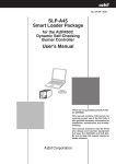
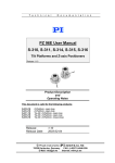
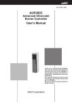
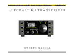
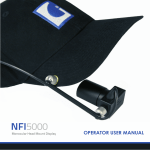
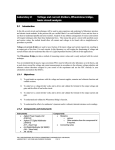
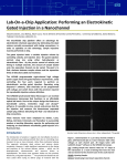
Whites
EE 322 Electronics II – Wireless Communication Electronics
Page 1 of 37
Clarifications and Additional Instructions
For Text Problem 1
Problem 1 – RESISTORS
Remember to work out all text problems in your laboratory notebook, whether or not they
require actual laboratory work. You’ll make copies of all the pages for each of your
problems, and turn these in on the due date.
Also remember to number the front of all pages in the upper right-hand corner before using
your notebook.
South Dakota School of Mines and Technology
rev. 1/17/06
Whites
EE 322 Electronics II – Wireless Communication Electronics
Page 2 of 37
Clarifications and Additional Instructions
For Text Problems 2, 3, and 4
Problem 2 – SOURCES
The 12-V, 0.8-A-hr battery and corresponding connectors can be found on the shelves in
room EP 126, which is one of the side rooms accessible from EP 127. Other specialized
equipment and parts for this course will also be located on those shelves.
2.A It is not necessary to use the top and bottom rows of holes if that confuses you.
2.B Develop the equivalent circuit for the battery based on your plot from part 2.A.
2.C Assume that your (real) battery is connected to the NorCal 40A.
Problem 3 – CAPACITORS
3.A Use a long BNC-to-microclip cable from the output of the oscilloscope. Do not use
the short “break out” cable as shown in Fig. 2.25 of the text. Also, do not use an
oscilloscope probe yet. That will happen later in part 3.G.
When the text says to set the source to 1 Vpp that means the displayed voltage on the
Agilent 33120A Arbitrary Waveform Generator (AWG) should read 1 Vpp. As stated
in the text and discussed in class, the voltage shown on the display of the AWG
equals the output voltage only if the load is 50 Ω.
Sketch the circuit in you lab book which corresponds to what is drawn in Fig. 2.25.
3.F The equivalent input circuit for the Tektronix TDS 2012 oscilloscope is 1 MΩ ±2%
in parallel with 20 pF ±3 pF. See the User Manual for this and other information on
the scope. (This manual, and manuals for other equipment, can be found on the EE
322 web page.)
Compute the cable capacitance in pF/ft.
3.G Now use the Tektronix P2220 Voltage Probe. Make certain that the Attenuation
Switch on the probe handle has been set to the 10X position, and that on the
oscilloscope the Probe option has been set to 10X as well. From the Tektronix TDS
2012 and P2220 User Manuals, the probe equivalent circuit is 10 MΩ in parallel with
16 pF. These values are also listed on the probe assembly.
Use a TENMA 72-410A (or equivalent) multimeter to measure the resistance of the
cable. This resistance is too large to be accurately measured with a less-capable
DMM.
3.H As stated above, the total capacitance “marked on the probe” is 16 pF. Make sure to
show all of your work.
3.I Make these measurements from the circuit in part 3.E. (Note that unless otherwise
stated, the text questions assume your circuit is unchanged from the previous part.)
3.J Draw the circuit including the probe. For the time constant, determine the Thévenin
South Dakota School of Mines and Technology
rev. 1/17/06
Whites
EE 322 Electronics II – Wireless Communication Electronics
Page 3 of 37
resistance seen by the total capacitance of the probe (16 pF). (The predicted value
may vary by 10% from the measured value.)
Problem 4 – DIODE DETECTORS
Connect the “sync” output from the Agilent 33120A to “EXT TRIG” on the scope. Set the
Agilent 33120A to a frequency of 1 MHz. For AM, press Shift/AM on the 33120A. Set the
modulating frequency to 1 kHz by pressing Shift/Freq. Set the modulation depth of 70% by
pressing Shift/Level and entering 70.
Next, adjust the scope for two-channel input. Set the time scale so that the output (ch. 2)
shows approximately two periods of the modulated signal. Press TRIG MENU and select Ext
Triggering.
Finally, adjust the amplitude of the input signal to 5 Vpp.
4.A The unlabelled electrical parts in Fig. 2.29 are described in Appendix A of the text.
This appendix is a very good reference for this, and other, text problems.
South Dakota School of Mines and Technology
rev. 1/17/06
Whites
EE 322 Electronics II – Wireless Communication Electronics
Page 4 of 37
Clarifications and Additional Instructions
For Text Problems 5-7
Problem 5 – INDUCTORS
A BNC cable should connect the output of the arbitrary waveform generator to a BNC tee
connected to ch. 1 of the scope. A BNC-to-alligator-clip cable is connected from the tee to
the circuit. A second tee should be connected to ch. 2 of the scope. A 50-Ω BNC load
(sometimes called a “termination”) should be connected to one output of this ch. 2 tee and
the other connected to the output of the circuit through a second BNC-to-alligator-clip cable.
Make certain your oscilloscope has properly detected the attenuation switch setting on the
probe (1x or 10x) before making measurements. If it hasn’t, you can manually select the
proper setting after pushing the CH 1 MENU or CH 2 MENU button depending on which
channel the probe is attached. (The Probe Check Wizard can also be used by pushing the
PROBE CHECK button.)
5.B Remember that the Agilent 33120A has an internal source resistance of 50 Ω.
The pinout of the 2N2222A is shown in its data sheet located in Appendix D of the text. Note
that there is an error in this data sheet and the E and C terminals are reversed from what is
shown.
The power supply in Fig. 2.31 is the CSi/SPECO 13.8 Vdc unit located in EP 126. These
supplies were originally unregulated, but have been modified to provide a regulated output
voltage. Because of this, make sure you measure the supply voltage. Please report any
excessive voltages to the TAs or Mr. Dennis Rush, the ECE department technician. (Later,
when you connect this supply to your NorCal 40A, an excessive voltage could cause damage
to the radio.)
Connect a BNC cable from the 33120A to a tee on ch. 1 of the scope. A BNC-to-alligatorclip cable should run from the tee to the 2-kΩ resistor connected to the base of the transistor.
After constructing the circuit shown in Fig. 2.31, download (or sketch) the input (ch. 1) and
output (ch. 2) voltages.
5.C The “circuit capacitance” mentioned at the end of this problem is discussed later in
Prob. 6.
Problem 6 – DIODE SNUBBERS
6.B Remember that the oscilloscope input is single ended. This means that the alligator
clip hanging off the probe is earth ground. Consequently, we can’t make an inductor
voltage measurement using a single channel of the scope. We need to use both
South Dakota School of Mines and Technology
rev. 1/17/06
Whites
EE 322 Electronics II – Wireless Communication Electronics
Page 5 of 37
channels and use subtraction in, for example, a ch. 1 minus ch. 2 measurement.
Unfortunately, ch. 1 of the scope is not available.
6.C Use VL=LdI/dt and the text discussion to compute the diode “on-time.”
6.D This measured “on-time” of the diode should be quite close to your prediction in 6.C
(within approximately 10%).
Problem 7 – PARALLEL-TO-SERIES CONVERSION
7.A There is more than one way to do this problem. I did it another way than mentioned
in the text. At the end of your analysis, however, you should verify that your
expressions satisfy Qs = Qp.
South Dakota School of Mines and Technology
rev. 1/17/06
Whites
EE 322 Electronics II – Wireless Communication Electronics
Page 6 of 37
Clarifications and Additional Instructions
For Text Problems 8 and 9
Problem 8 – SERIES RESONANCE
The brown band on the inductor may have a red tinge.
You may wish to leave a few millimeters of component lead wire remaining on the front or
back of the PCB before you solder and trim. This allows you room to easily clip test leads to
the component. Once you are finished measuring, trim the leads flush to the solder bead
using side cutters. Use safety glasses or other safe methods of shielding your eyes when
trimming!
Refer to Appendix A in the NorCal40A Assembly Manual for parts descriptions and sketches.
8.A Note that L1 and C1 are connected together by a trace on the PCB. Not all traces are
located on the bottom of the PCB. A few are located on the top. This will be
important later in the course.
8.E Determine the measured Q of this circuit once you have constructed the plot.
Note that rejection factors are usually defined as ratios of powers, as in Ch. 1. Of course, use
(3.125) for your calculations here.
8.F
Contrary to what’s mentioned in the text, I had no trouble measuring Vam at 1 MHz
using Vin = 1 Vpp.
Problem 9 – PARALLEL RESONANCE
Note that the manufacturer may have replaced all 5-pF ceramic capacitors in the NorCal 40A
kit with 4.7-pF ones.
Remember to leave a few mm of component leads before soldering and trimming. You may
need these to easily connect probes.
See p. 10 in the NorCal40A Assembly Manual for a toroid-winding tutorial. It is important
that you develop the habit of winding the toroids as illustrated in the tutorial and in the text.
This will be even more important later when you wind your own RF transformers.
You need a small piece of fine sandpaper (600 or so grit wet/dry) to clean the varnish off the
ends of the magnet wire before soldering. Tin the ends of the wire before soldering the
component to the board. That way you’ll be able to see if you’ve completely removed the
South Dakota School of Mines and Technology
rev. 1/17/06
Whites
EE 322 Electronics II – Wireless Communication Electronics
Page 7 of 37
varnish. Not removing ALL of the varnish will likely cause big problems (e.g. through poor
ohmic contact), which may even be an intermittent problem.
9.C The output voltage will be larger than the input voltage. This is acceptable here since
the output is the voltage across reactive circuit elements. (This would NOT be
acceptable if the output voltage were measured across a resistor!) Large voltages
across reactive elements are a common characteristic of resonant circuits when the
frequency of operation is near resonance, as we saw in the Lecture 5 notes.
9.E I used simple voltage division to calculate the output voltage. Of course, the Norton
equivalent mentioned in the text can be helpful to analyze this circuit, as we saw in
lecture.
9.H Impedance of capacitors and inductors, of course, varies with frequency. This is what
the text is referring to when it says “…the circuit quantities vary with frequency.”
9.I Remember that with this configuration, there would no longer be an effective parallel
resistance, since with C37 removed the “topology” of the resonant circuit has
changed. It is amazing how much the Q is affected.
Make measurements of this second case by connecting the function generator to C38
and bypass C37. The fl measurement and your prediction with C37 removed should
be very close.
South Dakota School of Mines and Technology
rev. 1/17/06
Whites
EE 322 Electronics II – Wireless Communication Electronics
Page 8 of 37
PROBLEM 13 – HARMONIC FILTER*
Revised for EE 322
The Power Amplifier in the NorCal40A produces a 7-MHz carrier with 2 W of power. In
addition, the amplifier produces a small amount of power at the harmonic frequencies 14, 21 and
28 MHz. Signals at the wrong frequencies are called spurious emissions, or spurs for short. Spurs
are bad, because they interfere with other radio services. The Federal Communications
Commission (FCC) sets limits on spurs. For HF transmitters with an output of less than 5 W,
each spur must be at least 30 dB below the carrier.
The NorCal 40A has a low-pass ladder filter to reduce the harmonics, consisting of the
toroidal inductors L7 and L8 and the disk capacitors C45, C46, and C47 (Figure 5.17). The
inductors use the same T37-2 cores as the Transmit Filter. These are the cores with red paint.
However, they have only 18 turns, and this lets us use thicker wire (#26 instead of #28 magnet
wire) to accommodate the large transmitter currents. Start with a 30-cm piece of wire for each
core. Solder in the filter components, leaving the C45 leads partly exposed so that you can attach
test hooks. Also, solder on the BNC Antenna Jack J1. The two small pins are the electrical
connections, and the two large pins are the mechanical connections. Solder all four pins to the
board.
L7
Input
from
Power
Amplifier
C45
330pF
L8
C46
820pF
C47
330pF
Output to
Antenna
Jack J1
Figure 5.17. NorCal 40A Harmonic Filter.
Attach the function generator across C45 with test hooks, making sure the ground clip is
connected to the ground lead of the capacitor. Connect the oscilloscope coaxial cable to the
Antenna Jack J1. You should use a parallel 50-Ω termination on the scope.
We wish to measure the loss L of this filter, but as defined in (5.1) this involves the
measurement of time average power. This is a complicated measurement often involving
specialized instruments. There is an easier way, however, which uses only basic lab instruments.
From the Lecture 2 class notes, the open circuit output voltage from the AWG is 2Vd, where Vd is
the displayed voltage. The maximum available power from the AWG is then
( 2Vd )
=P=
2
Vd2
Pav
=
(1)
i
8Rs
2 Rs
assuming sinusoidal voltages. For a doubly terminated filter, the time-average power delivered to
the “load” (or the circuitry connected to the output of the filter) will then be
V2
P=
(2)
2 Rs
where V is the peak-to-peak, sinusoidal output voltage. From (5.1), then
South Dakota School of Mines and Technology
rev. 1/17/06
Whites
EE 322 Electronics II – Wireless Communication Electronics
L=
Page 9 of 37
2
Pi Vd ( 2 Rs )
= 2
P V ( 2 Rs )
⎛V ⎞
(3)
L = 20 log10 ⎜ d ⎟ [dB]
⎝V ⎠
Because the internal source impedance and the terminating impedance are equal and purely
resistive, we can use (3) to easily compute the filter loss factor L at some frequency from the
displayed voltage on the AWG and the amplitude of the measured output voltage.
or
A. Set the function generator amplitude to 10 Vpp. Measure the output voltage at 7 MHz and 14
MHz and use (3) to compute L in dB at these frequencies. Assuming this is a Butterworth
low-pass filter, compute the 3-dB cutoff frequency.
B. From the manufacturer’s inductance constant, Al = 4.0 nH/turn2, calculate the inductance of
L7 and L8.
C. Now use Advanced Design System (ADS) to simulate the filter response from 0 to 28 MHz
(the fourth harmonic). Instructions for running ADS can be found in the document “Getting
Started With ADS.” Apply a matched voltage source to this filter when terminated in 50 Ω.
Plot the loss factor in dB over the specified frequency range. Find the loss in dB at 7 MHz
and at 14 MHz. Print a hardcopy of this plot.
In addition to reducing the harmonics, the filter sets the load impedance for the Power
Amplifier. The output power of amplifiers often varies inversely with the impedance, so that
halving the impedance will double the output power. In addition, having a small inductive
component often improves the efficiency, by helping the amplifier approach a Class-E operating
condition, where little power is lost in switching the transistor on and off.
D. You can use ADS to easily compute the input impedance to the filter. See the document
“Getting Started With ADS” for information on how to make this calculation. Find the input
impedance of the filter at 7 MHz.
E. Assume that we would like to double the output power. You should adjust the components
in the filter so that the impedance is cut in half. There are many components that you could
change, but to make this problem specific, try varying only L7 and C46. For the capacitor,
you should stick to values in the standard 5% series, where the first two digits of the
capacitance come from this list: 10, 11, 12, 13, 15, 16, 18, 20, 22, 24, 27, 30, 33, 36, 39, 43,
47, 51, 56, 62, 68, 75, 82, and 91. Otherwise, you would not be able to buy the capacitors.
For the inductor, use only values that you can achieve by adding or subtracting turns from
your cores. What values of L7 and C46 give an impedance closest to half the original
impedance?
F. We can improve the harmonic rejection by allowing more ripple. Using the filter table,
design a 5th-order, 0.2-dB ripple Chebyshev low pass filter with fc = 8 MHz. Specify the
South Dakota School of Mines and Technology
rev. 1/17/06
Whites
EE 322 Electronics II – Wireless Communication Electronics
Page 10 of 37
closest 5% capacitor values and the closest number of turns that you can get with T37-2
cores. Simulate your design with ADS and make a plot of the filter loss. (“Your design”
means this fifth-order Chebyshev filter constructed using standard 5% capacitor values and
wound inductors with integer numbers of turns.) What is the loss in dB at 7 MHz and 13
MHz?
* From D. B. Rutledge, The Electronics of Radio. Cambridge, UK: Cambridge University
Press, 1999.
South Dakota School of Mines and Technology
rev. 1/17/06
Whites
EE 322 Electronics II – Wireless Communication Electronics
Page 11 of 37
PROBLEM 14 – IF FILTER*
Revised for EE 322
The IF Filter in the NorCal 40A is a 4-element Cohn filter (Figure 5.18). Study the endpaper
to see how this filter is connected in the receiver. The filter uses quartz crystals for
microprocessor clocks. They are quite inexpensive, costing only about a dollar, but
unfortunately, as they come from the dealer, the resonant frequencies are not nearly close enough
together to make a good filter. Wilderness Radio sorts crystals for the NorCal 40A so that they
match within 20 Hz. You need six matched crystals in all, four for the IF Filter now, and two for
mixer oscillators later.
X1
All
capacitors
270 pF
C9
X2
X3
X4
C10
C11
C12
C13
Figure 5.18. The IF Filter in the NorCal 40A.
A. First we measure the resonant frequency of the crystals with the setup shown in Figure 5.19.
Number each of your crystals from 1 to 6 using an indelible marker. The function generator
should be set to a 4,913,500-Hz sine wave (or perhaps near the frequency stamped on your
crystal, if there is one) with an amplitude setting of 0.5 Vpp. You should set up the function
generator so you can change the frequency in intervals of 1 Hz.
Because the crystals have a series resonance, we can recognize the resonant frequency by a
dip in the oscilloscope voltage as we vary the frequency. Find the frequency to the nearest
hertz that gives the minimum voltage on the scope. Measure and record the resonant
frequency of all six crystals. Use the four with the closest resonant frequencies for your IF
Filter. Is the variation of your resonant frequencies within Wilderness Radio’s specification
of ±20 Hz?
South Dakota School of Mines and Technology
rev. 1/17/06
Whites
EE 322 Electronics II – Wireless Communication Electronics
Page 12 of 37
Figure 5.19. Setup for testing crystals.
B. Next we will find the components of an equivalent electrical circuit for a crystal, starting
with the resistance. (Perform these and future crystal measurements in this problem for just
one of the four quartz crystals from 14.A.) Use the equivalent circuit shown in Figure 5.20.
Record the output voltage V at resonance and use it to calculate the crystal resistances R. Pay
close attention to the difference between a loaded Q and an unloaded Q.
+
50 Ω
1 Vpp
L
C
V
Scope
R
-
Figure 5.20. Equivalent circuit for the crystal and generator.
C. When we shift the frequency off resonance, the scope voltage will increase. Calculate the
scope voltage Vx that we would expect when the crystal reactance is equal to R. Notice that
this is not simply 2 times the minimum voltage, because the crystal resistance is
comparable to the resistance of the function generator. Now measure the upper and lower
frequencies fu and fl that give a scope voltage equal to Vx. Calculate the Q of the crystal from
the bandwidth ∆f = fu − f l and the resonant frequency f0. You need to be careful about the
Q here. The crystal Q only includes the resistance of the crystal. It is different from the
circuit Q, which also includes the resistance of the generator and is lower because of it.
Often people call the crystal Q the unloaded Q, and the circuit Q the loaded Q.
D. Now calculate the equivalent inductance and capacitance of the crystal. One thing that you
need to be careful about here is that we do not have a precise measurement of either L or C
individually, but we know their product extremely precisely through the resonant frequency.
For one of the components you should use only the number of significant digits that makes
sense from your scope measurement, but for the other you will need to use seven significant
digits, so that the product will give the correct resonant frequency. Check with a calculator
that the product of your L and C values gives the resonant frequency correctly to seven
digits. Otherwise, the filter pass band will shift clear off the screen in the ADS simulation.
E. Make a model of the Cohn filter with ADS, using the equivalent circuit model for the crystal
that you have developed and 270-pF capacitors. You should use a range of 2.5 kHz for
frequency and 0 to 60 dB for the loss factor. Assume that the filter sees an impedance of 200
Ω. Make a plot of the loss factor.
South Dakota School of Mines and Technology
rev. 1/17/06
Whites
EE 322 Electronics II – Wireless Communication Electronics
Page 13 of 37
F. Investigate the effect of changing the impedance the filter sees to 50 Ω. Make a plot of the
loss factor and describe the behavior qualitatively.
G. Return the impedance level to 200 Ω and investigate the effect of changing the capacitors to
200 pF. Make a plot and describe the behavior qualitatively.
H. In your simulation, return the capacitance to 270 pF. What is the minimum loss in dB in the
pass band?
I.
One important job of the IF Filter is to reject interference at the upper-sideband frequency,
1,240 Hz above the signal frequency. We hear the upper-sideband frequency as a tone of the
same pitch as the signal, and so our ears cannot distinguish the interference from the signal.
This is called a spurious response, or spur for short. The upper-sideband frequency is a
difficult spur to reject because it is so close to the signal. In the ADS simulation, what is the
upper-sideband rejection? What do we normally call the signal that exists 1,240 Hz above
the signal frequency coming out of the RF Mixer?
Now build the filter. Solder in the 270-pF disk capacitors (C9 through C13). If your kit came
with them, slide a plastic spacer onto the leads of each of the four crystals, all the way up against
the metal case. Now install the filter crystals (X1 through X4) close to the board. The metal cases
of the crystals are not connected to the leads or to any other part of the circuit yet. We say that
the cases are floating. It is a bad idea to leave large pieces of metal in a circuit floating, because
signals can couple capacitively through the metal pieces between different parts of the circuit and
end up where you do not want them. To avoid this coupling, we connect each can to ground.
There is a small ground hole in the board between the crystals to make this easy. Use bare #22
wire to connect the crystal cans. Figure 5.21 shows how you can do this. Connect the cans with a
wire running along the top. It may help to gently bend the cans toward each other until the space
between them is small. You should use large solder beads, and make sure that the top of the cans
gets quite hot so that the solder beads stick well to the cans. If the cases are not hot enough, the
wire and solder will pop off the cans. Then solder a wire to the ground hole, hook the other end
to the top wire, and solder them together.
Figure 5.21. Crystal metal cases and the ground connections.
The filter is designed for a 200-Ω generator and load. We will add resistors to give the
function generator and scope this resistance (Figure 5.22). For the load, solder a 200-Ω resistor
South Dakota School of Mines and Technology
rev. 1/17/06
Whites
EE 322 Electronics II – Wireless Communication Electronics
Page 14 of 37
from the left L4 hole (connecting to C13 at the filter output) to the left C14 hole, which is a
ground connection. Connect the scope across the 200-Ω resistor. The scope connection should be
as short as possible, or else the capacitance of the cable will affect the shape of the filter
response. The best thing to do is to use a “breakout” for the connections to channel 1 of the
scope. The breakout is a BNC-to-microclip connection with no cable. For the function-generator
connection, solder one end of a 150-Ω resistor to the number-3 hole of T3. Attach the functiongenerator red lead to the other end of the 150-Ω resistor (Figure 5.22). The ground lead can be
attached to C10 on the ground side.
Figure 5.22. Resistor connections to the crystal filter.
J.
With an amplitude setting of 0.5 Vpp, measure the minimum loss in dB of the filter to
compare with the ADS simulation.
K. Next we make a plot of the loss in dB versus frequency. Because we will need to measure
very small signals, it is a good idea to switch in the internal low-pass filter of the
oscilloscope. Most oscilloscopes have such filters and the cut-off frequencies typically vary
from 10 MHz to 20 MHz. Determine this cutoff frequency value for your oscilloscope by
any means you wish, record it in your lab book and describe how you came about it.
Much of the noise that blurs the scope trace is at frequencies greater than 10 MHz, and so
this low-pass filter will make the trace sharper at low voltage levels. It does, however,
reduce the reading somewhat even at 4.9 MHz; thus, our plot will be a relative plot. Increase
the function-generator amplitude setting to 2.0 V to get a bigger signal. Even though this
increases power, it is safe because the power is no longer going into a single crystal, but
rather divides between the four crystals and the resistors. Measure the output voltage V over
a 2,500-Hz bandwidth centered on the pass band. You should plot the loss L relative to the
maximum voltage Vm in dB, by the formula
⎛V ⎞
L = 20 log10 ⎜ m ⎟ dB
⎝V ⎠
(5.48)
Use a 60-dB scale, with 0 dB at the top. Use judgment in choosing the frequency intervals.
Often 50 Hz is a good spacing in the pass band, and 100 Hz is a good spacing in the stop
band. You may need to increase the bandwidth beyond 2,500 Hz if the pass band is not
centered in your plot. What is the upper-sideband rejection that you measure (i.e., the
South Dakota School of Mines and Technology
rev. 1/17/06
Whites
EE 322 Electronics II – Wireless Communication Electronics
Page 15 of 37
rejection at the center frequency plus 1,240 Hz)? When you have finished the plot, remove
and discard the two resistors and remove the solder from the holes with solder wick.
After the signal passes through the IF Filter, it goes to the Product Detector, which converts
the signal to a 620-Hz audio signal. The Product Detector is based on an integrated circuit, or IC,
made by Philips, the SA602AN. We will have much more to say about the SA602AN later,
because it is the most important IC in the transceiver. We use three of them: the Product Detector
and the RF Mixer in the receiver and the Transmit Mixer in the transmitter. The SA602AN has a
large input impedance, listed in the data sheets as 1.5 kΩ shunted by 3 pF. This is a bad load
impedance for the crystal filter, which should see about 200 Ω. The NorCal 40A has an LC
matching circuit (L4 and C14) that transforms the input of the SA602AN to near 200 Ω (Figure
5.23).
L4
18 µH
IF
Filter
C14
47 pF
3 pF
1.5 kΩ
Product
Detector
SA602AN
LC Matching
Network
Figure 5.23. LC matching network for connecting the IF Filter to the SA602AN.
L. Calculate the resistance R and the reactance X that the matching network and the SA602AN
present to the IF Filter. Notice that the result is not precisely 200 Ω. Our choice of
components is limited to the values that a manufacturer makes. If you could specify any
value for L4 and C14, what values would you use to transform the input impedance of the
SA602AN to 200 Ω? Solder L4 and C14 into the circuit.
* From D. B. Rutledge, The Electronics of Radio. Cambridge, UK: Cambridge University
Press, 1999.
South Dakota School of Mines and Technology
rev. 1/17/06
Whites
EE 322 Electronics II – Wireless Communication Electronics
Page 16 of 37
Clarifications and Additional Instructions
For Text Problem 15
Problem 15 – DRIVER TRANSFORMER
Pay special attention to the direction that you wind your primary and secondary turns on
transformer T1. Carefully study Fig. 6.5 in the text, and you may also wish to consult your
Assembly Manual.
South Dakota School of Mines and Technology
rev. 1/17/06
Whites
EE 322 Electronics II – Wireless Communication Electronics
Page 17 of 37
PROBLEM 16 – TUNED TRANSFORMERS*
Revised for EE 322
The NorCal 40A has two tuned transformers, T2 and T3, to match impedances at the input
and output of the RF Mixer. Study the endpaper to see how these transformers fit into the circuit.
Both transformers use the ferrite core FT37-61, with Al = 66 nH/turn2. These cores are not
painted. T2 combines with the series resonant circuit we studied in Prob. 8 to make a secondorder Butterworth band-pass filter at 7 MHz. This is the RF Filter. In addition, the transformer
steps up the 50-Ω cable impedance to 1.5 kΩ to match the input of the RF Mixer. T3 is at the
output of the RF Mixer. It steps down the 3-kΩ output resistance of the RF Mixer to match the
200-Ω input impedance of the IF Filter at 4.9 MHz.
For T2, start with a 35-cm section of #26 wire and wrap 20 turns (Fig. 6.8). For the primary,
it is convenient to use a single loop of bare #22 wire. Install T2, the variable capacitor C2, and
C4 (5 pF). Pay special attention to the direction you wind your primary and secondary turns on
the transformer. Carefully study Fig. 6.8 and you may also wish to consult the Assembly Manual.
We also need to connect a temporary 1.5-kΩ resistor to act as a load in place of the RF
Mixer U1. The resistor should be soldered to the #1 and #3 holes in U1 (Fig. 6.9). These holes
are numbered starting at the round solder pad in the lower corner, and proceeding
counterclockwise. Attach a 10:1 scope probe across the resistor. Note that the #3 hole is the
ground. For an input connection, solder a short piece of bare #22 wire to the center hole of R2 to
attach a lead from the function generator. For a ground connection, solder a loop of bare #22
wire to the two small holes on the edge of the board next to the R2 outline.
Figure 6.8. Wiring for T2. Not all turns are shown. The numbers match holes in the
printed circuit board.
A. Set the function generator for a 0.5-Vpp, 7-MHz sine wave. Adjust C2 for maximum output.
Find the ratio of the power absorbed by the load P to the available power P+, and express the
loss in dB. Measure the 3-dB bandwidth. Recall that available power was discussed earlier
in Chapter 4. See equation (4.84).
Now we will make a model for the transformer to use in ADS (Fig. 6.10). The model
includes a shunt inductor and an ideal 20:1 transformer. In ADS, the ideal transformer (TF) can
be found in the Lumped-Components Component Palette List. The turns ratio T of this ideal
transformer is the ratio of turns on the primary to turns on the secondary (T:1). A turns ratio less
South Dakota School of Mines and Technology
rev. 1/17/06
Whites
EE 322 Electronics II – Wireless Communication Electronics
Page 18 of 37
than one describes a transformer in which there are more turns on the secondary than on the
primary. Make sure you include C4, C2, and the capacitance of the 10:1 probe Cp in your model.
Figure 6.9. Connections for measurements on T2.
Figure 6.10. Circuit model for T2.
B. In the computer model, adjust C2 to give the minimum value of the loss factor at 7 MHz.
Compute the 3-dB bandwidth from the computer simulation. Make a hardcopy of this loss
factor plot.
C. Return to your circuit board. Join the tuned transformer to the series resonant circuit, L1 and
C1. You can do this by connecting your input wire as a jumper between the center and right
holes in R2 (Fig. 6.9). The function generator should be connected through the Antenna Jack
J1. Adjust C1 and C2 to give a maximum output voltage V at 7 MHz. What is the combined
loss of the Harmonic Filter and the RF Filter in dB? You should make a note of this loss for
the future. We will need it to analyze the receiver performance. If the loss is greater than 7
dB, something is likely to be wrong. You might try tuning C1 and C2 again carefully. If this
does not work, you might check the solder joints, and make sure that the coil leads are in the
correct holes.
South Dakota School of Mines and Technology
rev. 1/17/06
Whites
EE 322 Electronics II – Wireless Communication Electronics
Page 19 of 37
D. A major purpose of the RF Filter is to remove the VFO image. Without the RF Filter, this
frequency would be received just as well as the desired signal at 7 MHz. The image
frequency fvi is given by (1.38) as
f vi = fif − f vfo = 4.9 MHz − 2.1 MHz = 2.8 MHz
(6.25)
Find the image rejection ration Ri in dB, using the formula
Ri = 20 log10 (Vrf Vvi ) dB
(6.26)
The image response will be small, and you should increase the function generator setting to
10 Vpp for this measurement. In addition, you will need to switch in the oscilloscope’s lowpass filter. You might notice that at the image frequency, the output may not be a pure sine
wave because of harmonic content. Your filter rejects the image at 2.8 MHz much better
than the harmonics at 5.6 MHz and 8.4 MHz. These components are usually present at a low
level in the output of a function generator, but they are made more prominent by the filter.
Remove the temporary 1.5-kΩ load resistor and the jumper in R2 and clean the holes with
solder wick. Turn off the low-pass filter on the scope so that it will not throw off later
measurements.
E. Extend your ADS model to include the series resonant circuit L1 and C1. What does the
model predict for Ri?
The NorCal 40A has one more transformer, T3, which connects the RF Mixer to the IF
Filter. Like T2, this core is an FT37-61. The primary has 23 turns of #28 wire and the secondary
has six turns of #26 wire (Fig. 6.11). You should start by cutting a 40-cm section of #28 wire and
a 15-cm section of #26 wire for the coils. Construct and install T3. Pay special attention to the
direction you wind your primary and secondary turns on the transformer. Carefully study Fig.
6.11 in the text, and you may also wish to consult your Assembly Manual.
Figure 6.11. Wiring for transformer T3. Not all turns are shown. The numbers match
holes in the printed circuit board.
F. At the IF frequency, 4.9 MHz, what capacitance would be needed to tune the transformer on
the primary side? On the secondary side?
Install the 47-pF tuning capacitor C6. Do not be concerned if C6 is different from what you
calculated. The designer said he chose 47 pF because the radio sounds best with that value!
South Dakota School of Mines and Technology
rev. 1/17/06
Whites
EE 322 Electronics II – Wireless Communication Electronics
Page 20 of 37
For the input connections, solder a 750-Ω resistor in the #4 hole in U1 and a 2.2-kΩ resistor
in the #5 hole (Fig. 6.12). Connect the function generator to the resistors. The combination of
these resistors and the 50-Ω generator resistance gives us 3 kΩ to match the RF Mixer (Fig.
6.13). The output connections will be like those for the RF Filter. Solder a 1.5-kΩ resistor
between the #1 and #3 holes in U2. Attach the scope across the resistor with a 10:1 probe.
Figure 6.12. Input and output connections for measuring the loss of the complete IF
Filter network.
Figure 6.13. Circuit for measuring the loss of the complete IF Filter network.
G. Use a 10-Vpp setting on the function generator, and adjust the frequency for maximum
scope voltage. Calculate the loss as
L = 10 log10 ( P+ P ) dB
(6.27)
where P+ is the power available from the 3-kΩ source and P is the power delivered to the
1.5-kΩ load. Save this number for analyzing the receiver performance later. At this point,
the IF Filter is now in your circuit. When setting the source frequency, keep in mind the very
selective nature of the IF Filter.
If the loss is greater than 10 dB, something is likely to be wrong. You might check the
solder joints, and make sure that the coil leads are in the correct holes. Remove the resistors
and clean the holes with solder wick when you are finished.
South Dakota School of Mines and Technology
rev. 1/17/06
Whites
EE 322 Electronics II – Wireless Communication Electronics
Page 21 of 37
* From D. B. Rutledge, The Electronics of Radio. Cambridge, UK: Cambridge University
Press, 1999.
South Dakota School of Mines and Technology
rev. 1/17/06
Whites
EE 322 Electronics II – Wireless Communication Electronics
Page 22 of 37
PROBLEM 19 – RECEIVER SWITCH*
Revised for EE 322
Transmitters produce much more power than receivers can handle. The NorCal 40A has an
output power of about 2 W, which would destroy the RF Mixer in the receiver. The Receiver
Switch (Fig. 8.5) keeps most of the transmitter power out of the receiver. The receiver could also
be switched out by hand, but it is more reliable to have a transistor do this automatically.
Fig. 8.8 shows the detailed circuit. The transistor Q1 has its collector attached between the
capacitor C1 and the inductor L1, and the emitter goes to ground. The base is connected to an RC
delay circuit (R1 and C3). When transmitting, 8 V is applied to the delay circuit. This connection
is labeled 8V TX in the transceiver schematic. (TX is an abbreviation from telegraphy for
“transmit.”) The voltage produces a current in the base and turns the transistor on. This shorts out
the filter, largely blocking the transmitter signal. When receiving, the 8V TX input goes to zero
volts. This stops base current and turns the transistor off, effectively removing it from the circuit.
The filter can now operate normally.
Figure 8.8. Details of the Receiver Switch and its connections. The triangles denote
common ground connections.
The Receiver Switch prevents the receiver from being destroyed by the transmitter, but even
more blocking is needed. The transmitter would still produce loud, annoying tones. In early
radios, operators slipped off their headphones when they wanted to transmit. Modern
transceivers have attenuators to reduce the signal before it gets to the audio amplifier. In the
NorCal 40A, this job is handled by the “Automatic Gain Control” circuit.
Solder R1, C3, and Q1 into the circuit. For R1, leave enough room to connect the scope and
the function generator. For the transistor, use the white outline to orient the package.
Set the function generator to give a 1-kHz square wave with an open-circuit high voltage of
8 V and low voltage of 0 V. This means that a 50-Ω function generator should be set to 4 Vpp
with a DC offset of 2 V. These settings work because the open-circuit voltage is twice the
indicated voltage. It is a good idea to check the voltage on an oscilloscope.
Connect the function generator to the input end of R1 and the scope to the other end (Fig.
8.8). The base voltage should alternate between zero and the forward voltage of the base-emitter
diode, with rising and falling transitions in-between.
A. Consider the rising part of the base voltage waveform. Measure the initial slope. You will
find it convenient to set the scope trigger for a positive slope, so that you can zoom in on the
rising part of the waveform. Calculate approximately what the slope should be. The collector
of Q1 is not relevant in this part. Note that the linearly increasing waveform you observe is
South Dakota School of Mines and Technology
rev. 1/17/06
Whites
EE 322 Electronics II – Wireless Communication Electronics
Page 23 of 37
really a small section of the exponentially rising base voltage, which is clamped to
approximately 0.7-0.8 V by the base-emitter “diode” in Q1.
B. Now consider the falling part. It is best to set the slope trigger for a negative slope. Measure
the time t2 that it takes for the voltage to drop by a factor of two. At first the base-emitter
diode will be on, and this causes the voltage to drop much faster than it does later. For this
reason, you should make the measurement over a part of the curve where the voltage is
below 0.6 V. Calculate what t2 should be. Note that a negligible current will flow in the
reverse direction in the base-emitter “diode” of Q1 for this effectively “off” transistor
circuit.
In the following sections, we need to measure small signals, and you will find it convenient
to turn on the scope’s low-pass filter, if one is available. This reduces high-frequency noise and
makes the traces sharper. Attach the function generator to the Antenna Jack J1 and the scope at
the output as shown in Fig. 8.8. Use a 50-Ω termination on the scope. The function generator
should be set for a 1-Vpp, 7-MHz sine wave.
C. Now we measure the attenuation of the switch. First consider the signal with the Receiver
Switch off. Adjust C1 for maximum scope voltage and record the voltage.
D. Next measure the voltage with the Receiver Switch on. You can turn on the switch by
connecting a 12-V power supply to the input at R1. (Throughout this course, a “12-V
supply” means the fixed 13.8-V power supplies.) You should increase the function-generator
amplitude setting to 10 Vpp to make it easier to see the signal. You will need to account for
this voltage setting in the calculations. Measure the output voltage, and calculate the on-off
rejection ratio R in dB from the expression
R = 20 log10 (Voff Von ) dB
(8.10)
You may find it useful to use the oscilloscope’s low pass filter for this measurement.
E. Find an approximate formula for the attenuation in terms of the transistor saturation
resistance, Rs. The easiest way to do this is to think of the circuit after the Harmonic Filter as
a cascaded pair of voltage dividers. (The text says a “pair of cascaded voltage dividers,”
which is incorrect.) In other words, Rs and C1 form one voltage divider while L1 and the 50Ω termination form the second.
F. Now calculate the attenuation that we would expect. To start, find the base current from the
voltage drop across R1. Then find Rs from Fig. 8.6 and apply your attenuation formula.
G. Simulate the approximate model of your attenuator using ADS and plot the loss from 0 MHz
to 14 MHz.
H. The designer chose the 2N4124 for this switch because of its low off capacitance. This
capacitance causes loss even when the transistor is off. Use your approximate model to plot
the loss from 0 to 14 MHz and calculate the loss at 7 MHz. For these calculations use
Cobo = 3.5 pF (Fig. 1 in the data sheet) as the “output” capacitance of Q1, which means the
South Dakota School of Mines and Technology
rev. 1/17/06
Whites
EE 322 Electronics II – Wireless Communication Electronics
Page 24 of 37
collector-base junction capacitance. You will need to adjust C1 slightly for best
transmission, just as in your measurements. For comparison, repeat the calculations for the
2N2222A transistor that you used in Prob. 5, using Ccb = 10 pF (Fig. 9 in the data sheet).
I.
Repeat the calculations in part H using ADS and the transistor models for the 2N4124 and
the 2N2222A, which can be found in the Component Library of ADS. See the manual
“Getting Started with ADS” for more details. Compare these results with those from part H.
* From D. B. Rutledge, The Electronics of Radio. Cambridge, UK: Cambridge University
Press, 1999.
South Dakota School of Mines and Technology
rev. 1/17/06
Whites
EE 322 Electronics II – Wireless Communication Electronics
Page 25 of 37
Clarifications and Additional Instructions
For Text Problem 20
Problem 20 – TRANSMITTER SWITCH
You may wish to use a 1-W resistor for the 1-Ω sensing resistor in S1. (These can be
obtained in the lab or from the course TA.) In later problems, you may inadvertently draw
too much current and damage the ¼-W resistor, leading to erratic measurements.
The pinout of the Magnacraft W171DIP-7 is shown below. (These can be obtained from
the course TA.) We discussed this device in Lecture 17. It is a mechanical relay that is
contained in what appears to be an integrated circuit package. It will fit nicely on a
breadboard.
14 13
9
8
W171DIP-7
1
2
(+)
6 7
(-)
For the connections to J3, I used 24” of 24-AWG speaker wire connected to a 3.5-mm
mono connector (see Lecture 17). Speaker wire is located on a spool in the lab.
20.A Remember to turn on the 12-V supply. (Your text does not mention turning on the
power supply in any of the problems from this point onward.)
20.B Assuming β = 100 here is obviously incorrect since Q4 is saturated. However, do the
calculations anyway just for comparison later.
20.D Once you have calculated Ib, check the Q4 data sheet to make sure it is indeed
saturated. Then calculate the forced β of the saturated Q4 as β forced = I c / I b . It should
be quite a bit smaller than β min specified in the data sheet.
20.E Replace this text question with: “The time at which the transistor goes active is
interesting because we can use it to infer β. Measure the voltage across R9 at this
time and use it to calculate Ib. Compute β using this Ib and the collector current Ic
that you measured previously in 20.B. Compare this value to βmax in the data sheet
for Q4.”
Don’t forget to include the effects of R24 in your calculations.
South Dakota School of Mines and Technology
rev. 1/17/06
Whites
EE 322 Electronics II – Wireless Communication Electronics
Page 26 of 37
Problem 21 – DRIVER AMPLIFIER
A small ferrite bead can be placed on the base lead of Q6 before soldering this transistor to
the PCB. This step is described in the NorCal 40A Assembly Manual but is not mentioned
in the text.
R13 is a white- or blue-colored trimmer potentiometer (variable resistor) that is marked
“501” on the side. It is a three-terminal device, but two terminals are shorted together by
traces on the PCB. You can quickly determine the resistance range of this “trim pot”.
Connect a DMM between the center pin and either of the other two. Measure the resistance
as you rotate the trimmer. The resistance should vary from around zero to approximately
500 Ω.
You need to construct your own shorting plug. Use a 3.5-mm mono connector and a loop
of hook-up wire. Extend the loop of wire out the back of the connector so you can quickly
recognize the function of this plug.
Q6 gets hot very quickly as you increase the function generator offset. Make sure you
carefully monitor the emitter current so you don’t burn out Q6.
21.B When calculating the collector current, use your measurement of VR12 and an
additional measurement of VR11 rather than trying to guess α.
Problem 22 – EMITTER DEGENERATION
22.B This calculation is a bit tricky. Remember to use the effective collector resistance
(through the transformer) to calculate the gain.
South Dakota School of Mines and Technology
rev. 1/17/06
Whites
EE 322 Electronics II – Wireless Communication Electronics
Page 27 of 37
Clarifications and Additional Instructions
For Text Problems 23 and 24
Problem 23 – BUFFER AMPLIFIER
23.E
This problem is a bit tricky, but it is definitely worth spending some time on it. You
will need to refer back to your previous work with the Transmit Filter – especially
the effective parallel resistance concept.
Leave the 1.5-kΩ resistor in pin 4 of U4. It will be used later in Problem 25.
Problem 24 – POWER AMPLIFIER
Your parts kit may have an NEC 2SC799 for Q7 rather than the 2N3553 mentioned in the
text. If your kit is missing the white plastic spacer for Q7, don’t worry as it can be safely
omitted. On the other hand, if your kit includes the spacer then go ahead and install it. The
spacer has four holes, any three of which can be used for Q7.
The Zener diode D12 may be a 1N4755A rather than the 1N4753A. See the Assembly
Manual.
The Null feature is a nice way to subtract out the resistance of the leads connected to the
Agilent 34401A multimeter. You can use this feature rather than the method mentioned in
the text for an accurate resistance measurement for the 1-Ω sensing resistor.
24.A The transistor Q7 gets HOT!
Simulate the power amplifier using ADS for the same input voltage used in the lab.
Make two simulations. In the first, use a 2N3553 transistor and in the second use a
2N2222A. Compare these simulations with your measurements.
24.B Let the power supply warm up first so that its output voltage is stable. The maximum
peak-to-peak output voltage may only be 27 Vpp rather than 30 Vpp mentioned in the
text. Perhaps the 2SC799 produces less maximum output power than the 2N3553
used in the text?
24.D It wasn’t necessary for me to extend the maximum output voltage in part b in order
to see this drop off. It was apparent with a maximum of 27 Vpp.
South Dakota School of Mines and Technology
rev. 1/17/06
Whites
EE 322 Electronics II – Wireless Communication Electronics
Page 28 of 37
Clarifications and Additional Instructions
For Text Problems 25 and 26
Problem 25 – THERMAL MODELING
Use the same Rj for the NEC 2SC799 as stated in the text for the 2N3553. The heat sink
grease is contained within a tube that should be found in the lab room. This can be messy
stuff and difficult to remove from components, fingers, and clothing.
25.A The thermometers are located in the blue plastic cylindrical containers on the shelf in
the lab room. These are mercury filled so please do not break them.
25.B Increase the output voltage to a maximum of 27.7 Vpp. This corresponds to an output
power of approximately 1.9 W. There will mostly likely be some thermal drift during
your measurements in this part. If so, keep adjusting the input voltage to sustain a
constant output voltage.
25.D Begin with the equivalent circuit shown in Fig. 10.15(a) and your understanding of
the long-time behavior of this type of electrical circuit and its time constant.
25.E Also wipe off the heat sink grease from the fin.
25.F Recall that Q5 is DC shorted to ground through R10 and L6.
25.G Remember that the source follower amplifier is entirely biased by R11, which means
that the base voltage of Q6 is fixed by R11.
Note that C48 is a brown-colored capacitor with “103” stamped on it and not a ceramic
disk capacitor as stated in the Assembly Manual.
Adjust R13 for 2-W output, or else fully CW if you cannot reach 2 W.
25.H Use the relay from Prob. 20 for the “keying relay cable” mentioned in the text. As
before, set the function generator to a 5-Vpp square wave at 20 Hz.
25.I Set the function generator to 250 mVpp, put a 50-Ω load on the scope and insert the
shorting plug into J3. Adjust the function generator until the output power P is 1.8 W
rather than 2 W as mentioned in the text. Figure 1.13 might be useful to estimate
what rough order of magnitude you would expect for this overall gain.
Problem 26 – VFO
Make sure that the capacitors C51, C52, and C53 in your kit are polystyrene capacitors and
not substitutes such as ceramic. If yours are not polystyrene, contact the TA and he will
provide the correct type of capacitors.
Set C50 to the fully meshed position before soldering onto the PCB. This is the
configuration that is silk screened on the board. It is important to properly place this
component since the rotor is to be electrically grounded. (See “Air-Variable Capacitor” in
the Assembly Manual on pp. 12-13.)
South Dakota School of Mines and Technology
rev. 1/17/06
Whites
EE 322 Electronics II – Wireless Communication Electronics
Page 29 of 37
There are special instructions for the installation of R15. Note that the 510-Ω resistor
shown in Fig. 11.16(a) is R15. The lead soldered to S2 will eventually be moved to the
empty R15 hole left on the PCB.
The potentiometer R17 is physically the largest pot in the parts supply. I intentionally broke
off the tab of R17 before installation on the PCB. Just bend the tab outward and it easily
snaps off.
The wire loops for the Ground Loop and the RX VFO Loop shown in Fig. 11.16(a) can be
formed from lead wires trimmed from resistors or other expendable components.
Wind 62 turns of wire on L9 as instructed in the text. It’s very important to get this count
correct. Ignore the instructions in the Assembly Manual concerning the number of turns on
this inductor.
26.D Use the TENMA 72-4090 100-MHz frequency counter for these measurements. Set
LPF to OFF and ATT to OFF.
26.F This section is added to Problem 26:
Simulate the VFO of Figure 11.15 using Advanced Design System (ADS). In place of
the varactor D8, you may need to substitute a capacitor of the proper value that
depends on the setting of R17. Use your CT data from part 26.C for this calculation.
A voltage noise source works well to simulate the noise generated in the
semiconductors of the oscillator. This source should be located somewhere in the
feedback network. It is important that this source is not connected to ground. When
plotting your results, you will need to run the simulation for an extended time and
use at least six significant digits when computing frequency. Compute the change in
the VFO frequency when R17 is swept from its lowest to highest settings. Compare
this with your measurements in part 26.D and your analytical prediction from part
26.E.
South Dakota School of Mines and Technology
rev. 1/17/06
Whites
EE 322 Electronics II – Wireless Communication Electronics
Page 30 of 37
Clarifications and Additional Instructions
For Text Problem 27
Problem 27 – GAIN LIMITING
27.B Your measurement for V will probably be quite a bit lower than the prediction. The
characteristics of Q8 are very important and our transistor is different than that used
in the text.
27.C Only consider the effects of rd = Vds/Id. The losses in L9 reduce V by approximately
5%, which I computed using SPICE.
27.D I blew out my Q8 making measurements in this section. Be careful. It’s difficult to
debug oscillator circuits because if they’re not oscillating, there are likely no
voltages or currents to measure!
27.E Use the plastic container shown in the lecture notes. These containers are located on
the shelves in room EP 126, along with the heat guns. Keep the heat guns many
inches away from the container and move the gun around so as not to melt the
container.
To measure the temperature coefficient of the VFO frequency, use the following
procedure rather than the one in the text. First, turn on the power supply and counter
and let them warm up. Place the transceiver in the plastic container, attach the lid,
insert the thermometer, and record the ambient temperature and frequency of the
VFO. Heat up the interior of the container to 50 ºC and record the increased VFO
frequency as soon as 50 ºC is reached. An approximate temperature coefficient can
be computed from these two measurements.
27.G Using a mathematics package, compute the temperature coefficient of the VFO
frequency beginning with the expression
(
f + ∆f = 2π
( L + ∆L )( C + ∆C ) )
−1
rather than the less accurate equation (11.30). Here, ∆f , ∆L , and ∆C are the
changes in frequency, inductance and capacitance, respectively, due to the increase
in temperature. The text equation presumes all capacitors have the same temperature
coefficient, but yours do not.
See page 9 of the Assembly Manual for more details on the LM393 used in the RIT circuit.
The data sheet for this dual comparator IC can be found on the EE 322 web page.
Install S2 on the PCB rather than the jumper mentioned towards the bottom of page 224.
Using a bench power supply for the 1.4-V reference may be easier than using the offset
from the function generator mentioned in the text.
South Dakota School of Mines and Technology
rev. 1/17/06
Whites
EE 322 Electronics II – Wireless Communication Electronics
Page 31 of 37
Clarifications and Additional Instructions
For Text Problems 28 and 29
Problem 28 – RF MIXER
You may have been supplied with SA612 Mixer/Oscillator ICs in your kit. These are pinto-pin replacements for the SA602. A datasheet for the SA612 can be found on the EE 322
web page.
Break the tab off R2 before soldering it to the PCB.
28.A Remove the shorting plug from J3 and make sure S2 is on (in the “up” position).
Connect the function generator to Ch. 1 of the scope and then to the Antenna Jack J1.
Connect a 10:1 scope probe from Ch. 2 to pin 1 of U2 as stated in the text for the IF.
You will see two waveforms on the scope, but each has a different frequency.
Remember, you’re mixing! Manually set the trigger for the channel you want to
measure.
To compute the conversion gain G = 10 log10 ( Pif / Prf ) of the RF Mixer, remember
that there are losses in your circuit that you need to account for.
28.B The LP filter on the scope is not needed here. The RF Gain pot R2 is just an
attenuator. There is no “gain” with the RF Gain pot, just attenuation. In the fifth line
of this problem, replace the sentence with “How much voltage attenuation in dB is
provided by the pot?”
28.C Compare your image suppression number with your predictions from Probs. 16D and
16E.
28.D Place your hand near C50 or L9 and you’ll see a noticeable frequency shift. Make
certain that the RF Mixer is not “saturated” when you measure the f5↓ spur. You’ll
know the mixer is saturated when the IF output voltage remains fixed in amplitude as
the function generator amplitude is increased.
South Dakota School of Mines and Technology
rev. 1/17/06
Whites
EE 322 Electronics II – Wireless Communication Electronics
Page 32 of 37
Problem 29 – PRODUCT DETECTOR
Referring to the top of page 241, the audio waveform has many harmonics. Set the scope
time base to 1 ms/div (“slow the scope down”) to see the audio waveform we’re interested
in here.
29.A Use a breakout for the connection from the counter to U2.
29.C Use the same method for measuring the temperature coefficient for the BFO as
described earlier for Prob. 27.E. Compare this BFO temperature coefficient with
what you measured for the VFO in Prob. 27.E.
29.E “Slightly” in the seventh line of this problem means ± 30 Hz or so. Also vary the
input voltage to make sure that the output tracks.
29.F Replace “RF Mixer” in the second line with “Product Detector.” You may wish to
verify for yourself that this fif spur does not vary when you tune the radio. This
makes sense since regardless of the VFO frequency, the output signal from the RF
Mixer is at the intermediate frequency.
South Dakota School of Mines and Technology
rev. 1/17/06
Whites
EE 322 Electronics II – Wireless Communication Electronics
Page 33 of 37
Clarifications and Additional Instructions
For Text Problem 30
Problem 30 – TRANSMIT MIXER
30.A Use a breakout for the connection from the counter to C34 shown in Fig. 12.13.
For the tasks described between parts 30.A and 30.B, adjust the output voltage for the greatest
power amplifier efficiency rather than 30 Vpp as specified in the text. Note that Q7 and the
small 50-Ω dummy load can get quite warm! Consequently, only key the transmitter when
necessary.
For the tasks described between parts 30.B and 30.C, use the Magnacraft W171DIP-7 for the
keying relay. A sync cable connection between the function generator and the oscilloscope
may be helpful.
30.C As a reminder, the 10%-to-90% and 90%-to-10% times refer to the envelopes of the
output waveform, not the carrier waveform.
30.D Correct equation (12.46) to read f mn = mf vfo ± nf to where m and n are integers
(including zero). Because of the plus-minus sign in this equation, you should include
a note whether the identified spur in Fig. 12.15 is a sum or difference term. You may
need to allow for more than 14 kHz deviation as mentioned in the text since your IF
center frequency is different than that for the radio used in the measurements of Fig.
12.15.
30.E This section is added to Problem 30:
Under the supervision of the course TAs or the instructor, use the Agilent 4396B
Spectrum Analyzer in the lab to measure the spectrum of the transmitted signal from
your radio. To do this, first connect your radio to a Kay 839 variable attenuator, and
adjust the attenuator to 40 dB. (This is important since the input to the spectrum
analyzer input must not exceed 30 dBm.) Adjust the frequency span of the spectrum
analyzer from 0 to 15 MHz. Press the key down and adjust the transmit frequency to
7.000 MHz. Save this spectrum to a diskette. Use the marker function on the
spectrum analyzer to identify the frequency of each spur. Compare this spectrum
with that shown in Fig. 12.15 of the text. Does your radio meet FCC requirements
concerning transmitter spurs?
South Dakota School of Mines and Technology
rev. 1/17/06
Whites
EE 322 Electronics II – Wireless Communication Electronics
Page 34 of 37
Clarifications and Additional Instructions
For Text Problems 31, 32, and 33
Problem 31 – AUDIO AMPLIFIER
Use an 8.2-Ω resistor rather than an 8-Ω one as is mentioned in the text. This resistor should be
soldered into the two holes farthest from C26 on the PCB. One of these two holes is connected
to circuit ground.
31.C When C23 is installed, it should be pretty obvious that the gain will change with
frequency. Perhaps less obvious is that fl will also change. While C23 is not
connected to the output, C23 will affect fl since the gain of the audio amplifier is
actually changing with frequency, becoming approximately 10 times larger at high
frequencies.
31.D At high frequencies, you will notice quite a bit of distortion in the output voltage
signal as it crosses zero volts with negative slope. This occurs because a class AB
power amplifier is used in the output of the LM386. For more on this topic, see
Section 10.6 and an example of this “crossover distortion” effect in Fig. 10.13.
When installing C22, leave some room to attach probes.
31.F
Note that the simplified LM386 input circuit shown in Fig. 13.8 is an RC bandpass
filter.
Problem 32 – AUTOMATIC GAIN CONTROL
R5 is the matched 2.2-MΩ resistor network in a single inline package (SIP). R6 is labeled
“103”.
32.B Measure the dc voltages VAF2 and VAF1. These do not vary as the control voltage
varies. Why? Use these voltages and your plot from Problem 32.A to infer the cutoff voltage Vc for the JFETs.
32.E For your plot of the audio output voltage, vary the input voltage from 0.5 mVrms to
35 mVrms, rather than 50 mVrms as stated in the text.
South Dakota School of Mines and Technology
rev. 1/17/06
Whites
EE 322 Electronics II – Wireless Communication Electronics
Page 35 of 37
Problem 33 – ALIGNMENT
33.A Using the Run/Stop feature of your oscilloscope might be very helpful in making this
recovery time measurement. Recall that the cursors can be used to make time and
voltage measurements on frozen scope shots.
33.B The AGC capacitor discharge voltage will not be 1 V as stated in the text. Instead,
measure this discharge voltage using a multimeter connected across C29 with the
input voltage at 0.1 Vrms and 3 Vrms, as used in Problem 33.A. The class notes
contain a bit more detail on this recovery time calculation.
Concerning the addition of the final parts to your radio, as discussed immediately following
Problem 33.B, you should install a switch into S1 on the PCB rather than using wire jumpers as
stated in the text. S1 is the main power switch and the transceiver is “on” with S1 in the up
position.
Furthermore, referring to the final parts discussion on page 258, install R4 = 15 MΩ rather than
the 8.2-MΩ resistor. The 15-MΩ resistor provides a quieter speaker signal when the radio
transmits than does the 8.2-MΩ resistor. Also, solder in R18 and R25 as shown in the NorCal
40A schematic in the Assembly Manual. Neither of these resistors is mentioned in the text.
For the hardware assembly mentioned on page 258, it is useful to consult the section “Final
Assembly” on page 14 of the Assembly Manual. Note that it is very easy to break the
aluminum standoffs, so carefully tighten these fasteners.
Referring to the tuning procedure described in the third paragraph on page 259 of the text, you
should spend time and really understand what you are doing with your receiver as you
perform these tuning steps. It’s easy to just follow the description in the text and miss this good
learning opportunity.
33.D The HF Reject trigger coupling may be useful for this part. Make very sure that the
AGC is not active in these measurements by switching 6 dB of attenuation in and out
and looking for a doubling of the output signal.
Referring to the alignment procedure described on text page 260, note that during the steps
described in the first paragraph, the dummy load can get very hot. Only key the transmitter
when it’s necessary to tune. Also, adjust R13 to the maximum η for your power amplifier,
which is, hopefully, in excess of 2 W – if that’s possible with your rig.
Referring to the second paragraph on page 260, put the cover on your transceiver. This metal
cabinet may affect the VFO due to its close proximity to important components such as C50
and L9. In this step, you will also want to connect the Antenna Jack J1 to the counter with a
50-Ω load. Also, when adjusting and centering the RIT knob, align the arrow on the knob with
the arrow printed on the front plate above the knob for the centered position.
Finally, it is not necessary to make marks on the faceplate for the VFO tuning frequencies,
unless you wish to do so.
South Dakota School of Mines and Technology
rev. 1/17/06
Whites
EE 322 Electronics II – Wireless Communication Electronics
Page 36 of 37
Clarifications and Additional Instructions
For Text Problems 34 and 35
Problem 34 – RECEIVER RESPONSE
When adjusting the function generator for a 100-fW input power to the receiver, note that the
input impedance to the attenuator is 50 Ω.
34.A Only readjust the BFO at the end of this problem if the center frequency of the plot
is outside the frequency range 600 Hz to 650 Hz, rather than the peak. It may happen
that the center frequency and the peak frequency are not the same.
Connect the receiving NorCal 40A to the battery rather than to the transmitting one, as is stated
in the text. That way, if another group happens to transmit, your receiving transceiver will be
electrically isolated. Moreover, you probably won’t drain the battery as much in this
configuration.
34.B Both you and your partner should measure the response of each of your receivers.
Hence, when the first measurements are finished in this section, retune the
transmitter, exchange the transmitter and receiver and repeat the measurement
sequence.
In the portion of the text between Problems 34.B and 34.C, measure the output noise power
with the transmitter off but of course, turn on the receiver! Here, tune the receiver for an audio
output at 620 Hz rather than maximum output (if the two frequencies happen to be different).
In the first paragraph on page 276, check the signal level at -140 dBm rather than -150 dBm as
stated in the text. This multimeter reading will be nearly the same as without any input signal,
though perhaps not exactly equal to it.
34.C Your input for this plot should range from -140 dBm to -50 dBm.
34.D This MDS you are measuring is for receiver noise. Compare your MDS for receiver
noise with that given on page 5 of the NorCal 40A Assembly Manual.
34.E Have a partner use a Morse code key (located on the shelves in EP 126) to turn the
transmitter on and off. You should search for the signal without watching your lab
partner key his transmitter. This should give a more accurate measure of the weakest
input signal you can detect.
34.F Noise is one of the standard output signals from the HP 33120A Arbitrary Waveform
Generator/Function Generator. It generates Gaussian white noise over a 10-MHz
bandwidth as specified in the User’s Manual. You can either enter the noise output
power directly in dBm (right-hand buttons) or in Vrms (again, with right-hand
buttons). However, do NOT specify Vpp for the noise signal!
34.G The antenna is situated on top of a set of cabinets in the lab. Sorry, but there is only
one connection to the antenna. Unroll the coaxial cable connected to it to make the
connection between your rig and the antenna.
South Dakota School of Mines and Technology
rev. 1/17/06
Whites
EE 322 Electronics II – Wireless Communication Electronics
Page 37 of 37
34.H As a reminder, the MDS you are calculating in this part is for antenna noise.
34.I Compare your antenna noise temperature at 7 MHz to that recorded for a different
antenna shown in Fig. 14.2. The two numbers will be different, but this comparison
will likely give you confidence in the magnitude of your measured antenna noise
temperature.
Problem 35 – INTERMODULATION
As the text states, you will work in groups of three transceivers for the intermodulation product
measurements. Two of these act as transmitters, while the remaining transceiver acts as the
receiver. You must perform these measurements three times so that you measure the
intermodulation products for each transceiver individually.
35.A A symbolic mathematics package can be very helpful in simplifying the
trigonometric expressions. Note that your fifth-order products will also contain the
third-order terms shown in Fig. 14.7. That’s the reason you’ll find additional terms
than those predicted directly from Pascal’s triangle in Fig. 14.8.
The power combiner you’ll use is the Mini-Circuits ZFSC-2-4. This is a three-port device you
can find on the shelves in EP 126. Connect one transmitter to port “1”, the second to port “2”
and the receiver to port “S” (the sum port).
South Dakota School of Mines and Technology
rev. 1/17/06