Download Under the direction of Dr. William M. Dennis

U LTRAFAST D EGENERATE F OUR -WAVE M IXING
I N Y2 S I O5 :C E3+
by
D EANNA M. C LARKSON
(Under the direction of Dr. William M. Dennis)
A BSTRACT
Both linear and nonlinear spectroscopic techniques are used to investigate a single
crystal of the blue phosphor Y2 SiO5 :Ce3+ . In particular, excitation and emission spectra
are measured at room temperature. Ultrafast two beam degenerate four-wave mixing is
used to investigate dephasing at room temperature. Numerical calculations of optical
dephasing on a model system are performed within the optical Bloch model. Comparison of the model calculations with experimental results indicate that the dephasing time
of Y2 SiO5 :Ce3+ is considerably shorter than the pulsewidth of the laser pulses, i.e. 70
femtoseconds.
I NDEX
WORDS :
Nonlinear spectroscopy, Ultrafast optics, Four-wave mixing,
Optical Bloch model, Dephasing
U LTRAFAST D EGENERATE F OUR -WAVE M IXING
I N Y2 S I O5 :C E3+
by
D EANNA M. C LARKSON
B.S., University of Montevallo, 1990
A Thesis Submitted to the Graduate Faculty
of The University of Georgia in Partial Fulfillment
of the
Requirements for the Degree
M ASTER
OF
S CIENCE
ATHENS , G EORGIA
2002
c 2002
Deanna M. Clarkson
All Rights Reserved
U LTRAFAST D EGENERATE F OUR -WAVE M IXING
I N Y2 S I O5 :C E3+
by
D EANNA M. C LARKSON
Approved:
Electronic Version Approved:
Gordhan L. Patel
Dean of the Graduate School
The University of Georgia
August 2002
Major Professor:
Dr. William M. Dennis
Committee:
Dr. Michael R. Geller
Dr. F. Todd Baker
ACKNOWLEDGMENTS
I would first like to thank my family for being my faithful cheerleaders and counselors
during this long process. Their support, encouragement, and prayers have made it possible
to persevere to the end.
I would like to thank the faculty and staff of the Department of Physics and Astronomy
at the University of Georgia for their instruction and help. Many excellent professors such
as Dr. Todd Baker and Dr. Kanzo Nakayama endured my lack of knowledge to open my
mind to deeper understanding. I am also grateful to my committee members, Dr. Baker,
Dr. Michael Geller and Dr. William Dennis, for allowing me to take some of their already
too short time and their contributions to this thesis.
Special thanks to Dr. Dennis for his patience and long-suffering through this process.
iv
TABLE
C ONTENTS
OF
Page
ACKNOWLEDGMENTS . . . . . . . . . . . . . . . . . . . . . . . . . . . . . .
iv
L IST
OF
F IGURES . . . . . . . . . . . . . . . . . . . . . . . . . . . . . . . .
vii
L IST
OF
TABLES . . . . . . . . . . . . . . . . . . . . . . . . . . . . . . . . . viii
C HAPTER
1
2
3
I NTRODUCTION
. . . . . . . . . . . . . . . . . . . . . . . . . . . . .
1
1.1 U LTRAFAST A PPLICATIONS . . . . . . . . . . . . . . . . . . .
3
1.2 I NTRODUCTION
N ONLINEAR S PECTROSCOPY . . . . . . . .
3
1.3 R EFERENCES . . . . . . . . . . . . . . . . . . . . . . . . . . .
4
C ALCULATION
TO
N ONLINEAR O PTICAL R ESPONSE F UNCTIONS .
7
2.1 F UNDAMENTALS . . . . . . . . . . . . . . . . . . . . . . . . .
9
2.2 T HE P OLARIZATION E XPANSION . . . . . . . . . . . . . . . . .
12
2.3 T HE B LOCH M ODEL . . . . . . . . . . . . . . . . . . . . . . .
13
2.4 M ODELLING
. . . . .
19
2.5 R EFERENCES . . . . . . . . . . . . . . . . . . . . . . . . . . .
22
E XPERIMENTAL U LTRAFAST D EGENERATE F OUR -WAVE M IXING . . .
23
3.1 T HE L ASER S YSTEM . . . . . . . . . . . . . . . . . . . . . . .
23
3.2 E XPERIMENTAL C ONSIDERATIONS . . . . . . . . . . . . . . . .
29
3.3 R ESULTS
. . . . . . . . . . . . . . . . . . .
40
3.4 R EFERENCES . . . . . . . . . . . . . . . . . . . . . . . . . . .
42
OF THE
THE
AND
P OLARIZATION
D ISCUSSION
v
AND
P HOTON E CHO
vi
4
C ONCLUSIONS . . . . . . . . . . . . . . . . . . . . . . . . . . . . . .
45
A PPENDIX
A C ALCULATING
THE
P OLARIZATION C OMPONENTS . . . . . . . . . . .
46
B C ALCULATING
THE
P HOTON E CHO . . . . . . . . . . . . . . . . . . .
55
C DATA C OLLECTION P ROGRAM . . . . . . . . . . . . . . . . . . . . . .
65
L IST
OF
F IGURES
2.1
A Superposition State between the Ground State and First Excited State .
8
2.2
Feynman Diagrams of the Rotating-Wave Approximation. . . . . . . . .
17
2.3
Polarization components for five frequencies within the inhomogeneous
broadening bandwidth, zero phonon line at 3000 cm−1 . . . . . . . . . . .
20
2.4
Photon echoes calculated at three delays between pulses 1 and 2. . . . . .
21
3.1
Four-Level Lasing System of the Nd3+ ion . . . . . . . . . . . . . . . . .
24
3.2
Absorption and Emission Spectra of Al2 O3 :Ti3+ . . . . . . . . . . . . . .
26
3.3
Autocorrelation trace showing a delay of 310 fs between pulses. . . . . .
30
3.4
Bandwidth Characterization . . . . . . . . . . . . . . . . . . . . . . . .
31
3.5
Electronic energy levels for trivalent Ce3+ . . . . . . . . . . . . . . . . .
32
3.6
Excitation (solid line) and emission (dotted line) spectra for Y2 SiO5 :Ce3+
at room temperature. . . . . . . . . . . . . . . . . . . . . . . . . . . . .
34
3.7
Two-Beam Degenerate Four-Wave Mixing . . . . . . . . . . . . . . . . .
36
3.8
Experimental Set-Up for Degenerate Four-Wave Mixing . . . . . . . . .
37
3.9
angle=90 . . . . . . . . . . . . . . . . . . . . . . . . . . . . . . . . . .
41
3.10 Echo signals as a function of delay calculated at various dephasing times
with a laser FWHM pulse of 5 fs. . . . . . . . . . . . . . . . . . . . . . .
vii
43
C HAPTER 1
I NTRODUCTION
Until the latter half of the twentieth century, the understanding of the interaction of light
and matter was limited to the linear response of matter to electromagnetic radiation.
Beginning in 1666 with the separation of white light into its component colors by Isaac
Newton, for hundreds of years man has been investigating the linear response of matter
to light. The apparent continuum observed by Newton was found to contain discrete
lines, and the field of spectroscopy was born due to the pioneering works of Joseph von
Fraunhofer (1778-1826), Robert W. Bunsen (1811-1899), and Gustav R. Kirchhoff (18241887)[1]. The corpuscular theory of light was strongly adhered to until Thomas Young in
1801 discovered interference, shifting belief to a wave description of light. The nature of
light as electromagnetic radiation travelling in wave form was mathematically described
by James Clerk Maxwell first in 1862, and collected into the famous Maxwell’s Equations
by Oliver Heaviside and Heinrich Hertz in 1885[2]. Maxwell believed that electromagnetic radiation travelled in a medium known as the ether, an assumption proven wrong by
Michelson and Morley in 1887[3], but not explained for nearly twenty more years.
The twentieth century began with radical shifts in the understanding of physics in two
areas: (1) the nature of the atom, and (2) the nature of light, time, and space. The first shift
began with the description of a hohlraum, or empty container, which was to unify electromagnetic theory, thermodynamics, and classical mechanics by showing that the vibrations
of molecules in the wall of the container share energy with the electromagnetic vibrations of waves within the cavity. However, theory deviated from experiment inexplicably
1
2
for high frequency radiation, a conundrum termed the ultraviolet catastrophe, until 1901
when Max Karl Planck introduced his novel ideas regarding energy distribution within
the cavity. Planck’s equations described energy within the hohlraum as existing not in a
continuum ranging from zero to infinity as previously thought, but in discrete amounts
according to the standing waves allowed by the container, i.e. the energy was quantized.
Einstein in his explanation of the photoelectric effect in 1905[4][5], and Compton in his
observation of the scattering of X-rays off a metal foil in 1923[6] provided further evidence for the quantized nature of energy within the description of atomic behavior.
The second shift began in 1905 when Einstein explained the anomaly first seen by
Michelson and Morley by stating that “the speed of light is independent of the motion
of its source”[7][8]. He stated that rather than the speed of light changing within inertial
frames, the speed of light is constant and it is time, previously thought to be absolute in
all frames, which is relevant and changing. Though the theory of the wave nature of light
had become predominant, his work on the photoelectric effect that same year gave greater
credence to the particulate nature of light. It was principally for his explanation of the
photoelectric effect that he received the 1921 Nobel Prize in Physics.
In 1924 the duality of wave and particle, by then accepted for electromagnetic radiation, was applied by de Broglie in his doctoral dissertation to electrons and alpha particles, which at that time were assumed to exist only as particles, establishing the de
Broglie wavelength of the electron[9]. The waves of de Broglie’s theory were shown to
propagate according to the equations developed by Schrödinger in 1925, resulting in the
famous Schrödinger equation, and the study of quantum mechanics was given structure
and definition[10]. All nonrelativistic quantum effects can be described by solving the
Schrödinger equation, a task that is in general easier said than done.
Nonlinear effects in quantum systems were an inaccessible realm until the discovery of
nuclear magnetic resonance (NMR) in 1946 by Felix Bloch[11] and Edward Purcell[12],
working independently. However, spectroscopy was limited to describing only linear
3
effects until the advent of the laser in 1961. The first laser was built by Theodore H.
Maiman using a synthetic ruby rod[13]. The first nonlinear optical effect was observed
by Franken, et al, in 1961 when harmonic generation was produced by passing the pulse
of a ruby laser through a quartz crystal[14]. Nonlinear optical effects have since become
increasingly important and nonlinear optics has developed into an independent discipline
within the field of optics.
1.1
U LTRAFAST A PPLICATIONS
The applicability of nonlinear spectroscopic techniques has been greatly enhanced by the
advent of the ultrafast laser. The term ultrafast is generally used to describe an event that
occurs in a picosecond or less. Beginning a decade after the introduction of the laser in
the 1960’s, ultrafast pulses were generated using organic dye lasers in research laboratories. As lasers using solid-state materials capable of emitting a large spectral bandwidth
were optimized, pulses having a temporal width in the femtosecond (10 −15 s) region, with
some pulses being below 10 fs, were produced[12]. It can be difficult for the layman to
appreciate the shortness of this timescale: 1 femtosecond is to 1 second as 1 second is
to 31,688,088 years. Femtosecond pulses achieved significant notice in the nonscientific
media with the awarding of the 1999 Nobel Prize in Chemistry to Ahmed H. Zewail for
using ultrafast measurements to explore the dynamics of chemical reactions involving very
short-lived transition species[17]. As commercially available lasers approach the theoretical limit of pulse duration, 5 fs for an 800 nm pulse[12][16], the body of experimental
research using ultrafast technology grows accordingly.
1.2
I NTRODUCTION
TO
N ONLINEAR S PECTROSCOPY
When the strength of an external radiation field, such as an ultrafast pulse, incident on a
material is much smaller than the electric fields within the material itself, then the polar-
4
ization induced in the material by the pulse can be expanded as a power series in the
~
electric field E[11],
~ + χ(2) : E
~E
~ + χ(3) ...E
~E
~E
~ + ...
P~ = χ(1) · E
where χ(1) , χ(2) , and χ(3) are the linear, second order, and third order susceptibilities and
are second, third, and fourth rank tensors respectively.
For a nonmagnetic material all relevant material properties are encapsulated in the
polarization. The second order term is responsible for second harmonic generation, or
frequency doubling and sum- and difference-frequency generation. Materials such as liquids, gases, amorphous solids, and many crystals do not exhibit any second order effects
due to inversion symmetry. In materials with inversion symmetry, the third order term
is the leading nonlinear term in the polarization. The third order term is responsible for
third harmonic generation, generating an intensity-dependent refractive index, and photon
echoes.
One of the major experimental techniques that uses the third order polarization is fourwave mixing (FWM)[12]. FWM gets it name from three waves having frequencies ω 1 , ω2 ,
and ω3 interacting to generate a fourth wave with frequency ω4 = ω1 ±ω2 ±ω3 . Four-wave
mixing will be discussed further in Chapter Three.
An outline of this thesis is as follows: The second chapter of this thesis will provide
a method for numerically calculating the third order polarization signal and will describe
results calculated on a model system. The third chapter will present the experimental setup, sample description, experimental results, and a comparison to the model calculation.
The final chapter will present the conclusions of this thesis.
1.3
R EFERENCES
[1] Loyd S. Swenson, The Ethereal Aether; a history of the Michelson-Morley-Miller
aether-drift experiments, 1880-1930, (University of Texas Press, Austin, 1972).
5
[2] Kenneth W. Ford, Basic Physics, (Blaisdell Publishing Co., Waltham, 1968).
[3] A. A. Michelson, E. W. Morley, Am. J. Sci., 134, 333, (1887).
[4] Albert Einstein, Annalen der Physik, 17, 132 (1905).
[5] Albert Einstein, Annalen der Physik, 20, 199 (1906).
[6] Arthur H. Compton, Phys. Rev., 21,483;22,409, 1923.
[7] Robert M. Eisberg, Fundamental of Modern Physics, (John Wiley & Sons, New
York, 1961).
[8] Albert Einstein, Annalen der Physik, 17, 891 (1905).
[9] L. de Broglie, Comptes Rendus Acad. Sci. Paris, 183, 447 (1924).
[10] E. Schrödinger, Annalen der Physik, 79 (1926).
[11] Felix Bloch, Phys. Rev, 70, 460 (1946).
[12] E. M. Purcell, H. C. Torrey, R. V. Pound, Phys. Rev. 69, 37 (1946).
[13] Theodore H. Maiman, Nature, 187, 493 (1960).
[14] P. A Franken, A. E. Hill, C. W. Peters, and G. Weinreich, Phys. Rev. Let., 7,118
(1961).
[15] Jagdeep Shah, Springer Series in Solid-State Sciences 115: Ultrafast Spectroscopy
of Semiconductors and Semiconductor Nanostructures, (Springer-Verlag, Berlin,
1996).
[16] R. L. Fork, C. H. Brito Cruz, P. C. Becker, C. V. Shank, Opt. Lett., 12, 483, (1987).
[17] Web-site
listing
the
winners
of
the
1999
http://www.sciam.com/2000/0100issue/0100nobel.html.
Nobel
Prize,
6
[18] Robert W. Boyd, Nonlinear Optics, (Academic Press, Boston, 1992).
C HAPTER 2
C ALCULATION
OF THE
N ONLINEAR O PTICAL R ESPONSE F UNCTIONS
The doped inorganic crystal Y2 SiO5 :Ce3+ which is the focus of this thesis can be partitioned in the following manner: the system, which describes a subset of the electronic
energy levels of the Ce3+ dopant, and the bath, which describes the vibrational modes of
the host crystal. When an external radiation field such as an ultrafast optical pulse resonant
with a Ce3+ transition interacts with the material, an ensemble of electronic superposition
states c1 |gi + c2 |ei is created (Figure 2.1). When the system and bath interact, i.e. by the
scattering of phonons off the electronic states, the coherence of the ensemble is lost. The
processes responsible for the loss of coherence are termed dephasing processes.
Optical dephasing is often described in terms of the optical Bloch equations, which
are optical analogues of the (nuclear magnetic resonance) Bloch equations. The Bloch
equations were originally derived to describe the evolution of a nuclear spin
1
2
system
interacting with an external radiation field and a thermal bath. Extensions to the Bloch
equations enabled additional levels to be taken into account using the same formalism. In
the optical Bloch equations, population relaxation mechanisms such as nonradiative decay
result in a longitudinal relaxation time, denoted T1 . The lifetime of a coherent superposition state, or rather the time during which coherence is maintained between states, is
called the transverse relaxation time, and is denoted T2 [1]. When the fluctuation time of
the bath is slow compared to the characteristic timescale of the experiment, the dephasing
is said to be inhomogeneous. When the fluctuation of the bath is very fast compared to the
7
8
e
g
System
Interaction
(Electronic degrees of (between system
freedom− interact with
and bath)
the electromagnetic field)
Bath
(nuclear degrees
of freedom)
Figure 2.1: A Superposition State between the Ground State and First Excited State
9
characteristic timescale of the experiment, the dephasing leads to homogeneous broadening. Under some experimental conditions, inhomogeneous dephasing can be reversed,
resulting in a photon echo.
The Bloch equations have several limitations: (i) Only the electronic degrees of
freedom (the system) that interact with the external radiation field are included, requiring
the system-bath interactions which are responsible for dephasing to be treated phenomenologically. Systems where the broadening is intermediate between inhomogeneous
and homogeneous cannot be treated accurately with the Bloch equations. (ii) Effects due
to vibrational quantization of the bath degrees of freedom, i.e. zero point motion, are not
included. (iii) Identical ground state and excited state potential surfaces are assumed.
Despite their limitations, the Bloch equations provide a useful starting point for the
description of Y2 SiO5 :Ce3+ . More general approaches include the Brownian oscillator
model[2] and semi-classical simulations[3]. In this chapter the Bloch model is described
following the treatment by Joffre[6].
2.1
F UNDAMENTALS
In quantum mechanics, a system can be described by a state vector, |ψ(t)i, the timeevolution of which is described by the time-dependent Schrödinger equation
i
d
|ψ(t)i = − H|ψ(t)i.
dt
h̄
(2.1)
It is often convenient to expand the state vector in a basis set which consists of eigenstates
of the Hamiltonian, H|φn i = En |φn i, i.e.
|ψ(t)i =
where
P
n
state |φn i.
X
n
|φn ihφn |ψ(t)i
(2.2)
|φn ihφn | = 1, cn = hφn |ψ(t)i, and |cn |2 is the probability of finding |ψ(t)i in
10
The density operator, ρ(t) = |ψ(t)ihψ(t)|, can be expressed in the same basis, ρ(t) =
P
∗
nm cn cm |φn ihφm |,
and obeys the Liouville equation,
i
d
ρ(t) = − [H, ρ(t)]
dt
h̄
(2.3)
The expectation value of an arbitrary operator O, hOi = hψ(t)|O|ψ(t)i, can be calculated using the density operator as hOi = Tr(Oρ(t)).
A system comprised of many identical particles is denoted an ensemble. If all of the
particles in the system are in the same quantum state, then the system is said to be in a pure
ensemble or pure state. A pure state can be represented by a single ket. If some fraction
of the particles are characterized by a different ket, it is said to be in a mixed ensemble or
mixed state[5]. If a particular state |ψi (t)i occurs Ni times in an ensemble comprised of
particles in N total states, then the density matrix for that mixed state is
ρ(t) =
X
i
wi |ψi (t)ihψi (t)|
where wi = Ni /N is the weighting factor for |ψi (t)i and
P
i
wi = 1. If the states |ψi (t)i
are orthogonal, the weight wi = Ni /N = hψi (t)|ρ(t)|ψi (t)i is also the probability of
finding the ensemble in the state |ψi i. The ensemble average of an arbitrary operator O
for a system in a mixed ensemble is also given by Tr(Oρ(t)).
For a large ensemble the Schrödinger equation becomes highly complex and unwieldy
because all the details of the particles within the ensemble must be known. An advantage
of the density operator is (i) complete knowledge of the wavefunction is not needed, and
(ii) a reduced density operator rather than the full density operator can be used in calculations.
The Hamiltonian which describes the sample can be partitioned into four sections: (1)
the system Hamiltonian, HS , which usually describes the electronic states of interest, (2)
the interaction Hamiltonian, Hint , which describes the interaction of the system with the
external electric field, (3) the bath Hamiltonian, HB , which describes the reservoir, and
11
(4) the system-bath Hamiltonian, HSB , which describes the coupling between the system
and the bath. For Y2 SiO5 :Ce3+ , the system is the electronic states of the Ce3+ dopant and
the bath is the vibrational modes of the Y2 SiO5 crystalline host.
The system and bath are described by eigenstates of their respective Hamiltonians. We
take the eigenstates of HS to be |ηn i and the eigenstates of HB to be |ξµ i. After interaction,
the general state would be
|ψ(t)i =
X
n,µ
Cn Cµ |ηn i|ξµ i
where |ηn i|ξµ i from a complete direct product basis in the Hilbert space of the combined
system and bath.
If we wish to know the ensemble average of an observable which depends only on the
system degrees of freedom, and not on the bath degrees of freedom, we can sum over the
eigenstates of the bath and obtain a reduced density operator
ρ̃(t) ≡
X
µ
hξµ |ρ(t)|ξµ i
with matrix elements
ρ̃(t)nn0 =
X
µ
hηn |hξµ |ρ(t)|ξµ i|ηn0 i = TrB (hηn |ρ(t)|ηn0 i)
where TrB is a partial trace over only the bath degrees of freedom.
The ensemble average of an operator depending only on the system eigenstates using
the reduced density operator can be shown to be equivalent to the expectation value using
the full density operator.
Tr(ρ(t)O) =
X
nµ
=
hηn |hξµ |ρ(t)O|ηn i|ξµ i
XX
nµ n0 µ0
=
XX
nµ n0
=
X
nn0
hηn |hξµ |ρ(t)|ξµ0 i|ηn0 ihηn0 |hξµ0 |O|ξµ i|ηn i
hηn |hξµ |ρ(t)|ξµ i|ηn0 ihηn0 |O|ηn i
hηn |ρ̃(t)|ηn0 ihηn0 |O|ηni
(2.4)
12
=
X
ρ̃nn0 (t)On0 n
nn0
= Tr(ρ̃(t)O)
Thus the observables of the operators acting on the system can be described entirely by
the trace over the system eigenstates of the reduced density operator ρ̃(t)[5].
2.2
T HE P OLARIZATION E XPANSION
In the Maxwell equations, which describe electromagnetic phenomena, the polarization is
the only observable quantity that contains information on the nonmagnetic material, i.e.
all processes in a nonmagnetic material can be studied according to how they affect the
polarization.
When the strength of an external radiation field incident on a material is much smaller
than the electric fields within the material itself, then the polarization induced in the material by the pulse can be expanded as a power series in the electric field [11],
~ + χ(2) : E
~E
~ + χ(3) ...E
~E
~E
~ +···
P~ = χ(1) · E
(2.5)
= P (1) + P (2) + P (3) + · · ·
where χ(n) is the nth order susceptibility. The susceptibility, a frequency domain function, is related to the Fourier transform of the response function, a time domain function,
denoted S (n) (tn , . . . , t2 , t1 ). In this case the nth order polarization is given by
P
(n)
(t) =
Z
∞
0
dtn
Z
∞
0
dtn−1 · · ·
Z
∞
0
dt1 S (n) (tn , tn−1 , · · · , t1 )
E(t − tn )E(t − tn − tn−1 ) · · · E(t − tn − tn−1 − · · · t1 )
The experiment described in this thesis is performed in the time domain, and thus the third
order polarization will also be calculated in the time domain.
All relevant material properties can be described by Eq 2.5. The first order term gives
the strength of the induced polarization within the material and is responsible for the
13
refractive index and absorption. The second order term is responsible for second harmonic
generation, or frequency doubling, as used in the Nd3+ :YVO4 laser used in this experiment, and also sum- and difference-frequency generation. Materials such as liquids, gases,
amorphous solids, and many crystals do not exhibit any second order effects due to the
presence of inversion symmetry. In materials with inversion symmetry, the third order
term is the leading nonlinear term in the polarization. The third order term is responsible
for third harmonic generation, the generation of an intensity dependent refractive index,
four-wave mixing effects, and photon echoes, which are closely related to this experiment.
The polarization is the sum effect of the molecular dipoles contained in the material.
In quantum mechanics, the dipole operator for a member α of a dilute ensemble of chromophores in the Schrödinger picture is
V (r) = qα (r − rα ).
(2.6)
where qα is the electronic charge and rα is the position operator. The polarization is
described by the ensemble average of the dipole operator,
P (r, t) = Tr (V (r)ρ(t)) .
2.3
(2.7)
T HE B LOCH M ODEL
The treatment in this section closely follows that of Joffre[6]. Note that in this section,
all calculations are done with the reduced density operator; to simplify the notation, the
reduced density operator ρ̃(t) is written as ρ(t).
In the Bloch model the reduced density operator obeys the following equation
ih̄
d
∂
.
ρ(t) = [HS , ρ(t)] + [Hint , ρ(t)] + ih̄ ρ(t)
relax
dt
∂t
Here HS is the unperturbed system Hamiltonian having eigenstates En
HS |φn i = En |φn i,
(2.8)
14
Hint = −V E(t) is the electric dipole interaction Hamiltonian describing interaction of
the system with the incident pulses E(t), and V is the electric-dipole operator. The last
term of the equation corresponds to the interaction of the material with the bath, which
leads to relaxation, with matrix elements of the form
∂
= −Γnm (ρnm (t) − ρ(0)
ρ(t)
nm ).
relax
∂t
When n 6= m, Γnm = 1/T2 is denoted the dephasing rate, and when n = m, Γnm = 1/T1
is denoted the population relaxation rate. The density operator at thermal equilibrium is
ρ(0) where ρ(0)
gg =1, since only the ground state is populated. Our relaxation term for any
matrix element other than ρgg relax
simplifies to
∂
ρnm (t)
= −Γnm ρnm (t).
relax
∂t
The equation of motion for elements of the density matrix is
!
E(t) X
d
[Vnl ρlm (t) − ρnl (t)Vlm ].
i − ωnm + iΓnm ρnm (t) = −
dt
h̄ l
(2.9)
where ωnm = (En − Em )/h̄. The Green function for the above equation is
Gnm (t) =
i
Θ(t)e−iωnm t−Γnm t
h̄
with the Fourier transform
Gnm (ω) =
i/h̄
.
ω − ωnm + iΓnm
Using Fourier transform techniques, the solution of Eq 2.9 is
ρnm (t) = Gnm (t) ⊗ E(t)
where ⊗ represents convolution.
X
l
[Vnl ρlm (t) − ρnl (t)Vlm ]
(2.10)
15
2.3.1
T HE D ENSITY O PERATOR E XPANSION
Because the external electric field is weak, the density operator is expanded perturbatively
in the electric field
ρ(t) = ρ(0) + ρ(1) (t) + ρ(2) (t) + ρ(3) (t) + . . .
(2.11)
(0)
where ρ(0)
gg = 1 and ρnm = 0 for all other states. By substituting Eq 2.11 into Eq 2.10, and
collecting terms of different orders, the nth term of the expansion is be found to be
ρ(n)
nm (t) = Gnm (t) ⊗ E(t)
X
(n−1)
[Vnl ρlm
l
(n−1)
(t) − ρnl
(t)Vlm ] ,
which can be iterated.
2.3.2
T HE T WO -L EVEL S YSTEM
Y2 SiO5 :Ce3+ can be described by a two-level system with the ground state |gi and the
excited state |ei. Since Y2 SiO5 possesses a center of inversion, the dipole operator is of
the form


V =


0
Veg 

Vge
0

where Vge = Veg∗ . The first order term in the expansion of the density matrix is
∗(1)
ρ(1)
eg (t) = Veg Geg (t) ⊗ E(t) = ρge (t).
(1)
where ρ(1)
gg = ρee = 0. The second order terms are limited to containing only the off-
diagonal first order terms, and therefore only the two diagonal second order terms survive:
h
2
ρ(2)
ee (t) = −|Veg | Gee (t) ⊗ E(t) Gge (t) + Geg (t) ⊗ E(t)
h
i
2
ρ(2)
gg (t) = |Veg | Ggg (t) ⊗ E(t) Geg (t) + Gge (t) ⊗ E(t) .
i
(2.12)
The third order terms needed to describe the system can now be found and will contain
(2)
only the ρ(2)
ee (t) and ρgg (t) terms,
h
(2)
(2)
ρ(3)
eg (t) = Geg (t) ⊗ E(t) Veg ρgg (t) − ρee (t)Vgg
i
16
Because Tr(ρ(t)) = 1, the initial condition Tr(ρ(0) (t)) = 1 for our system forces
(2)
(3)
Tr(ρ(2) (t)) = 0. Then ρ(2)
gg (t) = −ρee (t), simplifying ρeg (t) to
(2)
ρ(3)
eg (t) = −2Geg (t) ⊗ E(t)Veg ρee (t)
n
h
(2.13)
h
= 2|Veg |2 Veg Geg (t) ⊗ E(t) Gee (t) ⊗ E(t)(Gge (t) + Geg (t)) ⊗ E(t)
iio
(3)∗
Since the density matrix is Hermitian, ρ(3)
ge (t) = ρeg (t).
The external field E(t) is real, and can be expressed in terms of a complex field E(t),
i.e.
E(t) =
E(t) + E ∗ (t)
.
2
(2.14)
Applying the rotating wave approximation, i.e. keeping only the terms which are resonant, the sixteen terms resulting from substituting Eq 2.14 into ρ (3) (t) are reduced to
four. The double-sided Feynman diagrams[7] of these four terms are given in Figure 2.2.
Because we are studying a two-level system in which the population relaxation time is
much greater than the experimental time-scale, we set Γee = Γgg = 0 in this case, and
R1 =R4 and R2 =R3 . Of these two remaining terms, only R2 (=R3 ) generates a photon echo;
it is this term that is explored in this work. The appropriate third order matrix element of
the density operator described by R2 is
ρ(3)
eg (t) = −
n
h
io
Veg |Veg |2
Geg (t) ⊗ E3 (t) Gee (t) ⊗ E2 (t)[G∗eg (t) ⊗ E1∗ (t)]
4
(2.15)
where E1∗ (t), E2 (t), and E3 (t) are the contributing components of pulses E1 (t), E2 (t), and
E3 (t).
The polarization is the ensemble average of the electric dipole operator. By expanding
the density matrix perturbatively in the electric field, we find the third order polarization
as the trace of the dipole operator with the third order density matrix,
P (3) (t) = Tr(V ρ(3) (t)).
The third order polarization is a triple integral in time involving Green functions and the
interaction Hamiltonian. In the Bloch model the triple integral can be written in terms of
17
Figure 2.2: Feynman Diagrams of the Rotating-Wave Approximation.
Diagrams taken from Shaul Mukamel, Principles of Nonlinear Optical Spectroscopy,
(Oxford University Press, London, 1995), p. 298.
18
three convolutions because the response function can be factored. The convolutions can
be carried out more efficiently using fast Fourier transform techniques than evaluating the
triple integral directly.
The double-sided Feynman diagram for R2 in Figure 2.2 describes a system which
begins in the ground state, |gihg|, is then acted on by a field to the left (with wave-vector
k1 ) which puts the system in a superposition state, |gihe|. This state is evolved in time by
the matter green function Gge (t1 ) until the system is perturbed by a second field acting
to the right (with wave-vector k2 ). The system is now in a population state, |eihe|, which
evolves according to the green function Gee (t2 ). A third field perturbs the system, acting
on the left (with wave-vector k3 ), putting the system back into a superposition state, |eihg|,
which evolves in time according to the green function Geg (t3 ). A signal described by
wave-vector ks is then emitted in the ks = k3 + k2 − k1 direction, having frequency
ωs = ω3 +ω2 −ω1 . In the two-beam degenerate four-wave mixing described by this thesis,
the wave-vector and frequency terms simplify to ks = 2k2 − k1 and ωs = 2ω2 − ω1 = ω1
respectively.
The evaluation of the polarization using the convolution is greatly simplified for our
two-level system. The 2 × 2 matrix obtained by operating the electric dipole operator on
the third order density matrix has the form

V ρ(3) (t) = 


Vge ρ(3)
eg (t)
0
0
Vge∗ ρ(3)∗
eg (t)


.

The third order polarization is the trace of this matrix,
∗ (3)∗
(3)
P (3) (t) = Vge ρ(3)
eg (t) + Vge ρeg (t) = 2Re(Vge ρeg (t)).
(2.16)
For a homogeneously broadened system, the four-wave mixing signal as a function of
delay τ can be calculated using
Ssig (τ ) ∝
Z
∞
0
|P (3) (t, τ )|2 dt.
(2.17)
19
For an inhomogeneously broadened system, the total polarization is the sum of independent two level systems whose transition frequencies ωeg are weighted by g(ωeg ), a
Gaussian distribution. The four-wave mixing (photon echo) signal can be calculated from
Eq 2.17 where P (3) (t, τ ) is now the total polarization. Note that the τ dependence of
P (3) (t, τ ) is implicit in the density matrix.
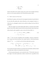
2.4
M ODELLING
THE
P OLARIZATION
AND
P HOTON E CHO
The model system is an electronic two-level system with T1 T2 , meaning the population relaxation time, T1 , is much longer than the dephasing time, T2 . A nearly impulsive
radiation field with a very short pulsewidth (FWHM of 5 fs) and low frequency (3000
cm−1 ) was used in the model calculation in order to reduce computer time.
The polarization was found directly by computing the expression in Eq 2.16 using
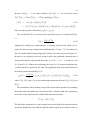
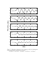
the program given in Appendix A. Polarization components for five frequency components within the inhomogeneous broadening bandwidth are given in Figure 2.3. The delay
between pulse one and two was fixed at 50 fs for these calculations, with pulse two occurring at t = 0. We note that the five polarization components remain out of phase until 50
fs, the time after pulse two which equals the delay between pulse one and pulse two. At
50 fs, all the polarization components are seen to be in phase, creating the photon echo.
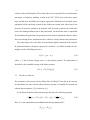
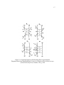
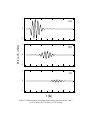
The photon echo was found by summing the calculated polarization components from
200 frequency components contributing to the inhomogeneous broadened line according
to the program given in Appendix B. Calculations of the photon echo illustrate the
behavior of the echo as the delay between pulses k1 and k2 = k3 is varied, as shown in
Figure 2.4. As expected, the photon echoes occur at a time interval after the arrival of k 2
equal to the delay between k1 and k2 . As the delay increases, the amplitude of the photon
echo signal decreases. When the change in amplitude is graphed with respect to delay
time, an exponential decay of e−t/T2 results.
20
1
(a)
0
-1
-25
0
25
50
75
0
25
50
75
0
25
50
75
0
25
50
75
0
25
50
75
1
(b)
P(t) (arb. units)
0
-1
-25
1
(c)
0
-1
-25
1
(d)
0
-1
-25
1
(e)
0
-1
-25
t (fs)
Figure 2.3: Polarization components for five frequencies within the inhomogeneous
broadening bandwidth, zero phonon line at 3000 cm−1 .
(a) 2500 cm−1 , (b) 2750 cm−1 , (c) 3000 cm−1 , (d) 3250 cm−1 , (e) 3500 cm−1
21
1
(a)
0
-1
P(t) (arb. units)
0
50
100
200
150
1
(b)
0
-1
0
50
100
200
150
1
(c)
0
-1
0
50
100
150
200
t (fs)
Figure 2.4: Photon echoes calculated at three delays between pulses 1 and 2.
(a) 25 fs delay, (b) 75 fs delay, (c) 125 fs delay
22
Calculations of the photon echo signal as a function of the delay τ between the pulses
will be presented and discussed at the end of Chapter Three.
2.5
R EFERENCES
[1] Marc D. Levenson, Introduction to Nonlinear Laser Spectroscopy, (Academic
Press, New York, 1982).
[2] Shaul Mukamel, Principles of Nonlinear Optical Spectroscopy, (Oxford University Press, London, 1995).
[3] L. E. Fried, S. Mukamel, Adv. Chem. Phys. LXXXIV, 435, (1993).
[4] Eugen Merzbacher, Quantum Mechanics: Second Edition, (John Wiley & Sons,
New York, 1970).
[5] Stig Stehnolm, Foundations of Laser Spectroscopy, (John Wiley & Sons, New
York, 1984).
[6] M. Joffre, Coherent Effects in Femtosecond Spectroscopy: A Simple Picture
Using the Bloch Equation in Claude Rulliére (Ed.), Femtosecond Laser Pulses,
(Springer, Berlin, 1998).
[7] T. K. Yee, T. K. Gustafson, Phys. Rev. A, 18, 1597, (1978).
[8] J.D. Jackson, Classical Electrodynamics, (John Wiley & Sons, New York, 1962).
[9] Robert W. Boyd, Nonlinear Optics, (Academic Press, Boston, 1992).
C HAPTER 3
E XPERIMENTAL U LTRAFAST D EGENERATE F OUR -WAVE M IXING
3.1
T HE L ASER S YSTEM
An actively modelocked Ti:Sapphire laser is used to generate ultrashort pulses on the order
of 70 femtoseconds. The system is composed of: (1) an intracavity doubled Nd:YVO 4
solid state pump laser, and (2) an actively modelocked ultrafast titanium sapphire laser
followed by an optional frequency doubler. Characterization equipment includes an autocorrelator for measuring the pulse width, and a rotating grating spectrometer for monitoring the bandwidth. Each component is described in detail below.
3.1.1
N D :YVO4 P UMP L ASER
The Nd:YVO4 laser (Spectra Physics Millennia [1]) is optically pumped by two fiber optic
bundles which propagate the output of two GaAlAs diode laser bars lasing at 809 nm.
Each diode laser bar is capable of 20 W power output but is operated at only 75% of the
maximum power output to increase longevity and to enable stabilization of the Nd:YVO 4
laser. Operating at less than full power allows for minor misalignment of the Nd:YVO 4
laser to be compensated for by increasing or decreasing the electric current to the diodes.
The usefulness of this feature was observed when the lenses focusing the diode emission
into the fiber optic bundles became misaligned, resulting in reduction of the pumping
efficiency. The attempts by the feedback system to correct the power deficiency resulted
in dramatic current increases recorded to the diodes and provided a clue as to the source
23
24
20,000
18,000
16,000
4
14,000
2
cm−1
12,000
S 3/2 4 F 7/2
4
H 9/2 F 5/2
4
F 3/2
4
I 15/2
4
I 13/2
4
I 11/2
4
I 9/2
Pump
Bands
10,000
8,000
6,000
4,000
2,000
0
Lasing
Transition
Figure 3.1: Four-Level Lasing System of the Nd3+ ion
of the problem. The increase in current was capable of counterracting the misalignment
problem until the misalignment became severe.
The neodymium yttrium vanadate (YVO4 :Nd
3+
) laser is operated in a continuous
working (CW) mode. YVO4 :Nd3+ is a four level laser as can be seen from Figure 3.1.
A four level system enables a population inversion to be maintained, thus allowing continuous working operation. Nd3+ has a strong absorption band at 860 nm, which is overlapped by the diode laser emission. The optically excited electrons rapidly nonradiatively
25
decay from the 4 S 3 , 4 F 7 , 2 H 9 , and 4 F 5 levels to the 4 F 3 level and radiatively decay to the
2
4
2
2
2
2
4
I 11 state, lasing at 1064 nm. From the I 11 state they relax rapidly to the 4 I 9 ground state.
2
2
2
4
The combination of the relatively long lifetime at the F 3 storage level (60 µs) and the
2
rapid relaxation to the ground level creates a population inversion and therefore an ideal
lasing transition.
The 1064 nm emission is intracavity doubled using a lithium triborate (Li 3 BO3 ) nonlinear mixing crystal to generate a 532 nm continuous wave emission at a power of 5 W;
it is this laser emission that is used to pump the Ti:Sapphire laser.
3.1.2
T I :S APPHIRE L ASER
The ultrashort pulse laser (Spectra Physics Tsunami[2]) uses a Ti3+ doped sapphire
(Al2 O3 ) crystal as its laser medium. The Ti3+ ions are strongly coupled to the vibrational
modes of the host resulting in broad emission bands. The absorption band extends from
400 nm to 650 nm, the peak occurring near 500 nm as shown in Figure 3.2. The emission
band extends from 600 nm to 1050 nm, but lasing only occurs to the red of 670 nm due
to overlap with the absorption band. Although the peak of the laser emission occurs at
790 nm, the laser has a tuning range from 690 nm to 1080 nm. The experiments described
in this thesis were performed using pulses with wavelength 790 nm which were then frequency doubled. A 3.66 m pathlength is created in an enclosure smaller than 1 m through
the use of a folded cavity. A prism is used to spectrally disperse the beam, allowing a
variable slit to be used to tune the bandwidth. Bandwidths smaller than 11 nm cause
significant pulse lengthening while bandwidths larger than 27 nm lead to instability of
the laser. After bandwidth selection, the beam is sent through a second prism to reverse
the spectral dispersion of the first prism. Modelocking of the laser is accomplished using
an acousto-optic modulator. The resulting pulses have a temporal width of nominally 70
femtoseconds with a repetition rate of 82 MHz, yielding an average power of ∼800 mW.
Though the energy of each pulse is very small, on the order of 10 −8 J, the peak power
26
Figure 3.2: Absorption and Emission Spectra of Al2 O3 :Ti3+
(From Ref. [2])
27
is high (∼140 kW) due to the short temporal width. The ultrafast laser emission is analyzed using a fast photo diode, a real time spectrometer, and an autocorrelator. The laser
emission can be frequency doubled to create ultraviolet light at 395 nm.
Laser power is monitored by a power meter placed at the output coupler. Usually
adjustments are made only to the prisms and tuning slit to obtain the highest power readings. Very low laser power and instability are corrected by adjusting the placement of the
internal steering mirrors of the laser.
A beam splitter directs a small portion of the pulsing output into a fast photodiode.
The readings of the photodiode are shown on an oscilloscope and reveal the stability of
the pulsetrain. If a strong and stable pulse is not consistently seen, then the Ti:Sapphire
laser should be optimized to increase both power and stability. Once optimized, the design
of the laser provides stable operation under consistent environmental conditions for over
the period of a day, and requires only prism and slit adjustments to maintain power and
stability beyond that time period.
3.1.3
P ULSEWIDTH M EASUREMENT
An indirect measurement of the pulsewidth is obtained using an autocorrelator (Spectra
Physics Model 409[3]). The autocorrelator splits the incoming beam and uses a rotating
block of fused silica placed in the path of both beams to create a variable difference
in the optical pathlength. The difference in pathlength ∆L of one beam is given by the
expression
q
∆L = 2d( n2 − sin2 θ − cos θ + 1 − n)
where d and n are the thickness and index of refraction of the block respectively. The
beams are aligned onto the rotating block at complementary angles, resulting in a difference in pathlength between the two given by
q
√
∆Lθ = 2d[( n2 − sin2 θ − cos θ) − ( n2 − cos2 θ − sin θ)]
28
As the block rotates, the beams travel in opposite directions, alternating between maximum and minimum pathlength distances: When one beam is at a maximum, the other is
at a minimum. When both beams are incident on the block at an angle of 45 ◦ , the two pathlengths are equal and the pulses are temporally overlapped. The beams are then focused
by a lens and spatially overlapped inside a frequency doubling crystal. The autocorrelator
signal is seen when the beams are both spatially and temporally overlapped within the
frequency doubling crystal. The autocorrelator signal is of the form
1
T →∞ T
C(τ ) = lim
Z
t0 +T
t0
x(t)x(t + τ )dt
where τ is the difference in temporal pathlengths and T is the time interval of the data
scan[4]. The signal is filtered by an ultraviolet band pass filter and directed into a photomultiplier tube housed within the autocorrelator. The resulting signal is viewed on an
oscilloscope. The fused silica block rotates 30 times per second, resulting in 60 signals
per second being sent to the oscilloscope. The pulsewidth of the autocorrelation signal is a
t
) laser pulse (where
function of the pulse shape, and the true FWHM ∆σ of the sech2 ( ∆Σ
∆Σ is the pulsewidth) is scaled by a factor of s=0.65 of the autocorrelation trace,
∆σ = s∆σ 0
where ∆σ 0 is the FWHM of the signal as shown on the oscilloscope.
A fixed delay of 2∆d0 n0 /c is introduced into one of the pathlengths by placing a calibrating etalon within the beampath in a position where the beam will travel through it
twice. The etalon has a thickness of ∆d0 and an index of refraction of n0 . The temporal
FWHM of a pulse ∆σ is found from the oscilloscope readings by the following calculation:
∆σ =
∆σ 0 2∆d0 n0
s
∆p
c
where ∆p is the distance between adjacent pulses as measured on the oscilloscope and
c is the speed of light. For the autocorrelator used in this work, 2∆d 0 n0 /c = 310 fs.
29
An example of the autocorrelation trace with and without the etalon delay is given in
Figure 3.3.
3.1.4
BANDWIDTH C HARACTERIZATION
The spectral bandwidth of the ultrashort pulses is measured by directing a small fraction of
the laser emission into a laser spectrum analyzer (IST-REES E200 series). This instrument
enables the spectrum of the laser to be monitored in real time, facilitating optimization of
the laser. A diffraction grating inside the instrument spins at a rate of 18 revolutions per
second, continually scanning the spectrum. The output is viewed on an oscilloscope in real
time. The bandwidth is measured by calculating the FWHM of the spectrum displayed on
the oscilloscope to an accuracy of ±0.3 nm as shown in Figure 3.4. The laser is adjusted
so that the bandwidth is in the range of 12 to 23 nm.
3.2
E XPERIMENTAL C ONSIDERATIONS
3.2.1
Y2 S I O5 :C E3+
6
Y2 SiO5 is a monoclinic crystal that belongs to the C2h
space group[5]. Each unit cell
contains eight molecules, and the Ce3+ cations occupy two inequivalent crystallographic
sites within the cell. It is not known which site is preferred by the cations, which are
considered to be distributed randomly in the host.
Trivalent cerium has the electronic configuration [Xe]4f1 . The energy gap between the
ground state and the lowest 5d orbital is large, ranging from 20,000-35,000 cm −1 . The
ground state in free radical form is split by spin-orbit effects. When surrounded by the
crystal field of a host, the two levels are split further. Excitation occurs from the 4f ground
level to the 5d level. An energy level diagram is given in Figure 3.5.
Y2 SiO5 :Ce3+ is a rapid response blue phosphor[6][7][8] having a decay to 10% time
of 120 ns and is mainly used for electron detection in scientific instruments such as mass
Normalized Autocorrelation Signal
30
∆ t=310 fs
1
0.5
0
∆σ ’ = 110 fs
0
1
2
3
4
5
6
t (arbitrary units)
Figure 3.3: Autocorrelation trace showing a delay of 310 fs between pulses.
Unscaled autocorrelator signal pulsewidth = 110 fs. Actual laser pulsewidth = 71 fs
7
Normalized intensity (arb. units)
31
1
∆λ =13.0 nm
0.5
0
770
775
780
785
790
795
800
Wavelength (nm)
Figure 3.4: Bandwidth Characterization
805
810
32
Energy
(x 1000 cm −1)
30
5d
5
2
F 7/2
2
0
F 5/2
4f
Figure 3.5: Electronic energy levels for trivalent Ce3+
33
spectrometers and electron microscopes. Its resistance to ultraviolet and fluid damage also
makes it useful in high energy scientific instruments[9].
The sample used in this research was a small plate that was optically polished on the
two largest faces using 5 µm diamond grit. The dimensions of the polished sample were
2.5 mm × 1.5 mm × 0.1 mm.
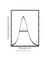
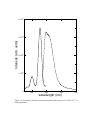
The excitation and emission spectra for the sample were taken using a spectrofluorometer system (Jobin Yvon-SPEX Fluoromax-2) at room temperature and are given in
Figure 3.6. Peak excitation occurs at 350 nm, and peak emission at 400 nm. Emission is
broadband, extending from 400 to 420 nm. The shift between the excitation and emission
spectrum is called the Stokes shift and is a measure of the electron lattice coupling.
3.2.2
I NTRODUCTION
TO
N ONLINEAR S PECTROSCOPY
AND
D EGENERATE F OUR -
WAVE M IXING
One of the major experimental techniques that takes advantage of the third order susceptibility is four-wave mixing (FWM)[12][13]. This technique which can be used to measure
both population decay and electronic dephasing includes a variety of nonlinear optical
experiments such as photon echoes.
Three laser pulses having wave-vectors k1 , k2 , and k3 interact at the sample to produce
a fourth signal with a wave-vector in the k4 = k1 ± k2 ± k3 direction. The frequencies of
the three pulses add with the same sign as the wave vectors. The three interacting waves
therefore generate a fourth wave with frequency ω4 = ω1 ± ω2 ± ω3 in the direction
specified by the wave vectors.
There are several variations of the basic FWM experiment. FWM signals can be
described in either the frequency domain or time domain. For ultrashort pulses which
have a broad frequency spectrum, the time domain description is more appropriate. In
time domain FWM, the behavior of the third pulse as the delay time between the first two
pulses is varied provides us with information about population decay time, or dephasing
34
5
8×10
5
Intensity (arb. units)
6×10
5
4×10
5
2×10
0
300
400
500
600
wavelength (nm)
Figure 3.6: Excitation (solid line) and emission (dotted line) spectra for Y 2 SiO5 :Ce3+ at
room temperature.
35
time. By choosing the polarization combination of the incoming pulses, it is possible to
measure different components of the nonlinear susceptibility tensor, and create different
types of electronic polarizations within the material. In addition, the direction of the signal
chosen for observation can be varied according to the characteristics of the system. The
diffracted signal can be measured in the forward direction (transmission geometry) or in
the backward direction (reflection geometry). The reflection geometry is valuable for thin
films where the absorption of the substrate would make the forward signal weak, and thus
difficult to measure[12]. By varying the propagation directions of the incoming beams,
different experiments can be performed. For example, having two pump beams approach
the sample from opposite sides, followed by a third beam incident on the medium in a
different direction, results in the phase conjugate of the third beam. When the phase conjugated beam passes through the same aberrating medium the third wave passed through,
aberrations in the third beam are removed. In this type of experiment, the two pump beams
can be used to remove aberrations of waves passing through an external medium[11].
When all three pulses originate from the same laser, then they are of equal frequencies,
leading to the simplest type of FWM, termed degenerate four-wave mixing (DFWM).
In addition, k2 and k3 can originate from the same beam, simplifying the geometry to
two-beam DFWM. The resulting signal wave-vector is 2k2 − k1 and the resulting signal
frequency is 2ω2 − ω1 = ω1 (see Figure 3.7). Two-beam DFWM is the technique used
in this thesis. In this experiment the three pulses can be considered to interact in the
following way: The first pulse, k1 , creates an electronic superposition state, creating a
time varying polarization. A second pulse, k2 , arrives at the sample after a fixed delay
time, and modulates the polarization created by k1 . This polarization then radiates the
signal field. If the delay time between the first and second pulse is less than the time
required for the sample to lose its phase memory due to system-bath interactions, termed
the dephasing time, no nonlinear signal will be observed.
36
2k2 − k1
k1
k2
Sample
k1
k2
k3
2 k 1− k 2
Figure 3.7: Two-Beam Degenerate Four-Wave Mixing
A particularly simple form of DFWM which is often a useful model for interpreting
the experiment is the transient grating. Two beams incident on the sample at an angle with
respect to each other cause an interference patterns. Bright areas where the two beams
interfere constructively will cause electronic transitions to a resonant excited state. Dark
areas where the two beams interfere destructively will result in the electronic population
remaining in the ground state, resulting in a population grating. The third pulse, k 2 again,
then arrives at the sample and is diffracted by the population grating. The signal generated
by the third pulse provides information on the population lifetimes.
3.2.3
DFWM E XPERIMENTAL S ET-U P
A schematic of the experimental setup is shown in Figure 3.8. The output of the
Ti:Sapphire laser is divided by a 50% beamsplitter into two paths. One path contains
a high precision translation stage (Newport UTMPP.1), allowing for a delay in the optical
path of up to 4 inches with a precision of 0.1 µm. An iris is placed immediately in front of
37
M1
Nd:YVO4 Laser
Diode Laser
Optical Fibers
Ti:Sapphire
M3
Laser
BS2
M2
BS3
BS1
Autocorrelator
FM1
M5
Fast Photodiode
Spectrum
Analyzer
Optional
Frequency
Doubler
M6
M7
I2
k1
I1
M4
FM2
M8 M9
I3
BS4
k2
M10
Optical
Chopper
focusing
lens
Retro reflector
Sample
Translation Stage
2 k1 − k2
focusing
lens
2 k2 − k1
Photodiode on
translation stage
Lock−In
Amplifier
Figure 3.8: Experimental Set-Up for Degenerate Four-Wave Mixing
BS=beam splitter, FM=flip mirror, I=Iris, M=mirror
38
the beam splitter. In addition, a second and third iris are placed at the end of each pathway,
immediately in front of the focusing lens. Because even a small change in pathlength of
one path can drastically effect the temporal overlap area of 70 fs pulses, the use of these
irises enables the beam paths to be reproduced from day to day, counteracting the effects
of mirror drift and changes resulting from laser alignment.
Before focusing, the two beams are “chopped” at different frequencies by a optical
chopper wheel (Stanford Research Systems Model SRS540). The chopper wheel contains
an inner and outer set of blades, each set having a different number of apertures. One beam
is passed through each set of blades, ensuring a difference in the chopping frequencies of
the two beams. The chopper ensures that only a signal generated by a combination of the
two frequencies, and thus the two beams, is detected by the lock-in amplifier (Stanford
Research Systems Model SR380). Any scattering from either of the beams is chopped
only at the frequency of the source beam and is therefore discriminated against. Only
a signal resulting from the interaction of the two beams will be modulated at the sum
frequency, and therefore amplified. The two beams are then focused into the sample using
a short focal length, 3 cm, convex lens. Spatial overlap in the sample is achieved by placing
one steering mirror in each path after the third iris and before the focusing lens. The two
beams are aligned parallel over a distance of approximately 5 m, ensuring spatial overlap
when focused into the sample. Temporal overlap is most quickly achieved by using a
mirror to divert the aligned and focused beams into an Li3 BO3 second harmonic crystal,
and adjusting the placement of the translation stage until the two focused beams produce
a single beam of frequency doubled light visible between them. Once temporal overlap is
achieved, the beams are again directed into the sample.
3.2.4
D ETECTION
After the sample, all pump and signal pulses are collimated using a 7 cm focal length
convex lens. A fast photo diode (New Focus Model 1621) having a detection surface of
39
1 mm2 is placed on a translation stage, allowing it to be moved from one signal pulse to
the other to select the signal for analysis. Laser scatter is reduced using an aperture.
3.2.5
DATA ACQUISITION P ROGRAM
The three motion stages and the lock-in amplifier were interfaced through the General
Purpose Interface Bus (GPIB) and controlled by a microcomputer. The GPIB interface
allows up to fifteen devices to communicate through a central controller, regardless of the
individual manufacturer or device language. A program was written in Visual Basic to
simultaneously control the motion stages within the experimental set-up and data collection by the lock-in amplifier. This program provides a graphical user interface to enable
the user to set the parameters for each experimental scan, as listed below.
Motion Stages
• zero point, or home position
• initial position of scan
• starting and stopping acceleration
• starting and stopping velocity
• velocity during motion
• size of each step
• resolution of each step
• time allotted for settling after each step
• total travel length, in absolute or relative distance
Lock-In Amplifier
• form of output, (r, θ) or (x,y)
• triggering function
40
• internal or external source for triggering
• default values
• number of data points collected and averaged per step
Data Display
• maximum and minimum values of each axis
• total data acquisition or portion of data acquisition displayed
• step unit desired
• total number of scans taken
The results were plotted in real time as the data was being taken, allowing the user to
abort a scan, if necessary. After data was acquired, the user could choose to limit the data
shown on the screen, and “zoom-in” on regions of interest. The values of the axes could
be varied both before and after data was taken. Data was saved in files named by the user.
This program is given in Appendix C at the end of this thesis.
3.3
3.3.1
R ESULTS
AND
D ISCUSSION
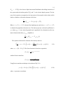
E XPERIMENTAL R ESULTS
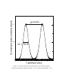
The intensity of the four-wave mixing signals in the 2k1 − k2 and 2k2 − k1 directions
was measured as a function of the delay time τ between the pulse with wave-vector k 1
and the pulse with wave-vector k2 . For a sample with a fast dephasing time relative to the
pulsewidth, the dephasing time of the sample can be studied by examining the shift
between the peaks of the 2k1 − k2 and 2k2 − k1 signals. In the initial experiments, the
four-wave mixing signals exhibited various peak shifts with no discernible pattern. It was
subsequently discovered that this effect was due to backlash in the translation stage
controlling the pathlength of k2 . After compensating for this problem, Carl Liebig
Normalized DFWM Signal Intensity
41
1
0.5
0
-500
0
500
Delay Time (fs)
Figure 3.9: Two beam degenerate four-wave mixing signals measured on Y 2 SiO5 :Ce3+ at
395 nm. Filled circles are 2k2 − k1 signal. Open circles are 2k1 − k2 signal. Data courtesy
of Carl Liebig.
42
gathered data on the sample which illustrated no shift between the peaks as shown in
Figure 3.9.
3.3.2
M ODELLING
THE
R ESULTS
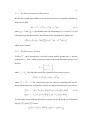
Four-wave mixing signals for the model system described in Chapter Two were
calculated from the program given in Appendix D.
The shape of the four-wave mixing signals calculated with dephasing times of 0.01 fs
and 2.5 fs (0.002×pulsewidth and 0.5×pulsewidth respectively) are very similar
(although with a slight shift), illustrating the difficulty in determining an accurate
dephasing time when T2 is much shorter than the laser pulsewidth. When the dephasing
time is equal to or longer than the pulsewidth, as shown in the echo signals calculated
with dephasing times of 5.0 fs and 10.0 fs (equal to and twice the laser pulsewidth
respectively) a noticeable asymmetry can be seen in the signal. Dephasing times which
are long relative to the external pulsewidth would give a signal with an exponential tail
with characteristic time T2 and would exhibit a peak shifted significantly from zero.
Dephasing times which are short relative to the external pulsewidth would give a signal
shape similar to the external radiation pulseshape obtained by an autocorrelation
measurement. Both the 0.01 fs and 2.5 fs dephasing time calculations and the
experimental data (see Figure 3.9) exhibit minimal shift and the pulseshapes of both are
identical to that of the laser as shown in Figure 3.3. It is therefore concluded that the
dephasing time of Y2 SiO5 :Ce3+ is significantly shorter than the laser pulsewidth of 70 fs.
3.4
R EFERENCES
[1] Millennia Diode-pumped, CW Visible Laser User’s Manual, Instruction Manual,
(Spectra-Physics, Mountain View, 1997).
43
1
(a)
Normalized DFWM Signal Intensity
0.5
0
-25
1
0
25
50
(b)
0.5
0
-25
1
0
25
50
(c)
0.5
0
-25
1
0
25
50
(d)
0.5
0
-25
0
25
50
Delay Time (fs)
Figure 3.10: Echo signals as a function of delay calculated at various dephasing times
with a laser FWHM pulse of 5 fs.
(a) T2 = 0.01 fs, (b) T2 = 2.5 fs, (c) T2 = 5.0 fs, (d) T2 = 10.0 fs
44
[2] Tsunami Mode-Locked Ti:Sapphire Laser User’s Manual, Instruction Manual,
(Spectra-Physics, Mountain View, 1995).
[3] Model 409 Autocorrelator User’s Manual, Instruction Manual, (Spectra-Physics,
Mountain View, 1995).
[4] Gregory H. Wannier, Statistical Physics, (John Wiley & Sons, Inc., New York,
1966).
[5] Rufus L. Cone, Phys. Rev. B, 52,6 (1995).
[6] P. J. Marsh, J. Silver, A. Vecht, A Newport, J. Lumin., 97, 229, (2002).
[7] S. H. Shin, D. Y. Jeon, K. S. Suh, Jap. J. App. Phys. I, 40, 4715, (2001).
[8] Y. Liu, C. N. Xu, K. Nonaka, H. Tateyama, J. Mat. Sci., 36, 4361, (2001).
[9] Phospor/Scintillator Data Sheet 24: yttrium silicate-cerium doped, (Applied
Scintillation Technologies, London, 2000).
[10] Madis Raukas, Ph.D. dissertation Luminescence Efficiency and Electronic
Properties of Cerium Doped Insulating Oxides, (1997).
[11] Robert W. Boyd, Nonlinear Optics, (Academic Press, Boston, 1992).
[12] Jagdeep Shah, Springer Series in Solid-State Sciences 115: Ultrafast
Spectroscopy of Semiconductors and Semiconductor Nanostructures,
(Springer-Verlag, Berlin, 1996).
[13] A. M. Weiner, S. De Silvestri, E. P. Ippen, J. Opt. Soc. Am. B, 2, 654, (1985).
C HAPTER 4
C ONCLUSIONS
The spectroscopic properties of Y2 SiO5 :Ce3+ were investigated at room temperature.
The sample was found to have a peak excitation at 350 nm and a broadband emission
between 400 and 420 nm. An ultrafast two beam degenerate four-wave mixing
experiment was set up and utilized to establish an lower limit on the dephasing time of
Y2 SiO5 :Ce3+ at room temperature at an excitation frequency of 395 nm. For these
experiments a Ti:sapphire laser was used to produce 790 nm pulses at a repetition rate of
82 MHz. Laser pulses were characterized using a rotating grating spectrometer to
determine the spectral bandwidth and using a rotating block autocorrelator to determine
the temporal pulsewidth. The laser pulses had a temporal pulsewidth of 60 to 80 fs and a
spectral bandwidth ranging from 12 to 23 nm, depending on the requirements of the
experiment; these pulses were then frequency doubled to 395 nm.
Experimental data using a laser pulsewidth of 70 fs revealed no shift between the
2k2 − k1 and 2k1 − k2 four-wave mixing signal peaks. In addition, the experimentally
obtained photon echo signals showed no obvious asymmetry. The experimental results
are consistent with calculations performed on a model system having a dephasing time
significantly shorter than the laser pulsewidth; as a result the dephasing time of
Y2 SiO5 :Ce3+ is concluded to be significantly shorter than the pulsewidth of the laser, i.e.
70fs. Since the dephasing rate T2−1 provides a measure of the coupling of the electronic
system to the bath, this result indicates that the electron-lattice coupling is strong in this
system as is expected from the large Stokes shift.
45
A PPENDIX A
C ALCULATING
THE
P OLARIZATION C OMPONENTS
c
c
c
c
c
c
c
c
c
c
program joffres_polarization
implicit none
THIS PROGRAM IS A VARIATION OF MAIN PROGRAM
BJOFFRE.F AND CALCULATES THE POLARIZATION
FOR ONE FREQUENCY COMPONENT OF THE INHOMOGENEOUS
BROADENING AT A FIXED TAUPRIME DELAY VALUE BETWEEN
PULSE 1 AND PULSE 2. NOTES FOR POLARIZATION
PROGRAM WRITTEN IN ALL CAPS. THIS PROGRAM IS A MODEL
SO WEG IS NOT THE TRUE TRANSITION FREQUENCY
OF CERIUM DOPED YTTRIUM SILICATE. THE PROGRAM
MODELS POLARIZATIONS WHICH OCCUR AT AND SLIGHTLY OFF
THE TRANSITION FREQUENCY.
c
c
c
c
c
c
c
c
c
c
c
c
c
c
c
c
c
c
c
PARAMETERS FROM PARAMETER FILE:
isteps=number of divisions to create in interval
mystop-mystart when calculating values of
density operators and P**2(t)
mystart=time in fs at which your external radiation
pulses first hit the sample, time at which
Greens functions begin taking effect, must
be greater than or equal to zero
mystop= time at which external radiation stops
hitting sample, Greens functions no longer
have an effect in sample tau=delay between
external pulses 2 and 3,should be zero
w1=frequency of external radiation for all three
pulses,in wavenumbers
weg=zero phonon line of first order signal from
sample,in wavenumbers
hbar, k Planck,Boltzmann constant
t1=T1, the eigenstate decay rate, relaxation of
density operator
46
47
c
diagonal matrix elements
c t2=T2 dephasing rate, relaxation of density operator
c
off-diagonal matrix elements
c fwhm=fwhm of external radiation pulse in fs
integer nmax,i,imax
real pi,sigma
parameter (nmax=524288,pi=3.14159)
$
$
$
$
$
real t,signalmax
,isteps,mystart,mystop,w1,weg,tau,tauprime,hbar,k
,rp3(nmax),ip3(nmax)
,rp2(nmax),ip2(nmax),rp1(nmax),ip1(nmax)
,rgeg(nmax),igeg(nmax),tsteps,t1,t2,fwhm
,gegr,gegi,geer,geei
$
$
$
$
$
$
$
real rconv(nmax),iconv(nmax)
,invrconv(nmax),inviconv(nmax)
,invrgeg(nmax),invigeg(nmax)
,rgee(nmax),igee(nmax),signal(nmax)
,re1(nmax),ie1(nmax),invre1(nmax)
,invie1(nmax),rfunc(nmax),ifunc(nmax)
,re2(nmax),ie2(nmax),re3(nmax),ie3(nmax)
,rdipge,idipge,elec
$
$
complex e1(nmax),e2(nmax),e3(nmax),inve1(nmax)
,p1inv(nmax),polar(nmax)
,conv,p3(nmax),geg,gee,p2(nmax),p1(nmax),dipge
common /values/ hbar,weg,t1,t2,mystop
common /times/ tsteps,tau,tauprime
common /elecvals/ w1,sigma
character*16 fname
rdipge=1.0
idipge=0.0
dipge=cmplx(rdipge,idipge)
$
$
c
read (*,*) isteps,mystart,mystop,tau
,w1,weg,hbar,k
,t1,t2,fwhm
redefine wavenumber input into correct units
48
c
c
of frequency. calcs are done with frequencies
in units of 1/ fs (1e15/s)
w1=2*pi*3e8*w1*1e-13
weg=2*pi*3e8*weg*1e-13
c sigma=pulsewidth of external radiation field in fs,
c fwhm/1.76
sigma=fwhm/1.76
c GF exists only for 1st half of total increments, so
c imax is set at .5 of total isteps
imax=int((isteps+1)/2)
c
c
c
c
c
c
FIRST PULSE, E1, OCCURS AT -50FS COMPARED TO E2 AND E3
FOR POLARIZATION CALC. FOR THE POLARIZATION CALC
THE SECOND PULSE OCCURS AT A DELAY OF 50 FS
POLARIZATION WILL BEGIN FROM POINT WHEN
SECOND AND THIRD PULSE SET UP AND DIFFRACT THROUGH
TRANSIENT GRATING.
tauprime= 50
tsteps=(mystop-mystart)/isteps
c establish initial arrays from which all convolutions
c will be composed
i=1
do i=1,nmax
c
c
c
c
c
c
The characteristics of how convolutions are programmed
require that the response functions are calculated so
G(i=1) is evaluated at t=0 and elec funcs are calculated
so E(i=1) is evaluated at mystart. The GF(t>0) are
convoluted, however, with the E(t<0). Do not wait for
t>0 to begin convoluting GF with E(t).
t=mystart+(i-1)*tsteps
if (i.le.(isteps+1)) then
c E1(T) IS CHANGED TO E1(T+TAUPRIME), CAUSING THE TIME AT
49
c WHICH E1 OCCURS TO BE SHIFTED TO THE LEFT (EARLIER)
c BY TAUPRIME SO THAT E2, E3, AND GF WILL BE CALCULATED
c FROM T=0.
e1(i)=elec(t+tauprime)
$
*cmplx(cos(w1*(t+tauprime*0.)),
$ -sin(w1*(t+tauprime*0.)))
else
e1(i)=0.
endif
inve1(i)=conjg(e1(i))
invre1(i)=real(inve1(i))
invie1(i)=imag(inve1(i))
enddo
c
c
c
c
c
c
c
c
c
Green functions must be calculated for t>0 only, but
convoluted with E(t<0) values determined by value of
mystart. To ensure that elements E(t)(i) begin at
mystart, and elements G(i) begin at t=0, separate loop
is needed to redefine t for array elements i when
determining the Green function. GF do not care about
time values. they care only that they are divided into
the same number of intervals as the pulses, regardless
of time values.
i=1
do i=1,nmax
t=(i-1)*tsteps
if (i.le.imax) then
rgeg(i)=gegr(t)
igeg(i)=gegi(t)
rgee(i)=geer(t)
igee(i)=geei(t)
else
rgeg(i)=0.
igeg(i)=0.
rgee(i)=0.
igee(i)=0.
endif
invrgeg(i)=-real(conjg(cmplx(rgeg(i)
$ ,igeg(i))))
invigeg(i)=-imag(conjg(cmplx(rgeg(i)
$ ,igeg(i))))
enddo
50
c p1=invgeg*inve1 in freq space, FT[G(t)]*FT[E(t)]=
c G(w)*E(w)
call fft(invrgeg,invigeg,nmax,nmax,nmax,1)
call fft(invre1,invie1,nmax,nmax,nmax,1)
c FT[G(t)]*FT[E1(t)]=G(w)*E(w)
i=1
$
$
do i=1,nmax
invrconv(i)=real(cmplx(invrgeg(i),invigeg(i))*
cmplx(invre1(i),invie1(i)))
inviconv(i)=imag(cmplx(invrgeg(i),invigeg(i))*
cmplx(invre1(i),invie1(i)))
end do
c p1(t) obtained from FT[FT[Ginv(t)]*FT[Einv(t)]]
call fft(invrconv,inviconv,nmax,nmax,nmax,-1)
c E*FT[FT[Ginv(t)]*FT[Einv(t)]]=E*p1
i=1
do i=1,nmax
t=mystart+(i-1)*tsteps
if (i.le.(isteps+1)) then
c E2 CALCULATED AT T, A DELAY OF TAUPRIME LATER THAN E1.
e2(i)=elec(t)*
$ cmplx(cos(w1*t),
$
-sin(w1*t))
else
e2(i)=0.
endif
p1(i)=e2(i)*cmplx(invrconv(i),inviconv(i))
rp1(i)=real(p1(i))
ip1(i)=imag(p1(i))
end do
c find FT[E2(t)*p1(t)] and FT[G(t)]
call fft(rp1,ip1,nmax,nmax,nmax,1)
call fft(rgee,igee,nmax,nmax,nmax,1)
51
i=1
do i=1,nmax
rconv(i)=real(cmplx(rgee(i),igee(i))*
$
cmplx(rp1(i),ip1(i)))
iconv(i)=imag(cmplx(rgee(i),igee(i))*
$
cmplx(rp1(i),ip1(i)))
enddo
c FT[FT[G(t)]*FT[E(2)(t) * p1(t)]]
call fft(rconv,iconv,nmax,nmax,nmax,-1)
do i=1,nmax
enddo
i=1
do i=1,nmax
t=mystart+(i-1)*tsteps
if (i.le.(isteps+1)) then
c E3 BEGINS AT T, A DELAY OF TAUPRIME LATER THAN E1.
e3(i)=elec(t)*
$ cmplx(cos(w1*t),
$
-sin(w1*t))
else
e3(i)=0.
endif
p2(i)=e3(i)*cmplx(invrconv(i),inviconv(i))
rp2(i)=real(p2(i))
ip2(i)=imag(p2(i))
enddo
c p3=FT[G(t)]*FT[conv(t)].
c beginning of program.
Geg calculated in the
call fft(rp2,ip2,nmax,nmax,nmax,1)
call fft(rgeg,igeg,nmax,nmax,nmax,1)
i=1
$
$
i=1
do i=1,nmax
rconv(i)=real(cmplx(rgeg(i),igeg(i))*cmplx(
rp2(i),ip2(i)))
iconv(i)=imag(cmplx(rgeg(i),igeg(i))*cmplx(
rp2(i),ip2(i)))
enddo
call fft(rconv,iconv,nmax,nmax,nmax,-1)
52
do i=1,nmax
p3(i)=(-1)*cmplx(rconv(i),iconv(i))
c third order polarization=V(ge)*p3(eg)+
c invV(ge)*invp3(eg)=2Real(V(ge)p3(eg))
polar(i)=2*real(dipge*p3(i))
enddo
c THIS LOOP IS LIMITED TO RECORDING THE VALUES OF
c POLARIZATION (OR p3) FROM TIME VALUES OF -20 TO 150.
open(unit=88,file=’polarization.paw’)
do i=(-20-mystart)/tsteps+1,
$ (150-mystart)/tsteps+1
t=mystart+(i-1)*tsteps
write(88,*) t,real(p3(i))
enddo
close(88)
end
complex function gee(t)
implicit none
c green function in time domain
real hbar,gammaee,t,igee,rgee,weg,t1,t2,mystop
common /values/ hbar,weg,t1,t2,mystop
gammaee=1/t1
if (t.ge.0) then
gee=cmplx(0.0,exp(-gammaee*t)/hbar)
else
gee=cmplx(0.0,0.0)
endif
return
end
real function geer(t)
implicit none
real t
complex gee
if (t.lt.0) then
geer=0
else
53
geer=real(gee(t))
endif
return
end
real function geei(t)
c gee has only imaginary parts
implicit none
real t
complex gee
if (t.lt.0) then
geei=0
else
geei=imag(gee(t))
endif
return
end
complex function geg(t)
implicit none
c green function in time domain
real hbar,t,weg,gammaeg,t1,t2,mystop
common /values/ hbar,weg,t1,t2,mystop
gammaeg=1/t2
if (t.ge.0) then
geg=exp(-gammaeg*t)*cmplx(sin(weg*t),cos
$
(weg*t))/hbar
else
geg=cmplx(0.0,0.0)
endif
return
end
real function gegr(t)
implicit none
complex geg
real t
if (t.lt.0) then
gegr=0
else
gegr=real(geg(t))
endif
return
54
end
real function gegi(t)
implicit none
complex geg
real t
if (t.lt.0) then
gegi=0
else
gegi=imag(geg(t))
endif
return
end
real function elec(t)
implicit none
c real amplitude expression of electric field,
c E(t)=elec(t)eˆ(-iwt)
real t,tsteps,sigma,w1,sech,tau,tauprime
common /times/ tsteps,tau,tauprime
common /elecvals/ w1,sigma
elec=sech(t/sigma)
return
end
real function sech(t)
implicit none
real t
sech=2/(exp(t)+exp(-t))
return
end
A PPENDIX B
C ALCULATING
THE
P HOTON E CHO
c
c
c
c
c
c
c
c
c
c
program joffres_photonecho
implicit none
Variation of main program bjoffre.f.
Uses fast fourier transform method by Joffre
to calculate photon echo signal at a fixed
delay between pulses 1 and 2. Polarization
signals are calculated for frequencies within
the inhomogeneous broadening of the material.
The polarization signals are then added together
to generate a photon echo occuring at a time
after the 3rd pulse equal to the delay between
pulses 1 and 2.
c
c
c
c
c
c
c
c
c
c
c
c
c
c
c
c
c
c
c
PARAMETERS FROM PARAMETER FILE:
isteps=number of divisions to create in interval
mystop-mystart when calculating values of
density operators and P**2(t). Must be an integer.
mystart=time in fs at which your external radiation
pulses first hit the sample, time at which
Greens functions begin taking effect, must
be greater than or equal to zero
mystop= time at which external radiation stops hitting
sample, Greens functions no longer have an
effect in sample
tauprime=fixed delay between pulses 1 and 2.
tau=delay between ext pulses 2 and 3,should be zero
weg0=zero phonon line for transition freq in sample
w1=frequency of external radiation pulse
hbar, k Planck,Boltzmann constant
t1=T1, the eigenstate decay rate, relaxation of
density operator diagonal matrix elements
t2=T2 dephasing rate, relaxation of density operator
55
56
c off-diagonal matrix elements
c fwhm=full width half max time length of pulse of
c external radiation in fs
c minc=number of frequencies to include in the
c inhomogeneous broadening
integer nmax,i,m,minc,isteps
real pi,sigma,imax
parameter (nmax=524288,pi=3.14159)
$
$
$
$
$
$
real t,signalmax,wegmi,wegmf,deltaw,weight
,mystart,mystop,w1,weg,weg0,tau,tauprime,
hbar,k
,rp3(nmax),ip3(nmax)
,rp2(nmax),ip2(nmax),rp1(nmax),ip1(nmax)
,rgeg(nmax),igeg(nmax),tsteps,t1,t2,fwhm
,gegr,gegi,geer,geei,photonecho(nmax)
$
$
$
$
$
$
$
real rconv(nmax),iconv(nmax)
,invrconv(nmax),inviconv(nmax)
,invrgeg(nmax),invigeg(nmax)
,rgee(nmax),igee(nmax),signal(nmax)
,re1(nmax),ie1(nmax),invre1(nmax)
,invie1(nmax),rfunc(nmax),ifunc(nmax)
,re2(nmax),ie2(nmax),re3(nmax),ie3(nmax)
,rdipge,idipge,elec
$
$
complex e1(nmax),e2(nmax),e3(nmax),inve1(nmax)
,p1inv(nmax),polar(nmax),rhototal(nmax)
,conv,p3(nmax),geg,gee,p2(nmax),p1(nmax),dipge
common /values/ hbar,weg,t1,t2,mystop
common /times/ tsteps,tau,tauprime
common /elecvals/ w1,sigma
character*16 fname
rdipge=1.0
idipge=0.0
dipge=cmplx(rdipge,idipge)
$
read (*,*) isteps,mystart,mystop,tauprime,tau
,w1,weg0,hbar,k,t1,t2,fwhm,minc
57
c sigma=pulsewidth of external radiation field in fs
c sigma=fwhm/1.76 in units of param file
sigma=fwhm/1.76
c
c
c
c
c
redefine wavenumber input into correct units of
frequency calcs are done with frequencies in units
of 1/ fs (1e15/s) wegmi (wegmf) is the initial
(final) frequency from which inhomogeneous
broadening is calculated.
w1=2*pi*3e8*w1*1e-13
weg0=2*pi*3e8*weg0*1e-13
wegmi=weg0-2*pi*3e8*800*1e-13
wegmf=weg0+2*pi*3e8*800*1e-13
deltaw=(wegmf-wegmi)/minc
c loop over i before beginning m loop to initialize
c each element of the total density matrix and photon
c echo signal.
do i=1,isteps
photonecho(i)=0.0
rhototal(i)=0.0
enddo
c
c
c
c
c
loop over different frequency contributions weg to
the inhomogeneous broadening bandwidth. Weighting
factor weight will be multiplied to each frequency’s
contribution to the density matrix element for each
value of real time.
do m=1,minc+1
weg=0.0
weg=wegmi+(m-1)*deltaw
weight=exp(-((weg0-weg)/
$ (2*pi*3e8*500*1e-13))**2)
tsteps=(mystop-mystart)/isteps
c establish initial arrays from which all convolutions
c will be composed
58
i=1
do i=1,isteps
c
c
c
c
c
c
The characteristics of how convolutions are programmed
require that the response functions are calculated so
G(i=1) is evaluated at t=0 and elec funcs are calculated
so E(i=1) is evaluated at mystart. The GF(t>0) are
convoluted, however, with the E(t<0). Do not wait for
t>0 to begin convoluting GF with E(t).
c
c
c
c
e1 is calculated at e1(t+tauprime), meaning e1 will come
tauprime fs before pulses e2 and e3. e2 and e3 will start
at 0. The photon echo will occur tauprime fs after e2 and
e3 have hit the sample.
$
t=mystart+(i-1)*tsteps
if (i.le.(isteps+1)) then
e1(i)=elec(t+tauprime)*cmplx(
cos(w1*t),-sin(w1*t))
else
e1(i)=0.
endif
inve1(i)=conjg(e1(i))
invre1(i)=real(inve1(i))
invie1(i)=imag(inve1(i))
enddo
c
c
c
c
c
c
Green functions must be calculated for t>0 only, but
convoluted with E(t<0) values determined by value of
mystart. To ensure that elements E(t)(i) begin at
mystart, and elements G(i) begin at t=0, separate
loop is needed to redefine t for array elements i
when determining the Green function.
c GF exists only for 1st half of total increments, so
c imax is set at .5 of total isteps
imax=int((isteps+1)/2)
i=1
do i=1,isteps
t=(i-1)*tsteps
if (i.le.imax) then
rgeg(i)=gegr(t)
59
igeg(i)=gegi(t)
rgee(i)=geer(t)
igee(i)=geei(t)
else
rgeg(i)=0.
igeg(i)=0.
rgee(i)=0.
igee(i)=0.
endif
invrgeg(i)=real(conjg(cmplx(rgeg(i),igeg(i))))
invigeg(i)=imag(conjg(cmplx(rgeg(i),igeg(i))))
enddo
c p1=invgeg*inve1 in freq space, FT[G(t)]*FT[E(t)]=G(w)*E(w)
call fft(invrgeg,invigeg,isteps,isteps,isteps,1)
call fft(invre1,invie1,isteps,isteps,isteps,1)
c FT[G(t)]*FT[E1(t)]=G(w)*E(w)
i=1
$
$
do i=1,isteps
invrconv(i)=real(cmplx(invrgeg(i),invigeg(i))*
cmplx(invre1(i),invie1(i)))
inviconv(i)=imag(cmplx(invrgeg(i),invigeg(i))*
cmplx(invre1(i),invie1(i)))
end do
c p1(t) obtained from FT[FT[Ginv(t)]*FT[Einv(t)]]
call fft(invrconv,inviconv,isteps,isteps,isteps,-1)
c E*FT[FT[Ginv(t)]*FT[Einv(t)]]=E*p1
i=1
$
do i=1,isteps
t=mystart+(i-1)*tsteps
if (i.le.(isteps+1)) then
e2(i)=elec(t)*
cmplx(cos(w1*t),-sin(w1*t))
else
e2(i)=0.
endif
60
p1(i)=e2(i)*cmplx(invrconv(i),inviconv(i))
rp1(i)=real(p1(i))
ip1(i)=imag(p1(i))
end do
c find FT[E2(t)*p1(t)] and FT[G(t)]
call fft(rp1,ip1,isteps,isteps,isteps,1)
call fft(rgee,igee,isteps,isteps,isteps,1)
i=1
$
$
do i=1,isteps
rconv(i)=0.
rconv(i)=real(cmplx(rgee(i),igee(i))*
cmplx(rp1(i),ip1(i)))
iconv(i)=0.
iconv(i)=imag(cmplx(rgee(i),igee(i))*
cmplx(rp1(i),ip1(i)))
enddo
c FT[FT[G(t)]*FT[E(*)(t) * p1(t)]]
call fft(rconv,iconv,isteps,isteps,isteps,-1)
i=1
do i=1,isteps
t=mystart+(i-1)*tsteps
if (i.le.(isteps+1)) then
e3(i)=elec(t+tau)*
$ cmplx(cos(w1*t),-sin(w1*t))
else
e3(i)=0.
endif
p2(i)=e3(i)*cmplx(invrconv(i),inviconv(i))
rp2(i)=real(p2(i))
ip2(i)=imag(p2(i))
enddo
c p3=FT[G(t)]*FT[conv(t)].
c beginning of program.
Geg calculated in the
call fft(rp2,ip2,isteps,isteps,isteps,1)
call fft(rgeg,igeg,isteps,isteps,isteps,1)
i=1
do i=1,isteps
61
$
$
rconv(i)=0.
rconv(i)=real(cmplx(rgeg(i),igeg(i))*cmplx(
rp2(i),ip2(i)))
iconv(i)=0.
iconv(i)=imag(cmplx(rgeg(i),igeg(i))*cmplx(
rp2(i),ip2(i)))
enddo
call fft(rconv,iconv,isteps,isteps,isteps,-1)
i=1
do i=1,isteps
p3(i)=(rdipge**2+idipge**2)*conjg(dipge)*
$ cmplx(rconv(i),iconv(i))/4
rhototal(i)=rhototal(i) + weight*p3(i)
c third order polarization=V(ge)*p3(eg)+invV(ge)*
c invp3(eg)=2Real(V(ge)p3(eg)). Photon echo is found
c by adding the polarization terms together.
photonecho(i)=photonecho(i) +
$ 2*real(dipge*rhototal(i))
enddo
c ending of loop over frequencies in the external
c radiation bandwidth, m loop.
enddo
c write final values for each element of photonecho(i)
c with respect to real time to a file.
open(unit=89,file=’photonecho.paw’)
do i=1,isteps
t=mystart+(i-1)*tsteps
write(89,*)t,photonecho(i)
enddo
close(89)
end
complex function gee(t)
62
implicit none
c green function in time domain
real hbar,gammaee,t,igee,rgee,weg,t1,t2,mystop
common /values/ hbar,weg,t1,t2,mystop
gammaee=1/t1
if (t.gt.0) then
gee=cmplx(0.0,exp(-gammaee*t)/hbar)
else
gee=cmplx(0.0,0.0)
endif
return
end
real function geer(t)
implicit none
real t
complex gee
if (t.lt.0) then
geer=0
else
geer=real(gee(t))
endif
return
end
real function geei(t)
c gee has only imaginary parts
implicit none
real t
complex gee
if (t.lt.0) then
geei=0
else
geei=imag(gee(t))
endif
return
end
complex function geg(t)
63
implicit none
c green function in time domain
$
real hbar,t,weg,gammaeg,t1,t2,mystop
common /values/ hbar,weg,t1,t2,mystop
gammaeg=1/t2
if (t.gt.0) then
geg=exp(-gammaeg*t)*cmplx(sin(weg*t),cos
(weg*t))/hbar
else
geg=cmplx(0.0,0.0)
endif
return
end
real function gegr(t)
implicit none
complex geg
real t
if (t.lt.0) then
gegr=0
else
gegr=real(geg(t))
endif
return
end
real function gegi(t)
implicit none
complex geg
real t
if (t.lt.0) then
gegi=0
else
gegi=imag(geg(t))
endif
return
end
real function elec(t)
implicit none
64
c real amplitude expression of electric field,
c E(t)=elec(t)eˆ(-iwt)
real t,tsteps,sigma,w1,sech,tau,tauprime
common /times/ tsteps,tau,tauprime
common /elecvals/ w1,sigma
elec=sech(t/sigma)
return
end
real function sech(t)
implicit none
real t
sech=2/(exp(t)+exp(-t))
return
end
A PPENDIX C
DATA C OLLECTION P ROGRAM
c All forms have CANCEL or
c EXIT button, which hides
c the form. Program for
c all forms is as follows:
Private Sub cmdCancel_Click()
frmname.Hide
End Sub
________________________________
c loads the Main window and initializes
c the amplifier upon start-up
c of program, assigns pretermined defaults
c to the settings of the lock-in-amplifier
Private Sub Form_Load()
’initialize the lockin
Call ibfind("dev8", lia)
’this loop is included after every ib command
Do
Call ibrsp(lia, r%)
Loop While ((r% And 2) = 0)
’lia send output to gpib
Call ibwrt(lia, "outx1")
Do
Call ibrsp(lia, r%)
Loop While ((r% And 2) = 0)
’do a reset; all info in lia buffers is lost!!
Call ibwrt(lia, "*rst")
Do
Call ibrsp(lia, r%)
Loop While ((r% And 2) = 0)
’’set input to 10ˆ-6 amps
65
66
’Call ibwrt(lia, "isrc 2")
’Do
’Call ibrsp(lia, r%)
’ Loop While ((r% And 2) = 0)
’set the input to read volts
Call ibwrt(lia, "isrc 0")
Do
Call ibrsp(lia, r%)
Loop While ((r% And 2) = 0)
’run the auto gain feature
Call ibwrt(lia, "agan")
Do
Call ibrsp(lia, r%)
Loop While ((r% And 2) = 0) ’
’read previously set default settings from the file
’defaults.txt and place in array defsettings
Dim defsettings(10), lines As String
Dim i As Integer
i = 0
Open "c:\deanna\defaults.txt" For Input
Access Read Shared As 1
Do Until EOF(1)
’reads elements of the default file into an array,
’and from that array we give lia the correct settings
Do While i < 4
Line Input #1, lines
defsettings(i) = lines
If defsettings(i) = "X" Then
Call ibwrt(lia, "ddef 1,0,0")
ElseIf defsettings(i) = "R" Then
Call ibwrt(lia, "ddef 1,1,0")
ElseIf defsettings(i) = "Y" Then
Call ibwrt(lia, "ddef 2,0,0")
ElseIf defsettings(i) = "Theta" Then
Call ibwrt(lia, "ddef 2,1,0")
ElseIf defsettings(i) = "External" Then
Call ibwrt(lia, "fmod 0")
ElseIf defsettings(i) = "Internal" Then
Call ibwrt(lia, "fmod 1")
ElseIf defsettings(i) = "Sine" Then
Call ibwrt(lia, "rslp 0")
ElseIf defsettings(i) = "Positive Edge" Then
67
Call ibwrt(lia, "rslp 1")
ElseIf defsettings(i) = "Negative Edge" Then
Call ibwrt(lia, "rslp 2")
End If
i = i + 1
Loop
Line Input #1, lines
defsettings(4) = lines
channelindex(0) = CInt(defsettings(4))
Line Input #1, lines
defsettings(5) = lines
channelindex(1) = CInt(defsettings(5))
Loop
Close
’Read values of array into the correct label box, minus the
’linefeed and end-of-line characters (they print bold
’parallel bars after the character)
Text10.Text = defsettings(0)
Text11.Text = defsettings(1)
Text9.Text = defsettings(2)
Text6.Text = defsettings(3)
txtchannelindex0.Text = CStr(channelindex(0))
txtchannelindex1.Text = CStr(channelindex(1))
End Sub
____________________________
c Checks for the presence
c of the motion stage
Private Sub ckMM3000_Click()
Call ibfind("dev1", mm)
Call ibln(mm, 1, 0, listen%)
test.Text = listen%
End Sub
____________________________
c START button
c starts the data collection
Private Sub cmdstart_Click()
’determine number of data points to be taken
68
If Text5.Text <> "" Then
maxcnt = CLng(Text5.Text)
Else
maxcnt = 1000
End If
Text5.Text = Str$(maxcnt)
n = 0
’initialize graph
Picture1.Cls
Picture2.Cls
’read sensitivity value from lia
Call ibwrt(lia, "sens?")
Do
Call ibrsp(lia, r%)
Loop While ((r% And 2) = 0)
senst = Space$(255)
isens = 0
Call ibrd(lia, senst)
’remove end-of-line character from senst data
’and convert data to integer
senst = Mid$(senst, 1, ibcntl - 1)
isens = CInt(senst)
’create array of fixed sensitivity values from 1V to 1*10ˆ9 V
sensval(26) = 1
For n = 1 To 9
If n <> 9 Then sensval(26 - 3 * n) = 1 * 10 ˆ (-n)
sensval(26 - 3 * n + 1) = 2 * 10 ˆ -n
sensval(26 - 3 * n + 2) = 5 * 10 ˆ -n
Next
’set graph parameters and display in appropriate text boxes
If Text1.Text <> "" Then
Picture1.ScaleTop = CDbl(Text1.Text)
’*0.000001 used for microamp scale
Else: Picture1.ScaleTop = sensval(isens) * 0.000001
p1 = Picture1.ScaleTop
p1 = Format(p1, "Scientific")
69
Text1.Text = Str$(p1)
End If
If Text2.Text <> "" Then
Picture1.ScaleHeight = -(CDbl(Picture1.ScaleTop)
- CDbl(Text2.Text))
ElseIf Text10.Text = "X" Then: Picture1.ScaleHeight =
-2 * Picture1.ScaleTop
p2 = Picture1.ScaleHeight + Picture1.ScaleTop
’p2 = Format(p2, "Scientific")
Text2.Text = Str$(p2)
ElseIf Text10.Text = "R" Then: Picture1.ScaleHeight =
-Picture1.ScaleTop
p2 = Picture1.ScaleHeight + Picture1.ScaleTop
’p2 = Format(p2, "Scientific")
Text2.Text = Str$(p2)
Else: Picture1.ScaleHeight = -Picture1.ScaleTop
End If
Picture1.ScaleWidth = maxcnt
Text8.Text = Str$(maxcnt)
Picture1.ScaleLeft = 1
Text7.Text = Str$(1)
If channelindex(1) = 1 Then
If Text3.Text <> "" Then
Picture2.ScaleTop = CDbl(Text3.Text)
Else: Picture2.ScaleTop = Picture1.ScaleTop
End If
If Text4.Text <> "" Then
Picture2.ScaleHeight = -(CDbl(Text3.Text) - CDbl(Text4.Text))
Else: Picture2.ScaleHeight = Picture1.ScaleHeight
End If
ElseIf channelindex(1) = 2 Then
If Text3.Text <> "" Then
Picture2.ScaleTop = CDbl(Text3.Text)
Else: Picture2.ScaleTop = 180
End If
If Text4.Text <> "" Then
Picture2.ScaleHeight = -(CDbl(Text3.Text) - CDbl(Text4.Text))
Else: Picture2.ScaleHeight = -360
End If
End If
Text3.Text = Str$(Picture2.ScaleTop)
Text4.Text = Str$(Picture2.ScaleHeight + Picture2.ScaleTop)
70
Picture2.ScaleWidth = maxcnt
Picture2.ScaleLeft = 1
’start the main loop
For icnt = 1 To maxcnt
mytime = Timer + 0.08
Do
Loop Until (Timer > mytime)
’retrieve correct axes.
’for (x,y)
If channelindex(0) = 1 And channelindex(1) = 1 Then
Call ibwrt(lia, "snap?1,2")
Do
Call ibrsp(lia, r%)
Loop While ((r% And 2) = 0)
’for (r,theta)
ElseIf channelindex(0) = 2 And channelindex(1) = 2 Then
Call ibwrt(lia, "snap?3,4")
Do
Call ibrsp(lia, r%)
Loop While ((r% And 2) = 0)
’for (x,theta)
ElseIf channelindex(0) = 1 And channelindex(1) = 2 Then
Call ibwrt(lia, "snap?1,4")
Do
Call ibrsp(lia, r%)
Loop While ((r% And 2) = 0)
’for (r,y)
ElseIf channelindex(0) = 2 And channelindex(1) = 1 Then
Call ibwrt(lia, "snap?3,2")
Do
Call ibrsp(lia, r%)
Loop While ((r% And 2) = 0)
End If
myystr = Space$(255)
myxstr = Space$(255)
’read data from (x,y) coord into myystr
Call ibrd(lia, myystr)
’count position of 1st comma in myystr (2nd char)
’mypos records position, not actual array elements
mypos = InStr(myystr, ",")
’place only the x coord into myxstr
myxstr = Mid$(myystr, 1, mypos - 1)
71
’lose the x coord and the end junk from the y coord
’myystr will now have only the y coord
myystr = Mid$(myystr, mypos + 1, ibcntl - mypos - 1)
’mytval is an array containing the # of the pts read
mytval(icnt) = CDbl(icnt)
myxval(icnt) = CDbl(myxstr)
myyval(icnt) = CDbl(myystr)
’plot each point, connecting line between points
If icnt = 1 Then Picture1.PSet (mytval(1), myxval(1))
Picture1.Line -(mytval(icnt), myxval(icnt))
If icnt = 1 Then Picture2.PSet (mytval(1), myyval(1))
Picture2.Line -(mytval(icnt), myyval(icnt))
Next icnt
End Sub
____________________________
c displays plots of data saved in
c a previously saved file. liadata
c contains the saved parameters and
c *dat contains the actual data
Private Sub cmdopenplot_Click()
Dim deltat As Integer
Dim icnt As Long
Dim maxcnt As Long
Dim n As Integer
’initialize graph and parameters
Picture1.Cls
Picture2.Cls
frmMain.Cls
xmin = liadata(4)
Text7.Text = CStr(xmin)
icnt = xmin
xmax = liadata(5)
Text8.Text = CStr(xmax)
ymin1 = liadata(6)
Text2.Text = CStr(ymin)
ymax1 = liadata(7)
Text1.Text = CStr(ymax1)
ymax2 = liadata(9)
Text3.Text = CStr(ymax2)
ymin2 = liadata(8)
Text4.Text = CStr(ymin2)
72
If liadata(0) = 1
Text10.Text =
ElseIf liadata(0)
Text10.Text =
Else: Text10.Text
End If
Then
"R"
= 2 Then
"X"
= "Error"
If liadata(1) = 1 Then
Text11.Text = "Theta"
ElseIf liadata(1) = 2 Then
Text11.Text = "Y"
Else: Text11.Text = "Error"
End If
If liadata(2) = 1 Then
Text6.Text = "Sine"
ElseIf liadata(2) = 2 Then
Text6.Text = "Positive Edge"
ElseIf liadata(2) = 3 Then
Text6.Text = "Negative Edge"
Else: Text6.Text = "Error"
End If
’reset graphs using values from text boxes
Picture1.ScaleTop = ymax1
Picture1.ScaleHeight = -(ymax1 - ymin1)
Picture1.ScaleWidth = (xmax - xmin)
Picture1.ScaleLeft = xmin
Picture2.ScaleTop = ymax2
Picture2.ScaleHeight = -(ymax2 - ymin2)
Picture2.ScaleWidth = (xmax - xmin)
Picture2.ScaleLeft = xmin
maxcnt = xmax - xmin + 1
Text5.Text = Str$(maxcnt)
’replot
For icnt = xmin To xmax
If icnt = xmin Then
Picture1.PSet (xmin, myxval(xmin))
Picture2.PSet (xmin, myyval(xmin))
Else
Picture1.Line -(icnt, myxval(icnt))
Picture2.Line -(icnt, myyval(icnt))
73
End If
Next icnt
End Sub
____________________________
c REPLOT button
c replots data with different x,y axis parameters
Private Sub cmdreplot_Click()
’define variables
Dim deltat As Integer
Dim icnt As Long
Dim maxcnt As Long
Dim n As Integer
’initialize graph and parameters
Picture1.Cls
Picture2.Cls
’rename text#.text
’include commands for empty textboxes for the
’case where a file is opened and no parameters
’exist in the appropriate textboxes.
If Text7.Text <> "" Then xmin = CDbl(Text7.Text)
’Else: xmin = liadata(4)
’text7.Text = CStr(xmin)
End If
If Text8.Text <> "" Then xmax = CDbl(Text8.Text)
’Else: xmax = liadata(5)
’text8.Text = CStr(xmax)
End If
If Text2.Text <> "" Then ymin1 = CDbl(Text2.Text)
’Else: ymin1 = liadata(6)
’text2.Text = CStr(ymin1)
End If
If Text1.Text <> "" Then ymax1 = CDbl(Text1.Text)
’Else: ymax1 = liadata(7)
’text1.Text = CStr(ymax1)
End If
If Text3.Text <> "" Then ymax2 = CDbl(Text3.Text)
’Else: ymax2 = liadata(9)
’text3.Text = CStr(ymax2)
End If
74
If Text4.Text <> "" Then ymin2 = CDbl(Text4.Text)
’Else: ymin2 = liadata(8)
’text4.Text = CStr(ymin2)
End If
If Text10.Text = "" Then
If liadata(0) = 1 Then
Text10.Text = "R"
ElseIf liadata(0) = 2 Then
Text10.Text = "X"
End If
End If
If Text11.Text = "" Then
If liadata(1) = 1 Then
Text11.Text = "Theta"
ElseIf liadata(1) = 2 Then
Text11.Text = "Y"
End If
End If
If Text11.Text = "" Then
If liadata(2) = 1 Then
Text6.Text = "Sine"
ElseIf liadata(2) = 2 Then
Text6.Text = "Positive Edge"
ElseIf liadata(2) = 3 Then
Text6.Text = "Negative Edge"
End If
End If
’reset graphs using values from text boxes
Picture1.ScaleTop = ymax1
Picture1.ScaleHeight = -(ymax1 - ymin1)
Picture1.ScaleWidth = (xmax - xmin)
Picture1.ScaleLeft = xmin
Picture2.ScaleTop = ymax2
Picture2.ScaleHeight = -(ymax2 - ymin2)
Picture2.ScaleWidth = (xmax - xmin)
Picture2.ScaleLeft = xmin
maxcnt = xmax - xmin + 1
Text5.Text = Str$(maxcnt)
’replot
icnt = xmin
For icnt = xmin To xmax
If icnt = xmin Then
75
Picture1.PSet (mytval(xmin), myxval(xmin))
Picture2.PSet (mytval(xmin), myyval(xmin))
Else
Picture1.Line -(mytval(icnt), myxval(icnt))
Picture2.Line -(mytval(icnt), myyval(icnt))
End If
Next icnt
End Sub
____________________________
c plots upper of two data windows
Private Sub cmdUpperPlot_Click()
dataplot = "e:\tempplot.dat"
Open dataplot For Output As 20
maxcount = Text5.Text
For icnt = 1 To maxcount
plotx = myxval(icnt)
ploty = myyval(icnt)
’Write #2, icnt, temp1, temp2
Print #20, icnt, Format(plotx, "Scientific"),
Format(ploty, "Scientific")
Next icnt
Shell ("c:\rcprsh32\rsh elderberry plot tempplot.dat")
Close #20
End Sub
____________________________
c sets accelerations values for the
c motion stages
Private Sub mAccel1_Click()
frmAccel1.Show
End Sub
c OK button, sets acceleration
c options as the default
c values to be used on
c all runs.
Private Sub cmdOK_Click()
Dim jog, home, accel As String
jog = "1JA" & txtJogAc.Text
home = "1OA" & txtHomeAc.Text
accel = "1AC" & txtAc.Text
Call ibwrt(mm, jog + Chr(13))
76
Call ibwrt(mm, home + Chr(13))
Call ibwrt(mm, accel + Chr(13))
If optAccelDef1.value = True Then
Open "c:\deanna\acceldefaults1.txt" For Output
Access Write Shared As 35
Print #35, jog
Print #35, home
Print #35, accel
Close
End If
frmAccel1.Hide
End Sub
____________________________
c executes movement of the motion stages
Private Sub cmdExe_Click()
ex = "EX" & txtExePro.Text
Call ibwrt(mm, ex + Chr(13))
frmExePro.Hide
End Sub
____________________________
c executes data collection
Private Sub cmdExecute_Click()
’initialize MM3000
Call ibfind("dev1", mm)
Call ibln(mm, 1, 0, listen%)
frmMain!test.Text = listen%
’read sensitivity value from lia
Call ibwrt(lia, "sens?")
Do
Call ibrsp(lia, r%)
Loop While ((r% And 2) = 0)
senst = Space$(255)
Call ibrd(lia, senst)
’remove end-of-line character from senst data
’and convert data to interger
senst = Mid$(senst, 1, ibcntl - 1)
isens = CInt(senst)
77
’create array of fixed sensitivity values from 1V to 1*10ˆ9 V
sensval(26) = 1
For n = 1 To 9
If n <> 9 Then sensval(26 - 3 * n) = 1 * 10 ˆ (-n)
sensval(26 - 3 * n + 1) = 2 * 10 ˆ -n
sensval(26 - 3 * n + 2) = 5 * 10 ˆ -n
Next
’set graph parameters and display in appropriate text boxes
If frmMain!Text1.Text <> "" Then
p1 = CDbl(frmMain!Text1.Text)
Else: p1 = sensval(isens)
’for microamp scale
’Else p1=sensval(isens)*0.000001
End If
p1 = Format(p1, "Scientific")
If frmMain!Text2.Text <> "" Then
p2 = CDbl(frmMain!Text2.Text)
Else: p2 = 0
End If
p3 = Str$(p2)
p4 = 1
If channelindex(1) = 1 Then
p5 = p1
p6 = p2
ElseIf channelindex(1) = 2 Then
p5 = 180
p6 = -360
End If
’variable for MM3000 motion for each loop, axis 3
motion = "3PR" & txtSteps.Text
maxcnt = txtmaxcount.Text
’marker for ending execution of all motion/loops
If optAbsLoop.value = True Then
bb = txtAbsLoop.Text / CDbl(txtSteps.Text)
ElseIf optRelLoop.value = True
Then: bb = txtRelLoop.Text / CDbl(txtSteps.Text)
End If
’counter for saving files of loops
q = 0
’start main loop: take data then move
’MM3000 the required number of steps
Do
78
icnt = 1
datasumx =
datasumy =
’start the
For icnt =
0
0
data acquisition per loop
1 To maxcnt
mytime = Timer + 0.08
Do
Loop Until (Timer > mytime)
’retrieve correct axes.
’
for (x,y)
If channelindex(0) = 1 And channelindex(1) = 1 Then
Call ibwrt(lia, "snap?1,2")
Do
Call ibrsp(lia, r%)
Loop While ((r% And 2) = 0)
’for (r,theta)
ElseIf channelindex(0) = 2 And
channelindex(1) = 2 Then
Call ibwrt(lia, "snap?3,4")
Do
Call ibrsp(lia, r%)
Loop While ((r% And 2) = 0)
’for (x,theta)
ElseIf channelindex(0) = 1 And
channelindex(1) = 2 Then
Call ibwrt(lia, "snap?1,4")
Do
Call ibrsp(lia, r%)
Loop While ((r% And 2) = 0)
’for (r,y)
ElseIf channelindex(0) = 2 And
channelindex(1) = 1 Then
Call ibwrt(lia, "snap?3,2")
Do
Call ibrsp(lia, r%)
Loop While ((r% And 2) = 0)
End If
myystr = Space$(255)
’read data from (x,y) coord into myystr
Call ibrd(lia, myystr)
’count position of 1st comma in myystr (2nd char)
79
’mypos records position, not actual array elements
mypos = InStr(myystr, ",")
’place only the x coord into myxstr
myxstr = Mid$(myystr, 1, mypos - 1)
’lose the x coord and the end junk from the y coord
’myystr will now have only the y coord
myystr = Mid$(myystr, mypos + 1, ibcntl - mypos 1)
’mytval is an array containing the # of the pts read
mytval(icnt) = CDbl(icnt)
myxval(icnt) = CDbl(myxstr)
myyval(icnt) = CDbl(myystr)
’sum data points
datasumx = myxval(icnt) + datasumx
datasumy = myyval(icnt) + datasumy
Next icnt
’average data points
dataavex(q) = datasumx / maxcnt
dataavey(q) = datasumy / maxcnt
’save the data from each loop into separate files, numerically indexed by q
If txtFileInd.Text <> "*.*" Then
m = InStr(txtFileInd.Text, "*.*")
If m <> 0 Then
datafile = Mid$(txtFileInd.Text, 1, m) & q & "dat"
liafile = Mid$(txtFileInd.Text, 1, m) & q & "lia"
Else
datafile = txtFileInd.Text & q & ".dat"
liafile = txtFileInd.Text & q & ".lia"
End If
Open datafile For Output As 72
Open liafile For Output As 73
’cannot save parameters ast Form1!textn.text because
’variable names are needed in order to pull out
’data when file is reopened
’maxcnt = CDbl(frmMain!Text5.Text)
If CStr(frmMain!Text10.Text) = "R" Then
channel1 = 1
ElseIf CStr(frmMain!Text10.Text) = "X" Then
channel1 = 2
Else
Print "Error in reading channel 1"
channel1 = 0
80
End If
If CStr(frmMain!Text11.Text) = "Theta" Then
channel2 = 1
ElseIf CStr(frmMain!Text11.Text) = "Y" Then
channel2 = 2
Else
Print "Error in reading channel 2"
channel2 = 0
End If
If CStr(frmMain!Text6.Text) = "Sine" Then
trig = 1
ElseIf CStr(frmMain!Text6.Text) = "Positive Edge" Then
trig = 2
ElseIf CStr(frmMain!Text6.Text) = "Negative Edge" Then
trig = 3
Else
Print "Error in reading the trigger"
trig = 0
End If
minx = CDbl(p4)
maxx = CDbl(p3)
miny1 = CDbl(p2)
maxy1 = CDbl(p1)
miny2 = CDbl(p6)
maxy2 = CDbl(p5)
’print heading of all info in order, then print
’each piece of info on line, creating array to be
’read when file is opened
Print #73, "Ch 1
Ch 2
Trigger
#pts
minpt
maxpt
minch1 maxch1 minch2 maxch2"
Print #73, channel1
Print #73, channel2
Print #73, trig
Print #73, maxcnt
Print #73, minx
Print #73, maxx
Print #73, miny1
Print #73, maxy1
Print #73, miny2
Print #73, maxy2
For icnt = 1 To maxcnt
tempx = myxval(icnt)
tempy = myyval(icnt)
81
Print #72, icnt, Format(tempx, "Scientific"),
Format(tempy, "Scientific")
Next icnt
Close #72
Close #73
Else
txtLabel.Text = "You have not specified a filename."
End If
’Loop until LIA is done storing data
Do
Call ibrsp(lia, r%)
Loop While ((r% And 2) = 0)
’move MM3000
Call ibwrt(mm, motion + Chr(13))
Do
Waittime 1
Call ibwrt(mm, "3TS")
Call ibrd(mm, whereami)
Loop While (Left$(whereami, 1) = Chr(68))
’wait between motion and next loop, defined sub procedure
Waittime 10
q = q + 1
Loop While (q - 1) < bb
’write files of averages of each loop
q = 0
tempx = 0
tempy = 0
fileave = "ave" & txtFileInd.Text & ".dat"
liastuff = "ave" & txtFileInd.Text & ".lia"
Open fileave For Output As 74
For q = 1 To bb
tempx = dataavex(q)
tempy = dataavey(q)
Print #74, q, Format(tempx, "Scientific"), Format(tempy, "Scientific
Next q
Close #74
Open liastuff For Output As 70
Print #70, "Ch 1
Ch 2
Trigger
Print #70, channel1
#pts
minpt
maxpt
minch1
82
Print #70, channel2
Print #70, trig
Print #70, maxcnt
Print #70, minx
Print #70, maxx
Print #70, miny1
Print #70, maxy1
Print #70, miny2
Print #70, maxy2
Close #70
End Sub
____________________________
c Allows the stage to rest
c for a specified amount of
c time after motion.
Public Sub Waittime(X As Long)
Dim starttime As Single
starttime = Timer
Do Until (Timer - starttime + 86400) Mod 86400 > X
Loop
End Sub
____________________________
c moves the motion stage
Private Sub cmdOK_Click()
If txtAbs1.Text <> "" Then
amove = "1PA" & txtAbs1.Text
Call ibwrt(mm, amove + Chr(13))
frmMain!test.Text = amove
Debug.Print "amove="; amove
End If
If txtRel1.Text <> "" Then
rmove = "1PR" & txtRel1.Text
Call ibwrt(mm, rmove + Chr(13))
frmMain!test.Text = rmove
Debug.Print "rmove="; rmove
End If
frmMain!test.Text = ""
frmMove1.Hide
End Sub
____________________________
83
c opens previously saved data
c file for viewing
Private Sub cmdOpen_Click()
openfile = txtOpen.Text
If openfile <> "*.*" Then
m = InStr(openfile, ".")
If m <> 0 Then
datafile = Mid$(openfile, 1, m) + "dat"
liafile = Mid$(openfile, 1, m) + "lia"
Else
datafile = openfile + ".dat"
liafile = openfile + ".dat"
End If
Open datafile For Input As 10
Open liafile For Input As 11
Do Until EOF(11)
’reads 1st line of headings into junk string,
’lia data into an array
Line Input #11, junklines
Line Input #11, Data
’channel1
liadata(0) = Data
Line Input #11, Data
’channel2
liadata(1) = Data
Line Input #11, Data
’trig
liadata(2) = Data
Line Input #11, Data
’maxcount
liadata(3) = Data
Line Input #11, Data
’minx
liadata(4) = Data
Line Input #11, Data
’maxx
liadata(5) = Data
Line Input #11, Data
’miny1
liadata(6) = Data
Line Input #11, Data
84
’maxy1
liadata(7) = Data
Line Input #11, Data
’miny2
liadata(8) = Data
Line Input #11, Data
’maxy2
liadata(9) = Data
Loop
maxcount = CLng(liadata(3))
icnt = 1
Do Until EOF(10)
For icnt = 1 To maxcount
Input #10, pnt, xval, yval
xval = CDbl(xval)
yval = CDbl(yval)
mytval(icnt) = CDbl(pnt)
myxval(icnt) = xval
myyval(icnt) = yval
’Print pnt, mytval(icnt), myxval(icnt), myyval(icnt)
Next icnt
Loop
’datalines = Input$(LOF(10), 10)
Close #10
Close #11
frmOpen.Hide
Else: Label3.Caption = "This file does not exist! Check location and syntax."
End If
frmOpen.Hide
End Sub
____________________________
Private Sub Dir1_Change()
File1.Path = Dir1.Path
txtPath.Text = File1.Path
End Sub
____________________________
Private Sub Drive1_Change()
On Error GoTo DriveDefault
Dir1.Path = Drive1.Drive
Exit Sub
85
DriveDefault:
Drive1.Drive = Dir1.Path
Exit Sub
End Sub
____________________________
Private Sub File1_Click()
txtOpen.Text = File1.filename
End Sub
____________________________
c allows options available on the
c motion stage to be activated.
Private Sub cmdOK_Click()
’initialize the MM3000 if appropriate
If frmMain!ckMM3000.value = True Then
Call ibfind("dev1", mm)
Do
Call ibrsp(lia, r%)
Loop While ((r% And 2) = 0)
End If
If optMotorOn.value = True Then
Call ibwrt(mm, "1MO" + Chr(13))
ElseIf optMotorOff.value = True Then
Call ibwrt(mm, "1MF" + Chr(13))
End If
If optBeepOn.value = True Then
Call ibwrt(mm, "1FS0" + Chr(13))
ElseIf optBeepOff.value = True Then
Call ibwrt(mm, "1FS40" + Chr(13))
End If
If optBase100.value = True Then
Call ibwrt(mm, "1VB100" + Chr(13))
ElseIf optBase4000.value = True Then
Call ibwrt(mm, "1VB4000" + Chr(13))
End If
If optEP1.value = True Then
Call ibwrt(mm, "1ER1:1" + Chr(13))
ElseIf optEP10.value = True Then
Call ibwrt(mm, "1ER1:10" + Chr(13))
End If
If optStep.value = True Then
Call ibwrt(mm, "1FM01" + Chr(13))
86
ElseIf optEnc.value = True Then
Call ibwrt(mm, "1FM00" + Chr(13))
End If
If optLoopOn.value = True Then
Call ibwrt(mm, "1CL ON" + Chr(13))
ElseIf optLoopOff.value = True Then
Call ibwrt(mm, "1CL OFF" + Chr(13))
End If
frmOptions1.Hide
End Sub
____________________________
c Determines the type of output
c as (x,y) or (r,theta)
Private Sub cmdstart_Click()
If optx.value = True Then
Call ibwrt(lia, "ddef 1,0,0")
frmMain!Text10.Text = "X"
channelindex(0) = 1
ElseIf optr.value = True Then
Call ibwrt(lia, "ddef 1,1,0")
frmMain!Text10.Text = "R"
channelindex(0) = 2
End If
If opty.value = True Then
Call ibwrt(lia, "ddef 2,0,0")
frmMain!Text11.Text = "Y"
channelindex(1) = 1
ElseIf opttheta.value = True Then
Call ibwrt(lia, "ddef 2,1,0")
frmMain!Text11.Text = "Theta"
channelindex(1) = 2
End If
frmOutput.Hide
End Sub
c CANCEL button, hides form
Private Sub cmdCancel_Click()
frmOutput.Hide
End Sub
____________________________
c saves data to a data file
c named by the user
87
Private Sub cmdSave_Click()
Dim m As Integer
Dim count As Long
If save1.Text <> "*.*" Then
m = InStr(save1.Text, "*.*")
If m <> 0 Then
datafile = Mid$(save1.Text, 1, m) + "dat"
liafile = Mid$(save1.Text, 1, m) + "lia"
Else
datafile = save1.Text + ".dat"
liafile = save1.Text + ".lia"
End If
Open datafile For Output As 2
Open liafile For Output As 3
’cannot save parameters ast Form1!textn.text because
’variable names are needed in order to pull out
’data when file is reopened
maxcount = CDbl(Form1!Text2.Text)
If CStr(Form1!Text9.Text) = "R" Then
channel1 = 1
ElseIf CStr(Form1!Text9.Text) = "X" Then
channel1 = 2
Else
Print "Error in reading channel 1"
channel1 = 0
End If
If CStr(Form1!Text10.Text) = "Theta" Then
channel2 = 1
ElseIf CStr(Form1!Text10.Text) = "Y" Then
channel2 = 2
Else
Print "Error in reading channel 2"
channel2 = 0
End If
If CStr(Form1!Text11.Text) = "Sine" Then
trig = 1
ElseIf CStr(Form1!Text11.Text) = "Positive Edge" Then
trig = 2
ElseIf CStr(Form1!Text11.Text) = "Negative Edge" Then
trig = 3
Else
88
Print "Error in reading the trigger"
trig = 0
End If
minx = CDbl(Form1!text3.Text)
maxx = CDbl(Form1!text4.Text)
miny1 = CDbl(Form1!text5.Text)
maxy1 = CDbl(Form1!text6.Text)
miny2 = CDbl(Form1!text8.Text)
maxy2 = CDbl(Form1!text7.Text)
’print heading of all info in order, then print
’each piece of info on line, creating array to be
’read when file is opened
Print #3, "Ch 1
Ch 2
Trigger
#pts
minpt
maxpt
minch1 maxch1 minch2 maxch2"
Print #3, channel1
Print #3, channel2
Print #3, trig
Print #3, maxcount
Print #3, minx
Print #3, maxx
Print #3, miny1
Print #3, maxy1
Print #3, miny2
Print #3, maxy2
For icnt = 1 To maxcount
tempx = myxval(icnt)
tempy = myyval(icnt)
’Write #2, icnt, temp1, temp2
Print #2, icnt, Format(tempx, "Scientific"),
Format(tempy, "Scientific")
Next icnt
Close #2
Close #3
save1.Text = "*.*"
Form5.Hide
Else
Label5.Caption = "You have not specified a filename."
End If
End Sub
89
____________________________
c determines settings for lock-in-amplifier
Private Sub cmdOK_Click()
If optExternal.value = True Then
Call ibwrt(lia, "fmod 0")
frmMain!Text9.Text = "External"
ElseIf optInternal.value = True Then
Call ibwrt(lia, "fmod 1")
frmMain!Text9.Text = "Internal"
End If
If optSine.value = True Then
Call ibwrt(lia, "rslp 0")
frmMain!Text6.Text = "Sine"
ElseIf optPositive.value = True Then
Call ibwrt(lia, "rslp 1")
frmMain!Text6.Text = "Positive Edge"
ElseIf optNegative.value = True Then
Call ibwrt(lia, "rslp 2")
frmMain!Text6.Text = "Negative Edge"
End If
frmSettings.Hide
End Sub
____________________________
c sets the stepsize and resolution
c of the motion stages
Private Sub cmdSS1OK_Click()
If optMicron.value = True Then
Call ibwrt(mm, "1UU um" + Chr(13))
motionindex(0) = 1
ElseIf optMillimeter.value = True Then
Call ibwrt(mm, "1UUmm" + Chr(13))
motionindex(0) = 2
ElseIf optInch.value = True Then
Call ibwrt(mm, "1UUin" + Chr(13))
motionindex(0) = 3
ElseIf optMil.value = True Then
Call ibwrt(mm, "1UUmil" + Chr(13))
motionindex(0) = 4
Else: Print "Error-please choose a value for units"
End If
If opt007.value = True Then
90
Call ibwrt(mm, "1US0.007um" + Chr(13))
motionindex(1) = 1
ElseIf opt050.value = True Then
Call ibwrt(mm, "1US0.050um" + Chr(13))
motionindex(1) = 2
ElseIf opt055.value = True Then
Call ibwrt(mm, "1US0.055um" + Chr(13))
motionindex(1) = 3
ElseIf opt074.value = True Then
Call ibwrt(mm, "1US0.074um" + Chr(13))
motionindex(1) = 4
ElseIf opt593.value = True Then
Call ibwrt(mm, "1US0.593um" + Chr(13))
motionindex(1) = 5
ElseIf opt100.value = True Then
Call ibwrt(mm, "1US0.100um" + Chr(13))
motionindex(1) = 6
ElseIf opt500.value = True Then
Call ibwrt(mm, "1US0.500um" + Chr(13))
motionindex(1) = 7
ElseIf opt1.value = True Then
Call ibwrt(mm, "1US1um" + Chr(13))
motionindex(1) = 8
ElseIf opt254.value = True Then
Call ibwrt(mm, "1US2.54um" + Chr(13))
motionindex(1) = 9
ElseIf opt10.value = True Then
Call ibwrt(mm, "1US10um" + Chr(13))
motionindex(1) = 10
Else: Print "Error-please choose a value for resolution"
’put int statement to oder program to beginning of loop
End If
If optDef.value = True Then
Open "c:\deanna\stepdefaults1.txt" For Output
Access Write Shared As 33
Print #33, CStr(motionindex(0))
Print #33, CStr(motionindex(1))
Close
End If
frmStepSize1.Hide
End Sub
____________________________
91
c OK button, sets velocity
c options for stage at various
c points of travel
c jog velocity=for manually moving
c
stage outside of program
c homelo,homehi=min,max velocity as stage
c
approaches home position
c vel=velocity in middle of motion
Private Sub cmdOK_Click()
If txtHiJog.Text <> "" Then joghi = "1JH" & txtHiJog.Text
If txtLoJog.Text <> "" Then joglo = "1JW" & txtLoJog.Text
If txtHiHome.Text <> "" Then homehi = "1OH" & txtHiHome.Text
If txtLoHome.Text <> "" Then homelo = "1OL" & txtLoHome.Text
If txtVel.Text <> "" Then vel = "1VA" & txtVel.Text
Call ibwrt(mm, joghi + Chr(13))
Call ibwrt(mm, joglo + Chr(13))
Call ibwrt(mm, homehi + Chr(13))
Call ibwrt(mm, homelo + Chr(13))
Call ibwrt(mm, vel + Chr(13))
If optDef.value = True Then
Open "c:\deanna\VelDef1.txt" For Output
Access Write Shared As 34
Print #34, joghi
Print #34, joglo
Print #34, homehi
Print #34, homelo
Print #34, vel
Close
End If
If ckSD.value = 1 Then
sd = "1SD" & txtSD.Text
Call ibwrt(mm, sd + Chr(13))
frmMain!test.Text = sd
End If
frmVel1.Hide
End Sub
____________________________
Private Sub cmdEnd_Click()
’compiles program
Call ibwrt(mm, "%" + Chr(13))
Call ibwrt(mm, "CP" + Chr(13))
End Sub
92
____________________________
Private Sub cmdEnter_Click()
com = txtCommands.Text
Call ibwrt(mm, com + Chr(13))
Previous = txtWindow.Text & Chr(13)
txtWindow.Text = Previous & com
txtCommands.Text = ""
End Sub
____________________________
c Sets the home position
c of the motor stage
Private Sub cmdOK_Click()
’initialize the MM3000 if appropriate
If frmMain!ckMM3000.value = True Then Call ibfind("dev1", mm)
If optFloat.value = True Then
Call ibwrt(mm, "1OM0" + Chr(13))
ElseIf optSwPulse.value = True Then
Call ibwrt(mm, "1OM1" + Chr(13))
ElseIf optSW.value = True Then
Call ibwrt(mm, "1OM2" + Chr(13))
End If
frmZero1.Hide
End Sub
____________________________
Private Sub cmdOrigin_Click()
Call ibfind("dev1", mm)
Call ibln(mm, 1, 0, listen%)
Print listen%
Call ibwrt(mm, "1OR" + Chr(13))
End Sub
A PPENDIX D
C ALCULATING
THE
F OUR -WAVE M IXING S IGNAL
c
c
c
c
c
program joffres_transforms
implicit none
Uses fast fourier transform method by Joffre
to calculate third order polarization signal.
Equation on pg. 277 is one term of the function.
Each convolution is a separate subroutine.
convolution from third order expression
c
c
c
c
c
c
c
c
c
c
c
c
c
c
c
c
c
c
c
c
c
c
c
c
c
PARAMETERS FROM PARAMETER FILE:
isteps=number of divisions to create in interval
mystop-mystart when calculating values of
density operators and P**2(t). Must be an
integer.
mystart=time in fs at which your external radiation
pulses first hit the sample, time at which
Greens functions begin taking effect, must
be greater than or equal to zero
mystop= time at which external radiation stops
hitting sample, Greens functions no longer
have an effect in sample
tau=delay between ext pulses 2 and 3,should be zero
taustart=first value of tauprime incalculations
taustop=last value of tauprime in calculations
tauincrements=# of tau values to step for each value
of tauprime in calculations
w1=frequency of external radiation (laser)
weg0=zero phonon line of first order signal from
sample,in wavenumbers
hbar, k Planck,Boltzmann constant
t1=T1, the eigenstate decay rate, relaxation of
density operator diagonal matrix elements
t2=T2 dephasing rate, relaxation of density operator
off-diagonal matrix elements
93
94
c fwhm=full width half max time length of pulse of
c external radiation in fs
integer nmax,i,j,jmax,m,minc,isteps
real pi,sigma,imax
parameter (nmax=524288,pi=3.14159)
real t,signalmax,wegmi,wegmf,deltaw,weight
$ ,mystart,mystop,w1,weg,weg0,tau,tauprime,
$ taustart,taustop,tauincrements,hbar,k
$ ,rp3(nmax),ip3(nmax)
$ ,rp2(nmax),ip2(nmax),rp1(nmax),ip1(nmax)
$ ,rgeg(nmax),igeg(nmax),tsteps,t1,t2,fwhm
$ ,gegr,gegi,geer,geei
real rconv(nmax),iconv(nmax)
$
,invrconv(nmax),inviconv(nmax)
$
,invrgeg(nmax),invigeg(nmax)
$
,rgee(nmax),igee(nmax),signal(nmax)
$
,re1(nmax),ie1(nmax),invre1(nmax)
$
,invie1(nmax),rfunc(nmax),ifunc(nmax)
$
,re2(nmax),ie2(nmax),re3(nmax)
$
,rdipge,idipge,elec,ie3(nmax)
complex e1(nmax),e2(nmax),e3(nmax),inve1(nmax)
$ ,p1inv(nmax),polar(nmax),rhototal(nmax)
$ ,conv,p3(nmax),geg,gee,p2(nmax),p1(nmax),dipge
common /values/ hbar,weg,t1,t2,mystop
common /times/ tsteps,tau,tauprime
common /elecvals/ w1,sigma
character*16 fname
rdipge=1.0
idipge=0.0
dipge=cmplx(rdipge,idipge)
read (*,*) isteps,mystart,mystop,tau,taustart,
$ taustop ,tauincrements,weg0,w1,hbar,k,
$ t1,t2,fwhm,minc
c sigma=fwhm/1.76 in units of param file
sigma=fwhm/1.76
95
c calculated wegmi (wegmf) as being 800 cmˆ-1 before
c (after) the zero phonon line weg0. Convert wegmi,
c wegmf into frequency, 1/fs.
wegmi=(weg0-800)*2*pi*3e8*1e-13
wegmf=(weg0+800)*2*pi*3e8*1e-13
deltaw=(wegmf-wegmi)/minc
c redefine wavenumber input into correct units of
c frequency. calcs are done with frequencies in
c units of 1/ fs (1e15/s)
w1=2*pi*3e8*w1*1e-13
weg0=2*pi*3e8*weg*1e-13
c outer loop for calculating the signal at different
c values of the maximum value for tauprime & i has
c to be an integer
jmax=int((taustop-taustart)/tauincrements)
c GF exists only for 1st half of total increments, so
c imax is set at .5 of total isteps
imax=int((isteps+1)/2)
open(unit=89,file=’signal.paw’)
do j=1,jmax+1
signal(j)=0.0
c loop over all i’s to initialize rhototal(i),polar(i)
c before any frequency contributions are made.
do i=1,isteps
rhototal(i)=0.0
polar(i)=0.0
enddo
c
c
c
c
c
loop over different frequency contributions to the
external radiation pulse bandwidth. Weighting factor
weight will be multiplied to each frequency’s
contribution to the density matrix element for each
value of real time.
96
m=1
do m=1,minc+1
weg=0.0
weight=0.0
weg=wegmi+(m-1)*deltaw
weight=exp(-((weg0-weg)/
$ (2*pi*3e8*500*1e-13))**2)
c tauprime=delay between external pulses 1 and 2, varied
c as program progresses. tauprime delay value calculated
tauprime=taustart+(j-1)*tauincrements
tsteps=(mystop-mystart)/isteps
c establish initial arrays from which all convolutions
c will be composed
i=1
do i=1,isteps
c
c
c
c
c
c
The characteristics of how convolutions are programmed
require that the response functions are calculated so
G(i=1) is evaluated at t=0 and elec funcs are calculated
so E(i=1) is evaluated at mystart. The GF(t>0) are
convoluted, however, with the E(t<0). Do not wait for
t>0 to begin convoluting GF with E(t).
t=mystart+(i-1)*tsteps
if (i.le.(isteps+1)) then
e1(i)=elec(t)*cmplx(cos(w1*t),-sin(w1*t))
else
e1(i)=0.
endif
inve1(i)=conjg(e1(i))
invre1(i)=real(inve1(i))
invie1(i)=imag(inve1(i))
enddo
c
c
c
c
Green functions must be calculated for t>0 only, but
convoluted with E(t<0) values determined by value of
mystart. To ensure that elements E(t)(i) begin at
mystart, and elements G(i) begin at t=0, separate
97
c loop is needed to redefine t for array elements i
c when determining the Green function.
i=1
do i=1,isteps
t=(i-1)*tsteps
if (i.le.imax) then
rgeg(i)=gegr(t)
igeg(i)=gegi(t)
rgee(i)=geer(t)
igee(i)=geei(t)
else
rgeg(i)=0.
igeg(i)=0.
rgee(i)=0.
igee(i)=0.
endif
invrgeg(i)=real(conjg
$ (cmplx(rgeg(i),igeg(i))))
invigeg(i)=imag(conjg
$ (cmplx(rgeg(i),igeg(i))))
enddo
c p1=invgeg*inve1 in freq space, FT[G(t)]*FT[E(t)]=G(w)*E(w)
call fft(invrgeg,invigeg,isteps,isteps,isteps,1)
call fft(invre1,invie1,isteps,isteps,isteps,1)
c FT[G(t)]*FT[E1(t)]=G(w)*E(w)
i=1
$
$
do i=1,isteps
invrconv(i)=real(cmplx(invrgeg(i),invigeg(i))*
cmplx(invre1(i),invie1(i)))
inviconv(i)=imag(cmplx(invrgeg(i),invigeg(i))*
cmplx(invre1(i),invie1(i)))
end do
c p1(t) obtained from FT[FT[Ginv(t)]*FT[Einv(t)]]
call fft(invrconv,inviconv,isteps,isteps,isteps,-1)
do i=1,isteps
enddo
98
c E*FT[FT[Ginv(t)]*FT[Einv(t)]]=E*p1
i=1
do i=1,isteps
t=mystart+(i-1)*tsteps
if (i.le.(isteps+1)) then
e2(i)=elec(t+tauprime)*
$ cmplx(cos(w1*t),
$
-sin(w1*t))
else
e2(i)=0.
endif
p1(i)=e2(i)*cmplx(invrconv(i),inviconv(i))
rp1(i)=real(p1(i))
ip1(i)=imag(p1(i))
end do
c find FT[E2(t)*p1(t)] and FT[G(t)]
call fft(rp1,ip1,isteps,isteps,isteps,1)
call fft(rgee,igee,isteps,isteps,isteps,1)
i=1
$
$
do i=1,isteps
rconv(i)=0.
rconv(i)=real(cmplx(rgee(i),igee(i))*
cmplx(rp1(i),ip1(i)))
iconv(i)=0.
iconv(i)=imag(cmplx(rgee(i),igee(i))*
cmplx(rp1(i),ip1(i)))
enddo
c FT[FT[G(t)]*FT[E(*)(t) * p1(t)]]
call fft(rconv,iconv,isteps,isteps,isteps,-1)
i=1
do i=1,isteps
t=mystart+(i-1)*tsteps
if (i.le.(isteps+1)) then
e3(i)=elec(t+tauprime+tau)*
$ cmplx(cos(w1*t),
$
-sin(w1*t))
else
99
e3(i)=0.
endif
p2(i)=e3(i)*cmplx(invrconv(i),inviconv(i))
rp2(i)=real(p2(i))
ip2(i)=imag(p2(i))
enddo
c p3=FT[G(t)]*FT[conv(t)].
c beginning of program.
Geg calculated in the
call fft(rp2,ip2,isteps,isteps,isteps,1)
call fft(rgeg,igeg,isteps,isteps,isteps,1)
i=1
$
$
do i=1,isteps
rconv(i)=0.
rconv(i)=real(cmplx(rgeg(i),igeg(i))*cmplx(
rp2(i),ip2(i)))
iconv(i)=0.
iconv(i)=imag(cmplx(rgeg(i),igeg(i))*cmplx(
rp2(i),ip2(i)))
enddo
call fft(rconv,iconv,isteps,isteps,isteps,-1)
i=1
do i=1,isteps
p3(i)=-(rdipge**2+idipge**2)*conjg(dipge)*
$ cmplx(rconv(i),iconv(i))/4
rhototal(i)=rhototal(i) + weight*p3(i)
enddo
c ending of loop over frequencies in the external
c radiation bandwidth, m loop.
enddo
c loop over i after all frequency contributions have been
c included in each rhototal(i) matrix element to calculate
c the polarization term and the four wave mixing signal.
do i=1,isteps
c third order polarization=V(ge)*p3(eg)+
100
c invV(ge)*invp3(eg)= 2Real(V(ge)p3(eg))
polar(i)=2*real(dipge*rhototal(i))
signal(j)=signal(j) + polar(i)**2
enddo
c ending of loop over delays tauprime, j loop.
enddo
c normalize data
signalmax=0.0
do j=1,jmax+1
if (j.le.1) then
signalmax=signal(1)
else
if (signalmax.lt.signal(j)) then
signalmax=signal(j)
endif
endif
enddo
c loop to write normalized signal data to file with
c respect to delay
j=1
do j=1,jmax+1
tauprime=taustart+(j-1)*tauincrements
write(89,*) tauprime,signal(j)/signalmax
enddo
close(89)
end
c SUBROUTINES
complex function gee(t)
implicit none
c green function in time domain
real hbar,gammaee,t,igee,rgee,weg,t1,t2,mystop
common /values/ hbar,weg,t1,t2,mystop
101
gammaee=1/t1
if (t.gt.0) then
gee=cmplx(0.0,exp(-gammaee*t)/hbar)
else
gee=cmplx(0.0,0.0)
endif
return
end
real function geer(t)
implicit none
real t
complex gee
if (t.lt.0) then
geer=0
else
geer=real(gee(t))
endif
return
end
real function geei(t)
c gee has only imaginary parts
implicit none
real t
complex gee
if (t.lt.0) then
geei=0
else
geei=imag(gee(t))
endif
return
end
complex function geg(t)
implicit none
c green function in time domain
real hbar,t,weg,gammaeg,t1,t2,mystop
common /values/ hbar,weg,t1,t2,mystop
102
$
gammaeg=1/t2
if (t.gt.0) then
geg=exp(-gammaeg*t)*cmplx(sin(weg*t),cos
(weg*t))/hbar
else
geg=cmplx(0.0,0.0)
endif
return
end
real function gegr(t)
implicit none
complex geg
real t
if (t.lt.0) then
gegr=0
else
gegr=real(geg(t))
endif
return
end
real function gegi(t)
implicit none
complex geg
real t
if (t.lt.0) then
gegi=0
else
gegi=imag(geg(t))
endif
return
end
real function elec(t)
implicit none
c real amplitude
expression of electric field,
real t,tsteps,sigma,w1,sech,tau,tauprime
common /times/ tsteps,tau,tauprime
common /elecvals/ w1,sigma
elec=sech(t/sigma)
103
return
end
real function sech(t)
implicit none
real t
sech=2/(exp(t)+exp(-t))
return
end