Download Software Trend Analyzer User Manual

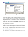
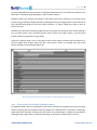
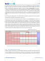
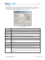
Software Trend Analyzer
User Manual
for SolidSTA v1.3
March 2010
© 2007-2010 SolidSource BV
www.SolidSourceIT.com
Page |3
Contents
1
Introduction .......................................................................................................................................... 5
1.1
Supported configurations ............................................................................................................. 5
2
Installation ............................................................................................................................................ 5
3
Main functions ...................................................................................................................................... 6
3.1
GUI layout ..................................................................................................................................... 6
3.2
SolidSTA project management...................................................................................................... 8
3.2.1
Creating a new project .......................................................................................................... 8
3.2.2
Loading a project................................................................................................................... 9
3.2.3
The code browser window .................................................................................................... 9
3.2.4
Step 1 – Retrieving the files list ........................................................................................... 11
3.2.5
Step 2 – Retrieving change information ............................................................................. 11
3.2.6
Step 3 – Retrieving file content information....................................................................... 12
3.2.7
Information retrieval and the project evolution view ........................................................ 12
3.2.8
Getting information on the retrieval process ..................................................................... 12
3.3
Managing selections ................................................................................................................... 13
3.4
Project evolution view ................................................................................................................ 14
3.4.1
File layout ............................................................................................................................ 14
3.4.2
Defining snapshots and a focus interval ............................................................................. 14
3.4.3
Ordering files on the vertical axis ....................................................................................... 15
3.4.4
Grouping files ...................................................................................................................... 16
3.4.5
Advanced file sorting options ............................................................................................. 16
3.4.6
Other file operations in the evolution view ........................................................................ 17
3.4.7
Zoom and pan ..................................................................................................................... 18
3.4.8
Magnitude bar..................................................................................................................... 18
3.4.9
Making selections ............................................................................................................... 19
3.4.10
Showing detailed version information ................................................................................ 19
3.5
Visualizing metric values ............................................................................................................. 19
© 2007-2010 SolidSource BV
www.SolidSourceIT.com
Page |4
3.5.1
Authors................................................................................................................................ 20
3.5.2
File type ............................................................................................................................... 20
3.5.3
Find text .............................................................................................................................. 20
3.5.4
Folder .................................................................................................................................. 20
3.5.5
McCabe’s complexity .......................................................................................................... 21
3.5.6
Methods .............................................................................................................................. 21
3.5.7
Code size ............................................................................................................................. 21
3.5.8
Debugging activity:.............................................................................................................. 21
3.5.9
Customizing the color encodings for metrics ..................................................................... 22
3.5.10
Showing the evolution of a metric ...................................................................................... 24
3.5.11
Value enhancing options for the metrics ............................................................................ 24
3.5.12
The preset controller .......................................................................................................... 24
3.6
Trend view................................................................................................................................... 25
3.7
Computing software metrics ...................................................................................................... 27
3.8
Computing evolution clusters ..................................................................................................... 28
3.8.1
Selecting the level-of-detail of showing clusters ................................................................ 29
3.8.2
Selecting the right level-of-detail ........................................................................................ 30
3.9
4
Settings........................................................................................................................................ 32
Usage examples .................................................................................................................................. 33
4.1
A First Look on the Project .......................................................................................................... 33
4.2
Finding the Authors..................................................................................................................... 34
4.3
Visualizing evolution trends ........................................................................................................ 35
4.4
Localizing folders of intense activity ........................................................................................... 37
© 2007-2010 SolidSource BV
www.SolidSourceIT.com
Page |5
1 Introduction
SolidSTA (Software Trend Analyzer) is a software application that helps understanding, analyzing and
managing the evolution of software projects recorded in software versioning repositories such as
Subversion or CVS. SolidSTA enables users to discover and analyze various correlations that exist
between the data stored in a software repository, such as the file structure, the project team, the
change moments, and various software quality and complexity indicators. Such analyses are useful in a
variety of scenarios, such as performing quality assessments of previously unknown software as a due
diligence investigator; taking decisions for releasing, refactoring, or migrating software as a project
architect; monitoring development and maintenance progress as a project leader; and learning a new
software stack as a new project member.
1.1 Supported configurations
The SolidSTA analysis tool is an end-user client application which connects itself with the server hosting
the actual software repository to perform the analysis. The current version of SolidSTA supports out-ofthe-box investigations of Subversion and CVS repositories. Other repository types are supported on
demand via customized plug-ins1.
In order to run SolidSTA, the following minimal configuration is required:
Operating system: Windows 2000, NT, XP or Vista (32bit), Windows 7 (32bit) or Linux;
Memory: 512 MB minimum, 2 GB advised;
Graphics card: OpenGL 1.0 compliant in full-color (RGBA) mode, resolution of 1024 x 768
minimum, 1280 x 1024 or higher advised;
Hard disk space: 100 MB free minimum. The actual amount of free space required is dependent
on the size of the analyzed repository and the type of analysis being performed.
2 Installation
This section describes the installation of SolidSTA. We assume further that the reader has the
appropriate installer for the considered platform. For Windows, this is a wizard-based executable
application.
When running the installer (which is for the largest part self-explaining), you will be offered the option
to select from several modes. The minimal mode installs only the strictly required components, and uses
minimal disk space. The full mode installs also some examples of datasets from already analyzed
repositories, and can be used to learn the functions of SolidSTA without having to first connect to a
remote repository. However, this mode requires extra free disk space.
1
Existing SolidSTA clients use the tool with custom developed plug-ins for GIT, PVCS, CM Synergy and Clearcase
repositories.
© 2007-2010 SolidSource BV
www.SolidSourceIT.com
Page |6
3 Main functions
In this section, the main functionality of SolidSTA is described. After reading this, you should be able to
perform a basic scenario: connect to a repository, get the data, compute some quality indicators and
visualize them. To get a better understanding of how SolidSTA can be used to answer real-life, complex
questions, the reader is advised to study the use case examples described in Section 4.
3.1 GUI layout
SolidSTA comes as a Graphics User Interface (GUI) with a multi-window environment. Most windows
have a fixed or anchored position in the tool layout and can only be hidden or shown2. The main
components of the layout are depicted in Figure 1. They are:
1. The metric selection panel. This is used to select the SolidSTA quality indicators (i.e., metrics)
that are displayed as colors in the project evolution view.
2. The preset controller. This is used to control the way in which multiple metrics are combined
into the color used in the project evolution view. The preset controller is further presented in
Section 3.5.12
3. The view selector. This is used to select which windows, or data views, are shown on the screen
at a given moment (see Figure 2).
4. The code browser. This is used to browse the source code of a project and to retrieve evolution
information. The code browser is further described in Section 3.2.
5. The project evolution view. This is used to display the evolution of (a selection of) files from a
software project. This window is one of the most important work areas of SolidSTA. The
evolution view is further described in Section 3.4.
6. The top menu. This is used to manage the extraction and analysis projects, and to control the
various tool settings.
2
The exceptions are the version info display (further described in Section 3.4) and the command log (described in
Section 3.2), which are floating windows.
© 2007-2010 SolidSource BV
www.SolidSourceIT.com
Page |7
6
1
2
3
4
5
Figure 1: Main GUI components
Detailed version information
Code browser
Metric trend view
Command log
Figure 2: View selector (on/off)
© 2007-2010 SolidSource BV
www.SolidSourceIT.com
Page |8
3.2
SolidSTA project management
3.2.1 Creating a new project
To start working with SolidSTA, one needs first to create a new project. This can be done using the
[File→New…] entry in the top menu. A project settings dialog appears (Figure 3). Next, input the
address of the desired repository which you want to analyze. The format of this address depends on the
actual settings used when the repository was created.
For example, assume you have a Subversion repository which you would check out using a command
like:
svn checkout --username guest svn://svn.win.tue.nl/repos/MCRL2 MyWorkingFolder
Figure 3 shows how the required information needs to be filled in for the check-out command shown
above.
Figure 3: The project settings dialog
Project name
This field is used to give a local name to the project. You can input here any name
you like. The project will be listed under this name in the available project table that
is used for loading an existing project (Figure 4).
Project type
Protocol
These fields have to be set depending on the actual repository type. For example, a
Subversion (SVN) repository admits several protocol types, such as svn, http, https,
or file, whereas a CVS repository uses different protocols (e.g., pserver). Depending
on the protocol, several additional fields may be shown.
URL
This field is the address where the repository is located, without the svn:// prefix.
User name
This field is the actual name which will be used to connect to the repository. If a
password is required for that user name, it will be asked later during the project setup.
© 2007-2010 SolidSource BV
www.SolidSourceIT.com
Page |9
Finally, note that SolidSTA does not need the name of the local working folder where to transfer the
repository data, e.g. MyWorkingFolderin the above command line. SolidSTA will cache only the required
repository data, which is a small part of the total repository size, in its internal database.
Figure 4: The open analysis project dialog
After filling in the project settings, the new created project will appear in the list of available projects,
which can be displayed using the [File→Open…] entry in the top menu. By pressing the [Load] button
(see Figure 4), the newly created project is made active. All commands from this point will be run on this
project. At this point, a password is also asked for future access to the associated repository. If the
actual user and repository combination does not require a password, or if you want only to access the
data cached locally by SolidSTA, you can simply press the Esc key. By pressing the Enter key in the
password field you indicate that a password is needed and that this is empty3.
3.2.2 Loading a project
Selecting an existing entry in the list of available projects does not automatically make the project
active. For this, you should use the [Load] button or to double-click the project name. After loading a
project, the code browser window displays the information that has been previously retrieved from the
project’s repository in an earlier work session with SolidSTA, if any (see Figure 5). In case of a new
SolidSTA project, no information has been retrieved yet from the associated repository, so the code
browser will be empty.
3.2.3 The code browser window
This window shows a file tree view of the already loaded information from the repository, and the saved
selections during previous analysis sessions. The file (or folder) names shown here indicate the files or
folders in the repository at the last time when SolidSTA did connect to the repository. The names of
these files and folders (not their files’ contents, though) are locally cached by SolidSTA. To be sure that
this information is always up-to-date, you need to synchronize it with the associated repository by
3
Some repositories (e.g., Subversion) can make a distinction between a (required) empty password and a not
required/unknown password.
© 2007-2010 SolidSource BV
www.SolidSourceIT.com
P a g e | 10
pressing the [Update file list] button in the information acquisition control panel at the bottom of the
window (Figure 5).
Saved selections
File tree
Progress
indicators
Control panel for
acquiring evolution info
Update
file list
Clear
file list
Update
history
info
Clear
history
info
file list
Update
snapshot
contents
Cancel
operation
Figure 5: The code browser displays previously retrieved files and controls the acquisition of evolution information
The colored icon shown in front of a file name indicates the type of information cached locally by
SolidSTA for that file (see also Figure 5):
© 2007-2010 SolidSource BV
www.SolidSourceIT.com
P a g e | 11
a white icon indicates that no information about that file is present in SolidSTA, except the file
name.
a pink icon indicates that SolidSTA has already cached change information about the commit
moments of that file, the authors4 of the changes (commits), and the commit logs. If this
information is available, basic evolution investigations can be performed on the associated file.
Bringing information from a repository is an incremental process. Not all information is retrieved in one
single step. Instead, the process is divided in three steps:
3.2.4 Step 1 – Retrieving the files list
First, a file list of the files available in the repository needs to be retrieved. For this, press the [Update
file list] button (Figure 5). Depending on the type of repository and the network connection, this can be
a time consuming operation5. During this process, an update being processed indicator is displayed in
the progress indicator area of the code browser window (Figure 5). This indicator is actually displayed
every time an operation modifying the cached information is performed by SolidSTA, e.g. update the
files list, clear the files list, etc.
Figure 6: Indicator for an update being processed in the “Progress indicators” area of the code browser
You should use the [Update file list] button every time you desire to be sure that the locally cached files
list is synchronized with the actual files list in the repository. This action is quite similar to the periodic
check-out command issued by developers via their local Subversion clients.
3.2.5 Step 2 – Retrieving change information
After retrieving the files list, the next step is to retrieve the change history information of one or several
files from the associated repository. For this, first select the files of interest in the code browser. By
default, all files, i.e. the entire tree shown in the code browser, are selected. However, if the project is
very large, retrieving change information for all those files can be a time consuming operation. Also, in
some cases, one is only interested in quickly examining the evolution of a subset of files, for example a
particular folder.
In such cases, you want to select a subset of the entire file tree shown in the browser. To select a folder
in the tree, click using the left mouse button on the respective folder item in the tree browser. This will
create a new selection having the folder items as contents. You can then process only this selection
further, for example to retrieve change information. Additional information on managing selections is
discussed in Section 3.3.
Once a selection is available, press the [Update history info] button in the code browser window (Figure
5). This will initiate a connection to the repository and locally bring the change information, or version
list, for the selected files. The change information is the minimum required in order to perform basic
investigations on the evolution of a project.
4
5
In this document, we use the terms authors and developers interchangeably.
Subversion repositories, as opposed to CVS ones, should be quite fast at this step.
© 2007-2010 SolidSource BV
www.SolidSourceIT.com
P a g e | 12
3.2.6 Step 3 – Retrieving file content information
The third and last step is to retrieve information on the actual content of one or several files for a
defined set of snapshots (i.e., time moments). For detailed information on defining snapshots see
Section 3.4.2. Just as for the retrieval of change information, this can be a lengthy process, as the actual
file contents of all defined snapshots of the selected set of files must be transferred from the repository.
Hence, making a selection of the files of interest is also recommended in this case. After making this
selection, press the [Update snapshot contents] button in the control panel window. This will initiate a
connection to the remote repository and transfer the contents of the defined snapshots of the selected
files. The file content information enables SolidSTA to compute code metrics and performed in-depth
investigations on the evolution of a project.
If updating the contents of a given selection takes too long, e.g. because of a too slow connection or
because the selection to update is too large, you can press the [Cancel operation] button in the code
browser window.
3.2.7 Information retrieval and the project evolution view
During the three steps of information retrieval, the project evolution view will change its appearance, to
indicate the actual amount of information currently available locally to SolidSTA. Figure 7 shows the
project evolution view in its three states: before retrieving the file list (a); after retrieving the file list but
before retrieving the change history (b); and after retrieving the change history (c). The actual meaning
of the information presented in the evolution is described in the next section.
a)
b)
c)
Figure 7: Project evolution view during the three steps of retrieving information from a repository:
a) before retrieving the file list; b) after retrieving the file list but before retrieving the change history; c) after retrieving the
change history.
3.2.8 Getting information on the retrieval process
When performing the above retrieval operations (file list, change history, and contents), the Update
being processed indicator is displayed (Figure 6). One can get more detailed information about the
status of the update operation by displaying the command log window. For this, press the [Command
log] button in the view selector (Figure 2).
© 2007-2010 SolidSource BV
www.SolidSourceIT.com
P a g e | 13
3.3 Managing selections
A typical repository contains thousands or even tens of thousands of files. Clearly, it is not practical to
analyze or visualize all these files in the same time. To help coping with scale, SolidSTA lets users
perform all its operations on subsets of the entire repository. Such a subset of files and folders is called a
selection. In this section we explain how selections can be managed. The actual operations on selections
are described in the other chapters of this manual.
evolution view
selection view
Pop-up menu → Save
selection
click
SHIFT+ click
CTRL+click
CTRL+click
file browser
click
selection saving
selection loading
Figure 8: Managing file selections in SolidSTA
Blue arrows indicate selection creation, red arrows indicate selection usage
Figure 8 shows the management of selections in SolidSTA and the widgets involved in this process. The
available selections are displayed in a selection view. Clicking on a selection in this view makes it the
target of subsequent analysis operations. For example, this selection becomes the input of the
visualization shown in the project evolution view (see Section 3.4 on the project evolution view).
Selections can be created in different ways. The easiest way is to click on a folder in the file browser
view. The respective folder (and all its contents) will be added to a new selection that will be loaded in
the evolution view. By holding down the CTRL button during this process, the selection will be saved in
the selection view for further reference, and its name will be the same as the folder name.
A second, more involved method to create selections uses the evolution view, as explained further on in
“Making selections” (Section 3.4.9)
© 2007-2010 SolidSource BV
www.SolidSourceIT.com
P a g e | 14
3.4
Project evolution view
The project evolution view is one of the main work areas of SolidSTA. This view displays the evolution of
a selected set of files from all files existent in the repository. As explained, the minimum amount of
information required by this view is the change information for the files in the selected set. This can be
retrieved using the [Update history info] button in the button in the code browser window (see Step 2 –
Retrieving change information in Section 3.2.5).
The project evolution view offers several investigation tools for the evolution of the files. These are
described next.
3.4.1 File layout
Once the change information is cached, the history of each file is depicted as a horizontal stripe, made
of rectangular segments (Figure 12). The evolution of the entire set of selected files in the evolution
view is depicted as a stack of horizontal stripes, one per file, one atop the other. The horizontal axis
encodes time. The vertical axis stacks the files in the selected file set.
In the default mode, each file appears as a dark grey stripe, starting at the moment when the file was
first committed to the repository. Thin brown vertical lines indicate when the file has been changed
after the creation moment, so they correspond to the commit moment of a new file version (Figure 9). A
timeline bar is displayed atop of the project evolution view.
commit moments
file start moment
timeline
Figure 9: Timeline, files, and commit moments in the evolution view
3.4.2 Defining snapshots and a focus interval
Snapshots are time instances defined by the SolidSTA user within a given project evolution time frame.
These time instances are used as reference moments when acquiring content information (see Section
3.2.6). A focus interval is a time interval defined by the SolidSTA user within a given project evolution
time frame. This interval is used to focus analysis activities on a specific evolution interval (e.g., sorting
files on activity → see Section 3.4.3). Both snapshots and the focus interval are mechanisms for focusing
the analysis on specific moments or periods during the evolution of a project, and can greatly speed-up
analysis tasks for large projects.
© 2007-2010 SolidSource BV
www.SolidSourceIT.com
P a g e | 15
Focus interval
Snapshot marker
Clear focus
interval
Snapshot pop-up menu
Figure 10: Snapshots and focus interval
To create a snapshot, double-click the left mouse button in the timeline area of the project evolution
view. To edit the snapshot properties double-click the left mouse button on the snapshot marker. A
pop-up menu will appear with three alternatives: change the name of the snapshot, delete the snapshot
and select a calendar date.
To create a focus interval, click and drag the right mouse button in the timeline area of the project
evolution view. To clear the interval, press the [Clear focus interval] button in the top right corner of
the view (Figure 10).
3.4.3 Ordering files on the vertical axis
The ordering of events on the horizontal direction is fixed, given by time. However, the ordering in the
vertical direction can be changed, according to various criteria. The various file sorting options are
available by clicking the right-mouse button in the evolution view. This shows a pop-up menu with
several sorting options. Files can be sorted on:
Type: files are sorted based on their type, i.e. extension. Files with the same extension come
one after the other.
Creation time: files are sorted based on the moment when they have been first committed to
the repository.
Activity: files are sorted based on the number of versions they have in the current focus interval
(see Section 3.4.2). Files with many versions, i.e. changed many times, are placed at the top of
the evolution view. Less active files are placed at the bottom.
Text searches: when using the “Find text” plugin (see Section 3.5.3), files are sorted based on
the number of versions in which a given text search occurs.
Local similarity: when a file is selected in the project evolution view (see the ‘Making Selections’
section below), files will be sorted based on their evolution similarity with the selected file.
Similar transaction: files are sorted such that the files that have been committed in the same
transaction as a so-called ‘reference transaction’ appear at the top. The reference transaction is
© 2007-2010 SolidSource BV
www.SolidSourceIT.com
P a g e | 16
indicated by the position of the mouse pointer along the horizontal (time) axis in the evolution
view at the moment when the sorting pop-up menu was invoked.
Invert sort: the order of files in the vertical direction is reversed.
Sort operations
Group operations
operations
Figure 11: The pop-up menu in the evolution view enables changing the order of files in the vertical direction
3.4.4 Grouping files
Besides sorting, we also would like to group files based on the computed metrics. The [Group selected]
option in the right-button menu of the evolution view allows doing that. This submenu lists all visible
metrics (see Section 3.5 on how to make metrics visible). Grouping on a metric listed in this menu will
arrange files, in the evolution view, so that those files having the same value of that metric come one
after the other.
Note that the meaning of ‘having the same value of a metric’ strongly depends on the metric type and
the metric values selected in the respective color encoding
3.4.5 Advanced file sorting options
Besides sorting the files in the evolution view based, files can also be grouped in more complex ways,
based on their evolution similarity within the current focus interval (see also Section 4.4). This more
advanced feature is available via the [Compute clusters] entry in the pop-up menu.
© 2007-2010 SolidSource BV
www.SolidSourceIT.com
P a g e | 17
When displaying software metrics (see Section 3.5), a selection of files based on metric values can be
made. The [Group selected] entry in the pop-up menu enables the user to choose the metric based on
which the file selection will be performed.
‘Fit all’ zoom button
Timeline
scale
‘Fit to bar’ zoom button
Magnitude bar
Figure 12: The decorations of the project evolution view
The evolution view contains a number of controls which show information and also allow performing
several navigation functions (see Figure 12). These are explained below.
3.4.6 Other file operations in the evolution view
Besides sorting and grouping, the pop-up menu of the evolution view (see Figure 11) offers a number of
additional operations that can be useful during analysis.
Compute similarity: computes an evolution similarity measure to be displayed in the vertical
magnitude bar. The reference file for this similarity measure is the file currently pointed at with
the mouse.
Remove transaction: removes from the evolution analysis the commits that are similar to the
one pointed with the mouse. This operation is useful for discarding cross-system transactions
related to, for example, code beautification.
© 2007-2010 SolidSource BV
www.SolidSourceIT.com
P a g e | 18
Remove cross-system transactions: creates a list of cross-system transactions that are
candidates for discarding from the analysis. This option is useful for filtering out transactions
that refer to uninteresting development events such as code beautifications, when a large part
of the system is updated, without a change in the functionality of the system.
Remove selected versions: removes from the evolution view all commits that are marked using
a metric value widget (see Section 3.5).
Save selection: saves the current selection of files and commits (see Section 3.3).
Save frequency list: saves the list of files in the current selection together with an indication on
the amount of commits in the current focus interval. The data is saved using a comma separated
values format, and can be imported for further processing in other applications.
Take snapshot: saves a snapshot image of the evolution view in the PNG graphics format. This
option is useful for saving analysis images, for example, for later use in a report, or for posting
on the web.
3.4.7 Zoom and pan
When the number of files displayed in the project evolution view is too large, one can get detailed
information by zooming in and by panning the view. This can be done using the preset zoom buttons of
the project evolution view (see Figure 12). The [Fit to bar] button zooms in so that the file stripes are
large enough for one to see their detailes, e.g. names. The [Fit all] button zooms the view out, thereby
reducing all file stripes to thin pixel lines. This mode is useful when one is interested in obtaining an
overview of a large project.
Besides these preset zoom levels, one can manually control the zoom factor by:
pressing CTRL and rolling the mouse wheel (for the vertical direction)
pressing CTRL+ALT and rolling the mouse wheel (for the horizontal direction)
The scroll bars can be used for panning (scrolling) the view.
3.4.8 Magnitude bar
At the left side of the project evolution view we see a thin vertical bar. This bar can be used to display
various metrics computed on the entire history of a file.
So far, the metrics that can be displayed in the magnitude bar are:
the activity of a file, or its number of versions ;
the text hits, or number of commit logs of a file in which a given text occurs;
evolution similarity of all files to a reference file.
These metrics are also used as criteria for sorting the files (see earlier in this section).
© 2007-2010 SolidSource BV
www.SolidSourceIT.com
P a g e | 19
The displayed metric in the magnitude bar can be chosen by pressing the red arrow button at the
bottom of the bar. The name of the actual selected metric is shown in the Settings tab of the Control
Panel. In the same tab, one can also specify how the metric will be displayed. Available alternatives are
bar charts and a blue-to-red color rainbow map (see also Section 3.9).
3.4.9 Making selections
The project evolution view allows the user to make various selections of files. Selections enable users to
focus their investigations on a group of files, as explained in Section 3.3. Selections are also useful for
speeding up the data retrieval operations (discussed in Section 3.2), as these operations are only
executed on the set of selected files.
Selections can be done in the evolution view, similar to list selections in other programs. A mouse click
selects one file. Pressing SHIFT while clicking the left mouse button selects groups of contiguous files.
Pressing CTRL while clicking the left mouse button enables selecting individual files. Releasing the SHIFT
or CTRL key creates the selection, which gets added to the selection view, and also becomes the target
shown in the evolution view.
By default, selections are made by keeping the selected files from a larger set. If desired, selections can
be made by eliminating the selected files away and keeping the rest (i.e., a negative or subtractive
selection). This can be done by holding down the ALT keys while making the selection using the above
procedure.
3.4.10 Showing detailed version information
This window is used to display detailed information about a single file version. When this window is
enabled, using the views selector (see Section 3.1), it shows the log message left by the committer, or
author, of the file version at which the mouse points in the project evolution view. Moving the mouse in
the evolution view dynamically updates the contents of the version information window.
3.5 Visualizing metric values
SolidSTA enables the user to visualize a wide range of metrics6 and quality indicators concerning the
evolution of files in a given repository. For each version of each file in the evolution view, the value of
the selected metric of interest is typically encoded as the color of the stripe segment corresponding to
the respective version.
When several metrics are available for a project, users can choose which to display using the leftmost
widget (checkbox list) in the Metrics tab of the Control Panel. Figure 13 shows the Authors and
McCabe’s complexity metrics made visible from the list of available metrics. For information on how to
compute various evolution metrics in SolidSTA, see further Section 3.7.
For each visible metric, the Metrics panel shows a separate widget displaying how the values of that
metric are mapped to colors. These widgets are called metric value widgets. For example, Figure 13
6
By metric, or indicator, we understand here any data attribute which is associated with a file version, whether
numerical (e.g. age or size), textual (e.g. file name) or categorical (e.g. author ID or extension)
© 2007-2010 SolidSource BV
www.SolidSourceIT.com
P a g e | 20
shows the Authors and McCabe’s complexity metric-value widgets to the right of the list of available
metrics.
Metric value widgets are used to customize the way we map metric values to colors. Since these
mappings are quite specific for various metric types, they are implemented as customizable plug-ins in
SolidSTA. Hence, different types of metrics can have different types of metric value widgets.
The entries in the color encoding widgets are clickable and editable, so users can for example change
the colors used for particular metric values. Also, when one or more values are selected in a color
encoding widget, only the file versions having those values will be shown in the evolution view. This can
be used to perform simple but useful analyses like “show all file versions committed by author X”. For
this, you would need to enable the Authors metric, and then select in its color encoding widget the entry
for the author called X. Several entries in a list can be selected in the same time. To deselect all entries
in a list, make the metric for that list invisible (uncheck it in the leftmost list widget in the Metrics tab),
and then check it back on.
A number of metrics, with corresponding color encodings, are available in SolidSTA by default. These are
the Authors, File type, Find text and Folder metrics. Other metrics are available as optional plug-ins.
Optional metrics include the McCabe complexity, Methods, Code size and Debugging activity metrics.
Other optional (custom-built) metrics may be available (provided by SolidSource or other parties that
are licensed to build SolidSTA plug-ins).
3.5.1 Authors
The ID of the author who committed a given file version is mapped to colors. A slider at the bottom of
the list of authors enables users to indicate a decay factor for the ‘knowledge’ an author has about the
system. This is useful when visualizing trends of knowledge distribution (see Section 3.6).
3.5.2 File type
The file type, i.e. extension, is mapped to colors.
3.5.3 Find text
The versions whose commit logs contain a given text are mapped to colors. The Find text color encoding
widget contains an interface to add and remove text fragments to search for, and also to customize the
colors of the file versions whose logs contain those texts. Versions whose commit logs contain two or
more of the searched keywords are displayed in a predefined color – red.
3.5.4 Folder
The path to which a file belongs is mapped to colors. In other words, files on the same path will be
shown using the same color. A slider at the bottom of the folder list enables users to control when two
files are considered to be on the “same path”. Consider a file f1 with the path /usr/files/foo/f1 and a file
f2 with the path /usr/files/bar/f2. The slider at the bottom of the Folders color encoder widget controls
the number of path elements, counted from the root downwards, used when checking if two files are on
the same path. For example, if this slider has the value 1, only the first path element is compared. In our
example, since both f1 and f2 are in /usr, they will be considered on the same path. If the slider has the
© 2007-2010 SolidSource BV
www.SolidSourceIT.com
P a g e | 21
value 2, the first two path elements are compared, i.e. /usr/files in our example. Again, f1 and f2 will
then be considered as being on the same path. If the slider has the value 3, then f1 and f2 will not be
considered to be on the same path, since the third element of f1’s path is ‘foo’ whereas this is ‘bar’ for
f2. The Folder metric is useful in visually highlighting files which are close in the directory structure of a
project.
3.5.5 McCabe’s complexity
This metric encodes the so-called McCabe, or cyclomatic, complexity of a source code file. This is a wellknown measure in software engineering of the complexity of a fragment of code. Intuitively, the
cyclomatic complexity of a piece of code is equal to the number of alternative execution paths, or
decision points, in the code. Code with high cyclomatic values, e.g. functions with a complexity larger
than 10..20, is considered complex to understand and maintain. Alternative aggregations of this metric
are given in a drop-down list. This allows displaying the McCabe’s complexity for different units of code.
The slider at the bottom of the list allows controlling the range units used for coloring. Higher slider
values aggregate larger ranges into the same color, and are useful when the total range of the
complexity is high. Smaller slider values use finer ranges (smaller intervals) per color, and are useful
when the total range of the complexity is lower.
The McCabe’s complexity color encoder is only available in a project where the McCabe metric has been
previously computed using a metric calculator (see Section 3.7). Also, note that this value is computed,
thus visualized, only for certain source code files (e.g. C, C++, Java), and definitely not for non-sourcecode files, (e.g. images).
3.5.6 Methods
The methods metric gives a list of all methods and plain functions in a project and encodes the presence
of a method in a given version. This color encoder is only available in the project where the project
methods have been previously identified using a metric calculator (see Section 3.7). As for the McCabe’s
complexity, this metric is only computable on certain types of source files (C, C++, Java).
3.5.7 Code size
The Code size metric encodes the size of a project, counted in lines of code (LOC) using various
alternative aggregations which are available in a drop-down list. The displayed value intervals can be
adjusted using the slider at the bottom of the list. This color encoder is only available in the project
where the size metric has been previously computed using a metric calculator (see Section 3.7). As for
the Methods or McCabe’s metric, this metric is only computed for source code files (C, C++, Java).
3.5.8 Debugging activity:
The Debugging activity metric encodes the location of the reports on debugging activity based on
information provided by Bugzilla databases. This color encoder is only available in the project where bug
fixing activities have been previously computed using a metric calculator (see Section 3.7).
© 2007-2010 SolidSource BV
www.SolidSourceIT.com
P a g e | 22
Figure 13: The Metrics tab of the control panel. The leftmost list shows the Authors and McCabe’s complexity metrics made
visible (checked). The middle and right lists show the color encodings for these two metrics.
3.5.9 Customizing the color encodings for metrics
The colors assigned by encoders to a given value or interval can be changed using the [Change color]
entry in the pop-up menu associated with each color encoder list (see Figure 15).
The color encoder widgets can also be used to display statistics associated with each entry in the list. By
choosing the [Show statistic_name] type of entries in the associated right-mouse pop-up menu, a blue
bar that indicates the value of that statistic is displayed for each entry in the list. Also, the list can be
sorted increasingly or decreasingly on the value of this statistic.
For example, Figure 14 shows the color encoder widget for the Authors metric, after the [Show
#versions] statistic is enabled, and with the author IDs sorted in increasing order of the ‘#versions’
statistics. This sorting, as well as the colored bars in the list widget, clearly show that keithp, the author
at the bottom of the list, is responsible for about 60% of the total number of versions in the project
evolution. His color is red. Looking at the file versions in the evolution view, we can see when, and which
files, did he modify.
© 2007-2010 SolidSource BV
www.SolidSourceIT.com
P a g e | 23
Figure 14: File versions colored by author metric. The Authors color encoding widget shows the authors sorted in increasing
order of number of committed versions
Value enhancer entries
Export entries
Sort entries
Show metric entries
entries
Figure 15: Pop-up menu associated with a color encoder list
© 2007-2010 SolidSource BV
www.SolidSourceIT.com
P a g e | 24
3.5.10 Showing the evolution of a metric
The color encoding widgets let users control how a metric is displayed in the evolution view. However,
in some cases, we are interested to see a simpler, more aggregated, view of the evolution of a given
metric. The [Show evolution] entry in the color encoder widget’s pop-up menu can be used to display
trends in the metrics associated with a color encoder. The trend display widget is discussed separately in
Section 3.6.
3.5.11 Value enhancing options for the metrics
The pop-up menu in the color encoder widgets contains also a number of value enhancing options.
These are more advanced, but potentially less intuitive, mechanisms for displaying data in the evolution
view using texture markers. The available options are as follows:
Marker center: makes visible the presence of a version associated with the selected color
encoder list entry. This can be used when the versions are so close to each other that the
segments are not visible anymore, so color identification alone is not enough.
Marker density: Gives an indication of the number of versions associated with the selected color
encoder list entry. This can be used when the versions are so close to each other that the
segments are not visible anymore, so color identification alone is not enough. This enhancer is
most commonly used in combination with the previous marker (i.e., Marker center). The
previous marker shows existence of at least a version, this one indicates the number on
versions.
3.5.12 The preset controller
The Metrics tab of the Control Panel offers a list of available color/texture encoders that can be used to
display metric values on the file version segments of the project evolution view. Easily switching
between these encoders can facilitate discovery of correlations between the various metrics. The preset
controller can be used to do this switching (see Figure 16).
a
c
b
Figure 16: The preset controller enables easy switching between color encodings
© 2007-2010 SolidSource BV
www.SolidSourceIT.com
P a g e | 25
The preset controller works as follows. At any moment, the user can enable more color encodings by
using the color encoder check list in the Metrics tab of the Control Panel. For each enabled encoder, an
icon is displayed in the preset controller. Figure 16 displays a preset controller with three enabled color
encoders: Authors, McCabe complexity and Find text.
The preset controller contains also a special icon surrounded by color disks of decreasing luminance: the
Observer. The relative position of the observer with respect to the other icons determines the color that
will be actually painted on the version segments in the project evolution view. To understand how this
works, drag he observer with the mouse towards any of the icons. You will see how the color of the
version segments in the evolution view changes to the color of the icon’s encoder. In other words, when
the Observer is close to (or on), say, the Authors icon, the color shown in the evolution view encodes the
Authors metric. When the Observer is somewhere between the icons, the actual color used in the
evolution view is a blend of all colors given by the enabled encoders, weighed by the distances of their
respective icons to the Observer. Here, icons which are closer to the observer contribute more to the
final color in the evolution view than icons which are far away from the Observer.
The power of the preset controller becomes visible when we have several metrics that all map to color
in the evolution view and we want to quickly switch between them. For this, we can quickly drag the
Observer in the preset controller towards the desired metric icons and notice the color changes in the
evolution view.
3.6
Trend view
The trend view is the second most important view of SolidSTA, after the evolution view. The trend view
enables users to look at aggregated, simple-to-follow, trends in metrics. To display trends, one needs to:
Enable the trend view by using the data views selector (Figure 2)
Choose a trend to display by selecting the ‘Show evolution’ entry in the pop-up menu of the
associated color encoder value list (Section 3.5.10, “Showing the evolution of a metric”)
The trend view shows graphics of aggregated values, such as, for example, the trend of the total
complexity in the system. Alternatively, the trend view can also show the evolution of the number of
files or file versions matching a given criterion. The selection of the type of trend to display is done using
the associated pop-up menu of the trend view (see Figure 17).
© 2007-2010 SolidSource BV
www.SolidSourceIT.com
P a g e | 26
Graphics type
View type
Figure 17: Pop-up menu for the trend view window
When the values presented in the color encoder list are categorical, e.g. they indicate the ID of a person,
one can count the number of files or file versions that match a number of selected entries in the list for
a given time interval. The time interval can be adjusted by pressing CTRL and using the mouse wheel in
the trend view.
The different graphs displayed in the trend view can be drawn using various graphic metaphors: bar
charts, line graphs, intensity (luminance) or color rainbow maps, and flow graphs. These types of
graphics are selectable using the pop-up menu in the trend view.
Figure 18 illustrates the trend view. This image shows the evolution of the number of files that have
been committed by three authors, indicated by the three different colors, using a sampling interval of 1
month and a Flow graph type. This view has been obtained by selecting the three authors in the Authors
color encoder list and choosing the Show evolution entry in its associated pop-up menu. This view is
useful in showing how the amount of files modified by each author, which can be seen as an
approximation of the ‘knowledge’ that author has on the entire project, varies in time.
Figure 18: Trend view for the knowledge distribution using the Authors color encoder
© 2007-2010 SolidSource BV
www.SolidSourceIT.com
P a g e | 27
Figure 19 shows the evolution of the software complexity in a system using the McCabe complexity
metric. The sampling interval is 1 month yet the data is available only for two snapshots. The snapshots
are the only moments when the complexity of the system can be probed (see Section 3.7). The used
graphics type is bar chart, and the type of view is Average value. This trend view was enabled by
selecting the Show evolution entry in the pop-up menu associated with the Complexity metric color
encoder. This view shows how the complexity of the code in the given project increases significantly
during the project’s lifetime. This is a typical indication of a project that becomes hard(er) to maintain.
Snapshot 1
Snapshot 2
Figure 19: Trend view of software complexity using the McCabe complexity color encoder
3.7
Computing software metrics
The color encoders available in SolidSTA need pre-computed metric information in order to operate.
Some basic metrics are available by default when retrieving the change information stored in software
repositories, e.g. author ID, file type, and commit log messages. Additional software metrics can be
computed on demand (depending on the available plug-ins), for example based on the source code,
such as the McCabe complexity metric. For the latter type of information, the third step of retrieving the
file content data presented in Section 3.2 is required. One should mind the fact that metrics based on
source code can be computed and made available for the snapshot moments only.
In the following, we briefly describe the procedure of computing software metrics which need access to
the files’ contents. Once all information regarding the file contents has been retrieved and cached
locally by SolidSTA, software metrics can be computed using a number of algorithms available as plugins. This can be done from the Compute metrics dialog (see Figure 20). This dialog can be displayed by
choosing the [Tools → Compute metrics…] entry in the top menu.
© 2007-2010 SolidSource BV
www.SolidSourceIT.com
P a g e | 28
Cached metrics
Available calculators
Selected calculator description
Figure 20: The Compute metrics dialog
The list of available calculators is given together with a short description about what the calculators
does, what is the prerequisite information and what type of metrics it can compute. A list of already
calculated metrics, cached by SolidSTA locally, is also given. If desired, an already calculated metric can
be removed from the local cache, e.g. to save memory, clean up the cache, or because we want to
recompute the metric for whatever reason.
To run a calculator, select it from the list and press the [Generate] button (see Figure 20). The
corresponding metrics for that calculator are computed on the set of selected files. Recall that files can
be selected by using either the selection mechanisms of the code browser view (see Section 3.2) or
those of the project evolution view (see Section 3.4).
Usability note: there is no automatic way of determining which metrics are needed by which color
encoders. This is necessary as the input of the latter comes from the output of the former. One needs to
rely on other documentation for understanding the dependency relations between the two. For
example, the Complexity and Code size color encoders require the type of metrics generated by the
Basic metrics calculator. The Debugging activity color encoder requires the type of information
produced by the Bug removal activity monitor calculator.
3.8
Computing evolution clusters
When analyzing a large code base with many versions, it is often interesting to see which files have
similar change moments. Files which change at the same, or similar, moments typically indicate related
software components (or other type of related content). Finding related files is extremely useful in
© 2007-2010 SolidSource BV
www.SolidSourceIT.com
P a g e | 29
recovering dependencies which are been lost during the development or are otherwise unknown to the
developers, estimating change propagation, and for impact analyses.
SolidSTA enables such analyses by looking for files which have similar evolutions in the current focus
interval, using a technique called evolutionary coupling. By looking at change patterns in the evolution of
files, SolidSTA builds groups of files with similar evolution, i.e. which change very often at same or
similar moments.
SolidSTA uses a hierarchical clustering algorithm that first groups files having the most similar evolutions
into so-called clusters, then recursively groups similar clusters into larger clusters, until the entire
project evolution is gathered in a single cluster.
Using the ‘Compute clusters’ entry in the pop-up menu of the project evolution view (see Section 3.4),
one can display these clusters atop of the files. Each cluster is shown as a shaded area, dark at the
borders and light in the middle (see Figure 21).
Figure 21: Files in the evolution can be grouped into clusters based on similar evolution
3.8.1 Selecting the level-of-detail of showing clusters
As explained above, clusters containing files with similar evolutions are grouped recursively into larger
clusters. Choosing the level-of-detail at which to display the created clusters is important in obtaining a
useful view of the evolution. Showing too small clusters is not interesting as it displays too much detail.
Showing too few, large, clusters is also not interesting, as the amount of information is too low.
© 2007-2010 SolidSource BV
www.SolidSourceIT.com
P a g e | 30
To select the desired level-of-detail of the clusters, one can use the [Clusters] tab of the metric selection
panel (see Section 3.1). The Clusters tab shows the different levels-of-detail available. Each level-ofdetail, corresponding to a different set of clusters – hence to a different decomposition of the system –
is shown as a vertical bar. All clusters in a given decomposition are shown as small blocks stacked atop
of each other. The size of a cluster, given by how many files it contains, is indicated by its block’s height.
Decomposition bars to the left of this view contain more blocks, i.e. correspond to fine-grained levels-ofdetail, while bars to the right of the view contain less blocks, i.e. correspond to coarse-grained levels-ofdetail.
The current level-of-detail shown in the evolution view is indicated by a red frame. Users can choose a
decomposition for display by selecting it with a mouse click.
The color of the blocks in the decomposition bars indicate the so-called cohesion of the clusters. A
highly cohesive cluster contains files having highly similar evolutions, i.e. which have been changed at
(nearly) the same moments. Highly cohesive clusters are indicated by dark red blocks. Less cohesive
clusters contain files which change at less similar moments in time, and are indicated by light-blue
blocks. Finally, the least cohesive clusters, which are typically also the largest ones, contain many files
which change at unrelated moments in time, and are indicated by blue blocks. Given that bars at the left
contain small, cohesive clusters and bars at the right contain large, less cohesive clusters, the color in
the decomposition view typically change from red on the left to blue on the right.
Current level of detail
Figure 22: The Clusters tab of the metric selection panel enables the selection of an appropriate clustering level
3.8.2 Selecting the right level-of-detail
Selecting a ‘good’ level-of-detail in the decomposition view can reveal highly useful information and
uncover valuable trends in the evolution of a code base. This information is often simply unavailable
from other source and by other means. However, although the decomposition view assists the user in
© 2007-2010 SolidSource BV
www.SolidSourceIT.com
P a g e | 31
choosing a useful level-of-detail, finding the ‘right’ level-of-detail which shows this information cannot
be completely automated.
As a general guideline, when selecting a decomposition level, one should strive for selecting levels
containing large clusters (shown as large blocks in the decomposition view) but with high cohesion
(shown as dark(er) red colors in the same view). These levels are typically located around the middle of
the decomposition view, like the one shown selected in Figure 22.
© 2007-2010 SolidSource BV
www.SolidSourceIT.com
P a g e | 32
3.9
Settings
This section presents a number of settings that can be used to customize the behavior and appearance
of the SolidSTA application. These settings can be adjusted from the Settings dialog (Figure 23) which
can be displayed using the [Settings → Settings…] entry in the top menu.
Figure 23: The Settings dialog
File size
The size of the file bar (see Section 3.4.6).
Vertical metric
The type of visual metaphor used to display the magnitude bar (see Section 3.4.8).
Cluster edge
The size of the cluster edges when evolution clusters are displayed (see Section 3.8).
Marker density
/size /intensity
Sets the appearance, the size and the intensity of the Marker density (see Section
3.5.11).
File labels
Show/hide file labels in the project evolution view (see Section 3.4.1).
Metric label
Show/hide the name of the metric displayed in the Trend view (see Section 3.6).
Record labels
Show/hide the name of the categorical records displayed in the Trend view (see
Section 3.6).
Time grid
Show/hide the time grid displayed in the Trend view (see Section 3.6).
Time labels
Show/hide the time line labels displayed in the Trend view (see Section 3.6).
Vertical scale
Show/hide the vertical scale label in the Trend view (see Section 3.6).
SCM Retries
The number of attempts for retrieving information from a repository upon initial
failure. This option may be useful when connecting to busy repositories that can kill
connections in order to regulate traffic (e.g., when getting error “21002 connection
closed” in SVN).
© 2007-2010 SolidSource BV
www.SolidSourceIT.com
P a g e | 33
4 Usage examples
In this section, several typical usage examples of SolidSTA are presented. For each example, a use-case is
discussed, and we show how to use SolidSTA, and interpret the produced images, to perform some
given assessments on a given project.
This section assumes you have a basic familiarity with the main concepts, way of working, and user
interface of SolidSTA. These notions are detailed in the first chapters of this user manual.
The use-cases presented here are run on real-life repositories and address real-life problems. However,
the presented analyses are simplified, as compared to a real assessment in the field, in order to focus on
a single, or a few, features of SolidSTA at a time.
4.1 A First Look on the Project
In this study, we consider the mCRL project7. First, load the project from the Projects tab of the control
panel. After a few seconds, you should see the control panel information area showing the name of the
project, the number of files in the repository (approx. 2600 files), and the last update (approx. March
2007). Next, right-click in the evolution view (bottom-right large window) and sort the files on creation
time. You should get a picture similar to the one in Figure 24.
step 2
step 1
Figure 24: A first look on the mCRL project
7
The mCRL analysis database is included in the demo distribution of SolidTA
© 2007-2010 SolidSource BV
www.SolidSourceIT.com
P a g e | 34
The evolution view shows two salient ‘steps’, where the software grows significantly in a very short
period of time (highly presumably, in the same commit transaction). These indicate, with a high
probability, moments when software from outside the repository was added. We also recognize a first
‘silent’ phase of the activity, until step 1, and a final ‘stagnation’ phase, after step 2.
4.2 Finding the Authors
Now let us find out how the team working on the project looked like. For this, go to the Metrics tab in
the control panel, check the Authors metric, and drag the observer (red icon) in the preset controller
towards the newly appeared Authors icon. Next, right click on the Authors list-widget in the Metrics tab,
select [Show #versions], and then [Sort on #versions]. You should now get a view similar to the one in
Figure 25.
Figure 25: The authors of the mCRL project
This figure shows several interesting things about the activity in this project. First, we see that most of
the work done before the first abrupt step is done by mweerden (pink color). At precisely the first step,
the author jwulp comes in the team, and commits a large number of files. His color, cyan, is also the
predominant one in the evolution view. Also, we see him as the last in the value-sorted metric list. The
© 2007-2010 SolidSource BV
www.SolidSourceIT.com
P a g e | 35
statistics bar at his entry in this list tells the same story: he is responsible for over 60% of the project
activity. The main view shows that this activity covers mainly the last two thirds of the project’s lifetime.
If we look carefully, we also see that there is no cyan followed by another color in the horizontal
direction of the evolution view, This means that this author keeps working on his own files, and does not
pass this information to other people. This may indicate a team problem – if jwulp quits the team, there
is little chance that someone else will understand the code he worked on, and this is a lot of code in the
recent history of the project.
4.3 Visualizing evolution trends
The previous pictures show quite a lot of information on the evolution of the mCRL project. However,
because of this, they are also not trivial to interpret, especially for less experienced users, or when users
are not interested in seeing a large amount of fine-grained details.
Let us now show the trend, i.e. simplified evolution, of one of the analyzed metrics: the amount of
versions a developer has contributed to. For this, first enable the Trends view, using the data views
selector (Figure 2). An empty Trend view window should appear in the tool, if it was not already there.
Next, go to the Metrics tab, enable the Authors metric (if not already checked), then select all entries in
the metric’s listbox, i.e. author IDs, and select the [Show evolution] entry in the right-mouse pop-up
menu. Now the graphs of the evolution of the Authors metric should appear in the Trend view. Finally,
right-click in the Trends view, and select the ‘File count’ metric to show and the ‘Flow’ graph type. You
should now see a result similar to the one in Figure 26.
start phase
core phase
end phase
Figure 26: Trend evolution of the number of files committed by each author
This figure expresses our previous findings in a simpler way. We easily recognize three development
phases in the project. The project begins with a start phase. In this phase, the code size (number of files)
is relatively small, as shown by the thin colored tubes. Also, we see here that the author called
mweerden is the main contributor of the project (pink color), probably the one responsible for the
project initiation phase. A second phase follows, called the core development phase. In this phase, which
© 2007-2010 SolidSource BV
www.SolidSourceIT.com
P a g e | 36
lasts for approximately 50% of the project, there is a quite high activity, as denoted by the thick tubes.
The project reaches its maximal size, in number of files, close to the end of 2007. The vertical axis label
in the Trend view indicates the maximal number of files in a version: 1701 files. Since the project has, in
total, about 2700 files (see the project statistics in Figure 24), we can conclude that, at its maximal
activity period, about 60% of the total project was actively undergoing change.
We also see that the main developer in this phase is jwulp (light blue color). The final end phase of the
project follows. In this phase, activity decreases and eventually becomes inexistent. Roughly, this phase
corresponds to the ‘plateau’ region following the last step in Figure 25. Such patterns indicate that the
project reaches its maturity and eventually becomes inactive, or ‘dead’. Another explanation for this
pattern is that code was gradually moved out from the considered repository into another repository, or
that SolidSTA was not used to update information committed after March-April 2007. If we now look
back at the project statistics displayed after loading the project (Figure 24), we see indeed that the last
update of the mCRL database was from March 2007, which validates our last hypothesis.
This example illustrates also that assessments on the evolution of software repositories should be done
with care. Unless information is correlated from multiple sources, it is very easy to obtain partial
understandings of the evolution, or even arrive at misleading conclusions.
Let us now look at the activity trend from the perspective of the commits, not the changed files. For this,
select the option [Commit count] in the right-click popup menu in the Trend view. The resulting
visualization changes slightly as compared to the one based on the file count, and should look similar to
the one in Figure 27.
Figure 27: Trend evolution of the commit count
This figure is interesting as it shows the same main trend as the one in Figure 26. That is, we recognize
the same activity peaks and still periods. We can conclude that, during the active periods, there were
not just many different files being changed, but also many commit events in general (whether on the
same or different files). If the two trend views resemble, this is a strong signal that validates the
detection of active, or stable, development periods.
© 2007-2010 SolidSource BV
www.SolidSourceIT.com
P a g e | 37
4.4 Localizing folders of intense activity
Next, we are interesting of localizing the folders where intense development activity takes places. For
this, sort the files in the evolution view on activity. Next, enable the Folders metric in the control panel,
and use its slider to select the folder comparison depth to 3. As explained in Section 3.5.4, this means
that only the first three components of a path will be used to determine the coloring. This strikes a good
balance between showing a number of different folders in the project, but not too many (which would
display too many different colors).
The file shown at the top of the evolution view is the most active one in the project, i.e. the one that
changes the most frequently. The name of this file is /src/libraries/ parser/source/typecheck.cpp. We
would like to find other files which change together with this file. Note that this does not mean implicitly
finding the most active files. Indeed, files could be very active, but change at different moments from
the selected file.
Figure 28: Finding activity distribution over folders
To find the files which change together with typecheck.cpp, right-click on this file (at the top of the
evolution view), and select [Sort on local similarity]. This will sort the files in the evolution view on
evolution similarity with the selected file. As a measure for evolution similarity, think intuitively of a sum
of time-differences of the commit moments of the two files.
© 2007-2010 SolidSource BV
www.SolidSourceIT.com
P a g e | 38
The result of this analysis is shown in Figure 28. Here, we zoomed in to focus on the most active files
(top of the window). This image tells us several things about how high activity is spread over the folders
in the system. First, we see that the topmost files in the image have only a few colors: dark brown,
violet, light brown. These correspond to the folders /src/libraries/parser (brown), /src/mcrl22/lps
(violet), and /src/lps2lts (light brown). The most active file in the project, typecheck.cpp, is located in the
/src/libraries/parser. This picture tells that high activity in the project is concentrates in only a few
source-code directories. Since there are quite many directories in the entire project (as one can see by
moving the slider of the Folders color encoding to the right, or simply looking at the pathnames of the
files in the evolution view), having high activity confined to a (small) set of directories is a good sign of
not-too-difficult maintenance.
Let us elaborate. Coding activity on a file has a high probability of influencing the other files that change
in (nearly) the same time as our given file. If all these files are in the same directory, there is a high
chance that they are designed together, so changes would not ‘spread’ all over the system.
© 2007-2010 SolidSource BV
www.SolidSourceIT.com