1
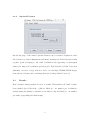
GraspJ User Manual Version 3 Table of Contents Chapter 1 Getting Started ........................................................................ 1 1.1 Installation ......................................................................................................... 1 1.2 Run GraspJ ........................................................................................................ 2 1.3 Run Analysis on Sample Dataset ....................................................................... 2 Chapter 2 Using GraspJ ............................................................................ 3 2.1 Workflows .......................................................................................................... 3 2.2 Workflow Wizard ............................................................................................... 4 2.3 Results ............................................................................................................... 8 Chapter 3 Views ...................................................................................... 10 3.1 Workflow-View .................................................................................................. 10 3.2 Analysis-View .................................................................................................... 12 3.3 Result-View ....................................................................................................... 13 3.4 Settings-View .................................................................................................... 14 Chapter 4 Workflow-Components ........................................................... 15 4.1 Acquisition Config ............................................................................................. 15 4.2 Live Producer .................................................................................................... 16 4.3 Spot Finder JAVA/CL ...................................................................................... 17 4.4 MLE Fitter 2D/3D ............................................................................................ 18 4.5 Fit Filterer ........................................................................................................ 19 4.6 Frame Filterer ................................................................................................... 20 4.7 Trail Generator ................................................................................................. 20 4.8 Package Drift Corrector .................................................................................... 21 4.9 Rendering Config ............................................................................................... 22 4.10 Result/Package Merger ..................................................................................... 23 4.11 Live Renderer .................................................................................................... 23 4.12 Workflow on Copy ............................................................................................ 24 4.13 Continuous Workflow on Copy ......................................................................... 25 4.14 Live Channel-Renderer ...................................................................................... 25 4.15 Injection Producer ............................................................................................. 25 Chapter 5 Troubleshooting...................................................................... 26 ii Chapter 1 Getting Started Please note that GraspJ has only been tested on Windows. However, it should work on Mac OS X and Linux as well if all requirements listed in this chapter are fulfilled. If you experience any problems please contact [email protected] or consider filing an issue on http://code.google.com/p/graspj/issues/. 1.1 Installation The easiest way to install GraspJ is to use the pre-configured Fiji package provided on http://code.google.com/p/graspj/downloads/. It comes with its own Java version and all required libraries. Just download the zip file, and unzip it. Please make sure your computer fulfills all Requirements. It is highly recommended to use a 64bit version and dedicate enough memory to the Java Virtual Machine (JVM), otherwise the analysis might fail or get stuck (see Troubleshooting). Alternatively you can download the plugin as a Java archive (JAR), also available on http://code.google.com/p/graspj/downloads/. For installation this file needs to be copied to the plugins folder of ImageJ/Fiji. Afterwards restart ImageJ/Fiji. This plugin already contains all required dependencies, except Java 7. GraspJ needs Java 7 to run (see Java 7 for more information). 1.1.1 Requirements OpenCL In order to run GraspJ you will need a device that supports OpenCL 1.1 or higher. Among many other devices, most modern Intel and AMD CPUs as well as most modern Nvidia and AMD GPUs support OpenCL. If you have installed a recent GPU driver from Nvidia or AMD, you are most likely already good to go. 1 Details for the main vendors can be found here: • AMD • Nvidia • Intel Java 7 If you have chosen the Fiji package above and are running Windows or Linux, you don’t need to worry about Java 7 as this package already ships with Java 7. Otherwise you will have to install Java 7 manually and make sure ImageJ runs on Java 7. The Java version your ImageJ/Fiji runs on can be checked by clicking on the status bar of ImageJ/Fiji. A version number 1.7.X indicates Java 7 while 1.6.X indicates Java 6. GraspJ needs Java 7 to run. If not already installed, Java 7 can be downloaded here. ImageJ/Fiji has to be running on the Java 7 virtual machine (VM) in order to run GraspJ. 1.2 Run GraspJ Start ImageJ/Fiji then start GraspJ via PluginsGraspJ. 1.3 Run Analysis on Sample Dataset Download the sample dataset and the sample workflow from www.graspj.com. Drag & drop the sample workflow to GraspJ. The workflow will be opened in a Workflow-View. Expand Producers and click on Live Producer. On the right locate the field Source File. Drag & drop the downloaded sample dataset to that field. Then click on WorkflowRun Analysis. 2 Chapter 2 Using GraspJ In order to analyze your own data you need to create a custom workflow. The easiest way to do so is by using the Workflow Wizard. Alternatively you can modify the sample workflow or start with an empty workflow. 2.1 Workflows The analysis procedure of GraspJ is organized in a modular way that we call a workflow. 2.1.1 Create Workflows Workflows can be created in two ways, either by using the Workflow Wizard (FileWorkflow Wizard) or starting from scratch (FileEmpty Workflow). You can also modify existing workflows. 2.1.2 Save/Open Workflows Workflows can be saved while in Workflow-View (also see general description of Views). There are three data-formats available, gjw, gjwx and gjwxz. Those abbreviations stand for GraspJ Workflow, GraspJ Workflow XML and GraspJ Workflow XML zipped, respectively. Workflows saved in gjw format are in a binary format. Workflows saved in gjwx format are text files with XML code to describe the workflow. The gjwxz format is identical to the gjwx format except that the data is zipped to achieve smaller file sizes. Workflows can be opened either by drag & drop onto GraspJ or using a dialog from the menu (FileOpen Workflow). 3 2.1.3 Workflow Phases A Workflow consists of three different phases during which the final result is obtained. Those phases are called Production, Processing and Consumption and the components working during these phases are called Producers, Processors and Consumers, respectively. Available components and their configuration are described in Chapter 4 (Components). During Production phase typically the raw data is read, sliced into pieces of suitable size which we refer to as packages. Those packages will later also store the list of localizations, filtering results, calculated drift and any other information created during Processing. The second phase, Processing, consists of a number of individual components all facilitating parts of the analysis by working with an individual package at a time. Each Processor is called once per package and execution of the subsequent Processor is delayed until the predecessor is finished, maintaining the order of Processing. At the end of this phase the analysis of the individual package is finished. The last phase is called Consumption. Here the package is simultaneously distributed to all consumer-components. Typical examples of consumers are rendering engines providing the user with the obtained image in different ways. 2.2 Workflow Wizard To start the Workflow Wizard click on FileWorkflow Wizard. The Workflow Wizard allows you to choose the data to be analyzed and enter the specifications for the data file (e.g. 2D or 3D, multi- or single-color) and microscope settings (e.g. pixel size). 4 2.2.1 Data Source On the first wizard page you have to choose a method to load your data. If your data is saved as a single file in a raw format (i.e. no header/footer, no gap between images…) you have to choose the first option (Load as Raw Data). This option provides the highest reading speed and can also be used for live-analysis (data can still be written to the file, it does not even have to exist yet). If you choose to open your data this way, you will have to specify the width and height of a single frame in pixels as well as the bytes used to represent a single pixel (e.g. 2 bytes for a 16-bit image). If your data is saved in a format supported by the LOCI Bio-Formats library, the second option can be used to load your data (Load with LOCI Bio-Formats). Depending on the file-format, this option might be substantially slower than the first 5 option. Live-analysis is also supported for many (but not all) formats loaded in this way (there is no list of which ones are supported). If you already opened your data in ImageJ, you can use the third option (Use open Stack). The reading speed will vary, depending on whether it is loaded as a virtual stack. Non-virtual stacks will already be loaded in RAM which makes reading very fast. However, most STORM/PALM stacks are large and will likely be loaded as a virtual stack. If that’s the case, reading speeds will depend on the location of the file. If it is located on a solid-state disk (SSD), speeds will be similar to the rawloading-method. For conventional hard-disks (HDDs) it will be slightly slower and for network locations it will typically be substantially slower. In the latter case using a raw format should be considered. 2.2.2 Analysis Type Config On the second page you have to specify whether your data is 2D or 3D. For 3D data, GraspJ currently only supports astigmatism. In case the data source you specified on the first page is already accessible and consists of enough frames (≥10), GraspJ will try to automatically determine a few pa6 rameters needed for analysis, such as threshold. In order to determine the imaging sequence/cycle that was used during acquisition (for further information see Frame Cycle), you will be asked for the number of different channels/colors GraspJ should expect. The remaining options on that wizard page concern rendering of found localizations. If you activate Render an Image with all Channels an image with all localizations regardless of their color-channel will be rendered together in one window (“bad” renderings are filtered out). The option Render Channels individually lets you specify color-channel numbers that will be rendered in separate windows. Color-channels are assigned to localizations based on the frame in which they occurred (see Frame Cycle). 2.2.3 Basic Configuration The third page lets you specify parameters essential for identification and localization of molecules. GraspJ will try to estimate some of the values itself (currently limited to Threshold and Frame Cycle). Those parameters typically have a big effect on the performance of GraspJ (see Acquisition Config, Spot Finder JAVA/CL, MLE Fitter 2D/3Dfor details on the individual parameters and how to set them properly). 7 2.2.4 Optional Features On the last page of the wizard optional features can be activated. Right now available features are Trail Generation and Drift Correction. Trail Generation links together peaks belonging to the same localization but appearing on subsequent frames (for improved localization precision) (see Trail Generator). Drift Correction (intrinsic) corrects for stage drift in x and y by rendering STORM/PALM images from subsets of frames and correlating them (see Package Drift Corrector). 2.3 Results Data obtained during analysis is saved as results. This includes all found localizations (named Spot-Collection), a (filter-) Mask (i.e. one number per localization, characterizing its channel or whether it was filtered out) and Drift (i.e. one number per frame representing the shift in nm). 8 2.3.1 Save/Open Results Results can be saved while in Result-View (also see general description of Views). They can be opened either by drag & drop onto GraspJ or using a dialog from the menu (FileOpen Result). 9 Chapter 3 Views Views are the central part of GraspJ’s user interface. Everything shown below the menu bar is a view. Each opened view adds an entry to the Views menu which when clicked becomes the active view. Each view-type also adds an entry to the menu bar offering commands that can be used within this view. The WorkflowView as well as the Result-View also contains data that can be saved. For example, if you click on FileSave As while in Workflow-View, the current workflow will be saved. Similarly, if you click on FileSave As while in Result-View, the current result will be saved. All views and their specific commands are explained in this chapter. 3.1 Workflow-View The Workflow-View allows you to view and modify essential parameters of the analysis, including the ones that were entered as part of the “Workflow Wizard”. 10 On the left side the workflow is shown as a tree-structure (see Workflows for more information on what a workflow and its components are). The structure of the workflow can be changed via drag & drop inside the tree. More options are available through the context menu (right-click). If you right-click on a component, you will be presented the option to remove that component. If you right-click on a “folder”, e.g. Processors, you can add an additional Processor by choosing from a list of available Processors. On the right side all options for the selected component inside the tree are shown and can be edited. 3.1.1 Workflow-Commands Run Workflow Starts execution of the current workflow and switches to a new Running-AnalysisView. Add to Favorites This function adds the current workflow to the list of favorite workflows. This list is part of the Result-Commands. To view and modify the list or workflows added to it, click on FileSettings which will lead you to the Settings-View. Attach to Result This function attaches the current workflow to an open result. You will be able to choose the result you want to attach the workflow to in a popup window. Attached workflows can be accessed through the Result-Commands. They are shown and can be edited in Result-View after expanding “Others”. 11 3.2 Analysis-View Analysis-View shows the status of a running analysis, such as the number of localizations found and how many frames have been analyzed. 3.2.1 Analysis-Commands Pause Analysis This command pauses the running analysis. Live-Renderings can still be inspected (zooming/panning). Resume Analysis This command resumes a paused analysis. 12 Stop Analysis This command stops the running analysis (the current package will be finished first). It then proceeds to show the result in a Result-View. 3.3 Result-View The Results-View shows previews of the final rendered images obtained as a result of the analysis as well as additional results such as the amount of drift in x and y. 13 3.3.1 Result-Commands Built-in Workflows Some workflows commonly run on results can be selected from this menu. Attached Workflows Workflows attached to this result can be opened from this menu. The workflows are also shown and can be edited in Result-View after expanding “Others”. Workflows can be attached to results using the Attach to Result command in Workflow-View. Favorite Workflows Your favorite workflows can be opened from this menu. The workflows are also shown and can be edited in Settings-View. Workflows can be added to your favorites using the Add to Favorites command in Workflow-View. 3.4 Settings-View In this view you can change settings used by GraspJ, like the used OpenCL platform and device or your favorite workflows. 14 Chapter 4 Workflow-Components 4.1 Acquisition Config 4.1.1 Pixel Size This is the size of one (projected) camera pixel in nm. Pixels are assumed to be squares. (Example: physical pixel size: 16µm × 16µm, using a 100x objective Pixel Size ≈ 160nm). 4.1.2 Count Conversion This is the factor to convert pixel intensity values to approximate photon counts. This conversion factor depends on the gain settings of the EMCCD camera and should be determined from the provided manufacturer specifications. 4.1.3 Frame Cycle This is the order of frames inside the source file. Enter the repetitive pattern of the acquisition. For each frame of this pattern you need to enter one digit representing the color-channel that frame belongs to. Frames can be marked as activation frames by putting square brackets around them. Example: For a two-color experiment where identical reporter dyes but two different activator dyes are used a typical frame cycle consists of: one activation frame of one color (e.g. Alexa405) followed by three acquisition frames (e.g. Alexa647) followed by one activation frame of a second color (e.g. Cy3) and finally three acquisition frames (e.g. Alexa647). For such a frame cycle, the following pattern would be adequate: [1]199[2]299. The numbers in brackets represent the first and second activation frames, which typically are dark and contain no localizations. The 1 and 2 outside of the brackets indicate the first and second acquisition frames immediately following the activation frame. The 9 identifies non-specific localizations from 15 the frames not immediately following the activation frame. For a detailed reference on multi-color imaging using different activators, please refer to Bates et al, Science, 317: 1749 (2007). 4.2 Live Producer Reads the data source and splits it into packages. The analysis procedure is then done package-wise. 4.2.1 Frames per Package This is the number of frames per one package. Setting this number too high might result in the analysis failing as the package will not fit into the GPU-RAM anymore. Setting this number too low, on the other hand, might result in low analysis speeds or impaired intrinsic drift correction. A typical number of frames per package is 1024. 4.2.2 Data Source Type A detailed description of the options available here can be found in section 2.2.1 (Data Source). 4.2.3 Detect End of Data Source Decides whether the Live Producer will try to automatically detect the end of the acquisition (or in non-live mode the end of the file). If not selected one has to stop the analysis manually (see Running-Analysis-View). Interval The time (in ms) the Live Producer waits between two consecutive attempts to load new frames. 16 Attempts Number of times the Live Producer attempts to load new frames before it stops the analysis. 4.3 Spot Finder JAVA/CL This component is intended for facilitating the peak finding part of the analysis. 4.3.1 Max. Spots per Frame This is the maximum number of peaks the finder will try to find inside a single frame. If this number is set too high the Java version of the Spot Finder will use up a lot of RAM and the CL version might fail due to insufficient GPU RAM available. If this number is set too low not all peaks in a given frame may be found. For a typical STORM/PALM dataset this number can be set to 1024. 4.3.2 Threshold This is the minimum intensity count the brightest pixel of a peak must have to be considered for fitting. This value is critical for analysis. If this number is chosen too high not all peaks will be identified. If it is chosen too low the finder will pick up noise as peaks. This will slow down analysis and Max. Spots per Frame might be exceeded before all peaks are identified, even if the number of actual peaks within a single frame is low enough. GraspJ determines a rough estimate for the threshold from the first few frames of the data. However, the estimate is often not accurate enough to give the best results. Therefore, the user is recommended to open the data in ImageJ and determine the threshold by considering the dimmest peaks in each frame that should be included in the analysis. 4.3.3 Box Radius This is the “Radius” of the box that is drawn around the highest intensity pixel of a peak and is used to exclude overlapping peaks and peaks on the edge of a frame. 17 The size of the square box used corresponds to2 ∗ 𝐵𝐵𝐵 𝑅𝑅𝑅𝑅𝑅𝑅 + 1. As a rule of thumb the box radius should be set to approximately 3 ∗ 𝜎𝑃𝑆𝐹 , where 𝜎𝑃𝑆𝐹 is the Standard Deviation PSF. 4.4 MLE Fitter 2D/3D This component performs the peak fitting part of the analysis. 4.4.1 Box Radius This is the “Radius” of the box that is drawn around the highest intensity pixel of a peak and is used for fitting to obtain its center position. Usually this value should be chosen identical to the Box Radius of the Spot Finder JAVA/CL. 4.4.2 Standard Deviation PSF This is the standard deviation of the Gaussian approximation to the Point-SpreadFunction of your microscope in pixels. 4.4.3 Iterations This is the number of iterations run while fitting each peak. The higher the number the closer the fit result will be to the MLE, but the analysis speed will go down. 4.4.4 Defocusing Curve X/Y (3D only) The z-position of fluorophores is determined based on the astigmatism of the PSF in 3D data. The astigmatism is compared to a calibration curve in order to determine the z-position. The calibration curve must be obtained by immobilizing single fluorophores or fluorescent beads on the surface of a cover glass, and scanning a precision piezo stage in z (for example for a range of +600 to -600 nm). The peaks in this calibration dataset must be identified and the x and y widths of the PSF must be determined in each frame. This analysis allows one to plot a calibration curve (x- and y-widths of the PSF as a function of z-height). This calibration curve 18 can then be fit to a “defocusing” curve to determine the parameters needed for the 3D analysis. For more details on astigmatic 3D super-resolution imaging please refer to Huang et al., Science 319: 810 (2008). More details on the 3D calibration parameters used in GraspJ can be found in Smith et al., Nature Methods, 7: 373 (2010). 4.5 Fit Filterer This component filters “bad” localizations based on certain criteria. 4.5.1 Apply Mask If this option is selected, the obtained filter mask is permanently applied to the Spot-Collection, i.e. bad localizations are deleted. 4.5.2 X, y, z, Intensity, Background For each of those parameters one can specify a lower and upper limit of the value itself as well as the uncertainty of the found value. If the value or the uncertainty is outside of that range, the localization will be filtered out. The cut-off for the localization uncertainty in x, y and z is set in nm (e.g. 30 nm for x and y and 50 nm for z). Localizations with low photon counts and hence large uncertainties will therefore be filtered out. This cut-off can be changed to accept more or less localizations and will affect the final resolution of the image (accepting localizations with high error will degrade resolution. On the other hand, accepting only localizations with very low error may lead to filtering out a large number of localizations and degradation of the image resolution by lowering the Nyquist sampling). The minimum and maximum intensity should be set based on the minimum and maximum number of photons expected from individual molecules. 19 The maximum background value can be used to reject localizations from very crowded regions where close-by fluorophores could have affected localization accuracy. It is not straightforward to find a suitable value that fulfills that task and some trial and error will be needed. However, this value is not very important and if set to a large number no localization will be filtered out because of this number. Bad localizations are still filtered out by the other criteria, especially uncertainty in x and y. 4.6 Frame Filterer This component filters localizations based on the frame in which they appeared. 4.6.1 Apply Mask If this option is selected, the obtained filter mask is permanently applied to the Spot-Collection, i.e. bad localizations are deleted. 4.6.2 Filter by Channel If selected, all localizations that do not belong to specified channel are filtered out. 4.6.3 Filter by Type If selected, all localizations that are not of the selected type (activation/acquisition) are filtered out. 4.6.4 Encode Channel If selected, the channel number, determined from the Frame Cycle, will be saved in the filter mask. 4.7 Trail Generator In a typical STORM/PALM experiment, the acquisition laser intensity is chosen such that individual fluorophores switch-off or bleach within one frame. However, 20 some fluorophores may last longer than one frame. When the same peak appears in multiple frames, it can be trailed together and the position calculated as a weighted average of the positions in each frame. Trailing improves the localization accuracy of a given peak. The trail generator allows you to set up the parameters for linking peaks together. 4.7.1 Location Tolerance This value determines how far the position of two peaks can be separated from one another in subsequent frames to be still considered the same peak. The value is set in nm. 4.7.2 Frame Skip Tolerance This value determines the number of frames that a peak can disappear in between frames to still be considered as the same peak. Typically trailing is done only for peaks that continuously appear in subsequent frames and therefore this value is set to zero. 4.7.3 Min/Max Trail Length This value determines the minimum and maximum number of frames that can be trailed together. Typically this value is set to be equal to the length of the acquisition frames in a cycle (e.g. 3). 4.8 Package Drift Corrector This component corrects for stage drift in x and y by rendering STORM/PALM images from subsets of frames and correlating them (intrinsic drift correction). By default it renders all-channel images for correlation. If you want to restrict the correlation to a specific channel, you can use the Specific Channel setting of the Rendering Config used by the Package Drift Corrector. If you want to use fiduciary 21 markers that appear in a certain frame of your Frame Cycle, you can do so by dedicating an individual number to that frame in the cycle-setup and then choosing the same channel number for the Specific Channel setting. Example: Let’s consider the same situation as discussed in the example given in section 4.1.3 (Frame Cycle), where we had a two-color data set which led to the following cycle-pattern: [1]199[2]299. Now, let’s assume we added fiduciary markers that appear in the otherwise dark activation channel for the second color: [2]. In order to localize the markers in that channel and identify them separately from the single molecules we will have to assign an individual number to that frame, we here choose 3. The cycle-pattern would then become: [1]1993299. Now, by setting the Specific Channel option to 3, the Package Drift Corrector will only use the localization from the fiduciary markers for drift correction. 4.9 Rendering Config This feature allows to set-up the parameters for rendering localizations as an image. 4.9.1 Render Width This is the width of the window in pixels that should be used for the final rendering. 4.9.2 Render Height This is the height of the window in pixels that should be used for the final rendering. 4.9.3 Pixel Size This determines the pixel size in nm at which the image will be rendered. 22 4.9.4 Offset X/Y This determines the shift of the rendering in nm. 4.9.5 Intensity This determines the intensity of the rendering of an individual localization. It’s the sum of all pixel-intensities that belong to that localization. 4.9.6 Apply Mask If selected, the current (filter-) mask is applied during rendering, e.g. localizations that were filtered out are not rendered. Specific Channel This option allows to specifically only render localization that belong to a specific channel (defined by the Channel Nr option) and are not filtered out. Hue and z (ColorCoded3D only) In 3D super-resolution images, the z-height of localizations is color-coded using a continuous color-scale. Hue is calculated from the z location using the following linear transformation formula: ℎ𝑢𝑢(𝑧) = 4.10 ℎ𝑢𝑒max − ℎ𝑢𝑒min ℎ𝑢𝑒max 𝑧min + ℎ𝑢𝑒min 𝑧max 𝑧+ 𝑧max − 𝑧min 𝑧min − 𝑧max Result/Package Merger This component appends the current package to the current result of the workflow. 4.11 Live Renderer This component continuously renders the current result of the workflow. The rendering is shown in a modified ImageJ-Window allowing for zooming, panning etc. 23 4.11.1 Push/Receive Actions When activated, zooming and panning actions on this rendering window will be pushed to/received from all other rendering windows within the same group specified by Group Names. Group Names Specifies the groups this rendering belongs to as a comma separated list. 4.11.2 Auto Contrast This is used to automatically scale the brightness/contrast of the rendered image. The brightest points correspond to those that contain the highest number of localizations. 4.12 Workflow on Copy This component can hold and run a workflow on (a copy of) the current result/current package of a parent workflow. For each package delivered to the component a new workflow will be run. 4.12.1 Copy current Result/Package If selected, the workflow uses a copy of the current result/package of the parent workflow. A copy in this sense refers to a shallow copy, which means that without further configuration the spot-collection, the mask and the drift are still identical to the original ones (i.e. changes made to the result/package on this workflow affect the result/package on the parent workflow). However, the result/package itself is a copy, which means that you can replace the spot-collection/mask/drift with a different one without affecting the parent-workflow result/package. 4.12.2 New Spot-Collection/Mask/Drift If this option is selected the spot-collection/mask/drift is replaced with a new one. 24 Copy original Spots/Mask/Drift If this option is selected, the newly created Spot-Collection/Mask/Drift is filled with a copy of the original data. If you select this option for all three parts (Spots/Mask/Drift), you will end up with a deep-copy of the result/package. Changes to that copy will not affect the original. 4.13 Continuous Workflow on Copy This component is largely identical to Workflow on Copy. The main difference is that, instead of executing a full workflow for each package, it has one workflow running continuously while the parent workflow is running. New packages are then injected into this workflow by the Injection Producer. One application of this component is the Live Channel-Renderer which is based on the Continuous Workflow on Copy component. 4.14 Live Channel-Renderer The main functionality of this component is similar to the Live Renderer (in fact a Live Renderer is built-in to this component). It adds the functionality of filtering a copy of the spot-collection before rendering to allow for rendering of individual color-channels only. This component is based on the Continuous Workflow on Copy component. 4.15 Injection Producer This component replaces the Live Producer in Continuous Workflow on Copy based components. Instead of reading the source file and creating packages for analysis, it uses a copy of the parent-workflow package and injects it into the workflow. 25 Chapter 5 Troubleshooting The analysis stops without any error m essage shown. This can be caused by insufficient memory available to ImageJ/Fiji. If possible, increase the memory ImageJ/Fiji is allowed to use via EditOptionsMemory & ThreadsMaximum Memory, then restart ImageJ/Fiji and try again. It is highly recommended to use a 64bit version of Java7 and the 64bit version of GraspJ. If none of this works you can try setting a smaller number of Frames per Package in the Live Producer configuration. The analysis is very slow. While the analysis is running, check execution times shown in the Analysis-View. If one of those is especially high, check the configuration of that component. If execution times for all components are reasonable, the low speed is most likely caused by a low reading speed of your source file. More information on how to choose the best option for your data source is given in section 2.2.1 (Data Source). Briefly, the fastest reading speeds will be achieved using a raw file format and reading the source file from a fast hard drive (for example a Solid-State Drive (SSD)). Im ageJ/Fiji com plains ab out GraspJ b eing com piled for a newer Java version. This indicates that your ImageJ/Fiji is running of a Java version too low to run GraspJ. Please check the Installation section of this manual for more information. 26