Download Comparing the NDS and VERA environments for scan chain

Comparing
the
NDS and VERA environments
for
scan chain recognition & removal
M. van Balen
Concerns
Period of work
Supervisor
Advisors
:
:
:
:
:
:
End Report
April 1993 - Dec 1993
prof. ir. M.T.M. Segers
ir. F.G.M. BOUWffiall
ir. J.M.C. Jonkheid
ir. P.W.M. Merkus
© Philips Electronics N. V. 1993
All rights are reserved. Reproduction in whole or in part is
prohibited without the written consent of the copyright owner.
M. van Balen
Comparing
the
NDS and VERA environments
for
scan chain recognition & removal
ABSTRACT
To cope with testing problems for large and complex logic circuits it is widely acknowledged
that one has to partition the circuit into independently testable blocks and apply structUIal
Design-For-Testability techniques. A generally adopted Design-For-Testability tec1mique
is scan design. In this case all, or a selected part of, the flip flops in the design are replaced
by a scannable variant. These scannable variants form a shift-register, by which the design
can be set in any desirecl state.
In tlus report algoritluns are clerived for finding and removing such scan-chains. We use
the implementation of these algoritluns as a vellic1e for comparing the NDS and VERA
enviromnents, discussing (dis )advantages of both worlcls.
Keywords : NDS, VERA, OutScan, scan design, design-for-testability
© Plulips ElectrOllics
N.V. 1993
i
Preface
This work was performed in partial fulfillment of the requirements to become Master of
Electrical Engineering at the Eindhoven University of Teclmology. It was performed at
the Philips Research Laboratories in Eindhoven dming the period april- december 1993.
Acknowledgernents
First of all, I would like to thank my mentors Paul Merkus, Johan Jonkheid, and Frank
Bouwman of the Philips ED&T group for their enthusiastic support. I also want to thank
Krijn Kuiper, Steven Oostdijk, Hans Bouwmeester, and the other members of the group
for their valuable help regarding my work and this report. F'tuthermore I thank my fellow
students, Ruud van der Meer and Frank van de Voort, for the many fruitful discussions
concerning om projects, and their pleasant company dming my work at Philips.
Finally I want to thank prof.ir. M. T .M. Segers for being my supervising professor, and
for giving me the opportunity to carry out tlus project in lus group.
Philips Research Laboratories,
Eindhoven, December 7, 1993
Martijn van Balen
© Plulips ElectrOlucs
N.V. 1993
111
Contents
1 Introduction
1
2 The design and test of integrated circuits
3
3
4
2.1
IC design
3
2.2
IC testing
6
2.2.1
7
Structure testing
Scan test
9
3.1
Design for testability .
9
3.2
Introduction to scan test.
10
3.3
Advantages and disadvantages of scan test .
12
Hierarchical, logic circuits
15
4.1
15
Cells
.
4.1.1
Leaf cells
16
4.1.2
Non-leaf cells
16
4.2
Ports.
16
4.3
Nets
16
4.3.1
4.4
ltlstaJlces
17
Asynchronous and syncluonous sequential circuit
18
4.4.1
Asynchronous circuits
18
4.4.2
Syncluonous circuits .
19
4.5
Clock ports of a syncluonous cell
19
4.6
Functionality of cells . . . . . . .
20
4.6.1
Functionality of leaf cells
21
4.6.2
Functionality of non-leaf cells
21
4.6.3
Circuit models . . . . . . . .
21
© Philips ElectrOlllcs
N.V. 1993
v
5
6
A structural model of hierarchical circuits
23
5.1
Ports, and the set of ports
23
5.2
Instanees of a set of cells .
24
5.3
Port references of a set of cells
24
5.4
Nets of a set of cells
24
5.5
Cells, and sets of cells
25
5.6
Descendence . . . .
26
5.7
Descendent graph .
27
5.8
Terminology. . . .
31
5.9
An example of a design
31
A functional model of synchronous cells
35
6.1
Values and time . . . .
35
6.2
Internal state of a cell
36
6.3
Fllllctionality of a cell
36
6.3.1
Fllllctionality of an output port of a cell
36
6.3.2
Combinatorial and sequential output ports
36
6.4
7
A structural model of scan chains
7.1
8
9
37
Determining the functionality of non-Ieaf cells
39
Scan chain definition and reality . . . . . . . . . . . . . . . . . . . . . . .. 42
FindScan: the algorithm
43
8.1
Restrictions on clock ports .
43
8.2
Restrictions on enable ports
44
8.3
Example of a FindScan session
45
RemoveScan: the algorithm
49
9.1
RemoveScan for leaf scan chains
49
9.1.1
Examples of leaf cells
49
9.1.2
Automatic match-rule generation for combinatorial cells
51
10 The NDS environment
VI
55
10.1 NDS classes
55
10.2 LDS classes
56
© Philips
Electronics N.V. 1993
11 SDS
57
.
57
11.1.1 The SDS object hierarcllY
58
11.1.2 Relation between SDS and NDS classes
58
11.1.3 The RoutingPlan class
59
11.1.4 The Macro class
59
11.1 SDS classes
'"
11.1.5 The ClockDomain class
60
11.1.6 The ClockPin class
60
11.1. 7 The Chain clas s
60
11.2 The RoutingPlan Language
61
12 VERA
63
12.1 hltroduction
.
63
12.2 Rules, matches, and actions
64
12.2.1 The "test" rule .
65
12.2.2 The "path" rule
65
12.3 ND: the Network Descriptionlanguage .
66
12.4 TD: the Type Descriptionlanguage . . .
67
13 NDS: implementation of the algorithms
69
13.1 FindScan
.
69
13.1.1 File formats.
69
13.1.2 hlformation flow
69
13.1.3 Generating of the leaf scan chains file with GenRpI .
69
13.1.4 Tracer
73
13.2 RemoveScan.
73
13.2.1 File formats.
73
13.2.2 hlformation flow
73
13.2.3 Generating the match-rule file .
73
14 VERA: implementation of the algorithms
14.1 FindScan
©
77
.
77
14.1.1 File formats.
77
14.1.2 hlforlnation flow
77
14.1.3 Generation a leaf scan chains file
77
Philips Electronics N.V. 1993
vii
14.1.4 Rpl2TD
.
78
14.1.5 Match-rules used to recognise scan chains
79
14.1.6 Determining the scan chains of a design
82
15 Comparing NDS and VERA
85
15.1 Design manipulation .
85
15.2 Implementation effort
86
15.3 Run-time and memory requirements
86
1504 Reliability
87
15.5 Flexibility
87
16 Possible improvements
89
16.1 Extension of the scan chain definition
16.2 Strueture versus expressions
89
.
89
16.2.1 Implementing RemoveScan using expressions
90
16.2.2 Automatic generation of the Match-rule file
90
17 Conclusions
91
A Mathematical notation
95
A.1 Abbreviations.
95
A.2 Sets anel tuples
95
A.3 Predefined sets
95
AA Operators . . .
96
B The Routing Plan Language
99
B.1 Syntax ..
99
B.2 Semantics
101
B.3 Semantic rules
101
B.3.1
102
Rules regarcling uniqueness
B.3.2 Rules regarcling order of definition
B.3.3
. 102
Rules regarcling length of chains
102
B.3A Rules related to the design
B.3.5
VUl
Other rules
102
.
103
© Philips Electronics
N.V. 1993
List of Figures
4
2.1
The IC design and test trajectory .
3.1
The canon.ica1111ode1 of a circuit
.
11
3.2
The canonica1111ode1 of a sCaJmab1e circuit.
11
4.1
The cell as a black box
.
15
4.2
Exalllp1e of a design without Ïllstances
17
4.3
Exalllp1e of a design with instances . .
17
4.4
Structure of an asynchronous sequentia1 circuit
18
4.5
Canonica1 structure of a synchronous sequentia1 circuit .
19
5.1
The tennino1ogy useel by different 1anguages .
31
5.2
Exalllp1e of a circuit: COUNT
.....
33
5.3
Descendent graph of circuit "COUNT" .
34
8.1
A descenelence graph ..
44
8.2
The FindScan a1gorit1ull
46
8.3
A cell containing scan cllains
47
9.1
Rep1acelllent of an inverter
50
9.2
Rep1acement of a buffer ..
50
9.3
Rep1acelllent of a D flipflop
50
9.4
Rep1acelllent of a lllultip1exer
51
9.5
Rep1acelllent of a sCallllab1e D flipflop
51
9.6
The RellloveScan a1goritlun
.
53
.
58
11.2 Re1ations between SDS alld NDS classes
59
11.1 Ownership of SDS objects
© Philips E1ectrOlllcs N.V.
1993
ix
x
12.1 Syntax of the VERA test rule .
65
12.2 Syntax of the VERA path rule .
66
12.3 ND: the VERA netlist fonllat .
67
12.4 TD: the VERA type descriptioll format
67
13.1 Information flow during a FilldScan session
70
13.2 Information flow during aRemoveScan session
74
14.1 Information flow during a FindScan session
78
14.2 The VERA batch file generated by Rpl2TD
79
14.3 A type containing two separate chains . . .
81
15.1 Run-time results in seconds of FindScan on a HP9000/735 platform
86
© Philips
Electronics N.V. 1993
Chapter 1
Introduction
Testing ofIntegrated Circuits (ICs) has become a major issue in research and development
of Very Large Scale Integration (VLSI). ICs have been growing continuously innumber of
transistors and complexity. This has caused an increase in the probability of both design
errors and manufactming faults. Manufactming faults result in defects on the IC, while
design errors result in an lUldesired fUIlctionalïty of the chip. To prevent design errors,
the design must be checked at several stages of the design. It is not possible to prevent
manufactming faults, in fact, the yield is typically between 40 and 80 percent. Because the
market asks for reliable, zero defect ICs, every single IC produced must pass several tests.
One of these tests is the structme test. The idea of structme test is that all structures,
created on the silicon slUJace, must be tested for correctness. The problem of structure
testing of ICs is complicated by the enormous amolUlt of possible faults, and the limited
accessibility of parts of the ICs via the IC pins.
The requirements for a structure test are strict. The test should be fast because it is perfOl'llled on every individual IC, and it must still have a high fault coverage since customers
do not accept faulty ICs. FUI'thenllore, it is important that we are able to generate this
test in a short time in order to prevent lengthy design times. It is generally believed that
these requirements can only be met if already during the design phase the IC testability
is taken into account. This is referred to as design for testability (DFT).
There are many DFT tec1miques. hl general, they operate by improving the controllability
and observability of the circuit. This means that test patterns can be transported more
easily to isolated parts of the IC and the responses can be more easily captured. Generating
test patterns becOlues less complex and the fault coverage increases. The DFT technique
that we are concenled with in this report is scan test.
Scan test is a DFT method that improves the testability of a design drastically by creating
an extra 'test' operation mode for the design. hl normalmode, the design operates just as
it is supposed to, according to its specification. hl test mode, the memoryelements will
all be connected into one or more scan paths. To do this, all memoryelements must be
replaced by versions that are equipped with such a test mode (we will call such aversion
the scannable variant). A scan path is a shift register that is only active during test mode.
Through this scan path test patterns can be applied to the rest of the circuit, that now
only contains combinatoriallogic. After applying a test pattern during normal mode, the
©
Philips ElectrOlllcs N.V. 1993
1
responses can be captured at the primary outputs and the inputs of the memory elements.
The captured responses in the memoryelements can then be shifted out during test mode
and gathered by the tester. In this way, test pattern generation has only to be done for the
combinatorial part of the circuit, thus easing the process of structure testing very much.
This report deals with the specification and implementation of FindScan and RemoveScan.
FindScan identifies scan c1lains in a design, while RemoveScan is able to remove this
extra scan fUllctionality from a design. The algoritluns have been implemented using two
different environments, NDS and VERA.
This report comprises the following activities: First agIobal introduction to the testing
of les is given, followed by a discussing of scan test. Then models are given to be able
to describe circuits and scan chains in a formalmanner. This is followed by a description of the two algoritluns and their implementations. Finally the two envirOlunellts are
compared, discussing their (dis )advantages for scan chain recognitioll and removal.
2
© Philips
ElectrOlucs N.V. 1993
Chapter 2
The design and test of integrated
circuits
Before an IC can be delivered to a customer, its correctness must be determined. This
implies that each individual IC must operate conform to its specifications. Since the design
of ICs is done in a llllluber of phases, it must be checked that for each phase no errors are
introduced (an error meaning a difference between implementation and specification). In
this chapter we will fust discuss the IC design process in more detail. Secondly, we will
take a look at the IC testing process, which is closely related to the design process.
2.1
IC design
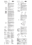
In an IC design trajeetory we distinguish several phases [Woudsma90J. They range from
requirelllent specification via fllllction specification and structme specification to finally
the layout. The layout is used in the lllanufactmillg process to make the IC. These phases
are depicted on the left hand side of figure 2.1.
Below, we describe the design phases that are mentioned in figure 2.1.
Requirement specification: First an informal description of au IC will be drawn up,
using a natmal language, specifying the desired requirements. This specification
describes both what the IC should do, formulated in behaviomal tenns (the fllllCtion behaviour), and under which conditions (e.g., environmental aud parametric
constraints ).
Funetion specification: The requirement specification is transformed into a fUlletion
specification. Here one specifies what the arclliteetme of an IC would be and which
fUlletions it should perform. AIso, the necessary top levellllodules and their interactions are determined. This specification is formal. One could, for instance, think
of a VHDL description of a design being the funetion specification.
Strueture specification: The fUlletion specification is then trausformed into a structme
specification. In this phase the modules aud intercomlections resulting from the
funetion specification are worked out in more detail to the level of basic building
©
Philips Eleetronics N.V. 1993
3
û~IBm~î~p~f~~~i~~lr----1.Ç~"t%11~J
1I
.• .•:.:•.:•.:.: .: '.: .,:.
II6.l.·.•·.:·..........:::::::::~~Î:q,~#:::::::
.
:.:-:-:-:.;.:.:.:.:.:.:.:.;.;««.:.:.:.:.:.:::;::::.::::::::::::::::::
1 -..... . . .
,..-
I
~:~:.·.~l~• ~~io.~h~]~tk~:·• ~ t.·:~: : ~: :~: ~.: :.: :.:·.:V
"
;>-f.,""":
~•.•.•: .: :.••.:.:.•:. :.•.•.•:.•
.:
;.;.;.; :.:.;.:.:.:.:.;.:.:.:.:.;.;.:.:.:.:.:
design trajeetory
: ·.r:
•.•., '
test trajeetory
Production
Figure 2.1: The IC design and test trajectory
4
@ Philips Electron.ics N. V. 1993
blocks from the library. This models the electrical connectivity. An example of this
specification is an EDIF netlist description of a design.
Layout: The structure specification is then transformed into a layout. This specifies the
placement of the different building blocks, and maps these block and their interconnectioIlS to polygons, describing the topology of the chip area. An example of this
specification is GDS Ir.
Product: The layout is used to actually manufacture the IC in a f01llldry.
The trajectory of creating an IC is very complex and highly error prone. Therefore, one
has to take precautions to guarantee that each delivered IC conforms to its specification.
To accomplish this, verification is used during the design trajectory, and testing is used
during the test trajectory (after production of the IC).
To clarify the distinction between verification and testing, we will discuss them below:
Verification: Comparing the results of two successive phases with each other is called
verification. It is denoted by the upwards pointing arrows in the design trajectory in
figure 2.1. hl this figure two verification steps are denoted by dotted arrows. These
verification steps can be done, but, they must be performed by hand.
During the design trajectory, a higher-level description was transformed in a lowerlevel description. To verify whether tlus step was perfonlled correct, the opposite
action is taken. That is, given the lower-Ievel description, a lugher-Ievel description
is extracted.
Tlus extracted lugher-Ievel description is then compared with the lugher-Ievel description used during the design trajectory. Inconsistencies indicate errors.
For instance, a composition of transistors can be transformed into a composition of
logic AND and OR gates by means of verification. Tlus can then be compared to
the gate level description that was aheady present tlus level in the design stage.
The advantages of verification is that it can be done prior to the manufacturing of
the clup, and more importantly it doesn't need any stimuli, hence it is exhaustive.
Testing: When the layout of a design is created, the chip can be produced. During the
production process, a substantial part of the ICs will become defect. Therefore,
eacll individual IC must be cllecked to see if it operates according to its specification. During testing, certain stimuli are presented to the input pins of the IC and
responses at the outputs are collected and cllecked against the expected behaviour.
An advantage of testing is that it can be done for all design stages, which can be
seen in the right hand side of figure 1, where the test trajectory is depicted. Disadvantages are that testing can only be done after the IC is manufactured, and that
it cannot be done exhaustively (for large ICs). This is because an exhaustive test
means that we should test all possible states of an IC, and for every state we have
to test all possible input combinations. For an IC with N flip flops and Pinputs
tlus means that we have to test 2N + P different states. If there are only 50 flip flops
and 10 inputs, testing tlus very small clup at 100 Mhz would aheady take about 350
years ....
© Plulips ElectrOlucs
N.V. 1993
5
2.2
IC testing
Since IC production yields are typically between 40% and 80%, tests should be applied to
every IC produced, in order to meet quality requirements. Therefore, the IC design phases
are followed by extensive testing. This testing can also be divided into several phases. In
general we can state that every phase in the design trajectory has an equivalent phase in
the test trajectory [Beenker 90, Claasen 89], see also figure 2.1.
Each test phase has a different goal, but they all have in comlllon that they increase the
confidence one has about the IC being manufactured according to the original specification.
The following test phases are depicted on the right hand sight of figure 2.1:
Layout testing: Layout testing is not done very extensively. This originates from the
fact that matching a layout with the specification is practically not possible at this
moment. What can be (and is) done is checking if all layout masks were correctly
aligned when producing the chip. This checking can be easily done right after production by checking if certain markers, that were present on each mask, are well
aligned on the chip.
Strueture testing: Structure tests look for defects that result in an incorrect behaviour
and are caused by the IC production process. It should be applied on every IC
produced, because each single IC may contain structural faults. This is the maill
reason that for structure testing limitation of the test time is very important.
In the trade-off between test time and the possibility of all incorrect IC passing the
test, normally a (high) number of test patterns are applied. These test patterns
are generated by a test pattern generator according to certain fault models. Fault
models are used to define the meaning of "fault". Many real faults can be modeled by
faults defined by such a fault model, but generally they willnever cover all possible
faults.
Examples of fault models are the stuck-at, and the bridging-fault fault model.
Structure test (only) requires knowledge of the structure. This implies that test
patterns can be generated automatically, based upon a chosen fault model.
Funetion testing: Test patterns for function testing are usually produced by the designer of the IC. They include tests at the critical ends of the function specification,
and will normally only be applied to a few samples of the ICs produced, because
structure testing should already have proven that the IC structure corresponds with
the structure specification. Hence, this kind is only needed to assure that the ICs
produced are in conformity with the function requlrement.
Sometimes structure testing is not enough to prove the correctness of the structure. In those cases, function testing is performed on every sample, to increase the
confidence one has in the testing trajectory.
Function test requires the knowledge of the function of the design. This implies that
the designer most produce the test patterns.
Application mode testing: In this test the IC is installed in an application environment, or software is used to model such an enviromnent. This test examÏnes the
6
©
Philips ElectrOlllcs N.V. 1993
correetness of the IC design in its application and such proves that the IC is suitable
for such an application.
Also, a characterisation test can now be perfonlled. This test aims at varying the
performance of the circuit lUlder varying environlllental and electrical conditions
(for example temperature, voltage and llluuidity). During this phase the actual
electrical specification of the circuit can be detenllÎned. Charaeterisation is also
called "performance testing".
Application mode testing requires knowledge of the application. One has to know
the specific application to bllild it, or to be able to simulate it.
The area of interest to us in tlus thesis is structure testing. Therefore, we look at tlus
kind of testing more closely in the following section.
2.2.1
Strueture testing
The large density of modern circuits results in an enormous amount of possible fault cases.
The maill problem in structure testing is the question how to detect such faults, given the
limited accessibility via the IC pins.
A naive, but straightforward, strategy for structure testing is exhaustive testing. Here all
possible test patterns are applied and the responses are collected. These responses can
then be compared to the expected responses. The major drawback of tlus method is that
for larger circuits the test would take so much time that it is not suitable for practical
purposes. Especially for strllcture testing tlus is uuacceptable, because the structure test
must be applied to every IC produced.
hl the case of circuits contaitl.Îng memory elements, i.e., sequential circuits, the problem
is even worse. For these circuits the output not only dep end on the input but also on
the current state of the circuit. hl order to test a sequential circuit exhaustively, one has
to traverse all internal states of the circuit and for each state all test patterns should be
applied.
The illtractability of the exhaustive test strategy has led to a search for other, practically
more useful, strategies. The next chapter will give an introduetion to scan test, one of the
strategies that can be used to ease struetllre testing.
© Plulips ElectrOlucs N.V.
1993
7
Chapter 3
Scan test
The previous chapter showed that it was virtually impossible to perform exhaustive structUI'e tests on large sequential designs. This was due to the fact that a lot of test patterns
are needed to traverse all internal states of a circuit. FUI'thermore, the problem remained
of how to access structUI'es on the chip via the input pins. These facts result in increasing
test complexity, which can be converted into costs associated with the testing process,
such as the cost of test pattenl generation, the cost of test equipment, and the cost related to the testing process itself, namely the time required to detect and/ or isolate a
fault. Because these costs can be high (and may even exceed design costs), it is important
that they be kept within reasonable bounds. One way to accomplish this is by the process
of design for testability (DFT).
3.1
Design for testability
Testability has been defined in the following way [Bennets 84J:
An electronic circuit is testable if test-patterns can be generated, evaluated,
and applied in such a way as to satisfy predefined levels of performance (e.g.
detection, location, application) witlun a pry-defined cost budget and time
scale.
Design for testability (DFT) can then be described as the design effort that is specifica1ly
employed to enSUI'e that a device is testable.
There are two important attributes related to testability, namely controllability and observability. Controllability is the ability to establish aspecific signal value at each node in
a circuit by setting values on the circuit's inputs. Observability is the ability to determine
the signal value at any node in a circuit by controlling the circuit's inputs and observing
its outputs.
StructUI'e testing mainly involves applying test patterns to the circuit that we are testing,
and then observing the responses. Hno specific DFT technique is used, the entire circuit
can only be controlled through its input pins. Tt may be clear that for a large design
(thousands of gates, or more) the controllability will soon become very poor, since the
© Plulips ElectrOlucs N.V. 1993
9
number of input pins is restricted (no more than several tens or hUlldreds) and structures
on the IC may be fairly isolated (not directly accessible from the input pins). Also, the
observability will become very poor because of the same reasons and the restricted nUlllber
of output pins. The poor controllability and observability makes the process of creating
test patterns very difficult. This may become so hard that it is not possible anymore to get
a high fault coverage within reasonable time and costs. At this point the decisionmust be
made to accept a lower fault coverage or apply DFT teclmiques to increase controllability
and observability. Since a lower fault coverage often is not acceptable, the choice then
falls on DFT .
There are a n1llllber of DFT techniques. Most of them deal with either the re-synthesis
of an existing design or the addition of extra hardware to the design. This means that
they affect such factors as chip area, 1/0 pins, and circuit delay. Hence, a critical balance
exists between the amount of DFT to use and the gain achieved. Test engineers and
design engineers usually disagree about the amOlUlt of DFT hardware to include in a
design. In this report, we will focus only on the DFT technique that is of importance to
us, namely scan test. The remainder of this chapter contains all introduction to scan test,
and discusses the arg1llllents for and against it.
3.2
Introduction to scan test
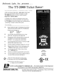
One of the most popular structured DFT techniques is referred to as scan design [Fujiwara 85]. The classical Huffman model of a (synchronous) sequential circuit is shown in
figure 3.1. In this canonical model the memoryelements (registers) are separated from the
rest of the circuit, so that the remaining part of the circuit is combinatorial. The combinatoriallogic has a n1llllber of primary inputs (PI) and a n1llllber of secondary inputs (SI,
the outputs of the registers). The output of the combinatoriallogic consists of primary
outputs (PO) and secondary outputs (inputs to the registers). Since the tot al circuit is
sequential, testing it may be complicated if the circuit is large.
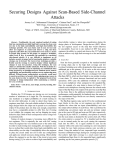
hl figure 3.2 the scan version of the circuit is shown. The registers are now replaced by
scan registers. A scan register is a register that can operate in two modes. In the normal
mode, it acts as a normal register, just as the ones that were used in figure 3.1. hl test
mode, the scan register will clock its data in from the 'scan-in' input instead of its normal
data input. After the clock pulse, this data will be present on the 'scan-out' output. The
'test' input detennines the mode in which the scan register will operate. Hence, a scan
register has tluee special pins associated with it besides the original pins of a register,
namely the 'scan-in', the 'scan-out' and the 'test' pin.
The scan registers cannow be transformed into one or more scan paths, by cOlUlecting the
'scan-out' pin of one scan register with the 'scan-in' pin of the next scan register. This
means that the registers now form a shift register when put in test mode. In figure 3 this
is illustrated.
Testing has now become much more easier. Since all memoryelements can be easily
controlled and observed via the scan path (in test mode) the inputs and outputs of scan
registers can be treated as primary inputs and outputs of the combinatoriallogic.
This means that we are able to shift test patterns in the scan path and apply them to
10
© Philips
ElectrOlllcs N.V. 1993
Inputs
.-
Combinatorial
circuit
~
:
Outputs
I---
f--
Registers
.............................1.......................,...............
Clock
Figme 3.1: The canonîcal model of a circuit
:
:
Inputs
r-
Combinatorial
circuit
~
Outputs
-
:
:
ScanIn
:
Registers
ScanOut
l............................ .1......... 1............................,
Clock
Test
Figme 3.2: The canonical model of a scanllable circuit
@ Philips Electronics N.V. 1993
11
the combinatoriallogic. The outputs of the combinatoriallogic can be captured at the
primary outputs of the circuit and at the inputs of the scan registers. Instead of perforIlI..ing
a sequential test on the entire circuit, it llOW suffices to perform a combinatorial test on
the combinatoriallogic, together with a test to check that the shift register is operating
correctly. These two tests are much easier and faster to generate than the sequential test.
AIso, the fault coverage willnormally be better.
Testing a scan design in this way will be referred to as scan test in this report.
3.3
Advantages and disadvantages of scan test
One ntight tltink that scan test is the preferred solutioll for testing a (complex) sequential
circuit when reading the previous section. Tltis is however not always true. There are a
number of costs to be observed when using scan test. [Benllets 93] gives an overview of the
arguments for and against scan test. Below, we give a smllillary of some solid argmllents
used by [Benllets 931.
Advantages of scan test:
• Test pattern generation for the combinatorial parts of the circuit can be done
fully automated. Furthermore, the pattern generation software will always find
a test for a fault if there is one. Popular test pattern generation algOritlUlls for
combinatorial circuits indude Podem [Goel 81] and Fan [Fujiwara 831.
• The fault-simulation costs are lower because the fault simulator is needed only
for the combinatorial parts of the circuit. The fault coverage should be 100
• The design debug capabilities by using scan paths to explore the behaviour of
the intended circuit are better.
• The design environment stays manageable because of the existence of design
tools and rule checkers. AIso, there is a strong belief that scan enforces wellbehaved dock schemes. Such schemes can reduce tinting problems in the fulal
design. The fulal benefit of a controlled design envirOllIDent is lower risk of a
major design change (= quicker time to market ).
• The ability to locate the cause of a defect has increased because of the partitiOlting through the scan path.
Disadvantages of scan test:
• Scan test introduces extra silicon and pins. Pins cost money, especially if the
need for scan causes an increase in package size. In case pins are the most
expensive, it 's possible to use existing pins, in exchange for some extra controller
area on the chip.
• Scan memoryelements are usually enhanced versions of regular memory elements. The enhancement is normally done by adding a multiplexer fmlction to
the front end of the memory element. Tltis extra functionality can be seen to
increase propagation delays hence the potential impact on performance. There
are ways to avoid tltis problem, but the preferred way is that the design library
is enhanced to contain dedicated scan cells.
12
© Philips Electronics
N.V. 1993
For a more complete discussion of these topics, the reader is referred to [BelUlets 93].
Tt may be clear that the designer has to weigh these arguments agaînst each otller to decide
whether or not he should use scan test for lus design. In general, it can be stated that
when extra silicon, pins and delays are not critical factors, there are no serious reasons why
the designer should not choose for scan test. When one or more are critical, the designer
should see if the problem can be worked arOlllld in some way, because the advalltages of
using scan test are clear. Partial scan, as discussed in [Voort 93], is a way of reducing the
costs that come with scan test, and may therefore be very interesting to the designer.
© Plulips ElectrOlucs N.V.
1993
13
Chapter 4
Hierarchical, logic circuits
In tlus ehapter we will diseuss the term circuit. A circuit, also referred to as system, or
design, is a eollection of cells. The behaviOlll' of the eells is sueh, that the circuit performs
a required task.
4.1
eells
A celt ean be seen as a black box, processing the information carried by its inputs to
produce its output (see figure 4.1). These input and output cOImections are called the
ports of the eell. The way in wluch the inputs are processed to produce the outputs is
called the behaviour of the cello
Cell
Inputs
Outputs
Figure 4.1: The cell as a black box
Depending on the level of abstraction, port values may be voltages, logic values, data
words, etc. These values are also time dependent. In tlus paper we will use the logic
abstractionlevel, i.e., ports are considered to carry (time dependent) logic values.
Whell tillung relations are ignored, and only value transformation is considered, we speak
of the logic function of a cello The logic function is represented by the functional model of
that cello Time does play a role in such a model, but it will be abstracted.
Besides describing a cell by its function model, we can also specify the function of a eell
by using a structural model. Use tlus model, a cell is a box, containing a collection of
interconllected smaller boxes, called elements, or children. These elements in their turn
may also be modeled by interconllection of lower-Ievel cells. TlJ.is reslllts in a hierarchical
© Plulips
ElectrOlucs N.V. 1993
15
circuit, in which cells are continuously described in tenns of lower-Ievel cells, Ulltil cells
are reached which are described by a fUllction model.
When a cell C contains an element which refers to another cell C 2 , we say that cell C
cOlltains an instanee of C 2 • The internal intercollnection of C will specify how its elements
are interconnected, and how the ports of Care cOlUlected to these elements. Since these
elements actually refer to other (lower-Ievel) cells, they do not own ports, but the cells to
which they refer do. So interconnecting will be described using the ports of C, and the
port referenees of its (lower-Ievel) elements.
4.1.1
Leaf eells
A Zeaf eelt is a cell which is not described in term of lower-Ievel cells, but contains functiollality "by definition". These built-in properties / attributes are logic fUllctions, which
are described using a fUllction model.
4.1.2
Non-Ieaf eells
A non-Zeaf eelt is a cell that does contains children, i.e., it is described using a structural
model.
4.2
Ports
Ports of a (leaf or non-Ieaf) cell represent the interface to and from the external world.
They are electrical connectors which can be cOlUlected to otller ports, or to some external
world source/destination. Using the direction of infonnation flow, we distinguish four
types of ports:
input ports: InforIllation flow is always directed from a higher-level cell to lower level
cell(s).
output ports: Illformation flow is always directed from a lower-Ievel cell to higher level
cell(s ).
inoutput ports: Information flow can be directed from a higher-level cell to lower level
cell( s), or vice versa.
undireeted ports: hûormation flow direction is not specified, and must be derived by
examination of the structural specification.
4.3
Nets
Nets are used to model the intercOlUlections. All ports and port references of such a net
are electrically cOlmected, i.e., they form a "galvanic unity". At all arbitrary point in
time, these ports and port references carry the same value, the value of the net.
16
© Philips Electronics N.V.
1993
4.3.1
Instanees
Gne could wonder why a non-leaf cell contains elements which refer to other cells, instead of
just containing those otller cells. The advantage of the fust approach, i.e., using instaI1CeS
of cells, can be clarified by looking at the following example:
Suppose a designer has to design a fom-input AND, having two-input NANDs aIld inverters
leaf-cells as building blocks. This CaIl be done with three two-input NANDs aIld tlrree
inverters. The designer however will think in term of building the fom-input AND with
tlrree two-input ANDs, wh.ich in their tmn CaIl be build up using a two-input NAND with
an inverter. This approach is depicted in figme 4.2 .
...
,...............................................
,
,
.
.
J
Op
Figme 4.2: EXaInple of a design without instaI1CeS
With instances, the designer can fust build an two-input AND, using a two-input NAND
and an inverter. Then he CaIl use tlrree different instanees of this AND, to construct the
desired fom-input AND. This approach is depicted in figme 4.3.
:.,:::::...-:::....
,
.,:1
:.10.
:...·~iï;i··········
-
.
I
~.. :-. =-. :-. :-. :-.. :-. :.I
.
~
Figme 4.3: Example of a design with instances
It looks like the only thing that has ChaIlged is that the tlrree NAND /inverter combinations
have got a box drawn aroUlld them. But the major difference is the fact that the tlrree
boxes have the same naIue: AND2. Aftel' AND2 is constructed, we can use it to construct
a higher-level cell (in this case AND4), using the leaf-cells and the AND2 cello
Ir cells would contain other cells directly, every cell could be "instaIltiated" only once.
In case of figme 4.2, every NAND used would be a separate leaf-cell, with no explicit or
implicit relation to the otller NANDs. They would each have their own fUllction specification.
Another advaIltage of using instaI1CeS in the formal structmal model is the fact that
the practical environments which aI'e used, i.e., NDS aIld VERA, also use the instaI1Ce
concept. Transforming algoritlullS, which are written using the formal models, into aIl
implementation is therefore rather straightforward.
© Philips ElectrOlllcs N.V.
1993
17
4.4
Asynchronous and synchronous sequential circuit
Sequential circuits contain memory. This implies that the value of an output port at a
certain time, may not only be detennined by the input port values at that time, but
also by the state of the memory elements. The values stored in these memoryelements
determine the internal state of the cello Since cells are finite, they will also have a finite
number of possible internal states.
Based upon the way in which the memory is realised, we distinguish asynchronous, and
synchronous circuits.
4.4.1
Asynchronous circuits
An asynchronous circuit contains feedback between combinatorial inputs and outputs,
shown in figme 4.4. Because of this, a change of value of an input port at an arbitrary
point of time, may result in a change of the internal state of the circuit. Tt is even possible
that by such an input value change the internal state of such a circuit will never be stabIe,
1llltil the input values have changed again.
Since the designing of an asynchronous circuit involves less restrictions than designing a
synchronous circuit, realising a f1lllction using asynchronous circuits will almost certainly
result in a smaller (never a larger) layout. The major drawback of an such a circuit
however, is the fact that its behaviom heavily depends on the delay between input and
output changes of cells. This not only makes allalysis of these circuits much harder, but
also complicates the testing process.
This report focusses on scan chains, which can be seen as subcircuits fOUlld in synchronous
circuits. From now on, we will only discuss synchronous circuit in this report .
..........................................................................
.:
.:
.
:
Inputs :
r
~
Combinatorial
circuit
: Outputs
f---f--
1
:
J
I
Figme 4.4: Structure of an asynchronous sequential circuit
18
©
Philips Electronics N.V. 1993
4.4.2
Synchronous circuits
In case of a synchronous circuit special memoryelements are used. Such a memory element
is docked by a synchronous dock. This doek generates so called doek pulses, which divide
time into time slots, starting at t = tI, t2, t3, ... Events at time tI, t2, t3 ... are initiated by
dock pulses on the dock lines.
Each time a dock pulse is received, the input values are sampled, and the next internal
state and the output values are detennined. Both are a function of the sampled inputs
and the current state.
Because the memoryelements can now be separated from the combinatoriallogic, we can
consider an arbitrary sequential circuit to have a eanonieal structure of the form showed
in figure 4.5.
In this picture, the dock lines of the memoryelements are directly cOlUlected to input
ports. It is however possible that the doek lines of the duImen of a cell, are driven by
input ports, through combinatoriallogic. Tlus logic canllot be part of the "normallogic"
of the cell, since tlus would violate the restrictions (iI'awn upon synchronous circuits,
resulting in an asynchronous circuit.
,- - _
····
-- . -
_
_
-
-·····-t
...
:
:
Inputs :
:
:
,.....".
r--
Combinatorial
circuit
: Outputs
-
Memory
Cloek inputs
:
:
tÎ
Figure 4.5: CanOlucal structure of asynchronous sequential circuit
4.5
Cloek ports of a synehronous eell
We can distinglush several kinds of sequential devices, all docked in a different ways:
Pulse-triggered: hlput values are sampled during the '1' (or '0') period of the dock
port. Output values change during tlus same period.
© Plulips
ElectrOlucs N.V. 1993
19
Edge-triggered: Input values are sampled just before the rising (or falling) edge of the
doek port. Output values change just after this edge.
Master-Slave: Input values are sampled just before the rising (or falling) edge of the
doek port. Output values change just after the next, falling (or rising), edge. Some
master-slave flip flops have separate doek-ports: one for the master part, and one
for the slave-part.
Pulse triggered flip flops caImot be used in scan ehains, sinee during one aetive doek period,
data ean be propagated through more than one flipflop. With sueh a configuration, its
impossible to put eaeh scan flipflop into a desired state.
The other two flip flops ean be used in scan ehains. After sampling its input values at
a doek-edge, the master-slave flipflop ehaIlges its output value(s) at the next, opposite
type, edge. Sinee this is before the next input-sample edge, it eaIl be modeled by an
edge-triggered flipflop. In case of master-slave flip flops with separate master, and slave
doek-lines, we must use the master cloek-line, sinee it detenuines the input sample time.
Definition 4.1: [doek pulse] A doek pulse is a change of value on a doek port. We
distinguish two kinds of doek ports, denoted by their polarisation:
Positively polarised: A doek pulse is a 0 to 1 traIlsition. Events oeeur on the rising
edge of this doek port.
N egatively polarised: A doek pulse is alto 0 transition. Events oeeur on the falling
edge of this doek port.
o
In this modeling of doek ports we have associated a positive (negative) polarity with a
rising (falling) edge. This assoeiation is arbitrary ehosen, we eould just as well haven
ehosen to swap the meaning of positive and negative.
When a eell is doeked by more than one doek port, we will assume that their doek pulses
will always oeeur at the same moments in time. We then ean think of sueh a set of doek
port as being "the doek" of that eell. N ote that this is a different interpretation of multiple
doek lines than the master-slave flipflop with separate master and slave dock-lines.
4.6
Funetionality of eells
The functionality of a eell is in faet the eollection of the funetionality of all its output
ports. The functionality of sueh a port ean be described by a boolean funetion, deseribing
the value on sueh a port at a eertain point in time, depending on the input port values
and the eurrent internal state of the eell.
We ean distinguish two kinds of output ports:
Combinatorial: The output port value does not depend on the internal state of the eell.
Sequential: The output port value does depend on the internal state of the eell.
20
© Philips
Electronies N.V. 1993
4.6.1
Funetionality of leaf eells
Leaf eells eontain funetionality "by definition", i.e., for every output port, the function is
specified by a boolean fllletion.
4.6.2
Funetionality of non-leaf eells
Non-Ieaf eells eontain instanees of lower-Ievel eells. Suppose the funetionality of these
lower-Ievel eells is knOWIl. Beeause the referenees to the ports of these lower-Ievel eells are
eODnected to nets of the parent, the functionality of the lower-Ievel eells specifies arelation
between values on the nets of the parent eell.
Combining all relations between net-values specified by the ehildren, llsing the connection
between ports of the parent and those nets, result in the functional deseription of the
parent eell. This functional deseription uses the Uluon of all internal states of the cluldrell.
Tlus Uluon ean been seen as the internal state of the parent eell.
We have assUlned that the functionality of the clulch'en eells was knOWIl. Tlus is not
a restriction. Sinee the lowest-Ievel non-Ieaf eells OlUY use instanees of leaf eells, the
functionality of the parent ean be deternuned. Aftel' tlus, the eells wlueh use instanees of
leaf eells, and instanees of the just proeessed lowest-Ievel non-Ieaf eells, ean be processed.
Tlus ean be eontinued Ulltil all eells are processed.
4.6.3
Circuit models
In the next ehapter we will discuss a structural model for circuits. A circuit will be modeled
by a set of eells, in wlueh a eellmay llse instanees of otller eells. Leaf eells are eells wlueh
have no c1uldren, and no nets. Non-Ieaf eells eontain cluldI'en, wlueh are intereonnected
by a set of nets. Tlus model will be used to fonnally define the concept of "scan ehains".
© Plulips ElectrOlues
N.V. 1993
21
Chapter 5
A structural model of hierarchical
circuits
In order to be able to recognise scan cllains in a given circuit, we'll have to define precisely
what is meant by "scan chain". Since a scan chain is a part of a circuit, we fust have to
define what we mean by "circuit".
In this chapter we will define a model, with whicll we can formally describe the structure of
a circuit. Using the Edif tenninology, a structuralmodel for multiple instance, hierarchical
circuits is given. This enables the reader who is falluliar with Edif terms, to use an intuitive
interpretation of these terms.
5.1
Ports, and the set of ports
Definition 5.1: [set of ports] The set of ports (denoted by PO RT) is defined as the set
wluch contains all port~. A port is a basic entity wluch will be used as a base for further
defuutions.
o
Definition 5.2: [set of directions] The set of directions (denoted by DIR) is defuled
by
DI R
= {input, output, inout, undirected}
o
Definition 5.3: [direct ion of a port] The direction of a port (denoted by dir) is a
relation on PO RT, defuled by
dir: PORT
--t
DIR
o
Definition 5.4: [input ports] The set of input ports (denoted by I PO RT) is defuled by
IPORT
= {p E PORTldir(p) E {input,inout}}
© Philips Electronics N.V.
1993
23
o
Definition 5.5: [output ports] The set of output ports (denoted by 0 PO RT) is defilled
by
OPORT = {p E PORTldir(p) E {output,inout}}
o
5.2
Instanees of a set of eells
The definition of a set of instanees is relative to a set of eens. The definition of a set of
eens will be given later on, sinee it depends on several definitions whieh depend on the
definition of set of eens.
Definition 5.6: [set of instanees] Let C ELL be a set of eens. The set of instanees
(denoted by INST) is a relation on CELL. INSTcELL is the set which eontains all
instanees of C ELL. An instanee is a basie entity whieh will be used as a base for further
defillitions.
o
Definition 5.7: [instanee] I is an instanee of a set of eens C ELL, iff I E IN STCELL.
o
5.3
Port referenees of a set of eells
Definition 5.8: [set of port references] Let C ELL be a set of eens. The set of port
references (denoted by PO RTREFcELd is a relation on IN STCELL is defilled by
PORTREFcELL = INSTcELL X PORT,
with tuple element nalnes (I, P).
o
Definition 5.9: [port of a port reference] Let CELL be a set of eens. The port of a
port reference (denoted by port) is a relation on PORTREFcELL defilled by
port: PORTREFcELL
---t
PORT
o
5.4
Nets of a set of eells
Definition 5.10: [set of nets] Let C ELL be a set of eens. The set of nets (denoted
by N ETcELL) is a relation on C ELLdefined by
NET = P(PORT X PORTREF),
24
© Philips
Eleetronies N.V. 1993
with tuple element names (P, P R), where:
Vn E NET: In.PI
+ In.P RI
E 1N+
o
Definition 5.11: [net] n is a net iff n E NET
o
A net n is a tuple, containing a finite set of ports, and a finite set of port references. At
least one of these sets is non-empty.
5.5
eells, and sets of eells
In this seetion we will define the declaration eell of an instanee, a set of eells, and the
descendent relation(s) on a set of cells. Since these definitions are mutually dependent , we
have to use forward references, i.e., references to objeets which haven't been defined yet.
Definition 5.12: [declaration eell of an instanee] Let CELL be a set of cells. The
declaration eell of an instanee (denoted eelt) is a relation on l N STCELL defined by
eell: l N STCELL
---+
C ELL,
with C ELL the set of cells, which will be defined next.
o
Definition 5.13: [set of eells] A set of eells C ELL is defuled by
CELL = P(PORT)
X
P(lN STCELL )
X
P(N ETcELL) ,
with tuple element names (P, l, N), where
• All ports of a cell of C ELL must be a member of exactly one net of that cello
VC E CELL: (Vp E C.P: (:JIn E C.N: p E n.P))
• All port references of a cell of C ELL must be a member of exactly one net of that
cello
VC E CELL: (Vi E C.l: (Vp E eell(i).P: (:JIn E C.N: (i,p) E n.PR)))
• All ports used in a net of a cell of C ELL must be ports of that cello
VC E CELL: (Vp E (C.N).P: p E C.P)
• Each port reference used in a cell of C ELL CüntalllS a port an an instance. This
port must be a port of the dec1aration cell of this instance.
VC E CELL: (V(i,p) E (C.N).PR: p E eell(i).P)
© Philips EleetrOlllcs N.V.
1993
25
• All port referellces used in a net of a cell of C ELL must refer to instances of that
cello
VC E CELL: (V(i,p) E (C.N).PR: iE C.l)
• Ports may only be part of one cello
VC, C' E C ELL: C
=1=
C'
=}
C.P n C'.P =
0
• histances may only be part of one cello
VC, C' E C ELL: C
=1=
C'
=}
C.l n C'.l
=0
• A cell may not (indirectly) use an instance of itself. This is defined using the descendence relation, which will be definition next.
VC E CELL: C
+
~
C
o
Definition 5.14: [cell] C is a celt iff there exists a set of cells C ELL such that C E
CELL.
o
5.6
Descendence
k
Definition 5.15: [kth descendent, k ~ 0] kth descendent (denoted by Ç) is arelation
on CEL L defined by
k
ç: CELL
X
CELL
--+
lB,
where for C, C" E C ELL:
o
C" ç C
k+l
C" ç C
C" = C,
and,
k
:JC' E CELL: (:Ji E C'.l: C" = celt(i)) 1\ C' ç C
1
Let C, C' E C ELL. Ir C' ç C holds we say an instance of C' is used in cell C. Ir C'
holds for same n > 1 then there exist n - 1 otlier cells
n
ç C
such that
26
© Philips
ElectrOlllcs N.V. 1993
o
* is a relation on
Definition 5.16: [descendent] The descendent relation (denoted by Ç)
CEL L defined by
* CELL
ç:
X
CELL
--+
IB,
where for C, C" E CELL:
*
k
C' ç C == 3k E IN: C' ç C
The descendent relation is thus the refiexive and transitive closure of the kth descendant
relation.
o
+
Definition 5.17: [true descendent] The true descendentrelation (denoted by Ç) is a
relation on CEL L defined by
+
ç:
CELL
X
CELL
--+
IB,
where for C,C" E CELL:
+
k
C' ç C == 3k E IN+: C' ç C
The true descendent relation is thus the transitive closure of the kth descendant relation.
o
5.7
Descendent graph
Definition 5.18: [descent graph] The descent graph of a set of cells C ELL (denoted
by GCELL) is defined by
GCELL
= P(CELL) X
P(CELL
X
CELL),
with tuple element names (V,E) (vertices, and edges), where
V
= CELL
1
Ä
VC,C' E CELL: (C,C') E E == C' ç C
o
Theorem 5.1 Let CELL be a set of cells. The descendence graph
acyclic graph (DAG).
Proof: Suppose
© Philips
GCELL
GCELL
is a directed
contains a cycle, i.e. there is a n E IN, such that
ElectrOlllcs N.V. 1993
27
and
Henee
+
CÇC
But C
!l+ C
for eaeh C E C ELL, so we ean eonclude that
GCELL
is acyclic.
Definition 5.19: [port set of a een] Let C ELL be a set of eells. The port set of a eelt
(denoted by P) is a relation on C ELL defilled by
P: CELL
->
P(PORT)
where:
'<IC E CELL: P(C) = C.P
D
This relation ean be used to retrieve the set of ports of a eell.
Definition 5.20: [input port set of a een] Let C ELL be a set of eells. The input port
set of a eelt (denoted by lP) is a relation on CE LL defilled by
lP: CELL
->
P(PORT)
where:
'<IC E CELL: IP(C)
= P(C) nIPORT
D
This relation ean be used to retrieve the set of input ports of a eell.
Definition 5.21: [output port set of a een] Let C ELL be a set of eells. The output
port set of a eell (denoted by 0 P) is a relation on C ELL defilled by
OP: CELL
->
P(PORT)
where:
'<IC E CELL: OP(C) = P(C) nIPORT
D
This relation ean be used to retrieve the set of output ports of a eell.
28
© Philips
Electronics N.V. 1993
Definition 5.22: [port referenee set of a een] Let CELL be a set of cells. The port
referenee set of a eell (denoted by P R) is a relation on C ELL defined by
PR: CELL
~
P(PORTREF)
where:
VC E CELL: PR(C)
= ((i,p) E PORTREF!i E C.I I\p E P(eell(i))}
o
This relation can be used to retrieve the set of port references of a cello
Definition 5.23: [input port referenee set of a een] Let CELL be a set of cells. The
input port referenee set of a eell (denoted by I P R) is a relation on CEL L defined by
~
IPR: CELL
P(PORTREF)
where:
VC E CELL: IPR(C)
= PR(C) n {(i,p) E PORTREF\p E IPORT}
o
This relation can be used to retrieve the set of input port references of a cello
Definition 5 .24: [output port referenee set of a een] Let CE LL be a set of cells.
The output port referenee set of a eell (denoted by OPR) is a relation on CELL defined
by
OPR: CELL
~
P(PORTREF)
where:
VC E CELL: OPR(C)
= PR(C) n {(i,p) E PORTREFlp E OPORT}
o
This relation can be used to retrieve the set of output port references of a cello
Definition 5.25: [Ieaf een] Let CELL be a set of cells. Leaf eell (denoted by leaJ) is a
relation on CE LL defined by
leaf: CELL
~
IB,
where:
VC E CELL: leaf(C)
== C.I
=0
A cell for which this relation holds, is called a leaf eell. If this relation doesn't hold for a
cell its called a non-leaf eell.
@ Philips ElectrOlucs N.V. 1993
29
o
Definition 5.26: [conneetion] Let CELL be a set ofeells, and CE CELL. Connection
(denoted by 1c) is a relation on P( C) defined by
1C: P(C) X P(C) ~ 1B,
where for p,p' E P(C):
1C(P,P') == :ln E C.N: p E nAp' E n
o
Definition 5.27: [net of a port] Let C ELL be a set of eells, and C E C ELL. Net of a
port (denoted by netc) is a relation on P( C) defined by
netc : P(C) ~ NET,
where for p E P(C):
netc(p)
= {p'
E P(C)11c(P,P')}
o
Definition 5.28: [usage of a port] Let C be a eell, n E C.N. The usage of a port
p E n.P (denoted by used(p)) is a relation on P( C), defined by
usedc: P(C) ~ lB
where for p E n.P:
used(p)
==
(:lp' E n.P: dir(p)
=f
dir(p')) V (:lpr E n.PR: dir(p)
= dir(pr.P))
Sa if pis an input port, usedc(p) holds iff there exists a port whieh reads from the net (i.e.
an output port, or an input port referenee). If p is all output port, usedc (p) holds iff there
exists a port which writes to the net (i.e. an input port, or an output port referenee).
o
Definition 5.29: [usage of a port reference] Let C ELL be a set of eells, CinC ELL,
and n E C.N. The usage of a port referenee pr E n.PR (denoted by used(pr)) is arelation
on PORT REFcELL, defined by
usedc: PORTREFcELL
~
lB
where for pr E n.P R:
used(pr)
== (:lp
E
n.P: dir(p) = dir(pr.P)) V (:lpr' E n.P R: dir(pr)
=f
dir(pr'))
Sa if pr is an input port referenee, usedc(pr) holds iff there exists a port which writes to
the net (i.e. an input port, or an output port referenee). If pr is an output port referenee,
usedc(pr) holds iff there exists a port whieh reads from the net (i.e. an output port, or
an input port referenee).
o
30
© Philips Electron.ies
N.V. 1993
5.8
Terminology
In the model presented here, we use tenns like ceil, port, etc. Unfortunately there exist many different datastructures and languages which are used to describe designs. To
describe a certain construction, they use different terms for the same objects.
In this report we will use our model, the Edif, NDL, and VERA TD /ND lallguages, as
weil as the NDS /LDS datastructures. In figure 5.1 an overview is givell of the termillology
used by all these languages.
Formalmo~
Set of ceils
Ceil
Instance
Port
Port reference
Net
Edif
Design
Ceil
Instance
Port
PortRef
Net
=:J
VERA TD ~NDL
(the file)
(the file)
Type
Macro
Element
implicit
Terminal
implicit
implicit
implicit
Node
implicit
NDSjLDS
Design
Dec1aration Block
Instantiation Block
Dec1aration Port
Instantiation Port
Net
Figure 5.1: The tenllinology used by different languages
5.9
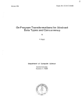
An example of a design
In figure 5.2 an example of a circuit is given. It can be describes using the "set of ceils"
model. Let C ELL denote this set of ceils.
C ELL consists of seven ceils:
CELL
= {INV, NAND, MUX,DFF, BUF, SFF, COUNT}
IN STCELL consists of eight instances. Each instance refers to a ceil, denoted by the cell
relation:
SFF
DFF
BUF
NAND
cell(inst1)
cell(inst2)
ce II (inst3)
cell(inst4)
cell( inst5)
cell(inst6)
cell(inst7)
cell(inst8)
MUX
SFF
INV
BUF
There are four leaf ceils, INV, NAND, MUX and DFF:
INV
NAND
MUX
DFF
({A, Q}, 0, 0)
({A,B,Q}, 0,0)
({A, B, S, Q}, 0, 0)
({D, Cl, Q}, 0, 0)
© Philips Electronics
N.V. 1993
31
The structure of the three non-Ieaf cells is given by:
BUF
=
( {A,Q},
{inst7, inst8},
{
({A}, {(inst7, A)}),
(0, {( inst7, Q), (inst8, A)}),
({Q}, {(inst8,Q)})
}
SFF
=
( {D, DT, SE, Cl, Q},
{inst5, inst6},
{
({D}, {(inst5,B)}),
({DT}, {(inst5,A)}),
({SE}, {(inst5,S)}),
(0, {( inst5, Q), (inst6, D)}),
({Cl}, {(inst6,Cl}),
({Q}, {(inst6, Q})
}
COUNT
=
( {DT, SE, Cl, QO, Q1},
{instl, inst2, inst3, inst4},
{
n1,n2,n3,n4,n5,n6,n7
}
)
)
with
= (0, {(instl,D),(inst4,Q)})
= ({DT}, {(instl,DT)})
= ({SE}, {(instl, SE)})
= ({ QO}, {(inst1, Q), (inst2, D), (inst4, A)})
= ({Q1}, {(inst2,Q),(inst4,B)})
= ({Cl}, {(inst1, Cl), (inst3, A)})
= (0, {( inst2, Cl), (inst3, Q)})
n1
n2
n3
n4
n5
n6
n7
In figure 5.3 the descendent graph of the circuit of figure 5.2 is given. The tluee descendence relations map to the following graph relations:
k
C' ç C
C' ç* C
C'
+
ç
C
means: a directed path of length k exists from C to C'
means: C
= C', or a direeted path exists from C
to C'
means: a directed path exists from C to C'
From this graph it's easy to verify that, among oUler, the following descendent relations
32
© Philips
Electronics N.V. 1993
Cl
inst3
COUNT
BUF
~Q
nl
.---
v
D
DT
n2 inT
SE
n3
A - -n7
instl
inst2
SFF
DFF
n4
Q
D
n5
Q
QI
SE
inst4
'---
NAND
A
Q
QO
B
Cl
inst6
DT
D
SFF
DFF
Q
inst7
inst8
INV
A
Q
.- A
BUF
INV
Q r---- A
Qr
Q
D
SE
D
Cl
DFF
NV
A
Q
Q
S
Figure 5.2: Example of a circuit: COUNT
© Philips Electronics
N.V. 1993
33
hold:
fNV
DFF
1
C
1
C
BUF
SFF
2
DFF C COUNT
DFF c+ COUNT
8
\~
BG
/ t
t
8888
Figure 5.3: Descendent graph of circuit "COUNT"
34
© Philips
Electronics N.V. 1993
Chapter 6
A functional model of
synchronous cells
6.1
Values and time
We will associated a port, a net, or a port reference with a value:
Definition 6.1: [set of values] The set of values (denoted by V AL) is defilled by
VAL
= {0,1}
o
Definition 6.2: [value] v is a value Hf v E V AL.
o
We Oll.1y use the values '0', and '1'. This prohibits the modeling ofbuses, where ports must
be able not to interfere with the bus to which they are conllected, i.e., write the value 'Z'
(high-impedant). Also wired-or, and wired-and constructions calillot be described.
Since we do not intent to describes buses, or wired-or/and constructions, we don't need
the value 'Z'. Also the values 'X' (don't care) alld 'U' (unknown) are not used, since we
don't need them for scan chain recognition.
Definition 6.3: [value on a port] Let pEPORT. The value carried by port pat some
point in time t (denoted by I/(p, t)) is defined by
11:
PORT
X
IN
-7
VAL
o
Definition 6.4: [value on a net] Let CELL be a set of cells, and nE N ETcELL. The
value carried by net n at some point in time t (denoted by v( n, t)) is defined by
11:
N ETcELL
X
IN
-7
V AL
o
© Philips Electroll.ics N.V. 1993
35
Time is modeled by an integer, i.e., time is divided iuto time slots. This suffices for
syuchrouous logic circuits.
Wheu describing combiuatoriallogic, an output port value ouly depeuds on the input port
values, so we can muit time t, and denote the value on a port by 1/( op).
6.2
Internal state of a eell
Since there will be a finite set of memory elemeuts, a cell C will have a finite set of states
iu which it cau beo We cau therefore associate each state with a llluque naturaluumber.
Definition 6.5: [(internal) state of a eell] Let C ELL be a set of cells, and C E C ELL.
The (internal) state of C (deuoted state) is a relatiou on C and the time t defined by
state: C ELL
X
IN
--t
IN
o
Let CELL be a set of cells, CE CELL, aud denote
theu:
state( C, t
+ 1) =
fe( state( C, t), I/(iPl, t), 1/( iP2' t), ... , v(iPIIP(C)I' t))
6.3
Funetionality of a eell
6.3.1
Funetionality of an output port of a eell
In general, the value of au output port, iu time slot t + 1, is a function of the input port
values in time slot t, aud the iuternal state iu time slot t.
Let CELL be a set of cells, CE CELL, aud agaiu deuote
theu:
v( op, t + 1) = fop ( state( C, t), v(iPb t), v(iP2' t), ... , v(iPIIP(C)I' t))
6.3.2
Combinatorial and sequential output ports
Definition 6.6: [eombinatorial] Let CELL be a set ofcells, CE CELL. Combinatorial
(denoted by comb) is a relation on 0 P( C) defined by
comb: 0 P( C)
36
--t
18
© Philips Electrorucs
N.V. 1993
where for op E OP(C):
comb(op) == Vst,st' E STATE(C): fop(st, ...)
= fop(st', ...)
D
This means that the output port value of a combinatorial output port does not depend on
the internal state of its eell, only on its input port values. This implies that the response
to input value changes is not time-dependent.
Definition 6.7: [sequential] Let CELL be aset ofeells, CE CELL. sequential(denoted
by seq) is a relation on 0 P( C) defined by
seq: OP(C)
-t
JE
where for op E OP(C):
seq( op) == -,comb( op)
D
This means that the output port value of a sequential output port does dep end on the
internal state of its eell, not only on its input port values. This implies that the response
to input port value changes is time-dependent.
6.4
Determining the funetionality of non-Ieaf eells
This was aheady (informally) described in a previous ehapter. We must transform the
fmlctions of lower-Ievel eells into fmletions operating on nets of the parent, using the
parents internal state. Then we solve this set of equations and rewrite them using the
ne te relation.
© Philips Electronics
N.V. 1993
37
Chapter 7
A structural model of scan chains
In this chapter we will give a defillition of scan chains. All defillitions are related to a set
of cells. To prevent the use of several "Let C ELL be a set of cells", we will assume from
110won that a set of cells is chosen, and will denote this set of cells by CEL L.
Definition 7.1: [set of enable ports] The set of enable ports (denoted by EN ABLE)
is defilled by
EN ABLE
= IPORT
X IB,
with tuple element names (P, V AL).
o
Definition 7.2: [enable port] eis an enable port iff e E EN ABLE.
o
Definition 7.3: [set of doek ports] The set of doek ports (denoted by CLOCK) is
defilled by
CLOCK
= IPORT X IB
with tuple element names (P, POL).
o
Definition 7.4: [doek port] e is all cloek port iff e E C LOC K.
o
Definition 7.5: [set of ehain elements] The set of ehain elements (denoted by C HAl N EL)
is defilled as the set which contains all ehain elements. A chain element is a basic entity
which will be used as a base for further defillitions.
o
Definition 7.6: [doek port] el is a chain element iff el E CH AlN EL.
o
© Philips
Electron..ics N.V. 1993
39
Definition 7.7: [position of a chain element] The position of a chain element (denoted
by pos) is a relation on C H AINEL defilled by
pos: C H AlN E L ---. IN,
o
Definition 7.8: [instance of a chain element] The instance of a chain element (denoted by inst) is a relation on C H AlN EL defillecl by
ehain: C H AlN EL ---. IN STCELL,
o
Definition 7.9: [chain of a chain element] The ehain of a chain element (denoted
by chain) is a relation on C H AlN E L clefillecl by
ehain: CHAINEL---.CHAIN,
where for el E C H AlNEL:
ehain( el) E C H AINCell(inst(el))
In this clefillition we've usecl CH AINc (with CE CELL). CH AINc will be clefined later
on. The restriction states that a ehain element must refer to a ehain, whieh is part of the
eell to whieh the instanee of that ehain element refers.
o
Definition 7.10: [set of scan chains] Let C E C ELL. The set of sean chains of C
(denotecl by C H AlNc) is clefinecl by
CH AINc
=
IP(C)
X
OP(C)
X
JE
xP(EN ABLE) X P(CLOCK)
xP(CH AlN EL) X IN,
with tuple element nallles (I, 0,1NV, E, C, EL, n).
For all C H E C H AlNc the following holcls:
• (CH.E).P ç IP(C) \ {CH.I}
• (CH.C).P ç IP(C) \ {CH.I}
• (CH.E).pn (CH.C).P = 0
• Ve,e'ECH.E: e.P=e'.P~e.VAL=e'.VAL
• Ve,e' E CH.C: c.P = e'.P ~ c.POL = e',POL
• va ~ i < ICH.ELI:
40
(3 1 el E CH.EL: pos(el) = i)
© Philips
Eleetrollies N.V. 1993
• Let el E CH.EL. We define:
SI(el)
SO( el)
eli
=
=
=
In case CH.EL
(in8t(el),ehain(el).I)
(in8t( el), ehain( el).O)
the element el E CH.EL, for which pos(el)
=10,
=i
the following holds:
- ,c(1, SI(elo))
- ,c(O , SO(ellcH.ELI-l))
- 'VO < i < ICH.ELI- 1: ,c(SO(eli-l),SI(eli))
- CH.INV = EBO.s; i < ICH.ELI: ehain(eli).INV
- CH.n
= 2::0.s; i < ICH.ELI:
ehain(eli).n
- For all en E CLOCKN ET(CH):
('Vel E CH.C: lI(netc(el.P))
('Vel E CH.C: lJ(netc(el.P))
= val(el.POL)) '* v(en.N) = val(en.POL)
= val(el.POL)) '* v(en.N) = val(en.POL)
- For all en EEN ABLEN ET(CH):
('Ven E CH.E: lJ(netc(en.P))
= en.VAL) '* v(en.N) = en.VAL
In tlus defuution we have llsed the set of clocknets and the set of enable nets of chain C H,
CLOCK N ET(CH) and EN ABLEN ET(CH). These sets will be defuled later.
D
Definition 7.11: [scan chain] eh is a scan chain iff there is aCE CELL, for wluch
eh E CH AIN(C).
D
Definition 7.12: [set ofclocknets ofa chain] Let C E CELL, andCH E CHAIN(C).
The set of elocknets of C H (denoted by C LOC K N ET( C H)) is a relation on C H AlN (C)
defuled by:
CLOCKNET:
CHAIN(C)~P(C.NxIB)
with tllple element names (N, PO L), where:
CLOCK N ET(C)
= {(n,p) E C.N
X
1B13el E CH.EL: fc(el, (n,p))}
with
fc(el,cn) _ 3c E chain(el).C: (inst(el),c.P) E (cn.N).PRl\e.POL = en.POL
D
Definition 7.13: [set of enablenets of a chain] Let C E CELL, and C H E CH AIN(C).
The set of enablenetsofCH (denoted by EN ABLEN ET(C H))is a relation on CH AIN(C)
defuled by:
EN ABLEN ET: CH AIN(C)
© Philips ElectrOlucs N.V.
1993
~
P(C.N X V AL)
41
with tuple element names (N, V AL), where:
ENABLENET(C) = {(n,v) E C.N X lBl:Jel E CH.EL: fe(el,(n,v))}
with
fe(el, en)
:Je E ehain(el).E: (inst(el), e.P) E (en.N).PR
À
e.VAL = en.V AL
o
A scan chain eh of ce11 C consists of the fo11owing:
• eh.!: the scan input port
• eh.O: the scan output port
• eh.!NV: a boolean, f alse indicates a non-inverting chain, true illdicates an inverting
chaill.
• eh.E: the set of enable ports, with their enable value
• eh.C: the set of dock ports, with their relative polarity
• eh.EL: the set of chain elements, which concatenated form the chain eh. hl case
this set is empty,
• eh. n: the length of this chain, specifying the ll11mber of dock cydes needed to shift
data from the scan input to the scan output.
Definition 7.14: [leaf scan chain] Let C E CELL.
leafehainc) is a relation on C H AIN( C) defilled by
leafehainc: CHAIN(C)
-t
Leaf scan ehain (denoted by
lB
where:
=0
VCH E CHAIN(C): leafehainc(CH) == CH.EL
o
7.1
Scan chain definition and reality
The theory is suitable to described scan chains which contain only inverters and/ or buffers
in their enable- or dock lines.
42
© Philips Electronics
N.V. 1993
Chapter 8
FindScan: the algorithm
In this ehapter we will give a deseription of FindSeau, au algoritlun eapab1e of 10eating
scan ehain in a eell. In this ehapter we will assume that CE LL is a set of eells.
Scan ehains of 1eaf eells are specified by definition, they ean be eonsidered aheady "ealeulated". When the ehains of an arbitrary eell C E CELL should be ea1eulated, we fu'st
have to ea1eulate the ehains of its ehi1dren. This ean be visualised by inspection of the
decendenee graph of a set of eells.
In figure 8.1 a decendenee graph of a set of eells is given. Prom this picture we eonc1ude
that eells A,B,C,D,E,F are 1eaf eells (they do not instantiate other eells). Therefore the
scan ehains of eell G, H or Jean be ealculated. In order to calculate the chains of eell
K, we have to proeess eells G and H fust. Sinee these restrictions only state the order in
whieh pairs of eells should be proeessed, there remain severa1 valid processing sequenees.
If the eells are proeessed in sueh an order, that it complies with the above restriction, we
ean assume the following, without 10ss of generality: when processing eell C E C ELL, the
c11ains of its c1u1dren are know.
8.1
Restrietions on clock ports
Let C E C ELL be a eell, and C H E C H AI N( C) be a non-1eaf ehain. This implies the
following: for all en E C LOC K N ET( C H):
(Ve
(Ve
E CH.C: v(netc(e.P))
= val(e.POL))
~
E CH.C: I/(netc(e.P))
= val(e.POL))
~
v(en.N)
v(en.N)
= val(en.POL)
= val(cn.POL)
Several (sub )eireuits ean be though of w1ueh satisfy these re1ations. The most obvious one
is to use inverters and buffers to establish the restriction. To detennine the c10ek ports of
a ehain, given its e1ements, our a1goritlun traverses chains of inverters and buffers.
© P1ulips ElectrOlues N.V.
1993
43
(]
\~
88 0
/! !
I\
888888
Figure 8.1: A deseendenee graph
8.2
Restrietions on enable ports
Let C E CELL be a eeil, and CH E CHAIN(C) be a non-Ieaf ehain. This implies the
foilowing: for ail en EEN ABLEN ET(CH):
('ie E CH.E: v(netc(e.P))
= e.VAL) =>
v(en.N)
= en.V AL)
In this case also, several (sub )cireuits ean be though of wh.ich satisfy this relation. Again
we have restricted the algorithm to reeognition of inverter jbuffer ehains.
Definition 8.1: [subehain] Let C be a eeil.
by SU BC H AlN(C)) is defined by
SUBCHAIN(C) = C.N
X
C.N
X
JE
X
The set of subchains of C (denoted
P(ENABLE)
X
P(CLOCK)
X
P(CHAINEL)
with tuple element names (I,O,INV,E,C,EL,n).
All restrietions drawn upon a scan chain apply to a subchain.
D
However, is this case I
=
° is possible, this in the so-eailed null-chain:
(n,n,false,0,0,0,O), nE C.N
The nuil-ehain merely consists of one single net. lts stands for the obvious statement:
"when net n earries a value at time t, net n earries that vahle at time t".
Definition 8.2: [set of scanchains of a subchain] Let C be a eeil, and SC E
SU BC H AIN( C). The set of scanchains of a subchain (denoted by scanchainc) is defined
44
© Philips
Electronics N.V. 1993
X
IN
by
scanchainc: SUBCHAIN(C)
--+
P(CHAIN(C))
where:
scanchainc(SC)
= {CH
E CH AIN(C)I
CH.I E (SC.I).P f\ CH.O E (SC.O).P f\
CH.E = SC.E f\ CH.C = SC.C f\
CH.EL = SC.EL f\ CH.n = SC.n}
o
Thus the set scanchainc( C H) is not empty iff net SC.I contalllS an input port of C, anel
net SC.O contains an output port of C. It will contain more than one chain if net SC.O
contains more than one output port.
In figure 8.2 the FinelScan algoritlun is given. Knowing the scan chains of the children of
a cen C, the chains of C itself will be determined.
8.3
Example of a FindScan session
In figure 8.3 an example cen is given.
cen C contains six instances: two inverters (INV), two multiplexers (MUX), one D flipflop
(DFF), anel one scan flipflop (SFF). All of these children contain scan chains:
CHAIN(C)
INV
MUX
DFF
SFF
{(A, Q, true, 0, 0, 0,on
{(A, Q, false, {(S, On, 0,0,0), (B, Q, false, {(S, In, 0, 0, on
{(D, Q, false, 0, {Cl, true}, 0, In
{(DT, Q, false, {(SE, I)}, {Cl, true}, 0, I)}
When FindScan is executed on cen C, it starts at the net of an output port, in this case
net nI2, which is cOlUlected to port Q. FindScan starts with the fonowing null-chain:
(nI2, nI2, false, 0, 0, 0, 0)
1. Net nI2 is driven by (inst4, Q), where inst4 is a SFF. cen SFF has one chain which
ends at Q:
(DT, Q, faL~e, {(SE, In,{Cl, true}, 0,1)
Since (inst4,Cl) is driven by port Cl, and port en2 drives (inst4,SE) through an
inverter, the subchain now becomes:
(nlO, nI2, false, {( en2, On, {Cl, true}, {elI}, 1)
© Philips Electronics N.V. 1993
45
Coneatenate(S, s)
{
let S' f - 0
foran sE S
{
let ELf- {el E C HAl NEL I ::lel' E s.E L: ehain( el) = ehain( el')/\
pos( el) = pos( el') + I}
let EL f - {el E CHAINEL I ehain(el) = ehain(s.EL), inst(el) = inst(s.EL)/\
pos(el) = IELI + I}
S' f - S' U (s.I, s.O, s.INV E9 s.INV, s.E U s.E, s.C U S.C, EL U EL, s.n + s.n)
}
return S'
}
Subehains(Ni, n o)
{
ifno E Ni
return {(no, n o, false,
0, 0, 0,
on
else
{
let pr E no.PR, such that pr E OPR(C)
let S f - 0
foran sE {eh E CHAIN(eell(pr.I)) I eh.O = pr.P}
{
let S' f - Subehains(Ni, netc((pr.I, s.I)))
if IsCompatible(S', s)
S f - S U C oneatenate( S', s)
}
}
return S
}
FindS ean( C)
{
let S f - 0
let Ni = {netc(ip) I ip E IP(Cn
foran op E OP(C)
foran sE Subehains(Ni,netc(op))
S = S U seanehainc( s )
return S
}
Figure 8.2: The FindScan algoritlun
46
@ Philips Electronics N.V. 1993
Cl
n6
inst2
A
B
nl
DFF
n5
n2
D
Q
inst4
SFF
n4
Q
T
C
nl2 Q
SE
nU
n3
enl
en2
Figme 8.3: A ceil containing scan chains
2. Net nl0 is driven by (inst3,Q), where inst3 is a MUX. Ceil MUX has two chains
ending at Q:
(A, Q,false, {(S, On, 0, 0, 0), and (B, Q, false, {(S,
In, 0,0,0)
(inst3, S) is driven by en2. Extension of om subchain with the fust chain results in:
(n7, n12, false, {( en2, On, {Cl, true}, {elI, el2}, 1)
Extension with the second chain of inst3 is not possible.
something like
This would result in
n, {Cl, true }, {elI, el2}, 1)
(n8, n12, false, {( en2, 0), (en2, 1
Wh.ich contains a set of enable ports, which calUlOt be satisfied ail at the same time.
3. Extension by the chain tluough inst2 results in
(n5, n12, false, {(en2, On, {Cl, true}, {ell,el2, el3}, 1)
4. Finaily, extension of tlus subchain by the chains through instl, results in two subchain:
(nI, n12, false, {(enl, 0), (en2, On, {Cl, true}, {elIa, el2, el3, el4}, 1)
(n2, n12, false, {( enl, 1), (en2, On, {Cl, true}, {ellb, el2, el3, el4}, 1)
© Plulips
ElectrOlucs N.V. 1993
47
These last subchains both start at a net which is driven by an input port of C, and they
both end at a net which is cOllllected to an output port of C. This implies they correspond
to scan chains of C:
C Hl
C H2
(A, Q, false, {( en1, 0), (en2, On, {Cl, true}, {elIa, el2, el3, el4}, 1)
(E, Q, faL~e, {( en1, 1), (en2, On, {Cl, true}, {el1b, el2, el3, el4}, 1)
with
chain(el1 a )
chain( el1b)
chain( el2)
chain(el3)
chain(el4)
MUXchl
MUXch2
DFFchl
MUXchl
SFFchl
inst(el1 a )
inst( elIa)
inst( el2)
inst(el13)
inst( el4)
ins tl
ins tl
inst2
inst3
inst4
All possible concatenations of chain elements ending at net n12 have been checked, so it
can be concluded that:
CHAIN(C) = {CH1,CH2}
48
© Philips
Electronics N.V. 1993
Chapter 9
RemoveScan: the algorithm
RemoveScan operates on the same set of cells as FindScan. lts task is to remove the scan
chains from the set of cells. By removing we mean rellloval of flUlctionality which was only
present for the scan chains, not the normal flUlctionality. We will not alter cells already in
the set of cells. When chains have to be removed from a cell CE CELL, we will generate
a cell C', perfonning the same task as C, but without the scan functionality.
A scan-chain should only be removed when it is used in a higher-level scan chain. So
actually scan chain elements are removed (by replacing the associated instances), which
illlplies the parent chain will be removed. When a cell C' uses an instance of cell C, with
C containing n chains, only those chains which are used in a chain of C' must be rellloved
(by replacing that instance),
For each leaf cell, we must define another cell which replaces it when a set of its chains
has to be rellloved. For non-Ieaf cells this replacement can then be constructed.
9.1
RemoveScan for leaf scan chains
Let C E C ELL be a leaf cello Suppose C H AIN( C) contains n scan chains. The interconnection of each instance of C determines which of these chains is used as a chain element
in a hipher lever chain. There are thus 2tl possible replacelllent cells for C.
An example is an n-input multiplexer. Such a lllultiplexer contains n scan clmins by
definition, selected by n s = rlog2 n 1 selection inputs.
9.1.1
Examples of leaf eells
Inverter (INV), Buffer (BUF), and D-flipflop (DFF)
These cells all contain one chain. Because these chains in fact overlap with the normal
functionality of the cell, replacelllent is not necessary. The fact that these cells don't have
enable pins also illlplies this. One could say that these cells replace themselfs.
©
Philips ElectrOlllcs N.V. 1993
49
A
Q
A
Q
Chain 1 "removed"
No chains removed
Figure 9.1: Replacement of an inverter
>--Q
A
No chains removed
>--Q
A
Chain 1 "removed"
Figure 9.2: Replacement of a buffer
DFF
D
Q
No chains removed
DFF
Q
D
Chain 1 "removed"
Figure 9.3: Replacement of a D flipflop
50
©
Philips Electronics N.V. 1993
Two-input multiplexer
Now consider the case of a two-input lllultiplexer. Removillg one chain results in a cell in
which the other data input is directly connected to the output, with the selection input
removed. Removing both chain will result in all empty cello
No chains removed
Chain 2 removed
Chain 1 removed
D
Chain 1,2 removed
Figme 9.4: Replacement of a multiplexer
Scannable flipflop (SFF)
The scannable flipfiop is a concatenation of a two-input lllultiplexer, and a D-flipfiop.
Only one of the two inputs of the lllultiplexer is allowed in a scan chain. Therefore there
are two possibilities, either the chain is removed, resulting in a D-flipfiop, or it isn't. hl
figme 9.5 these two possibilities are depicted.
D
DFF
SFF
Q
D
Q
T
SE
No chains removed
Chain 1 removed
Figme 9.5: Replacement of a sCaIUlable D flipfiop
9.1.2
Automatic mateh-rule generation for combinatorial eells
Let C be a cell, owning a cOlllbinatorial output port op, depending on input ports iPI, iP2' ... ip,..
This dependence can be denoted by a booleaIl fUllction:
tap(iPI, iP2' ... , ipn)
© Philips ElectrOlucs N.V.
1993
51
The input ports include possible scan-input ports, as weIl as enable ports.
FindScan reports which scan chains of an instance of C are part of a higher-level scan chain.
Removing these chaÏlls means simplifying the circuit, given the fact that the enable-values
of scan-enable ports will never occur. Thus for the set of certain vectors of the farm
which all enable one of the chains, the output value is a don't care. This can be used to
simplify the expression.
Lets look for example at a two-input multiplexer, named M UX, with inputs A, B, selection
port S, and output Q. The function JQ is:
JQ
=
AS + BS
Using a truth-table, the ftmction looks like:
A
0
1
X
X
B
X
X
S
Q
0
0
0
0
1
1
0
1
1
1
Suppose only the chain from A to Q is used in a higher-level chain. The truth-table for
the scan-free variant then becomes:
A
0
1
X
X
B
X
X
S
Q
0
0
X
X
0
1
1
0
1
1
This table can be reduced to
A
X
X
X
B
X
S
Q
0
X
0
1
1
0
1
1
Which can be realised by the function
JQ = B
The multiplexer is thus replaced by a cell, containing one wire whicll connects Band Q.
Input ports A and S are not used. We name it MU X'.
Let C be a cell containing I, an instance of MU X. Let C' be the same cell, but with I
replaced by an instance of MUX'. Because MUX' does not use port A and S, they can
be deleted from their nets in C'. This may lead to nets with only one port or one port
reference. The algorithm offigure 9.6 simplifies a cell C, by using this Ïluormation about
nets.
52
@ Philips Electronics N.V. 1993
JsUsed(C, 1) == exists p E OP(cell(1)) sueh that usedc((I,p))
RemoveInstance( C, 1)
{
C.J ~ C.J \ {I}
forall nE C.N
{
n.PR ~ n.PR \ {(I,p) lp E PORT}
if n = (0,0)
C.N ~ C.N \ {n}
}
}
SimplifyC ell( C)
{
while exists J E C.J sueh that -,IsUsed(I)
{
forall JE C.J sueh that -,IsUsed(I)
RemoveJnstance( C, 1)
}
return S
}
FigUIe 9.6: The RemoveScan algorithm
© Philips Electrollics
N.V. 1993
53
Chapter 10
The ND S environment
NDS stands for "Network Data Structure" . It comprises storage of network data, and
several fUllctions to operate on the data. Data structures and fUllctions are writtell using
C++. The NDS user manual [Philips ED&T 93] states:
NDS, the Network Data Structure, provides the program developer with a
general means for the storage of network data and a set of fUllctions that
operate on that data. To facilitate the use of NDS, include and library files
are provided, besides this doclUllent.
hl principle, NDS is netlist language independent. Moreover , it is very apt to
use NDS to write netlist format conversion software. However, an NDL reader
and writer are provided within NDS for convenience. They are small and fast
pieces of software handlïng a very compact and readable language. An Edif
reader is provided separately.
NDS is written in C++, it is asslUlled that the application developer is familiar
with the concepts of C++ ...
10.1
NDS classes
Being based upon C++, NDS uses the class concept. A class is a description of structure
and behaviour of asomething. An object is an instantiation of a class: a thing with the
structure and behaviour as described in the class.
There are six classes which are the backbone of NDS. Four of them are the basic building
blocks that convey network structure information. Two additional classes allow to add
other infonllation about the network.
The basic classes are:
Design: This is a class that groups blocks together. It is the NDS equivalent of our formal
"set of cells" .
Bloek: This class is used to model our formal cells, as well as our formal instances of
cells. Therefore there are two kinds of block: declaration blocks (our cells) and
© Philips
ElectrOIllcs N.V. 1993
55
instantiation bloek (our instanees ).
Pin: The Pin class represents our formal ports, as well as our formal port referenees.
Therefore there are two kinds of pins: deelaration pins (our ports) anel instantiation
pins (our port referenees).
Net: This class represents eomlection of ports, being declaration ports of a eell, and/or
instantion pins of that eells' ehilclren. It represents our fonllalnet.
The additional classes are:
Property: Almost all NDS objects ean have one or more properties attaehed to them.
These properties may eontain extra infonllation, whieh eould not be specified using
the structural deseription, for example the fan-out of an output port.
Pin2Pin: This object refers to two pins, one being the FromPin, the otller the ToPin.
Attaehing properties to sueh an object ean be used to specify inter-pin relation, e.g.,
delay.
10.2
LDS classes
LDS stands for "Library Data Structure" . Just like NDS it is written in C++, and consists
of classes with functions to operate on a library and its elements. In faet, the LDS classes
are derived from the NDS classes, using the C++ inheritanee feature.
There are four classes within LDS, all of whieh are derived from NDS classes:
Library: A eolleetions of eells. It is derived from an NDS design.
eell: A design bloek having ports attaehed to it. An LDS eell represents our formalleaf
eell.
Port: A port of a eell having eharacteristies. Although an LDS port is named differently
from an NDS pin, they both represent our formal port.
Port2Port: The combination of two ports, in a directeel way.
LDS provides the user with many functions ealls, whieh ean be used to retrieve functional,
and behavioural Ïluormation about an LDS object.
56
© Philips
Electronics N.V. 1993
Chapter 11
SDS
SDS stands for "Scan Data Strueture". It was developed to be able to represent scan
chains, and to be able to manipulate these scan chains. SDS is a set of C++ classes,
and accompanying functions, all derived from the NDS class "Network". This was done
in order to profit from the already implemented data structures which are implemented
inside NDS (e.g. linked list). Another advantage is that the developer using SDS can, like
when using NDS, attacll properties to SDS objects.
SDS is a separate toolkit however, whicll can perfectly be used to write scancllain manipulating tools. It has its own representation language: RPL, the Routing Plan Lauguage.
Because scan chains are related to a design, SDS contains fUllctioll calls whicll can handle
references of SDS objects to NDS objects, i.e., scan chain object can be related to design
object. Ones these relation have been established, fmlction calls exist such as "givell this
NDS declaratioll Block, what is the list of scan chains" (returlling an SDS Macro).
11.1
SDS classes
SDS consists of seven different classes:
RoutingPlan: This is a class that groups Macros together. This class is the entry point
for an SDS structure. Only via such an object can an SDS structure be accessed. It
is related to the NDS Design class.
Macro: A macro is related to an NDS block, or LDS cello It contains all scan clmins
through that block/cello hl our formalmodel we speak of a set of chains of a cello
ClockDomain: A clockdomain groups cllains of a cell together. Two chains are located
in the same clockdomain, if they are clocked by the same set of clock pins.
ClockPin: This class models the combination: "pin with a polarity". It is au NDS Pin,
extended with a polarity. hl our formal model this was called a clock port.
Chain: This class represents scan cllains. hl case of a higher-level cllain, its elements are
specified. This represents our formal scan chain.
© Philips
ElectrOlllcs N.V. 1993
57
ChainPin: This class is almost identical to ClockPin. It consists of an NDS Pin, extended
with a value. It represents the enable port of our forlllallllodel. It is also used to
represent the scan-out port, in cOlllbination with the inversion property of the chain.
ChainElement: This class lllodels a piece of scan chain. It is used to describe hierarchy
found in a scan chain, and refers to a lower-Ievel Chain. It corresponds with our
formal chain element.
11.1.1
The SDS object hierarchy
hl figure 11.1 the hierarchy of an SDS structure is depicted. Each arrow denoted that the
above object owns a set of the object below.
(
(
RoutingPlan
!
Macro
!
( ClockDomain
J
J
J
~~
(
Chain
J
(
~~
ChainElement
(
ChainPin
ClockPin
J
J
Figure 11.1: Ownership of SDS objects
11.1.2
Relation between SDS and NDS classes
When associating scan chains with a design, all SDS objects refer to a NDS counterpart.
This relation in given in figure 11.2.
58
© Philips
Electronics N.V. 1993
sns classes
NDS classes
J
..,.
>-
(
Design
J
J
..,.
>-
(
Deel Block
J
[ ChainElement
J ...
>-
[
Inst Block
J
(
ClockPin
J
-<
...
(
Pin
J
(
ChainPin
J
-<
>-
(
Pin
J
(
RoutingPlan
(
Macro
Figure 11.2: Relations between SDS and NDS classes
11.1.3
The RoutingPlan class
A RoutingPlan object is the only object through which the structure can be accessed. It
gives access to allmacros that are defined in the routing plan. A routingplan is a collection
of macros, and functions exist to add, remove, and retrieve Macro objects.
11.1.4
The Macro class
A macro is an important entity in SDS. It is used to describe all chains that run through a
block in your design. As said, eacll macro coincides with a declaration block in the design.
The cha.ins of a macro are grouped together in their clock doma.Îns. All chains of one
clockdolllain are clocked by the same set of cloek pins.
SDS was initially intended as a function library for InScan, a scan chain insertion program.
hlScan consists of two programs, PrepScan and ScanIt. The input of PrepScan is a
design, with no or only partial scan chains. This design is evaluated, and a routing plan
is generated, which describes which hlstances should be replaced by others, to transform
the design into a full scannable design. ScanIt then performs this replacement / extension.
hlScan is discussed in [Voort 93].
Because of this, a macro 'M' is said to be DerivedFrom a declaration Block 'B'. hl case
of a library cell 'C', 'M' is said be ReplacedFor this cello hl this report, SDS and RPL
©
Philips Electronics N.V. 1993
59
are used to describe scan chain which are already present in a given design. There are
no "original" blocks or cells from which block are derived, or for which they have been
replaced.
11.1.5
The ClockDomain class
hl our formalmodel, each chain contains a set of dock ports, spec.ifying the ports which
(simultaneously) dock that scan chain. The restrictions drawn upon the construction of
non-Ieaf scan chain guaranty that if two chains are used as chain elements in a higher
chain, the two elements must have compatible dock ports.
hl SDS, chains of a macro are grouped into doek domains. The dock pins of the chains
are specified in the dockdomain, so chains of one dockdomain are compatible which each
other (as far as dock pins are considered). A dockdomain states: All these dock pins are
docked simultaneously, .i.e., it is assumed that they are connected properly at some higher
level in the design hierarchy.
11.1.6
The ClockPin class
A ClockPin refers to a NDS Pin object, and contains a polarity field. The polarity denoted
whether a rising (positive polarity), or a falling edge (negative polarity) on this pin is
interpreted as being a dock pulse.
11.1.7
The Chain class
A chain object, which resides in macro 'M', refers to a scan chain wh.ich resides in the
dedaration block to wh.ich 'M' refers. H this block is a non-Ieaf block, the chain object
may be describes by a list of chain elements, wh.ich described the internal structure. hl
case of a library cell, the chain willnot contain chain elements.
Seen externally, a chain consists of several pins. These pins are represented by ChainPins:
Scanin: This pin received the test data during test. Each chain has exactly one Scanhl
Pin. lts polarity must be positive.
ScanOut: This pin enlÏts test data during test. A chain may own several ScanOut pins.
lts polarity denotes whether the chain inverts data or not.
ScanEnable: This pin must carry its specified value, to enable test mode. A chain may
own several ScanEnable pins.
NormEnabIe: TllÏs pin must carry its spec.ified value, to enable normal mode. Achain
may own several NormEnabIe pins.
HoldEnable: TllÏs pin must carry its spec.ified value, to enable hold mode. A chain may
own several HoldEnabIe pins.
60
© PllÏlips Electrorucs
N.V. 1993
In our forlllallllodel, we've only used enable ports. These ports are represented by ScanEnable pins here. NormEnabie and HoldEnabie pins were not used in the fonnallllodel,
since they are not necessary to recognise and relllove scan chains.
Besides its pins, a scan chain has two more characteristics: a length, indicating how many
dock cycles it takes for data at the input to appear at the output, and a boolean property,
indicating whether the chain inverts this data or not. The latter property is stored in the
polarity of the scan-out pin of achain, the fust property is stored separately.
11.2
The RoutingPlan Language
The routingplan language, RPL, is used to read and write scan chain hierarchy descriptions. A routing plan file corresponds to a RoutingPlan object. The file contains a
description of the underlying structure, describing macros, dock dOlllains, chains, etc.
We will use the RPL language as input and output file format in the NDS implementation.
The complete syntax of the RPL language can be found in appendix B.
© Philips Electronics N.V.
1993
61
Chapter 12
VERA
VERA stands for "VERification Assistant". Is was developed to be able to write applications which could be used for the verification trajectory, which was discussed in chapter 2.
The VERA manuals [Lynch 93), [Kostelijk 93), [Kuppen 93), state:
VERA is a rule-based tooI intended for use in the structural verification of IC
designs. The rule-based approach results in a flexible tooI which can be used
for a variety of applications. It can be used to check the presence of facts,
check the absence of a given set of errors, to modify a network description and
to gain statistics on a design.
The most conllllon usage of VERA is hierarchy-extraction. The extraction of
a circuits hierarchy can be seen as the means with which the structure of a
circuit design can be verified. That circuit design will generally have been
made in a top-down fashion, working successively from higher to lower level
structures in the hierarchy. The verification process thus consists of ensuring
that all expected modules are present and properly cOlUlected at each level
in the circuit design hierarchy, by re-creating that hierarchy in a bottom-up
fashion. This verification will generally start therefore on the (flat) netlist
which has been extracted from the layout resulting from the overall design.
VERA is written in Conllnon Lisp. Because of its flexibility, it was decided to investigate
the performance of VERA in applications, where for now, only the C/C++ language was
used.
12.1
Introduction
Vera operates on a network (our formal non-Ieaf cell). It uses the following inputs:
Element-type descriptions: These store the different characteristics of types including
their possible expansion in terms of lower-Ievel elements. They represent our formal
cells.
Network description: This is a (flat) netlist, representing the circuit.
© Philips ElectrOlllcs N.V.
1993
63
Knowledge-base: This contains definitions ofrules: what they do with (or to) the current network.
Control file: This contains the succession of cOllullands which are to be carried out
during the session. hl otller words, this is the program.
Just like programs using NDS will be written in C++ (like NDS), programs using VERA
will be written in Lisp (like VERA). The control file needed by VERA contains VERAc01llIllands. However, the control file may contains normal Lisp c01llIllands, since VERAconunands are just extensions to the Lisp language.
Some of the possible control c01llIllands are:
(laad file): This Lisp cOllulland willioad and execute the given file. lt is llsed for instance
in case of batch-control.
(laad-kb file): This c01llIllands load the knowledge-base file into VERA. The knowledgebase contains all rules and actions defined. Rules and actions will be discussed in
section 12.2.
(laad-nd file): This is the cOlmnand required to load a network-description into VERA.
(laad-td file): This cOllllnand must be execllted before the network-description is loaded,
i.e., before a (laad-nd file)-call. lt causes the type-descriptions to be loaded.
(laad-wp file): This conllnand is intended to allow the llser the option of loading in
certain additional (or changing existing) proper ties of no des or elements.
The above mentioned c01llIllands all load information into VERA. The most important
conunand however is the
(activate rule)
cOlmnand. lts causes the given rule, or match, named rule, to be "activated". Rules and
matches will be discussed in the next section.
12.2
Rules, matches, and actions
Rules, matches, and actions are loaded into VERA with the (laad-kb file)-conunand. A
rule in general consists of a match and an action part. Ir the match-part of a rule can be
satisfied, the actions of the action-part will be undertaken.
A rule is called a match if it consists of a match-part only. An action is a rule without a
match-part. VERA has built-in actions and matches. Some examples of these, so-called
primitives, are:
Recognize: A primitive match for finding a given structure in the circuit Ullder verification.
64
@ Philips Electromcs N.V. 1993
Abstract: A primitive action for removing a structure found, and replacing it with a
single higher-level element.
Test: A primitive match whicll can be used to check whether certain information found
conforms to a given criterion.
Message: A primitive action which will print a user-defined message to a given file for
every match accepted.
Two rules are used in the implementation of VERA FindScan: the primitive rule "test",
and the "path" rule. Both will be discussed in the next sections. These, and all otller
rules are described in detail in the Vera reference mallUal [Kostelijk 93].
12.2.1
The "test" rule
The syntax of the test rule is given in figure 12.1. This match-call tests the given junction,
given its arguments. The match is accepted when the function-result is not nil, i.e., when
true is returned. The test-rule allows the user to write Lisp functions, and use them as a
match-rule.
(test (match-parameter-part)
(junetion
argument*
)
)
Figure 12.1: Syntax of the VERA test rule
12.2.2
The "path" rule
The syntax of the path rule is given in figure 12.2. The given expressions have the following
meaning:
start, finish: hldicate the begimung and end of the path.
nn-ne-en-ee: hldicates whether the start (finish) is a node or an element.
terminal-type-or-terminal-class: hldicates whether the terminal-lists are about terminalclasses or terminal-types.
node-to-element-terminal-list: This list determines which terminals of elements are allowed
in apath, when a node to element boundary is crossed.
element-to-node-terminal-list: This list determines which terminals of elements are allowed
in apath, when a element to node boundary is crossed.
© Philips ElectrOlucs N.V. 1993
65
excluded-element-list: This list detennines wh.ich elements are not allowed in apath.
excluded-node-list: This list determines which nodes are not allowed in apath.
included-element-list: This list determines which elements are mandatory in apath.
included-node-list: This list determines which nodes are mandatory in apath.
maximum-path-length: The number of objects (being either elements or nodes) in a path
will not exceed two times this values plus one.
maximum-number-of-paths: This is the maximum number of paths which will be returned
by this primitive.
(path (match-parameter-part)
(start
finish
nn-ne-en-ee
terminal-type-or-terminal-class
node- to-element- terminal-list
element-to-node-terminal-list
excluded-element-list
excluded-node-list
included-element-list
included-node-list
maximum-path-length
maximum-number-of-paths
)
Figure 12.2: Syntax of the VERA path rule
12.3
ND: the N etwork Description language
The network-description or ND-file contains the circuit which will be processed. The
VERA netlist format is in Lisp-list form. lts syntax is specified in figure 12.3.
Certain requirements are necessary for each element specification:
1. The fust entry, type, refers to an already loaded type-description.
2. The second entry, element, specifies the (unique) name of the elements itself, wh.ich
can be a name or lllunber.
3. The next entries, termI, ... , termx , are the terminal names of the elements. These
should correspond to the tenninal specifications in the type description type.
66
© Philips
ElectrOlllcs N.V. 1993
elementl
elementz
elementn
)
where n 2: 0, and
elementi
= (type
element terml termz ... termx attribl attribz ... attriby), x, y 2:
o.
Figure 12.3: ND: the VERA netlist fonnat
4. The last entries, attrib I , ... , attribx , specify attributes of the element. The lllllnber
and order of these attributes is again detennined by the corresponding type description. A type description may have default values for an attribute. An element may
use these default values (specify '! '), overrule these values (specify another value),
or specify an attribute to be UlI.knownjirrelevant (specify '?').
12.4
TD: the Type Description language
The type description or TD-file contains the information relevant to each different type of
element which nllght occur in the network. Just like the network description, the TD-file
is specified in Lisp-list form. lts syntax is specified in figure 12.4.
td71
)
where n 2: 0, and
tdi = (type (entrYI valI) (entryz valz) ... (entrym
va~n)' m
2: O.
Figure 12.4: TD: the VERA type description format
The name of an element is specified in the type field, which is followed by a list of several
properties of that element. The following two properties are mandatory:
terminal-names (terminal-name*): a list of the terminal-names of the element.
terminal-classes (terminal-class*): a list of the terminal-classes of the element. Ter-
©
Philips ElectrOllles N.V. 1993
67
minal which have identical classes, may be interchanged, without changing the functionality (e.g. the input terminals of a NAND)
Optionally the following properties may be specified:
terminal-types (terminal-type*): A list of the terminal-types of the element. This property indicates how information fiows, i.e., in, out, or io.
terminal-groups (terminal-groups*): A list of the terminal-groups of the element. Whereas
terminal-classes indicate interchangeability of individual terminals, terminal-groups
indicate interchangeability of groups of terminals.
attribute-names (attribute-name*): The attribute-names determine which attributes an
element-type possesses, and the order they must have in a network description.
attribute-tolerances (attribute-name*): The attribute-tolerances determine, for numeric attribute only, the tolerance allowed for matching this element with a "matching" value.
dei ault-attribute-values (attribute-value*): These attribute-values are used as default in case au element in a network specifies '!' for this attribute.
global-nodes (node*): A list of global nodes, such as supply, ground and clock lines.
This is useful when "abstracting" higher level elements.
network network-description: Describes this element-type in terms oflower-Ievel elementtypes.
restrietions (restrietion): Restrictions are used with the recognize rule.
68
© Philips
Electronics N.V. 1993
Chapter 13
NDS: implementation of the
algorithms
13.1
FindScan
As cliscussed earlier, FindScan needs a design and a set of leaf scan chains as input. It
then produces a description of the cllains found in the design.
13.1.1
File formats
Design: The design may be described in several formats. Among otllers, NDL and Eclif
can be reael anel written. A design can also refer to blocks, which are not specifieel
within the design. These blocks should be fOUlld in the library.
Library: The library contallls leaf blocks (cells), which may be used in a design. the
library may be specified using the NDL, EDT or Eclif format.
Leaf scan chains: The leaf scan chains are specified by their external properties: pins,
length, and possible inversion. Since these leaf chains are consistent with the SDS
definition of chains, they can be specified using the RPL file-format.
Scan chains: After processing of the input data, FindScan will generate a list of the scan
chains fOUlld in the design. Of course this can (and will) be written out using the
RPL file format.
13.1.2
Information flow
The described information flow of FindScan is depicted in figure 13.1.
13.1.3
Generating of the leaf scan chains file with GenRpi
In our algorithm, hence in the NDS implementation, we have assUlned that a list of leaf
scan chains is available. Since we llse the RPL language to represent these scan chains,
© Philips Electronics
N.V. 1993
69
L:j ~.------FindScan
Leaf
scan
chains
......
- - - - - - - ;...~
~~
Scan
chains
-
Leaf
link
chains
Figure 13.1: Information flow cluring a FinclScan session
70
© Philips
Electronics N.V. 1993
this file eould be manually generated.
However, the LDS toolkit provides us with many flllletion ealls to retrieve Î1uormation
about library eells. We ean use tlus inforlllation to automatieally generate the RPL file.
If cell is a CellHandle, the following ealls (alllong other) are available:
cell- >IsBuf ( ): returns true Hf tlus eell has one input port, and one outport that just
buffers the input.
cell- >Is Inv ( ): returns true iff tlus eell has one input port, and one outport that inverts
the input.
cell- >IsPrimFF ( ): returns true iff this eell is a norlllal D-flipflop, with or without an
extra inverting output.
cell->IsSFF( ): returns true iff tlus eell is a seannable flipflop.
A tooI, GenRpi, has been developed, wlueh uses the inforlllation from the library file to
generate an RPL file eontahung leaf scan ehains.
For a buffer buf with input A and output X the following RPL text is generated:
Macro buf
ClockDornain no_clock NotDriven
Chain chainl
ScanIn A
ScanOut Q
Length 0
EndChain { chainl }
EndClockDornain { no_clock }
EndMacro { buf }
For an inverter inv with input A and output Q the text
inversion sign '-' is added:
IS
all110st identieal. Only an
Macro inv
ClockDornain no_clock NotDriven
Chain chainl
ScanIn A
ScanOut -Q
Length 0
EndChain { chainl }
EndClockDornain { no_clock }
EndMacro { inv }
For aD-flipflop dff with input D, output Q, inverting output QB, and cloeked by port CK
we have:
© Plulips ElectrOlues N .V.
1993
71
Macro dff
ClockDomain the_clock DrivenBy ( CK )
Chain chainl
Scanln D
ScanOut ( Q -QB )
Length 1
EndChain { chainl }
EndClockDomain { the_clock }
EndMacro { dff }
Por a seannable flipflop sft with scan data input DT, output Q, inverting output QB, enabled
by SE, and cloeked by port CK we have:
Macro sff
ClockDomain the_clock DrivenBy ( CK )
Chain chainl
Scanln DT
ScanOut ( Q -QB )
Length 1
EndChain { chainl }
EndClockDomain { the_clock }
EndMacro { sff }
Manual generationj extension of the RPL files
hl LDS one ean retrieve information about a eell. A eell is either combinatorial or sequential. A combinatorial eell may be further eategorisec1, being a buffer, an inverter , a
NAND, etc. A sequential eell may be a D-flipflop, a seannable flipflop, etc.
Beeause these properties are speeified for the entire eell, instead of for eaeh individual
port, GenRpl willnot find all possible leaf scan ehains. The global eell approach fails for
instanees with the following configuration: A eell with inputs A and outputs Ql and Q2,
for whieh:
Q1
= A,
Q2
=A
This eell thus eontains one buffer, and one inverter. However, the entire eell eannot be
seen a "a buffer" or "an inverter" . Henee LDS ean only eharacterise this eell as being
combinatorial. ill cases like this one, the user may manually extend the RPL file with a
macro description for sueh a eell.
Extending an RPL file manually does not involve must work, sinee the RPL language is
humanly readable. With the use of an arbitrary editor the user ean add/ delete macros
and ehains to an RPL file. This ean be done for two reasons:
1. The library contains eells which were not reeognised by GenRpl. They may have
72
© Philips
ElectrOlues N.V. 1993
properties ullknown to GenRpI, or be of the form sketched above.
2. The scan chains of a non-Ieafblock of the design are knowll by the user. FindScan will
interpret the existence of a macro for a non-Ieafblock as: "this block has already been
processed, and contaîns this set of chains". This prevents FindScan of exalllining
the structme of that block. This can also be used to specify scan chains which are
not covered by our scan chain definition.
13.1.4
Tracer
Most of the fUllctionality of FindScan is contaîned in the Tracer toolkit. It is a collation
of C++ classes and associated fUllctions, wh.ich are capable of tracing scan chains. The
Link Tracer can be used to retrieve the driving pin of a clock or enable pin of a scan chain
element. The Scan Tracer is capable of recognising entire scan chains.
These two classes are capable of retrieving scan chain of a design. Together with design
and library parsers, a routing plan reader and writer, they form the FindScan application.
13.2
RemoveScan
As discussed earlier, RemoveScan works on the same design and library as FindScan. It
also receives the detected scan chains of FindScan, and a lllath-rule file. After processing
this data it produces a scan-free version of the design.
13.2.1
File formats
Design: The design can again be described using the NDL or Edif.
Library: The library can again be specified using the NDL, EDT or Edif format.
Scan chains: These will be specified using RPL.
Match-rule file: The match-rule file contalllS replacements for blocks, i.e., it has a design
structme. Therefore it can be represented in NDL or Edif.
13.2.2
Information flow
The described infonllation flow of FindScan is depicted in figme 13.2.
13.2.3
Generating the match-rule file
In our algOritlUll, hence in the NDS illlplementation, we have assumed that a match-rule
file is available, which describes how cells, which are part of a scan chain, should be
replaced.
© Philips ElectrOlllcs N.V.
1993
73
RemoveScan
. flow durm
.
132'
FIgure
.. fuformatlon
. gaRemoveScan session
74
.
© Philips Electrorucs
NV
. . 1993
Scan chains which do not have enable ports, share the normal and scan functionality.
Examples of such cells are buffers, inverters and the D-flipflop. So if these cells are parts
of a scan chain, they do not have to be replaced.
A multiplexer and a scanllable flipflop do have enable ports. Removing scan fUllctionality
means assUlning the cells willnever be enabled. hl case of leaf scan c11ains with one enable
port, we can aSSUllle that this port always carries the not-enabled value.
Using NDL, the math-rule file of a two-input multiplexer, named MUX2100ks like:
MACRO
MACRO MUX2_1 ICA,B,S) O(Q)
I(B)
O(Q)
Inst1 BUF
MEND
MACRO
MACRO MUX2_2 I(A,B,S) O(Q)
O(Q)
ICA)
Inst1 BUF
MEND
MACRO
MACRO MUX2_3 I(A,B,S) O(Q)
MEND
Buffer BUF is used to model to cOlmection between an input and an output, since NDL is
not capable of describing nets containing more than one external port.
There are tluee different replacements for MUX2. MUX2_1must be used when the chain from
A to Q is used in a scan chain, and the c1lain from B to Q isn't. MUX2_2 must be used is
the opposite case, i.e., only the chain from B to Q is used in a scan chain. Finally MUX2_3
must be used is both chains are used in a scan chain.
The match-rule file of a scalmable flipflop, named SFF, looks like:
MACRO
MACRO SFF_l
Inst1 DFF
MEND
I(CK,D,DT,SE) O(Q)
I(CK,D)
O(Q)
A scalmable flipflop is thus simply replaced by aD-flipflop.
© Philips Electronics
N.V. 1993
75
Chapter 14
VERA: implementation of the
algorithms
14.1
FindScan
As discussed earlier, FindScan needs a design and a set of leaf scan chains as input. Tt
then produces a description of the chains found in the design.
14.1.1
File formats
Design: The design may be described in several formats. Edif and of course the VERA
TD /ND format can be read. Otller file formats must fust be converted.
Leaf scan chains: The leaf scan chaillS are specified by their external properties: pins,
length, and possible inversion. Since the leaf c1mins are consistent with the SDS
defillition of chains, they can be specified using the RPL file-format. A tooI has
been developed to transform RPL-input into a Lisp-like language, suitable for the
VERA envirOlUllent.
Scan chains: Aftel' processing the input data, FindScall will generate a list of the scan
chains fOlUld in the design. Just like the C++ version it will be written out using
the RPL file format.
14.1.2
Information flow
The described information flow of FilldScan is depicted in figure 14.1.
14.1.3
Generation a leaf scan chains file
Since GenRpi (discussed in the NDS implementation c11apter) automatically generates a
leaf scan ChaillS file in the RPL format, we could use this file to import the leaf chains.
However, this would require a RPL-parser to be writtell in Lisp.
© Philips Electronics
N.V. 1993
77
Leaf
scan
chains
Rpl2Td
!
-
Design
&
Leaf chains
-
Scan
chains
FindScan
-
-
Figure 14.1: Information flow during a FindScan session
Writing this parser would result in two parsers, one in C++ and one in Lisp. In that
case two parsers had to be supported. Therefore another approach has been taken. We've
developed a tooI which parses a given RPL file, and produces asemantical identical file,
using another syntax. This syntax is the Lisp list format, which can easily be read into
VERA. The tooI is called Rpl2TD. It reads a design, library and leaf scan chains file (in
RPL format), and writes and a TD-file, containing the design, and information about the
leaf scan chains.
14.1.4
Rpl2TD
As discussed in chapter 12, the TD-format consists of a Lisp list, containing type descriptions. The Rpl2TD tooI reads a design, a library, and a RPL file, stores them into NDS,
LDS, and SDS structures (using the parsers of NDS and SDS), and converts this set of
data structures into a TD-file.
The conversion is done by two programs:
RpI2TD: This program is written using the NDS, LDS and SDS toolkits. It converts
the input data into an Edif design/library file, and additionally generates a VERA
batch file. This batch file has to be executed, using VERA.
VERA batch file: This program (generated by RpI2TD) reads the Edif design/library
file, and adds the leaf scan huormation to each type description. Finally the extended
78
© Philips Electronics
N.V. 1993
TD-file is written out.
The generated VERA batch file is of the form shown in figure 14.2.
(load I rp12td_init.lsp")
(load-edif "design_name.edif_out")
(add-attribute-to-td '(type-1) 'scan-chains '( '"
(set-terminal-type 'type-1 'term1 'sin)
(set-terminal-type 'type-1 'term2 'sout)
)
(add-attribute-to-td '(type-n) 'scan-chains '( ... )
(set-terminal-type 'type-n 'term1 'sin)
(set-terminal-type 'type-n 'term2 'sout)
(save-td "design_name.td")
Figure 14.2: The VERA batch file generated by Rpl2TD
The "rp12td_init .lsp" file contains the implementation of the "set-terminal-type"
function. lts fllllction is to change the terminal-type of the given terminal to the given
type. Scan input and output terminals are given the type sin and sout respectively, dock
ports are given the type cin.
The fulal action of the batch file is to write the type-description file. It contains all
necessary information for FindScan: the design and library, and the leaf scan chains.
The only informationnot explicitly present in the TD-file is a list of Ieaf link chains. These
are however implicitly present. Link chains can been seen as a subset of scan chains: the
chains without dock or enable terminals.
14.1.5
Match-rules used to recognise scan chains
The defuution of a scan chain is given in a form, very much like the VERA approach.
First a set of possible scan chain is defuled. Then several restrictions are given, wluch
defule subsets of the largel' set. The combination of all restrictions results in the set of
scan chains.
The (large) set of possible scan chains, called scan chain candidates is retrieved by using
the find-scanchain-candidate rule defuled below:
(define-rule FIND-SCANCHAIN-CANDIDATES (p)(start end)
()
(
(path (p) (start end 'node-node 'terminal-type '( sin) '( sout )
'() '() ,() ,() , max 'max »
© Plulips Electrolucs N.V.
1993
79
)
o
)
This rule returns all scan chain candidates, using the path-rule, discussed in chapter 12.
The candidates found have to be checked, whether they form avalid chain or not. First
the length of the path is checked. This length is not the length of the chain as defined in
our scan chain definition, but the VERA interpretation of the length of apath.
The length of a path
The length of a path is the SlUll of the nlUllber of no des and the number of elements of
that path. Since two terminal of a type cannot be conllected directly in VERA, a chain
must contains at least two nodes, and one element. Because the nlUllber of elements is
one less than the nlUllber of nodes, the length of the path must be 3,5,7, ...
The following match filters out the path which have an incorrect length:
(define-match FILTER-DUT-INCDRRECT-LENGTHS (p)(start end)
o
(
(test (p) ('length-of-scanchain-is-valid (instance-of p»)
)
o
)
where
length-of-scanchain-is-valid (p)
is a Lisp-ftlllction returning true iff the length of the given path is 3,5,7, ...
The elements of a path
The scan chain candidates found using the path-rule are concatenations of elements, entering via a terminal with type sin, and leaving via a terminal with type sout. This will
lead to invalid elements in case of elements which contain two or more scan chains. The
type shown in figure 14.3 contains two separate chains. For darity, the dock and enable
terminal are left out.
Suppose an element of the type shown in figure 14.3 is used in another type. The terminaltype of terminal A,B is sin, that of Q1,Q2 is sout.
The path rule ollly uses these terminal-types. It has no knowledge about which scan input
and scan output terminal pairs are part of the same scan chain. Therefore it may come
up with the non scan chain elements "A to Q2" or "B to Q1". The following rule will
recognise these invalid elements, and remove the correspondïng "scan chains".
80
© Philips
Electronics N.V. 1993
A 1-----'
Ql
B
Q2
1 - - -......
Figure 14.3: A type containing two separate chains
(define-match FILTER-OUT-INCORRECT-ELEMENTS (p)()
o
(
(test (p) ('elements-of-scanchain-are-valid (instance-of p»)
)
o
)
where
elements-of-scanchain-are-valid (p)
is a Lisp-fllllction returning true iff all elements of the given path correspond to true scan
chain elements.
Each type contains a list of its scan chains, therefore the Lisp-function only has to check
whether the element-type contains a scan chain starting and ending at the terminals found
by the path-rule.
The clocks of a chain
Since the above rules/matches have filtered out incorrect concatenation of elements, the
chains that are left OlllY contain elements wmch refer to scan chains, i.e., they contain
scan chain elements.
The scan chains with incorrect dock nodes are discarded by the following rule:
(define-match FILTER-OUT-INCORRECT-CLOCKS (p)()
o
(
(test (p) ('clocks-of-scanchain-are-valid (instance-of p»)
)
o
)
where
© Philips ElectrOlucs N.V.
1993
81
clocks-of-scanchain-are-valid (p)
is a Lisp-f1lllction returning true iff the elements of the given path are docked by terminals
via link chains, and are compatible among each otller.
A f1lllction has been written, just like in the C++ linktracer toolkit. Given a node, it
returns the node which drives the given node through a link chain:
driving-node-of-node (node)
This f1lllction is based on the find-linkchains rule, which is similar to the find-scanchains
rules. The difference is that the find-linkchains rule proilibits dlains with doek or enables
terminals.
The enables of a chain
The scan chain with incorrect enable nodes are discarded by the foUowing rule:
(define-match FILTER-OUT-INCORRECT-ENABLES (p)()
o
(
(test (p) ('enables-of-scanchain-are-valid (instance-of p»)
)
o
)
This rule is identical to the doek cheeking rule. There are separate rules in case docks
and enable should be treated differently in future versions of FindScan.
14.1.6
Determining the scan chains of a design
As explained in chapter 8, the order in wllich the different types can be processed is
restricted. Tllis restriction can be derived from the descendence graph of the design. In
VERA a separate toolkit, the TD-monitor is present, wllich can be used to retrieve such
llierarchy infonllation.
TD-monitor
One of the command the type-description monitor recognises is the show-hierarchy command. It is used by FindScan:
(td-monitor 'show-hierarchy '! T)
This caU returns a list of types, and their level in the hierarcllical structure. We use this
iIuormation to choose a valid processing order for the types present in a design.
82
© Pllilips Electronics
N.V. 1993
The program
FindScan itself is implemented as a Lisp function. A type-description file must have
been loaded, containing information about the leaf scan chains. FindScan fust uses the
TD-monitor to determine the order in which to process the types.
Before a type is processed, its network is loaded into VERA. Then the match-rules described earlier are used to filld the scan chains present in the type. After this, the chains
that were fOl111d are added to the type-description of the type 11l1der examinatioll.
©
Philips ElectrOlllcs N.V. 1993
83
Chapter 15
Comparing NDS and VERA
hl this chapter we will discuss some difference between NDS and VERA, using FindScan
as a test application.
15.1
Design manipulation
There is a big difference in the way designs can be manipulated in the NDS or VERA
envirolUuellt.
NDS, being a Network Data Struetme, has many function calls which allow the user to
inspect and/or change a loaded design. For instance, given a block, one can retrieve
its childrell, its parent, its nets, etc. The NDS toolkit consist of ahnost all such basic
mauipulations. Using these functions, the user can build au application performing a
specific task.
Writing FindScall using NDS required a tooI which could recoguise chaius of scan chain
elements, the Tracer. The Tracer lleeds a list of possible scan chain elements. The SDS
toolkit was used as a suitable data structme. The Tracer supplies fuuctiollS to retrieve
driving pins of dock and enable ports, as weil as functions to search for complete scan
chains.
VERA was written for verification pmposes. It contaius rules, matches, and actions,
which cau be activated. These rules inspect and/or change a loaded uetwork. The user
may create new rules, using existing rules.
FindScan is not a verification application, but it does need structme recognition. We've
used the path-rule to recognise a group of possible scan chains. Because the path-rule
has uo kuowledge of which scan input belougs to what scan output, it may come up with
many iuvalid chaiu elemeuts aud therefore with many invalid chains.
To speed up the execution time, as weil as reducillg the memory requirements, we could
modify the path-rule. This modified path-rule should be able to fiud OlllY strings of scan
chain elements, i.e., be able to match input and output terminals of a type. Modifying
the path-rule would however require more informatiou about the iuternal Lisp structmes
used in VERA.
©
Philips ElectrOlllcs N.V. 1993
85
15.2
Implementation effort
Comparing the implementation effort needed in both world is rather difficult. We fust
developed the C++ implementation. This was done by creating a data structure toolkit
for scan chains, SDS, and developing a toolkit capable oftracing chains ofelements, Tracer.
FindScan merely consists of a small program, using the facilities offered by NDS, SDS, and
the Tracer toolkits. The implementation effort of FindScan using NDS therefore includes
the effort of implementing SDS and Tracer. It must be noted that a parser for the routing
plan language was already available.
After the NDS version of FindScan and RemoveScan was fillished, the implementation
using VERA was started. To avoid an extra parser for the RPL language, written for
VERA, a tooI was developed which converted RPL. Macro information was added as an
attribute to the types (cells) to which the macros referred.
The tracer equivalent software was written using the path-rule built into VERA. Several
extra rules were written in Lisp, using the test-rule. Finally an RPL writer function was
developed, to be able to compare the results of the NDS and VERA versions.
15.3
Run-time and memory requirements
The two FindScan implementations are both executed on a number of designs. Both
returned a list of the scan chains found, using RPL. The MatchRpi tooI has been used
to compare the results of the two programs. As expected, they returned the same set of
chains in every tested case.
The run-time needed by the two implementations was measurement on a HP9000/735
platform. The result are listed in figure 15.1.
Name
d2r
estimator
pdemxmj
melm
timer
tdma
tutor
depth
1
4
2
2
6
6
5
largest eell
11291
1170
127
1374
616
185
8
NDS run-time
5436
123
2.12
4.98
1.67
1.91
0.23
VERA run-time
2278
5953
1.76
-
3.68
783.63
1.02
Figure 15.1: Rml-time results in seconds of FindScan on a HP9000/735 platform
The VERA implementation of FindScan almost always requires more memory, due to the
fact that it starts with a large set of scan chain candidates. The NDS version only stores
valid scan chains, as soon as a scan chain is found invalid the searcll is stopped, and the
traversed path is discarded.
86
© Philips ElectrOllles N. V.
1993
15.4
Reliability
By reliability we mean the con.fidence one has in an implementation, given the fact that
it worked on several test cases. hl other words, which parts of the software are used when
FindScan is executed on a particular design.
The advantage of the VERA implementation is the fact that the user does not have to
worry about exceptions such as NULL-pointers, illegal input etc. The user can rely on
that fact that these exceptions are handled by VERA. This implies that executing the
software on an average design will test almost all functions of it.
15.5
Flexibility
Flexibility stands for the ease with which the program can be adapted to a (slightly)
clifferent definition of a scan chain. both version are ftexible in the sense that they allow
different leaf scan chains to be added.
A moclification of the algoritlull would be necessary for instance if the defuution of enable
ports would be extended. hl the present defuution only elements with one input and one
output ternunal are allowed in the chain of elements wluch drive an enable port. If we
allow multi-input elements like ANDs and ORs, the enable ports is not driven by one port,
but by as set of ports.
The Tracer toolkit could be extended to search for such paths. Extencling the VERA
implementation would, because of memory and run-time requirements, ahllost certainly
require the moclification of the path-rule mentioned earlier. Using the regular path-rule
would result in an enormous amount of possible paths, wluch then have to be restricted
using adclitional rules.
© Plulips ElectrOlucs N.V.
1993
87
Chapter 16
Possible improvements
Based upon the given definition of scan chains two algoritluns have been specified and
implemented using NDS and VERA. Both implelllentations used structure recogllition to
identify scan chains in a design.
16.1
Extension of the scan chain definition
The definition of scan chains contained a restriction on dock and enable ports. The dock
and enable ports of scan chain elelllents had to be linked to ports of the higher level cello
A port is linked by ~Ulother port, if the latter one drives the fust one, possibly through a
chain of buffer and/or invertel's.
Sometimes the doek is not OlUY driven through buffers or inverters. It 's possible that the
dock is generated by a special dock generator cello An extension of the definition should
make it possible to specify an output of such a cell as being avalid dock generator.
The enable ports of a chain mayalso be driven by otller logic than buffer or inverter. For
instance, it's possible that a (former unused) cOlllbination of input ports of a cell is used
to enable a scan chain. This combinatioll has to be detected by a logical sub circuit.
The same solutioll as for dock ports could be used, i.e., specifying an output of aspecific
cell as being a valid enable generator. Another solution would be to allow other (multiinput ) cOlllbinatorial cell is the enable path.
16.2
Structure versus expressions
Another approach of scan chain recoglution and removing is to use expressions instead
of structure. A toolkit, XDS, exists wluch can transform structure into an eqluvalent
expression, and vice versa. The implementation of RemoveScan using expressions will
briefiy be discussed in the following section.
©
Philips ElectrOlucs N.V. 1993
89
16.2.1
Implementing RemoveScan using expressions
As already mentioned, removing a scan chainmeans not enabling it. Using the ED S toolkit,
which is capable of manipulating expressions, an algoritlun could be developed, which
would recognise lllmsed logic due to scan chain removal. This logic could be discarded,
wh.ich is equivalent to removing the scan functionality.
16.2.2
Automatic generation of the Match-rule file
We noticed that the number of possible replacement of a block was 2n , with n being the
number of possible scan chains through that block. Theoretically it's possibly to have 2n
different instances of the block, which all must be replaced by another block.
In practice most instances need the same replacement. Therefore the match-rule file does
not have to contains all 2n replacements. The match-rule file could be generated "on
request", using the results of findScan to determine wh.ich replacement blocks are needed.
Another problem is finding such areplacement block. For combinatorial cells the expression approach will be suitable. After simplifying the expressions, anotller block (library
cell) must be fOlllld which matches the simplified version generated.
90
© Philips Electronics N.V.
1993
Chapter 17
Conclusions
In this report algoritlulls for finding and removing of scan chains have been discussed.
The implementation of these algoritlulls is used to compare two different progranulling
environments, NDS and VERA.
The NDS enviromllent has been extended by a scan data structure, SDS, and a toolkit
to trace scan chains and clockfenable lines, the Tracer. With use of these tools, an
implementation of FindScan has been realised.
After the NDS version of FindScan was finished, the VERA implementation was started.
Similar data structures to the SDS structures were implemented, including appropriate
functions to operate on these structures. The Tracer toolkit was realised using primitive
rules of VERA, with use of additional rules.
As expected, both versions of FinclScan return the same set of scan chains, when given
the same design. The VERA implementation however needs more run-time, as weil as
more memory. This results from the fact that VERA fust recognises a set of possible scan
chains, and later reduces this set to the set of real scan chains.
To speed up the VERA implementation, as weil as reducing its memory requirements, the
path-rule could be extended. A flexible solution would be for the user to be able to pass a
Lisp-function, which will be used by the path-rule to determine valid paths. Writing such
a function however requires inside information on the path-rule, so this would ollly be of
help to experienced users.
Without this improved path-rule, we choose NDS as the better enviromnent, because modification of the algoritlull can be done, without needing cllange to the current envirolllllent.
If otller users of VERA also would require a more flexible rule for path-searching, resulting
in an implementation of such a mIe, VERA could be used as weil.
The routing planlanguage, used to represent scan chains, could also use a smail extension.
It has been noticed that many scan cllains do have multiple outputs, i.e., otller flipflops
besides the last one are reachabie from the outside. In the current version of RPL, such
achain has to be represented by a set of chains, all starting at the same scan input pin.
RPL could be extended to contain a list of additional output pins, alliabeled with their
specific position in the chain (specified by the number of cloek cycles, and the inversion
property).
©
Philips ElectrOlUCS N.V. 1993
91
Another option is to exeeute a task using both worlds. One eould decide which parts of
a task would be best suited to solve with one of the envîrolUuents, and split up the job.
To simplify this proeess, NDS has been extended to be able to output VERA-readable
netlists. VERA has been extended by functions whieh eould inspect properties of sueh a
netlist. To export information from VERA to NDS, Edif eould be used.
92
© Philips
Electronies N.V. 1993
Bibliography
[Woudsma 90J WOUDSMA, R., F.P.M. BEENKER, J. VAN MEERBERGEN, C.
NIESSEN [1990], PIRAMID: an Architecture-Driven Silicon Compiler for Complex DSP Applications, Proceedings ISCAS Conference, New Orleans, May.
[Beenker 90J BEENKER, F.P.M., M. VAN DER STAR, R.W.C. DEKKER, R.J.J. STANS
[1990J, Implementing Macro Test in Silicon Compiler Design, IEEE Design & Test
of Computers, April.
[Claasen 89J CLAASEN, T.A.C.M., F.P.M. BEENKER, J. JAMIESüN, R.G. BENNETS
[1989], New Directions in Electronie Test Philosophy, Strategy and Tools, Proceedings of the I st European Test Conference, Paris
[Baker 90] BAKER, K., S. VERHELST [1990], IDDQ testing because "zero defects isn't
enough": a Philips perspective, Proceedings International Conference, Waslûngton, p. 253-254
[BeIlllets 85] BENNETS, R.G. [1984], Design of testable logic circuits, Addison Wesley
[Fujiwm:a 85J FUJIWARA, H. [1985], Logic testing and design for testability, The MIT
Press
[BenIlets 93J BENNETS, R.G., F.P.M. BEENKER [1993J, Partial Scan: what Problem
does it Solve ?, Proceedings European Test Conference, Rotterdam, The Netherlands, April 19-22, p. 99-10G
[EIA 87J EIA [1987J, Electronie Design Interchange Format version 2 0 0, Electronic Industries Association, Engineering Department, 2001 Eye Street, N.W. Waslûngton, D.C. 20006
[Goel 81J GOEL, P., B.C. ROSALES [1981J, PODEM-X: An Automatic Test Generation
System for VLSI Logic Structures, Proceedings 18th Design Automation Conference, p. 260-268, JUlle
[Fujiwara 83J FUJIWARA, H., T. SHIMüNü [1983J, On the Acceleration of Test Generation Algorithms, IEEE Transactiolls on Computers, Vol. C-32, No. 12, p. 11371144, December
[Plûlips ED&T 93] Plûlips ElectrOlûcs N.V [1993], NDS v2.1 User Manual
[Plûlips ED&T 93] Plûlips ElectrOlûcs N.V [1993], LDS v2.0 User Mamwl
© Philips ElcctrOIûcs
N.V. 1993
93
[Lynch 93] Lynch B.F., A.P. Kostelijk, P.A. Kuppen [1993], VERA user manual, Version
3.0
[Kostelijk 93] Kostelijk A.P., B.F. Lynch, P.A. Kuppen [1993], VERA reference manual,
Version 3.0
[Kuppen 93] Kuppen P.A., A.P. Kostelijk, B.F. Lynch [1993], VERA rule manual, Version
3.0
[Voort 93] Voort, T.A.F.M. van de [1993], InScan, specification and implementation of a
scan chain inserter, Philips ED&T internal report
94
© Philips Electronics N.V.
1993
Appendix A
Mathematical notation
This chapter describes the mathematical notations used in tbis report. Many readers will
aheady be familiar with most of these notations. Some new notations are defined in this
section.
A.I
Abbreviations
iff: iff stands for "if, and only if". Tt is used to state that two statements are equivalent.
Tt is only used in text, in forlllUlas we will use the equivalence-symbol ':='.
A.2
Sets and tuples
Set: A set S is a collection of zero or more entities. Either an entity is part of the set, or
it isn't. For example:
S = {1,2,5, 7,8,9}
is a set of natural mUllbers.
Power set: The powerset of a set S (denoted by P(S)) is the set wbich contains all
subsets of S, including 0 and S itse1f:
P(S) = {TIT
ç
S}
Tuple: A tuple is a finite, nonempty, ordered set. Tt is denoted by
A.3
Predefined sets
Set of natural numbers: IN denotes the set of natural numbers:
IN
= {O,1,2,3, ...}
© Philips Electronics N.V.
1993
95
Set of positive natural nurnbers: IN+ denotes the set of positive natural numbers:
IN+ = {I, 2, 3, ...}
Set of booleans: JE denotes the set of booleans:
JE = {false, true}
AA
Operators
For all: V denotes the for all operator. It is used to denote the fact that a certain
expression holds for all elements of a certain set. For example:
Vn E IN+ :
n>
0
Exists: 3 denotes the exists operator. It is used to denote the fact that a certain expression
holds for at least one element of a certain set. For example:
3n E IN+ : n < 3
Exists n: 3" (n E IN) denotes the exists precisely noperator. It is used to denote the
fact that a certain expression holds for precisely n elements of a certain set. It will
mainly be used to state that an expression holds for precisely one element. For
example:
The dot operator, used on a tuple: To refer to an element of a tuple, the dot notation
is used. For example if T is a tuple of the type
(a,b,c,d,e)
the fourth element of it will be denoted by:
T.d
This means that, if we want to use the dot notation for a tuple, we have to give
a (unique) name to all elements of that tuple. In this report we will define these
names along with the definition of the tuple itself.
The dot operator, used on a set of tupies: We will also define the dot operator when
used on a set of tupies.
Let T be a tuple type, danelement name of T, and ST ç P(T) be a set of such
tupies. The dot operator used on such a set is defined as
ST.d=
U t.d
tEST
96
© Philips
Electronics N.V. 1993
For example if T is a tuple of the type
(a,b)
and
ST
= {(1,2),(3,4),(5, 7),(7,2)}
then
ST.b
= {2, 4, 7}
© Philips Electronics N.V.
1993
97
Appendix B
The Routing Plan Language
A scan chain routing plan is a description of a (possible) routing of scan chains in a design.
The initial description of the plan is generated by Prep8can, the designer may mo(lify
this plan or even replace it by another plan. The plan can be complete but incomplete
definitions are also possible.
Note that the routing plan language is restricted to tree-constructs. This means that the
description of the scan chain c01lllections is given from the top level design down to library
cell level. Per hierarchicallevel the routing on that particular level is incUcated. Hellce,
it is not possible to cUrectly specify a connection between two scan cells at cUfferent levels
of hierarchy. If such a cOlmeetion is required the scmun mld scanout terminals have to be
propagated through the hierarchy levels such that proper scmun and scanout ternunals
exist at the various levels of luerarchy.
B.I
Syntax
routing_plan
: :=
[+ macro +]
macro
: :=
'MACRO' {macro}narne
( [ 'DERIVEDFROM' {derivedrnacro}narne] I
[ 'REPLACEDFOR' {replacedrnacro}narne] )
[+ clock_domain +]
( 'ENDMACRO ' I 'END' ) [ ';
J
chain
]
: :=
'CLOCKDOMAIN' [ {domain}narne ]
( [ 'DRIVENBY' {clocks}clock_list] I
[ 'NOTDRIVEN' ] )
[+ chain +]
( , ENDCLOCKDOMAIN ' I ' END' ) [ ';' ]
: :=
'CHAIN' [{chain}narne]
[ length ]
[ 'SCANIN' {scanin}narne ]
© Philips Electronics
N.V. 1993
99
[ 'SCANOUT' {scanouts}port_list ]
[ 'SCANENABLE' {scanenables}port_list ]
[ 'NORMENABLE' {normenables}port_list ]
[ 'HOLDENABLE' {holdenables}port_list ]
['ORDER' order_list
( 'ENDORDER' I 'END' ) [ 'i' ] ]
( 'ENDCHAIN' I 'END' ) [ ';' ]
.. '"=
'LENGTH' {length}int
. '"=
'(' [ - ] {clock_port}name [* [ , ] [ - ]
{clock_port}name *] ,),
: :=
[ - ] {chain_port}name I
'(' [ - ] {chain_port}name [* [ , ] [ - ]
{chain_port}name *] I)'
.. "'=
element [* element *]
element
: :=
{instance}name 'OFTYPE' {decl}name
[ [ 'CLOCKDOMAIN' {domain}name ]
'CHAIN' {chain}name] [length]
name
: :=
'"' [* anychar *] '"'
length
char [* char I int *]
char
'a'
'i'
'q'
, y'
'b'
,j ,
'r'
'z'
, c'
Ik'
, s'
'$ ,
, e'
'm'
'u'
'd'
'1 '
't'
, ,
, -'
anychar
: :=
any non-quoted character
int
: :=
[0-9]
'f'
'n'
'v'
, /'
, g'
, 0'
'w'
'\ '
'h'
'p'
'x'
*
• COllllua's, spaees, tabs and newlines are separators.
• '*', ' ! '
and '\ #' till the end of a line is eonllllent.
• [ X ] meaus that X ean oeeur here at most onee.
• [* X *] means that X eau oeeur here any number of times.
• [X
+]+
means that X should oeeur here at least onee.
• 'TOKEN' means that TOKEN ( a string) should appear here.
• Although all tokens are printed in upper case, it is allowed to use any case for tokens.
100
© Philips
Electromes N.V. 1993
• tag is a tag that is used in the next section for referencing to the routing plan syntax.
No attention should be paid to these right now.
B.2
Semantics
The semantic tags { ... } have the following meaning:
• {macro} has no semantic meaning, llll1ess it equals {derivedmacro} / {replacedmacro}
or there is no {derivedmacro} / {replacedmacro} (which means the same), in wb.ich
case it refers to the dedaration name of the cell in the netlist.
• {derivedmacro} and \ verbreplaced.1llacro+ refer to the original ("template" ) macro
for hierarchy expansion.
• {domain} refers to the dock domain. It has Oll1y asemantic meaning when used in
the rule for 'instance ' , in which case it must be the name of a dock domain of
macro {deel}.
• {scanin} refers to the name of a scan-in port of the cell {macro} in the netlist.
• {clocks} refers to a list of dock port names of the cell {macro} in the netlist.
• {scanouts}, {scanenables}, {normenables} and {holdenables} refer to lists of
port names of the respective port types of the cell {macro} in the netlist.
• {elock_port} refers to the name of a dock port.
• {chain_port} refers to the name of a scan-in, scan-out, scan-enable, norm-enable
or holdenabie port.
• {length} refers to the leng th of the scan chain.
• {chain} has only asemantic meaning when used in the nI1e for 'instance " in
which case it must be the name of a chain of doek domain {domain}.
• {instanee} refers to the instance name in the {macro}.
• {deel} refers to the dedaration name of the mentioned {instanee}. Hierarchy is
implicitly described by using some {macro} as {instanee}.
• LENGTH, SCANIN, SCANOUT, SCANENABLE, NORMENABLE and HOLDENABLE may be defined in any order.
B.3
Semantic rules
Below, rules are given to which the routing plan must conform in order to represent a
valid routing plan, i.e., a routing plan that corresponds with the design. These rules are
an addition to the syntax, in which it is not possible to render sucb rules. All rules will
be cheeked by ScanIt aftel' reading the routing plan.
©
Philips Electroll..ics N.V. 1993
101
B.3.1
Rules regarding uniqueness
• All macros must be llll.Îque witll.În the routing plan.
• All dock domains must be U1l.Îque witllln each macro.
• All chains must be U1l.Îque witllln each dock domain.
• All dock ports must be U1l.Îque witll.În a dock port list.
B.3.2
Rules regarding order of definition
In general, it can be stated that each entity to wll.Îch is referred should be defined before
tll.Îs reference, so the rule 'define before use' applies. In particular , the following rules
should be adhered to:
• Referred instances must be (pre) declarecl in the routing plan.
• Referred dock domains must be (pre) dedared on the macro in the routing plan.
• Referred chains must be (pre) dedared on the macro in the routing plan.
B.3.3
Rules regarding length of chains
• In principle, the {length} of a scan chain as is specified in the routing plan should
be the sum of the lengths of its separate chain elements. However, incorrect lengths
are only flagged as a wanl.Îng, and correct values are calculated.
B.3.4
Rules related to the design
The following rules mention the relationsll.Îps between the routing plan and the design.
• if {macro} equals {derivedmacro} or there is no {derivedmacro} then {macro}
should be the name of a dedaration cell in the design (or library).
• {derivedmacro} should be the name of a dedaration cell in the design (or library).
• The ports that are mentioned in {clocks} must be dock ports in the design.
{instance} woulclnormally be the instance name of a cell in the design that is contained
in cell {macro}. Tllls is however not always necessary. E.g. one could clefine buffers in a
scan chain of the routing plan wll.Îch do not yet exist in the design.
102
© Pll.Îlips ElectrOll.Îcs N.V.
1993
B.3.5
Other rules
• {derivedmacro} and {replacedmacro} refer to the original ("template") macro for
hierarchy expansion. The I REPLACEDFOR I construct should be used when {macro}
is a leaf macro (i.e. a macro of which the chains do not have chain elements)
which refers to a substitution, e.g. the line I MACRO dff _sff REPLACEDFOR dff I
states that the dedaration of flip-flop I dff I is to be replaced by I dff _sff I . hl all
other cases, the C DERIVEDFROM' construct must be chosen, Ull.1ess {macro} equals
{derivedmacro}, in which case the C DERIVEDFROM I construct is optional. This
construct defines a different scan chain constellation.
• A dock domain that has no dock ports must be indicated with the C NOTDRIVEN I
construct. This construct will Oll.1y be used for defining a scan chain through a
combinatorial element which dearly has no doek ports. Multiple dock ports are
allowed with the C DRIVENBY I construct. This means that all the ports that are
mentioned in the dock port list {clocks} should be connected at a higher level of
the hierarchy (compare this to "Mustjoin" in Edif). Please note that this construct
does not refer to multi-phase doeking.
• The scan ports that are mentioned in each chain are all optional, with the exception
that each chain should have at least one scan-in and one scan-out port. There can
be Oll.1y one scan-in port, but the nUluber of other ports is not restricted.
• For each {instance} its type is given. If this type inforInation is adequate for
determining the right chain (because this type of macro has Oll.1y one chain) then
the C CLOCKDOMAIN 'and C CHAIN I constructs are not necessary. If there is Oll.1y one
doek domain but this dock domain contains more than one chain, then Oll.1y the
C CHAIN I construct is necessary. If there is more than one dock domain, then both
C CLOCKDOMAIN 'and C CHAIN' are necessary.
© Philips Electronics N.V.
1993
103
Author:
M. van Balen
Title :
Comparing
the
NDS and VERA environments
for
scan chain recognition & removal
Copy to :
M.T.M.
P.W.M.
J.M.C.
K.
R.J.J.
R.J.G.
H.A.
S.R.
A.
J.
R.M.C.
L.A.R.
F.G.M.
F.
A.S.
M.N.M.
Segers
Merkus
Jonkheid
Kuiper
Stans
Morren
Bouwmeester
Oostdijk
van der Veen
Bakker
Lenarts
Eerenstein
de Jong
van der Heyden
Biewenga
Muris
WAY-3
WAY-3
WAY-3
WAY-3
WAY-3
WAY-3
WAY-3
WAY-3
WAY-3
WAY-3
WAY-3
WAY-3
WAY-3
WAY-3
WAY-3
WAY-3
Nat.Lab
Nat.Lab
Nat.Lab
Nat.Lab
Nat.Lab
Nat.Lab
Nat.Lab
Nat.Lab
Nat.Lab
Nat.Lab
Nat.Lab
Nat.Lab
Nat.Lab
Nat.Lab
Nat.Lab
Nat.Lab
F.G.M.
A.P.
E.J.
C.R.
Bouwman
Kostelijk
Marinissen
Wouters
WAY-4
WAY-4
WAY-4
WAY-4
Nat.Lab
Nat.Lab
Nat.Lab
Nat.Lab
F.
Hapke
Semiconductors Hamburg
© Philips Electronics N.V.
1993
105