Download Manual - Via

Senozon Via
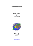
User Manual
Version 1.6
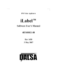
User Documentation for Senozon Via 1.6
© 2011-2015 Senozon AG
2015-10-15
Contents
1
1.1
1.2
1.3
1.4
Getting Started
System Requirements
Installation . . . . . .
License . . . . . . . .
First visualization . . .
.
.
.
.
.
.
.
.
.
.
.
.
.
.
.
.
.
.
.
.
.
.
.
.
.
.
.
.
.
.
.
.
.
.
.
.
.
.
.
.
.
.
.
.
.
.
.
.
.
.
.
.
.
.
.
.
.
.
.
.
.
.
.
.
.
.
.
.
.
.
.
.
.
.
.
.
.
.
.
.
.
.
.
.
.
.
.
.
.
.
.
.
.
.
.
.
.
.
.
.
.
.
.
.
.
.
.
.
.
.
.
.
.
.
.
.
.
.
.
.
.
.
.
.
.
.
.
.
.
.
.
.
.
.
.
.
.
.
.
.
.
.
.
.
.
.
.
.
.
.
.
.
.
.
.
.
.
.
.
.
.
.
.
.
.
.
.
.
1
1
1
1
2
2
2.1
2.2
2.3
2.4
2.5
2.6
Application Overview
Main Window . . . . . .
Toolbar . . . . . . . . . .
Visualization Area . . .
Time and Speed Controls
Control Section . . . . .
Query Section . . . . . .
.
.
.
.
.
.
.
.
.
.
.
.
.
.
.
.
.
.
.
.
.
.
.
.
.
.
.
.
.
.
.
.
.
.
.
.
.
.
.
.
.
.
.
.
.
.
.
.
.
.
.
.
.
.
.
.
.
.
.
.
.
.
.
.
.
.
.
.
.
.
.
.
.
.
.
.
.
.
.
.
.
.
.
.
.
.
.
.
.
.
.
.
.
.
.
.
.
.
.
.
.
.
.
.
.
.
.
.
.
.
.
.
.
.
.
.
.
.
.
.
.
.
.
.
.
.
.
.
.
.
.
.
.
.
.
.
.
.
.
.
.
.
.
.
.
.
.
.
.
.
.
.
.
.
.
.
.
.
.
.
.
.
.
.
.
.
.
.
.
.
.
.
.
.
.
.
.
.
.
.
.
.
.
.
.
.
.
.
.
.
.
.
.
.
.
.
.
.
.
.
.
.
.
.
.
.
.
.
.
.
.
.
.
.
.
.
.
.
.
.
.
.
.
.
.
.
.
.
.
.
.
.
.
.
.
.
.
.
.
.
.
.
.
.
.
.
4
4
5
5
5
6
6
3 Visualizing Data
3.1 Working with Layers . . . . . . . .
3.1.1 Creating Layers . . . . . . .
3.1.2 Create Layers Automatically
3.1.3 Layer Styles . . . . . . . . .
3.2 Layers . . . . . . . . . . . . . . . .
3.2.1 Network . . . . . . . . . . .
3.2.2 Vehicles . . . . . . . . . . . .
3.2.3 Activities . . . . . . . . . . .
3.2.4 Facilities . . . . . . . . . . .
3.2.5 Dynamic Link Attributes . .
3.2.6 Difference Network . . . . .
3.2.7 Link Volume Differences . .
3.2.8 Shape File . . . . . . . . . .
3.2.9 XY-Plotter . . . . . . . . . .
3.2.10Image . . . . . . . . . . . . .
3.3 Views . . . . . . . . . . . . . . . .
3.4 Presets . . . . . . . . . . . . . . .
.
.
.
.
.
.
.
.
.
.
.
.
.
.
.
.
.
.
.
.
.
.
.
.
.
.
.
.
.
.
.
.
.
.
.
.
.
.
.
.
.
.
.
.
.
.
.
.
.
.
.
.
.
.
.
.
.
.
.
.
.
.
.
.
.
.
.
.
.
.
.
.
.
.
.
.
.
.
.
.
.
.
.
.
.
.
.
.
.
.
.
.
.
.
.
.
.
.
.
.
.
.
.
.
.
.
.
.
.
.
.
.
.
.
.
.
.
.
.
.
.
.
.
.
.
.
.
.
.
.
.
.
.
.
.
.
.
.
.
.
.
.
.
.
.
.
.
.
.
.
.
.
.
.
.
.
.
.
.
.
.
.
.
.
.
.
.
.
.
.
.
.
.
.
.
.
.
.
.
.
.
.
.
.
.
.
.
.
.
.
.
.
.
.
.
.
.
.
.
.
.
.
.
.
.
.
.
.
.
.
.
.
.
.
.
.
.
.
.
.
.
.
.
.
.
.
.
.
.
.
.
.
.
.
.
.
.
.
.
.
.
.
.
.
.
.
.
.
.
.
.
.
.
.
.
.
.
.
.
.
.
.
.
.
.
.
.
.
.
.
.
.
.
.
.
.
.
.
.
.
.
.
.
.
.
.
.
.
.
.
.
.
.
.
.
.
.
.
.
.
.
.
.
.
.
.
.
.
.
.
.
.
.
.
.
.
.
.
.
.
.
.
.
.
.
.
.
.
.
.
.
.
.
.
.
.
.
.
.
.
.
.
.
.
.
.
.
.
.
.
.
.
.
.
.
.
.
.
.
.
.
.
.
.
.
.
.
.
.
.
.
.
.
.
.
.
.
.
.
.
.
.
.
.
.
.
.
.
.
.
.
.
.
.
.
.
.
.
.
.
.
.
.
.
.
.
.
.
.
.
.
.
.
.
.
.
.
.
.
.
.
.
.
.
.
.
.
.
.
.
.
.
.
.
.
.
.
.
.
.
.
.
.
.
.
.
.
.
.
.
.
.
.
.
.
.
.
.
.
.
.
.
.
.
.
.
.
.
.
.
.
.
.
.
.
.
.
.
.
.
.
.
.
.
.
.
.
.
.
.
.
.
.
.
.
.
.
.
.
.
.
.
.
.
.
.
.
.
.
.
.
.
.
.
.
.
.
.
.
.
.
.
.
.
.
.
.
.
.
.
.
.
.
.
.
.
.
.
.
.
.
.
.
.
.
.
.
.
.
.
.
.
.
.
.
.
.
.
.
.
.
.
.
.
.
.
.
.
.
.
.
.
.
.
.
.
.
.
.
.
.
.
.
.
.
.
.
.
.
.
.
.
.
.
.
7
7
7
8
8
8
9
9
10
10
11
11
11
12
13
13
14
14
4
4.1
4.2
4.3
4.4
4.5
4.6
4.7
4.8
.
.
.
.
.
.
.
.
.
.
.
.
.
.
.
.
.
.
.
.
.
.
.
.
.
.
.
.
.
.
.
.
.
.
.
.
.
.
.
.
.
.
.
.
.
.
.
.
.
.
.
.
.
.
.
.
.
.
.
.
.
.
.
.
.
.
.
.
.
.
.
.
.
.
.
.
.
.
.
.
.
.
.
.
.
.
.
.
.
.
.
.
.
.
.
.
.
.
.
.
.
.
.
.
.
.
.
.
.
.
.
.
.
.
.
.
.
.
.
.
.
.
.
.
.
.
.
.
.
.
.
.
.
.
.
.
.
.
.
.
.
.
.
.
.
.
.
.
.
.
.
.
.
.
.
.
.
.
.
.
.
.
.
.
.
.
.
.
.
.
.
.
.
.
.
.
.
.
.
.
.
.
.
.
.
.
.
.
.
.
.
.
.
.
.
.
.
.
.
.
.
.
.
.
.
.
.
.
.
.
.
.
.
.
.
.
.
.
.
.
.
.
.
.
.
.
.
.
.
.
.
.
.
.
.
.
.
.
.
.
.
.
.
.
.
.
.
.
.
.
.
.
.
.
.
.
.
.
.
.
.
.
.
.
.
.
.
.
.
.
.
.
.
.
.
.
.
.
.
.
15
16
16
17
17
17
18
18
19
Analyses and Interactive Queries
Show Coordinate . . . . . . . . .
Show Agent Plan . . . . . . . . .
Find Network Element . . . . . .
Link Volumes . . . . . . . . . . .
Intersection Flows . . . . . . . .
Select Link Analysis . . . . . . .
Select Facility Analysis . . . . . .
Facility Charts . . . . . . . . . . .
.
.
.
.
.
.
.
.
i
Contents
5 Public Transport
5.1 Overview . . . . . . . . . . . . . . . . . . . . .
5.2 Layers . . . . . . . . . . . . . . . . . . . . . .
5.2.1 Transit Schedule . . . . . . . . . . . . .
5.2.2 Transit Stats . . . . . . . . . . . . . . .
5.2.3 Passenger Flows . . . . . . . . . . . . .
5.3 Queries . . . . . . . . . . . . . . . . . . . . .
5.3.1 Transit Stop . . . . . . . . . . . . . . .
5.3.2 Transit Line . . . . . . . . . . . . . . . .
5.3.3 Departures . . . . . . . . . . . . . . . .
5.4 Transit Route Analysis . . . . . . . . . . . . .
5.4.1 Passengers Entering/Leaving . . . . .
5.4.2 Vehicle Load, Aggregated Vehicle Load
5.4.3 Route Grid . . . . . . . . . . . . . . . .
5.4.4 Route Flows . . . . . . . . . . . . . . .
.
.
.
.
.
.
.
.
.
.
.
.
.
.
.
.
.
.
.
.
.
.
.
.
.
.
.
.
.
.
.
.
.
.
.
.
.
.
.
.
.
.
.
.
.
.
.
.
.
.
.
.
.
.
.
.
.
.
.
.
.
.
.
.
.
.
.
.
.
.
.
.
.
.
.
.
.
.
.
.
.
.
.
.
.
.
.
.
.
.
.
.
.
.
.
.
.
.
.
.
.
.
.
.
.
.
.
.
.
.
.
.
.
.
.
.
.
.
.
.
.
.
.
.
.
.
.
.
.
.
.
.
.
.
.
.
.
.
.
.
.
.
.
.
.
.
.
.
.
.
.
.
.
.
.
.
.
.
.
.
.
.
.
.
.
.
.
.
.
.
.
.
.
.
.
.
.
.
.
.
.
.
.
.
.
.
.
.
.
.
.
.
.
.
.
.
.
.
.
.
.
.
.
.
.
.
.
.
.
.
.
.
.
.
.
.
.
.
.
.
.
.
.
.
.
.
.
.
.
.
.
.
.
.
.
.
.
.
.
.
.
.
.
.
.
.
.
.
.
.
.
.
.
.
.
.
.
.
.
.
.
.
.
.
.
.
.
.
.
.
.
.
.
.
.
.
.
.
.
.
.
.
.
.
.
.
.
.
.
.
.
.
.
.
.
.
.
.
.
.
.
.
.
.
.
.
.
.
.
.
.
.
.
.
.
.
.
.
.
.
.
.
.
.
.
.
.
.
.
.
.
.
.
.
.
.
.
.
.
.
.
.
.
.
.
.
.
.
.
.
.
.
.
.
.
.
.
.
.
.
.
.
.
.
.
.
.
.
.
.
.
.
.
.
.
.
.
.
.
.
.
.
.
.
.
.
.
.
.
.
.
.
.
.
.
.
.
.
.
.
.
.
.
.
.
.
21
21
21
21
22
22
22
23
23
23
23
23
23
24
24
6 Map Background
6.1 Overview . . . . .
6.2 Layers . . . . . .
6.2.1 GeoTIFF . .
6.2.2 WebMap .
.
.
.
.
.
.
.
.
.
.
.
.
.
.
.
.
.
.
.
.
.
.
.
.
.
.
.
.
.
.
.
.
.
.
.
.
.
.
.
.
.
.
.
.
.
.
.
.
.
.
.
.
.
.
.
.
.
.
.
.
.
.
.
.
.
.
.
.
.
.
.
.
.
.
.
.
.
.
.
.
.
.
.
.
.
.
.
.
.
.
.
.
.
.
.
.
.
.
.
.
.
.
.
.
.
.
.
.
.
.
.
.
.
.
.
.
26
26
26
26
26
7 Car Counts
7.1 Car Counts Layer . . . . . . . . . . . . . . . . . . . . . . . . . . . . . . . . . . . . . . . . . . . . .
27
27
8
8.1
8.2
8.3
29
29
29
30
.
.
.
.
.
.
.
.
.
.
.
.
.
.
.
.
.
.
.
.
.
.
.
.
.
.
.
.
.
.
.
.
.
.
.
.
.
.
.
.
.
.
.
.
.
.
.
.
.
.
.
.
.
.
.
.
.
.
.
.
.
.
.
.
Aggregator
Overview . . . . . . . . . . . . . . . . . . . . . . . . . . . . . . . . . . . . . . . . . . . . . . . . . .
Aggregating Point Data . . . . . . . . . . . . . . . . . . . . . . . . . . . . . . . . . . . . . . . . .
Aggregating OD Data . . . . . . . . . . . . . . . . . . . . . . . . . . . . . . . . . . . . . . . . . . .
9 Recording Movies
9.1 Overview . . . . . . . . . . . . . . . .
9.2 Creating Movies . . . . . . . . . . . .
9.2.1 Recording a Movie . . . . . . .
9.2.2 Movie Settings . . . . . . . . .
9.2.3 Converting Images to a Movie
9.3 Movie Formats . . . . . . . . . . . .
.
.
.
.
.
.
32
32
32
32
33
33
34
10 Scripting Via
10.1 Overview . . . . . . . . . . . . . . . . . . . . . . . . . . . . . . . . . . . . . . . . . . . . . . . . . .
10.1.1Script Editor . . . . . . . . . . . . . . . . . . . . . . . . . . . . . . . . . . . . . . . . . . . .
35
35
35
11 Common Steps
11.1 Optimizing Events loading . . . . . . . . . . . . . . . . . . . . . .
11.2 Color some vehicles differently . . . . . . . . . . . . . . . . . . .
11.3 Distribute activity locations to actual coordinates . . . . . . . . .
11.4 Customizing the list of available Coordinate Reference Systems .
37
37
37
38
39
.
.
.
.
.
.
.
.
.
.
.
.
.
.
.
.
.
.
.
.
.
.
.
.
.
.
.
.
.
.
.
.
.
.
.
.
.
.
.
.
.
.
.
.
.
.
.
.
.
.
.
.
.
.
.
.
.
.
.
.
.
.
.
.
.
.
.
.
.
.
.
.
.
.
.
.
.
.
.
.
.
.
.
.
.
.
.
.
.
.
.
.
.
.
.
.
.
.
.
.
.
.
.
.
.
.
.
.
.
.
.
.
.
.
.
.
.
.
.
.
.
.
.
.
.
.
.
.
.
.
.
.
.
.
.
.
.
.
.
.
.
.
.
.
.
.
.
.
.
.
.
.
.
.
.
.
.
.
.
.
.
.
.
.
.
.
.
.
.
.
.
.
.
.
.
.
.
.
.
.
.
.
.
.
.
.
.
.
.
.
.
.
.
.
.
.
.
.
.
.
.
.
.
.
.
.
.
.
.
.
.
.
.
.
.
.
.
.
.
.
.
.
.
.
.
.
.
.
.
.
.
.
.
.
.
.
.
.
.
.
.
.
.
.
.
.
.
.
.
.
.
.
.
.
.
.
.
.
.
.
.
.
.
.
.
.
.
.
.
.
Appendices
40
A
A.1
A.2
A.3
Configuration
Change the RAM-Limit . . . . . . . . . . . . . . . . . . . . . . . . . . . . . . . . . . . . . . . . . .
Switch between 32-bit and 64-bit versions . . . . . . . . . . . . . . . . . . . . . . . . . . . . . .
Setting Colors based on Attribute Values . . . . . . . . . . . . . . . . . . . . . . . . . . . . . . . .
41
41
41
42
B
What's new in Via 1.6?
43
ii
1
Getting Started
1.1
System Requirements
Operating System:
Windows: Senozon Via runs on Windows XP SP 3 or newer, including Windows 7 and Windows 8.
Linux: Senozon Via requires an existing installation of Java 7 or newer. Oracle’s Java Runtime Environment
(JRE) is recommended, which can be downloaded from http://java.oracle.com/. Please note that
OpenJDK and GCJ are sadly known to cause problems when running Via on Linux.
Mac OS X: Senozon Via runs on Mac OS X 10.7.3 (Lion) or later.
Memory:
To run Senozon Via, make sure you have enough RAM. Small scenarios can usually be visualized with less
than 1 GB of RAM. Typical scenarios with around 1 million agents can be run with around 3 GB of RAM.
1.2
Installation
The application does not require any special installation. You can just unzip the downloaded file and move
the directory to whatever place you like (e.g. Program Files on Windows, or /Applications/ on Mac OS X).
In the Linux distribution, a starter shell script is provided which can be used as the target of a symlink
or for a custom launcher.
1.3
License
To run Senozon Via, you need a license file. When you start Via for the first time, the application will ask
you for the license file, in order to fully setup and start the application. You can manage your license later
at any point by selecting the menu entry Help > License Manager….
1
Chapter 1. Getting Started
1.4
First visualization
This section gives just a quick overview how to do some basic visualization with the sample data provided.
See the following chapters for more details and a more extensive description of available functionality.
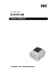
Start Via, and after the main window appears, choose File > Add Data…. Navigate to the sample data and
select the file network.xml. Choose File > Add Layer… and click on Network. The just previously loaded file is
suggested to be used, which is okay. Click on Add to add the network layer. The network should be shown
in the visualization area and the network layer be listed next to it.
Figure 1.1: The main window, with the network layer added
Now let’s add some vehicles to it. Again, choose File > Add Data… and select the file 10.events.xml.gz.
Then, add a Vehicles Layer (File > Add Layer…, select Agents > Vehicles, click Add). The vehicles layer will also
be listed on the side of the visualization area. As event files can be rather large, they are not automatically
parsed. Instead, layers that depend on events, show a button Load Data which must be clicked manually
in order to parse the data from the events. Click this button to start the parsing of the events. Once this
process is finished, a timeline appears beneath the visualization area. Move the slider to some point in time
(e.g. to 8 o’clock) or move the speed slider next to it to animate the shown time. Soon you should see green
triangles, representing vehicles, move around the network.
Play around with the Size and Offset sliders in the layers’ settings area, and see which effect they have
on the visualization. Fig. 1.2 gives you an impression how the visualization could look like after modifying
those settings.
2
1.4 First visualization
Figure 1.2: Network and Vehicles loaded and visualized
3
2
Application Overview
2.1
Main Window
Figure 2.1: The main window
The main application window can be differentiated into the following areas:
Toolbar at the top of the window.
Visualization Area taking up most of the place, in the middle of the window.
Time and Speed Controls below the visualization area.
Control Section to manage the visualized data on the left side of the window.
Query Section on the right side to work with interactive queries.
All the parts can be freely re-arranged by drag and drop on the title bars of the parts. In case you want
to restore the default arrangement of the components, select menu Window > Reset Window State. In the
following, the main functionality of the different components will be described in more details.
4
2.2 Toolbar
2.2
Toolbar
Figure 2.2: The Toolbar
The actual buttons on the toolbar depend on the available plugins. The buttons shown in Fig. 2.2 are standard buttons and available in all installations:
Save Save the currently loaded data to a file. This stores all data required for displaying the loaded layers
in a file, together with the current display configuration (colors, sizes, etc). The filename of such files
ends on “.via”. Note: Storing big data sets can take several minutes.
Open Loads the data from a previously saved file. Any already loaded layers will be removed.
Mouse for Moving If active, the mouse pointer can be used to move the visualized region.
Agent Plan Query Activates the agent plan query (see Sec. 4.2).
Zoom In, Zoom Out, Zoom to Full Extent Zooming functionality
PDF-Export Takes a single PDF-Snapshot of the display area. Note: Taking a PDF-snapshot can take some
time on complex visualizations with many agents being shown.
Screenshot-Recording If activated, constantly saves screenshots of the visualization area. The location
where the screenshots are saved can be configured in the application’s options.
Single Screenshot Saves the current display as a bitmap image.
2.3
Visualization Area
The visualization area covers the biggest part of the main window. Here, your network, vehicles and other
data will be visualized. Which data is visualized is controlled by the Layers Control (see Sec. 2.5). You can
navigate in the visualization area by clicking and dragging the area with your mouse while the corresponding
functionality is activated in the toolbar. When some other query tool is activated, use the middle mouse
button to drag the visualization area, or switch back to the regular mouse functionality by clicking on in
the toolbar. To zoom in or out, you can either use the corresponding buttons in the toolbar, or use the scroll
wheel on your mouse.
2.4
Time and Speed Controls
Below the visualization area, you find two sliders: The first controls the current time shown, while the
second controls how quick the time advances in the visualization.
Directly after starting Via, the time slider does not show any indication of time. Only after loading some
time-dependent data and visualizing it by adding corresponding layers will the slider display the range of
time for which data is available. You can customize the shown range of time by using the Menu Time >
Set Custom Time Range…. The Time menu also offers several commands to control which point in time is
visualized.
5
Chapter 2. Application Overview
2.5
Control Section
Figure 2.3: Control Switches
In the control sections, various settings for controlling the visual appearance or the available data are presented. The controls are organized into four groups, which can be switched by clicking on the different
icons:
Data Sources Add data files (e.g. network.xml, events.xml.gz, zones.shp) to the application to make them
available for visualization. Either click on the green plus-button at the bottom of the area, or just drag
and drop files into the area to add them.
Layers Add and manage “layers”, visual representations of loaded data. Each layer is typically responsible
for displaying one aspect of the data (e.g. the network, vehicles, activities, one shape file).
Agent / ID Groups Manage sets of agent ids, which can be used by layers to customize the visualization.
For an example, see Sec. 11.2.
Overlays Manage the appearance of overlays over the visualization area, like the clock shown in the topright corner.
2.6
Query Section
One of Via’s strength is its wide range of analyses it offers. Most of the analyses start by querying one of
the visualized objects, e.g. a vehicle, a transit stop, a facility. Based on such a selection, additional queries
are possible, e.g. the lines serving a transit stop, the number of persons in a facility. All these queries and
their results are available in the query section. Chpt. 4 looks at the available queries in more detail. In
addition, the chapters about the different plugins (e.g. Chpt. 5 for the Public Transport plugin) also refer to
the queries provided by the respective plugin.
6
3
Visualizing Data
Data visualized in Via is organized by layers. Each layer is responsible for visualizing one data set. Thus, Via
provides layers for visalizing networks, facilities, agents’ activities and trips, public transport stops, or just
generic points in space.
3.1
3.1.1
Working with Layers
Creating Layers
To create a new layer, make sure that the needed data is available and loaded into the application. Then,
switch to the Layers Control and click the green plus-button at the bottom of the panel, or choose File > Add
Layer…
from
the
menu.
Figure 3.1: Creating a new layer for visualizing data
Once a layer is created, it will appear in the list of layers, along with settings
offered by the layer. Layers can by hidden by unticking the checkbox in
front of the layer name. The order of the layers can be changed by clicking
in the area next to the layer name and dragging the layer up or down in
the list of all layers.
On the right end of the layer’s title bar, a triangle icon offers additional
options to work with a layer in a popup. By default, options to rename or
remove a layer are available. Certain layers provide additional functionality
in this place as well, such as the network layer depicted.
Figure 3.2: A layer with settings, and the layer options
7
opened.
Chapter 3. Visualizing Data
3.1.2
Create Layers Automatically
The typical process to visualize some data consists of at least two steps:
Add the necessary data file, then create a layer using this data to show
something. This can be simplified by instructing Via to automatically create certain layers when specific kinds of data is loaded.
Switch to the Data Sources control (first button in the control section). At the bottom, you’ll see a little
gear icon. Click on it and select Automatically Create Layers…. A dialog will open where you can select which
layers should be automatically created.
Figure 3.3: Automatically create new layers when adding data
Please note that when you are adding multiple data files of the same type (e.g. multiple networks and
multiple event files), Via might not create certain layers due to the ambiguity of which files to combine (e.g.
which network and which events to create a Vehicles layer).
3.1.3
Layer Styles
Most layers include options to change the visual appearance of the shown data. This is great as depending
on the zoom level, different settings might be helpful: Looking at a small detail of a road network, it might
be desireable to have the links shown with a heavy stroke and some offset, but looking at the full network, a
thin stroke and no offset often looks better. If you often change between two or more zoom levels, keeping
track of all the right settings is very cumbersome. Styles help to store the state of the visualization options,
so it is easy to switch between two or more visual setups with ease. Styles are saved in *.via files, so they
can also be used to define presets to be used during a presentation, e.g. along with Views (see Sec. 3.3).
To access the styles option of a layer, open its option menu. If the layer
supports styles, you’ll see the entries Save Style…, Use Style, Manage Styles…,
Set As Default Style…. To save the current visualization options of this
layer as a style, just select Save Style… and enter a name. The style will then
appear in the sub-menu of Use Style, where it can be selected. If you have
a corporate appearance, or prefer other defaults than Via’s developers, you
can define your own default style for this layer by selecting Set As Default
Style. Then, all new layers of this type will use your current settings.
With Manage Styles… you can delete styles, restore the application default style, and define styles as being global. By default, styles are related Figure 3.4: Access to the
to the current visualization, and are stored in *.via files. But if you want styles for a layer.
some styles available all the time, no matter what data you are visualizing, you can define those styles as global using the Manage Styles… dialog.
A global style is stored locally with the applications options, so every time you start Via on this machine, the
style will be available under Use Style.
3.2
Layers
In the following sections, the layers available by a default installation of Via are described. Plugins can add
additional layers, which are described in their own sections.
8
3.2 Layers
3.2.1
Network
Displays a network.
Requires a loaded network file.
Using the settings, it is possible to offset links either to the
left or the right such that the links in opposing directions
are not drawn on top of each other.
The colors and width of links can be modified by clicking on the gearwheel (options) icon. It is possible to assign
different colors to links with different allowed modes, different number of lanes, different capcacity and other attributes. Also, one can display links with different width
depending on links’ attributes (allowed modes, number of
lanes, and others). When setting the values based on allowed modes and a link should match multiple modes,
separate the various modes with a comma. If a link Figure 3.5: Setting the colors and width of links
should match having at least one specific mode, enclose in a network
the mode with asterisks (“*”). The color of a link is determined by the first (top-most) mode-description that
matches the links’ transport modes.
The list of attributes available to set the appearance of links in the network can be extended with additional attributes loaded from a variaty of files. Supported files are MATSim’s Object Attributes saved as
XML file, tab-separated text files, or CSV files. To load additional attributes, click on the small triangle in the
layer settings (see Fig. 3.2) and select Attributes Manager….
3.2.2
Vehicles
Displays vehicles at their current position in the network.
Requires a loaded network file and an events or population file.
The vehicles layer displays the position of vehicles in the
network. The vehicles can be colored based on a number
of attributes, including absolute or relative speed (relative
to the links’ free speed). To change the display style of vehicles, click on the color wheel icon. A dialog as in Fig. 3.6
will show where the color and the style of the vehicles can
be set. It is even possible to have different styles for different groups of vehicles. Sec. 11.2 explains in detail how
this can be done.
If you have the FancyVehicles plugin, you can define
your own display styles given the options available in the
FancyVehicles’ settings available in the Tools menu.
Figure 3.6: Setting the styles for vehicles
Other layers (e.g. TransitStats) or data sources can
provide additional attributes that can be used to color
agents, for example the number of passengers, or agent-attributes from a population file.
9
Chapter 3. Visualizing Data
3.2.3
Activities
Displays the locations where agents are currently performing an activity.
Requires a loaded network file and an events or population file.
The activity layer displays a colored dot at each location where an agent is currently located, performing an
activity. Different types of activities can be visualized with different colors. To create an activity layer, you
have two possibilities:
• Load the activity data from events. The location (based on link ids) and the start and end time of
activities are retrieved from events.
• Load the activity data from population. The location (link id or, if given, the exact coordinate) as well
as the start and end time of activities are extracted from a plans file.
Only one of the two sources (events, or population) can be used to create an activities layer. If you want the actual activity times from events,
but want to use the exact location as given in a plans file, follow the steps
outline in Sec. 11.3.
Each activity type can be shown in a different color. To setup the colors,
click on the color wheel icon. Then, assign colors to the different activity
types. To add a new activity type, click the “+” icon. Note that you can
use an asterisk as wildcard character to match multiple, similar activity
types and assign them one common color. To learn what activity types
actually occur in the data, click on the little gearwheel icon and select Find
attributs…. A list of all activity types found in the loaded data will be shown,
along with the color in which they would currenctly be displayed.
Please note that the Activities Layer may slow down the visualization
enormously if a large number of agents is shown.
3.2.4
Figure 3.7: Setting the colors
for different activity types
Facilities
Displays the locations of facilities.
Requires a loaded facilities file.
Figure 3.8: Home facilities displayed over a planning network
Facilities are an optional dataset in MATSim, which are often used to model location choice or are also used
during the initial demand modeling. Displayed facilities can be filtered by activity type, so only facilities
that offer a specific activity type are shown. In addition, facilities can be displayed only when the facility is
10
3.2 Layers
opened, according to the opening times defined in facilities. If the facilities are filtered, the opening time of
the filtered activity type is used, otherwise a facility is displayed if at least one of its activity options is open.
3.2.5
Dynamic Link Attributes
Displays traffic volumes or average link speeds by coloring the links in the network.
Requires a loaded network file and an events file.
This layer calculates two time-dynamic values for each link: (a) traffic volume (number of vehicles passing
a link), (b) average speed on a linkk. This information is then provided as additional attributes to the Network, such that link volumes and link speeds can be selected as an attribute to display the network. Both
attributes can be aggregated to different time windows, link volumes provided to the network are always
scaled to hourly values. This has the advantage that the assigned color ramp does not have to be adapted
if the aggregation level is changed.
Absolute and relative link volumes are provided:
Absolute link volumes are the actual number of vehicles counted per link.
Relative link volumes are values between 0.0 and 1.0 corresponding to the amount of vehicles compared
to the available capacity of the link.
Note: This layer was originally called “Link Volumes”
3.2.6
Difference Network
Displays the absolute or relative difference between two link attributes (from the same or different networks).
Requires one or two loaded networks.
This layer allows to calculate the absolute or relative difference of two attributes. The attributes can be from
the same or from two different networks, and the attributes can be scaled, e.g. to compare link volumes
between two different sample scenarios.
3.2.7
Link Volume Differences
Displays absolute or relative difference between two link volume data sets.
Requires a loaded network file and two events files.
Note: This layer is the predecessor of the Difference Network Layer and will be remove in a later version.
This layer calculates the difference of two link volume data
sets, useful to show differences in two scenarios. This
allows you to load two Link Volume layers based on two
different events files, one e.g. being a base case and the
second one a case study. The calculated difference is provided as additional attribute to the Network. To display
the link volume differences, one has thus to select the corresponding attribute in the Network display settings.
The difference can be computed in three different
ways, one named “absolute difference”, and two variants
for the “relative difference”. Make sure to select your preferred variant for the relative difference in the layer settings.
Figure 3.9: Selecting the right attribute for displaying a network
The meaning of the three alternatives are:
Absolute: the difference between the absolute link volumes of the two cases.
11
Chapter 3. Visualizing Data
Relative: Relative diff. of B to A : The difference between the two link volumes per link is set in relation to
the link volume of the first one.
Relative: abs. diff. of rel. volumes : The absolute difference between the two relative link volumes.
To clarify the matter, consider the following example: A link in the network has a defined capacity of 2000
veh/h. In the base case, 1500 veh/h were counted. In the study case, 1000 veh/h are counted.
• The absolute difference would be calculated as 1000 – 1500, resulting in an absolute difference of
–500 veh/h.
• The first relative difference is calculated as (1000 – 1500) / 1500, resulting in –0.33. This can be interpreted as having 33% less traffic in the study case than in the base case.
• The second relative difference is calculated as (1000 / 2000) - (1500 / 2000), resulting in –0.25, or 25%
less capacity of the link used.
3.2.8
Shape File
Displays arbitrary shape files, e.g. for background maps.
Requires a loaded shape file.
Figure 3.10: Options for Shape
Files
This layer allows one to visualize shape files (points, line and areas are
supported). First, load a shape file as data source, then create a layer for
it. If the shape file is shown in the wrong place, or even rotated, change
the options in the data sources view. First, make sure the shape file is
in the correct coordinate reference system (CRS). Next, if the shape file
appears to be rotated and squeezed, select the checkbox “Use Long/Lat
instead of Lat/Long”. This is due the fact that shape files (or more exactly:
coordinate systems) do not specify if the first coordinate is the longitude
or the latitude. The list of available coordinate reference systems can be
adapted in Via’s options (menu File > Options… on Windows and Linux, Via
> Preferences… on Mac OS X).
In the layer’s option menu (the triangle on the right side of the layer’s
title), Shape layers offer the option to display a shape file only during a
specific time window. This can be used e.g. to highlight areas in a timedependent manner.
Figure 3.11: Two Shape file layers added for visualizing nature and railroad tracks
12
3.2 Layers
3.2.9
XY-Plotter
Displays colored dots at coordinates specified in a file
Requires a file containing coordinates and attributes (see below)
The XY-Plotter plots dots at specific locations given in a file. This layer is mostly useful to quickly test some
data before or after conversion from other formats. Just dump some coordinate values into a file and have
a look if their distribution makes visually sense and is what you expected.
A variety of file formats are supported:
.xy, .txt Text files ending on .xy were traditionally the only format supported by Via. By now, the files can
also end on .txt. Such files must contain at least two columns of data, separated with a tab. The first
column contains usually the x-coordinate, while the second contains the y-coordinate. Attributes can
be included in additional columns.
.csv CSV (Comma separated values) files can often be created by spreadsheet applications. Each attribute,
including x- and y-coordinates, should be stored in a separate column. Via[] supports CSV files which
use comma or semicolon as field separator.
.gpx GPS devices often record points in GPX files. Via can load GPX files and extract the coordinates from
recorded tracks and waypoints.
In the full version of Via, the layer offers a lot more functionality and supports additional attributes for
each data point. When adding an xy data source, a dialog containing import options can be shown by clicking
the corresponding button in the data sources view. In the dialog, attributes can be selected that should be
imported, the name and data type can be specified for each attribute, and it can be specified with columns
contain the X and Y values.
Figure 3.12: Settings for importing XY data
The layer settings offer a lot of functionality to work with the additional attributes. For example, it
is possible to color the points based on an attribute’s value, or change the symbol or the size of the dot
according to an attribute’s value. In addition, points can be displayed only during a specific time window,
also based on attributes. If some of the points form a logical group, e.g. points from a GPS track of a single
person, and group membership is available in an attribute, it is even possible to interpolate the location of
time-dependent points along the time of day.
3.2.10
Image
Displays arbitrary images at custom defined locations
Requires a loaded image file
This layer allows to display custom images at fixed locations on the screen. It can be used to show custom
backgrounds images or logos.
13
Chapter 3. Visualizing Data
Figure 3.13: Settings for displaying XY data
3.3
Views
Do you prepare for a presentation or a movie recording, or need to make multiple screenshots of the same
region? It happens very fast that one moves the viewport around in Via, or one zooms in or out to have
a quick look at some other region. But how to get back to that fixed region you wanted to have the same
screenshots?
Views store the the currently viewed extent of your scenario. So you can define multiple views, e.g. one
for a birds-eye perspective, one for a specific intersection, and another one for a certain corridor. It is then
easy to switch between the different extents by just a few mouse clicks, or animate the transition from the
current view point to another.
To define a view select menu Views > Save Current View….
To change to saved view select menu Views > Jump to > View.
To incrementally move to a view select menu Views > Fly to > View.
To delete a view select menu Views > Manage Views….
In the Views Manager, it is also possible to specify options how fast the “Fly to” operation works.
3.4
Presets
Presets allow you to restore the visibility and styles of multiple layers at once. Optionally, Presets also
support switching to a specific View and time, as well as changing the animation speed. This allows Presets
to be used to quickly demonstrate several aspects of a scenario, e.g. zooming in to an intersection showing
single vehicles driving slowly past the node, or switching to a view showing a larger region and only transit
vehicles during the evening rush hour.
Presets can be created and selected using the menu at the bottom of the Layer list.
14
4
Analyses and Interactive Queries
Many layers provide some functionality to query and analyze the loaded and visualized data. The results
of such queries are typically displayed in the query section right to the visualization area. There, additional
options are often available, depending on the active query.
Queries can be issued in multiple ways:
• By activating the query (clicking on the query-button) and then clicking in the visualization area, e.g.
clicking on a link or a vehicle. Query-Buttons typically look like .
• By activating the query (clicking on the query-button) and then entering an argument, e.g. the link or
agent id, into a search field in the query controls part.
• By following one of the query option in a query result. For this, click on the little triangles shown next
to query results: .
• By a right-click in the visualization area to follow up on an existing query result.
Figure 4.1: Activation of the network query and a sample query result.
Fig. 4.1 shows the several ways queries can be started:
1.
2.
3.
4.
By activating the query tool and clicking on a link.
By activating the query tool and enter the link id.
By clicking on a query result button and selecting a follow-up query.
By right-clicking in the visualization area and selecting a follow-up query.
15
Chapter 4. Analyses and Interactive Queries
In the following, the queries provided by the layers available in the standard version of Via are presented.
Plugins may provide additional layers with queries.
4.1
Show Coordinate
This query is quite simple: It allows you to enter a coordinate’s x and y values and display the coordinate’s
location in the visualization area. This is useful if you want to highlight a specific location, e.g. for screenshots, but don’t want to create and load a coordinates files (see Sec. 3.2.9) for this. Make sure to have the
“Move View” activated in the toolbar and switch to the Queries Control, where you can enter the x and y
values of the coordinate.
Figure 4.2: Locate a specific coordinate
4.2
Show Agent Plan
Requires at least one of Vehicles Layer, Activities Layer
If this query is selected, one can either click on an agent or enter the agent’s id and press Enter to show
an agents day play. Depending on what layers are loaded, the agent’s activities and/or the agent’s legs are
highlighted in the visualization area and listed as a query result. In the query result section, single legs or
activities can be shown or hidden, to customize the presentation of the agent’s (realized) day plan.
Figure 4.3: The complete day plan of one agent visualized
16
4.3 Find Network Element
4.3
Find Network Element
Requires Network Layer
This query can be used to identify links or nodes in a network. It supports a direct search as well as a
reverse search approach: Either you want to know where a specific link or node is located, then you enter
the object’s id into the search field. Or you want to know which link or node it is you see on the viewing
area, then you can just click on the link or node in the viewer. To activate the query, click on the query icon
( ) provided in the network layer settings.
Once a link or node is selected, a number of additional queries are available upon right-clicking into the
visualization area. Examples of such further queries are Link Volumes and Intersection Flows as presented
in the next sections.
4.4
Link Volumes
The Link Volumes query shows the detailed link volumes of the selected link. It allows to aggregate the volumes into different time bins and settings a scaling factor to represent correct volumes if only a population
sample was simulated.
Figure 4.4: Time-dependent volumes on a selected link
4.5
Intersection Flows
The Intersection Flows query shows the number of vehicles that cross the selected node, showing the
different routes the vehicles take. The query supports filtering by time, such that only the flows of a specific
time frame or rush hour can be analyzed. When moving the mouse pointer over one of the flows, the
volumes of only that flow will be shown on the histogram.
The lines’ thickness is typically scaled such that the highest shown volume has a fixed width. This may
lead to interpretation difficulties when comparing two times frames, one with a large number of vehicles
crossing the node and one with a small number of vehicles crossing the node, as both might look similar. To
overcome this problem, it is possible to specify a custom value as largest volume to be used for determining
the scale factor of the lines.
17
Chapter 4. Analyses and Interactive Queries
The chart can be exported into the usual formats (PNG, PDF), but also as animated GIF. In this case, a
GIF image showing the flows hour by hour is created.
Figure 4.5: Time-dependent Intersection Flows
4.6
Select Link Analysis
Requires Network Layer and Vehicles Layer
Selecting one link for this query, it analyzes which vehicles are currently located on that link, and then
highlights all links where those vehicles will travel along during their current trip or even during the whole
day. Instead of all vehicles currently located on the link, the analysis period can be extended to incude all
vehicles on that link in the current quarter, half or full hour or even on the whole day. The query result is
dynamic: If the time changes and vehicles enter or leave the selected link, the highlighted links will change
accordingly depending on the actual vehicles being on the link.
To create a Select Link Analysis, select the corresponding query tool in the network layer’s settings panel
and click a link. Alternatively, you can first select a link with the regular network query (see Sec. 4.3 above),
and then right-click and select “Select Link Analysis”.
4.7
Select Facility Analysis
Requires Facilities Layer, Activities Layer, Vehicles Layer
The Select Facility Analysis is similar to the Select Link Analysis: it shows the routes of vehicles going or
coming from a selected facility. The Select Facility Analysis is available from the settings panel of the layer.
After clicking on a facility, the routes of arriving agents, departing agents, or both, can be visualized.
Agents staying at the facility within the selected time frame can be put into an agent group. This allows
to visualize then only those vehicles, or otherwise filter on those group.
18
4.8 Facility Charts
Figure 4.6: All links travelled by agents currently located in the link in the middle are highlighted
Figure 4.7: The highlighted links change as vehicles enter or leave the selected link
4.8
Facility Charts
Requires Facilities Layer, Activities Layer
If your MATSim scenario uses facilities, it is possible to analyze the number of agents arriving, departing, or
being at a facility. For this, use the facility query and click on a facility. Next, right-click and select Facility
Charts…. A new window will open as shown in Fig. 4.8 which allows you to select the different analyses and
modify the charts.
19
Chapter 4. Analyses and Interactive Queries
Figure 4.8: Facility Load, one of the available Facility Charts
20
5
Public Transport
The functionality described in this chapter is provided by the Public Transport plugin.
5.1
Overview
The public transport plugin provides many functionality for working with transit related data in MATSim.
Most of the functionality is for working with MATSim’s transit schedule data and the outcome from a simulation including public transport.
5.2
5.2.1
Layers
Transit Schedule
Displays transit stop facilities and transit lines.
Requires a loaded transit schedule file.
This layer displays all stop facility locations and supports many of the transit related queries with schedule
data.
Figure 5.1: Locations of transit stop facilities and the route of a single transit line visualized.
21
Chapter 5. Public Transport
5.2.2
Transit Stats
Displays number of persons waiting at transit stop facilities.
Requires a loaded transit schedule, transit vehicles, and events.
Provides data for a number of transit related queries.
The Transit Stats layers is similar to the Transit Schedule layer, but uses Events to extract simulated performance measures instead of the fixed schedule. Thus, it also displays the stop facilities, but can color
them according to the number of passengers waiting at the stops. In addition, it provides data to a lot of
transit-related queries.
5.2.3
Passenger Flows
Displays number of persons entering or leaving a vehicle at a stop.
Requires a loaded transit schedule and events.
The Passenger Flows layer allows to visualize the number of passengers that enter or leave a transit vehicle
at a stop location, including people who change transit lines at a stop. The layer requires the information to
be extracted from the simulation events. The values can be calculated either for all passengers at a stop,
or only concerning a subset of agents specified by an Agent Group (see 11.2). The values are currently only
available for the complete time frame covered by the events, but are not disaggregated into hourly values.
Once the events are loaded, the user can choose from
4 different settings: One can either visualize the number
of passengers entering (boarding) a transit vehicle, or the
number of passengers leaving (alighting) a transit vehicle. For both entering and leaving, either an absolute or
relative value can be visualized. If an absolute option is
chosen, the visualization scales with the absolute number
of passengers boarding or alighting at the stops. Larger
circles then represent more passengers. The relative options are only useful if the events were restricted to a person group during loading. Is this the case and a relative
option is chosen, the visualization scales relative to the
amount of the number of entering or leaving passengers
in the person group compared to all passengers at that
stop. If no person group was specified when loading the
data, the relative values are all set to 100%, resulting in all
drawn circles having the same size.
To clarify the settings, consider the following example: In your region, you have a few stops which are
close to schools, universities or other educational institutes. If you just compare the absolute values without
restriction to a person group, you can visually recognize which stops have the largest amount of passenger
traffic. If you restrict the analysis to a person group, e.g. people aged between 15 and 20, you can recognize
which stops have the highest number of student passengers. If you have restricted the analysis to the
student person group and visualize the values with a relative option, you can recognize at what stop you
have a high share of students. Consider you want to perform a passenger survey specific to students: It
might be easier to find participants at a stop with a high share of student passengers, but not necessarily
at a stop with a high absolute number of students, as at such a stop there could be even more non-student
passengers, making most of the passengers irrelevant for the survey.
Tip: If the user is interested in the amount of passengers per station during a certain time of day only
(e.g. only morning or evening rush hour), this can be achieved by setting a time limitation at the events
data set settings. It is possible to first load the events, set to only the morning rush hour, and afterwards
generate a second Passenger Flows layer and load only the events for the evening rush hour. Use the
possibility to give distinctive names to your layers so you can remember which layer contains which data.
5.3
Queries
There exist several transit related queries, which are to some part dependent on each other. Starting point
for most queries is the default transit query which can be activated by pressing the query button on a transit
22
5.4 Transit Route Analysis
schedule’s settings panel ( ). Once this is active, transit stops can be clicked on in the visualization area,
or transit lines can be looked up in the Query Control section.
5.3.1
Transit Stop
This query allows to identify stop facilities by clicking on them, or by searching for them given their id. If a
transit stats layer is loaded, the query also offers statistics about the number of persons waiting at a stop
location over the time of day in a chart.
5.3.2
Transit Line
This query allows one to highlight the routes of single transit lines (see Fig. 5.1 for an example). For each
transit route, a number of statistics is available if a Transit Stats layer is loaded. For example, it offers a
time-distance diagram to compare the scheduled travel times and the simulated travel times from stop to
stop. It is also possible to show the number of passangers entering and leaving a transit vehicle for each
departure of a route.
A transit line can be queried in different ways:
• The query can be activated using the button on the Transit layer settings panel, then switching to the
Queries Control panel and choose a transit line from the popup menu.
• One can select a link using the network query (see Sec. 4.3) and then select an option on the query
result to list all transit lines serving the selected link.
• One can select a stop, and give list all transit lines serving the selected stop.
Once a transit line and route is selected, clicking on the chart-button opens a new window with different
available analyses for the selected transit route. Sec. 5.4 explains the available transit route analyses in
detail.
5.3.3
Departures
Given a selected stop, one can list the next few departures at that stop, based on the current time. Alternative, having a list of transit lines serving a stop or a link, one can list the departures of specific transit routes
from the list of transit lines.
5.4
Transit Route Analysis
The transit route analyses are available for each transit route. Both a TransitSchedule layer and a TransitStats layer must be loaded for the analyses to work. Some analyses also requre the Vehicles layer to
be loaded. Each analysis can either be applied to exactly one departure of the selected route, of for all departures within a specific time window. If not stated otherwise, the departure time at the first stop of the
route determines if a departure falls within a time window or not.
5.4.1
Passengers Entering/Leaving
This analysis shows the number of passengers entering or leaving at each stop. It also shows the number
of passengers that are within a transit vehicle when it departs at a stop. If multiple departures are selected,
values are accumulated.
5.4.2
Vehicle Load, Aggregated Vehicle Load
The Vehicle Load analysis shows for each departure the number of passengers in a transit vehicle when it
departs at a stop. If multiple departures are selected, values are not aggregated, but shown for each single
departure.
In contrast, the Aggregated Vehicle Load analysis extracts aggregated statistical values from multiple
departures.
23
Chapter 5. Public Transport
Figure 5.2: Vehicle Load per Departure, Aggregated Vehicle Load.
Figure 5.3: Route Grid.
5.4.3
Route Grid
The Route Grid analysis shows for each served transit stop and hour the number of passengers entering or
leaving a transit vehicle of the selected transit line.
5.4.4
Route Flows
This analysis shows the flows of passengers along the transit route: It shows which parts of the route
passengers travel. This analysis gives an easy overview if demand is about equally distributed along a
route, if there are some hubs along the route (e.g. for feeder lines, where most people enter or leave at one
specific stop), or even if a long transit route could be split into two parts without having too many people
needing to switch from one line to another.
24
5.4 Transit Route Analysis
Figure 5.4: Route Flows.
25
6
Map Background
The functionality described in this chapter is provided by the Map Background plugin.
6.1
Overview
The Map Backgorund plugin provides several possibilities to display maps as background images.
6.2
6.2.1
Layers
GeoTIFF
Displays a raster image.
Requires a loaded GeoTIFF file.
This layer allows to display geo-referenced raster images, typically called GeoTIFF, in Via. These are
pixel images where the image’s edges have coordinates assigned, so they can be displayed relative to other
coordinates.
6.2.2
WebMap
Displays maps from internet services.
Requires a working internet connection.
The WebMap Layer allows to display maps as backgrounds from several online sources, e.g. from OpenStreetMap, Bing or Google Maps.
Maps on the internet typically use a special coordinate projection which will be different from the coordinate system you use for your data. In order to display the correct region on the Map given your data’s
coordinates, you have to specify which coordinate system your visualized data is in. Just select from the
menu to do so.
Please note: As mentioned, Internet-Maps use a special coordinte projection. To exactly display your
data on top of such a map, computationally expensive coordinate conversions would need to be done, slowing down the visualization enormously. To overcome this problem, Via does not do any reprojection of coordinates. Instead, it only ensures that the background map and your data are exactly positioned on top
of each other in the center of the visualization area. This will result in much faster visualizations, but will
typically show minor differences near the edges of the visualization area, dependending on your zoom level.
26
7
Car Counts
The functionality described in this chapter is provided by the Car Counts plugin.
7.1
Car Counts Layer
Displays comparisons between simulated and real-world traffic counts.
Requires a loaded traffic counts file to visualize counting station locations. For comparisons to simulated
traffic counts, an events file is required as well.
This layer allows the visualization of traffic counting station locations and perform extensive comparisons of realworld traffic counts to simulated traffic volumes. Once
the layer is added, one can see the locations of the counting stations (white circles) and the links that are assigned
to the counting stations. The links can show how well
the simulated counts match the real-world counts with
different colors. As an alternative, symbols (a “plus” or a
“minus”, depending on amound of simulated traffic compared to the counted traffic) can be displayed in different
colors. To simplify the identification which link is mapped
to which counting station, connectors can be displayed as
Figure 7.1: Comparisons with counting stawell.
If the events data is from a sampled simulation run tions displayed on the counted links
only (e.g. a 25% sample run), the simulated counts, extracted from the events file, can be scaled by a corresponding factor (in this case: 4.0) in order to make the
comparison between simulated counts and real counts meaningful.
In addition to the visualization in the viewing area, the counts data can also be analyzed using a number
of charts and tables, by clicking on the “Charts” button. In the window that opens, comparisons for all
(selected) counting stations or just for single counting stations can be done, typically either per hour for for
the whole day. If counting stations are outside the study area, or are known to contain outdated or wrong
data, they can be excluded from the analyses by unticking them in the list.
27
Chapter 7. Car Counts
Figure 7.2: Comparisons with counting stations as charts
28
8
Aggregator
The functionality described in this chapter is provided by the Aggregator plugin.
8.1
Overview
While one of MATSim’s strength—due to its agent-based nature—is its handling of disaggregated data, for
the understanding and presentation of results, aggregated data has still some advantages. The Aggregator
plugin helps in such situations as it allows to aggregate arbitrary geographical data into arbitrary regions
or zones. Alternatively, it also supports aggregating data into origin-destination relations.
Data sources for the aggregation can vary. The most flexible approach is using custom XY data (see
Sec. 3.2.9). Alternatively, some layers in Via serve as a data source as well, e.g. activities or facilities.
8.2
Aggregating Point Data
To aggregate and analyze point data, create a new layer of type Aggregation Analysis. Click on Data to select
the data source and configure the type of aggregation. The configuration is split into 3 parts:
1. Selection of the data source, e.g. an XY data set, activities, facilities or some other available data
2. Optionally filtering the data
3. Type of aggregation, e.g. count, minimum/maximum value, etc
Click on Zones to configure in what geographical space the points should be aggregated into. Available
aggregation spaces are:
1. Square grid
2. Hexagonal grid
3. Arbitrary shapes. Requires a loaded shape file.
Fig. 8.1 shows an example of some GPS traces being aggregated into hexagonal zones, resulting in a
density map of the GPS observations.
29
Chapter 8. Aggregator
Figure 8.1: Aggregation of GPS data into hexagonal zones for a density map.
8.3
Aggregating OD Data
Sometimes, one is interested in aggregated movements, e.g. the number of trips from one region into
another one. Create a new layer of type OD Aggregation Analysis to perform such aggregations. The configuration of the aggregation is very similar to the one of the point data aggregation, except that you might
have to specify a second pair of x/y coordinates for the aggregation to work.
When visualizing the results, this layer differentiates between incoming and outgoing data per zone.
In the case of trips, this relates to trips ending or trips starting in a specific zone. When quering a zone
with the corresponding query zone, the incoming/outgoing values always relate to the selected zone. In
the example shown in Fig. 8.2, trips are aggregation, leading from one zone to another zone. Only incoming
relations are visualized, “incoming” relative to the selected zone (the one with the yellow border). The colors
of the visible zones represent the amount of trips that originate in those zones and that are “incoming” at
the selected zone.
30
8.3 Aggregating OD Data
Figure 8.2: Aggregation of trips into relations between hexagonal zones.
31
9
Recording Movies
The functionality described in this chapter is provided by the optional Movie Recorder plugin.
9.1
Overview
Via includes many functionality to visualize MATSim simulation results in a time-dependent manner. Instead of presenting a multitude of screenshots from different times, why not just show the evolving traffic
patterns in an animation, as a movie? The Movie Recorder plugin allows to record movies of Via’s visualizations.
9.2
Creating Movies
Via offers two ways to create movies from its visualizations: Directly record what is shown by Via into a
movie file, or first create a series of screenshots and encode those images afterwards into a movie file.
The recording of a movie will slow down Via notably, especially if a high-quality encoding was chosen.
It is thus recommended to first only record a series of screenshots, and convert the images to a movie
afterwards. This allows to run the movie-encoding on its own while not interacting with Via, and especially
allows to re-encode the same image sequence into movies with different settings.
9.2.1
Recording a Movie
To record everything Via displays as a movie, press the Record Movie button in the toolbar or select Record
Movie from the Tools menu. The movie recording process is started, and a movie with pre-set settings is
created.
While Via is recording, the button in the toolbar changes to red. In addition, the play length of the resulting movie is shown in the title bar of the
viewer area.
To stop the recording, just press the button in the toolbar again,
or select Stop Recording Movie from the Tools menu. The final
movie file will—by default—be stored in the directory of the Via executable, although this location can be changed in the program’s options.
32
9.2 Creating Movies
9.2.2
Movie Settings
The format of the movie, the default location to store it and other options can be specified in the program’s
options. Open Via’s Options (menu File > Options… on Windows and Linux, Via > Preferences… on Mac OS X)
and switch to the Movies tab.
Figure 9.1: Setting the defaults for recording movies
The available settings include a choice of the movie file format (for a detailed discussion of the different
formats, see Sec. 9.3), the playback speed of the movie (frames per seconds), and the directory, where the
finished movie will be saved to. If the movie directory is empty, movie files will be stored in the directory of
the Via executable.
9.2.3
Converting Images to a Movie
To convert a series of previously recorded screenshots into a movie, select menu Tools > Images to Movie….
A dialog as shown below appears.
Figure 9.2: Settings for converting a series of images to a movie file
33
Chapter 9. Recording Movies
Select the desired encoding of the movie (also see Sec. 9.3 for more details about the formats), and the
number of frames per seconds. Next, choose a directory containing all the image files you want to convert
into a movie. Alternatively, you can drag and drop a directory from your file system onto the dialog. Via
analyzes the images and calculate the expected length of the resulting movie with the current settings.
9.3
Movie Formats
Via currently supports the following movie file formats:
MOV A format traditionally used by Apple for its QuickTime software. Can nowadays also be played be
Windows Media Player or other video player software.
AVI A generic video file format which can be played by most software.
MP4 Also known as H.264 or AVC (Advanced Video Codec), this is a relatively new video file format, but well
supported by many software video players.
GIF Animated GIFs are image files that contain more than one image and which are typically on top of each
other, showing a new image every second or so. Being a rather old file format, it is well supported by
Web browsers and presentation software, but produces rather large files and only support a limited
number of colors.
MOV and AVI both support different encoding of the actual video frames, either as JPEG or as PNG.
Which format should you use? Not all video players play all formats, not all presentation software supports
embedding of all formats. So you have to try out which formats works best in your environment. The
following findings might help you decide upon a format:
• MP4 produces high-quality videos with acceptable file sizes, but the encoding is very slow.
• MOV or AVI with PNG encoding produces high-quality videos with acceptable file sizes. Encoding is
faster than MP4.
• MOV or AVI with JPEG encoding allows one to specify the quality of the images, and has the fastest
encoding. Depending on the chosen quality, the size of video files varies. Note that video files encoded
with high-quality JPEG produces videos with a visual quality similar to MP4 or PNG-encoded MOV/AVI,
but with a much bigger file size.
If you work regularly with video files, it might be useful to look into dedicated video software to reencode the generated video files with improved video codecs. They can often generate much smaller video
files with the same perceivable quality. Also, you might want to cut multiple videos using some video editing
software to combine multiple recordings into one movie, add titles and transitions, to provide a full-fledged
video for your audience.
34
10
Scripting Via
The functionality described in this chapter is provided by the optional Scripting plugin.
10.1
Overview
The Scripting plugin provides functionality to automate certain steps in Via. This could be loading data,
creating layers, setting layer options, changing views etc. In addition, the plugin provides an editor to edit
and run scripts. Scripts can be written either in Javascript (the preferred scripting language), or in Jython, a
variant of python that runs within Java.
10.1.1
Script Editor
The Script Editor can be opened using the entry in the Tools menu. A window similar to the one shown in
Fig. 10.1 is opened. It provides a list of scripts on the left side (by default there is only one), and the actual
editor area on the left side.
To add more scripts, the ”Plus”-Button can be pressed. By default, it creates a new script using Javascript.
To create a Jython script, click the little triangle next to the plus symbol and select New Jython Editor”.
Scripts can be renamed by double clicking on the script name in the list on the left side, or deleted by
clicking on the close-symbol (x) next to the script name.
Figure 10.1: The Script Editor
Instead of lengthy API documentation, Via provides short examples and code snippets that show you
how to automate certain tasks in Via. To access the examples, press the Show Examples button in the upper
35
Chapter 10. Scripting Via
right corner of the Script Editor window. A floating palette will appear, providing examples on a variety of
topics (see Fig. 10.2).
Figure 10.2: The Examples palette shows many different script examples
The following is an example script, loading some files, creating layers and saving a few screenshots at
different times of day:
1
2
networkData = via.createDataset("sampleData/network.xml");
eventsData = via.createDataset("sampleData/10.events.xml.gz");
3
4
5
6
network = via.createLayer("network", networkData);
vehicles = via.createLayer("vehicles", networkData, eventsData);
activities = via.createLayer("activities", networkData, eventsData);
7
8
vehicles.loadEvents(); // this also loads the events for activities
9
10
via.sleep(1000); // give via a short amount of time to set up initial view
11
12
13
via.time = "08:00:00";
via.view.zoomTo(100, 100, 4800, 4300);
14
15
via.saveScreenshot("eight_oclock.png");
16
17
18
19
20
for (i = 0; i < 10; i++) {
via.time = 7*3600 + i * 60*5; // proceed in 5min steps
via.saveScreenshot("example_" + i + ".png");
}
36
11
Common Steps
11.1
Optimizing Events loading
Loading huge event files can take up large amounts of memory, besides that it may take several minutes
to perform. If you already know that you’re only interested in the morning hours, or you just want to quickly
test something out, it might be useful to shorten the events file in order to reduce the amount of data that
needs to be processed. Even for large scenarios, it’s often enough to just start with loading 4-8 million
events to get a first impression and to observe how much RAM is used, before loading larger events files.
To create shortened event files, you can use the following command on Linux:
gzcat events.txt.gz | head -n 4000000 | gzip > events-sample4m.txt.gz
This command also works with xml-events, as Via will gracefully handle the misisng end-tag in the XML
structure.
11.2
Color some vehicles differently
The provided sample data contains all required data and example files to follow these instructions.
Sometimes, one is interested in a few special vehicles or
agents and wants to display them in another color than
the rest. This could be used the highlight the vehicles of
a certain bus line, show cabs in a different color, or just
show the vehicles belonging to drivers with specific demographic attributes differently. Such functionality is possible with the help of Id Sets in Via. First, prepare a simple
text file containing the ids of agents that should be shown
differently, each id on a separate line. Next, switch to the
Agent Groups panel ( ) in the Controls section and read
in that file, by choosing Read from File in the Select Source
menu. Switch to the Layers panel ( ), and add a Vehicles layer (if not already added). Click on the color wheel
to change the colors for the vehicles.
Add a new Agent Group in the dialog by clicking in the
green plus-button, and give it a name. Then, select the previously read-in Id Set for Display Agents with
Ids: and set the colors to your likings. After clicking okay, those vehicles whose ids match the ones in the
given file are colored according to their own rules.
37
Chapter 11. Common Steps
Figure 11.1: Some vehicles are colored differently, based on their association to a list of ids
11.3
Distribute activity locations to actual coordinates
When activities are loaded from an events file, it’s only known on which link an
activity takes place. But the events do not contain any more detailed information,
especially no coordinate. This way, all activities are displayed at the end of links,
often multiple activities on top of each other, making them hard to distinguish.
If you have a matching population file available, you can ”enhance” the activity
data with the exact coordinates from the population file. To do this, switch to the
Data Sources panel in the Controls section, and add the population file. A small
table will appear giving you options to load several attributes from the population
file, among them the activity locations. Check it, and click on ”Load Attributes”.
The loading may take some time, but afterwards the activities are displayed in a
likely more meaningful way.
Figure 11.2: Activities, before and after loading the detailed coordinates
38
11.4 Customizing the list of available Coordinate Reference Systems
11.4
Customizing the list of available Coordinate Reference Systems
When loading Shape files known from GIS applications (Sec. 3.2.8), it may happen that the shapes are displayed distorted or at a wrong location. This is often due to the fact that the shapes’ coordinates do not
match those of the network or other coordinates used in MATSim data. When loading Shape files, it is thus
possible to transform the coordinates in the Shape file to another coordinate reference system. The list of
available coordinate systems to transform from/to can be customized in Via’s preferences (on Windows
and Linux: menu File > Options…, on Mac OS X: menu Via > Preferences…).
To add another coordinate reference system (CRS), open the Options dialog and click on Add… next to
the list of known coordinate reference systems. In the newly opened dialog, enter a name for the to-bedefined coordinate system and then enter the description of the coordinate system. As description, Via
understands either an EPSG code in the form EPSG:4326 or a so-called ”well-known-text” (WKT) description
of a CRS. A good reference for coordinate reference systems is http://spatialreference.org/, where you can
find the EPSG codes or WKT of a large number of coordinate reference systems worldwide.
Figure 11.3: The application preferences lists the defined coordinate reference systems. Additional ones
can be defined either using an EPSG-code or a ' well-known-text''-description.
39
Appendices
40
A
Configuration
A.1
Change the RAM-Limit
Java applications need to have a limit set, how much memory they can use. To change this limit (e.g. to
load bigger scenarios), proceed as follows.
• On Windows: open the file via.ini (or via64.ini for the 64-bit version) in a text editor and change the
corresponding values.
• On Mac OS X: right-click on the Via application, and choose “Show Package Contents”. A new window
should open. Open the file Contents/Info.plist by double-clicking on it. Change the VMOptions in the
Java-section to reflect other memory settings.
• On Linux: open the via shell script in your favorite text editor. Search for the line that starts with
JOPTS=, and change the settings to your requirements.
A.2
Switch between 32-bit and 64-bit versions
• On Windows: “via.exe” is a 32-bit application, while “via64.exe” is 64-bit. Start whichever is more
appropriate for your system.
• On Mac OS X: Via 1.5 is only available as a 64-bit application.
• On Linux: the starter shell script will use whatever JVM is installed on your default path, or where
JAVA_HOME points to. Change your path or JAVA_HOME to either point to a 32-bit or 64-bit JVM depending
on your needs.
41
Appendix A. Configuration
A.3
Setting Colors based on Attribute Values
Via allows in many places to set colors based on attribute values, e.g. for vehicles or transit stops. The way
the colors can be set depends on the type of attribute values, whether they are numerical values or not.
For non-numerical values, a pattern-matching approach is available where the asterisk (’*’) acts as wildcard character, matching any number of any other characters. This can be used for example to match any
link in a network containing the mode walk by using the pattern *walk*.
For numerical values, different colors can be assigned to specific values. Then, for values inbetween, the
color can either be interpolated or not. If the colors are not interpolated, the specified values typically act
as the lower boundary for the color specified, only with the exception of the smallest value whose color is
also used for values smaller than it.
Figure A.1: Colors used depending on values are interpolated or not.
42
B
What's new in Via 1.6?
Via 1.6 brings the following major new and improved functionality:
Link Labels Network layers can now display labels along the links, showing any link attribute’s value.
Intersection Flows Find out how many vehicles make a right or left turn at an intersection, and at what
time. See Sec. 4.4.
Network Router Find the fastest route through the network.
Time-Dependent (OD) Aggregator Easily create dynamic aggregations that update themselves over the
time of day.
Transit Stop Areas Due to modelling reasons, often multiple transit stop facilities are on top of each other.
Easily aggregate them now to visualize the values of the stop areas, instead of a single transit stop.
Presets Restore multiple layer styles along with a view and optionally time and speed. Great for showing
different aspects of a scenario during a presentation.
Voronoi cells for XY Layer Instead of just showing points in an XY Layer, it is also possible to show all the
area that is closest to a shown point – the so-called Voronoi cell.
Scripting A brand new plugin that allows you to automate some steps in Via. Easily load data, create layers,
set styles, save screenshots and export analysis results fully automated.
In addition, the following new and improved functionality also exists in the latest Via version:
Improved User Interface The user interface has been standardized and simplified while offering more options in many places.
Improved Network Display Besides link labels, links can now be displayed using varying transparencies.
Link Volumes The link volumes for a single link can now be shown as a chart showing the volume over the
time of day. See Sec. 4.4.
Faster Display of Facilities and XY Layer Facilities Layer with many facilities, and XY Layer with a high number of points, should now be displayed faster.
Movies as animated GIF When converting a series of images to a movie, ”Animated GIF” is available as a
new format.
Improved Transit Stop Query The Transit Stop Query now shows a lot of information that had to be queried
separately before.
43
Appendix B. What's new in Via 1.6?
Improved Car Counts Query When querying car counts, a small chart showing the comparison is shown
directly in the query result instead of opening a large window, allowing for quick and easy checking of
the counting stations in a region or along a route.
Time input Time data, formatted as HH:MM:SS.sss, is now supported in many places that accept numeric
values.
Activity chain analysis The activity chain analysis shows you which activity chains are performed how often
by the agents.
Improved Network export Network Export now supports many different options, including exporting only
the currently visible area of a network.
Zoom to Layer Each layer now has an option ”Zoom to Layer” to automatically change the current view to
fully show the selected layer only.
44