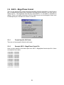
1
Vespa – RFPulse User Manual and Reference Version 0.2.0 Release date: May 4th, 2011 Developed by: Brian J. Soher, Ph.D. Philip Semanchuk Duke University Medical Center, Department of Radiology, Durham, NC Karl Young, Ph.D. David Todd, Ph.D. University of California, San Francisco Department of Radiology, San Francisco, CA Developed with support from NIH, grant # EB008387-01A1 1 Table of Contents Overview of the Vespa Package ................................................... 4 Introduction to Vespa-RFPulse ..................................................... 5 Case Studies in RF Pulse Design ................................................. 7 Using RFPulse – A User Manual ................................................ 10 1. 2. 3. 4. 5. How to launch Vespa-RFPulse ..................................................................... 10 Quick Guide – The Nuts and Bolts of RFPulse ............................................. 12 The RFPulse Main Window........................................................................... 14 The Pulse Project Window ............................................................................ 15 The Pulse Project Tab................................................................................... 16 5.1 5.2 5.3 6. Management Dialogs .................................................................................... 20 6.1 6.2 7. Loading an existing pulse project ........................................................................17 Running a new pulse project ...............................................................................17 Visualizing Pulse Project Results ........................................................................17 Manage Pulse Project dialog...............................................................................20 Manage Machine Settings Templates dialog.......................................................20 Results Output .............................................................................................. 22 7.1 7.2 Plot results to image file formats .........................................................................22 Plot results to vector graphics formats ................................................................22 Appendix A. RFPulse Design...................................................... 23 A.1 What is under the hood? ............................................................................... 23 A.1.1 Vespa-RFPulse Basic Concepts ........................................................................23 A.1.2 Pulse Projects ....................................................................................................23 Appendix B. RFPulse Transforms............................................... 26 B.1 Basic Info Tab ............................................................................................... 26 B.1.1 Tab Diagram........................................................................................................26 B.1.2 General Usage ....................................................................................................26 B.1.3 Widgets and Parameters .....................................................................................26 B.1.4 Algorithm Applied at Run Time............................................................................27 B.2 SLR Tab (create transformation)................................................................... 28 B.2.1 Tab Diagram........................................................................................................28 B.2.2 General Usage ....................................................................................................28 B.2.3 Widgets and Parameters .....................................................................................28 B.2.4 Algorithm Applied at Run Time............................................................................29 B.3 Hyperbolic-Secant Tab (create transformation)............................................. 31 2 B.3.1 Tab Diagram........................................................................................................31 B.3.2 General Usage ....................................................................................................31 B.3.3 Widgets and Parameters .....................................................................................31 B.3.4 Algorithm Applied at Run Time............................................................................32 B.4 Interpolate-Rescale Tab (general transformation)......................................... 33 B.4.1 Tab Diagram........................................................................................................33 B.4.2 General Usage ....................................................................................................33 B.4.3 Widgets and Parameters .....................................................................................33 B.4.4 Algorithm Applied at Run Time............................................................................33 Appendix C. Third Party Export................................................... 35 C.1 General Functionality .................................................................................... 35 C.2 Siemens-IDEA Format .................................................................................. 36 C.2.1 Format Specific GUI Fields.................................................................................36 C.2.2 Example Siemens-IDEA Output File ..................................................................36 C.3 Siemens-Vision Format ................................................................................. 37 C.3.1 Format Specific GUI Fields.................................................................................37 C.3.2 Example Siemens-Vision Output File .................................................................37 C.4 ASCII – Magn/Phase Format ........................................................................ 39 C.4.1 Format Specific GUI Fields.................................................................................39 C.4.2 Example ASCII – Magn/Phase Output File ........................................................39 3 Overview of the Vespa Package The Vespa package enhances and extends three previously developed magnetic resonance spectroscopy (MRS) software tools by migrating them into an integrated, open source, open development platform. Vespa stands for Versatile Simulation, Pulses and Analysis. The original tools that have been migrated into this package include: GAVA/Gamma - software for spectral simulation MatPulse – software for RF pulse design IDL_Vespa – a package for spectral data processing and analysis The new Vespa project addresses current software limitations, including: non-standard data access, closed source multiple language software that complicates algorithm extension and comparison, lack of integration between programs for sharing prior information, and incomplete or missing documentation and educational content. 4 Introduction to Vespa-RFPulse Vespa-RFPulse is a graphical control and visualization program written in the Python programming language that provides a user friendly front end for calculation of Shinnar-LeRoux (SLR) frequency selective RF pulses, and many other calculations and manipulations. Although RFPulse is meant to be intuitive and is entirely menu-driven, a cursory reading of the information below is recommended. A description of the original MatPulse program (beta version 1.0) is provided in reference 1 (below). The RF pulses and gradient waveforms created by RFPulse follow the general procedures and nomenclature provided in references 2 and 3. Along with SLR based pulses, analytical pulse shapes, such as hyperbolic secant, are also available, as are additional transformation steps such as pulse interpolation and re-scaling. 1. Matson, G.B. An integrated program for amplitude-modulated RF pulse generation and re-mapping with shaped gradients. Magn. Reson. Imaging 12, 1205-1225, 1994. 2. J. Pauly, P. Le Roux, D. Nishimura, and A. Macovski, "Parameter Relations for the Shinnar-Le Roux Selective Excitation Pulse Design Algorithm", IEEE Trans Med Imaging 10: 53 - 65 (1991). 3. S. Conolly, D. Nishimura, A. Macovski, and G. Glover, "Variable-Rate Selective Excitation", J Magn Reson 78: 440 - 458 (1988). What can RFPulse do? 1) Create new RF pulse projects from a list of design algorithms 2) Store pulse projects and their design parameters into a database 3) Re-load previous pulse projects 4) Display pulse results for each step of the design process in a flexible plotting tool 5) Compare side-by-side results from one or more pulse projects 6) Output results in text or graphical format, including MR manufacturer platform formats 7) Export/Import Vespa pulse projects to/from other users 8) Be an open source test bed for your own algorithms and transformations. What is an RF pulse project? A ‘pulse project’ consists of one or more design steps. Each pulse project has a single creation step. You can further refine the pulse by adding additional general transformation steps. Each step of the design process (creation plus other transformations) contains time and frequency domain results for the RF pulse up to that point. These results can be visualized in plots to the GUI at any time. Changes to any given step in the design process trigger a “downstream” calculation of all subsequent transformations. You can open multiple pulse projects and compare them side-by-side. Any pulse project tab can be copied into a new pulse project tab. This allows you to make minor changes to a copy of an RF pulse in order to see the effects on the final results. RFPulse can create (and expects to work with) four separate 'vectors' which you will see mentioned and explained in more detail in later sections: The first, B1, represents an amplitude modulated RF pulse. 5 The second, B2, represents a re-mapped pulse (reshaped for use with shaped gradients). The third, G2, represents the shaped gradient waveform for use with B2. The fourth, F2, represents the frequency offsets for an offset slice (used with B2 and G2). In addition, the constant gradient for a conventional selective pulse is labeled G1. The following chapters run through the operation of the Vespa-RFPulse program both in general and screen by screen. In this manual, command line instructions will appear in a fixed-width font on individual lines, for example: ˜/Vespa-RFPulse/ % ls Specific file and directory names will appear in a fixed-width font within the main text. Online Resources: The Vespa project and each of its applications have wikis with extensive information about how to use, and develop new functionality for, each application. These can be accessed through the main portal at http://scion.duhs.duke.edu/vespa/ 6 Case Studies in RF Pulse Design Note. The following case studies discussion was generously contributed by Dr. Jerry Matson based on the functionality of his MatPulse program. Not all features discussed below are implemented in the Vespa-RFPulse application. Although your MRI instrument has a slew of RF pulses installed and available for use in new experiments, there are many reasons why you may want to consider designing new RF pulses. The figure below shows a generic pulse profile to define terms used to describe a pulse profile. The following sections list some of the reasons why you may want to consider creating your own RF pulse designs. Case 1 – Improved Selectivity Many MRI pulses are designed with short TE sequences in mind, and the pulses are designed with a reduced length (at the expense of increased transition bands which creates some loss in selectivity and sensitivity) to accommodate short TEs. Somewhat longer pulses that provide for shorter transition bands may provide improved S/N for signals with longer T2s. In addition, pulse profiles with minimal transition bands are helpful for slice selection without slice gaps. RFPulse provides menus for designing longer RF pulses to reduce the transition bands. Case 2 – Reduced Contamination Especially for spectroscopy, contamination from signal from outside the excitation bandwidth can be a problem (e.g., leading to lipid or water signals from outside the voxel interfering with spectroscopic signals from within the voxel. Selective pulses designed for improved out-of-band (stopband) suppression can reduce this problem. The SLR pulse design tab in RFPulse allows users to select the amount of stopband (reject band) suppression, and facilitates exploring the tradeoffs involved between increased stopband suppression, increased transition band, and increased pulse length. 7 Case 3 – Observation of Spectroscopic Signals Close to Water Most MRI instruments use Gaussian pulses for water suppression. However, Gaussian-shaped pulses generate large transition zones, leading to suppression of other spectroscopy signals close to water. The use of pulses with improved selectivity (e.g., SLR pulses as designed with RFPulse) can reduce this problem. Case 4 – Lowered Peak Voltage Pulses The peak voltage (or power) that can be applied by the MRI instrument to the coil is limited. This can prevent a desired RF pulse from being implemented on the instrument. For example, spin echo pulses require 3 to 4 times the peak voltage required by a 90 degree pulse producing the same bandwidth. In addition, hyperbolic secant inversion pulses require high peak voltage. There are several approaches to lowering the peak voltage of these pulses. Spin echo pulses: An RF pulse can be expressed in terms of a pair of polynomials, designated A and B (see e.g. the paper by Pauli et al. cited above). For an SLR pulse, the B polynomial represents the magnitude of the selection profile that will result from the pulse, while the A polynomial contains the phase information for the pulse. For a so-called minimum phase pulse, the roots of the A polynomial lie within the unit circle in the complex plane. Reflection of one of the roots of the A polynomial across the unit circle - altering the value of the root from z to 1/(z*) – doesn’t alter the profile produced by the pulse, but may lower the peak voltage required. Typically, the peak voltage can be reduced to around 0.6 of the original voltage required. While the peak voltage is decreased, the price to be paid is that the SAR for the pulse is increased. A second approach to lowering the peak voltage of a spin echo pulse is to use the VERSE technique (see, for example, the paper by Matson cited above), which can be thought of as lengthening the center portion of the pulse to enable the voltage of this section of the pulse to be reduced. The FOCI technique is similar, and can be considered as a particular implementation of the VERSE method. A flexible implementation of the VERSE method is known as ”remapping”. This method enables the RF pulse and associated gradient to be altered to lower the peak voltage of the pulse. While this method does not necessarily increase the overall length of the pulse, depending on the parameters used, it may increase the SAR. Hyperbolic secant inversion pulses: The hyperbolic secant pulse represents an adiabatic pulse, where the performance of the pulse does not change once the total power of the pulse is above a certain threshold. The advantage of this type of pulse is that it can perform well even in an inhomogeneous B1 field. The voltage shape of the hyperbolic secant pulse can be expressed as sech(βτ), where τ is the normalized time extending from -1 to 1. This shape produces a high voltage at the center of the pulse. Garwood et al. have shown that, by using a shape function of the form sech(βτn), the peak voltage of the pulse can be reduced, while the pulse retains its adiabatic character. The original hyperbolic secant pulse is thus designated HS1, while the reduced voltage pulses are designated HSn, where n indicates the power to which τ is raised. RFPulse 8 enables HSn pulses to be designed over a range of values of n. Although larger values of n lower the peak voltage, the selectivity of the pulse is degraded at higher values of n. Case 5 – Reduced SAR Due to the high peak voltage required, both spin echo and hyperbolic secant pulses generate high SAR, and lower SAR versions of these pulses may be desired. For spin echo pulses, the remapping method (discussed in the previous section) can be employed with parameters chosen to lower the SAR (and lengthen the pulse duration) of a spin echo pulse. For a hyperbolic inversion pulse, the pulse can be implemented as an HSn pulse (discussed in the previous section) to lower the SAR. Case 6 – More Exotic Pulses While RFPulse can already be used to create Multiband pulse designs, future additions to RFPulse will include the following: Multiband pulses: in which two separate selection bands are included within a single pulse design. For example, in a spectroscopy editing experiment, editing may be desired simultaneously in two separate regions, or suppression in two regions (e.g., water and lipid). Increased bandwidth pulse designs: useful in spectroscopy to suppress the “two compartment artifact’, which causes signal loss for J-coupled metabolites unless the experiment is conducted with very short TE. Special concatenated RF pulses: used in a variety of experiments. For example, concatenated RF pulses are used in arterial spin labeling experiments such as the TILT experiment and in so-called pseudo continuous arterial spin labeling experiments. B1 insensitive pulse design: particularly at high magnetic field, the B1 field becomes inhomogeneous, and it may be desirable to use RF pulse designs that perform uniform tipping even in the presence of inhomogeneous RF fields. RFPulse provides optimization methods to obtain such designs. 9 Using RFPulse – A User Manual This section assumes Vespa-RFPulse has been downloaded and installed. See the Vespa Installation guide on the Vespa main project wiki for details on how to install the software and package dependencies. http://scion.duhs.duke.edu/vespa. In the following, screenshots are based on running Vespa-RFPulse on the Windows OS, but aside from starting the program, the basic commands are the same on all platforms. 1. How to launch Vespa-RFPulse The usual case: If you installed RFPulse by downloading and unzipping the package and by running “python setup.py install”, then you should already have an icon on your desktop called “RFPulse”. Double clicking on this icon will launch the application. Shown below is the Vespa-RFPulse main window as it appears on first opening. No actual RF pulse project windows are open, only the ‘Welcome’ banner is displayed. Use the RFPulse menu to open an existing pulse project or to create a new project for designing an RF pulse. Shown below is a screen shot of a Vespa-RFPulse session with two pulse project tabs opened side by side for comparison. The functionality of all tools, algorithms and transformation will be described further in the following sections. 10 11 2. Quick Guide – The Nuts and Bolts of RFPulse The creation and modification of RF pulses for use in MR experiments is as much an art as a science. We hope that the modularity and flexibility of design steps as presented in RFPulse will allow and encourage you to play with, and better understand, the effects of changing parameter values in each step of the design. Also, since each step is on a separate tab within the pulse project, you can see the results of each step. To facilitate your initial usage, we offer here a quick description of how to get started using and learning from RFPulse. We start with the assumption that you have already installed and launched the RFPulse application. You should see the Welcome screen displayed with no pulse project tabs displayed. The easiest interaction requires just a few basic steps. From the PulseProject menu, select New to create a new pulse project. In the Basic Info tab, fill in the project name and investigator fields. Select Add Transformations→Create→SLR and a new “SLR” tab appears. Hit the Run button and a time domain RF pulse waveform is displayed in the right panel. (optional) select other plot control options at the bottom of the tab to see other results plots. (optional) vary parameters and hit Run again to observe desired pulse performance. Select PulseProject →Save menu item to store your results to the Vespa database so you can re-open them later. From here you can change parameters on the SLR creation tab to refine the shape, duration or other features of the pulse. You can also select other transformations from the Add Transformations menu. Each transformation appears on a new tab and allows you to further refine your pulse. (The motivations for manipulating RF pulses have been briefly discussed in the Case Studies section). There are two types of transformations, “create” transformations and “general” transformations. As shown above, pulse projects start with a create transformation. Create transformations are the algorithms by which an initial RF pulse is designed (e.g. Shinnar-LeRoux, hyperbolic secant, etc.). Each pulse project has just one create transformation. The create transformations are selected from the Add Transformations→Create menu. General transformations are listed below the Create submenu. General transformations operate on the results of the previous transformation (i.e., the transformation in the tab to the left). Notes 1. Another typical workflow might be to load a saved pulse project from the database, add, edit or delete general transformations, and then save the changed results back to the database. 2. A third typical workflow might be to load a saved pulse project from the database, and copy that into a new pulse project by using the PulseProject→Copy Tab to New Tab menu item. Then modify the RF pulse in the copied tab and compare the results plots to the original pulse project results. 3. Changes can be made to parameter settings in any transformation tab in a pulse project. When you click the Run button, RFPulse calculates the effects of these changes in all 12 transformation tabs “downstream” from the transformation tab changed. Note – as of this writing, there is no “undo” functionality in the transformation tabs in the application. Although, for existing pulse projects that have been loaded into a tab, changes to that project are not saved to the database until you select the PulseProject→Save menu manually. 13 3. The RFPulse Main Window This is a view of the main Vespa-RFPulse user interface window. It is the first window that appears when you run the program. It contains a tabbed window into which pulse projects can be loaded, a menu bar and status bar. One or more pulse projects can be loaded at a time. Each project is displayed in its own tab located at the top of the window. Each project contains input data and results from one pulse project design. As described above, a pulse project is a group of transformation steps that create and modify an RF pulse. Each pulse project tab contains a group of tabs at the bottom of the page that represent the transformations in the project. Transformation tabs contain the input values and results for that step of the pulse design. The pulse project window is initially populated with a welcome text window, but no pulse projects are loaded. From the RFPulse menu bar you can 1) load a previously run pulse project from the Vespa database into a tab, or 2) create a new pulse project and set it up and run it. In either case a tab will appear at the top of the window for each pulse project that is loaded or created. The Management menu allows you to access pop-up dialogs to create, edit, view, delete and import/export pulse projects and Machine Settings (which will be explained fully later). The status bar provides information about where the cursor is located within the various plots and images in the interface throughout the program. It also reports short messages that reflect current processing while events are running. On the Menu Bar PulseProject→New Opens a new pulse project tab. PulseProject →Copy Tab to New This will open a new pulse project tab and populate it with the same values that are listed in the current pulse project. This is a short cut for varying design parameters to get different results while retaining the ability to compare back to a previous results set without having to save them both to the data base. PulseProject →Open Runs the pulse project Browser dialog, from which you can choose a pulse project to open from the database to open. PulseProject →Save Saves the pulse project in the current tab to the database. Note - pulse project results are not automatically saved to data base after a Run button is hit. PulseProject→Third Party Export Opens a dialog that will export the final result of the active pulse project into a file suitable for import to various MR manufacturers’ platforms. PulseProject →Exit Closes current pulse project tab. Will prompt for save if necessary. Add Transforms →Create →SLR Appends an SLR (create transformation) tab to current pulse project 14 Add Transforms →Create →Hyperbolic-Secant Add Transforms →Interpolate and Rescale Management →Manage Pulse Projects Appends an Hyperbolic-Secant (create transformation) tab to current pulse project Appends an Interpolate and Rescale (general transformation) tab to current pulse project. Launches the Manage pulse projects dialog. Allows you to view, clone, delete, import and export pulse projects. Management →Manage Machine Settings Templates Launches the Manage Machine Settings dialog. Allows you to create, edit, view, and delete templates for machine settings information. View→<various> Changes plot options in the selected transformation tab of the active pulse project tab, including: display zero line, turn x-axis on/off or choose units, selecting data type and various output options for all plot windows. Help→User Manual Launches the user manual (from vespa/docs) into a PDF file reader. Help→RFPulse/Vespa Online Help Online wiki for the RFPulse application and Vespa project Help→About 4. Giving credit where credit is due. The Pulse Project Window The pulse project window offers considerable flexibility. You can open multiple projects simultaneously and they can be moved around, arranged and “dockedâ” as desired by left-click and dragging the desired tab to a new location inside the main window. The tabs can be positioned side-by-side, top-to-bottom or stacked. They can also be arranged in any mixture of these positions. The pulse project window can be populated with one or more pulse project tabs, each of which contains the results of one pulse project. Pulse project tabs can be closed using the X box on the tab or with a middle-click on the tab itself. When a pulse project Tab is closed, the pulse project is removed from memory, but can be reloaded from the database at a future time - assuming it was previously saved. 15 5. The Pulse Project Tab A pulse project tab is one page in the pulse project window. Each tab contains one entire pulse project design. A pulse project tab can be used to run a new pulse project and view the results of that design. It can also be used to load an existing pulse project from the database to view results, or to change parameters or other modifications to the pulse project. Each pulse project tab will contain sub-tabs at the bottom of the page that describe the transformations used to design the RF pulse. There will typically be two or more of these “transformation tabs”. The first tab is standard to all pulse projects and is called “Basic Info”. The second tab is always a “create” transformation tab such as “SLR” or “Hyperbolic-Secant” (see Appendix B). Additional tabs, containing “general” transformations such as Interpolate-Rescale (see Appendix B) can be appended after the “create” transformation tab. The pulse project tab can be resized by adjusting the RFPulse application window and each transformation tab has a vertical splitter bar through the middle that can be used to resize the right and left sides. Parameters for each transformation tab are displayed on the left side of the tab, the right side of the tab contains a plotting canvas to visually display the current RF pulse waveform and profile results. Typically, when a transformation tab is added to the pulse project, there are no results to be displayed until the Run button has been clicked. A new pulse project is typically created, set up and run. After this, other changes to parameters can be made and the Project re-run until you are satisfied with the pulse performance. Results from running a pulse project are only saved to the database when specifically requested by you. Transformation tabs are updated to display results after each click on the Run button. If there are transformation tabs “downstream” from the tab where the Run button was hit, the program will automatically propagate changes through those tabs as well (ie. essentially automatically triggering their Run functions). Pulse projects can be modified in any tab multiple times. All saved pulse projects start life as “private”. That means they're only in your database; no one else has seen/accessed them. Once you export a pulse project to share with another user, the pulse project is designated as “public”. That means the pulse project result has been shared with the world. Public objects are “frozen” and become mostly unchangeable. Once a private pulse project has become public, it can never become private again. There are two ways that a public pulse project can be re-used. First, cloning a public pulse project (using the Manage Pulse Projects dialog which is described more fully in Section 6) will create a new, private pulse project in the database with exactly the same properties as the original but with a different name. This clone can then be openend into the pulse project window and modified. Second, any pulse project can be loaded into the pulse project window, whether it is public or private. From there, the Pulse Project→Copy to New Tab menu item will create a new pulse project tab with a copy of the current tab. This copy will be private and ready to be modified. Note that an important difference between cloning and copying tabs is that the clone is automatically saved into the database on creation, while the copied tab is only created in memory until you specifically save it. The View menu on the main menu bar can be used to modify the display of the plots in the active pulse project tab. The resulting modifications only affect the settings in the active pulse project tab. More specifically, only the plot options in the selected transformation tab in the active pulse project tab are affected. These options are preserved as you switch from transformation tab to transformation tab. The following lists the functions on the View menu item: 16 On the Menu Bar View (this menu affects the plots in the currently active PulseProject/Transformation tab) →Show ZeroLine toggle zero line off/on in waveform and profile plots →Xaxis →Show turns off/on vertical grid lines and values along the x-axis →Data Type select Real or Real+Imaginary in waveform and frequency profile plots →Output→<format> writes the plot panel to file as either PNG, SVG, EPS or PDF format 5.1 Loading an existing pulse project The pulse project Browser dialog is launched from Pulse Project→Open menu which is shown below. A list of pulse project names is shown on the left. When a pulse project listed in the browser is clicked on once, its comment and other information are displayed on the right. When the Open button is clicked (or a pulse project’s name is double-clicked on), the program loads the information for that pulse project from the database into a pulse project object in memory. This object then creates a pulse project tab and sets up the transformation tabs that describes its creation. You might notice a delay when opening larger pulse projects. 5.2 Running a new pulse project When you select the Pulse Project→New menu option, a new pulse project tab is created in the pulse project window and the Basic Info transformation tab loaded. This tab requires you to type in a project name before the project can be saved. A project investigator and/or a comment can optionally be added. A list of available transformations is on the Add Transformations menu. Create transformations are found under the Add Transformations →Create sub-menu. All the other transformations directly under the Add Transformations menu are general transformations. A detailed description of each transformation and its general usage can be found in Appendix B. As noted previously, a ‘pulse project’ object consists of one or more transformation objects. Each pulse project object must start with a single create transformation but can contain zero or more general transformation tabs. Each transformation object contains results for that step in the RF pulse design. For more detail on how to get started on creating and manipulating RF pulses, see Section 2 – Quick Guide and the Case Study section on pulse design in this manual. 5.3 Visualizing Pulse Project Results Transformations each contain a plot on the right hand side. This plot can display any (and all) of the five results plots, in any combination, by selecting from the check boxes in the Plot Control 17 panel on the left side of the tabbed window. Turning a check box on or off adds or removes the plot from the figure on the right. You can modify other aspects of the data display from the View menu. The plots displayed in each transformation tab are the cumulative results for all transformation tabs to the left of, and including, the current tab. When a transformation tab is added to a pulse project, RFPulse won't display results until you click the Run button. Changing transformation parameters on the left panel does not typically change the results plotted until after the Run button is hit. On the Plot Control Panel Freq Profile (checkbox) Selects RF pulse frequency profile to be plotted. This result comes from running the RF waveform through the Bloch equations to calculate the complex RF profile at ±1 times the Nyquist frequency and at the calculation resolution set in the Basic Info tab. Abs Freq Profile (checkbox) Selects RF pulse absolute frequency profile to be plotted. The magnitude plot of the frequency profile plot described above. Ext Profile (checkbox) Selects the RF extended frequency profile to be plotted. This result comes from running the RF waveform through the Bloch equations to calculate the complex RF 18 profile at ±4 times the Nyquist frequency and at the calculation resolution set in the Basic Info tab. This allows you to check a wider bandwidth range, albeit at a coarser spectral resolution than for the non-extended profile. This allows you to view out-of-band excitation. Ext-Absolute Profile (checkbox) Selects the RF extended absolute frequency profile to be plotted. This is the magnitude plot of the extended frequency profile plot described above Waveform (checkbox) Selects the time domain RF pulse waveform to be plotted. The Usage Type drop list widget requires a more careful explanation. For any given RF pulse, running the complex time waveform through the Bloch equations results in a description of the magnetization along the Z axis as well as in the X,Y plane. Depending on what the pulse will be used for, you may want to check the pulse performance of either the Mz or Mx,y and sometime both directions. Changing the Usage Type widget allows you to specify what is plotted along the vertical axis (a.k.a. the y-axis) in each plot in the figure. Usage Type effects on Y-axis Choice Excite The Mx (real part) and My (imaginary part, if turned on) magnetization is plotted in all profile plots, with the assumption of initial magnetization along the z axis. Inversion The Mz magnetization is plotted in the real part and zeros in the imaginary part (if turned on) in all profile plots, with the assumption of initial magnetization along the z axis. Saturation The -Mz magnetization is plotted in the real part and zeros in the imaginary part (if turned on) in all profile plots, with the assumption of initial magnetization along the z axis. Spin Echo The Mx (real part) and -My (imaginary part, if turned on) magnetization is plotted in all profile plots, with the assumption of initial magnetization along the y axis The mouse can be used to zoom in on the X and Y dimensions in all plots and to set vertical reference spans along the x-axis. The left mouse button draws a box which designates the region into which to zoom the plot. Click and drag the left mouse button in the window and a yellow box will appear. Drag the mouse to size the zoom box appropriately; release the left button and the plot will zoom into that region. XRange, YRange, plot value, and ΔX and ΔY values will be shown in the status bar while dragging. Click and release the left mouse button in place and the plot will zoom out to its max setting. In a similar fashion, two vertical cursors can be set inside each plot window. Click and drag the right mouse button then release to set the two cursors anywhere in the window. This Cursor Span will display as a light gray span. Click and release the right mouse button in place and the cursor span will be turned off. 19 6. Management Dialogs The Management dialogs allow you to create, delete, edit, import, export or view pulse projects and machine settings templates. These dialogs thus allow you to manage the data in the RFPulse database. It also provides the means for users to share information between themselves via XML files created using the Import/Export functions. Note. 6.1 Manage Pulse Project dialog Access this dialog by clicking on the Management→Manage Pulse Projects menu item. The dialog opens and blocks other activity until it is closed. An example of this dialog is shown in the figure. Pulse project names are listed in the window on the right. You can View, Delete, Clone, Import or Export pulse projects. These functions are summarized below. View: Displays a textual summary of the pulse project. Clone: Copies the currently selected pulse project(s) to a new pulse project with a different unique id and name. The new pulse project is automatically saved in the database. This is typically used on pulse projects that have been designated as “public” in order to have a modifiable copy with which to work. Delete: Removes the selected project(s) from the database. pulse Import: Allows you to select an XML file that contains a pulse project. If the UUID in the file is unique, it is added to the pulse project database. Export: You select a pulse project from the list. A second dialog allows you to browse for the output filename, select if output should be compressed and allows an additional export comment to be typed in. Note that the action of exporting a pulse project (or other objects) caused it to be marked as “frozen” in the database. This means that no changes can be made. This is for the sake of consistency as results are shared. However, a frozen pulse project can still be deleted from the database if needed. This file can be imported into another VespaRFPulse installation using the Import function. If additional changes are desired a new pulse project, cloned from the original “frozen” object, can be created then modified. 6.2 Manage Machine Settings Templates dialog Access this dialog by clicking on the Management→Manage Machine Settings Templates menu item. Actions that can be taken on the dialog include: New, Edit, View, Clone, Set Default and Delete. An example of this dialog is shown below. The "Is Default" column indicates which template is used as the default settings for the machine settings object in a newly created pulse project object. The Set Default button is used to designate the currently selected template as the default template. Only one template can be set as the default at one time. 20 New: A dialog will pop up that gives you a blank form to fill out. Fill in the settings in the widget fields and hit the OK or Cancel button. See the sample in the figure below. Edit: The highlighted metabolite is opened in the machine settings editor. All fields are editable. View: Similar to Edit but no fields are editable. Clone: Select a template in the list, hit clone and a copy of that template is made that is now fully editable. Delete: Deletes selected template(s). Set Default: Used to designate the currently selected template as the default template that sets the machine settings in a new pulse project object. 21 7. Results Output 7.1 Plot results to image file formats Results plots in each transformation tab can all be saved to file in PNG (portable network graphic), PDF (portable document file) or EPS (encapsulated postscript) formats to save the results as an image. The Vespa-RFPulse View menu lists commands that only apply to the active transformation tab in the active pulse project tab. Select the View→Output→ option and further select either the Plot to PNG, Plot to PDF or Plot to EPS menu item. You will be prompted to pick an output filename to which will be appended the appropriate suffix. 7.2 Plot results to vector graphics formats Results in each transformation tab can be saved to file in SVG (scalable vector graphics) or EPS (encapsulated postscript) formats to save the results as a vector graphics file that can be decomposed into various parts. This is particularly desirable when creating graphics in PowerPoint or other drawing programs. At the time of writing this, only the EPS files were readable into PowerPoint. The Vespa-RFPulse View menu lists commands that only apply to the active transformation tab in the active pulse project tab. Select the View→Output→ option and further select either the Plot to SVG, or Plot to EPS menu item. You will be prompted to pick an output filename to which will be appended the appropriate suffix. 22 Appendix A. RFPulse Design A.1 What is under the hood? A.1.1 Vespa-RFPulse Basic Concepts This is a combination of logical concepts and constraints that determine how RFPulse works. These rules are enforced through the application and, to some extent, the database. The main objects in the system are pulse projects, transformations, machine settings and master parameters. There are two types of transformations, “create“ and “general“, which will be described in more detail later. Pulse projects are the primary objects; everything else is secondary. Here's how they're related - Each pulse project has one or more transformations. Transformations are the building blocks of a pulse project design. The pulse project object contains a list of all transformation objects that are part of the RF pulse design. The pulse project also contains the machine settings and master parameter settings used. Each transformation step of the design contains the results of the RF pulse at that step, as well as the parameters used to create that result. The pulse project can be saved at any time, but changes made in the GUI will not be copied into internal objects and thus saved until after the “Run” button is hit (for a given transformation). Each pulse project contains exactly one “create” transformation. This transformation is the first one selected by you, and is positioned as the second transformation tab in the GUI after the standard Basic Info tab. Each pulse project can add any number of general transformations after the create transformation. Each pulse project has only one set of machine settings. Each pulse project has only one set of master parameters. We expect users to share data via RFPulse’s export and import functions. For this reason, the RFPulse pulse project object has a universally unique id (UUID) . Machine settings used in a given pulse project are stored in that project when it is exported and are thus available when imported. A.1.2 Pulse Projects Pulse projects are the main focus of the RFPulse application. A Pulse Project’s raison d'etre is to help you design an RF pulse through a series of transformation steps. These transformations first create and subsequently modify an RF pulse to achieve the desired results. This set of transformations is the pulse project’s transformation list. 23 Currently, that list is implemented as a linear group of transformation objects. The first transformation object is always Basic Info. This is a special transformation object in that it occurs prior to any RF pulse waveform results being created. This object modifies meta-data within the pulse project and sets up global parameters that can affect pulse creation/modification algorithms in subsequent steps. Specifically, it allows you to select the Machine Settings and Master Parameters for the pulse design. The second transformation is always a create transformation that implements an RF pulse design algorithm, such as ShinnarLe Roux or hyperbolic-secant, that creates an initial RF pulse waveform result. Subsequent steps always contain a general transformation which uses the waveform result of the previous step as an input to be modified by the current transformation step. The transformation design was selected to allow more modularity in RF pulse design and increased flexibility in the display of intermediate results. Each transformation tab in the pulse project has a manageable number of parameter widgets in its GUI. These can be modified and applied to the local set of results without having to run all previous steps. Results are plotted in the transformation tab to allow you to visually inspect the effects of their settings for each design step. The figure below is a visual representation of two steps in the transformations that make up an imaginary pulse project. Each transformation contains the parameters used in its algorithm, a set of results from running its algorithm, and a reference to the results in the previous transformation step (used as an input). Transformations can be added or removed from the pulse project, typically by closing the associated tab in the GUI, with a few caveats. New transformation steps can only be added to the end of the current project. Any general transformation can be closed/removed, however this triggers an automatic recalculation of the steps “downstream” of that transformation. The create transformation can not be removed unless all general transformations have been previously closed/removed. This is due to the fact that the general transforms would have no results on which to act without an initial create transformation. The take-home lesson from this section is that the Vespa-RFPulse application provides a modular design platform for optimizing RF pulses. Various steps in RF pulse creation and modification can be included in a given design, or not. In the appendix that follows, we will specify what each transformation step included does, are and how they are typically used. Other useful information: 24 • Anytime a tab’s GUI is out of sync with the parameter values used for the last Run of the transformation, the tab’s name will contain an asterisk (‘*’) next to it. Hitting Run will clear this. 25 Appendix B. RFPulse Transforms This section provides some basic information about the transformations (both “create” and “general” types) available in the RFPulse application. A description of the user interface and the parameters that can be set for each transformation is given. A brief overview of the algorithm applied when the Run button is hit is also presented. B.1 Basic Info Tab B.1.1 Tab Diagram B.1.2 General Usage This is a special transformation tab, neither “create” nor “general” type, which you must always fill in so that RFPulse can correctly identify the pulse project to/from the database. The name field MUST be filled in before the pulse project can be saved to the database. B.1.3 Widgets and Parameters Name – text, must be a unique text string within the group of pulse project names in the database Investigator – text, (optional) UUID and Created – not editable, just given FYI Machine Settings – label, listing the name of the currently selected machine settings. Edit – button, opens an editable dialog that displays the current machine settings for modification. 26 Calculation Resolution – integer, the number of points used in the Bloch equation calculations to create pulse profiles. More points result in a more finely sampled bandwidth but at the expense of longer calculation times. Bandwidth Type – droplist B.1.4 Algorithm Applied at Run Time There is no Run button on this tab. To proceed to the next step you select a “create” transformation from the Transformation→Create menu. 27 B.2 SLR Tab (create transformation) B.2.1 Tab Diagram B.2.2 General Usage This is a “create” transformation tab. The SLR tab provides for creation of computer optimized SLR shaped (amplitude-modulated) RF pulses typically denoted as B1. B.2.3 Widgets and Parameters Tip Angle – float, effective tip angle of the pulse in degrees. As of this writing, this parameter is limited to shallow tip angles (just above zero, e.g. 0.001, to 30 degrees), 90 degree, or 180 degree angles. Note that the pulse is shaped for the specified tip angle. To see the effect of the pulse at the wrong power (that is, producing the wrong tip), the pulse must be re-scaled and the profile recalculated with the Bloch Equations. Time Steps – integer, number of steps in the pulse. The number of pulse steps is usually selected in powers of two to speed the calculations. The profile shape is not improved by increasing the number of steps beyond around 128. However, the smoothness of the pulse (and minimization of out-of-band effects) is improved with more steps. For 90 degree pulses the minimum number of steps recommended is 64, while for 180 degree pulses the recommended minimum is 128. Note that the calculations are more rapid for a small number of steps (e.g., 64 steps), and a larger number of steps may be selected after the other pulse parameters have been decided upon. Duration – float, in milliseconds, total time of the pulse. Values selected may not be achievable due to the minimum dwell time and dwell time increment set in the machine settings. In this case, an achievable value will be suggested. 28 Bandwidth – float, in kHz, width of the pass band in kHz as measured at full width half max amplitude value. Separation – float, in kHz (optional). This control is only activated if Dual Band is selected. This is the separation in kHz between the two passbands as measured at full width half max amplitude values. Single or Dual Band – radio button, sets whether one or two passbands will be included in the design of the pulse. Single Band produces conventional slice-selective pulses. The Dual Band selection can be used to produce a dual band pulse such as a dual band saturation pulse. Non-Coalesced Phase Type – dropbox, selections ‘linear’, ‘max’ or ‘min’. Refocused (i.e. linear phase pulse) is generally preferred for an excitation or spin echo pulse, while Max Phase or Min Phase are preferable for inversion or saturation pulses Filter – radio button, selects whether the SLR algorithm uses a Remez or least-squares optimization algorithm. Passband Ripple – float, in percent, of the RF pulse profile. See notes below in ‘Reject Ripple” Reject Ripple – float, as a percent of the RF pulse profile amplitude. These ‘ripple’ parameters are used to estimate a transition band, which is the parameter actually used in the calculations. Although the ripple estimates are quite accurate for 180, 90, and very shallow tip pulses, they would be in error for pulses calculated at intermediate angles B.2.4 Algorithm Applied at Run Time When you hit the Run button … The following description is based on content from the “Handbook of MRI Pulse Sequences, Bernstein MA, Kevin F, King KF, Xiaohong JZ, Academic Press, 2004”. The SLR algorithm was developed to solve the difficult inverse problem of finding what RF pulse to apply, given a desired slice profile and the initial condition of the magnetization. For small flip angles, the shape of an excitation pulse can be approximated by an inverse Fourier transform of the slice profile but this approximation breaks down for pulses in the range of 30-90° or larger. Iterative numerical optimization methods can be used for large tip angles, but the SLR method allows for a direct, non-iterative solution in certain situations. Characteristics such as RF bandwidth, pulse duration, tip angle, percent ripple in the passband, and percent ripple in the stopband can be specified as well as acceptable tradeoffs between these parameters. The algorithm returns the exact RF pulse through a straightforward computational process. The SLR algorithm uses two key concepts: The SU(2) group theoretical representation of rotations and the hard pulse approximation. Two typical ways of describing rotations in three-dimensional space are: 1) via 3 x 3 orthogonal rotation matrices and 3 x I vectors, i.e. via the special orthogonal 3D group SO(3) 2) via 2 x 2 unitary matrices, and 2 x 1 complex vectors called spinors, i.e. via the special unitary group SU(2) (Pauly et al.1991). These two representations are completely equivalent ways of describing macroscopic rotations such as those experienced by the magnetization vector. But the SU(2) representation offers considerable mathematical simplification, and as a result is used in the SLR algorithm. The second important conceptual component of the SLR algorithm is the hard pulse approximation (Pauly et al. 1991), which is useful in particular in the case of non-adiabatic pulses. The hard pulse approximation states that any shaped, or soft, pulse B1(t) can be approximated by a series of short hard pulses followed by periods of free precession. The larger the number of hard pulses used, combined with the resultant decrease in the duration of the free precision periods, the more accurate the approximation. 29 By describing rotations in the SU(2) representation and using the hard pulse approximation, the effect of soft pulses on the magnetization vector can be mathematically described by two polynomials with complex coefficients. The mathematical process that converts an RF pulse into the two polynomials is called the ‘forward SLR transform’. It is important that the inverse SLR transform also can be calculated. The inverse transform yields the RF pulse, given the two complex polynomials corresponding to the desired magnetization. In digital signal processing (DSP), these polynomials are filters for which there are well-established and powerful design tools available. In the SLR algorithm, the inverse SLR transform is used in conjunction with finite impulse response (FIR) filter design tools to design RF pulses directly (Pauly et al. 1991). Vespa-RFPulse uses these DSP tools to turn user input parameters into the appropriate complex polynomials and apply the inverse SLR transformation to generate a corresponding RF pulse. 30 B.3 Hyperbolic-Secant Tab (create transformation) B.3.1 Tab Diagram B.3.2 General Usage This is a “create” transformation tab. B.3.3 Widgets and Parameters Total Rotation – float, in degrees, Time Steps – integer, number of steps in the RF pulse Dwell Time or Bandwidth – float, microseconds or kHz, respectively. Either the bandwidth or the dwell time must be provided (when one parameter is given, the other is automatically calculated). However, the width or dwell time calculations are only approximate Cycles – float, number of cycles before truncating pulse. Power(n) – integer, power of hyperbolic secant function Sharpness(mu) – float, parameter that defines the sharpness of the function Filter Type – droplist, apodization filter type – Hamming or Cosine Filter Application – float, percentage, how much to apply the filter (0.0 to 100.0) 31 B.3.4 Algorithm Applied at Run Time When you hit the Run button … Hyperbolic secant pulses are adiabatic pulses that are typically used for inversion and are relatively insensitive to inhomogeneities in the B1 field and transmitter power setting, and result in very uniform frequency profiles. For adiabatic pulses both the amplitude and frequency of the pulse are typically varied. The pulses are adiabatic in that the amplitude is large enough and the frequency variation is slow enough (the adiabatic condition) that the longitudinal magnetization follows the direction of the effective magnetic field generated by the combined B0 and B1 fields. More specifically the adiabatic condition is that the precession of the magnetization vector about the effective field vector is more rapid than the change in angle of the effective field vector. For a hyperbolic secant inversion pulse the initial effective field is aligned with B0 and the final effective field is aligned in the opposite direction. Hyperbolic secant pulses have the remarkable property that once B1 is strong enough, inversion is achieved over a frequency selective range (slice) such that further increases in B1 do not result in increases in flip angle. Due to the frequency dependent phase that is generated by a hyperbolic secant pulse, they can not be used as refocusing pulses. A disadvantage of hyperbolic secant pulses and adiabatic pulses generally is that they typically involve high SAR, though as described in the case studies section above there are techniques for lowering the SAR associated for a given hyperbolic secant pulse. Hyperbolic secant pulses constitute one of the few analytic solutions of the Bloch equations (Silver MS, Joseph RI, Hoult DI, “Selective spin inversion in nuclear magnetic resonance and coherent optics through an exact solution of the Bloch-Riccati equation”, Phys Rev A, 1985, Apr;31(4):2753-2755.) and are actually solitons (yes, this is a real word) or non-dispersive solutions. For power(n)=1 they have the form: where A(t) is the modulated, time dependent amplitude and (t) is the modulated, time dependent frequency, and and are parameters. For the form of higher order hyperbolic secant functions see Tannus A and Garwood M, “Improved Performance of Frequency-Swept Pulses Using OffsetIndependent Adiabaticity”, 1996, J. Mag. Resonance, A 120 133-137. RFPulse takes the specified user input parameters and generates a hyperbolic secant pulse of the above form. 32 B.4 Interpolate-Rescale Tab (general transformation) B.4.1 Tab Diagram B.4.2 General Usage This is a “general” transformation tab. B.4.3 Widgets and Parameters Interpolate – checkbox, turns Interpolation algorithm on/off. Current Dwell Time – float, the dwell time from the previous results, i.e. the results from the previous transformation (or tab). If there are no previous results, then this value will be zero. New Dwell Time – float, the target dwell time for the interpolation. If this new dwell time violates the minimum dwell time or the dwell time increment (set in the Machine Settings), an error is reported. Rescaling – checkbox, turns Rescaling algorithm on/off. On Resonance Tip – float, equal to the new value for either the net rotation or total rotation. B.4.4 Algorithm Applied at Run Time When you hit the Run button … 33 Interpolate will perform a linear interpolation to recalculate the waveform. The new dwell time will be used to create the time axis, and the number of time points will be changed to span the duration - up to the last point. The interpolation routine is performed in one direction and assumes the points are at the beginning of each time slice. For data points added after the last point in the waveform, the last B1 value will be used (extended). Rescaling changes the on-resonance tip angle (either the net tip angle or the total tip rotation) of the pulse by rescaling the amplitude of the pulse. Net angle is calculated as: (integral of the waveform)*gamma Total rotation is calculated as: (integral of the absolute value of the waveform)*gamma The choice of net tip angle or total tip rotation is determined by this rule: If the sum of the absolute values of the imaginary components of the waveform (B1) is greater than 0.01, then it uses the total rotation, otherwise it uses net angle. For analytic pulse types (e.g. the Hyperbolic-Secant) rescaling can be used to change the amplitude of the pulse for various magnetic fields, by changing the total rotation significant amounts if needed. Amplitude modulated pulses (e.g. SLR pulses) can only be adjusted by a few percent before they start to degrade in performance. In this case, rescaling can be used to see how much it degrades, so one can see how it performs under various intensities - that may be caused by susceptibility issues, limitations in the field coils, etc. Note: For amplitude modulated pulses (such as an SLR pulse) the tip angle specified on the interpolation and rescaling transformation widget (the on-resonance tip) is the tip angle at the center of the profile. However, due to ripples in the passband, the tip angle at the profile center is usually at an extremity (either maximum or minimum) of the allowed tip angle as specified by the ripple amplitude set by the user when the pulse was designed. Thus, the tip angle at the center of the profile may be different from the tip angle used for the design of the pulse. This, however, does not invalidate the initial design, which provides for the correct average tip angle over the profile for which the pulse was created. 34 Appendix C. Third Party Export This section describes the Third Party Export dialog launched by selecting the PulseProject→ThirdPartyExport… menu item. This dialog converts RFPulse waveform results into various third party formats and exports the converted results to a file. At the moment, RFPulse supports three formats: 1) Siemens IDEA single RF pulse ASCII format. 2) Siemens Vision single RF pulse ASCII format. 3) Generic ASCII magnitude/phase representation. The same dialog is used to output all formats; an example is shown below: C.1 General Functionality The third party export dialog acts on the pulse project that is active when the dialog is launched. The GUI reformats itself depending on the selection in the Format pull down list. All formats save ONLY the waveform result from the last transformation tab in the project. Specify the file to which you wish to export results by clicking the Browse… button. This selection is used slightly differently in each format. The Output Location typically defaults to the last location where something was saved. The differences in default file names will be discussed specifically for each format in the sections below. Parameters specific to the format are listed in the next sections (if any) and are also described more fully below. 35 C.2 Siemens-IDEA Format The Siemens Pulsetool utility can import RF pulse or gradient waveforms that are saved in the ASCII file format described in the Siemens IDEA manual. Typically, only one RF pulse or gradient waveform is stored in each file. At the moment, only RF pulses are exportable from the RFPulse application. The first figure in this section shows the Third Party Export dialog configured for the Siemens-IDEA format output. C.2.1 Format Specific GUI Fields Siemens-IDEA format ASCII files have some user-set and automatically-calculated parameter header lines at the top of the file. These lines are followed by magnitude-phase value pairs, one pair per line, for each time step in the RF waveform. We refer you to the Siemens IDEA manual for more specific details for each automatically-calculated header parameter. User-set header parameters that are required include: Name (text) This value defaults to the pulse project name, but can not contain spaces or periods, so these are replaced by underscores automatically. This value is also used as the default filename for the output location. Comment (text) The default comment contains the pulse project name, UUID, and pulse duration as reminders to you once it is imported into IDEA. This also allows the “Name” header variable and/or filename to be changed without losing provenance regarding the pulse project origin of this result. This comment is contained on only one line in the output file, so don’t hit return in entering your comment. Min Slice Thickness (float, [mm]) See the Siemens IDEA manual for additional description of this parameter. Vespa-RFPulse defaults this value to 1.0. Max Slice Thickness (float, [mm]) See the Siemens IDEA manual for additional description of this parameter. Vespa-RFPulse defaults this value to 40.0. C.2.2 Example Siemens-IDEA Output File Here is a short example of the data output to a Siemens-IDEA format output file. Note that the COMMENT parameter is typically all on a single line but formatted here for easier reading. PULSENAME: COMMENT: Simple_64pt_SLR Exported from Vespa-RFPulse project name = Simple 64pt SLR, UUID = a1cec249-446c41e2-a2fd-578a3894ad7d, and pulse duration = 8.0 [ms] REFGRAD: 0.000003670 MINSLICE: 1.000000000 MAXSLICE: 40.000000000 AMPINT: 8.436948615 POWERINT: 7.329981263 ABSINT: 12.869012534 0.043329947 0.026630458 0.029410526 0.027636394 0.020032857 0.006048280 0.014027609 0.038877678 0.066164780 0.092508011 0.114093901 3.141592654 3.141592654 3.141592654 3.141592654 3.141592654 3.141592654 0.000000000 0.000000000 0.000000000 0.000000000 0.000000000 ; ; ; ; ; ; ; ; ; ; ; (0) (1) (2) (3) (4) (5) (6) (7) (8) (9) (10) … 36 C.3 Siemens-Vision Format This is a format that is compatible with older Siemens MR scanners. The code for this format was derived from Jerry Matson’s MatPulse program rather than directly from Siemens documentation. Many of the fields are the same (and have similar meaning) as those for Siemens-IDEA format. C.3.1 Format Specific GUI Fields Siemens-Vision format ASCII files have some user-set and automatically-calculated parameter header lines at the top of the file. These lines are followed by magnitude-phase value pairs, one pair per line, for each time step in the RF waveform. We refer you to the Siemens Vision documentation for more specific details for each automatically-calculated header parameter. User-set header parameters that are required include: Name (text) This value defaults to the pulse project name, but can not contain spaces or periods, so these are replaced by underscores automatically. This value is also used as the default filename for the output location. Comment (text) The default comment contains the pulse project name, uuid, and pulse duration as reminders to you once it is imported into IDEA. This also allows the “Name” header variable and/or filename to be changed without losing provenance regarding the pulse project origin of this result. This comment is contained on only one line in the output file, so don’t hit return in entering your comment. Family Name (text) This value is used to group related pulses in the Siemens-Vision pulse libraries. It may not contain spaces or periods. Min Slice Thickness (float, [mm]) See Siemens Vision documentation for additional description of this parameter. Vespa-RFPulse defaults this value to 1.0. Max Slice Thickness (float, [mm]) See Siemens Vision documentation for additional description of this parameter. Vespa-RFPulse defaults this value to 40.0. C.3.2 Example Siemens-Vision Output File Here is a short example of the data output to a Siemens-Vision format output file. Note that the Entry_Description parameter is typically all on a single line but formatted here for easier 37 reading. Also the waveform results are entered sequentially, one value per line, all magnitude values first followed by the phase values. Begin_Entry: VESPA_RFPulse_Generated_Pulse Entry_Type: 6 Pulse_Name: Simple_64pt_SLR Entry_Description: Exported from Vespa-RFPulse project name=Simple 64pt SLR, UUID=a1cec249-446c-41e2-a2fd-578a3894ad7d, and pulse duration = 8.0 [ms] Num_Points: 64 Family_Name: vespa Slice_Thick_Min: 1.000000000 Slice_Thick_Max: 40.000000000 Reference_Grad: 0.000003670 Power_Integral: 7.329981263 Ampl_Integral: 8.436948615 Envelope_Mode: 1 Entry_Values: 0.043329947 0.026630458 0.029410526 0.027636394 0.020032857 0.006048280 0.014027609 0.038877678 0.066164780 0.092508011 0.114093901 0.127025923 0.127717372 0.113967653 0.085044517 0.042370597 0.010457088 0.067715754 … 3.141592654 3.141592654 3.141592654 3.141592654 3.141592654 3.141592654 0.000000000 0.000000000 0.000000000 0.000000000 0.000000000 0.000000000 0.000000000 0.000000000 0.000000000 0.000000000 3.141592654 3.141592654 … 38 C.4 ASCII – Magn/Phase Format This is a very simple ASCII output format that basically writes the waveform to a text file as a pair of magnitude and phase terms (expressed as floating point numbers). One time point is written per line. The magnitude term has been normalized to 1.0, and phase is expressed in radians. There is no header information in this file format so you are encouraged to name each file descriptively as a reminder as to what is in each file. C.4.1 Format Specific GUI Fields There are no format specific fields for this format. C.4.2 Example ASCII – Magn/Phase Output File Here is a short example of the data output to an ASCII – Magn/phase format output file. Values are separated by a space. 0.043329947 0.026630458 0.029410526 0.027636394 0.020032857 0.006048280 0.014027609 0.038877678 0.066164780 0.092508011 0.114093901 0.127025923 0.127717372 0.113967653 0.085044517 0.042370597 0.010457088 0.067715754 3.141592654 3.141592654 3.141592654 3.141592654 3.141592654 3.141592654 0.000000000 0.000000000 0.000000000 0.000000000 0.000000000 0.000000000 0.000000000 0.000000000 0.000000000 0.000000000 3.141592654 3.141592654 … 39