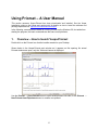
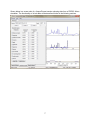
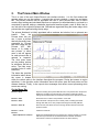
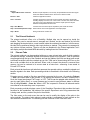
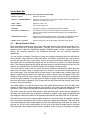
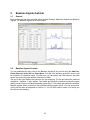
1
Vespa – Priorset User Manual and Reference Version 0.8.1 Release date: July 17th, 2014 Developed by: Brian J. Soher, Ph.D. Philip Semanchuk Duke University Medical Center, Department of Radiology, Durham, NC Karl Young, Ph.D. David Todd, Ph.D. University of California, San Francisco Department of Radiology, San Francisco, CA Developed with support from NIH, grant # EB008387-01A1 1 Table of Contents Overview of the Vespa Package ................................................... 3 Introduction to Vespa-Priorset....................................................... 4 Using Priorset – A User Manual .................................................... 6 1. 2. Overview – How to launch Vespa-Priorset ...................................................... 6 The Priorset Main Window .............................................................................. 8 2.1 The Priorset Notebook .......................................................................................... 9 2.2 Priorset Tabs ......................................................................................................... 9 2.3 Mouse Events in Plots ......................................................................................... 10 3. Spectral Settings Sub-tab ............................................................................. 12 3.1 General ................................................................................................................ 12 3.2 Metabolite Spectral Settings Section ................................................................... 13 3.3 Dataset Noise Settings Section ........................................................................... 14 4. Metabolite Signals Sub-tab ........................................................................... 15 4.1 4.2 5. Baseline Signals Sub-tab .............................................................................. 16 5.1 5.2 6. General ................................................................................................................ 15 Metabolite Signals Parameters............................................................................ 15 General ................................................................................................................ 16 Baseline Signals Controls ................................................................................... 16 Results Output .............................................................................................. 17 6.1 8.2 6.3 Plot results to image file formats ......................................................................... 17 Plot results to vector graphics formats ................................................................ 17 Simulated Data Output to File ............................................................................. 17 2 Overview of the Vespa Package The Vespa package enhances and extends three previously developed magnetic resonance spectroscopy (MRS) software tools by migrating them into an integrated, open source, open development platform. Vespa stands for Versatile Priorset, Pulses and Priorset. The original tools that have been migrated into this package include: GAVA/Gamma - software for spectral simulation MatPulse – software for RF pulse design IDL_Vespa – a package for spectral data processing and analysis The new Vespa project addresses current software limitations, including: non-standard data access, closed source multiple language software that complicates algorithm extension and comparison, lack of integration between programs for sharing prior information, and incomplete or missing documentation and educational content. 3 Introduction to Vespa-Priorset Vespa-Priorset is application written in the Python programming language that allows users to create simulated MR data sets. Vespa-Priorset allows users to: 1) Select from existing Vespa-Simulation Experiment in the Vespa database. 2) Specify a single set of Experiment loop parameters (if more than one) on which to base the priorset’s metabolite basis functions. 3) Specify the spectral resolution as the bandwidth and number of points in the FIDs. 4) Scale individual metabolite areas. 5) Create a Voigt lineshape envelope that has a specific Ta/T2 value for each metabolite and a global Tb/T2* value for the entire priorset. 6) Add unlimited Gaussian spectral peaks with independent area, ppm, linewidth and phase to create simulated metabolite baseline signals. 7) SNR can be set using an independent reference line (not included in spectrum) to maintain RMS noise levels even as metabolite line shape changes. 8) Output to Vespa-Analysis compatible data format or a simple text/binary header/data format. 9) Output a single simulated spectrum or an array of spectra, containing the same signal model but different noise, for use in Monte Carlo evaluations. What is a Priorset? A ‘Priorset’ consists of a simulated MR spectroscopy (MRS) data set that has be created using prior information from a Vespa-Simulation Experiment. The combination of “prior information data set” has been shortened to “priorset” in this manual. A priorset can only contain metabolites from a single set of loop parameters from the Experiment. On output, the priorset contains header information about all signals, processing and noise that were performed to create the data. What is the Priorset Notebook? This is the main window of the Priorset application. It contains one or more tabs, each of which contains the data and processing for an entire priorset. Multiple priorsets can be created/loaded as tabs in the Priorset notebook. Priorsets are created in three steps, organized as three sub-tabs in each Priorset tab. These sub-tabs are ‘Spectral Settings’, ‘Metabolite Signals’, and ‘Baseline Signals’. Upon output, a full provenance for sub-tab parameters is created as part of the Priorset XML output data format. A variety of graphical and text-based methods are available for saving results, as well. The following chapters run through the operation of the Vespa-Priorset program both in general and widget by widget. In this manual, command line instructions will appear in a fixed-width font on individual lines, for example: ˜/Vespa-Priorset/ % ls Specific file and directory names will appear in a fixed-width font within the main text. 4 Online Resources: The Vespa project and each of its applications have Trac Wiki sites with extensive information about how to use, and develop new functionality for, each application. These can be accessed through the main portal site at http://scion.duhs.duke.edu/vespa/ 5 Using Priorset – A User Manual This section assumes Vespa-Priorset has been downloaded and installed. See the Vespa Installation guide on the Vespa main project wiki for details on how to install the software and package dependencies. http://scion.duhs.duke.edu/vespa. In the following, screenshots are based on running Priorset on the Windows OS, but aside from starting the program, the basic commands are the same on all platforms. 1. Overview – How to launch Vespa-Priorset Double click on the Priorset icon that the installer created on your Desktop. Shown below is the Vespa-Priorset main window as it appears on first opening. No actual Priorset windows are open, only the ‘Welcome’ banner is displayed. Use the Priorset → Open Priorset menu to open saved priorsets into tabs, or the Priorset → New Priorset from Experiment menu to create a new priorset. 6 Shown below is a screen shot of a Vespa-Priorset session showing data from a PRESS 144ms simulation. The functionality of all sub-tabs will be described further in the following sections. 7 2. The Priorset Main Window This is a view of the main Vespa-Priorset user interface window. It is the first window that appears when you run the program. It contains the priorset notebook, a menu bar and status bar. The priorset notebook can be populated with one or more priorset tabs, each of which contains input settings and simulated data from one priorset. As described above, a priorset is a comprised of spectral settings, metabolite signals and baseline signals, each of which has its own sub-tab in the respective priorset tab. Sub-tabs are organized along the bottom edge, while priorset tabs are organized along the top edge. The priorset Notebook is initially populated with a welcome text window, but no priorsets are loaded. From the Priorset menu bar you can 1) open a priorset that has previously been processed by Priorset and then saved into the Priorset VIFF XML format, or 2) create a new priorset. In either case a tab will appear for each priorset that is opened or imported. The View menu items set the plotting options for whichever sub-tab is active. The Help menu provides links to useful resources. The status bar provides information about where the cursor is located within the various plots in the interface throughout the program. During plot zooms or region selections, it also provides useful information about the cursor start and end points and the distance between. Finally, it also reports short messages that reflect current processing while events are running. On the Menu Bar Priorset→Open Opens an existing VIFF priorset XML file into a new priorset tab in the priorset Notebook. The state of the priorset as it was saved, including all sub-tab settings and simulated data, are restored as the priorset is opened into its tab. Priorset →New Allows the user to create a new priorset in a new Tab. Priorset →Save Saves the state of the priorset as it currently exists, including all sub-tab settings and data, into a VIFF (Vespa Interchange File Format) XML file. Priorset →Save As Same as Save, but allows the user to change the file name into which the priorset is saved. Priorset → Close Closes the active tab. Priorset →Export Spectrum <various> Writes the simulated data from the priorset out to various formats. For formats that allow it, provenance for the simulated data is included. Otherwise. Provenance is saved to a separate text file in the same directory. 8 Priorset →Export Monte Carlo <various> Similar to Export Spectrum, but an array of spectral data with the same signal model, but different added noise is saved out to various formats. Priorset →Exit Closes the application window. View→<various> Changes plot options in the plots on each sub-tab of the active priorset tab, including: display a zero line, turn x-axis on/off or choose units, select the data type (real, imag, magn) displayed, and various output options for all plot windows and experiment in text format. Help→User Manual Launches the user manual (from vespa/docs) into a PDF file reader. Help→Priorset/Vespa Online Help Online wiki for the Priorset application and Vespa project Help→About 2.1 Giving credit where credit is due. The Priorset Notebook The priorset notebook offers a lot of flexibility. Multiple tabs can be opened up inside the window. They can be moved around, arranged and “docked” as the user desires by left-click and dragging the desired tab to a new location inside the notebook boundaries. In this manner, the tabs can be positioned side-by-side, top-to-bottom or stacked. They can also be arranged in any mixture of these positions. There is only the one Notebook in the Priorset application, but it can display multiple simulated MRS data sets by loading them into Priorset tabs. 2.2 Priorset Tabs The priorset notebook can be populated with one or more priorset tabs, each of which contains the spectral settings, metabolite signals and baseline signals of one priorset. Tabs for priorsets are arranged along the top of the notebook and can be grabbed (left-click and drag) and moved to different locations inside the notebook as you like. Tabs can be closed using the X box on the tab or with a middle-click on the tab itself. When a tab is closed, the priorset is removed from memory, but can be restored to its current state at a future time - assuming it was saved to Priorset VIFF format. Each priorset tab has three sub-tabs that represent the spectral settings, metabolite signals and baseline signals in the data. Each processing sub-tab is described in more detail in the following section. Priorsets are only saved to file when specifically requested by the user. On selecting Priorset → Save, the current state of the priorset, ie. all settings and results in all tabs, is saved into a file in the Vespa Interchange File Format, or VIFF. This file can be updated when desired by the user by again hitting Save, or a new filename can be used to save different states in different files by using Priorset → Save As. When a VIFF file is opened in Priorset, all tabs and results are restored to the state they were in upon save. Each processing sub-tab displays name of the Simulation Experiment that provides the basis functions for the metabolites, the indices of the specific Experiment set of loop parameters that is being used, and the y-scale of the plot in the sub-tab. The View menu on the main menu bar can be used to modify the display of the plots in the active sub-tab. The state of plot options in each sub-tab is maintained in each sub-tab as the user switches between them. The following lists the functions on the View menu item: 9 On the Menu Bar View (this menu affects the plots in the currently active Priorset tab) →ZeroLine→Show toggle zero line off/on →ZeroLine→Top/Middle/Bottom display the zero line in the top 10% region, middle or bottom 10% region of the canvas as it is drawn on the screen →Xaxis →Show display the x-axis or not →Xaxis→PPM/Hz x-axis value in PPM or Hz →Data Type select Real, Imaginary, or Magnitude spectral data to display →Plot Views→Final/All Three select whether only the final simulated spectrum is displayed, or the final spectrum, the metabolite signals and baseline signals are each displayed in their own plot. →Output Experiment Text displays the selected Experiment object in text format in a separate text editor, similarly to what can be displayed in the Vespa-Simulation application. →Output→View→<various> writes the entire plot to file as either PNG, SVG, EPS or PDF format 2.3 Mouse Events in Plots Most processing sub-tabs have plots in their right hand panels. These plots may contain one or more axes which may change dynamically. Typically, the Priorset plot will show either one spectrum which is the sum of metabolite signals + baseline signals + noise, or three plots which display the summed spectrum, the metabolite spectrum and the baseline spectrum, respectively. You can control a number of functions by using your mouse interactively within the plot area of most sub-tabs. Vespa-Priorset is best used with a ‘two-button’ mouse that has a scroll wheel, but can also work fine with a ‘two-button’ mouse, as most mouse-driven features for the scroll wheel also have a corresponding widget that can be clicked on or typed in to cause the same effect. The following describes the typical actions that can be effected using the mouse in a plot window. Any variations from this will be noted in the following sub-tab sections. The mouse can be used to set the X-axis and cursor values in sub-tab plots. When there are three plots, the same X-axis or cursors are set on all three. The left mouse button sets the Xaxis zoom range. Click and hold the left mouse button in the window and a vertical cursor will appear. Drag the mouse either left or right and a second vertical cursor will appear. PPM value changes will be reflected in the status bar. Release the mouse and the plot will be redisplayed for the axis span selected. This zoom span will display its range in a pale yellow that disappears when the left mouse is released. Click in place with the left button and the plot will zoom out to its max x- and y-axis settings. In a similar fashion, two vertical cursors can be set inside the plot window. Click and drag, then release, to set the two cursors anywhere in the window. This cursor xpan will display as a light gray span. Click in place with the right mouse button and the xursor span will be turned off. The cursor values are used to determine the “area under the peak” values that are displayed in the status bar. While performing a right-click and drag to create a cursor span the status bar will also display the start/end location of the span and the delta Hz and delta PPM size of the span. The roller bar can be used to increment/decrement the Y-axis scale value. A maximum value for the Y-axis scale is determined the first time a priorset is loaded and displayed. That max value is the value displayed in the scale widget (top right in the priorset) and used when you zoom all the way out. As you roll the ball up/down (or you click on the SpinCtrl widget next to the scale field) the scale value changes and the plot is updated. (Note. It may be necessary to actually 10 click in the plot window to move the focus of the scroll wheel into the plot, before the scroll wheel events will be applied to the Scale value.) Roller balls can typically be used also as a ‘middle button’ but pushing down on it without rolling it up or down. Priorset plots do not make use of events from this middle button. Click and release the left mouse button in place and the plot will zoom out to its max setting. Click and release the right mouse button in place and the cursor span will be turned off 11 3. Spectral Settings Sub-tab 3.1 General Each priorset tab has three sub-tabs called Spectral Settings, Metabolite Signals and Baseline Signals. The Spectral Settings tab is shown below. Theoretical Details The formula below describes how the simulated data signals are created in the time domain as a sum of metabolite M(t), baseline B(t) and noise N(t) functions, and subsequently transformed into the spectral domain using the FFT for display in the Priorset plot panel. The metabolite signal starts with a set of basis functions generated from the a priori Simulation Experiment information. The set of all a priori resonance lines for each metabolite are indexed over n from 1 to Nm. These sinusoids are created at the digital/spectral resolution set by the user. Only the metabolites selected by the user are included. Metabolite basis functions are modified by the user specified area (Am) and T2 decay (Ta) and global frequency shift (ω0), phase 0 (φ0) and T2* decay (Tb) terms. If the ‘Left Shift’ parameter is not zero, then after the time domain FID has been calculated, it is truncated by N integer points (as set by the spectral resolution widget) before being Fourier transformed. The value N is taken from the Left Shift widget setting. 12 3.2 Metabolite Spectral Settings Section The Metabolite Spectral Settings section contains controls that affect the spectral resolution, SNR and global spectral parameters for the simulated data. The data in the plot on the right will update interactively as you change parameters. Spectral resolution and the PPM range of metabolite basis peaks is set by using the Set metabolite spectral resolution and basis PPM range button. This button will launch a dialog (shown below): on which, you can set the Frequency, Spectral Points, Spectral Width and metabolite inclusion range in PPM using spin control widget. Note – changes to any of these widgets will result in a recalculation of all basis functions from the selected Experiment, but not until you hit the OK button. Depending on the number of steps in all Experiment parameter loops, this recalculation can take an appreciable amount of time. However, it does speed up display of different basis sets when the Loop indices change. 13 The Phase 0 and B0 shift widget spin controls set these global values for the simulated data. The Tb spin control is used to set effects of simulated T2* line broadening. An estimate of the resulting Line Width (in Hz) is displayed in the field below. This estimate is based on an assumed Ta (T2) value of 0.3 seconds because each metabolite can have its own T2 value, thus we use this value as a reasonable average. 3.3 Dataset Noise Settings Section The Dataset Noise Settings section contains parameters that affect the amount of noise that is added to each simulated spectrum. The data in the plot on the right will update interactively as you change parameters. Note, the noise displayed is updated every time a parameter is changed, thus low SNR plots will change appreciably each time a parameter changes. Background on SNR calculation Arrays of random noise are created using the numpy.random.randn() method which creates random floats sampled from a univariate “normal” (Gaussian) distribution of mean 0 and variance 1. Two numpy ndarrays of the proper length are combined to create a complex set of random noise samples. The normalized noise is scaled to create a particular SNR setting based on the traditional “peak height divided by RMS noise value” method. In Priorset, the RMS noise is taken directly from the randn() method, but the peak height is measured from a user defined ‘reference peak’ that is set up on the Spectral Settings sub-tab. The reference peak is not plotted as part of the final spectrum. Its definition is used to create a temporary peak at high spectral resolution whose peak height for a given line and sweep width can be measured. This is the peak height used to calculate the SNR value displayed in the Effective SNR field. The reason we use the reference method is that it allows us to keep the same noise scaling factor as metabolite line width changes. Thus we can create priorsets that have the same noise level and the same metabolite areas but at different peak line widths. It also allows users to use a simple definition of SNR in spectra that do not have simple (singlet) lines against which to set an SNR value. The default reference line is a singlet peak with 3 spins (aka. –CH3 group). The user sets the Reference Peak Ta and Tb values to achieve the desired Effective Linewidth value and then scales to the desired SNR level using the Noise RMS Multiplier spin control. Finally, the user can select to turn the noise in the spectrum on/off using the Display noise in the spectrum check box. This is a convenience function only. 14 4. Metabolite Signals Sub-tab 4.1 General Each priorset tab has three sub-tabs called Spectral Settings, Metabolite Signals and Baseline Signals. The Spectral Settings tab is shown below. 4.2 Metabolite Signals Parameters The metabolites included in the spectrum can be selected in two ways. First, as shown in the previous section, a metabolite inclusion range (in PPM) can be set using the ‘spectral resolution’ dialog. Depending on the spectral lines in each metabolite, the metabolite list is repopulated with metabolites that have lines within this range. Second, the user can explicitly select a metabolite for inclusion by clicking on the check box at the start of a line in the metabolite list. Metabolite areas and an intrinsic T2 decay value can be set in each line for each metabolite. The plot to the right displays the spectrum you are designing. The top plot shows the summed metabolite + baseline + noise signals. The middle plot shows the summed metabolite signals (black) overlaid on the individual metabolite signals (blue). The bottom plot shows the summed baseline signals (black) overlaid on the individual baseline signals (blue). You can zoom in/out of this plot the same as described in Section 2.3. You will likely need to zoom in to clearly see the lines you are creating. 15 5. Baseline Signals Sub-tab 5.1 General Each priorset tab has three sub-tabs called Spectral Settings, Metabolite Signals and Baseline Signals. The Baseline Signals tab is shown below. 5.2 Baseline Signals Controls You can add/delete as many lines to the Baseline signals list as you like using the Add Line, Delete Selected, Select All and Select None. Only the lines that have a check in the box will be included in the baseline signal. For each line, you can specify the PPM value for the peak center, the area of the peak and the Gaussian line width. The plot to the right displays the spectrum you are designing. The top plot shows the summed metabolite + baseline + noise signals. The middle plot shows the summed metabolite signals (black) overlaid on the individual metabolite signals (blue). The bottom plot shows the summed baseline signals (black) overlaid on the individual baseline signals (blue). You can zoom in/out of this plot the same as described in Section 2.3. You will likely need to zoom in to clearly see the lines you are creating. 16 6. Results Output 6.1 Plot results to image file formats The plots displayed in all sub-tabs which contain View panels can all be saved to file in PNG (portable network graphic), PDF (portable document file) or EPS (encapsulated postscript) formats to save the results as an image. The Vespa-Priorset View menu lists commands that only apply to the active Priorset tab and selected processing sub-tab. Select the View→Output→ option and further select either Plot to PNG, Plot to PDF or Plot to EPS item. The user will be prompted to pick an output filename to which will be appended the appropriate suffix. 8.2 Plot results to vector graphics formats The plots displayed in all sub-tabs which contain View panels can all be saved to file in SVG (scalable vector graphics) or EPS (encapsulated postscript) formats to save the results as a vector graphics file that can be decomposed into various parts. This is particularly desirable when creating graphics in PowerPoint or other drawing programs. At the time of writing this, only the EPS files were readable into PowerPoint. The Vespa-Priorset View menu lists commands that only apply to the active Priorset tab and selected processing sub-tab. Select the View→Output→ option and further select either Plot to SVG, or Plot to EPS item. The user will be prompted to pick an output filename to which will be appended the appropriate suffix. 6.3 Simulated Data Output to File The simulated data can be output to file in a number of formats. In all cases you will be prompted to select a director/filename for the output. Use the Priorset→Export Spectrum and Priorset→Export Monte Carlo menu items to select if you want to output just the single spectrum shown on the plot, or if you want Priorset to create an output file with multiple spectra consisting of copies of the pure metabolite + baseline signals with different noise signals. Use the Voxels in Dataset spin control on the Spectral Settings sub-tab to indicate how many voxels to create in the Monte Carlo output file. Note, in a Monte Carlo output file the data will be stored as a two dimension data set. with Spectral points and Voxels in Dataset spin control values as the dimensions. Both single spectrum and Monte Carlo priorsets can be output to VIFF (Vespa Interchange File Format) Raw Data format. In both cases, the data output is time domain (k-space) data. The VIFF Raw Data format is importable into Vespa-Analysis and has the added benefit of being able to store a full provenance of the creation of the simulated data in its XML hierarchy. Similarly, both single spectrum and Monte Carlo priorsets can be saved to the VASF (VA San Francisco) file format. This is a simple double file, text header and binary data, format. The *.rsd option will save data (single or Monte Carlo) to file as time domain data. For the single spectrum, you can also select the VASF *.sid option which will save the frequency domain data to file rather than the time domain data. 17