Download Installation and Testing of an Optical Network

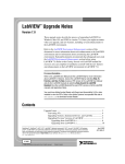
Installation and Testing of an Optical Network
Martha Roseberry
REU Program, The College of William and Mary, Williamsburg, Virgina 23187, USA
(Dated: August 1, 2008)
Abstract
An optical network was installed between two labs to allow the groups to share equipment. The
network consists of five BNC cables and three insulated optical fibers laid between the two labs.
The cables and the fibers were installed, and some testing was done to check the performance of
the optical fiber. The fibers are transmitting light with little power loss. More testing needs to be
done to determine how well the singlemode fibers are maintaining the polarization of the light. As
well as setting up the network, two interfaces for a wavemeter were designed to stream the output
from the wavemeter between the labs.
1
I.
INTRODUCTION
The purpose of this project was to design and install an optical network between Dr.
Novikova’s lab and Dr. Aubin’s lab in the basement of Small Hall. The network would
use BNC cables and optical fiber to allow the labs to transmit electrical signal and light
between the two labs. This will allow the labs to share instruments and lasers, in particular
a Ti:sapph laser for which the labs jointly requested funding. This laser is large and sensitive
to vibrations. Thus, it cannot be moved back and forth between the labs. The optical
network will allow both labs to use the laser. It will also allow the labs to share other
equipment, a wavemeter for example, without having to move them.
II.
OPTICAL FIBER
A.
Types of Fiber
FIG. 1: Diagram of a singlemode fiber. Multimode fibers are built the same way, but have a larger
core diameter, closer to 100 microns. The core must have a index of refraction higher than that of
the cladding to allow for total internal reflection. The buffer layer and the jacket layer are included
on many fiber patchcords to protect the fiber itself.
Optical fibers are long strands of glass or plastic that transmit light due to total internal
2
reflection. The fibers consist of an inner core surrounded by a cladding layer, as shown in
Figure 1. Many fibers also have protective outer coatings. For the fiber to transmit light,
the index of refraction of the core must be greater than that of the cladding.[1]
FIG. 2: The size of the fibercore determines the size of the acceptance cone, the amount and
variability of the light that can be coupled into the fiber.
The core diameter of the fiber determines which wavelengths of light can be transmitted
through the fiber. Only light entering the fiber at appropriate angles will be transmitted
through the fiber. As shown in Figure 2, this creates an a cone of acceptable wavelengths.[1]
In particular, there are two main types of fiber. Those with cores large enough to accept
multiple modes of light are called multimode fibers, and those with cores so small that they
accept only one mode of light are called single mode fibers. The difference between the two
can be seen in Figure 3. Multimode fibers are less expensive and more forgiving to damage.
However, since the light within the fiber can travel along multiple paths, the light that the
fiber outputs may not have the same properties as the light that was inputed. Singlemode
fibers are more delicate and because of their extremely small core diameter, singlemode
fibers are very difficult to couple light into. However, since singlemode fibers allow the light
to travel in only one path, the properties of the outputed light are much more similar to the
properties of the inputed light.[1]
One specific type of singlemode fiber is polarization maintaining fiber. This fiber is
designed to maintain the linear polarization of the light within the fiber. To do this, the
fiber has a non-circular cladding, as shown in Figure 4, that induces a stress on the fiber
core. Thus the fiber core is slightly non-circular as well. Light coupled into the fiber so that
3
core
cladding
FIG. 3: Shown on top is a diagram of a multimode fiber and on bottom is a diagram of a singlemode fiber. Multimode fibers have larger core diameters, approximately 100 microns, and allow
the light to travel along multiple paths. Singlemode fibers have a much smaller core diameters,
approximately 5 microns, and allow the light to travel along only one path.
FIG. 4: Polarization maintaining fibers have a non-circular cladding. The main types of polarization maintaining fibers are PANDA fiber, left, and Bowtie fiber, right.
the polarization axes of the light is aligned with either the long or the short axes of the fiber
should maintain its polarization as it travels through the fiber.[2]
The ends of the fibers, though which light is coupled, must be polished. There are two
standard types of polish, Ultra Physical Contact or UPC and Angled Physical Contact, or
4
FIG. 5: UPC polish, top, is slightly rounded to allow for easy coupling, but allows light to reflect
back through the fiber. APC polish, bottom, is polished at an angle which keeps light from
reflecting back.
APC. Flat polishes are used, but can form air pockets when being connected together. With
UPC polish, the end of tip of the fiber is just slightly curved, as shown in Figure 5, which
allows the fibers to connect without an air pocket forming. However, since the connection is
perpendicular to the fiber core, light will reflect back through a fiber that is connected with
UPC polish. To avoid this problem, APC polish is used. With APC polish, the reflected
light reflects at an angle such that it is absorbed in the cladding layer. Fibers with APC
polish are harder to couple into, as the incoming light has to be at the correct angle.[3]
B.
Ordering Fiber
For the optical network several different fibers were needed. From the start of the project,
it was known that one multimode fiber and two singlemode fibers would be needed. After
requesting quotes from several companies, it was determined that OZoptics sold the fiber for
5
the best price and that ThorLabs was the best place from which to buy the couplers. After
the necessary length of the fiber was determined, as described in the Installation section, the
fiber, some barrels, and the couplers were ordered. The three fibers that were ordered were
one multimode fiber, item name MMJ-3AF3AF-IRVIS-100/140-3-45, one singlemode fiber
optimized for light with a wavelength of 633nm, item name PMJ-3AF3AF-633-4/125-3-45-1,
and one singlemode fiber optimized for incoming light with a wavelength of 850nm, item
name PMJ-3AF3AF-850-5/125-3-45-1. All of the fibers were polished with angled polish
and had the standard fixed connection or FC couplers.
III.
A.
INSTALLATION
Determining the Path of the Fiber
Before installing the fiber, it was necessary to determine the best path between Dr.
Novikova’s lab and Dr. Aubin’s lab. An initial thought was to take the most direct path
between the two by laying the fiber along the outside wall, see Figure 6. This could not be
done because of the staircase which was between the two labs. Instead, it was decided that
the best path for the fiber would be to take the fiber along the hallway. The ceiling above
the hallway was both easy to access and a relatively clear space to lay the fiber without
obstacles. Now that the general path had been decided upon, it was necessary to determine
the exact length of fiber necessary. The fiber needed to reach all points of the optics tables
in both labs. Also, it was desirable for the fiber to only make right angles. The calculation
was done several times, and the length of the path, as shown in Figure 6, was approximately
37 meters. This includes 10 feet in each lab for the fiber to reach from the ceiling to the
optics tables. The final length of fiber ordered was 45 meters, to allow for slack room along
the path and in the labs.
B.
Installing the BNC
Before we installed the fiber, long coax or BNC cables were installed along the same
path. The BNC cables were needed, but they also served as a test for how to install the
fiber, which is much more delicate. The BNC cables were first untangled and measured to
be about 43 meters long. There were 10 of these cables, and it was determined that only
6
Novikova
Aubin
restrooms
stairs
small hallway
main hallway
FIG. 6: Diagram showing the two labs. The red line represents the path of the network cables and
fibers. The dashed blue line shows a path for the fibers what was considered but rejected. The
black ovals show the places where the fiber passes through holes in walls. The small black box
represents the position of an electrical box along the network path.
five needed to be installed. These five cables were bundled together. The other five were set
aside for whenever they are needed.
Installing the BNC was easier than expected. The large coil of cable was left in the
hallway outside Dr. Novikova’s lab. Then one end was shuffled down to Dr. Aubin’s lab.
There were only a few tricky spots along the way. The obvious one was the wall into Dr.
Aubin’s lab. Two holes were drilled into the lab, one for the fiber and one for the BNC
cable.
Another problem was the wall into the small hallway outside of Dr. Aubin’s lab. This
wall already had a hole, which was lucky, but it was small, hard to get to and had rough
edges. With the BNC cable, however, it was possible for just one person to feed it through
from the big hallway, and only occasionally go to the other side to check that it was coming
through alright.
The third obstacle was the power box about halfway down the hallway. It was not very
difficult to lay the BNC cable around the electrical pipes.
The last obstacle was the wall into Dr. Novikova’s lab. This wall already had a very
large hole in it, but the wall itself is 18 to 24 inches wide, and because of the angle from
which it is accessible, the actual reach from the hallway to the lab is about 3 feet. Thus,
the wall cannot be simply reached across. For the BNC cable this problem was solved by
using a meter stick to push the end of the cable into the lab. Then the cable was fed into
7
the ceiling and pulled into the lab.
Installing the BNC cable was not difficult and took one day to complete. It also demonstrated what places were likely to be problem spots when installing the fiber. However, the
solutions used for getting around these problem spots put more strain on the BNC cable
than it would be possible to put on the optical fiber.
C.
Installing the Fiber
Each of the three optical fibers was installed separately, but each was done in the same
way. The fiber was layed out slightly differently than the BNC cable. The BNC cable was
heavy, and therefore the main bundle of BNC had been left in place while the ends were
moved. Optical fiber cannot be strained, and therefore cannot be pulled, so this was not a
good solution for installing the fiber. However, the fiber is very light and small, so the main
bundle of each fiber was carried along the path and uncoiled along the way.
Since it was the cheapest, the multimode fiber was installed first. Fifteen meters of the
fiber were measured and bundled to be left in Dr. Novikova’s lab. The bundle was wrapped
in bubble wrap to protect it, and then both the spool and the bundle were taken into the
hallway. With the aid of a second person and a meter stick, the bundle was passed through
the hole in the wall of Dr. Novikova’s lab and enough slack was let off the spool to allow
the bundle to sit on the top shelf near the wall above the soldering table. This being done,
while moving slowly down the hallway the fiber was carefully unrolled from the spool and
laid in place.
The first obstacle was the power box. In the case of the BNC it was easy to pull the
cables around the box and the electric pipes. However, the opening through the pipes was
not large enough for the spools on which fiber came. Thus, at this point along the hallway
the fiber was unrolled from the spool and wrapped into a coil. The coil could then pass
though the opening between the electric pipes. It was convenient to leave the fiber on the
spool until this point because already a significant amount of the fiber had been laid and
the relatively short amount which had to unwound was easier to keep from tangling.
After taking the fiber off the spool and going around the electric pipes, the fiber was
carefully laid around the corners at the end of the hallway, as shown in the Figure 6. At
this point, it was necessary to pass the fiber through the small hole into the small hallway
8
outside Dr. Aubin’s lab. The hole was too small for the entire bundle of fiber to be passed
through at once, so the fiber was fed through the hole. This required two people, one to
carefully feed the fiber through the hole from the main hallway, and one to carefully gather
it on the other side in the small hallway.
Once the fiber was in the small hallway all that remained was to feed it though the hole
already drilled in the wall of Dr. Aubin’s lab. The fiber was carefully navigated around the
various pipes that run along the small hallway, and then stung over to hole in the wall of Dr.
Aubin’s lab. Before feeding it though the hole, a small piece of the insulation was put into
the hole. The insulation fit, but it was a tight fit and this was done now so that the fiber
would not be damaged trying to do it later. Then the fiber was fed through the hole and
allowed to hang down into Dr. Aubin’s lab. In the lab, the fiber was allowed to hang and
bundle itself when it reached the floor. However, several times during this process I checked
to make sure the fiber was not knotting itself or getting caught on anything inside the lab.
This same procedure was done with the two single mode fibers after the multimode fiber
was successfully installed.
D.
Installing the Insulation
With the fiber installed, all that remained was to install the insulation and then route the
fiber to where it was needed inside both labs. The insulation used was typical copper pipe
insulation that appears to be a black, foam tube with a slit cut along it. The insulation we
used had adhesive along the slit so that once the insulation was in place, the plastic covering
the adhesive could be removed and the tube could be glued shut. The straight pieces of
insulation were easy to install, for the most part. The slit in the insulation was opened by
hand and the fibers carefully placed inside, then the insulation tubes were sealed shut. To
go around corners pieces of straight insulation were bent by hand and a heat gun was used
to slightly melt the inside of the bend. This way the insulation would stay at least partially
bent.
Insulation was installed along the path of the fiber starting in the hallway near Dr.
Novikova’s lab. To put insulation across the wide wall of Dr. Novikova’s lab, a piece
of insulation was placed around the fibers and then slid carefully along until it crossed the
wall. Then insulation was installed along the hallway in long straight pieces. Each additional
9
piece of insulation was duct taped to the previous to ensure that the entire path was well
insulated. Also, as the fiber was being insulated cable ties were used to attach the insulated
fiber to the electrical pipes that ran along the wall.
Along the main hallway I had only one problem with putting up the insulation. About
halfway down the hallway the three fibers had been laid so that the two singlemode fibers
were on one side of an ethernet cable and the multimode fiber was on the other. To insulate
all three fibers, the ethernet cable was also put inside the insulation for one section of the
insulation. This section should be easy to identify, as the ethernet cable come out of the
section a few inches from either end.
Two main issues with putting up the insulation happened around the small hole into the
small hallway. These problems were really problems that had occurred when installing the
fiber, but they were not an issue until I tried to install the insulation. In putting the fibers
through the small hole, they had gotten twisted around the BNC cables and one of the fibers
had been laid on the wrong side of a pipe in the small hallway. To fix this, the BNC cables
were taken out of Dr. Aubin’s lab and taken back to the small hole into the small hallway,
but not through it. With the BNC cable here it was possible to untwist the fibers. The fiber
that was incorrectly laid was also taken out of Dr. Aubin’s lab and reinstalled correctly.
Once all this had been done, the rest of the insulation into Dr. Aubin’s lab was installed so
that it met up with the small piece of insulation already in place through the hole in the
lab wall. Then the BNC cable was installed back into place.
With the fiber and insulation installed between the labs, the fiber could now be brought
to where it needed to be within the labs. In Dr. Aubin’s lab the fiber needed to run to the
corner of the lab across from where the fiber entered the lab. To do this, the fiber was strung
along the ceiling and insulated as before. The insulated fiber was attached to a pipe running
in the correct direction using cable ties. Once in the appropriate corner, the remaining fiber
was coiled and set on a cable tray until a better method for keeping it is built.
In Dr. Novikova’s lab the fiber was strung along the top of the partition that divides
the lab in two. It was insulated and cable tied in place. This placement of the fiber allows
for the fiber to be easily brought to either optical table without going across the partition.
Once the fiber was in place, the remaining fiber was coiled and put in a box on one of the
shelves attached to the partition.
10
IV.
A.
TESTS AND RESULTS
Testing the Multimode Fiber
The only test performed on the multimode fiber tested the power loss through the fiber.
To put light through the fiber, it was connected to an already aligned multimode fiber in
Dr. Novikova’s lab. The connected used a barrel designed for fibers with angled polish.
The power output from the aligned fiber was 30 mW. To test the power lost through the
barrel, a short fiber was connected to the aligned fiber first, and the power output from
this fiber connection was 26 mW, so approximately 13% of the power was lost through the
barrel. When the long fiber was connected to the aligned fiber, 26 mW of power was still
outputed. Thus, the 13% power loss from the barrel was the only significant power loss and
no significant power was lost through the long multimode fiber.
B.
Testing the Singlemode Fiber
It was necessary to measure the power loss through the singlemode fibers, as well. However, neither lab had an aligned singlemode fiber to which we could connect the network
fibers. Thus, several days were spent aligning a singlemode fiber in Dr. Aubin’s lab. When
the fiber was finally aligned, it had an output power of 4.0 mW. The aligned fiber was then
connected to a short singlemode fiber using a barrel. The output power from this fiber
connection was 3.0 mW. The power through the barrel and the network fiber designed for
850nm was 2.6 mW. The power through the barrel and the fiber designed for 633nm was
3.3 mW. Thus, 25% of the power was lost thought the barrel and the short fiber, 35% lost
through barrel and the 850nm fiber, yet only 17.5% was lost though the 633nm fiber. This
is very surprising because both the aligned fiber and the short fiber were singlemode fibers
designed for 850nm wavelength. However, it appears that both the barrel and the long
network fibers contribute significantly to the power loss.
The singlemode fibers used in the network are polarization maintaining fibers, so we
wanted to know how well they actually maintain the polarization. To do this, we sent the
light output from the fiber through a beam splitter, as shown in Figure 7. The beam splitter
separated the horizontally and the vertically polarized light. The intensity of each path was
measured by a photodetector and viewed on a oscilloscope. A waveplate inserted before the
11
waveplate
photodetector
beam splitter
photodetector
FIG. 7: The output light, red, from the fiber, blue, passes through a waveplate and then through
a beam splitter. The beam splitter separates the horizontally and vertically polarized light and
directs both paths to photodetectors. The output signals from the photodetectors allow us to check
if the polarization of the light is rotating through the fiber.
beam splitter allowed us to adjust the polarization so that equal amounts of light were sent to
each photodetector. If a fiber is maintaining polarization, the output of each photodetector
should be constant and equal. If the polarization is rotating in a fiber, there will be noise
and the signals will not be constant. As one signal increases, the other will decrease.
To maintain polarization, the fibers first needed to be aligned so that the incoming
polarization was aligned with either the long or the short axis of the fiber. Before trying to
align the long network fiber, I found the angles for which the short aligned fiber had minimal
polarization change. The fiber connectors are built with keys, that should be at one of the
axes. In the case of the short singlemode fiber that I had aligned, the key was approximately
at 90 degrees. Thus, I started with a polarization angle of 90 degrees and I took data for
a small range around 90 degrees to determine which angle had the minimum polarization
noise. A plot of this data can be seen in Figure 8. As shown, the best polarization angle
in this case was 95 degrees. Since the polarization can be aligned along either axis of the
fiber, if 95 degrees is well aligned, 5 degrees, 185 degrees and 275 degrees should also be well
aligned. I checked, and this was the case.
After finding the four alignments which minimized the polarization noise for the short
12
8
æ
Intensity Noise HVL
æ
6
æ
æ
æ
æ
4
æ
2
æ
æ
0
80
85
90
95
100
Incoming Polarization Angle
FIG. 8: The noise in the polarization intensities as a function of the incoming polarization angle
for the short 850 nm aligned fiber.
fiber, I used a barrel to connect to the long network fiber. To determine how the polarization
noise changes with the incoming polarization angle, I took data for a range of incoming
angles, measuring the polarization noise for each angle. The data is shown in Figure 9. The
amount of noise fluctuated much more than we expected. It is possible that this structure
is due to the barrel. However, the amount of data taken with just the short fiber was not
taken over a long enough range to determine this. This data was taken for the 850 nm fiber,
but a small amount of data was taken with the 633 nm and it appears to behave similarly.
Although the data from the fiber is unclear, the fiber is well aligned when the incoming
polarization is at 5 degrees. With this incoming angle, the short aligned fiber had a value
∆V /V = 0.4/3.9 = 0.10, where ∆V is the change in the intensity of one polarization signal
and V is the total intensity of one polarization signal when the two signals are equal. For
the long 850 nm fiber, ∆V /V = 0.3/1.69 = 0.18 and for the long 633 nm fiber ∆V /V =
0.3/1.62 = 0.19. However, this data is inconsistent. With a total intensity of 1.69 V, it
would be impossible for the 850 nm network fiber to fluctuate the 6 V shown in Figure 9. I
do not know what caused this inconsistency.
13
6
æ
ææ
æ
Intensity Noise HVL
5
æ
æ
æ
æ
æ
æ
æ
æ
4
æ
æ
ææ
æ
æ
3
æ
æ
æ
æ æ
æ
æ
2
æ
ææ
æ
æ
æ
1
æ
æ
æ
æ
æ
æ
0
0
50
100
150
Incoming Polarization Angle
FIG. 9: The noise in the polarization intensities as a function of the incoming polarization for the
long 850 nm fiber barreled to the aligned 850nm fiber.
V.
TAKING THE NETWORK DOWN
When Small Hall is being remodeled it will be necessary to take the optical network
down. I would suggest two ways of doing this. The first would be to take down all the
insulation first, and then carefully take down the three fibers. The second method would be
to alternately take down a section of insulation and then wind a section of the fibers into
coils. I do not know the best method to remove the insulation, but I would suggest using a
pair of scissors rather than a knife to avoid damaging the fibers inside.
In both cases I think it could be useful to leave the insulation in place in particular places.
These points would be the hole into Dr. Aubin’s lab, the hole into Dr. Novikova’s lab and
the hole into the small hallway. The insulation could be left this these places and the fiber
fed through it while taking the network down. In these places, the fiber has to reach over
rather rough walls where it could get caught. The insulation will provide a smoother, more
protective path through which the fiber can be pulled or fed. I would not try to pull the fiber
through the entire length of the insulation. The path of the network is long enough that the
three fibers would almost certainly get tangled around each other if this was attempted.
14
VI.
WAVEMETER INTERFACE
Another piece of equipment to be shared between the two labs is a wavemeter currently in
Dr. Novikova’s lab. To use this with the laser in Dr. Aubin’s lab, it is not only necessary to
have the optical fiber to connect the laser to the wavemeter but there must also be a method
for viewing the output of the wavemeter in Dr. Aubin’s lab. With this aim, I created a user
interface for the wavemeter in LabVIEW. This interface is desribed in much greater detail
the user manual written to accompany it, so I will only outline its function here.
There are two versions of the interface. The first uses the LabVIEW web publishing tool
to display an image of the interface on a webpage. This is a simple way to share the data,
but the webpage updates only once about every three seconds. Thus, while this version of
the interface is useful, it could also be very irritating to work with.
The second version of the interface uses the DataSocket server, which is a National Instruments program that is included with LabVIEW. In this case two programs are necessary,
as well as the server. The first program is the writer, which works exactly the same as the internet publishing version of the program only rather than writing to a webpage this program
writes the data to the DataSocket server. The second program is the reader, which simply
reads the data from the DataSocket server and displays it. The reader, writer, and server
can be run on any computer so long as the user provides them with the correct address for
the server.
Both versions of the program can output the wavelength and the power data given by
the wavemeter. The user can select the units in which he/she wants to view the data, and
can choose the medium through which the laser is traveling. Also, both programs allow the
user to save the data, along with the time, to a user specified file.
VII.
CONCLUSION
The BNC cables and the three fibers were successfully installed. The fibers were insulated
and routed to appropriated places in both labs. In testing the fibers, the multimode fiber does
not appear to have significant power loss. The singlemode fibers do appear to have significant
power loss, but the percentage is not known. However, the singlemode fiber does seem to
be losing no more power than was expected. When testing the polarization maintaining
15
ability of the fiber, we found that the fiber can be aligned to minimize the polarization
rotation, but further analysis needs to be done to determine how the polarization noise
varies with the incoming polarization angle. So, the optical network has been installed and
is working. However, still more testing can be done on the fibers to determine how well they
are performing after being installed.
[1] Wikipedia: Optical fiber, http://en.wikipedia.org/wiki/Fiber optics, accessed July 29, 2008.
[2] Wikipedia: Polarization-maintaining optical fiber, http://en.wikipedia.org/wiki/Polarizationmaintaining optical fiber, accessed July 29, 2008.
[3] Timbercon: Photonic design at the speed of light, http://www.timbercon.com/, accessed July
29, 2008.
16