Download AA-600 AA-1000 AA-1400

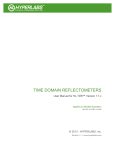
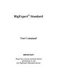
RigExpert®
AA-600
Antenna Analyzer
0.1 to 600 MHz
AA-1000
Antenna Analyzer
0.1 to 1000 MHz
AA-1400
Antenna Analyzer
0.1 to 1400 MHz
User’s manual
2
Table of contents
1. Description ........................................................................................................... 4
2. Specifications ....................................................................................................... 5
3. Precautions........................................................................................................... 6
4. Operation.............................................................................................................. 7
4.1. Preparation for use ......................................................................................... 7
4.2. Turning the analyzer on or off........................................................................ 7
4.3. Main menu ..................................................................................................... 8
4.4. Single- and multi-point measurement modes.................................................. 9
4.4.1. SWR mode............................................................................................... 9
4.4.2. SWR2Air mode ..................................................................................... 10
4.4.3. MultiSWR mode.................................................................................... 11
4.4.4. Show all mode ....................................................................................... 12
4.5. Graph modes ................................................................................................ 13
4.5.1. SWR graph ............................................................................................ 13
4.5.2. R,X graph .............................................................................................. 14
4.5.3. Smith/polar chart.................................................................................... 15
4.5.4. Data screen ............................................................................................ 15
4.5.5. Memory operation.................................................................................. 16
4.5.6. Calibration ............................................................................................. 17
4.6. TDR (Time Domain Reflectometer) mode ................................................... 20
4.6.1. Theory ................................................................................................... 20
4.6.2. Practice .................................................................................................. 23
4.7. Settings menu............................................................................................... 24
4.8. Computer connection ................................................................................... 28
5. Applications ....................................................................................................... 29
5.1. Antennas ...................................................................................................... 29
5.1.1. Checking the antenna............................................................................. 29
5.1.2. Adjusting the antenna ............................................................................ 30
5.2. Coaxial lines ................................................................................................ 30
5.2.1. Open- and short-circuited cables ............................................................ 30
5.2.2. Cable length measurement ..................................................................... 31
5.2.3. Velocity factor measurement ................................................................. 32
5.2.4. Cable fault location................................................................................ 33
5.2.5. Making 1/4-λ, 1/2-λ and other coaxial stubs........................................... 34
5.2.6. Measuring the characteristic impedance................................................. 35
5.3. Measurement of other elements.................................................................... 36
5.3.1. Capacitors and inductors........................................................................ 36
5.3.2. Transformers.......................................................................................... 38
5.3.3. Traps...................................................................................................... 38
5.4. RF signal generator ...................................................................................... 39
3
1. Description
RigExpert AA-600, A-1000 and AA-1400
are powerful antenna analyzers designed
for testing, checking, tuning or repairing
antennas and antenna feedlines.
Graphical SWR (Standing Wave Ratio)
and impedance, as well as Smith/polar
chart displays are key features of these
analyzers which significantly reduce the
time required to adjust an antenna.
Easy-to use measurement modes, as well
as additional features such as connection
to a personal computer make RigExpert
AA-600, AA-1000 and AA-1400
attractive for professionals and hobbyists.
The MultiSWR™ and SWR2Air™ modes
are unique for RigExpert antenna
analyzers.
The built-in TDR (Time Domain
Reflectometer) mode is ideal for locating
cable faults.
The following tasks are easily
accomplished by using these analyzers:
• Rapid check-out of an antenna
• Tuning an antenna to resonance
• Comparing characteristics of an
antenna before and after specific
event (rain, hurricane, etc.)
• Making coaxial stubs or measuring
their parameters
• Cable fault location
• Measuring capacitance or
inductance of reactive loads
4
1. Antenna connector
2. LCD (Liquid Crystal Display)
3. Keypad
4.
5.
6.
7.
8.
Ok button (start/stop
measurement, enter)
Cancel button (exit to main
menu, cancel)
Function button
Power on/off button
USB connector
2. Specifications
Frequency range: 0.1 to 600 MHz – AA-600
0.1 to 1000 MHz – AA-1000
0.1 to 1400 MHz – AA-1400
Frequency entry: 1 kHz resolution
Measurement for 25, 50, 75 and 100-Ohm systems
SWR measurement range: 1 to 100 in numerical mode,
1 to 10 in graph mode
SWR display: numerical or easily-readable bar
R and X range: 0…10000, -10000…10000 in numerical mode,
0…1000, -1000…1000 in graph mode
Display modes:
- SWR at single or multiple frequencies
- SWR, return loss, R, X, Z, L, C at single frequency
- SWR graph, 80 points
- R, X graph, 80 points
- Smith/polar chart, 80 points
- TDR (Time Domain Reflectometer) graph
Optional open-short-load calibration in SWR, R,X or Smith/polar chart graph
modes.
RF output:
- Connector type: N
- Output signal shape: rectangular, 0.1 to 200 MHz. For higher
frequencies, harmonics of the main signal are used.
- Output power: -10 dBm (at 50 Ohm load)
Power:
- Three 1.5V, alcaline batteries, type AA
- Three 1.2V, 1800…3000 mA·h, Ni-MH batteries, type AA
- Max. 3 hours of continuous measurement, max. 2 days in stand-by
mode when fully charged batteries are used
- When the analyzer is connected to a PC or a DC adapter with USB
socket, it takes power from these sources
Interface:
- 320x240 color TFT displaty
- 6x3 keys on the water-proof keypad
- Multilingual menus and help screens
- USB connection to a personal computer
Dimensions: 23·10·5.5 cm (9·4·2”)
Operating temperature: 0…40 °C (32…104 °F)
Weight: 650g (23 Oz)
5
3. Precautions
Never connect the analyzer to your antenna in thunderstorms.
Lightning strikes as well as static discharge may kill the
operator.
Never leave the analyzer connected to your antenna after you
finished operating it. Occasional lightning strikes or nearby
transmitters may permanently damage it.
Never inject RF signal or DC voltage into the antenna
connector of the analyzer. Do not connect it to your antenna
if you have active transmitters nearby.
Avoid static discharge while connecting a cable to the
analyzer. It is recommended to ground the cable before
connecting it.
Do not leave the analyzer in active measurement mode when
you are not actually using it. This may cause interference to
nearby receivers.
If using a personal computer, first connect the cable to the
antenna connector of the analyzer. Then plug the analyzer to
the computer USB port. This will protect the analyzer from
static discharges.
6
4. Operation
4.1. Preparation for use
Open the cover on the bottom panel of the analyzer. Install three fully charged 1.2V
Ni-MH (or three 1.5V alkaline) batteries, watching the polarity.
Do not:
– mix new and old batteries;
– use batteries of different types at the same time;
– overheat or disassemble batteries;
– short-circuit batteries;
– try to re-charge alkaline batteries.
To charge Ni-MH batteries, use charging adapters for this type of batteries. For
longer battery life, it is recommended to use an adapter which charges each battery
separately.
Any leaks of electrolyte from the batteries may seriously damage the analyzer.
Remove batteries if the analyzer is not being used for a long period of time. Store
batteries in a dry cool place.
4.2. Turning the analyzer on or off
To turn the analyzer on or off, use the
(power) button located in the bottom right
corner of the keypad. When this button is pressed, firmware version number as well
as battery voltage are displayed on the LCD.
The on-screen menu system of RigExpert antenna analyzers provides a simple but
effective way to control the entire device.
The analyzer may stay turned on when you connect a cable to its antenna connector (or
when you disconnect a cable). Plug the cable into the antenna connector, and then
tighten the rotating sleeve. The rest of the connector, as well as the cable, should
remain stationary.
Important: If you twist other parts of the connector when tightening or loosening,
damage may easily occur. Twisting is not allowed by design of the N-connector.
7
4.3. Main menu
Once the analyzer is turned on, the Main menu appears on the LCD:
The Main menu contains a brief list of available commands. By pressing keys on the
keypad, you may enter corresponding measurement modes, set up additional
parameters, etc.
Pressing the
(function) key will immediately list additional commands:
There is a power indicator in the top-right corner of the Main menu screen:
• The battery indicator shows battery discharge level. When the battery voltage is
too low, this indicator starts flashing.
• The USB icon is displayed when the analyzer is plugged to a personal computer
or to a DC adapter with USB socket.
RigExpert antenna analyzers are self-documenting: pressing the
(help) key will
open a help screen with a list of available keys for the current mode.
8
4.4. Single- and multi-point measurement modes
In single-point measurement modes, various parameters of antenna or other load are
measured at a given frequency. In multi-point modes, several different frequencies are
used.
4.4.1. SWR mode
The SWR mode (press the
key in the Main menu) displays the SWR bar as well as
the numerical value of this parameter:
Set the desired frequency (the
key) or change it with left or right arrow keys.
Press the
(ok) key to start or stop measurement. The flashing antenna icon in the
(help) key
top-right corner indicates when the measurement is started. Pressing the
will show a list of all available commands for this mode:
9
4.4.2. SWR2Air mode
RigExpert AA-600, AA-1000 and AA-1400 present a new SWR2Air mode which is
designed to help in adjusting antennas connected via long cables.
This task usually involves two persons; one adjusting the antenna and the other
shouting out the SWR value as it changes at the far end of the feedline.
There is an easier way to do the same job by using the SWR2Air mode. The result of
SWR measurement is transmitted on a user specified frequency where it can be heard
with a portable HF or VHF FM radio. The length of audio signal coming from the
loudspeaker of the portable radio depends on the value of measured SWR.
The SWR2Air mode is activated by pressing
+
key combination in the SWR
+
allows setting the frequency to tune the receiver to.
measurement screen.
10
4.4.3. MultiSWR mode
RigExpert AA-600, AA-1000 and AA-1400 have an ability to display SWR for up to
five different frequencies at a time. This mode is activated by pressing
+
key
combination in the Main menu:
(up) and
(down)
You may use this feature to tune multi-band antennas. Use
cursor keys to select a frequency to be set or changed. Press the
key to switch
between SWR bars and numerical representation of this parameter:
Pressing the
(help) key will show a list of other commands.
11
4.4.4. Show all mode
The Show all mode (the
key) will show various parameters of a load on a single
screen. Particularly, SWR, return loss (RL), |Z| (magnitude of impedance) as well as its
active (R) and reactive (X) components are shown. Additionally, corresponding values
of inductance (L) or capacitance (C) are displayed:
This screen displays values for series as well as parallel models of impedance of a
load:
• In the series model, impedance is expressed as resistance and reactance
connected in series:
• In the parallel model, impedance is expressed as resistance and reactance
connected in parallel:
12
4.5. Graph modes
A key feature of RigExpert antenna analyzers is ability to display various parameters of
a load graphically. Graphs are especially useful to view the behavior of these
parameters over the specified frequency range.
4.5.1. SWR graph
In the SWR graph mode (press the
key in the Main menu), values of the Standing
Wave Ratio are plotted over the specified frequency range:
You may set the center frequency (the
key) or scanning range (the
key). By
using arrow keys (
), these parameters may be increased or decreased.
Watch the triangle cursor below the graph.
Press the
(ok) key to start measurement or refresh the graph.
The
key opens a list of radio amateur bands to set the required center frequency and
scanning range quickly. Also, you may use this function to set the whole frequency
range supported by the analyzer.
Press the
key to access a list of additional commands for this mode.
13
4.5.2. R,X graph
In the R,X graph mode (press the
key in the Main menu), values or R (active part of
the impedance) and X (reactive part) are plotted in different colors.
In these graphs, positive values of reactance (X) correspond to inductive load, while
negative values correspond to capacitive load. Please notice the difference in the plots
when series or parallel model of impedance is selected through the Settings menu:
14
4.5.3. Smith/polar chart
The Smith/polar chart (press the
+
key combination in the Main menu) is a
good way to display reflection coefficient over the specified frequency range:
As usual, press the
key for a help screen.
Please notice: Non-US version of analyzers will display Smith chart; a polar chart is
displayed instead on US version.
4.5.4. Data screen
In all graph modes, press
cursor:
+
key combination to display various parameters at
15
4.5.5. Memory operation
In all graph modes, press the
key, and you will be given a choice of 90 memory
) keys, select the desired slot number:
slots. Using arrow up or arrow down (
Press
. You will be prompted to edit the selected memory slot name. Follow
instructions on the display. A new scan will be performed and the data will be saved in
the selected memory slot.
To retrieve your readings from the memory, press then
memory slot number and press
.
To edit names of existing memory slots, press
to edit:
16
+
key, select necessary
and then select the slot number
4.5.6. Calibration
Although RigExpert AA-600, AA-1000 and AA-1400 are designed for high
performance without any calibration, an open-short-load calibration may be applied for
better precision.
The standards used for calibration should be of high quality. This requirement is
especially important for high frequencies (100 MHz and upper). Three different
calibration standards should be used: an “open”, a “short” and a “load” (usually, a 50Ohm resistor). A place where these standards are connected during calibration is called
a reference plane. If the calibration is done at the far end of a transmission line,
parameters of this line will be subtracted from measurement results and the analyzer
will display “true” parameters of a load.
To perform calibration,
1. Enter the SWR graph (the
key), the R,X graph (the
chart (the
+
key combination) mode.
2. Select the desired center frequency and the sweep range.
17
key) or the Smith/polar
3. By pressing the
+
key combination, open the Calibration screen:
key. The analyzer will rescan
4. Connect an “open” to the analyzer and press the
the specified frequency range and save calibration data to its memory.
5. Connect a “short” and press the
key.
6. Connect a “load” and press the
key. Please notice that for displaying the SWR
graph and the Smith/polar chart correctly, the System impedance parameter in the
Settings menu (see page 24) should be same as the actual resistance of the “load”.
After the parameters of all three loads are measures, a “cal” indicator appears at the
bottom of the display:
18
Changing the center frequency or the sweep range will invalidate calibration.
Additionally, pressing the
key in the Calibration screen will invalidate the
key will return the analyzer to the center
current calibration, and pressing the
frequency and the sweep range used during the last calibration:
19
4.6. TDR (Time Domain Reflectometer) mode
4.6.1. Theory
Time domain reflectometers are electronic instruments used for locating faults in
transmission lines.
A short electrical pulse is sent over the line, and then a reflected pulse is observed. By
knowing the delay between two pulses, the speed of light and the cable velocity factor,
the DTF (distance-to-fault) is calculated. The amplitude and the shape of the reflected
pulse give the operator idea about the nature of the fault.
Impulse response:
Instead of a short pulse, a “step” function may be sent over the cable.
Step response:
20
Unlike many other commercially-available reflectometers, RigExpert AA-600, AA1000 and AA-1400 do not send pulses into the cable. Instead, another technique is
used. First, R and X (the real and the imaginary part of the impedance) are measured
over the whole frequency range (up to 600, 1000 or 1400 MHz). Then, the IFFT
(Inverse Fast Fourier Transform) is applied to the data. As a result, impulse response
and step response are calculated.
(This method is often called a “Frequency Domain Reflectometry”, but the “TDR”
term is used in this document since all calculations are made internally and the user can
only see the final result.)
The vertical axis of the resulting graphs displays the reflection coefficient: Γ=-1 for
short load, 0 for matched impedance load (ZLoad=Z0), or +1 for open load. By
knowing the cable velocity factor, the horizontal axis is shown in the units of length.
Single or multiple discontinuities can be displayed on these graphs. While the
Impulse Response graph is suitable for measuring distance, the Step Response graph
helps in finding the cause of a fault.
See the examples of typical Step Response graphs on the next page.
21
22
4.6.2. Practice
Press
+
to open Impulse Response (IR) and Step Response (SR) graphs:
The characteristic impedance and the velocity factor of the cable, as well as display
units (meters or feet) may be changed in the Settings menu.
The
(ok) key starts a new measurement, which will take about a minute. You may
disconnect your antenna or leave it connected to the far end of the cable. This will only
affect the part of the graph located behind the far end of the cable.
Use the arrow keys to move the cursor or to change the display range. Watch the
navigation bar at the top-right corner of the screen to see the current position of the
displayed part of the graph.
The
key will start a new measurement, saving results in one of 10 memory
slots. The
key will retrieve saved data. Use the
+
combination to edit
memory names, if needed.
Pressing
+
opens a data screen which displays numerical values of impulse and
step response coefficients, as well as Z (estimated impedance) at cursor.
The
key will display the help screen, as usual.
23
4.7. Settings menu
The Settings menu (press the
key in the Main menu) contains various settings for
the analyzer. The first page contains the following commands:
– language selection
– backlight brightness and timer
– colour scheme selection
– sound on or off
– go to the second page which contains additional settings
– opens a frequency correction screen, so the output frequency of the
analyzer may be set precisely
– select metric or U.S. units for the TDR display
24
and
– select cable velocity factor for the TDR display
– select system impedance for SWR, Smith/polar chart and TDR displays
– select series or parallel representation (see page 12) for the R,X graph
– go to the third page which contains analyzer self-test options
– RF bridge test. Two filled bars display signal levels at the left and at the
right legs of the resistive bridge. With no load at the antenna connector, the
screen should look like shown on the picture:
For the 50-Ohm load, the filled bars should stand at corresponding positions (notice
the “no load” and “50 Ω” marks):
25
If one of the bars of both bars is not filled at all, the RF output stage or/and the detector
circuits are not working properly in the analyzer:
On the above picture, the first bar indicates no RF signal at one of the legs of the
resistive bridge. Most likely, this means that a high power (such as, from a transmitter)
was injected into the antenna connector and the analyzer was damaged.
– detector output voltage vs. frequency graph. With no load at the antenna
connector, the display should look like shown on the pictures:
26
AA-600:
AA-1000:
AA-1400:
The voltage curve should stay between horizontal lines. The vertical lines are the
bounds of analyzer’s sub-bands.
– bandpass filter frequency response graph. With no load at the antenna
connector, the display should look like shown on the picture:
4
27
The top of the curve should be located in the middle of the screen, between
two horizontal lines. A small horizontal shift of the curve is allowed.
– go to the last page which contains reset commands
– reset the entire analyzer to factory defaults
– delete all graph memories
– go to the last page of the settings menu
4.8. Computer connection
RigExpert AA-600, AA-1000 and AA-1400 antenna analyzers may be connected to a
personal computer for displaying measurement results on its screen, taking screen shots
of the LCD, as well as for updating the firmware.
A conventional USB cable may be used for this purpose. The supporting software is
located on the supplied CD or may be downloaded from the www.rigexpert.com
website. Please see the Software Manual for details.
28
5. Applications
5.1. Antennas
5.1.1. Checking the antenna
It is a good idea to check an antenna before connecting it to the receiving or
transmitting equipment. The SWR graph mode is good for this purpose:
The above picture shows SWR graph of a car VHF antenna. The operating frequency is
160 MHz. The SWR at this frequency is about 1.2, which is acceptable.
The next screen shot shows SWR graph of another car antenna:
The actual resonant frequency is about 135 MHz, which is too far from the desired one.
The SWR at 160 MHz is 2.7, which is not acceptable in most cases.
29
5.1.2. Adjusting the antenna
When the measurement diagnoses that the antenna is off the desired frequency, the
analyzer can help in adjusting it.
Physical dimensions of a simple antenna (such as a dipole) can be adjusted knowing
the actual resonant frequency and the desired one.
Other types of antennas may contain more than one element to adjust (including coils,
filters, etc.), so this method will not work. Instead, you may use the SWR mode, the
Show all mode or the Smith/polar chart mode to continuously see the results while
adjusting various parameters of the antenna.
For multi-band antennas, use the Multi SWR mode. You can easily see how changing
one of the adjustment elements (trimming capacitor, coil, or physical length of an
aerial) affects SWR at up to five different frequencies.
5.2. Coaxial lines
5.2.1. Open- and short-circuited cables
Open-circuited cable
Short-circuited cable
The above pictures show R and X graphs for a piece of cable with open- and shortcircuited far end. A resonant frequency is a point at which X (reactance) equals to zero:
• In the open-circuited case, resonant frequencies correspond to (left to right) 1/4,
3/4, 5/4, etc. of the wavelength in this cable;
• For the short-circuited cable, these points are located at 1/2, 1, 3/2, etc. of the
wavelength.
30
5.2.2. Cable length measurement
Resonant frequencies of a cable depend on its length as well as on the velocity factor.
A velocity factor is a parameter which characterizes the slowdown of the speed of the
wave in the cable compared to vacuum. The speed of wave (or light) in vacuum is
known as the electromagnetic constant: c=299,792,458 meters per second or
983,571,056 feet per second.
Each type of cable has different velocity factor: for instance, for RG-58 it is 0.66.
Notice that this parameter may vary depending on the manufacturing process and
materials the cable is made of.
To measure the physical length of a cable,
1. Locate a resonant frequency by using single-point measurement mode or R,X
graph.
Example:
The 1/4-wave resonant frequency of
the piece of open-circuited RG-58 cable
is 9400 kHz
2. Knowing the electromagnetic constant and the velocity factor of the particular
type of cable, find the speed of electromagnetic wave in this cable.
Example:
299,792,458 · 0.66 = 197,863,022 meters per second
- or 983,571,056 · 0.66 = 649,156,897 feet per second
31
3. Calculate the physical length of the cable by dividing the above speed by the
resonant frequency (in Hz) and multiplying the result by the number which
corresponds to the location of this resonant frequency (1/4, 1/2, 3/4, 1, 5/4, etc.)
Example:
197,863,022 / 9,400,000 · (1/4) = 5.26 meters
- or 649,156,897 / 9,400,000 · (1/4) = 17.26 feet
5.2.3. Velocity factor measurement
For a known resonant frequency and physical length of a cable, the actual value of the
velocity factor can be easily measured:
1. Locate a resonant frequency as described above.
Example:
5 meters (16.4 feet) of open-circuited cable.
Resonant frequency is 9400 kHz at the 1/4-wave point.
2. Calculate the speed of electromagnetic wave in this cable. Divide the length by
1/4, 1/2, 3/4, etc. (depending on the location of the resonant frequency), then
multiply by the resonant frequency (in Hz).
Example:
5 / (1/4) · 9,400,000 = 188,000,000 meters per second
- or –
16.4 / (1/4) · 9,400,000 = 616,640,000 feet per second
3. Finally, find the velocity factor. Just divide the above speed by the
electromagnetic constant.
Example:
188,000,000 / 299,792,458 = 0.63
- or –
616,640,000 / 983,571,056 = 0.63
32
5.2.4. Cable fault location
To locate the position of the probable fault in the cable, just use the same method as
when measuring its length. Watch the behavior of the reactive component (X) near the
zero frequency:
• If the value of X is moving from –∞ to 0, the cable is open-circuited.
• If the value of X is moving from 0 to +∞, the cable is short-circuited.
By using a TDR (Time Domain Reflectometer) mode, even minor discontinuities may
be located in the transmission line.
Example:
The TDR mode shows a visible peak at 1.04 meters, where two 50-Ohm cables
are joined. A peak at 6 meters indicates open-circuit at the end of the cable.
33
5.2.5. Making 1/4-λ, 1/2-λ and other coaxial stubs
Pieces of cable of certain electrical length are often used as components of baluns
(balancing units), transmission line transformers or delay lines.
To make a stub of the predetermined electrical length,
1. Calculate the physical length. Divide the electromagnetic constant by the
required frequency (in Hz). Multiply the result by the velocity factor of the
cable, then multiply by the desired ratio (in respect to λ).
Example:
1/4- λ stub for 28.2 MHz, cable is RG-58 (velocity factor is 0.66)
299,792,458 / 28,200,000 · 0.66 · (1/4) = 1.75 meters
- or –
983,571,056 / 28,200,000 · 0.66 · (1/4) = 5.75 feet
2. Cut a piece of cable slightly longer than this value. Connect it to the analyzer.
The cable must be open-circuited at the far end for 1/4-λ, 3/4-λ, etc. stubs, and
short-circuited for 1/2-λ, λ, 3/2-λ, etc. ones.
Example:
A piece of 1.85 m (6.07 ft) was cut. The margin is 10 cm (0.33 ft). The
cable is open-circuited at the far end.
3. Switch the analyzer to the Show all measurement mode. Set the frequency the
stub is designed for.
Example:
28,200 kHz was set.
4. Cut little pieces (1/10 to 1/5 of the margin) from the far end of the cable until the
X value falls to zero (or changes its sign). Do not forget to restore the opencircuit, if needed.
Example:
11 cm (0.36 ft) were cut off.
34
5.2.6. Measuring the characteristic impedance
The characteristic impedance is one of the main parameters of any coaxial cable.
Usually, its value is printed on the cable by the manufacturer. However, in certain
cases the exact value of the characteristic impedance is unknown or is in question.
To measure the characteristic impedance of a cable,
1. Connect a non-inductive resistor to the far end of the cable. The exact value of
this resistor is not important. However, it is recommended to use 50 to 100 Ohm
resistors.
Example 1: 50-Ohm cable with 100 Ohm resistor at the far end.
Example 2: Unknown cable with 50 Ohm resistor at the far end.
2. Enter the R,X graph mode and make measurement in a reasonably large
frequency range (for instance, 0 to 50 MHz).
Example 1: 50-Ohm cable
Example 2: Unknown cable
35
3. Changing the display range and performing additional scans, find a frequency
where R (resistance) reaches its maximum, and another frequency with
minimum. At these points, X (reactance) will cross the zero line.
Example 1: 28.75 MHz – min., 60.00 MHz – max.
Example 2: 25.00 MHz – max., 50.00 MHz – min.
4. Switch the Data at cursor screen by pressing
previously found frequencies.
+
and find values of R at
Example 1: 25.9 Ohm – min., 95.3 Ohm – max.
Example 2: 120.6 Ohm – max, 49.7 Ohm – min.
5. Calculate the square root of the product of these two values.
Example 1: square root of (25.9 · 95.3) = 49.7 Ohm
Example 2: square root of (120.6 · 49.7) = 77.4 Ohm
5.3. Measurement of other elements
Although RigExpert antenna analyzers are designed for use with antennas and antennafeeder paths, they may be successfully used to measure parameters of other RF
elements.
5.3.1. Capacitors and inductors
Analyzers can measure capacitance from a few pF to about 0.1 µF as well as
inductance from a few nH to about 100 µH.
Be sure to place the capacitor or the inductor as close as possible to the RF connector
of the analyzer.
36
1. Enter the R,X graph mode and select a reasonably large scanning range. Perform
a scan.
Example 1:
Unknown capacitor
Example 2:
Unknown inductor
2. By using left and right arrow keys, scroll to the frequency where X is -25…-100
Ohm for capacitors or 25…100 Ohm for inductors. Change the scanning range
and perform additional scans, if needed.
3. Switch to the Data at cursor mode by pressing
capacitance or inductance.
Example 1:
Unknown capacitor
+
and read the value of
Example 2:
Unknown inductor
37
5.3.2. Transformers
RigExpert analyzers can also be used for checking RF transformers. Connect a 50 Ohm
resistor to the secondary coil (for 1:1 transformers) and use SWR graph, R,X graph or
Smith/polar chart modes to check the frequency response of the transformer. Similarly,
use resistors with other values for non-1:1 transformers.
5.3.3. Traps
A trap is usually a resonant L-C network used in multi-band antennas. By using a
simple one-turn wire coil a resonant frequency of a trap may be measured.
Example:
A coaxial trap constructed of 5 turns of TV cable (coil diameter is 60 mm) was
measured:
A one-turn coil connected to the analyzer was placed a few centimeters away
from the measured trap. The SWR graph shows a visible dip near 17.4 MHz,
which is a resonant frequency of the trap.
38
5.4. RF signal generator
The output signal of RigExpert AA-600, AA-1000 and AA-1400 has rectangular
waveform and level of about -10 dBm (at the 50 Ohm load). Therefore these analyzers
can be used as sources of RF signal for various purposes.
For frequencies up to 200 MHz, first harmonic of output signal can be used. Above 200
MHz, tune your receivers to odd higher harmonics.
Enter the SWR mode or the Show all mode, and press the
output.
(ok) key to start the RF
If needed, use the frequency correction option in the Settings menu (see page 24).
39
Copyright © 2007-2013 Rig Expert Ukraine Ltd.
http://www.rigexpert.com
RigExpert is a registered trademark of Rig Expert Ukraine Ltd.
RigExpert AA-600, AA-1000 and AA-1400
Antenna Analyzers are made in Ukraine.
Printed in Ukraine
23-Oct-2013
40