1
STATISTICAL ANALYSIS ON ENVIRONMENTAL LIMITATIONS
ON THRESHOLD-BASED IRRIGATION MANAGEMENT
by
MARK TODD LUEDECKE, B.S.
A THESIS
IN
STATISTICS
Submitted to the Graduate Faculty
of Texas Tech University in
Partial Fulfillment of
the Requirements for
the Degree of
MASTER OF SCIENCE
Approved
Accepted
May, 1992
II)
f-/J 2:- 7591
to.5
T3
,qq::,
1v'o. I~
~-Z--
l\. "-
Jltc...
..1/1/9:
ACKNOWLEDGMENTS
I would like to thank my committee members, Dr. Truman Lewis,
Dr. Benjamin Duran, and Dr. Hossein Mansouri, not only for their assistance
on this project but also for the education which they provided me.
I would also like to thank the United States Department of Agriculture, specifically Don Wanjura, Dan Upchurch, and James Mahan, for providing the data
for this study.
Most of all, I would like to thank my parents for the financial support and
the encouragement that they gave me throughout my college years.
11
CONTENTS
ACKNOWLEDGMENTS .
11
.lV
LIST OF TABLES
LIST OF FIGURES
v
..
ABSTRACT . . . .
Vll
I. INTRODUCTION: THE EXPERIMENT
II. USER'S MANUAL . . . . . .. .
2.1 Getting Started. . . . . . . . . . . .
2.2 Running the Program
2.2.1 Entering the years . . . . . . .
2.2.2 Entering the types . . . . . . .
2.2.3 Entering the days . . . . . . . . .
2.2.4 Entering the treatments . . . .
2.2.5 Entering the times . . . . . .
2.2.6 Retrieving the data . . . . . .
2.2. 7 Stopping the program . . .
1
5
5
6
6
8
9
11
15
18
19
III. ANALYZING THE DATA . . . . . . . .
3.1 Drybulb versus Wetbulb . . . . . .
3.2 Air versus Canopy . . . . . . . . .
3.3 Analyzing the Data as a Time Series .
3.3.1 Analyzing the Morning Data .
3.3.2 The Noon Data . . . . . . .
3.3.3 The Evening Data . .
3.3.4 An Interesting Result
21
21
24
24
IV. CONCLUSIONS
50
REFERENCES
. . . . . . . . . .
29
37
40
48
51
111
LIST OF TABLES
....
3
1.1
Six treatments with water use and lint yield for 1988.
2.1
Example of an application of program USDA . . . . .
3.1
Correlation analysis between drybulb and wetbulb for 1988
22
3.2
Correlation analysis between drybulb and wetbulb for 1989
25
3.3
Correlation analysis between Air and IRT Temperatures
27
3.4
Data for time series analysis
29
3.5
Results of Model ARMA(0,11)
38
3.6
Results of Model ARMA(0,6)
39
3.7
Results of Model ARMA(18,1)
49
.
.lV
7
LIST OF FIGURES
2.1
Main menu from program USDA.
7
2.2
Year menu from program USDA . .
8
2.3
Type menu from program USDA.
9
2.4
Entering the types for example
2.5
Day menu for program USDA
2.6
Entering the days for 1988
12
2.7
Entering the days for 1989
13
2.8
Entering the days for 1990
13
2.9
Entering the days for 1991
14
10
....
12
2.10 Treatment menu from program USDA
14
2.11 Treatment submenus from program USDA with examples
16
2.12 Time submenu from program USDA
18
2.13 Entering the times for the example
19
3.1
Plot of morning values for 1988
30
3.2
Plot of morning values for 1989
31
3.3
Plot of morning values for 1990
32
3.4
Plot of morning values for 1991
33
3.5
ACF and PACF for 1988
34
3.6
ACF and PACF for 1989
35
3.7
ACF and PACF for 1990
36
3.8
ACF and PACF for 1991
37
3.9
Plot of noon values for 1988
40
3.10 Plot of noon values for 1989
41
3.11 Plot of noon values for 1990
42
3.12 Plot of noon values for 1991
43
v
3.13 Plot of evening values for 1988
44
3.14 Plot of evening values for 1989
45
3.15 Plot of evening values for 1990
46
3.16 Plot of evening values for 1991
47
V1
ABSTRACT
During the past four years (1988-1991), the United States Department of
Agriculture (USDA) performed an experiment testing a theory known as the
Thermal Kinetic Window (TKW) theory. This theory proposes that each species
of crop can have an optimal yield if its canopy temperature can be kept within
a window of temperatures. The main crop of study was cotton which has a
TKW between 23° C and 32° C. An extensive amount of data was collected over
the four years of study. The main purpose of this paper will be to present a
method of extracting certain pieces of this data so that meaningful analyses can
be performed to determine the permissiveness of the environment in allowing the
canopy temperature to remain within the TKW. Some of these analyses will also
be included in this paper.
Vll
CHAPTER I
INTRODUCTION: THE EXPERIMENT
The growth and maturity of cotton varies greatly throughout the season due
to the many environmental characteristics acting upon the crop. Elements such
as wind, radiation, humidity, and air temperature can, in excessive quantities,
affect the growth and maturity of each plant. Due to the fact that these environmental elements are not controllable, theories have been developed which
suggest that certain plant characteristics may be altered in order to aid the plant
to adjust to the environmental factors. Two such characteristics, which have
been a focus of the USDA, are water stress and canopy temperature.
Water stress is a condition in the plant which causes a deficiency of the
requirements needed for proper transpiration in the plant. As the plant is exposed
to both the soil and the atmospheric conditions, the soil moisture level determines
the soil's ability to supply water to the plant depending on the atmospheric
conditions at the time. For example, in areas where the relative humidity is high,
the plant temperature will tend to remain constant with the air temperature, and
in semi-arid areas, such as the Lubbock locale, where the humidity level is usually
around 20-30%, the temperature of the air will usually be 2- 4° higher than
the temperature of the plant. One method that is generally used to determine
whether or not the plant is suffering from water stress is to inspect the foliage
to see if any wilting is present. Another more scientific method is to observe the
canopy temperature (Tc) and the air temperature {T11 ). This method is useful
in determining the level of water stress through the derivation of the crop water
stress index (CWSI) developed by Idso et al. {1981) [3). The CWSI provides an
upper and lower limit for (Tc- T4 ) at any deficit of vapor pressure.
Water stress has proven to be a major criterion in the development of the
cotton during the flowering and boll development stages [1). Through the observation of the canopy temperature, an irrigation schedule was developed that
would adjust the water stress level of the plant. In addition, this irrigation schedule allowed the USDA to test the TKW theory developed by J .R. Mahan et al.
{1987) [2). This theory suggests that if the canopy temperature of the plant was
maintained within the window set for its species, specifically 23° C and 32° C
1
2
for cotton, then the overall yield would be increased with more efficient water
usage. The USDA also theorized that within the TKW there exists an interval
of normalized temperatures (Tn) which the plant tries to maintain when specific environmental conditions are satisfied. The Tn for cotton is between 26° C
and 30° C, and these temperatures became the main focus of the USDA study.
They found that the optimal yield, in relation to fiber length and strength, was
obtained when the Tc was kept within these values.
The USDA was able to observe the Tc through the use of infra-red thermometers (IRT's ). Two IRT's were placed on each of the plots of land, one on the north
side and one on the south side. On each plot of land, there were eighteen 30.5
meter rows of cotton that were spaced 76 em apart and ran from east to west.
One of the advantages to using the IRT's, as opposed to other temperature reading devices, is that the IRT's do not touch the plant at any point which allows
the plant to remain in a natural state. The IRT's read the temperature by inputting the amount of heat and radiation being reflected by the plant. Through
the use of a computer system and the IRT's, the Tc 's were measured every 15
seconds. Then an average of these readings was calculated every 15 minutes and
recorded. These averages were performed twenty-four hours a day, seven days a
week throughout the growing season. Therefore, based on the 15-minute average
readings from the IRT's, the USDA developed the irrigation schedules that would
decrease water stress and, hopefully, improve overall yield.
In order to perform a useful analysis, the USDA set up several plots of cotton,
each receiving a different irrigation schedule. One plot of land was irrigated each
week based on the standard method of observing the soil water profile. If the
profile of the water in the soil was substantially decreased, water was applied
in order to replenish the water level. This treatment will be referred to as the
Soil Water Replacement Fixed (SWRF) treatment and will be used as the control plot. Another plot of land was designed to implement a watering schedule
at variable times depending on when the soil water profile was substantially decreased; however, this method was more lenient than the SWRF treatment. Most
times this plot of land was irrigated every two weeks. This treatment is called
the Soil Water Replacement Variable (SWRV) treatment. Another plot was designed to receive only the initial preplant irrigation and the rainfall thereafter.
3
This treatment will be referred to as the dryland (DRY) treatment. Throughout
the study, at most three plots of land were designed to monitor the periods of
irrigation based on the Tc of the plant. The base temperature varied by 2° C
between each plot of land. If after any 15 minute period, the Tc exceeded the
threshold temperature set for that plot, the irrigation process would begin and
remain on throughout the next 15 minute period. If after the end of that period
the Tc was still above the threshold, irrigation would continue.
In 1988, the three temperature treatments that were studied were 28° C, 30°
C, and 32° C as well as the SWRF, SWRV, and DRY treatments. The following
Table 1.1 gives the final results of each of the six different treatments in terms
of the total water applications and the overall lint yield.
Table 1.1: Six treatments with water use and lint yield for 1988.
I
Trt
28° c
30° c
32° c
SWRF
SWRV
DRY
I H20 applied I Lint Yield I
70 em
46 em
36 em
138 em
75 em
Ocm
1431 ~
1073 ~
1073 ~
1430 ~
1147 !:JL
ha
353 !:JL
ha
After observing the overall yield in comparison to the amount of water applied
to each plot, the USDA came to the conclusion that the 28° C treatment had a
sufficiently greater lint yield [1]. Over the next three years, they concentrated
on temperatures close to 28° C. In 1989, they used 26° C, 28° C, and 30° C as
the temperature treatments. In 1990, they studied only two plots with different
base temperatures, 26° C and 28° C. Finally, in 1991, only the 28° C treatment
was studied as a temperature controlled plot.
Over the four years, an immense amount of data was collected considering
that the temperature readings were recorded every 15 minutes of every day fpr
an average of 150 days each year. So that proper analyses could be performed
on this data, a system was developed that would allow the analyst to extract
4
certain pieces of the data depending on what types of tests were to be analyzed.
The main purpose of this study was to develop such a system through the use of
FORTRAN programs. In the following chapters, an explanation of the programs
and some analyses performed through the use of these programs will be given.
In chapter 2, a user's manual for the main program that actually extracts the
data for analysis is provided with an example, while in chapter 3 there will be
a discussion of some of the analyses performed as well as a discussion of other
programs used in each analysis. Finally, in chapter 4, results of the analyses and
possible future analyses will be discussed.
CHAPTER II
USER'S MANUAL
2.1 Getting Started
Before the program can be run, the user must make sure that the data is
properly set up and in the right directories. For some years, a drybulb and
wetbulb temperature was recorded. However, even though the wetbulb data
may not have been collected for a certain year, the data must appear as if it had
been. During times when some piece of equipment may not have been operating
properly, a missing value number was recorded in place of the bad data. This
number is represented by -99.0 in this study. Therefore, if during some year
the proper amount of data had not been collected, a column of missing values
should be placed into the data set in the respective position. Each data file must
be sixteen columns wide with the first column containing the day of the year.
The second column represents the time of the day beginning with 0 and going
through 2345 in 15 minute intervals. The other fourteen columns will contain
the data with every odd column being the drybulb data, and every even column
the wetbulb data. After each file has been properly formatted, the user must put
the files into their respective directories. The data files should be placed in the
subdirectory corresponding to its year and data type:
\USDA\ 'year'\ 'type'\
For example, the air temperature data from 1988 should be placed into the
\USDA \1988\AIR\
subdirectory.
Each file must also be properly named in order for the program to be able
to locate it. Each file, which contains the data for a certain day, must have the
following format:
5
6
'typeday'.DAT
For example, AIR163.DAT is the air temperature for day 163.
In each instance above, 'type' will be one of the following: AIR, IRT, RAD,
WIN, or CONT. AIR is the air temperature data. IRT is the infra-red thermometer data. RAD is the radiation data. WIN is the wind data, and CONT
is the control data which specifies when the system was actually irrigating. The
'year' will be either 1988, 1989, 1990, or 1991. The 'day' will correspond to the
day that is recorded in that file. The range of days varies from year to year. The
days range from 161-318 in 1988, 171-304 in 1989, 158-297 in 1990, and 155-307
in 1991. Once each of the above conditions has been met, the program will work
properly.
2.2 Running the Program
The program is not required to be in any certain directory; however, it must
be on the same drive as the data, preferably in the root directory. In order to
begin the program, the following command must be entered.
C:\ >USDA< CR >
where USDA is the name of the program, and the < C R > denotes a carriage
return. After a few moments, the main menu will appear on the screen
(Figure 2.1 ). By choosing each of the options available, the user will be able to
extract any portion of data that is desired. Due to the fact that each year is
different with respect to the days recorded and the treatments, Option 1 should
always be selected first.
Throughout the rest of this chapter, the following example will be used in
order to demonstrate the procedures of the program. The data to be extracted
is found in Table 2.1.
2.2.1 Entering the years
At times the user may not want to analyze all of the years, so an option
has been added which allows the operator to analyze either one year or any
combination of years (Figure 2.2).
7
Table 2.1: Example of an application of program USDA
Years
Types
Days
Treatments
Times
1988,1989,1990,1991
AIR,IRT
195-250
drybulb, 28° c
700,1200,1600-1700
MAIN MENU
CODE
FUNCTION
1
Enter the years for analysis
Enter the types for analysis
Enter the days for analysis
Enter the treatments for analysis
Enter the times for analysis
Get the data
Quit
2
3
4
5
6
7
Enter the desired code : _
Figure 2.1: Main menu from program USDA.
H the user chooses to analyze the data within one year (Option 1), he will
then be prompted to enter which year is to be analyzed:
Enter the year for analysis: _
However, if the operator chooses option 2, the program will prompt him to enter
the number of years for analysis and the years. Thus, following the example, the
user will select option 2 and answer the prompts accordingly.
8
YEAR MENU
CODE
FUNCTION
1
2
Perform analysis within a year
Perform analysis among years
Enter the desired code: _
Figure 2.2: Year menu from program USDA.
Enter the number of years for analysis: 4
Enter the year 1 for analysis: 1988
Enter the year 2 for analysis: 1989
Enter the year 3 for analysis: 1990
Enter the year 4 for analysis: 1991
At this time, the program will return to the main menu (Figure 2.1 ).
2.2.2 Entering the types
The user should enter the types of data to be analyzed by selecting option 2.
Upon selecting this option, the operator will receive the following prompt:
Enter the number of types for analysis (1-6): _
This prompt allows the user to extract anywhere from one to six types of
data at a time. After entering the number of types to extract, the output that
will appear on the screen can be found in Figure 2.3. This screen will be shown
as many times as the number of types chosen above.
If for some reason the user enters the same type more than once, the program
will give an error message stating that the type has already been selected and
will ask the user to type a carriage return. The output appears in Figure 2.4.
Again, the program will now return to the main menu (Figure 2.1 ).
9
TYPE MENU
CODE
TYPE
1
Air temperature
Infra-red thermometer
Radiation
Wind
Yield
Irrigation control
2
3
4
5
6
Enter the desired code: _
Figure 2.3: Type menu from program USDA.
2.2.3 Entering the days
The next option to be chosen should be option 3, which allows the user to
specify which days he wants to extract. Upon selecting this option, a. new menu
will appear on the screen giving the user a variety of ways to select the days for
analysis (Figure 2.5, p.12). Again, this menu will appear on the screen as many
times as the number of years chosen. This option has been added in case the user
wants to select different days from each year. The opera.tor can opt to analyze
only one day of the year by selecting option 1, or he can select a number of days
by selecting one of the options 2-4 depending on which suits his needs.
H option 1 is chosen, the following prompt will appear on the screen:
Enter the day for analysis (beg-end): where beg is the first day of the year, and end is the last da.y of the year. H the
user wishes to extract one or more intervals of days, the best option to choose is
option 2 which yields these prompts:
Enter the number of intervals (1-num): _
where num is the number of days in that year for which data was collected.
10
Enter the number of types for analysis (1-6): 2
TYPE MENU
CODE
TYPE
1
Air temperature
Infra-red thermometer
Radiation
Wind
Yield
Irrigation control
2
3
4
5
6
Enter the desired code: 1
TYPE MENU
CODE
TYPE
1
Air temperature
Infra-red thermometer
Radiation
Wind
Yield
Irrigation control
2
3
4
5
6
Enter the desired code: 2
Figure 2.4: Entering the types for example
11
Enter the beginning day of interval i for analysis (beg- end): _
where i is the
i'" interval to be entered.
Enter the last day of interval i for analysis (beg- end): _
H for some reason the days entered are not within the specified interval or if the
beginning and last days are not in the right order, an error message will be given,
and the user will be prompted to start over.
H the user wants to select one day here and there, he should select option
3. In this instance, the program will first prompt for the number of days to be
selected, and then will prompt for the specific days.
Enter the number of days for analysis {1-num): _
where num is the number of days within that year.
Enter the day i (beg-end): _
where i is the i'" day to be entered and beg and end are the first and last days of
the year, respectively.
Finally, option 4 allows the user to select all of the days of the year without
having to enter each day separately. If this option is chosen, the program will
automatically enter the days for each year selected. After the days have been
chosen, the main menu will appear on the screen (Figure 2.1 ).
Since the example extracts the data over all four years, the menu in Figure 2.5
will appear four times on the screen (Figure 2.6, Figure 2. 7, Figure 2.8, and
Figure 2.9).
2.2.4 Entering the treatments
In order to select the treatments for analysis, the user will select option 4
from the main menu (Figure 2.1). Since for some years drybulb and wetbulb
data had been collected, the program will first prompt the user to select which
type of data is to be extracted (Figure 2.10).
12
DAY MENU
CODE
FUNCTION
1
Analyze
Analyze
Analyze
Analyze
2
3
4
one day
succesive days
intermittent days
entire year
Enter the desired code: _
Figure 2.5: Day menu for program USDA
DAY MENU
CODE
FUNCTION
1
Analyze
Analyze
Analyze
Analyze
2
3
4
one day
succesive days
intermittent days
entire year
Enter the desired code: 2
Enter the number of intervals for analysis (1-160): 1
Enter the beginning day of interval 1 (161-318): 195
Enter the last day of interval 1 (161-318): 250
Figure 2.6: Entering the days for 1988
13
DAY MENU
CODE
FUNCTION
1
Analyze
Analyze
Analyze
Analyze
2
3
4
one day
succesive days
intermittent days
entire year
Enter the desired code: 2
Enter the number of intervals for analysis (1-144): 1
Enter the beginning day of interval 1 (171-304): 195
Enter the last day of interval 1 (161-318): 250
Figure 2.7: Entering the days for 1989
DAY MENU
CODE
FUNCTION
1
Analyze
Analyze
Analyze
Analyze
2
3
4
one day
succesive days
intermittent days
entire year
Enter the desired code: 2
Enter the number of intervals for analysis (1-139): 1
Enter the beginning day of interval 1 (158-297): 195
Enter the last day of interval 1 (161-318): 250
Figure 2.8: Entering the days for 1990
14
DAY MENU
CODE
FUNCTION
1
2
Analyze
Analyze
Analyze
Analyze
3
4
one day
succesive days
intermittent days
entire year
Enter the desired code: 2
Enter the number of intervals for analysis {1-152): 1
Enter the beginning day of interval 1 {155-307): 195
Enter the last day of interval 1 {161-318): 250
Figure 2.9: Entering the days for 1991
TREATMENT MENU
CODE
FUNCTION
1
2
3
Analyze drybulb
Analyze wetbulb
Analyze both
Enter the desired code: _
Figure 2.10: Treatment menu from program USDA
I
I
15
After the type of temperature readings have been selected, the program will
prompt the user to enter the number of treatments for the year currently being
considered.
Enter the number of treatments for year (1-tot): _
The treatment submenu for that year will then appear on the screen the same
number of times as selected above. Each of the possible submenus will be demonstrated through the use of the example (Figure 2.11 ).
After the treatments have been entered, the program will return to the main
menu (Figure 2.1)
2.2.5 Entering the times
The final criterion that the user needs to specify is the times of the day that
he wants extracted. This is accomplished by selecting option 5 from the main
menu (Figure 2.1 ). The operator will then have the option to either enter the
times in intermittent intervals or enter the entire day (Figure 2.12).
If option 1 is chosen, the program will prompt for the number of intervals
that will be included in the analysis.
Enter the number of intervals for analysis: _
The next two prompts will ask for the beginning and ending time for the ith
interval. These prompts will be repeated as many times as the time intervals
chosen. If the beginning and ending times for any particular interval are not in
the right order, a run time error will occur, the program will end, and the DOS
prompt will appear. Notice that 1:00 pm is denoted as 1300 not as 100. It is
very important that these numbers are input properly.
Enter the beginning time for interval i (0-2345, 15 min increments): Enter the ending time for interval i (0-2345, 15 min increments): The program will enter all of the times in between the beginning and ending
times provided.
If option 2 is chosen, the program will automatically enter all times starting
16
TREATMENT MENU
CODE
FUNCTION
1
2
3
Analyze drybulb
I
I
Analyze wetbulb
Analyze both
Enter the desired code: 1
Enter the number of treatments for 1988 (1-7): 1
TREATMENT SUBMENU FOR 19881
CODE
FUNCTION
1
28° c
30° c
32° c
Fixed soil water replacement
Variable soil water replacement
Drybase
2 meters (air only)
2
3
4
5
6
7
I
Enter the desired code: 1
Figure 2.11: Treatment submenus from program USDA with examples
from 0 to 2345 without any prompting for the user. Once completed, the main
menu will once again appear on the screen.
Since the example calls for only a few time points, option 2 will be selected.
The user should notice that if only a single time is desired, he will enter the same
time for both the beginning and ending time (Figure 2.13).
17
Enter the number of treatments for 1989 {1-8): 1
TREATMENT SUBMENU FOR 1989
CODE
FUNCTION
1
2
Fixed soil water replacement
28° C treatment 1
28° C treatment 2
26° c
CTV
CTD
2 meters (air only)
3
4
5
6
7
I
I
Enter the desired code: 1
Enter the number of treatments for 1990 {1-6): 1
TREATMENT SUBMENU FOR 1990
CODE
FUNCTION
1
Variable soil water replacement
26° c
30° c
28° c
Fixed soil water replacement
2 meters (air only)
2
3
4
5
6
Enter the desired code: 1
Figure 2.11: (cont.)
I
I
18
Enter the number of treatments for 1991 (1-6): 1
TREATMENT SUBMENU FOR 1991
CODE
FUNCTION
1
7.0 HT
5.5 HT
4.0 HT
4.0 HT (dry furrow)
2.5 HT
28° c
2 meters (air only)
2
3
4
5
6
7
I
I
Enter the desired code: 1
Figure 2.11: (cont.)
TIME SUBMENU
CODE
FUNCTION
1
Analyze intermittent time intervals
Analyze entire day
2
Enter the desired code: _
Figure 2.12: Time submenu from program USDA
2.2.6 Retrieving the data
After all of the specifications have been made as to exactly which pieces of
the data are needed for the analyses, the user should select option 6. At this
time the program will take over and extract exactly those pieces of data chosen.
19
TIME SUBMENU
CODE
FUNCTION
1
2
Analyze intermittent time intervals
Analyze entire day
Enter the desired code: 1
Enter the number of time intervals for analysis (1-96): 3
Enter the beginning time for interval 1 (0-2345, 15 min increments): 700
Enter the ending time for interval! (0-2345, 15 min increments): 700
Enter the beginning time for interval 1 (0-2345, 15 min increments): 1200
Enter the ending time for interval 1 (0-2345, 15 min increments): 1200
Enter the beginning time for interval 1 (0-2345, 15 min increments): 1600
Enter the ending time for interval 1 (0-2345, 15 min increments): 1700
Figure 2.13: Entering the times for the example
The data will be placed into separate files depending on the type and the year
of the data. As each file for a chosen day is read, a message will appear on the
screen stating that the program is currently working on that day. This will give
the user some idea of the length of time that will be required for each file.
Once the program has completed the extraction, the main menu will appear
on the screen, and the user may begin over and select other data for different
analyses. However, if the user wishes to save the files created by the program, he
must exit the program and rename the files that were created. If the user fails
to rename the files, they will be deleted and rewritten with the new data.
2.2. 7 Stopping the program
If at any time the user decides not to extract the data, or he finishes extracting
data, he can select option 7 from the main menu. If this option is chosen, any
options that were inputted without being extracted will be lost. For example, if
20
the operator enters the years, types, and days, and then selects option 7 from the
main menu, the DOS prompt will appear, and the years, types, and days that he
entered will be lost. The data files will not be deleted, but the options will have
to be re-entered. All files formed by this program will not be deleted unless the
user chooses to do so at the DOS prompt, or if the program is run twice.
CHAPTER III
ANALYZING THE DATA
The USDA program has proven to be a major tool in the analysis of the data
provided by the Department of Agriculture. However, this program is strictly
used to extract data and does not have any analyzing capabilities. Other programs were implemented in order to put the data into a form so that software
such as SAS and PEST could be used for the analyses.
3.1 Drybulb versus Wetbulb
One such program computed the averages of the air temperatures from 1988
and 1989 over a one-hour time period between 12:00 pm and 1:00 pm. These
averages were then used to compute weekly averages, and a correlation analysis
was performed on these averages using SAS to test if there was a significant
difference between the drybulb and wetbulb data to justify using both types of
information in each analysis. Table 3.1 shows the results of that study for 1988.
In each cell of Table 3.1, two pieces of information are given. The numbers on
the top in each cell are the Pearson Correlation Coefficients which describe how
closely each treatment is linearly related to each of the others. The correlation
coefficient will always be a number between -1.0 and 1.0. If the coefficient is
close to either of the endpoints, the treatments are said to be highly correlated.
If the number is close to 0.0, the treatments are not linearly correlated. In
each instance, the correlation coefficient is a value very close to a value of 1.0
which suggests that the two methods of measuring the temperature are strongly
correlated.
The null hypothesis that is being tested with this procedure is Ho : p = 0,
where p is the correlation coefficient, against HA : p =F 0. The bottom number
in each cell, called the p-value, is the smallest significance level at which the
null hypothesis can be rejected. In general, as the p-value gets smaller, the null
hypothesis is more likely to be rejected. Notice that with the exception of the
cells along the main diagonal, each of the lower values are .0001 which also implies
that the two methods of measuring the temperature are significantly correlated.
21
22
Table 3.1: Correlation analysis between drybulb and wetbulb for 1988
I
D28
W28
D30
W30
D32
W32
DF
WF
DV
wv
DD
WD
D2
W2
D28
I
W28
1.00000 0.94159
0.0
0.0001
0.94159 1.00000
0.0001
0.0
0.99731 0.92459
0.0001
0.0001
0.95766 0.97449
0.0001
0.0001
0.99880 0.93140
0.0001
0.0001
0.94683 0.98921
0.0001
0.0001
0.99608 0.92511
0.0001
0.0001
0.95146 0.97930
0.0001
0.0001
0.99591 0.92193
0.0001
0.0001
0.95315 0.98935
0.0001
0.0001
0.99774 0.92779
0.0001
0.0001
0.95510 0.99220
0.0001
0.0001
0.99870 0.94171
0.0001
0.0001
0.96578 0.99093
0.0001
0.0001
I
D30
0.99731
0.0001
0.92459
0.0001
1.00000
0.0
0.94380
0.0001
0.99867
0.0001
0.93152
0.0001
0.99733
0.0001
0.93543
0.0001
0.99579
0.0001
0.94270
0.0001
0.99790
0.0001
0.94218
0.0001
0.99598
0.0001
0.94996
0.0001
I
W30
0.95766
0.0001
0.97449
0.0001
0.94380
0.0001
1.00000
0.0
0.94812
0.0001
0.98575
0.0001
0.93984
0.0001
0.98415
0.0001
0.93830
0.0001
0.97229
0.0001
0.94629
0.0001
0.98378
0.0001
0.95608
0.0001
I
D32
I
W32
I
DF
0.99880
0.0001
0.93140
0.0001
0.99867
0.0001
0.94812
0.0001
1.00000
0.0
0.93522
0.0001
0.99545
0.0001
0.93924
0.0001
0.99603
0.0001
0.94509
0.0001
0.99888
0.0001
0.94562
0.0001
0.99880
0.0001
0.94683
0.0001
0.98921
0.0001
0.93152
0.0001
0.98575
0.0001
0.93522
0.0001
1.00000
0.0
0.93150
0.0001
0.98719
0.0001
0.92621
0.0001
0.98631
0.0001
0.93209
0.0001
0.99644
0.0001
0.94466
0.0001
0.99608
0.0001
0.92511
0.0001
0.99733
0.0001
0.93984
0.0001
0.99545
0.0001
0.93150
0.0001
1.00000
0.0
0.93802
0.0001
0.99724
0.0001
0.94160
0.0001
0.99586
0.0001
0.94167
0.0001
0.99234
0.0001
0.98907 0.95683
0.0001
0.0001
0.98903
0.0001
0.94936
0.0001
23
Table 3.1: (cont.)
II
D28
W28
D30
W30
D32
W32
DF
WF
DV
wv
DD
WD
D2
W2
WF
DV
0.95146
0.0001
0.97930
0.0001
0.93543
0.0001
0.98415
0.0001
0.93924
0.0001
0.98719
0.0001
0.93802
0.0001
1.00000
0.0
0.93590
0.0001
0.99591
0.0001
0.92193
0.0001
0.99579
0.0001
0.93830
0.0001
0.99603
0.0001
0.92621
0.0001
0.99724
0.0001
0.93590
0.0001
1.00000
0.0
0.93663
0.0001
0.99643
0.0001
0.93677
0.0001
0.99349
0.0001
0.94832
0.0001
0.97409
0.0001
0.93656
0.0001
0.98471
0.0001
0.94673
0.0001
0.98314
0.0001
I wv I
DD
0.95315
0.0001
0.98935
0.0001
0.94270
0.0001
0.97229
0.0001
0.94509
0.0001
0.98631
0.0001
0.94160
0.0001
0.97409
0.0001
0.93663
0.0001
0.99774
0.0001
0.92779
0.0001
0.99790
0.0001
0.94629
0.0001
0.99888
0.0001
0.93209
0.0001
0.99586
0.0001
0.93656
0.0001
0.99643
0.0001
I
WD
0.95510
0.0001
0.99220
0.0001
0.94218
0.0001
0.98378
0.0001
0.94562
0.0001
0.99644
0.0001
0.94167
0.0001
0.98471
0.0001
0.93677
0.0001
1.00000 0.94271 0.99318
0.0001
0.0001
0.0
0.94271 1.00000 0.94350
0.0001
0.0
0.0001
0.99318 0.94350 1.00000
0.0001
0.0
0.0001
0.95380 0.99776 0.95452
0.0001
0.0001
0.0001
0.98595 0.95496 0.99146
0.0001
0.0001
0.0001
D2
W2
0.99870
0.0001
0.94171
0.0001
0.99598
0.0001
0.95608
0.0001
0.99880
0.0001
0;94466
0.0001
0.99234
0.0001
0.94673
0.0001
0.99349
0.0001
0.96578
0.0001
0.99093
0.0001
0.94996
0.0001
0.98907
0.0001
0.95683
0.0001
0.98903
0.0001
0.94936
0.0001
0.98314
0.0001
0.94832
0.0001
0.95380
0.0001
0.99776
0.0001
0.95452
0.0001
1.00000
0.0
0.96639
0.0001
0.98595
0.0001
0.95496
0.0001
0.99146
0.0001
0.96639
0.0001
1.00000
0.0
24
Naturally, all the entries along the main diagonal are 0.0 due to the fact that
each treatment is being compared to itself. Thus, the null hypothesis is rejected.
Similar results were found for the data from 1989 in Table 3.2.
With these results, it is reasonable to assume that the same conclusions can be
obtained regardless of whether drybulb or wet bulb data was used in the analysis.
Thus, the remaining analyses will be performed using only the drybulb data from
each treatment.
3.2 Air versus Canopy
Another correlation analysis was performed between the air temperature and
the canopy temperature. H there is a strong correlation between these two measurements, the difference between the the measurements should remain close to
zero. Table 3.3 shows the results of this analysis.
This analysis is based on the same weekly averages as the previous correlation analysis between drybulb and wetbulb. One can see by comparing the air
temperature averages with their respective IRT averages that they are highyly
correlated with the exception of the 28° C and the 30° C treatments. The 28° C
treatment claims that p = .23096 with a p- value = .289. This implies that the
null hypothesis H 0 : p = 0 will be rejected only if a significance level of 28.9% or
greater is chosen which is unrealistic. Therefore, H 0 will not be rejected. Comparing the D30 and S30 variables, the analyst finds that H0 will be rejected as
long as a significance level over 1.8% is used for the test. The remainder of the
variables ensure that H 0 will be rejected for almost any significance level desired.
3.3 Analyzing the Data as a Time Series
Since the study performed by the USDA concluded that the 28° C treatment
has the highest yield in relation to the amount of water used, the remainder of
this chapter will concentrate on this treatment only. The next type of analysis
that was performed was a time series analysis to see if a model can be determined
by the data so that anyone will be able to predict future results. In each of the
following subsections, a different aspect of the analysis will be addressed. The
data used in each of the analyses is described in Table 3.4.
25
Table 3.2: Correlation analysis between drybulb and wetbulb for 1989
I
0281
W281
0282
W282
0262
W262
OF
WF
OV
wv
00
WO
02
W2
0281
1.00000
0.0
0.91108
0.0001
0.99740
0.0001
0.93153
0.0001
0.99764
0.0001
0.92807
0.0001
0.99811
0.0001
0.91809
0.0001
0.98608
0.0001
0.91782
0.0001
0.99776
0.0001
0.95924
0.0001
0.97605
0.0001
0.92243
0.0001
I W281 I
0.91108
0.0001
1.00000
0.0
0.89992
0.0001
0.99151
0.0001
0.89902
0.0001
0.99685
0.0001
0.91888
0.0001
0.99668
0.0001
0.90074
0.0001
0.99558
0.0001
0.89930
0.0001
0.98392
0.0001
0.92095
0.0001
0.99446
0.0001
0282
0.99740
0.0001
0.89992
0.0001
1.00000
0.0
0.92665
0.0001
0.99639
0.0001
0.92103
0.0001
0.99570
0.0001
0.90972
0.0001
0.98346
0.0001
0.90754
0.0001
0.99722
0.0001
0.95168
0.0001
0.96684
0.0001
0.91226
0.0001
I W282 I
0.93153
0.0001
0.99151
0.0001
0.92665
0.0001
1.00000
0.0
0.91958
0.0001
0.99707
0.0001
0.93666
0.0001
0.99589
0.0001
0.91457
0.0001
0.99091
0.0001
0.91973
0.0001
0.98872
0.0001
0.92354
0.0001
0262
I W262 I
0.99764
0.0001
0.89902
0.0001
0.99639
0.0001
0.91958
0.0001
1.00000
0.0
0.91732
0.0001
0.99504
0.0001
0.90692
0.0001
0.98442
0.0001
0.92807
0.0001
0.99685
0.0001
0.92103
0.0001
0.99707
0.0001
0.91732
0.0001
1.00000
0.0
0.93350
0.0001
0.99813
0.0001
0.91213
0.0001
OF
0.99811
0.0001
0.91888
0.0001
0.99570
0.0001
0.93666
0.0001
0.99504
0.0001
0.93350
0.0001
1.00000
0.0
0.92434
0.0001
0.98953
0.0001
0.92640
0.0001
0.99642
0.0001
0.96238
0.0001
0.98316
0.0001
0.90656 0.99274
0.0001
0.0001
0.99771 0.91726
0.0001
0.0001
0.95255 0.99019
0.0001
0.0001
0.96942 0.92457
0.0001
0.0001
0.99044 0.91083 0.99201 0.93172
0.0001
0.0001
0.0001
0.0001
26
Table 3.2: (cont.)
I
D281
W281
D282
W282
D262
W262
DF
WF
DV
wv
DD
WD
D2
W2
WF
DV
I wv I
DD
0.91809
0.0001
0.99668
0.0001
0.90972
0.0001
0.99589
0.0001
0.90692
0.0001
0.99813
0.0001
0.92434
0.0001
1.00000
0.0
0.90387
0.0001
0.99420
0.0001
0.90630
0.0001
0.98750
0.0001
0.91905
0.0001
0.99387
0.0001
0.98608
0.0001
0.90074
0.0001
0.98346
0.0001
0.91457
0.0001
0.98442
0.0001
0.91213
0.0001
0.98953
0.0001
0.90387
0.0001
1.00000
0.0
0.91787
0.0001
0.98698
0.0001
0.94217
0.0001
0.99113
0.0001
0.92299
0.0001
0.91782
0.0001
0.99558
0.0001
0.90754
0.0001
0.99091
0.0001
0.90656
0.0001
0.99274
0.0001
0.92640
0.0001
0.99420
0.0001
0.91787
0.0001
1.00000
0.0
0.90625
0.0001
0.98319
0.0001
0.93510
0.0001
0.99926
0.0001
0.99776
0.0001
0.89930
0.0001
0.99722
0.0001
0.91973
0.0001
0.99771
0.0001
0.91726
0.0001
0.99642
0.0001
0.90630
0.0001
0.98698
0.0001
0.90625
0.0001
1.00000
0.0
0.95259
0.0001
0.97290
0.0001
0.91068
0.0001
I
WD
D2
W2
0.95924
0.0001
0.98392
0.0001
0.95168
0.0001
0.98872
0.0001
0.95255
0.0001
0.99019
0.0001
0.96238
0.0001
0.98750
0.0001
0.94217
0.0001
0.98319
0.0001
0.95259
0.0001
1.00000
0.0
0.94619
0.0001
0.98310
0.0001
0.97605
0.0001
0.92095
0.0001
0.96684
0.0001
0.92354
0.0001
0.96942
0.0001
0.92457
0.0001
0.98316
0.0001
0.91905
0.0001
0.99113
0.0001
0.93510
0.0001
0.97290
0.0001
0.94619
0.0001
1.00000
0.0
0.94117
0.0001
0.92243
0.0001
0.99446
0.0001
0.91226
0.0001
0.99044
0.0001
0.91083
0.0001
0.99201
0.0001
0.93172
0.0001
0.99387
0.0001
0.92299
0.0001
0.99926
0.0001
0.91068
0.0001
0.98310
0.0001
0.94117
0.0001
1.00000
0.0
27
Table 3.3: Correlation analysis between Air and IRT Temperatures
I
D28
S28
030
S30
D32
S32
DF
SF
DV
sv
DD
SD
I
D28
S28
1
0.23096
0
0.289
0.23096
1
0.289
0
0.99731 0.1693
0.0001
0.44
0.47428 0.05589
0.0222
0.8
0.9988 0.20669
0.0001
0.344
0.95503 0.37419
0.0001
0.0786
0.99608 0.16188
0.4605
0.0001
0.90184 0.09467
0.6674
0.0001
0.99591 0.18267
0.4041
0.0001
0.93128 0.09836
0.6552
0.0001
0.99774 0.18837
0.3894
0.0001
0.91108 0.20519
0.0001
0.3476
I
D30
0.99731
0.0001
0.1693
0.44
1
0
0.48763
0.0183
0.99867
0.0001
0.94332
0.0001
0.99733
0.0001
0.90544
0.0001
0.99579
0.0001
0.93504
0.0001
0.9979
0.0001
0.91033
0.0001
I
S30
0.47428
0.0222
0.05589
0.8
0.48763
0.0183
1
0
0.49181
0.0171
0.53492
0.0085
0.4582
0.0279
0.42668
0.0423
0.45615
0.0287
0.44062
0.0353
0.48044
0.0203
0.47355
0.0225
I
D32
0.9988
0.0001
0.20669
0.344
0.99867
0.0001
0.49181
0.0171
1
0
0.95063
0.0001
0.99545
0.0001
0.89797
0.0001
0.99603
0.0001
0.92999
0.0001
0.99888
0.0001
0.90858
0.0001
I
S32
0.95503
0.0001
0.37419
0.0786
0.94332
0.0001
0.53492
0.0085
0.95063
0.0001
1
0
0.94579
0.0001
0.91107
0.0001
0.95106
0.0001
0.94015
0.0001
0.94893
0.0001
0.93182
0.0001
I
28
Table 3.3: (cont.)
I
D28
S28
D30
S30
D32
S32
DF
SF
DV
sv
DD
SD
DF
SF
0.99608 0.90184
0.0001
0.0001
0.16188 0.09467
0.4605
0.6674
0.99733 0.90544
0.0001
0.0001
0.4582 0.42668
0.0279
0.0423
0.99545 0.89797
0.0001
0.0001
0.94579 0.91107
0.0001
0.0001
0.92405
1
0.0001
0
0.92405
1
0.0001
0
0.99724 0.91721
0.0001
0.0001
0.95064 0.96715
0.0001
0.0001
0.99586 0.90016
0.0001
0.0001
0.91628 0.91032
0.0001
0.0001
I
DV
0.99591
0.0001
0.18267
0.4041
0.99579
0.0001
0.45615
0.0287
0.99603
0.0001
0.95106
0.0001
0.99724
0.0001
0.91721
0.0001
1
0
0.95161
0.0001
0.99643
0.0001
0.91563
0.0001
I sv
0.93128
0.0001
0.09836
0.6552
0.93504
0.0001
0.44062
0.0353
0.92999
0.0001
0.94015
0.0001
0.95064
0.0001
0.96715
0.0001
0.95161
0.0001
1
0
0.93339
0.0001
0.91932
0.0001
DD
SD
0.99774
0.0001
0.18837
0.3894
0.9979
0.0001
0.48044
0.0203
0.99888
0.0001
0.94893
0.0001
0.99586
0.0001
0.90016
0.0001
0.99643
0.0001
0.93339
0.0001
1
0
0.91172
0.0001
0.91108
0.0001
0.20519
0.3476
0.91033
0.0001
0.47355
0.0225
0.90858
0.0001
0.93182
0.0001
0.91628
0.0001
0.91032
0.0001
0.91563
0.0001
0.91932
0.0001
0.91172
0.0001
1
0
I
29
Table 3.4: Data for time series analysis
YEARS
TYPES
DAYS
TREATMENTS
TIMES
1988,1989,1990,1991
AIR,IRT
171-297
28° c
700,1200,1600
The range of days was chosen from 171-297 due to the fact that an interval
was needed that was contained within each year. The times where chosen such
that one measurement was from the coldest part of the day (700), one from the
midrange (1200), and one from the hottest (1600). Choosing the times in this
manner allows the study of the temperature variations throughout the day.
3.3.1 Analyzing the Morning Data
The first step in the analysis is to plot the data in order to determine if any
trends are apparent such as cyclic, upward, or downward trends. Each of the
following analyses will use the difference between the air temperature and infrared thermometer temperature (Tc- T11 ). The first four figures show the plots
of the morning differences for each year (Figure 3.1, Figure 3.2, Figure 3.3, and
Figure 3.4).
Notice in each figure that the values are, for the most part, close to a value of
zero. By studying these plots, one can see that there is not any apparent upward
or downward trend. This is marked by the fact that, as the days increase, the
temperature differences do not continually decrease or increase. The plots do not
show any obvious signs of repetition which implies the absence of a cyclic trend.
Therefore, at first glance, one would expect that the data is stationary with no
deterministic trends.
The next step is to try to model the data. This process was attempted with
the aid of a program called PEST by Peter J. Brockwell and Richard A. Davis.
In order to do any analyzing with PEST, a model must first be entered. Thus,
after entering the morning data for 1988, the autocorrelation (ACF) and partial
30
4r------r------r-----~----~------~----~----~
3
2
-2
-3~----~------~------~----~------~----~------~
160
180
200
220
240
Day of Year
Figure 3.1: Plot of morning values for 1988
260
280
300
31
6r------r------r-----.------,------~----~----~
4
2
0
-2
-4
-6~----~------~------~----~------~----~------~
160
180
200
220
240
Day of Year
Figure 3.2: Plot of morning values for 1989
260
280
300
32
1r-----,------r-----,------~----,-----~----~
-0.5
~
~
~
-1
-1.5
-2
-2.5
-3
-3.5
160
180
200
220
240
Day of Year
Figure 3.3: Plot of morning values for 1990
260
280
300
33
2.5r------r----~r-----,-----~------~----~----~
2
1.5
1
-1.5
-2~--------~------------~------------~--------~------------~--------~------------~
160
180
200
220
240
Day of Year
Figure 3.4: Plot of morning values for 1991
260
280
300
34
t
a
PACF
ACF
~I IJI I~h~ ~. .. ,.
'l' llDITij
'lhr-w~.uJ.
I
.,, I' T' 1' 1' .,
Jl I
I
'
I
-1
Figure 3.5: ACF and PACF for 1988
autocorrelation (PACF) plots were analyzed. By observing each of these plots,
a preliminary model can be determined in order to begin the analysis. On each
plot, there is one line on each side of the horizontal axis. These lines are the 95%
bounds for the autocorrelations of a white noise sequence. They are computed
by the following formula:
±1.96/vfn
If the data is a sample from an independent, identically distributed sequence,
then approximately 95% of the autocorrelations should be within these bounds.
Observing the ACF plot reveals the possible moving-average portion of the model •
by counting the number of lines between the beginning value and the last line
that extends above the limits. The PACF plot reveals the possible auto-regressive
portion of the model in the same manner. Thus, the model suggested by the ACF
and PACF for the morning data from 1988 is an ARMA(l,ll) (Figure 3.5).
35
t
ncr
rncr
rl' 'II'
I
0
1111
'"·
'"
I
""
I
-I
Figure 3.6: ACF and PACF for 1989
The next step is to estimate the parameters of this model. An option in
PEST allows one to perform this estimation by entering the ARMA(p,q) model
suggested by the plots. Upon entering the ARMA(1,11) model, the program
returns with a message stating that the model chosen is not causal which implies
that the autoregressive portion of the model has a zero within the unit circle.
Therefore, since there is only one auto regressive coefficient, the next logical
model to try is an ARMA(0,11) or MA(ll) model. The program will list the
coefficients of each of the terms followed by the ratio of each estimate to its
standard error (Se) times 1.96. The values of ISe * 1.961, which are less than
1.0, suggest that those coefficients could possibly be zero. After preliminary •
estimation of the parameters, PEST will optimize those estimates using one of
two methods: maximum likelihood or least squares. The optimum model chosen
by PEST for the ARMA(O,ll) model is as follows:
36
I
8
ncr
l~l t-1 1 -, -,..-,
PACF
-,,jl
11-ll•.-....-.•••
-t
Figure 3.7: ACF and PACF for 1990
X(t) = Z(t)
+ .533Z(t- 1) + .415Z(t- 2) + .525Z(t- 3) + .544Z(t- 4)
+.454Z(t- 5) + .171Z(t- 10).
Choosing several pieces of the data to test the model, the following results
were obtained when trying to predict future values (Table 3.5).
Observing the error terms in the last column of each table, one can see that
the model is not predicting the actual observed values very well. Thus, a natural
assumption is that some type of trend exists which is not evident. This idea is
justified by Brockwell and Davis (4). They claim that if on the ACF plot the
values decrease slowly, then some trend may be involved with the data. The
same results are obtained for 1990 and 1991 (Figure 3. 7 and Figure 3.8).
Due to the fact that the ACF and PACF plots for 1989 morning data do not
resemble any of the plots for the other years, the different model chosen was an
ARMA(0,6) (Figure 3.6). The same procedures were run for this data, and the
model determined by these results was
37
t
(J{;F
rM:r
-1
Figure 3.8: ACF and PACF for 1991
X(t) = Z(t) + .280Z(t- 1)- .263Z(t- 2) + .244Z(t- 4)- .265Z(t- 5)
-.275Z(t- 6).
The final results are found in Table 3.6.
Thus, the results for this model reflect the same conclusion as the other years.
3.3.2 The Noon Data
The plots of the data collected at noon throughout the years reveal almost the same characteristics as the plots from the morning values (Figure 3.9Figure 3.12). However, the spread of the data is larger than the spread found in
the morning. More than likely, this is caused by the fact that the temperature
of the plant does not increase quite as rapidly as the temperature of the air.
38
Table 3.5: Results of Model ARMA(0,11)
f·O
Data lsed: 1.7 2.12.5 1.9 3.3
3.1 1.7 1.7 f·6 2.3
Observed Computed Obs. - Com.
2.5
2.1
2.2
1.1
1.6
1.92668
1.59615
1.31676
0.94214
0.49526
0.5734
0.5039
0.8833
0.1579
1.1048
r·o
Data used: -0.9 0.~ 0.7 0.2 0.3
0.0 -0.3 0.1 -0.4 0.4
Observed Computed Obs. -Com.
I
0.8
-0.5
0.1
0.5
0.2
0.41517
0.44207
0.72215
0.63743
0.49279
I
0.3848
0.9421
-0.6221
-0.1374
-0.2928
l.T Computed
2.6 2.4 2.5 f.4 3.7 3.0 3.2 f·9 2.4
Obs. - Com.
Data lsed: 0.8
Observed
2.7
1.8
1.6
1.8
1.2
2.34275
1.93128
1.75832
0.99661
0.17222
0.3572
-0.1313
-0.1583
0.8034
1.0278
39
Table 3.6: Results of Model ARMA(0,6)
Data used: -3.2 0.6 -1.2 -0.7 -1.4 -1.1
Observed Computed Obs. - Com
I
I
l
-1.2
-0.9
-1.7
-3.9
-0.8
0.17937
0.42608
0.15304
-0.42855
0.45331
-1.3793
-1.3261
-1.8530
-2.47145
-1.2533
-0.4
-1.0
-2.0
-0.9
-1.3
0.17937
0.42608
0.15304
-0.42855
0.45331
-0.5794
-1.4261
-2.1530
-0.4715
-1.7533
Data used: -0.7 0.2 -0.9 -3.8 -5.0 -4.4
Observed Computed Obs. -Com
I
I
4.3
-2.3
-5.3
2.1
3.8
I
-0.03600
0.11190
-0.64267
0.10867
1.33973
4.3360
-2.4119
-4.6573
1.9913
2.4603
I
I
40
10
8
6
~8.
e
~
4
2
0
-2
-4
-6
160
180
200
220
240
260
280
Day of Year
Figure 3.9: Plot of noon values for 1988
The time series analysis of this data has very similar results to those of the
analysis of the morning temperatures. Therefore, those analyses will not be
included in this work.
3.3.3 The Evening Data
Again, the plots of the evening data resemble those of the other two time
periods (Figure 3.13-Figure 3.16). They follow the noon values more closely than
the morning values due to the fact that a larger increase in temperature usually
occurs between 7:00am and 12:00 pm than between 12:00 pm and 4:00pm.
300
41
15r------r----~r-----.-----~------~----~----~
10
s
0
-S
-10~----~------~------~----~------~----~------~
160
180
200
220
240
Day of Year
Figure 3.10: Plot of noon values for 1989
260
280
300
42
6
s
4
3
I
~
~
2
1
0
-1
-2
-3
160
180
200
220
240
Day of Year
Figure 3.11: Plot of noon values for 1990
260
280
300
43
6
s
4
3
i
~
~
2
1
0
-1
-2
160
180
200
220
240
Day of Year
Figure 3.12: Plot of noon values for 1991
260
280
300
44
6r-----~-----r----~------~----~----~----~
4
2
0
-2
-4
-6
-8~----~------~------~----~------~----~------~
160
180
200
220
240
260
Day of Year
Figure 3.13: Plot of evening values for 1988
280
300
45
15r-----~----~----~----~----~------~--~
10
s
-10
-15~----~------~----~~-----L------~----~------~
160
180
200
220
240
260
Day of Year
Figure 3.14: Plot of evening values for 1989
280
300
46
6r-----,------r-----,------r-----~----~----~
0
-2
-4
-6
-8~----~------~------L-----~------~----~------~
160
180
200
220
240
Day of Year
Figure 3.15: Plot of evening values for 1990
260
280
300
47
3
2
I
-
~
~
1
)
i...
0
~
-1
~
\
~
\
~
-
~
~
n
-2 ~
-3
-4
160
~
180
~
u
-
v
~
A
200
~
-
~
~
220
240
Day of Year
Figure 3.16: Plot of evening values for 1991
260
280
300
48
The time series analyses for this time period closely resembles that of the
morning and noon temperatures, so again, the analyses will not be provided in
this paper.
3.3.4 An Interesting Result
A question arose as to how the analyses would differ if the values formed by
taking the air temperature minus the canopy temperature (Ta- Tc) were used
instead of analyzing Tc - T 4 • A very interesting result occurred through this
difference. By multiplying the values used in the previous analyses by -1.0, the
models suggested by the ACF and PACF plots changed drastically. In most
cases, the model chosen was an ARMA(18,1) model. In addition, the predictions
formed by this model were significantly close to the observed values. This is
another curiosity that should be studied further.
X( t) = Z( t )+.922X( t-1 )-.075X( t-2)-.108X( t-3)+.158X( t-4 )-.035X( t-5)
+.213X(t- 6)- .141X(t -7) + .095X(t- 8)- .297X(t- 9)- .312X(t- 10)
-.016X(t -11)- .220X(t -12) + .059X(t -13)- .018X(t -14) + .109X(t -15)
-.086X(t- 16) + .084X(t- 17) + .033X(t- 18)- .305Z(t- 1)
The results of this model can be found in Table 3.7. Notice that these results
are closer to the real values than those from the previous models; however, other
models should be tested for better accuracy.
49
Table 3.7: Results of Model ARMA(18,1)
I Observed
Computed Obs. - Com.
1.0
0.5
-0.6
-0.7
-0.5
1.14991
0.51474
0.13933
1.08985
0.37916
I
-0.14991
-0.01474
-0.73933
-1.78985
-0.87916
Data used: 1.5 1.0 0.7 -0.5 -0.1 -0.1 0.4 0.9 0.7
0.9 1.0 0.9 0.9 1.2 1.0 0.8 1.3 1.1
Observed Computed Obs.- Com.
r
I
0.8
1.4
1.3
1.4
1.7
I
1.07920
1.00079
0.93071
0.79010
0.72413
I
-0.27920
0.39921
0.36929
0.60990
0.97587
CHAPTER IV
CONCLUSIONS
In experiments such as the one performed by the USDA, it is common to obtain tremendous amounts of data. Due to the vastness of the data sets, any type
of analysis becomes difficult and cumbersome. However, with the development
of the USDA program, the data can be broken up into smaller pieces depending upon what type of analysis is to be performed. The program which allows
the user to extract any piece of data from the large set provides a user-friendly
atmosphere so that any person can use the program without difficulty.
At the current time, the program is set up to analyze only the data collected
from 1988 to 1991. However, an upcoming revision will contain an option that
will allow the user to input any year for which data has been collected. He will
have to input the year, range of days, and treatments for each additional year.
Once this option has been added, the program will be more versatile with the
exception of the manner in which the data must be set up. The data will have
to maintain the format specified in Section 2.1. The analyst will thus be able to
use this program to perform any type of analysis on any data collected in the
future as well as that which has already been obtained.
As a result of the time series analysis performed in this study, the analyst
should consider the possibility that this data cannot be modelled using this type
of analsis. However, one should try to determine if there exists any deterministic
trend or random trend that is affecting this data. In addition, they should
consider for other possible methods that would describe the characteristics of
this data. The number of analyses that can be performed using the current data
is endless. The analyses performed in this study dealt strictly with a very small
portion of the air temperatures and canopy temperatures even though many
other environmental elements exist that will affect the growth of the plants.
In addition, the other environmental elements should be analyzed to see what
substantial effect they might have on the growth and maturity of the cotton
plant.
50
REFERENCES
[1] D. F. Wanjura, D. R. Upchurch, J. R. Mahan: Evaluating Decision Criteria
For Irrigation Scheduling of Cotton, Transaction3 of the ASAE Vol. 33 No. 2
pp. 512-518, 1990
[2] J. R. Mahan, J. J. Burke, K. A. Orzech: The Thermal Kinetic Window as
an Indicator of Optimum Plant Temperature, Plant Phisiology Supply 83:87,
1987
[3] D. F. Wanjura, J. L. Hatfield, D. R. Upchurch: Crop Water Stress Index
Relationships with Crop Productivity, Irrigation Science 11 pp. 93-99, 1990
[4] P. J. Brockwell and R. A. Davis: ITSM: An Interactive Time Series Modelling
Package for the PC, Springer-Verlag pp. 16-17, 1991
51