Download phd-book10april2009.

The Imperfection Data Bank and its Applications
Keywords: imperfection data bank, lower bound, buckling
c
Copyright 2009
by J. de Vries
All rights reserved. No part of this publication may be reproduced, stored in a retrieval
system or transmitted in any form or by any means, electronic, mechanical, including
photocopying, recording or otherwise, without the prior written permission of the author
J. de Vries, Nederlandse Defensie Academie, Faculteit Militaire Wetenschappen, P.O.
Box 10000, 1780 CA Den Helder, The Netherlands.
Cover design by Peter J. de Vries, Multimedia NLDA/KIM
Printed in The Netherlands by Giethoorn ten Brink
The Imperfection Data Bank and its
Applications
Proefschrift
ter verkrijging van de graad van doctor
aan de Technische Universiteit Delft,
op gezag van de Rector Magnificus prof.dr.ir. J.T. Fokkema,
voorzitter van het College van Promoties,
in het openbaar te verdedigen op maandag 11 mei 2009 om 15.00 uur
door Jan DE VRIES
ingenieur luchtvaart en ruimtevaart
geboren te Beetsterzwaag
Dit proefschrift is goedgekeurd door de promotoren:
Prof.dr. Z. Gürdal
Prof.dr.ir. A. de Boer
Samenstelling van de promotiecommissie:
Rector Magnificus
voorzitter
Prof.dr. Z. Gürdal
Technische Universiteit Delft, promotor
Prof.dr.ir. A. de Boer
Universiteit Twente, promotor
Prof.dr. J. Arbocz
Technische Universiteit Delft
Prof.dr.ir. A. Verbraeck
Technische Universiteit Delft
Prof.dr.ir. M.A. Gutiérrez
Technische Universiteit Delft
Dr. M.W. Hilburger
NASA Langley, U.S.A., adviseur
Prof.dr. A. Rothwell
Technische Universiteit Delft, reservelid
ISBN 978-90-8892-012-7
Contents
Nomenclature
ix
Abstract
xiii
Samenvatting
1
2
3
4
xv
Introduction
1.1 The shell design procedure . . . . . . . . . . . . . . . .
1.2 Why are imperfections important for the design of shells?
1.3 Building an imperfection data bank . . . . . . . . . . . .
1.4 Layout of the thesis . . . . . . . . . . . . . . . . . . . .
.
.
.
.
.
.
.
.
.
.
.
.
.
.
.
.
.
.
.
.
.
.
.
.
.
.
.
.
.
.
.
.
.
.
.
.
1
1
3
6
7
Lower Bound Design Philosophy
2.1 Design of shells using a hand book
2.2 Isotropic shells . . . . . . . . . .
2.3 Orthotropic shells . . . . . . . . .
2.4 Anisotropic shells . . . . . . . . .
2.5 Unified lower bound curve . . . .
2.6 Discussions and conclusion . . . .
.
.
.
.
.
.
.
.
.
.
.
.
.
.
.
.
.
.
.
.
.
.
.
.
.
.
.
.
.
.
.
.
.
.
.
.
.
.
.
.
.
.
.
.
.
.
.
.
.
.
.
.
.
.
9
9
10
15
21
24
28
.
.
.
.
.
.
.
.
.
.
.
31
31
32
32
35
35
39
40
43
43
45
52
Analyzing the Test Data
4.1 Some background . . . . . . . . . . . . . . . . . . . . . . . . . . . . . .
4.2 Best-fit of the shell . . . . . . . . . . . . . . . . . . . . . . . . . . . . .
55
55
56
.
.
.
.
.
.
.
.
.
.
.
.
.
.
.
.
.
.
.
.
.
.
.
.
.
.
.
.
.
.
.
.
.
.
.
.
.
.
.
.
.
.
.
.
.
.
.
.
.
.
.
.
.
.
.
.
.
.
.
.
.
.
.
.
.
.
.
.
.
.
.
.
Imperfection Measurement Procedures
3.1 The history of imperfection measurements . . . . . . . .
3.2 Available shells . . . . . . . . . . . . . . . . . . . . . .
3.3 Test procedure . . . . . . . . . . . . . . . . . . . . . . .
3.4 Measuring tools . . . . . . . . . . . . . . . . . . . . . .
3.4.1 Stonivoks . . . . . . . . . . . . . . . . . . . . .
3.4.2 Univimp . . . . . . . . . . . . . . . . . . . . .
3.4.3 Amivas . . . . . . . . . . . . . . . . . . . . . .
3.5 VEGA - Europe’s small launcher . . . . . . . . . . . . .
3.5.1 Test setup . . . . . . . . . . . . . . . . . . . . .
3.5.2 Phantom imperfections and play in the test setup
3.6 Discussions and conclusion . . . . . . . . . . . . . . . .
v
.
.
.
.
.
.
.
.
.
.
.
.
.
.
.
.
.
.
.
.
.
.
.
.
.
.
.
.
.
.
.
.
.
.
.
.
.
.
.
.
.
.
.
.
.
.
.
.
.
.
.
.
.
.
.
.
.
.
.
.
.
.
.
.
.
.
.
.
.
.
.
.
.
.
.
.
.
.
.
.
.
.
.
.
.
.
.
.
vi
CONTENTS
4.3
4.4
4.5
5
6
7
8
Fourier coefficients . . . . . . . . . . .
4.3.1 Half-wave cosine representation
4.3.2 Half-wave sine representation .
4.3.3 Full-wave representation . . . .
4.3.4 Alternate method . . . . . . . .
4.3.5 Preferred method . . . . . . . .
Check validity of data . . . . . . . . . .
4.4.1 Best-fit of VEGA . . . . . . . .
Discussions and conclusion . . . . . . .
.
.
.
.
.
.
.
.
.
.
.
.
.
.
.
.
.
.
.
.
.
.
.
.
.
.
.
.
.
.
.
.
.
.
.
.
.
.
.
.
.
.
.
.
.
.
.
.
.
.
.
.
.
.
.
.
.
.
.
.
.
.
.
.
.
.
.
.
.
.
.
.
Imperfection Data Bank
5.1 What is an Imperfection Data Bank? . . . . . . . . . .
5.2 Requirements . . . . . . . . . . . . . . . . . . . . . .
5.3 Data bank design . . . . . . . . . . . . . . . . . . . .
5.4 Interface to the Data Bank . . . . . . . . . . . . . . .
5.5 Initial use of the imperfection data bank . . . . . . . .
5.5.1 Geometric imperfection of a copper shell . . .
5.5.2 Fourier coefficients . . . . . . . . . . . . . . .
5.5.3 Graphical representation of Fourier coefficients
5.6 Manufacturing signature . . . . . . . . . . . . . . . .
5.7 Discussions and conclusion . . . . . . . . . . . . . . .
Statistics of Selected Shells
6.1 Statistics on buckling loads . . . . . . . . . .
6.1.1 Histogram . . . . . . . . . . . . . . .
6.1.2 Normal distribution . . . . . . . . . .
6.1.3 Lognormal distribution . . . . . . . .
6.1.4 Weibull distribution . . . . . . . . . .
6.1.5 Goodness-of-fit tests . . . . . . . . .
6.1.6 Confidence level . . . . . . . . . . .
6.1.7 Reliability function . . . . . . . . . .
6.2 Statistics on Fourier coefficients . . . . . . .
6.2.1 Histogram and statistical distributions
6.2.2 Goodness-of-fit tests . . . . . . . . .
6.3 Discussions and conclusion . . . . . . . . . .
.
.
.
.
.
.
.
.
.
.
.
.
.
.
.
.
.
.
.
.
.
.
.
.
.
.
.
.
.
.
.
.
.
.
.
.
.
.
.
.
.
.
.
.
.
.
.
.
.
.
.
.
.
.
.
.
.
.
.
.
.
.
.
.
.
.
.
.
.
.
.
.
.
.
.
.
.
.
.
.
.
.
.
.
.
.
.
.
.
.
.
.
.
.
.
.
.
.
.
.
.
.
.
.
.
.
.
.
.
.
.
.
.
.
.
.
.
.
.
.
.
.
.
.
.
.
.
.
.
.
.
.
.
.
.
.
.
.
.
.
.
.
.
.
.
.
.
.
.
.
.
.
.
Imperfection Data Bank Based Shell Buckling Design Criteria
7.1 Selection of the shells . . . . . . . . . . . . . . . . . . . . .
7.2 Fourier representation of the imperfections . . . . . . . . . .
7.3 Alignment of the shells . . . . . . . . . . . . . . . . . . . .
7.4 Statistical analysis . . . . . . . . . . . . . . . . . . . . . . .
7.5 Buckling analysis using STAGS . . . . . . . . . . . . . . .
7.6 Discussions and conclusion . . . . . . . . . . . . . . . . . .
Conclusions and Recommendations
.
.
.
.
.
.
.
.
.
.
.
.
.
.
.
.
.
.
.
.
.
.
.
.
.
.
.
.
.
.
.
.
.
.
.
.
.
.
.
.
.
.
.
.
.
.
.
.
.
.
.
.
.
.
.
.
.
.
.
.
.
.
.
.
.
.
.
.
.
.
.
.
.
.
.
.
.
.
.
.
.
.
.
.
.
.
.
.
.
.
.
.
.
.
.
.
.
.
.
.
.
.
.
.
.
.
.
.
.
.
.
.
.
.
.
.
.
.
.
.
.
.
.
.
.
.
.
.
.
.
.
.
.
.
.
.
.
.
.
.
.
.
.
.
.
.
.
.
.
.
.
.
.
.
.
.
.
.
.
.
.
.
.
.
.
.
.
.
.
.
.
.
.
.
.
.
.
.
.
.
.
.
.
.
.
.
.
.
.
.
.
.
.
.
.
.
.
.
.
.
.
.
.
.
.
.
.
.
.
.
.
.
.
.
.
.
.
.
.
.
.
.
.
.
.
.
.
.
.
.
.
57
57
58
58
58
59
60
62
62
.
.
.
.
.
.
.
.
.
.
67
67
68
69
71
72
72
73
75
77
81
.
.
.
.
.
.
.
.
.
.
.
.
83
83
84
85
88
89
91
96
97
101
101
104
104
.
.
.
.
.
.
109
110
110
111
116
116
119
121
CONTENTS
vii
Bibliography
123
A Interface Imperfection Data Bank
User Manual
A.1 Introduction . . . . . . . . . . .
A.2 System requirements . . . . . .
A.3 Getting started with the interface
A.4 Single or multiple test option . .
A.4.1 Single test . . . . . . . .
A.4.2 Multiple tests . . . . . .
131
131
131
132
132
133
143
.
.
.
.
.
.
.
.
.
.
.
.
.
.
.
.
.
.
.
.
.
.
.
.
.
.
.
.
.
.
.
.
.
.
.
.
.
.
.
.
.
.
.
.
.
.
.
.
.
.
.
.
.
.
.
.
.
.
.
.
.
.
.
.
.
.
.
.
.
.
.
.
.
.
.
.
.
.
.
.
.
.
.
.
.
.
.
.
.
.
.
.
.
.
.
.
.
.
.
.
.
.
.
.
.
.
.
.
.
.
.
.
.
.
.
.
.
.
.
.
.
.
.
.
.
.
.
.
.
.
.
.
B Definition of the Stiffener Parameters
153
C Layout of the Imperfection Data Bank
C.1 Tables containing information on the shells
C.2 Tables containing information on a session .
C.3 Maintenance . . . . . . . . . . . . . . . . .
C.4 Example . . . . . . . . . . . . . . . . . . .
157
157
159
159
159
.
.
.
.
.
.
.
.
.
.
.
.
.
.
.
.
.
.
.
.
.
.
.
.
.
.
.
.
.
.
.
.
.
.
.
.
.
.
.
.
.
.
.
.
.
.
.
.
.
.
.
.
.
.
.
.
.
.
.
.
.
.
.
.
D Report of testdatafile on test Arbocz 02
161
Glossary
165
Acknowledgments
169
Curriculum Vitae
171
viii
CONTENTS
Nomenclature
A11
Extensional stiffness of anisotropic shell in axial direction
A22
Extensional stiffness of anisotropic shell in circumferential direction
Akℓ
Fourier coefficient
Aℓ
Fourier coefficient (ring)
Ar
Ring area
As
Stringer area
Bkℓ
Fourier coefficient
Bℓ
Fourier coefficient (ring)
C
Extensional stiffness constant
c1
Stringer width
c2
Ring width
Ckℓ
Fourier coefficient
D
Bending stiffness constant
d1
Stringer height
D11
Bending stiffness of anisotropic shell in axial direction
d2
Ring height
D22
Bending stiffness of anisotropic shell in circumferential direction
Dkℓ
Fourier coefficient
dr
Ring spacing
ds
Stringer spacing
Dx
Bending stiffness of shell plus smeared out stiffeners, in axial direction
Dy
Bending stiffness of shell plus smeared out stiffeners, in circumferential direction
ix
x
CONTENTS
E
Modulus of elasticity
er
Eccentricity of the ring
es
Eccentricity of the stringer
Ex
Extensional stiffness of shell plus smeared out stiffeners, in axial direction
Ey
Extensional stiffness of shell plus smeared out stiffeners, in circumferential direction
F.S.
Factor of safety
H
Height of conical shell
h
Optimal bin width in histogram
Ip
Polar moment of inertia of the core inside the shell in the Stonivoks and Univimp
test setup
Ir , I02 Moment of inertia of the rings
Is , I01 Moment of inertia of the stringers
k
Wave number in axial direction
ℓ
Wave number in circumferential direction
L
Length of cylindrical shell or slant length of conical shell
lr
Length of the rod used in ECCS handbook
M
Maximum wave number in axial direction
m
Shape parameter in Weibull distribution
N
Maximum wave number in circumferential direction
n
Number of observations
Pa
Allowable applied load
Pani
Classical buckling load for anisotropic shells
Pc
Lowest buckling load of the perfect structure
Pcl
Classical buckling load
Pexp Experimental buckling load
Pstf
Classical buckling load for orthotropic shells
Pγ
Lower bound buckling load
CONTENTS
Q̄ij
Stiffness parameter of a layer
Qij
Reduced stiffness parameter of a layer
R
Radius of the shell
S
Minimum value in least squares method
t
Wall thickness of the shell
tγs ,n−1 Student’s t variable for a confidence level of 100 × γs % and a sample size n
t+
Adjusted wall thickness for anisotropic shells
t∗
Wall thickness, smeared out stiffeners included
tu
Unified thickness
w̄
Imperfection, positive outward
w̄A
Imperfection at roller A
w̄B
Imperfection at roller B
w̄C
Imperfection at position of displacement transducer
X1
Offset in X direction
Y1
Offset in Y direction
Z̄
Modified Batdorf parameter Z̄ = L2 /Rt
zi
Layer coordinate
α
Angle between roller and transducer
α
Threshold parameter in lognormal or Weibull distribution
αs
Significance level
αc
Cone angle
β
Scale parameter in Weibull distribution
γ
Knock-down factor in lower bound formula
γs
Confidence level
δAB
Distance between the two rollers A and B
ε1
Angular offset
ε2
Angular offset
xi
xii
CONTENTS
η01
Geometric parameter of the stringers
η02
Geometric parameter of the rings
λ
Normalized buckling load
λa
Improved knock-down factor
λm
Ckℓ
Critical (lowest) eigenvalue of the linearized stability equations using membrane
prebuckling
λmnτ Critical (lowest) eigenvalue of the linearized stability equations using membrane
prebuckling of the anisotropic shell
µ
Mean of a distribution
µ1
Geometric parameter of the stringers
µ2
Geometric parameter of the rings
µ
Sample mean
µL
Lower bound of the mean of a distribution
ν, νij Poisson’s ratio
q
2
A2kℓ + Bkℓ
or ξˆ =
q
ξˆ
Imperfection parameter, ξˆ =
ρ
Normalized buckling load, orthotropic shells
σ
Standard deviation of a distribution
σ
Sample standard deviation
σc
Critical buckling stress
σcl
Classical buckling stress
φ
Parameter used in definition of knock-down factor
2
2
Ckℓ
+ Dkℓ
Abstract
The main objective of this thesis is to describe the creation of an imperfection data bank
and tools to process the data. Imperfections are irregularities of the shape of a thin-walled
shell, such as those used for rocket structures or silos. Knowing the imperfections is
very important as thin-walled shells are very sensitive to imperfections. Even a small
deviation with respect to the perfect shell shape reduces the buckling load significantly.
Rocket shells have been designed and built for many years. A typical design procedure of
a shell is:
a. Define vehicle performance requirements.
b. Lay-out preliminary dimensions.
c. Determine loads and environments.
d. Select structural concept (e.g., wall construction and material).
e. Select design and safety factors, including shell buckling knock-down factor that
accounts for the degrading affect of the geometric imperfections on the buckling
load.
Point of investigation in this thesis is the question if the knock-down factor can be optimized. The current factor is too conservative for most of the shells. This is caused by
the fact that the knock-down factor, as can be found in the NASA report SP-8007 [1], is
based on old testdata. Shells have been tested for some decades and in many cases both
the buckling load and the imperfections have been measured. In Delft for instance many
reports including test data have been written, also in many other places such reports exist.
It is clear a lot of data exists, however this data is not readily available. It is stored in
different places, in different formats, sometimes even on ancient storage devices which
are becoming increasingly difficult if not impossible to read using modern devices.
As part of this research an imperfection data bank has been created in which most of
the available measured data have been stored. These data had to be collected, analyzed,
and very often rewritten into the standard format used in the data bank. An interface
has been written which enables users to have user friendly access to the data bank. This
interface has been written as a web application, thus making it accessible via the Internet.
The data have also been protected against deletions or modifications, by ensuring the
interface allows for read-only access.
The interface not only facilitates retrieving measured data from the data bank, it also
has many features to analyze sets of data. For example, lower bound plots can be generated for all or user selected sets of tests. Furthermore, a lot of effort has been put in the
xiii
xiv
CONTENTS
analysis of the Fourier coefficients used in the representation of the imperfection fields.
Using the imperfection data bank allows the reproduction of existing reports of test results
using only a few mouse clicks.
It has also been shown that similar shells have similar imperfections. It would be
very interesting which imperfection are caused by a certain production process. The term
manufacturing signature was introduced by Starnes [2]: every production process will
yield a certain type of imperfections. In this thesis it has been shown that the imperfections
are not related to where a shell was produced. Using the state of the art technology to
produce new shells the usage of the common design curves. i.e. the lower bound curves
would yield a very conservative, too heavy, design. Thus each of these manufacturing
processes deserves its own lower bound. These improved lower bounds were not derived,
however the usage of the imperfection data bank filled with sufficient data could very
well assist in this. This is also one of the recommendations, to perform many tests of new
shells and store them into the data bank.
The test equipment used for imperfection measurements and available at the University of Technology in Delft will be described. The smallest installation Stonivoks is
capable of automatically measure the imperfections of small beer cans. The medium
test setup Univimp is configured to measure shells with diameter 240, 360, and 480 mm.
Other shell diameters are possible, however this requires production of new end rings.
The largest test facility Amivas is used to measure the imperfections of full scale rocket
interstages or satellites. This equipment is flexible in this sense that it only requires minor
modifications to measure a different type of shell. Amivas has been used to measure the
imperfections of the VEGA interstage 1/2.
In the statistical analysis on sets of shells a distinction is made between input and
output statistics. Starting with the latter, it is possible to look at average and standard
deviation of buckling loads. Using input statistics it is possible to calculate these parameters on all of the Fourier coefficients separately. Using the most significant Fourier terms
to generate an average imperfection field the buckling behaviour of a shell is calculated.
Hilburger et al. [2] proposed an approach to use the average imperfection plus standard
deviation to predict the lower bound of a composite shells, using some simplifications. It
has been shown that this theory cannot be used for isotropic shells.
As a general recommendation it should be noted that the research on the buckling
behaviour of thin walled shells has to continue. The imperfection data bank can be a tool
to be used together with the general shell design codes. As such it has to be updated
with test results of both laboratory models as full scale models and real space worthy
rockets. Especially the composite shells are still a minority in the data bank and therefore
need attention. As a final remark: the data bank is a living environment, it should keep
growing. Keeping it alive will be the best thing for letting it be used by the structural
designers.
Samenvatting
Het hoofddoel van dit proefschrift is het maken van een imperfectie databank en gereedschap om de data te bewerken. Onder imperfectie wordt verstaan een vormonzuiverheid
van een dunwandige schaal zoals bijvoorbeeld een raketconstructie of een graansilo. Het
is zeer belangrijk dat men weet hoe die imperfecties eruit zien omdat dunwandige schalen
hier heel gevoelig voor zijn. Een kleine afwijking ten opzichte van een perfecte schaal zal
de kniklast al significant laten dalen. Al vele jaren worden er al raketten gebouwd zonder
de imperfectie databank. Het ontwerpproces van een raket ziet er als volgt uit:
a. Definiëren van de vereiste prestaties.
b. Opzet van de voorlopige dimensies.
c. Bepalen van de belastingen en randvoorwaarden.
d. Selectie van een concept voor de constructie (zoals de huidconstructie en het materiaal).
d. Kies ontwerp en veiligheidsfactoren, inclusief de knock-down factor voor het knikken van de schaal die het verlagen van de kniklast door de geometrische imperfecties in rekening brengt.
In dit proefschrift wordt gekeken of de knock-down factor aangepast kan worden. Het
probleem is namelijk dat deze factor in het algemeen veel te conservatief is. De reden
hier voor is dat de knock-down factor zoals bijvoorbeeld in het NASA rapport SP-8007 [1]
gebruikt wordt, gebaseerd is op heel oude meetdata.
Er worden al decennia lang testen op schalen uitgevoerd. Naast de meting van de
kniklast zijn ook de imperfecties van de schalen gemeten. In Delft is een hele serie rapporten met testdata geschreven, en ook op andere plaatsen is dit gedaan. Het is duidelijk
dat er veel data bestaat, echter deze data is niet direct toegankelijk. Het is opgeslagen op
verschillende plaatsen, in verschillende formats. Soms ook nog op antieke opslagmedia
die moeilijk of soms helemaal niet leesbaar zijn.
In dit werk is een imperfectie-databank gebouwd waar meetdata in is opgeslagen. De
data is verzameld, geanalyseerd, en indien nodig omgeschreven naar het format gebruikt
in de imperfectie-databank. Er is een interface geschreven die het voor de gebruikers
gemakkelijk maakt om toegang tot de databank te krijgen. Deze interface is geschreven
als een webapplicatie zodat de databank toegankelijk is via internet. De databank is beschermd tegen onverhoopte modificaties of verwijderingen van data omdat de interface
alleen een leesmogelijkheid heeft.
xv
xvi
CONTENTS
De interface maakt het niet alleen gemakkelijk om data uit de databank te halen, er
zijn ook een aantal programmas ingebouwd om data te analyseren. Er kunnen zgn. lower
bound plots van de kniklasten van alle of een geselecteerd aantal schalen geplot worden.
Bovendien is er veel aandacht besteed aan de Fourier coefficiënten die gebruikt worden
in de beschrijving van de imperfectie velden. Door gebruik te maken van de imperfectiedatabank kunnen bestaande rapporten met test resultaten eenvoudig met enkele klikken
met de muis opnieuw gemaakt worden.
Gelijksoortige schalen hebben gelijksoortige imperfecties. Men zou graag de vorm
van de imperfecties willen weten die inherent zijn aan een bepaald productieproces. De
term manufacturing signature werd door Starnes [2] geintroduceerd: elk productie proces
zal een bepaald type imperfecties veroorzaken. In dit proefschrift wordt aangetoond dat
deze imperfecties niet gerelateerd zijn aan wie de schaal geproduceerd heeft of waar dat
gebeurd is. Als de nieuwste technieken gebruikt worden om de schalen te produceren
zal het gebruik van de gebruikelijke ontwerpkrommes, dus de lower bound krommes,
een zeer conservatief ontwerp opleveren, en daarmee een te zwaar ontwerp. Voor elk
productie proces is daarom een specifieke lower bound een vereiste. Deze krommes zijn
hier niet afgeleid, de imperfectie-databank kan echter wel gebruikt worden als hulp bij het
opstellen er van. Een van de aanbevelingen is dan ook om nog veel meer test gegevens te
verzamelen en nieuwe tests uit te voeren en deze in de databank te zetten.
De test apparatuur voor imperfectie metingen op de Technische Universiteit in Delft
is beschreven. De kleinste installatie is Stonivoks. Dit apparaat kan volledig automatisch
de imperfecties van bierblikjes opmeten. Het middelgrote apparaat Univimp is zodanig
geconfigureerd dat het schalen met een diameter van 240, 360 en 480 [mm] kan opmeten.
Andere diameters zijn mogelijk, maar vereisen de productie van nieuwe eindringen met
aangepaste diameter. De grootste testopstelling betreft Amivas. Deze kan gebruikt worden om de imperfecties van echte raketsecties of satellieten op te meten. Dit apparaat is
heel flexibel: er zijn slechts kleine modificaties nodig voor het meten van verschillende
groottes van schalen. Met Amivas zijn de imperfecties gemeten van de VEGA tussensectie 1/2.
In de statistische analyse van verzamelingen van schalen wordt een onderscheid gemaakt tussen invoer en uitvoer statistiek. Om met de laatste te beginnen, het is bijvoorbeeld mogelijk te kijken naar de gemiddelde waarde en de standaard deviatie van de
kniklasten. Met invoer statistiek is het mogelijk deze parameters te berekenen van alle
Fourier coefficiënten apart. Gebruik makend van de grootste Fourier coefficiënten wordt
een gemiddeld imperfectie veld berekend. Van een schaal met dit laatste imperfectie veld
wordt vervolgens de kniklast berekend. Hilburger et al. [2] hebben een benadering voorgesteld om de gemiddelde imperfectie plus standaard deviatie te gebruiken om de lower
bound te voorspellen, waarbij enkele vereenvoudigingen zijn gebruikt. In dit proefschrift
wordt aangetoond dat deze theorie niet geldt voor isotrope schalen.
Als algehele aanbeveling kan gesteld worden dat het onderzoek naar het knikgedrag
van dunwandige schalen gecontinueerd dient te worden. De imperfectie databank kan
als een gereedschap samen met de algemene schaal ontwerpcodes gebruikt worden. De
databank moet daarom steeds up to date gehouden worden met zowel de testgegevens
van laboratoriummodellen en modellen op volledig schaal, naast gegevens van echte gecertificeerde raketten. De composietschalen zijn momenteel nog in de minderheid in de
CONTENTS
databank en vereisen derhalve speciale aandacht. Tot slot: de databank is een levende
omgeving, het zal moeten blijven groeien. Hier zijn de constructie ontwerpers het meest
bij gebaat.
xvii
xviii
CONTENTS
Chapter 1
Introduction
The beer can was denied its original purpose in life. Before it got to the filling
station in the beer plant, it got removed from the machine to be of use in the
investigation of imperfection sensitivity of thin-walled shells. As it found out
what was going to happen, the beer can reconsidered what to do. It could not
taste the beer it had waited for for so long. However, this was not an unrealistic
thought. Serving as a container for some liquid, whilst not being able to drink,
and waiting for some person to come along and empty you and then get thrown
out of the window if you were unlucky, or get recycled if you weren’t. No, one
had to look for new opportunities. What was this imperfection sensitivity all
about? Thin-walled shells, that is me, it thought. Am I alone in this world
or are there more like me? Yes, I know lots of fellow beer cans. Even some
vague far away families who prefer cola or orange juice even. But they are all
small like me. The can then found out that there are huge shells, dinosaur tall
compared to him, but not extinct. They did not contain stuff like beer, or coke,
but very interesting sounding stuff like LOX or LH2. The can did not know what
kind of stuff this was, but realized this: these big brothers were about to fly to
the moon, to Mars or even maybe out of the solar system. No short life time,
no low mile coverage, no, just your ordinary Saturday evening getting sold,
getting drunk and getting thrown away. These guys really went somewhere.
Now this was something to think about. The little can thought that even though
he could not fly into space, it would also mean a lot to him if he could in some
way help his big friends to safely fly into the sky.
1.1 The shell design procedure
Thin-walled stiffened or unstiffened, metallic or composite shells are widely used structural elements in aeronautical and space applications. These structures are often highly
sensitive to initial geometric imperfections and therefore have buckling loads much lower
than those computed for perfect structures. In this thesis the emphasis lies on geometric imperfections of thin-walled shells. Other types of imperfections also exist such as
the thickness variation of shells, which is found for composite shells. The layers in the
composite shells can have overlaps locally resulting in a larger thickness. The geometric
1
2
Introduction
imperfections are also known as mid-surface imperfections. These mid-surface imperfections are sometimes referred to as the traditional imperfections of a shell [3]. Another
important imperfection is the so-called boundary imperfection: if the ends of the shell
show some irregularities, or if the end-rings in which the shells are mounted are not completely flat, the load on the shell is not a constant line load. The boundary imperfection
and the thickness variation are non-traditional imperfections.
When a structural engineer designs a new light-weight structure like a thin-walled
shell he is used to follow the guidelines as in the NASA report SP8007 [1]. A typical
design procedure used for the layout of such structures can be summarized as follows:
a. Define vehicle performance requirements.
b. Lay-out preliminary dimensions.
c. Determine loads and environments.
d. Select structural concept (e.g., wall construction and material).
e. Select design and safety factors, including shell buckling knock-down factor that
accounts for the degrading affect of the geometric imperfections on the buckling
load.
In this lower bound design philosophy the following buckling formula is used:
γ
Pc
(1.1)
Pa ≤
F.S.
where Pa = allowable applied load; Pc = lowest buckling load of the perfect structure;
γ = ”knock-down” factor; and F.S. = factor of safety.
The design requirements specify that the loads should not exceed the limit load γPc ,
but a certain amount of reserve strength against complete structural failure is necessary.
In aerospace industry the allowable or ultimate loads are equal to the limit loads divided
by a factor of safety. In general the factor of safety is 1.5. Notice also that the ultimate
loads should be carried by the structure without failure.
There is another way one can look at safety factors. Depending on who will be the users
of a structure the safety factor could be set to a different value.
Suppose one introduces three new kinds of safety factors, i.e. F.S.C , F.S.L and F.S.T .
They account for the following:
F.S.C where C stands for ’Chiel’. Chiel is the clever person, very accurate worker,
precise. If he builds something it is perfect. This parameter is chosen as F.S.C = 0.97
since structure will carry more load than one would normally expect because of the fine
art work.
F.S.L where L stands for ’Loes’. She will look at a structure and decide it is nice
but it needs some colours, maybe we put stickers on it as well, hereby introducing extra
weight and eccentricities. The parameter is chosen as F.S.L = 1.1.
F.S.T where T stands for ’Tom’. This guy has a destructive principle. His philosophy
is that engineers probably put large safety factors on structures. So if a structure could
withstand a certain load, he would have no problem going much above this load. This
parameter is chosen as F.S.T = 1.4.
1.2 Why are imperfections important for the design of shells?
This thesis will not suggest a new setup of the usage and magnitude of the factors of
safety, but will introduce new possibilities of increasing the limit load by improving the
shell buckling knock-down factor.
Equation (1.1) provides a good lower bound for most test data. The shell, if so designed, will be a safe design: it will be able to bear the absolute maximum load without
failing. It will probably be a very conservative design also. In most cases the initial imperfections in a shell are unknown. Therefore those imperfections cannot be taken into
account when solving the stability problem using an analysis code. One could of course
measure those initial imperfections for each shell, this is however a costly matter. Besides that, in the design process, one will consider several concepts of a shell, which will
exist only on paper and the actual imperfection may not be known. It would be convenient if one had some idea on what the imperfections would look like. The imperfections
might appear to have a random character, however, it will be shown here that they can be
linked to manufacturing processes. Fortunately, those individuals and research institutes
involved in shell research often collect information about imperfections.
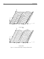
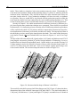
For example, let us compare the measured imperfections of two shells, the so-called
AS 2 from Caltech and KR1 from Technion. The first shell, AS 2 was measured by
Singer, Arbocz and Babcock in 1969 in the California Institute of Technology [4, 5]. The
second one, KR1 was measured by Abramovich, Ronith, Grunwald and Singer in 1977 in
Israel at the Technion Israel Institute of Technology [6]. Both shells were manufactured
by different people, in different places. The manufacturing process was the same. Plots of
the initial imperfections are reproduced in Figure 1.1. At first sight the imperfections of
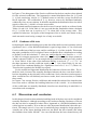
both shells look rather different. If one describes the imperfections using Fourier series,
as will be explained further in Chapter 4, for each of these shells a number of Fourier
coefficients can be calculated. In Figure 1.2 the circumferential variation of the halfwave cosine Fourier representation is plotted for both shells. Comparing both shells by
looking at the Fourier coefficients in this figure, it seems that the shells from Caltech have
been manufactured more accurately since the coefficients are smaller than those of the
Technion shell. The sizes of the Fourier coefficients corresponding to the circumferential
wave number where the axial half wave number k = 0 show a similar distribution, albeit
differing a factor of two.
The imperfection data of shells manufactured using the same fabrication process can
be used to create reliability functions. To do this a stochastic method like the Monte Carlo
Method or the First Order Second Moment method may be used. For a given reliability
an analytical knock-down factor λa can be determined [3]. This λa will replace γ, the
known very conservative knock-down value from NASA SP8007. The parameter λa will
be called an improved knock-down factor.
1.2 Why are imperfections important for the design of
shells?
The design of cylindrical shells involves participation of individuals from different segments of the engineering world. In the first place there will be a customer who is requesting a particular type of shell. Then the structural engineer will come up with a design,
3
4
Introduction
x
L
w/t
0.5L
3
2
1
θ = y/R
0
0
90
180
270
360
Caltech AS 2
x
L
w/t
0.5L
3
2
1
θ = y/R
0
0
90
180
270
360
Technion KR1
Figure 1.1: Measured initial shape of stringer stiffened shells
1.2 Why are imperfections important for the design of shells?
5
k
k
k
k
=
=
=
=
0
1
2
3
0.25
imperfection ξˆ =
q
2
A2kℓ + Bkℓ
0.3
0.2
0.15
0.1
0.05
0
0
5
10
15
20
25
circumferential wave number ℓ
Caltech AS 2
k
k
k
k
0.6
=
=
=
=
0
1
2
3
0.5
imperfection ξˆ =
q
2
A2kℓ + Bkℓ
0.7
0.4
0.3
0.2
0.1
0
0
5
10
15
20
25
circumferential wave number ℓ
Technion KR1
Figure 1.2: Circumferential variation of the half-wave cosine Fourier representation
6
Introduction
which in turn is built in the factory by the production people. The final product is returned
to the customer. This is the design process in a nutshell.
It is a well known fact that cylindrical shells are sensitive to imperfections, reducing
their load carrying capability substantially [7, 8, 9]. In the design process of a shell the
imperfections will not be known as the shell is still to be produced. Knowing the exact
imperfections of a shell would be the best solution for predicting the buckling load and
buckling mode of the shell. If one does not know the imperfections, assumptions will
have to be made. Of course after the shell has been built up, it should be verified if the
assumptions were acceptable. Measuring the imperfections of each shell takes time, and
money. Even more if the assumptions were optimistic and one should start all over.
To take into account the influence of these imperfections, it is common practice in industry to calculate the eigenmodes associated with the lowest eigenvalues of the shell [10].
If the imperfections in the structure resemble the eigenmodes or a combinations of these
modes, the reduction in the buckling load will be the largest [11]. To calculate the buckling behaviour of a shell where the imperfections are composed of a set of eigenmodes
corresponding to the lowest eigenvalues, is a relatively cheap operation compared to the
use of the real imperfections obtained using expensive testing. Furthermore, if the eigenmodes will be used as the assumed imperfection shape, it also needs to be decided what
magnitude to choose. On the other hand, if the imperfections do not resemble the eigenmodes, the calculated buckling load will be lower than the real one, yielding a conservative and therefore heavy design.
Suppose the imperfections could be related to production methods, to the quality of
the processes. Choosing a certain production process, the design engineer then knows
what the imperfections will look like. As an example one can think of an interstage of
a rocket. The interstage is built up of say 6 curved panels, jointed by offset lap splices.
Measuring the imperfections of this shell will definitely show the curved panels because
of the appearance of 6 circumferential waves.
1.3 Building an imperfection data bank
In the last decades a lot of imperfection measurements on thin-walled shells have been
performed. In the beginning of the 20th century only the buckling load and buckling
modes were measured in tests [12, 13, 14, 15, 16, 17]. The data is only available as
published papers containing tables with test data and photographs showing the buckled
shells. In the sixties Arbocz [18] started to measure the imperfections also. Along with the
published papers presenting the results, the data is also digitally stored. In the following
years, in several countries, researchers measured imperfections and buckling loads on
several types of shells [6, 19, 20, 21, 22, 23, 24, 25]. The first initiative to the data bank
was started in 1979 by Arbocz and Abramovich with the report ’The Initial Imperfection
Data Bank at the Delft University of Technology Part I’ [5], followed by Parts II - VI [23,
24, 26, 27, 28]. These reports contain the data of tests carried out at Caltech in the sixties
of the last century, and tests on ARIANE interstages produced by Fokker. There are
much more experimental data consisting of buckling load and imperfection data of shells
available, but these have been stored in many companies and universities in different
1.4 Layout of the thesis
countries. Thus, it is hard to get an overview of all data, or to have access to them. It
would be very convenient if all data would be accessible to all designers. Unfortunately,
this is not that easy because companies may have spent a lot of money on the tests, or data
might have restricted access because of security issues (defence technology!). After one
has succeeded in getting a set of test data, one will notice that different institutions use
different formats to store their data. Different units have been used: in Europe the SI units
are very common, in the United States many companies are still using Imperial Units.
In order to improve the knock-down factor in the lower bound formula for the buckling
load the influence of imperfections is subject of several research programs [2, 3, 18, 29,
30, 31]. This has lead to the following research questions:
• Is it possible to collect all available data of thin-walled shells and make them interactively accessible to shell designers and researchers?
• Can a relation be found between the imperfections and the manufacturing process
of a shell?
• Can statistical analysis using the tools of the interface of the imperfection data bank
help in the design of the shells?
To answer the first research question, published papers containing test results of shells
need to be collected. Next, datasets containing experimental data should be gathered
from all over the world. Next, the data needs to be digitized if needed and stored in a
computer system. An obvious choice for the latter is the creation of a data bank. It is
the primary purpose of this thesis to develop an imperfection data bank to store measured
imperfections to be made available to a world wide community of engineers. Along with
the data bank, tools to interrogate the data have been developed so that designers will be
more flexible in the design of new reliable shells similar to the ones included in the data
bank. Access to the data for shell designers and researchers working in different countries
can be made possible by connecting the data bank to the internet.
1.4 Layout of the thesis
One of the reasons that the stability of axially loaded thin-walled shells has been the
subject of research for so many years, is the large discrepancy between the theoretically
buckling load and the experimentally found value, both stored in the imperfection data
bank. A workaround of this problem was the introduction of the lowerbound [1]. The
traditional lower bound design philosophy is described in Chapter 2. Plots created by
the imperfection data bank are shown containing a lower bound curve and a collection
of experimental buckling data. In order to store the imperfection measurements in a data
bank, one has to first come up with measurement procedures that will accurately produce
the data desired. As part of this thesis a procedure was developed and imperfections have
been measured using different measurement equipment. The test equipment available at
the Faculty of Aerospace Engineering of the University of Technology Delft is described
in Chapter 3. This chapter starts with a short overview of the history of imperfection data
measurement. A generic test procedure for the imperfection measurement is described.
7
8
Introduction
Also the measuring of the new VEGA launcher vehicle currently under development by
ESA is described including the processing of the raw data. Once the imperfections are
measured, the data has to be presented to the users of the data bank in a convenient
amd meaningful fashion. Several ways to represent imperfections have been described
in Chapter 4. As an example the Fourier coefficients of the imperfection of the VEGA
interstage are determined. Subsequently these imperfection are compared with the ARIANE interstage data measured some years earliers. Analyzing all the available data, and
executing a test has made it clear which data needs to be stored in the data bank. This has
lead to the design of the data bank in Chapter 5. The design of the imperfection data bank
is described, starting with all its requirements. Also some technical background is given.
The usage of the interface is demonstrated by showing how to retrieve data from the data
bank of Arboczs favorite A-shell. This part of the chapter could be a good starting point
for an engineer who is interested in using the data bank. The final chapters deal with
the application of the imperfection data bank for statistical analysis. More precisely, the
statistical tools are discussed in Chapter 6. In Chapter 7 these tools have been used on
the research of the buckling behaviour of a shell with averaged imperfection. In the last
chapter some general conclusions and recommendations are presented.
Chapter 2
Lower Bound Design Philosophy
”I do not want to know, therefore I will not measure” [32]
In Chapter 1 the necessity of measuring the imperfections of thin-walled shells was discussed. Basically the lower bound theory is often used if there is no imperfection data
available, and one lacks time and/or money to obtain them. In this chapter the lower
bound theory will be explained. A difference is made between isotropic, orthotropic
and anisotropic shells. Isotropic shells have been manufactured from metal plates with
material properties which do not depend on the direction. Also these shells are not
stiffened with either rings or axial stiffeners. The orthotropic shells are similar to the
isotropic shells, however, rings or axial stiffeners or both are attached to the shell. Finally
anisotropic shells are composite materials assembled of a number of layers. The material
properties depend of the direction. A unified lower bound function will be derived which
makes it possible to combine all test data in one chart.
2.1 Design of shells using a hand book
If one looks at the design of thin-walled shells, the ones with a major imperfection sensitivity, structural engineers use buckling handbooks during the design process. Typically
these handbooks specify the use of the classical buckling formulas, and then multiply the
load by a so-called knock-down factor, to obtain the load a shell should be able to carry.
This method is an empirical approach based on historical test data. Measured buckling
load data are reported by normalizing them with predictions giving the knock-down factor
associated with imperfections, i.e. the fraction of the classical buckling load prediction.
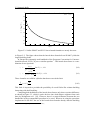
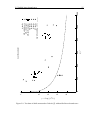
The experimental buckling loads are plotted with respect to the radius to thickness ratio
(R/t) in Figure 2.1. On the horizontal axis the shell-wall slenderness R/t is used since the
buckling stress of unstiffened shells increases linearly with t and decreases linearly with
R. On the vertical axis the normalized buckling load λ, which is defined as the ratio of
the experimental buckling load to the classical buckling load. The classical or theoretical
9
10
Lower Bound Design Philosophy
buckling load of a thin-walled cylindrical shell [33] is
where
E
2π t2
Pcl = σcl 2πR t = q
3(1 − ν 2 )
(2.1)
E
t
σcl = q
3(1 − ν 2 ) R
(2.2)
and E is the modulus of elasticity, and ν Poisson’s ratio. As can be noticed from Figure 2.1 the knock-down factor decreases with increasing R/t. The curved solid line in
the figure is the lower bound curve from which the knock-down factor is determined. It
provides a good lower bound for most of the test data [34]. The data in the plot show
a large scatter. If the buckling loads of the shells with R/t = 800 tested by Weingarten
et al. [35] can be considered to show a normal distribution, it will be possible that new
shells produced using the same manufacturing process will yield a normalized buckling
load lower than the lower bound value.
On the other hand, some test results are grouped at a large distance of the lower bound
curve. If one still uses the corresponding knock-down factor for these type of shells,
the structure would be very safe, and therefore much too heavy. For shells to be used
as rocket parts this is an argument to improve the knock-down factor. The question to
answer is why do these shells perform much better than others in the plot?
Several different analytical expressions including so-called knock-down factors to be
used in the design process of thin-walled shells are available. In the following part they
will be discussed for different types of shells, starting with isotropic shells, continuing
with stiffened isotropic shells and finally anisotropic shells.
2.2 Isotropic shells
The value calculated from the classical buckling load formula in the previous section is a
theoretical value in that sense that in real life a shell will collapse at a much lower load.
Sometimes the critical stress is calculated using
σc = 0.3E
t
R
(2.3)
which yields a buckling load of about 50% of the theoretical value as in Eq. (2.2) . The
50% is a knock-down factor on the theoretical load independent of the R/t ratio of the
shell. Kanemitsu and Nojima [38] proposed the following equation:
σc = 9 E
t
R
1.6
+ 0.16 E
t
L
1.2
t
R
1.2 (2.4)
This equation can also be written as
σc = 9 E
t
R
1.6
+ 0.16 E
R
L
1.2
(2.5)
λ = Pexp /Pcl
Figure 2.1: Test data for axially compressed isotropic shells
0
0.2
0.4
0.6
0.8
1
0
500
1000
R/t
1500
2000
2500
Arbocz & Babcock [5]
Ballerstedt & Wagner [14]
Crate, Lo & Schwartz [16]
Dancy & Jacobs [23]
Esslinger [36]
Harris, Suer, Skene & Benjamin [17]
Lundquist [13]
Robertson [12]
Weingarten, Seide & Morgan [35]
Lower bound, Eq. (2.7)
Lower bound plot
2.2 Isotropic shells
11
12
Lower Bound Design Philosophy
500
SP8007
Eq. (2.3)
Kanemitsu L/R = 2
Kanemitsu L/R = 1
Kanemitsu L/R = 1/2
450
400
σc [MPa]
350
300
250
200
150
100
50
0
500
1000
1500
2000
2500
R/t
Figure 2.2: Comparing different analytical knock-down functions
This allows the function can be plotted for different L/R ratio’s as shown in Figure 2.2.
The buckling stress depends on both t/R and R/L. Compared to Eq. (2.3) the knockdown factor for R/t < 300 is much higher, yielding a larger allowable load.
Although an update is being working on, the shell design handbook still used by
NASA is the well known SP-8007 report [1]. According to this report the buckling
stress for isotropic shells is calculated by
σc = γ σcl
(2.6)
where the knock-down factor γ is defined as
γ = 1 − 0.901(1 − e−φ )
(2.7)
and
1
φ=
16
s
R
t
To determine this formula, the test results were lumped without regard to production
manufacturing methods or the method of testing. The formula can be used up to a R/t
ratio of 1500. Further one should be careful using this formula if L/R exceeds 5, since no
experimental data of these types of shells were used to determine the empirical formula.
Notice further that in Eq. (2.6) the knock-down value γ was multiplied by the classical
buckling stress as shown in Eq. (2.2). The latter formula is valid for simply supported
boundary conditions. As the difference between rigorous solutions are obscured by the
effect of initial imperfections, this formula is used. Eqs. (2.3) and (2.6) are also plotted
2.2 Isotropic shells
13
1
ECCS
SP8007
0.9
λ = Pexp /Pcl
0.8
0.7
0.6
0.5
0.4
0.3
0.2
0
100
200
300
400
500
600
700
800
900
1000
R/t
Figure 2.3: NASA SP8007 and ECCS lower bound formulas are nearly the same
in Figure 2.2. The figure shows that the knock-down formula from SP-8007 yields the
largest buckling loads.
In Europe the commonly used handbook of the European Convention for Constructional Steelwork, ECCS [39] uses a similar equation 1 . This knock-down factor is a combination of two equations:
0.83
for R/t < 212
γ = q
1 + 0.01 Rt
0.70
γ = q
for R/t > 212
0.1 + 0.01 Rt
(2.8)
(2.9)
These formulas are valid for cylinders that do not exceed the limit
L
≤ 0.95
R
s
R
t
(2.10)
This limit is imposed to preclude the possibility of overall Euler-like column buckling
interacting with shell buckling.
Comparing both definitions of the knock-down factors only shows a minor difference
as shown in Figure 2.3, which is quite obvious since both factors originate from work
done by Weingarten et al. [34]. However, there is a major difference between the two
handbooks in the recommended procedure to be used. Whereas in using the procedure
implemented in SP-8007 the use of the knock-down formula already ends the buckling
1
ECCS is using the parameter α in stead of γ
14
Lower Bound Design Philosophy
t
t
w̄
w̄
lr
t
lr
lr
w̄
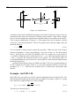
Figure 2.4: Imperfections
calculation, in the ECCS handbook the quality of the shell is taken into account. The imperfections of the shell are measured in a relatively crude manner. Using either a straight
rod or a circular template the imperfections should be checked everywhere on the surface.
This is shown schematically in Figure 2.4. The length of the rod or template is related
to the size of the potential buckles. The ECCS proposal states that the length of the rod
should be taken as
√
lr = 4 Rt
(2.11)
The rod should be held anywhere against the meridian. When the ratio of the largest
measured amplitude w̄ to the corresponding lr does not exceed 0.01, the knock-down
factor γ given in Eqs. (2.8) and (2.9) should be used. If lr equals to 0.02, the values of
γ are halved. When the ratio is in the interval 0.01 − 0.02, linear interpolation between
γ and γ/2 provides the knock-down factor to be applied. For values larger than 0.02
no recommendations are given, however it seems logical a shell with such imperfections
should be disposed of.
Another major difference between SP8007 and the ECCS is the recommendations of
ECCS of using an extra safety factor of 4/3 for axial compressed shells, on top of the
standard F.S. = 1.5. Thus one can conclude ECCS is much more conservative than
SP8007.
Example: shell IW1-20
Shell IW1-20 is one of the over 30 beer cans investigated by Dancy and Jacobs [23]. The
thin-walled shell manufactured from steel has a length of 100 [mm], a radius of 33 [mm]
and a thickness of approximately 0.1 [mm] yielding
1
R/t = 330. and φ =
16
s
R
= 1.13537
t
(2.12)
Then the lower bound value is
γ = 1 − 0.901(1 − e−φ ) = 0.3885
(2.13)
2.3 Orthotropic shells
15
x
z
d2
t
R
c2
ds
er
d1
c1
z
dr
es
t
R
y
Stringer stiffened
Ring stiffened
Figure 2.5: Orthotropic shell
The lower bound buckling load for this shell now becomes
Pγ = γ.Pcl = −3102.4 N
(2.14)
Comparing this to the experimentally found load
Pexp = −3890.0 N
(2.15)
one notices the lower bound value is conservative. Looking at all the buckling load data
of the beer cans of Dancy and Jacobs [23] as plotted in Figure 2.1 it can be seen that
these values show a large spread, where the minimum buckling load is positioned on the
lower bound curve. Therefore, for the beer cans there is no gain in spending energy in the
improvement of the lower bound curve.
It is interesting to mention that in the design of the beer cans other requirements exist which determine the wall thickness of the cans. In decreasing the wall thickness any
further the can might be damaged by sharp finger nails. On the other hand, can manufacturers are interested in the loading capability of shells where certain imperfections are
put on the shell surface on purpose. Think of, for example, embossed company logos.
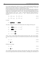
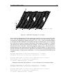
2.3 Orthotropic shells
Shells can be stiffened using axial stiffeners, rings or a combination of both. Let us consider a thin-walled cylindrical shell, reinforced by closely spaced circular rings attached
on the outside of the shell and with longitudinal stringers attached on the inside, as illustrated in Figure 2.5. If the stiffener spacing is small enough the stiffener effects are
smeared over the shell. Whether or not this yields satisfying results depends on the buckling mode. As a rule of thumb at least 5 stringers or rings should be situated on one half
16
Lower Bound Design Philosophy
wave of the buckling mode. If there are less, a discrete stiffener theory should be used
instead since the smeared stiffener wall assumptions become invalid [40]. For the latter
theory the shells will be referred to as stiffened isotropic shells.
For the smeared theory the cylinder is approximated by a fictitious sheet whose orthotropic
bending and extensional properties include those of the individual stiffening elements averaged out over representative widths or areas. The smeared bending stiffness per unit
width of the wall D̄x and D̄y in x− and y− direction respectively, and the smeared extensional stiffness’s of the wall E¯x and Ēy in x− and y− direction respectively are represented by
D̄x = D(1 + η01 ),
E¯x = C(1 + µ1 )
(2.16)
D̄y = D(1 + η02 ),
Ēy = C(1 + µ2 )
(2.17)
in which
Et3
D=
,
12(1 − ν 2 )
C=
Et
1 − ν2
The terms, which are a function of the dimensions of the stringers and rings, are:
EI01
and I01 = Is + As e2s
ds D
EI02
=
and I02 = Ir + Ar e2r
dr D
As
= (1 − ν 2 )
ds t
Ar
= (1 − ν 2 )
dr t
η01 =
(2.18)
η02
(2.19)
µ1
µ2
(2.20)
(2.21)
where ds and dr are the stringer and ring spacing respectively, and es and er the eccentricity of the stringer and the ring. The areas and the area moments of inertia of the stringers
are
As = c1 d1
Is =
1
c1 d31
12
(2.22)
(2.23)
Similarly for the rings:
Ar = c2 d2
Ir =
1
c2 d32
12
(2.24)
(2.25)
The contribution of the stringers and rings of the shell in the change of the critical buckling
load can be implemented in the knock-down formula by modifying the wall thickness of
2.3 Orthotropic shells
17
the shell. For orthotropic shells this lower bound formula is similar to the one for isotropic
shells:
γs = 1 − 0.901(1 − e−φs )
(2.26)
where
1
φs =
29.8
s
R
t∗
and
t∗ =
v
u
u
4 D̄x D̄y
t
E¯x Ēy
where the adjusted wall thickness t∗ is a function of the bending stiffness and the extensional stiffness of the stiffened shell. Whereas for isotropic shells the knock-down factor
was a function of R/t, for orthotropic shells it also depends on the number and size of
stiffeners which are implemented in the adjusted thickness t∗ .
The lower bound curve for the orthotropic shells is plotted together with experimental
data in Figure 2.6. On the vertical axis there is a difference noticeable when comparing it
to Figure 2.1. In Figure 2.6 ρ is the normalized load, where as a normalization term the
theoretical buckling load of a orthotropic shell is used. Thus
ρ=
Pexp
Pstf
(2.27)
where
Pstf = λm
Ckℓ Pcl
Here λm
Ckℓ is the critical (lowest) eigenvalue of the linearized stability equations using
membrane prebuckling [41]:
λm
Ckℓ
1
=
2
(
γ̄D,k,ℓ (γ̄Q,k,ℓ + αk2 )
+
αk2
αk2 γ̄H,k,ℓ
2)
(2.28)
where
γ̄D,k,ℓ =
D̄xx αk4
γ̄H,k,ℓ =
H̄xx αk4
+
D̄xy αk2 βℓ2
+
H̄xy αk2 βℓ2
+
D̄yy βℓ4
+
H̄yy βℓ4
,
αk2
=k
2 Rt
γ̄Q,k,ℓ = Q̄xx αk4 + Q̄xy αk2 βℓ2 + Q̄yy βℓ4 , βℓ2 = ℓ2
2c
π
L
Rt 1
2c R
2
(2.29)
2
and Pcl is the classical buckling load of a thin-walled cylindrical shell defined in Eq. (2.1).
The stiffness parameters and the wave number parameters have been defined in Appendix B. An interesting fact is the value of λm
Ckℓ for isotropic shells, since for those
m
shells λCkℓ = 1, yielding a normalized buckling load ρ = λ.
ρ = Pexp /(λm
Ckℓ Pcl )
Figure 2.6: Test data for axially compressed orthotropic shells
0
0.2
0.4
0.6
0.8
1
1.2
1.4
0
500
1000
R/t∗
1500
AB-shells [22]
AR-shells heavy [5]
AR-shells light [5]
AR-shells medium [5]
AS-shells [5]
KR-shells [22]
RO stringers [21]
Lower bound stiffened isotropic, Eq. (2.26)
Lower bound plot
2000
18
Lower Bound Design Philosophy
2.4 Anisotropic shells
19
Example: shell AS 2
Shell AS 2 is one of three stringer stiffened shells investigated by Arbocz and Babcock
[4, 5]. The aluminium 6061-T6 shell has a length of 139.7 [mm], a radius of 101.6 [mm]
and a wall thickness of 0.197 [mm]. Taken into account the properties of the 80 axial
stringers:
As = 0.7987 [mm2]
ds = 8.0239 [mm]
4
Is = 0.015038 [mm ] es = 0.3368 [mm]
(2.30)
using Poisson’s ratio ν = 0.3, the adjusted t∗ is calculated using Eqs. (2.16) - (2.26):
t∗ = 0.1091 [mm]
(2.31)
yielding a R/t∗ ratio of
R/t∗ = 931.5908
(2.32)
Notice this value for t∗ is smaller than the actual wall thickness because of the definition
shown in Eq. (2.26). In section 2.5 a different thickness will be introduced larger than
the actual wall thickness. This latter definition seems more convincing because of the
expected higher buckling load compared to an unstiffened shell having the same wall
thickness.
The lower bound value of the orthotropic shell is
γs = 1 − 0.901(1 − e−φs ) = 0.4238
(2.33)
using
φs =
1 q
R/t∗ = 1.02036
29.8
Although the value of t∗ is almost twice as low as the wall thickness t, the knock-down
factor is higher than for a shell without stiffeners using the same wall thickness, since φs
is used in stead of φ. The lower bound buckling load for this shell:
Pγ = γs .Pstf = γs . λm
Ckℓ Pcl = −1396.0 lbs
(2.34)
Comparing this to the experimentally found load
Pexp = −3211.7 lbs
(2.35)
one notices the lower bound value is very conservative. This again shows an update of the
knock-down parameters is needed.
20
Lower Bound Design Philosophy
middle surface
1
2
z0 z1
t/2
z2
zk−1
zk
k
N
layer number
z
zN −1
zN
t
L
Fibre orientation
{
Layers
1
Inner
2
Middle
θ
Outer
R
x
z
y
Figure 2.7: Geometry of composite material
Generatrix
2.4 Anisotropic shells
21
2.4 Anisotropic shells
Anisotropic shells are typically shells constructed out of several layers of a composite
material as shown in Figure 2.7. Each layer is a curved arrangement of unidirectional
fibers or woven fibers in a matrix. The fibers carry almost all the load whereas the function
of the matrix is to support and protect the fibers and to provide a means of distributing
load among and transmitting load between the fibers. The extensional stiffness terms Aij
and the bending stiffness Dij are defined as
Aij =
N
X
(Q̄ij )k (zk − zk−1 )
k=1
Bij =
N
1 X
2
(Q̄ij )k (zk2 − zk−1
)
2 k=1
Dij =
N
1 X
3
(Q̄ij )k (zk3 − zk−1
)
3 k=1
Q̄11
Q̄12
Q̄22
Q̄16
Q̄26
Q̄66
Q11 cos4 θ + 2(Q12 + 2Q66 ) sin2 θ cos2 θ + Q22 sin4 θ
(Q11 + Q22 − 4Q66 ) sin2 θ cos2 θ + Q12 (sin4 θ + cos4 θ)
Q11 sin4 θ + 2(Q12 + 2Q66 ) sin2 θ cos2 θ + Q22 cos4 θ
(Q11 − Q22 − 2Q66 ) sin θ cos3 θ + (Q12 − Q22 + 2Q66 ) sin3 θ cos θ
(Q11 − Q22 − 2Q66 ) sin3 θ cos θ + (Q12 − Q22 + 2Q66 ) sin θ cos3 θ
(Q11 + Q22 − 2Q12 − 2Q66 ) sin2 θ cos2 θ + Q66 (sin4 θ + cos4 θ) (2.37)
(2.36)
where
=
=
=
=
=
=
and the reduced stiffness
E1
1 − ν12 ν21
ν12 E2
ν21 E1
=
=
1 − ν12 ν21
1 − ν12 ν21
E2
=
1 − ν12 ν21
= G12
Q11 =
Q12
Q22
Q66
(2.38)
according to Jones [42]. Here E1 and E2 are the Young’s moduli in the 1 and 2 directions,
respectively, and νij is the Poisson’s ratio for transverse strain in the j-direction when
stressed in the i-direction. Further, G12 is the shear modulus in the 1 − 2 plane.
For anisotropic shells the lower bound formula is chosen similar to those of the
isotropic shells and orthotropic shells:
γa = 1 − 0.901(1 − e−φa )
(2.39)
where
1
φa =
29.8
s
R
t+
(2.40)
22
Lower Bound Design Philosophy
and
t+ =
s
4
D11 D22
A11 A22
(2.41)
and t+ is the adjusted wall thickness for anisotropic shells. Notice that in the formula for
t+ the extensional stiffness terms and the bending stiffness terms are used as before in the
definition of t∗ in Eq. (2.26).
The lower bound curve for the anisotropic shells is plotted in Figure 2.8 together with
experimental data. Similar to the plot with the experimental results for the orthotropic
shells, the value of R/t+ is used on the horizontal axis, where t+ is the adjusted thickness
of the shell, which includes the effect of the composite material. On the vertical axis one
can find the non-dimensional parameter ρ, the normalized load. As a normalization term
the theoretical buckling load of an anisotropic shell is used. Thus
ρ=
Pexp
Pani
(2.42)
where
Pani = λmnτ Pcl
Further λmnτ is the critical (lowest) eigenvalue of the linearized stability equations using
membrane prebuckling of the anisotropic shell [31]:
λmnτ
2
2
T̄3,m,n
T̄4,p,n
T̄1,m,n + T̄2,p,n + 2
+ 2
=
2 + α2
T̄5,m,n T̄6,p,n
2 αm
p
1
!
(2.43)
where
e
o
T̄1,m,n = γ̄D
∗ ,m,n − γ̄D ∗ ,m,n
e
o
T̄2,p,n = γ̄D
∗ ,p,n + γ̄D ∗ ,p,n
2
T̄3,m,n = γ̄Be ∗ ,m,n − γ̄Bo ∗ ,m,n + αm
T̄4,p,n = γ̄Be ∗ ,p,n + γ̄Bo ∗ ,p,n + αp2
T̄5,m,n = γ̄Ae ∗ ,m,n + γ̄Ao ∗ ,m,n
(2.44)
e
o
T̄6,p,n = γ̄A∗ ,p,n − γ̄A∗ ,p,n
e
The coefficients γ̄Ae ∗ ,m,n , γ̄Ao ∗ ,m,n , γ̄Ae ∗ ,p,n , γ̄Ao ∗ ,p,n, γ̄Be ∗ ,m,n , γ̄Bo ∗ ,m,n , γ̄Be ∗ ,p,n, γ̄Bo ∗ ,p,n, γ̄D
∗ ,m,n ,
o
e
o
γ̄D∗ ,m,n , γ̄D∗ ,p,n and γ̄D∗ ,p,n are functions of the stiffness parameters Aij , Bij and Dij .
2
and αp2 are functions of
Their definitions can be found in Appendix B. Both terms αm
the geometry of the shell and the number of waves of the buckling mode, also defined
in Appendix B. Notice that the eigenvalue λmnτ depends on the wave numbers m and n
and on Khot’s skewedness parameter τK [43]. This skewedness parameter is introduced
in order to account for the possibility of bending-twisting coupling.
Example: shell AW-CYL-1-1
Shell AW-CYL-1-1 is one of five layered, composite graphite-epoxy cylinders investigated by Waters [25]. The shell has a length of 14 [in], a radius of 7.99945 [in] and a
thickness of 0.039976 [in]. The shell has gotten 8 layers, lay-up [±45/0/90]s , each ply
ρ = Pexp /(λmnτ Pcl )
Figure 2.8: Test data for axially compressed anisotropic shells
0
0.2
0.4
0.6
0.8
1
1.2
0
500
+
R/t
1000
1500
Hühne [37]
Waters [25]
Lower bound anisotropic , Eq. (2.39)
Lower bound plot
2000
2.4 Anisotropic shells
23
24
Lower Bound Design Philosophy
has a thickness of 0.004997 [in]. Then the stiffness terms in Eq. (2.36) can be calculated
as
A11 = 0.326879.106
A22 = 0.326879.106
D11 = 39.8701
D22 = 31.3826
(2.45)
Taken into account these properties the adjusted t+ is calculated using Eq. (2.41) as:
t+ = 0.0104026 [in]
(2.46)
yielding a R/t+ ratio of
R/t+ = 768.9850
(2.47)
Then the lower bound value is
γa = 1 − 0.901(1 − e−φa ) = 0.35530
(2.48)
using
φa =
1 q
R/t+ = 0.93056
29.8
The lower bound buckling load for this shell:
Pγ = γa .Pani = γa .λmnτ Pcl = −14629 lbs
(2.49)
Comparing this to the experimentally found load
Pexp = −30164 lbs
(2.50)
Notice the lower bound value is very conservative for this shell. The lower bound for the
other 4 shells in the group with R/t+ about 400 is also conservative, however not a lot of
weight can be saved on these shell if the bound is improved, Figure 2.8.
2.5 Unified lower bound curve
In the NASA report SP8007 [1] the functions for the lower bound curves for isotropic
and orthotropic shells are not the same. The lower bound curve for the isotropic shell is
a function of R/t, whereas for the orthotropic shell it is a function of R/t∗ , where t∗ has
been defined as:
t∗ =
v
u
u
4 D̄x D̄y
t
E¯x Ēy
(2.51)
This definition has a disadvantage. If the stringer and ring areas of the shell are very
small, and the shell can be considered to act as an isotropic shell, the parameters η01 , η02 ,
µ1 and µ2 defined in Eqs. (2.18)-(2.21) will go to zero. The stiffness terms simplify to
D̄x ⇒ D
2.5 Unified lower bound curve
25
D̄y ⇒ D
E¯x ⇒ C
Ēy ⇒ C
Substituting this result into Eq. (2.51) yields a thickness
t
t∗ = √
12
(2.52)
Using this formula for t∗ in the lower bound formula of the orthotropic shell should yield
the equation of the isotropic shell, therefore in Eq. (2.26) a coefficient 1/29.8 in the expression for φs is used in stead of 1/16 in φ in Eq. (2.7).
Although the definition of t∗ in Eq. (2.51) is an elegant formula, it is reasonable that in
the limit where the stiffeners are negligibly small, the adjusted thickness is
t∗ = t
In stead of the definition in Eq. (2.51) it is suggested to multiply this formula by
yielding
tu =
√
12 t∗ =
√
v
u
u
4 D̄x D̄y
12 t
√
12
(2.53)
E¯x Ēy
which can be rewritten using Eqs. (2.16) and (2.17) to
tu =
v
u
u
(1 + η01 ) + (1 + η02 )
4
t
(1 + µ1 ) + (1 + µ2 )
t
(2.54)
A benefit is that the lower bound formula Eq. (2.7) can also be used for the stiffened shell.
Similar to the stiffened shell, for anisotropic shells another definition for t+ as an
alternative to Eq. (2.41) will be used. Let
u
t =
√
+
12 t =
√
12
s
4
D11 D22
A11 A22
(2.55)
√
which is in fact equal to the definition as used in Eq. (2.41) multiplied by 12. For a
single layer of isotropic material with material properties E and ν and thickness t the
stiffness terms are
Q̄11 = Q11
Q̄22 = Q22
and
Q11 = Q22 =
E
1 − ν2
(2.56)
26
Lower Bound Design Philosophy
then
Et
1 − ν2
Et
= Q22 (z1 − z0 ) = Q22 (t/2 − (−t/2)) =
1 − ν2
A11 = Q11 (z1 − z0 ) = Q11 (t/2 − (−t/2)) =
A22
Et3
12(1 − ν 2 )
Et3
= 1/3 Q22 (z13 − z03 ) = 1/3 Q22 (t/2)3 − (−t/2)3 =
12(1 − ν 2 )
D11 = 1/3 Q11 (z13 − z03 ) = 1/3 Q11 (t/2)3 − (−t/2)3 =
D22
Substituting these equations into the formula for the adjusted wall thickness, Eq. (2.55):
tu = t
(2.57)
Also for the anisotropic shells the lower bound formula Eq. (2.7) can be used in the design
of a new shell.
Recall shell AS 2 in the example on page 19 where the wall thickness t∗ is almost half
the actual wall thickness. Calculation of the unified thickness yields
√
(2.58)
t = 12 × 0.1091 = 0.3779 [mm]
which is about twice the value of the wall thickness of the wall. This result seems more
appropriate.
In the following examples the unified lower bound theorem can be used to generate
one plot containing the experimental results of shells where the walls consists of isotropic
material, possibly stiffened with axial stringers and/or rings, and walls built up using a set
of anisotropic layers.
Example: comparison of stiffened and unstiffened shells
The shells reported in [5] can now be plotted in a single lower bound plot, which makes
it easier to compare different types of shells. The shells in the report are the results of
imperfection surveys carried out at Caltech in the sixties of the last century. The shells
consist of a set of copper electroplated shells (A-shells), nickel electroplated shells (Nshells), machined brass shells (B-shells), welded stainless steel shells (ST-shells), stringer
stiffened aluminium shells (AS-shells), and finally ring stiffened aluminium shells (ARshells). The results are plotted in Figure 2.9. Notice on the vertical axis the in the normalm
ization the factor λm
u has been used. For orthotropic shells this will be replaced by λCkℓ ,
for anisotropic shells by λmnτ .
The first thing which can be observed is the clustering of the data. The shells within a set,
which have about the same R/t ratio, show a small spread of the buckling load. This is
important as this makes it realistic to move the lower bound line upwards.
However, the ST-shells all collapsed before the load associated with the lower bound
curve was reached. These shells were reported to have shown plastic buckling [5]. The
0
0.2
0.4
0.6
0.8
1
1.2
0
200
400
ρ = Pexp /(λm
u Pcl )
Figure 2.9: Test data of shells measured at Caltech [5] with unified lower bound curve
u
R/t
600
Lower bound plot
800
1000
A-shells
AR-shells heavy
AR-shells light
AR-shells medium
AS-shells
B-shells
N-shells
ST-shells
Lower bound, Eq. (2.7)
1200
2.5 Unified lower bound curve
27
28
Lower Bound Design Philosophy
shells were cut from commercial, longitudinal welded, type 304 stainless steel tubing.
As the fabrication process cannot be compared with the carefully procedure as followed
for the other shells, and the buckling behaviour is completely different, they will not be
discussed any further.
The buckling loads in Figure 2.9 are all normalized. Recall that for isotropic shells
the normalization factor
λm
Ckℓ = 1.0
The normalized buckling load for the isotropic unstiffened shells is lower than for the stiffened orthotropic shells. The normalization factor λm
Ckℓ is calculated for a stiffened shell
with simply supported SS-3 boundary condition but the ends of the shells are clamped
during the test, approaching CC-4. Because of this clamped boundary condition the calculated buckling load will be lower than should be expected, yielding a conservative result [40].
Notice the buckling load of the isotropic A-shells, B-shells and N-shells seems to be independent of the R/t ratio, despite of the definition of the knock-down factor. No real
conclusion can be drawn because of the small number of tests within these sets.
2.6 Discussions and conclusion
In this chapter lower bound plots have been shown for isotropic shells, orthotropic shells
and anisotropic shells. The lower bound curves plotted in these figures are empirical
equations used as a knock-down value to determine a safe buckling load of a shell design.
Notice that the plots are similar: the empirical functions for the lower bound curves of
the isotropic shells, orthotropic shells and anisotropic shells are the same if the stiffness
parameters valid for isotropic shells are substituted in each of the three equations (2.7),
(2.26) and (2.39).
The lower bound curves originate from the NASA report SP-8007 [1] and are based
on experimental data dated before 1968. More recent data have been plotted into these
figures. These newer shells manufactured using newer production techniques will be designed much more conservative than shells designed many years ago, because the lower
bound curve has not been adjusted for modern technology where the quality and repeatability have been improved. Using the ECCS handbook [39], which is also based on the
experimental data used for SP-8007, is even more conservative since an extra safety factor
is recommended for axial compressed shells. Substantial weight savings can be achieved
if the lower bound theory is improved, which is possible if the effect of modern technology is used in the theory.
The lower bound formula for isotropic shells is used up to a R/t ratio of 2500. Notice
that the formula which can be used up to 1500 according to SP-8007 also yields smaller
buckling loads for the higher R/t values as shown in Figure 2.1!
The experimental buckling loads found for the beer cans show a large spread. Since
the lowest buckling load is found on the lower bound curve, there is no profit in spending
energy in the improvement of the lower bound curve for these cans.
2.6 Discussions and conclusion
The normalized buckling loads of some shells are higher than 1.0 in the lower bound
plot for the orthotropic shells in Figure 2.6. Because the buckling loads are normalized
using the theoretical buckling load of a orthotropic shell with simply supported boundary
conditions, this can be expected for shells tested with clamped boundary conditions.
One should stay compatible with the lower bound curves defined in SP-8007 [1], a
handbook of which the curves have been the basis for newer hand books as well. Therefore the lower bound curve for the anisotropic shells has been based on the curve for the
orthotropic shells. At the end of this chapter a unified lower bound curve has been proposed which has the advantage that all data can be plotted in one figure. Furthermore, in
this new approach the adjusted thickness will be equal to the real thickness in the limit
case where the areas of the stringers and rings go to zero.
29
30
Lower Bound Design Philosophy
Chapter 3
Imperfection Measurement Procedures
There are only a couple of plants in the world producing beer cans in the
amount of millions each day. To be more precise, the machine which starts off
with a small cup, pushing this cup through 3 or 4 rings spits out around 1000
cans each minute. Our beer can is not a unique species, however, it is unique in
that sense that a set of 30 was tested 25 years ago in the Faculty of Aerospace
Engineering at Delft University of Technology by Dancy and Jacobs [23].
The normalized buckling loads of the circular cylindrical shells shown in the lower bound
plots in Chapter 2, Figures 2.1, 2.6 and 2.8, have been measured using different measurement equipment. This chapter starts with some historical background, followed by
a general description of the test procedure. After the description of the test equipment
available at the Faculty of Aerospace Engineering of the University of Technology Delft,
the measurement of the VEGA interstage is described. This measurement served several
purposes. New imperfection data of a thin-walled shell manufactured using state of the
art techniques can be added to the imperfection data bank, furthermore the test acted as
an experience for the author in the process of setting up the test equipment, installing the
shell, performing the test, meanwhile solving unexpected problems.
3.1 The history of imperfection measurements
Researchers started to measure the imperfections of thin-walled cylinders in the 1960s. It
was then when Arbocz [44] built his well-known AS-2 shell, measured the imperfections
and loaded the shell up to the point where it collapsed. Koiter [7] proved initial imperfections play a large role in the buckling behaviour of shells. In his calculations he assumed a
geometric imperfection shape and determined that it could significantly reduce the buckling load of the shell. Many years before Koiter and Arbocz, engineers and researchers
were already interested in thin-walled shells. The theoretical buckling formula derived
by Timoshenko [33] is one of the early expressions used in predicting the buckling load
of shells. Robertson [12], Esslinger [36], Weingarten [34] and many others manufactured
their own shells and loaded them until failure. These tests were somewhat unsatisfactory
in the sense that the theoretical buckling load as predicted by Timoshenko was hardly ever
reached. One could say that this was partly caused by the fact that production techniques
31
32
Imperfection Measurement Procedures
were not as advanced as they are today, so near perfect shells could not be manufactured,
also the test facilities may not have been 100% perfect either, but still this could not explain the sometimes dramatic difference between theory and experiment. Being practical,
engineers started using the so-called knock-down factor. Empirically derived, this is the
factor which will be multiplied by the theoretical calculated buckling load to get the lower
bound load below which most of the shells will not fail.
3.2 Available shells
To measure imperfections first of all one needs shells. These shells are available at different locations in different shapes depending on the type of application that they are used
for. One can distinguish between three different categories of shells. First at a research institute or university shells might be manufactured for the single purpose of research. The
produced shells are measured inside out: every aspect is noted. The load carrying capability before failure or buckling is determined or the natural frequency of the shells. The
collapse load will be predicted analytically, possibly by using advanced FEM programs,
and verified by the real experiment. If a large number of shells is tested, the reliability of
the shells can be established.
Secondly, a company develops a new cylinder, maybe a conical interstage between
two stages of a rocket. Before launching it a number of test shells will be measured. First
the weight of the structure is measured and the exact location of the centre of gravity.
Next the imperfections and finally the collapse load will be determined experimentally.
Third, and last, this same company will produce parts of a rocket which is to be
launched. Researchers might get an opportunity to measure the imperfections before the
rocket is used to take one or more satellites into orbit. Obviously the collapse load for
these last sets of shells will not be available, although it might be possible to measure the
maximum loads during lift-off.
Full scale shells are very interesting, but are also the least available. This is not just a
money problem, it is also more practical to test smaller shells. The test of a large number
of small shells can be performed relatively fast, does not need to cost a lot of money, and
can still provide valuable information on the behaviour of the shells manufactured by a
certain production method. As an example a set of small beverage cans, similar to the one
shown in Figure 3.1 will be described in the section 3.4.1. Measurements on a full scale
model of the VEGA are discussed in section 3.5.
3.3 Test procedure
The description of the test procedure is schematically shown in Figure 3.2. After the
production phase, the measuring of the shell can start. The shell will be mounted in its
fixture. If possible the ends of the shell are connected to stiff end rings, which will be part
of the structure in its final setup. Without these rings the stiffness of the shell is rather
low and the shell would definitely change its shape slightly when it is moved from one
location to another. As the behaviour of the shell is strongly influenced by the shape and
magnitude of the imperfections mounting of these stiff end rings is recommended. For
3.3 Test procedure
33
Figure 3.1: An old version of a beer can
laboratory shells, different boundary condition configurations may exist. They will be
discussed when the test equipment is described.
When the imperfections are measured the data needs to be checked: the data might
contain flaws which will need to be corrected. The flaws might be introduced because
of a variety of reasons. For example the sensor measuring the imperfections might have
jumped over a rivet, or maybe over a small cut in the shell. This will cause a small nonexisting peak in the imperfection. Missing or incorrect data will either be interpolated
using the neighbouring data points or substituted by so-called ’magic numbers’. These
numbers will be discussed in the description of the program BESTFIT in section 4.2.
This program is the next step in the test procedure. The base shape of the cylinder does
not need to be the same as the best-fitted cylinder. A manufacturer starts by manufacturing
a shell of radius say 1.5 [m]. The manufacturing technique causes the shell not to be
exactly round or perfect. The difference between the manufactured shell, and the desired
shell of radius 1.5 [m] depends on the fabrication method. This difference can be seen as
the manufacturing signature of a certain fabrication method. In this thesis the difference
between the manufactured shell and a perfectly cylindrical shell is called the imperfection
of the shell. The best-fit shell is found by minimizing the imperfections using a least
square method. This best-fit shell can have a mean radius of say 1.49 [m] and even have
a small conicity as well. Details are discussed in the next chapter.
The imperfections could be stored as such, and as a matter of fact, they are stored in
the database as a datafile, but a more elegant way of describing them is the use of Fourier
coefficients, because analytical tools like MIUTAM [45] and ANILISA [46], which calculate the buckling load, assume sine and cosine series for the deformation of a shell, and
can use the Fourier coefficients in their calculations immediately.
The Fourier coefficients will show the dominant mode of the imperfection of a cylin-
34
Imperfection Measurement Procedures
company
production
university
x,y,z
test data
or
i,j,w
measurement
fix data, remove errors
transfer data into
standard format
bestfit
corrected test data
raw data
w w.r.t. reference shell
w w.r.t. perfect shell
Databank
find Fourier coefficients
Fourier coefficients
check imperfection field
recompute field
compare with bestfitted data
measure buckling load
LAUNCH !
Figure 3.2: Overview of test procedure
3.4 Measuring tools
der, and provide an easy method of comparing different shells to each other. Different
representations of the imperfection using these Fourier coefficients are described in Chapter 4.
The measured data always needs to be checked. As already mentioned one should
correct flaws. The way to find out about errors in the data is by plotting the imperfection
field. Any irregularities should be explained.
Standardization of the data is an important issue. This is one of the objectives of the
imperfection data bank project. There are as many data formats as there are engineers.
It is not just the usage of either millimeters or inches, although very expensive losses of
rockets have been the result of mixing up those different units. Also data can be stored
in hundreds of different formats. The geometry is stored as either [mm] or [inch] in the
database. One could of course argue on the usage of just SI-units, however, a lot of
experimental data is available in either [mm] or [inch], and if a manufacturer is using
dimensions like radius of 4 [in], and length of 8 [in] of a shell, the corresponding SI
dimension are not really nice.
The final step in the test procedure depends on the purpose of the particular shell. The
laboratory shells and full scale test shells will be loaded until failure, providing a value
for the collapse load and the failure mode. The shells which will be part of a real rocket
will be launched. In theory the encountered stresses during the flight could be measured
yielding the stress distribution in the shell.
When all the data have been measured, checked, and possibly corrected, they will
be entered into the data bank. The right to enter data should be restricted. To ensure
the contents of the data bank will remain of a high quality, and no errors or deletion of
data will occur, only certified people should be authorized to update the data bank. More
information is found in the user manual in Appendix A.
After the data is entered into the data bank it will be available to all authorized structural engineers. The next section deals with different test equipment used for measuring.
3.4 Measuring tools
Several methods have been and are still used to measure the imperfections of cylindrical
shells. Either the radial distance with respect to a reference perfect shell is used, or the
data just contain a set of x,y,z coordinates. At the Faculty of Aerospace Engineering
of Delft University of Technology, three testing machines have been built, capable of
measuring cylindrical and/or conical shells of different sizes. They are listed in Table 3.1.
3.4.1 Stonivoks
STONIVOKS is an acronym for ’Statistisch ONderzoek naar de invloed van Initiële VOrmonzuiverheden op de Kniklast van Schaalconstructies’ (Statistical research into the influence of initial deformations on the buckling load of shells). The primary objectives
of the test apparatus Stonivoks [47] is it should be able to measure the imperfections of
35
36
Imperfection Measurement Procedures
Testing machine Size of shells
Stonivoks
small cylindrical shells
radius 33 [mm], length 100 [mm]
Univimp
medium scale cylinders
radius of 120, 180, and 240 [mm],
length respectively 240, 360, and 480 [mm]
Amivas
large cylindrical or conical shells, like ARIANE II or VEGA
radius 1..2 [m], length 1..3 [m]
Table 3.1: Imperfection measurement devices at the TU Delft
a small cylindrical shell. This has to be possible in both unloaded and loaded state. A
photograph of a small cylindrical shell in the test apparatus is shown in Figure 3.3.
Figure 3.3: Stonivoks
The choice of the shells to be measured during the development of Stonivoks was
determined by the maximum allowable size of Stonivoks itself. As it should be capable
of measuring the deformation of the shell under loading, the test apparatus should fit in
the compression machine, also developed at the Faculty of Aerospace Engineering of the
Technical University in Delft. Small cylinders normally used as beer cans happened to be
the best choice instead of, for instance, electro-plated shells like shell A-8 described in
Chapter 5.4. The latter have the advantage that they can be of any shape, any wall thickness, but for larger number of shells they take too much time to produce. The beer cans
3.4 Measuring tools
37
all have the same shape but do have small imperfections. They do not display isotropic
material behaviour and have wall thickness that is not constant, both due to the production
process. The compressive collapse load is measured, and finally the post failure buckling
pattern has to be measured.
Special attention is given to the fact that the measurement device should not influence
the behaviour of the shell. Details can be found in reference [47], however, one interesting item will be discussed here. If the shell is loaded in axial direction it is possible to
measure the displacements perpendicular to the shell surface. This is used to show how
the shell deforms before buckling occurs. During the measurement the shell is rotated.
The shell is free to rotate in the test apparatus, however, as there will always be some
friction in the bearings, a torsional moment can be introduced in the shell, yielding shear
forces. These shear forces combined with the axial stress would have a significant effect
on the behaviour of the shells. In Stonivoks one of the end disks has a so-called core
width a membrane at the end as shown in Figure 3.4 as part number 18. This membrane
is provided with a castellated rib, part number 19, at its outer edge. The membrane is
mounted to the bottom end disk. The polar moment of inertia of the core with inner and
outer radius of r1 = 15 [mm] and r2 = 22 [mm] respectively is calculated as:
π 4
Ip =
r2 − r14 = 288450 [mm4 ]
(3.1)
2
and the polar moment of inertia of the thin-walled shell with radius of 33 [mm] and a
thickness of 1 [mm]:
Ip = 2π r 3 t = 22580 [mm4 ]
(3.2)
Therefore the torsional stiffness of the core is over 12 times as large as of the shell. This
means only a small part of the torsional moment which is used to overcome the friction
in the bearings (part numbers 14 and 15 in Figure 3.4 ) is carried by the shell. The effect
on the buckling behaviour is negligible.
The measurement procedure is fully automatic. Once installed the test will be controlled by a computer which is triggered by small switches. The lower disk (part number
22 in Figure 3.4) has at its outer rim 100 evenly spaced narrow slits. Installation of a small
lamp and a photo-cell triggers the AD converter to measure 100 data points in circumferential direction.
The boundary conditions of the specimen need special attention. The cylinders are
inserted in the circular channels in the end disks, which will be filled with ’Cerrobend’.
This ’Cerrobend’ is a metal like material with a low melting temperature. When solidified,
the boundary conditions of the cylinder can be considered clamped. Also the membrane
connecting the core to the lower end plate is mounted using ’Cerrobend’.
The imperfections of the shell are measured using a linear voltage displacement transducer (LVDT). This transducer makes contact with the shell, and therefore applies a load,
very small though, perpendicular to the shell surface. The deformations caused by this
small load are negligible. Other options using non contact probes like eddy current or capacitive sensors have a disadvantage of having a relatively large sensor or coil diameter.
For an imperfection range of 2 [mm], a sensor diameter of at least 8 [mm] is necessary.
The measured value will be an average of the value under the sensor, therefore imperfections with small wave lengths will be ’flattened’ out when the area used for measuring is
38
Imperfection Measurement Procedures
Figure 3.4: Sectioned view showing the mechanism of Stonivoks [47]
3.4 Measuring tools
too large. Optical measurements using laser are complicated and too expensive, at least
when Stonivoks was first built.
When the imperfections are measured in circumferential direction, the pick-up will
also move in axial direction at the same time, as the pick-up is mounted on a support
which is moved up or down by means of a screw spindle. The vertical and rotational
movement are coupled such that one revolution of the specimen corresponds to a vertical
displacement of the pick-up of 1 [mm]. This results in imperfections on a helix on the
shell surface. One will need a small program to calculate the imperfection pattern on a
regular mesh of axial and circumferential scans.
3.4.2 Univimp
UNIVIMP is an acronym for ’UNIverseel instrument voor het bepalen van initiële IMPerfecties van schaalconstructies’ (Universal instrument for the survey of initial imperfections of thin-walled shells). Univimp is an enlarged version of Stonivoks. The principal
setup of the apparatus is rather similar to Stonivoks, although there are some differences.
The initial structural design of Univimp was done by prof.ir. W.D. Verduyn [47].
Univimp, shown in Figure 3.5, is designed for cylinders with a diameter of 240, 360,
and 480 [mm] and a height of respectively 240, 360, and 480 [mm]. Other diameters
can be accommodated for, but need some additional structural components like end rings,
core, and membrane springs. It can measure the initial imperfections at zero axial compressive load and also the development of the imperfections under increasing compressive
load. The instrument can be adapted to the 800 kN compression testing machine of the
Faculty of Aerospace Engineering of the Technical University in Delft. Further it can
measure the nonlinear vibration behaviour of thin-walled cylindrical shells under changing axial load conditions.
Univimp consists of a rotating platform mounted on the base plate of the apparatus,
and a column on which a carriage is going up and down and to which the imperfection
measurement transducer is mounted. The column is not perfectly straight, therefore before the test it is calibrated using an accurately machined reference beam. Unlike Stonivoks the movement of the carriage is not mechanically coupled to the rotation of the
shell. Therefore the measured data are supplied per circumferential scan. Per scan 200
data points are read. The axial displacement of the carriage is controlled by the user, its
minimum step size is 0.1 [mm].
The shell is put in two circular end disks. In those disks a circular channel provides space for the shell. As for Stonivoks described in section 3.4.1 the channel will
be filled with Cerrobend. The end disk is mounted on the rotating platform which in turn
is mounted to the bottom of the apparatus, via a pair of axial and radial bearings. To
remove any possible movement in the axial bearing, they are loaded by means of disk
springs. One cannot avoid the fact that the centroid of the shell is not at the same location
of the rotation centre of the platform. To remove the resulting rigid body motion, also the
displacement of the end-rings is measured.
The whole instrument can be controlled by hand or by computer. Full documentation
is found in the literature [48]. In 1989 Mertens used Univimp for the measurement of the
buckling behaviour of three different sets of aluminium shells [49].
39
40
Imperfection Measurement Procedures
Figure 3.5: Univimp
3.4.3 Amivas
AMIVAS is an acronym for ’Automatisch Meetsysteem voor het bepalen van de Initiële
imperfecties VAn Schaalconstructies’ (Initial imperfection survey instrumentation for thinwalled shells). This device, shown in Figure 3.6, is much larger than Stonivoks and Univimp. Because of its size it is not one apparatus but a set of parts which when combined
can perform the same function as the other test machines, except for measuring deformation during loading of the shell. This is not possible and is mainly caused by the fact that
the Faculty of Aerospace at Delft University of Technology does not possess a compression machine big enough to test the size of shells Amivas can measure.
Amivas consists of three units:
• Rotation platform
3.4 Measuring tools
Figure 3.6: Amivas test equipment used for VEGA interstage
• Column
• Electronic equipment
Each of the units exists of multiple parts which need to be assembled at the test location.
It has been practice to drive to the location where the shell was built, and perform the
measurement on site. The shells which can be measured with Amivas can have diameters
up to 4 meters, which are rather difficult to transport. Also as the shell producers do not
stand in line when it comes to facilitating researchers the possibilities of imperfection
measurements of full scale rocket parts it was decided to make the Amivas a portable
device. The setup is sketched in Figure 3.7.
The rotation platform consists of two wooden rings, both built up of four segments.
Between the two rings ball bearings are placed. The lower ring is fixed to the platform, the
upper ring carries the shell. The rotation of the shell is controlled by a set of rollers. Two
fixed rollers are placed on the outside of the shell, on the inside two spring-loaded rollers
are mounted. When the shell is rotated, the springs will keep the rollers on the shell lower
ring. The shell will therefore only rotate, the translation of the shell in the horizontal
plane during rotation will be small, however not negligible. The motion of the shell is
determined by the shape of the ring and the rollers. To measure this rigid body motion
a diametrically running steel beam is attached to the lower wooden ring. In the middle
of the beam a support for four displacement transducers is placed. Four transducers are
placed in two pairs, with the centre lines of the pairs perpendicular to each other.
The reference ring is mounted to a steel frame which is attached to the upper wooden
41
42
Imperfection Measurement Procedures
LVDT
adjustable column
LVDT
shell
LVDT
LVDT
wooden rings
reference ring
LVDT
roller
Figure 3.7: Amivas test setup
3.5 VEGA - Europe’s small launcher
ring. The reference ring, its frame, the wooden ring and the shell are one rigid body. The
combination of the reference ring and the four transducers makes it possible to measure
the translations of the shell. As also the reference ring is not perfectly round, this ring was
calibrated. Using the data of the four transducers the rigid body motions are subtracted
from the shell imperfection measurements.
The adjustable column is a large, over 4 meter long, bar, on which a carriage is attached. It is connected to a heavy frame. The columns position is vertical for cylindrical
shells, and it can be tilted to measure cones. The column has been calibrated. The carriage is pulled upward by an electric motor. The scans will be in axial direction starting
from the top to the bottom of the shell. The measuring device is a LVDT mounted on the
carriage. During the measuring of the axial scan, the system will trigger every 10 [mm].
The final unit is the control unit of the engine, and the equipment necessary to read
the LVDT data, convert the analog to digital data and the computer to store all the data.
3.5 VEGA - Europe’s small launcher
In September 2005 the opportunity arose to do some measurements on the very first full
scale model of the interstage 1/2 of the VEGA rocket. VEGA, shown in Figure 3.8 is currently developed as a co-operative project within the ESA framework. It will complement
the performance range offered by the ARIANE family of launchers with a capability for
smaller payloads. Dutch Space has designed interstage 1/2 of the VEGA. The conical
shell has a length of 2138 [mm], the diameter of the bottom ring is 3035.5 [mm]. The
cone angle of the shell is 14.2◦ . It is built up of two parts bolted together. The lower part
consists of 8 segments, the upper part with the smaller radius of just 4 segments.
In the design phase the engineers took some imperfections into account, however these
were assumptions. As the value and pattern of the imperfections play an important role
in the stability of the shell, they were anxious to know what the real imperfections looked
like. An important question was: ’have we been too optimistic, or too conservative’. A
yes answer to the first question costs a lot of money, and to the second imposes weight
penalty.
The equipment to use, Amivas, was used for measurements on the ARIANE II some
years ago. A number of modifications needed to be done. As computers become ancient
in months, not years, the data acquisition needed an update. New wooden rings on which
the interstage needed to be positioned were produced. As devices for actually measuring
the imperfection LVDTs are used. They are very accurate, but do need to make contact
with the specimen. For the VEGA interstage 1/2 this is not a big problem, as the wall
thickness of 6.3 [mm] prevents the LVDTs to cause any extra imperfections.
3.5.1 Test setup
The interstage is placed on a set of two rings which can rotate relative to each other
enabling the shell to turn. Each ring is built up of four segments yielding a ring where the
width of the segment is 350 [mm] and the inner radius 1500 [mm]. As the shell is heavy a
large number of roller bearings (216 in total) were mounted. To minimize the friction of
43
44
Imperfection Measurement Procedures
Figure 3.8: VEGA and its interstage 1/2 ( courtesy of Dutch Space )
the bearings on the wooden rings, a thin Trespa plate was glued to the upper ring. Part of
the lower wooden ring with the roller bearings clearly visible is shown in Figure 3.9.
The shell is placed on the wooden disks carefully, trying to centre it. As no special
equipment is used an offset of say 1 or 2 [mm] is normal. On the end ring of the shell
two sets of rollers, each set consisting of an inside and an outside roller guide the shell
when it is rotated as shown in Figure 3.10. The location of the rollers was already shown
in Figure 3.7 in Chapter 3.
The fabrication process almost guarantees a perfectly circular shape of the end ring.
After casting the ring, it is put in a lathe. Finally at 254 spots the ring is milled to make
room for the bolts which are needed to connect the interstage to the first stage of the
VEGA. The bottom ring should be an almost perfect ring.
A column with the measuring devices, i.e. LVDTs, is connected to a tripod. Two
LVDTs measure the displacement of the end rings and one LVDT moves up and down
over the test specimen as shown in the pictures assembled in Figure 3.11.
Because of the many holes in the interstage, the measurement is only automated partly,
As the LVDT needs to be lifted manually in the neighborhood of a hole. During the
measurement the tripod will not move. After measuring the first axial scan, the shell
is rotated over a small angle, typical around 2 degrees. When the shell is rotated one
cannot avoid that the shell will also translate slightly because of some play in the system.
Although this translation will be small, it will be of the same order of magnitude as the
measured data. In the original test setup during the ARIANE measurements a reference
ring with four displacement transducers was used as discussed in section 3.4.3. During
3.5 VEGA - Europe’s small launcher
45
roller bearing
Figure 3.9: Wooden support ring with roller bearings
the VEGA measurement this ring was not installed. This saved some time during the test
setup, however, as will be shown later more analytical work compared to the ARIANE
measurement was needed to correct the measured data. In the next section it is shown how
the induced displacement of the shell during rotation which is caused by the test setup,
can be eliminated using the measured data of the LVDTs placed on the end rings.
The complete test setup with the VEGA interstage 1/2 in position is shown in Figure 3.12.
3.5.2 Phantom imperfections and play in the test setup
In the measurements of the ARIANE shells [50], an almost perfect aluminium disk was
placed in the middle of the top wooden disk, and fixed to this disk. The aluminium
disk was calibrated. When the shell was rotated, and so the top wooden disk, also this
’perfect’ disk rotated. There were four LVDTs placed on the border of the disk. The
imperfection data of the shell were corrected for the translation measured by these LVDTs
on the calibrated disk. If we assume that the bottom end ring is without imperfections, the
aluminium disk is not really needed. An advantage is a less complex test setup. Next it
will be shown that because the VEGA test lacks the calibrated disk, the shell imperfections
will have to be corrected by looking at the behaviour of the end ring rotating under control
of the rollers.
An impression of the irregularities of the lower end ring is shown in Figure 3.13.
Actually the line shows the data measured by the LVDT on the lower end ring shown in
46
Imperfection Measurement Procedures
Figure 3.10: Rollers guide the interstage
Fig. 3.11. Clearly noticeable are four circumferential full waves, and some small waves
added to it. As the end ring is precisely machined the small waves cannot be part of the
imperfection and should be removed from the measured data. The small waves are caused
by a small translation of the shell in the horizontal plane because of the play in the system
and show up in the measured imperfection data.
The correction of the measured data therefore involves two steps, i.e. the play in the
test setup and the effect of the rollers. In order to correct the measured end ring data, they
will be represented by means of a Fourier series using full waves, i.e.
w̄(θ) = t
N
X
(Aℓ cos ℓθ + Bℓ sin ℓθ)
(3.3)
ℓ=1
Because the lower part of the VEGA interstage 1/2 is built up using eight segments, it
is expected that in the imperfection plot of the end rings eight full waves will show up.
Therefore it is assumed that all wave numbers of nine and higher can be considered as
small waves originating from the translations of the shell during rotation. Indeed if one
looks at Figure 3.14 it can be seen that if one selects eight full circumferential waves as
the separator between long and short waves, the short waves produce a small part of the
total imperfection as compared to the long waves. The Fourier coefficients responsible for
the small waves, i.e. A9 , A10 , ... and B9 , B10 , ... are substituted into Eq. (3.3). The result
is the equation for the play in the test setup and will be subtracted from the measured data
of the shell first.
The effect of the rollers on the imperfection will be looked at next. As the lower end
ring will be in constant contact with the roller, this will introduce an error which needs
to be adjusted for. Let a local imperfection w̄A exist in the ring at roller A, and w̄B at
roller B as is seen in Figure 3.15. Because of this imperfection the centre of the shell
will move to another location, yielding a displacement measured by the LVDT at point C.
This means that if an imperfection exist in the ring, it will show up in the measured data
when the point passes the LVDT, and it will also appear in the data when it passes roller
A and roller B. The latter displacements will be called phantom imperfections.
Let the imperfection at point C be defined by
w̄C = ξ sin mθ
(3.4)
3.5 VEGA - Europe’s small launcher
47
Figure 3.11: LVDTs on shell and lower end ring
then the imperfection at roller A can be written as
w̄A = ξ sin m(θ + αA )
and the imperfection at roller B
w̄B = ξ sin m(θ − αB )
where αA and αB are the angles between OA and OC and between OB and OC respectively. For a perfect ring the angles αA and αB are equal to each other:
αA = αB = α
(3.5)
As the changes in αA and αB caused by the imperfections are only small, these angles are
assumed to be constant. The value of angle α for the VEGA test setup is
α = 42.5◦
(3.6)
Looking at Figure 3.15 it can be observed that
a2 + h2 = (R + w̄A )2
b2 + h2 = (R + w̄B )2
(3.7)
(3.8)
The distance between the two rollers A and B is constant and depends on the measurement
setup
δAB = a + b
(3.9)
48
Imperfection Measurement Procedures
Figure 3.12: Test setup of the VEGA interstage 1/2 imperfection measurement
and
a=
2
(R + w̄A )2 − (R + w̄B )2 + δAB
2δAB
(3.10)
Notice the imperfection w̄ is positive outward.
Next the angles αA and αB are calculated using
sin αA =
a
b
and sin αB =
R + w̄A
R + w̄b
(3.11)
The imperfection at point C is retrieved from the measured data from the LVDT yielding:
w̄C = −wLVDT + (h − horig )
(3.12)
where h can be solved from Eq. (3.7) and the original height using the equation:
horig =
v
u
u
tR 2
δAB
−
2
!2
(3.13)
Because of the guiding of the lower end ring of the shell by the rollers, the measured data
of the ring will be different from the imperfection shape. This effect is only showing as
a resizing of the imperfections. The number of circumferential wave numbers as shown
in the measured data is not changed, meaning if there are four full waves in the imperfections, the measured data will also show four waves, but the magnitude will be different.
3.5 VEGA - Europe’s small launcher
49
1.5
measured data
1
w̄C , [mm]
0.5
0
-0.5
-1
-1.5
0
20
40
60
80
100
120
140
160
180
200
scan number
Figure 3.13: Measured data of end ring
Also no extra waves appear in the data. If one calculates the magnification of the waves
due to the roller mounting for each wave separately, it is observed that some wave numbers are amplified whereas others are reduced. In Table 3.2 the magnification factors for
the global imperfections are shown for all the larger wave numbers. Notice further the
table starts with m = 2, as the m = 1 term is caused by the offset between the centre
of the shell and the rotation point of the test setup. This offset will be eliminated in the
best-fit step in the next section.
wave number magnification factor
2
-0.88179
3
-1.8257
4
-2.3357
5
-2.1439
6
-1.3510
7
-0.37371
8
0.27454
Table 3.2: Magnification factor of the Fourier coefficients of the end ring imperfections
Applying the scale factors on the Fourier coefficients of the measured data yields the
actual imperfection on the end ring. The results of the calculations are shown in Figure 3.16. The continuous line are the points measured by the LVDT, whereas the dashed
line is the actual imperfection of the end ring. The small waves due to the play of the
setup have been subtracted from the original measured data, and the long waves have
50
Imperfection Measurement Procedures
1.5
mode up to 8 full waves
measured data
w, [mm]
1
0.5
0
−0.5
−1
−1.5
0
20
40
60
80
100
120
140
160
180
200
180
200
scan number
Fourier coefficients of up to 8 circumferential waves
1.5
mode 9 and more waves
measured data
w, [mm]
1
0.5
0
−0.5
−1
−1.5
0
20
40
60
80
100
120
140
160
scan number
Fourier coefficients of 9 and more circumferential waves
Figure 3.14: Separation of the ring imperfection
3.5 VEGA - Europe’s small launcher
51
θ
O
R
w̄ B
+
+
w̄
A
R
h horig
αA
A
αB
B
C
LVDT
a
b
δAB
Figure 3.15: Phantom imperfections
been rescaled according to Table 3.2. Notice in this figure the measured data have been
multiplied by (−1) because of the different sign compared to the imperfection. Comparing the imperfections to the measured data one can see that the imperfections are smaller:
the set of rollers increase the magnitude of the data.
The size of each wave number given by the value of the Fourier coefficients is printed
in Table 3.3, where the most significant Fourier coefficients have been highlighted. As
expected the ovalisation term A2 is one of them. Furthermore coefficient B4 for four
full circumferential waves is also expected as the upper part of the VEGA interstage 1/2
consists of four segments. Finally a peculiar mode of seven full waves, expressed by the
term B7 is highlighted. This mode might be explained because at one side of the interstage
two large holes are positioned above each other.
As the wall thickness of the shell is 6.3 [mm], from Figure 3.16 one can see that the
imperfections of the ring are smaller than 10 % of the wall thickness.
In the determination of the Fourier coefficients it is assumed that all measured points
are equidistant. Some axial scans were measured at a small offset to avoid the LVDT pass
a number of rivets. This will only have a small effect on the small circumferential waves
and therefore do not cause a problem in the analysis of the ring imperfection where only
the large waves up to eight are used.
The corrections of the measured data for the end rings, consisting of a contribution of
the phantom imperfections and the play in the test setup have been subtracted from the
measured data, yielding the imperfection pattern of the end ring. As the end ring is rigidly
connected to the interstage, also the interstage will experience the same displacements,
therefore the correction on the end ring need to be made on the interstage as well. The
52
Imperfection Measurement Procedures
1.5
measured data
imperfection
w, [mm]
1
0.5
0
-0.5
-1
-1.5
0
20
40
60
80
100
120
140
160
180
200
scan number
Figure 3.16: Imperfections of the end ring
ℓ=
t Aℓ
t Bℓ
1
0.041434
-0.019722
2
0.18667
0.022204
3
0.091176
-0.034813
4
-0.024564
0.28124
5
-0.014070
0.053697
6
-0.051933
0.071078
7
0.040636
0.16560
8
0.022484
0.086654
Table 3.3: Fourier coefficients of the VEGA interstage 1/2 lower end ring
results are shown in Figure 3.17. It should be noted that the amount of analytical work
could have been reduced a lot if the reference ring with four displacement transducers
was installed during the test of the shell.
3.6 Discussions and conclusion
The general procedure of measuring the geometric imperfections of cylindrical or conical
shells has been described. Details have been provided for the three measuring devices
available at the Faculty of Aerospace Engineering of the Technical University in Delft,
i.e. Stonivoks, Univimp and Amivas.
It is recommended to mount stiff end rings at both ends of the shell to increase its
stiffness. Without these rings the stiffness of the shell is rather low and will therefore
change its shape slightly when it is moved from the location where the imperfections
were measured to the pressure testing machine. This would result into different measured
values for the imperfections because of the ovalisation of the shell. The end rings will
prevent this. Incorrect or missing imperfection data are interpolated using the information of neighbouring points. If this is not possible, the data are replaced by so-called
’magic numbers’. Those are large numbers recognized by programs such as for instance
3.6 Discussions and conclusion
53
x
L
w/t
0.5L
3
2
1
θ = y/R
0
0
90
180
270
360
Figure 3.17: VEGA interstage 1/2 raw data
BESTFIT to identify missing data. The BESTFIT program calculates the imperfections
with respect to a perfect shell, using a least square method.
Measurements were performed on the VEGA interstage 1/2. The test setup used was
a simplification of the test on an interstage of the ARIANE some years earlier. This
simplification introduced so-called phantom imperfections caused by the guiding of the
set of rollers. A new technique was developed to eliminate these imperfections from the
measured data.
The work on the VEGA interstage showed that when the opportunity arises, one
should measure as much as possible. The data bank as will be discussed in Chapter 5
has to contain the edited data such as the best-fitted imperfections, as well as all raw
data. The latter should be included in the data bank to be able to process them when new
techniques become available.
54
Imperfection Measurement Procedures
Chapter 4
Analyzing the Test Data
”How many boulders are lying on the moorlands of Drente,
probably pushed and pulled by prehistoric man for many years,
half a meter each day ... Many years he has been busy, day in,
day out, during the night he was sleeping next to his stone.”,
Beyond sleep [51]
After a set of shells has been built and its imperfections have been measured, the shells
were loaded until they collapsed. Next the measured data, both buckling loads and imperfection data can be stored into the data bank. Before doing so, the data will be analyzed
carefully. Possible errors need to be corrected, furthermore additional data related to the
shell geometry will be calculated. In this chapter an overview of this process will be given
and the necessary computer programs will be discussed.
4.1 Some background
In Chapter 2 the importance of knowing about the imperfections of a thin-walled shell has
been described. The calculation of the buckling behaviour is suggested to be performed
using a hierarchical approach [3]. This approach consists of three levels of analysis sophistication. As a first level analysis simple programs may be used to investigate the
behaviour of perfect shells [31, 52]. The deformation in both axial and circumferential
direction is described using goniometric functions. In these Level-1 codes membrane
prebuckling is used. This is followed by more advanced analytical programs where the
deformation in circumferential direction is still described using goniometric functions,
but in axial direction the deformation is solved from the differential equations. In Level2 the boundary conditions and the effect of prebuckling deformations are solved rigorously [46]. Finally, as the highest fidelity analysis, the problem is solved using a Finite
Element Program like ABAQUS [53], STAGS [54] or NASTRAN [55]. An important
aspect is the inclusion of effects of geometric imperfections on the buckling of a shell.
In the Level-2 codes it is possible to take the real imperfections into account, however
because of the simplicity of the codes normally only a few terms, that is a few Fourier
coefficients can be used. When a Level-3 code is used, the number of terms depend on
the mesh refinement of the model. As a rule of thumb for proper convergence five mesh
55
56
Analyzing the Test Data
points per half-wave of the characteristic buckling displacement should be used.
4.2 Best-fit of the shell
If a shell is mounted on the test equipment, a certain amount of misalignment cannot be
avoided as is shown in Figure 4.1 for a cylinder and a cone. The centre of the rotating
platform will probably not match precisely with the centre of the shell. Furthermore the
rotating axes of the platform will not be exactly parallel to the centre axes of the shell.
Notice the sketches are exaggerated: one will try to keep the offset (X1 , Y1) of the shell
reference axes X ′ Y ′ Z ′ to the axes of the test apparatus XY Z as small as possible. Also
the angles between Z ′ and X and Y given by ε1 and ε2 respectively, will be set very
small. The transducers measure the irregularities of the shell surface. The measured data
should be corrected for the small misalignment of the shell. This is done by the program
BESTFIT [56]. It calculates the best-fit shell by using the method of least squares. Adding
the squares of all distances, including the misalignment parameters X1 , Y1 , ε1 , ε2 , radius
R and cone angle αc , all defined in Figure 4.1, yields:
S=
N
X
d2i =
i=1
N
X
i=1
(Ri − R)2 = f (X1 , Y1 , ε1, ε2 , αc , R)
(4.1)
Minimizing S with respect to the unknown parameters X1 , Y1 , ε1 , ε2 , R and αc , yields
six nonlinear algebraic equations in six unknowns. The first four terms, i.e. X1 , Y1 , ε1
Z
Z′
Z
Z′
R
L
R1
αc
L
ε1
ε2
X1
Y
R2
Y′
X X′
X′
Y
Y′
X
Y1
Figure 4.1: Best-fit cylinder and cone reference axis
and ε2 tell us how the shell is installed in the test apparatus. They do not tell anything
on the quality of the shell. The latter two: radius R and cone angle αc show the global
deviation of the product compared to the ’perfect’ shell. The program BESTFIT will
4.3 Fourier coefficients
57
calculate the imperfections with respect to the perfect shell, where this perfect shell does
not necessarily need to have the dimensions planned by the producer of the shell. Of
course the changes in R and αc are likely to be small. An extended solution of the bestfitting of conical shells is found in the thesis work of Sebek [50].
4.3 Fourier coefficients
The imperfection field of a thin-walled shell can be described using different methods.
The easiest way is just use the imperfection data itself. The data can be plotted showing
the irregularities with respect to a perfect shell. The data can be exported and used as input
for a finite element code, giving the engineer the opportunity to calculate the collapse
load of this shell using the true imperfection data instead of an assumption such as a set
of eigenmodes.
It is also possible to find a polynomial function which fits through all the measured
data points. Having found such a polynomial yields the opportunity to find values of
imperfection data in points not directly measured. This can be useful if for a finite element calculation the chosen mesh uses different and possibly more points than measured.
This should be done with care since the interpolated points in between might not be as
expected.
Much more information can be distilled from the imperfection data if they are described using a Fourier representation of the field. Since the Fourier representations use
sine and cosine functions the imperfections will be compiled of a set of waves in axial
and circumferential direction. Because buckling modes are also described as a number
of waves in both directions, and furthermore in analytical tools like MIUTAM [45] and
ANILISA [46], sine and cosine series are used to assume the deformation of a shell, it
is a natural choice to use Fourier coefficients. The 2-dimensional Fourier coefficients describing the imperfection surface can be obtained by a double harmonic analysis. Several
representations have been used. They will be mentioned in the next section, followed by
the selection of which one will be preferred. All Fourier coefficients are calculated by the
code HARMONIC [56].
Researchers have been using the imperfections from the data bank, implementing the
imperfections using Karhunen-Loève expansion instead of Fourier coefficients [57, 58].
This is an efficient way to investigate shell buckling due to random geometrical imperfections, however, this representation is not used in the Level-2 MIUTAM [45] and ANILISA [46] codes mentioned above.
4.3.1 Half-wave cosine representation
The half-wave cosine representation involves two sets of harmonic components Akℓ and
Bkℓ . The imperfection will be written as:
w̄(x, θ) = t
M
X
i=0
Ai0 cos
M X
N
X
iπx
kπx
+t
cos
(Akℓ cos ℓθ + Bkℓ sin ℓθ)
L
L
k=0 ℓ=1
(4.2)
58
Analyzing the Test Data
where x is the axial coordinate, x = 0 .. L and θ the circumferential angle, θ = 0 .. 2π.
Note that for cylindrical shells L is equal to the height of the shell whereas for conical
shells L is the slant shell length and H the height of the cone, Figure 4.1. Notice that
the representation uses half-waves in axial direction, but full waves in circumferential
direction. The first term using Ai0 is the so-called axisymmetric imperfection term since
it is independent of the circumferential angle. All Fourier coefficients are dimensionless,
therefore multiplication with the wall-thickness t will yield the value in [mm] or [in],
depending on the unit of t.
4.3.2 Half-wave sine representation
The half-wave sine representation uses sine waves in axial direction of the shell instead
of cosine waves.
M X
N
M
X
X
kπx
iπx
+t
sin
(Ckℓ cos ℓθ + Dkℓ sin ℓθ) (4.3)
Ci0 sin
w̄(x, θ) = t
L
L
i=1
k=1 ℓ=1
The selection of this representation cannot satisfy the boundary irregularities as the sine
will always yield zero on the boundaries. This may sound like a definite no to this representation, but it is still used quite frequently. Analytical tools used for solving the buckling problems are less complicated if one uses sine functions as assumed buckling modes.
Furthermore, the imperfections at the boundaries will be very small as different parts of
cylindrical shells or cones need to be connected to each other. Finally, the imperfection
measurements do not include points exactly on the boundaries. Therefore using sine instead of cosine representation is not going to make a lot of difference to the calculated
results of the numerical analysis of the shells.
4.3.3 Full-wave representation
Furthermore, the full-wave representation, involving the determination of four sets of
harmonic components:
w̄(x, θ) = t
+ t
N X
N
X
k=0 ℓ=0
N
N X
X
cos
2kπx
(Akℓ cos ℓθ + Bkℓ sin ℓθ)
L
sin
2kπx
(Ckℓ cos ℓθ + Dkℓ sin ℓθ)
L
k=1 ℓ=0
(4.4)
can represent the boundaries exactly, but one will need Akℓ , Bkℓ , Ckℓ and Dkℓ . The total
number of coefficients will be the same, but there does not seem to be an advantage over
using half-wave cosine.
4.3.4 Alternate method
And the fourth representation, called the alternate method which is actually a combination
of the first and second, i.e. the half-wave cosine and half-wave sine representation:
w̄(x, θ) = t
M
X
i=0
Ai0 cos
M X
N
X
iπx
kπx
+t
sin
(Ckℓ cos ℓθ + Dkℓ sin ℓθ)
L
L
k=1 ℓ=1
(4.5)
4.3 Fourier coefficients
59
This method was introduced to make use of the convenient analytical solutions using
half wave sine functions, and adding a correction term for the boundary irregularity which
is axi-symmetric.
4.3.5 Preferred method
There are no real pros and cons for each method. The preferred choice of the author is,
however, the use of half-wave cosine, as the representation of the boundaries are much
better than using half-wave sine representation. Using full wave representation would
do the job as well, but has not been frequently used in the literature, and does not have
any advantages over half-wave cosine. Also it is using Akℓ , Bkℓ , Ckℓ and Dkℓ , therefore
using half-wave cosine with only Akℓ and Bkℓ is more elegant. The alternate method is
not preferred since it performs somewhat worse than half-wave cosine because the extra
term with respect to the half-wave sine representation only corrects the boundaries axisymmetrically.
The effect of some of the Fourier coefficients has been made visible in Figure 4.2.
A01 , B01
excentricity
A00
radius
A02 , B02
ovalisation
A03 , B03
radius
Figure 4.2: Fourier coefficients linked to modes
The coefficient A00 in the half-wave cosine representation associated with
iπx
0πx
= cos
= 1.
L
L
is a constant term, independent of the axial position or of the circumferential angle. It
implies a correction on the radius of the best-fit shell. This coefficient should be very
small, preferably 0.0, since the best-fit routine BESTFIT of the previous section should
have eliminated this. An eccentricity of the shell is visible as a non zero value of the
Fourier coefficients A01 and B01 . These coefficients will be practically zero since the
eccentricity was removed by program BESTFIT when determining the offset distance
(X1 , Y1). The coefficient A02 associated with
cos
cos ℓθ = cos 2θ
is the ovalness of the shell. If the boundaries of the shell are unstiffened and if the shell
is not stiff in the circumferential direction then by just having the shell lie on its side is
60
Analyzing the Test Data
the easiest way to deform in ovalisation. The right most picture in Figure 4.2 shows the
effect of A03 .
Other terms identify certain aspects of a shell. For example, looking at the measurements performed on ARIANE shells in the eighties, they show large values of A08 and
A28 , both highlighted in bold-faced text in Table 4.1.
Akℓ
ℓ=
k=0
k=1
k=2
k=3
k=4
k=5
k=6
k=7
0
1
2
-0.00866 0.00036 -0.16224
0.00761 -0.00152 -0.05315
0.25009 0.01847 0.03652
-0.02831 0.02012 0.00275
0.04806 0.01735 0.01696
-0.00741 -0.01123 -0.01207
0.03304 0.00139 0.00851
-0.01784 -0.00406 0.01093
3
-0.09161
-0.00540
0.03498
0.06336
-0.00004
-0.01835
0.00000
0.01065
4
0.07086
0.01930
-0.00424
-0.03235
-0.02750
0.03022
-0.00631
-0.01205
5
-0.03132
0.03725
-0.01499
-0.01510
0.01192
-0.02655
0.00994
0.01006
6
7
8
-0.05259 0.00952 0.58020
-0.04139 0.01537 -0.03440
0.02586 0.00492 -0.19456
0.01008 -0.02479 -0.06445
0.01737 0.00266 -0.11414
-0.00755 0.00285 0.06890
-0.00825 0.00741 -0.06405
0.00844 -0.00381 -0.01548
Bkℓ
ℓ=
k=0
k=1
k=2
k=3
k=4
k=5
k=6
k=7
0
0.00000
0.00000
0.00000
0.00000
0.00000
0.00000
0.00000
0.00000
1
0.00471
0.00311
-0.02869
0.00402
-0.00197
0.02314
-0.00555
-0.01486
2
0.03685
0.08659
0.01962
0.03446
0.00193
0.00484
0.00706
0.01897
3
4
5
6
7
8
0.07711 0.07469 0.08175 -0.03577 0.02601 -0.10489
-0.00259 0.00348 0.01652 0.03490 -0.08445 -0.06000
-0.03047 -0.05438 -0.02521 0.04595 -0.02149 0.02041
0.04404 0.00868 -0.04009 -0.01451 0.03591 0.02009
-0.00358 -0.01457 -0.02786 -0.00439 0.02434 0.01541
-0.01355 0.00170 0.04330 0.00306 -0.00474 -0.00215
0.00502 -0.01279 0.00003 0.00266 0.00353 0.02331
0.02070 0.00271 -0.02790 -0.00128 0.00831 0.00582
Table 4.1: Fourier coefficients ARIANE II interstage 2-3, half wave cosine
Fourier representation
What does it mean? Looking at the production of this shell, the shell is built up of eight
curved panel segments, these eight segments are connected to each others longitudinal
edges or seams. This cannot be done without influencing the overall geometry of the
shell and is also the reason shell manufacturers do not like the term imperfections that
much. They prefer the term manufacturing signature. This will be discussed in more detail in Chapter 5.4. Figure 4.3 shows the plot of the imperfection of this shell, where the
influence of the eight segments are clearly visible.
4.4 Check validity of data
The Fourier coefficients of all four representations discussed in the previous section are
calculated using the program HARMONIC. One of the input files of this program is the
best-fitted imperfection field from program BESTFIT. Do the coefficients represent the
imperfection correctly? For example, if only the largest coefficients are taken into account, the dominant modes of the imperfection field will show, however, the smaller
4.4 Check validity of data
61
x
L
w/t
0.5L
3
2
1
θ = y/R
0
0
90
180
270
360
Figure 4.3: ARIANE II interstage 2-3, raw data
waves will have disappeared. For this purpose two routines have been written, RECOMPUTE [56] and DELTACHECK [56]. RECOMPUTE will, as its name already suggests,
recompute the imperfection pattern using Eqs. (4.2) - (4.5). If the recomputed pattern
as calculated by RECOMPUTE corresponds with the best-fitted shape, one can assume
the coefficients are correct. Because comparing a large number of numbers is a difficult
(and boring) task, DELTACHECK has been written. It will subtract the two imperfection data sets from each other. The result should be equal to zero. This mode can be
plotted using the same plotting tool as for BESTFIT and RECOMPUTE. Apart from the
plot DELTACHECK yields a numeric indication of the differences beween best-fitted and
recomputed shape. If only Fourier coefficients > 0.01 were selected DELTACHECK will
compute:
Average amplitude of absolute differences : 0.00295
Standard deviation of absolute differences : 0.00277
Average amplitude of actual shell imperfections: 0.02325
Percentage ratio of absolute differences
to actual imperfections: 12.68227
Setting the truncation limit smaller to > 0.001 will improve the recomputed shape:
Average amplitude of absolute differences : 0.00085
Standard deviation of absolute differences : 0.00100
Average amplitude of actual shell imperfections: 0.02325
Percentage ratio of absolute differences
to actual imperfections: 3.66458
62
Analyzing the Test Data
at the cost of many more Fourier coefficients. In Figure 4.4 the results of the verification are plotted. The plot at the top shows the best-fitted shell, the plots at the left
are the recomputed fields and on the right the difference between the recomputed and the
best-fitted data.
Notice that one needs to recalculate the half-wave cosine coefficients to verify the A’s
and B’s, and recalculate the half-wave sine coefficients to verify the C’s and D’s. As previously mentioned, using the half-wave sine representation one cannot get the boundary
conditions correct. Therefore, the DELTACHECK output will show non zero values at
the boundaries.
Once the Fourier coefficients have been obtained, it is also possible to recompute the
imperfection field yielding an approximate shape at any point of the shell, not just on
the measured grid. This is useful when one likes to use the imperfections in a Finite
Element calculation where the nodal points lie on a mesh which differs from the mesh of
the measured data points.
4.4.1 Best-fit of VEGA
Although the shell and the measuring equipment are carefully positioned, it cannot be
avoided that the centre of the shell does not precisely coincide with the rotation centre of
the test setup, or that the beam with the LVDTs for the shell imperfection measurement
might not be exactly parallel to the shell surface. The BESTFIT program as was described
in section 4.2 will remove these small offsets. The resulting plot of the imperfection of
the VEGA interstage is shown in Figure 4.5.
In Table 4.2 the Fourier coefficients of the half-wave cosine Fourier representation
are listed. The bold numbers show the larger value of the Fourier coefficients associated
with two, four and eight circumferential full waves. Two full waves correspond to the
ovalness of the shell. The interstage is made up of two parts. The lower part is assembled
using eight curved panels whereas the upper part consists of four curved panels. As
it turns out both four and eight full waves are visible in the imperfection pattern. The
value of these large coefficients does not exceed 5% of the wall thickness, which is a
significant improvement over the values measured some years ago on the ARIANE II
rockets where the largest coefficients were almost 60% of the wall thickness as can be
seen from Table 4.1.
4.5 Discussions and conclusion
In this chapter it has been shown how the test results are interpreted. A brief introduction was given to the hierarchical approach as a way to solve buckling problems [3].
After the unavoidable misalignment of the shell in the test fixtures has been removed
using the program BESTFIT, the geometric imperfections are described using Fourier
series using program HARMONIC. The accuracy of the coefficients is checked by the
programs RECOMPUTE and DELTACHECK. Programs HARMONIC, RECOMPUTE
and DELTACHECK will be on the requirements list of the interface to the imperfection
data bank. It is shown that using half wave cosine representation the imperfections are
4.5 Discussions and conclusion
63
x
L
0.5L
w/t
3
2
1
θ =y/R
0
0
90
180
270
360
best-fit of shell IW1-20
x
x
L
L
0.5L
0.5L
w/t
w/t
3
3
2
2
1
1
θ =y/R
0
0
90
180
270
θ =y/R
0
360
0
90
180
recomputed field
half-wave cosine representation
x
270
360
deltacheck
x
L
L
0.5L
0.5L
w/t
w/t
3
3
2
2
1
1
θ =y/R
0
0
90
180
270
360
θ =y/R
0
0
90
recomputed field
half-wave sine representation
180
270
360
deltacheck
Figure 4.4: Shell IW1-20: check on validity of the Fourier coefficients
64
Analyzing the Test Data
x
L
w/t
0.5L
3
2
1
θ = y/R
0
0
90
180
270
360
Figure 4.5: VEGA interstage 1/2 best-fitted data
described in the most accurate way. The value of the Fourier coefficients indicate some
features of the shell. The ovalness of a shell represented by the coefficient A02 is also a
measure of overall stiffness of the shell. If a shell is stiffened using a set of axial stiffeners
or circumferential rings this is also seen by looking at these coefficients. The values of the
Fourier coefficients, and which of them are the most important ones is part of the manufacturing signature of a production process. This signature also includes information
relating to the material used, and the production equipment.
4.5 Discussions and conclusion
65
Akℓ
ℓ=
0
1
2
3
4
5
6
k = 0 -0.00196 -0.00143 0.00473 0.01564 0.01081 0.00830 0.01354
k = 1 0.00163 -0.00121 0.02045 0.01412 -0.00702 0.00266 -0.00962
k = 2 0.00032 -0.00042 0.00445 -0.00805 -0.00937 -0.00922 -0.00964
k = 3 0.00664 -0.00289 0.01460 -0.00374 -0.01272 -0.00309 0.00678
k = 4 0.00103 -0.00554 0.00391 -0.00371 -0.00327 -0.00164 0.00182
k = 5 0.00086 -0.00558 0.00342 -0.00239 0.00102 -0.00001 0.00118
k = 6 -0.00025 -0.00241 0.00220 -0.00185 0.00071 0.00135 0.00001
k = 7 -0.00200 -0.00124 0.00102 0.00044 0.00175 0.00029 -0.00139
7
-0.00213
0.00088
-0.00362
-0.00180
0.00038
0.00112
-0.00063
-0.00003
8
-0.01027
-0.00192
0.01930
-0.00206
-0.00782
-0.00047
-0.00156
0.00359
Bkℓ
ℓ=
k=0
k=1
k=2
k=3
k=4
k=5
k=6
k=7
0
0.00000
0.00000
0.00000
0.00000
0.00000
0.00000
0.00000
0.00000
1
-0.00169
-0.00155
0.01407
-0.00107
0.00440
-0.00020
-0.00183
-0.00105
2
0.03927
0.02493
-0.01969
-0.00853
-0.00731
-0.00205
-0.00129
-0.00048
3
4
5
6
7
8
0.01109 -0.04635 0.00150 0.00000 -0.01578 -0.03105
0.01346 0.01359 0.00511 -0.00309 0.00493 0.01968
-0.00525 0.01491 0.00605 -0.00415 -0.00333 -0.00162
-0.00469 0.00140 0.00481 0.00062 0.00160 -0.01143
-0.00484 0.00188 0.00009 -0.00096 -0.00058 0.00110
-0.00385 0.00148 -0.00045 0.00324 0.00071 0.00165
-0.00156 0.00067 -0.00063 0.00291 -0.00069 0.00191
-0.00249 -0.00122 -0.00111 0.00045 -0.00012 -0.00126
Table 4.2: Fourier coefficients VEGA interstage 1/2, half wave cosine Fourier representation
66
Analyzing the Test Data
Chapter 5
Imperfection Data Bank
Every test has to get a name. One can let the engineer testing the shell think
of an interesting name. Having seen a lot of tests, engineers have thought of
names like A-1, AR-1, SN-5, or sometimes scanc11. The names mean something definitely, but could have been chosen more original maybe. Should we
think of the test Catharina-05 letting our wife know there is more in life than
cylindrical shells, or Claudius-IX to show the world we know about the Romans too? The point is names thought of by engineers are not unique.
5.1 What is an Imperfection Data Bank?
The last three words in this title will be explained. First: a Data Bank is actually a storage
system containing data in an organized way. The term is a synonym of database [59].
These data are commonly stored digitally on large computer systems.
Commercial banks, the ones sitting on piles of money, are big users of these data
banks. They store all possible information about their clients, in addition to the money
they have stored in their accounts (or more correctly how much money they still owe to the
bank). Family of the banks are insurance companies. They work rather similar to banks.
Store as much data as possible on everything a person can think of, and then some more,
all with the objective of helping us live a relaxing risk free live, at the same time making
lots of money. Their money that is. Governmental agencies, advertising companies, you
name it, everyone wants to get as much information as possible, and store it in their
computers. The latter is not actually right of course: one does not store the data in a
computer, but on hard disks, and tape units, CD’s, DVD’s etc.
Secondly: the imperfections. The accessibility of the imperfection data and the buckling data of the measured thin-walled shells to the engineer is poor. Everywhere these
data are stored in some way or another, also in Delft. As mentioned in the introduction
chapter a paper version of the data bank was started in 1979 by Arbocz and Abramovich
with the report ’The Initial Imperfection Data Bank at the Delft University of Technology
Part I’ [5], followed by Parts II - VI [23, 24, 26, 27, 28]. At Technion, the Israel Institute
of Technology, reports containing test results were produced, using a similar layout as
the Delft versions [6, 19, 20, 21, 22]. However, in this day and age data should be avail67
68
Imperfection Data Bank
able in an electronic format. Therefore, all these data will be available in the electronic
imperfection data bank.
This chapter will first discuss the design of the imperfection data bank, followed by a
description of the user interface to the data bank. The discussion starts with an overview
of the requirements. At the end of the chapter the imperfection data bank is used to
investigate the relation between manufacturing processes and imperfection patterns.
5.2 Requirements
Every piece of data that can be collected about a test article, like a thin-walled shell, either
prior to, during, or even after a test can be stored in the data bank. Test data normally
consist of large amounts of information. Prior to a test one can measure the imperfections
of the shell, the thickness variations, or the boundary imperfection. The latter are the
irregularities of the ends of the shell. During the test the load will be measured, yielding a
buckling load when the shells collapses. During the loading of the shell it is also possible
to measure the growth of the imperfection. If strain gauges have been attached to the
surface of the shell the strain at different points will be known. Further the end-shortening
during loading can be measured. After a test the deformation can be measured to gather
information on the plastic deformation of the shell. Test engineers commonly collect only
a subset of this information. Given enough time the imperfections can almost always be
measured, but obviously a buckling load is only found for laboratory models, or limited
full-scale testing during the final stages of design verification testing.
Even on things that a test engineer agrees with other people on collecting, they will
produce different data. An engineer in the US may work with a cookie jar, height 3.5
inches and a radius of 4 inches, big enough to store 32 ounces of chocolate chip cookies,
whereas a French colleague may describe the same thing in millimeters and kilos using
his own beautiful language.
The functional requirements of the imperfection data bank are divided into two separate lists. The first list of requirements deals with the data bank itself, the second list
shows the requirements of the user interface to the data bank.
The requirements of the imperfection data bank can be specified as follows: the data bank
should
1. contain geometrical data of the shell
2. contain material properties of the shell
3. contain production method and the location where the shell was manufactured
4. contain geometric imperfections, both as deviations with respect to a perfect shell,
and in terms of Fourier coefficients
5. contain axial buckling load
6. store information of test location and experimentator
7. contain information on the test setup and test procedure
5.3 Data bank design
8. be accessible simultaneously by multiple users
9. store data either in SI or in Imperial units
10. use a standard query language like SQL
The interface to the imperfecton data bank yields the possibility to:
11. select individual tests
12. select sets of tests using user specified constraints
13. provide the user with a way to view the data both as text and graphically
14. select a set of Fourier coefficients using constraint on size and/or wave number
range
15. enable the user to download data to be used in other software like finite element
codes, statistical programs, etc.
16. enable the user to analyze the data statistically.
17. download test data
Notice that uploading of new data is not implemented in the interface. Some tools for
uploading new data are available for users with administrator rights only, as is briefly
discussed in Appendix C.3.
5.3 Data bank design
The general idea of a Relational Database Management System (RDBMS) is the data are
stored in an orderly manner [59]. The access to the data is easy, and fast. The same data
should not be saved in multiple places. Each table consists of a number of records, each
record contains one or more fields. The fields contain the information. The data bank
uses the freeware program MySQL [60]. It is known to be one of the best available, using
the standard SQL language [61], and available on many different operating systems. In
the imperfection database in each record there is one primary field. This primary field
identifies the record, it should have a unique value. The layout of all the tables in the
database is shown in Figure 5.1.
The main table in the imperfection database is given the name source. Some of the
fields in this table are linked to fields in other tables, thus forming a kind of a tree containing all information of the test. In Appendix C the layout is explained in detail. The first
table in the data bank, called table source contains a field ’code test’ with the name of the
test. This has to be a unique name, therefore it differs from one given to the test by the
experimentalist originally. Of course the original name also needs to be stored so the user
can verify the data bank contents with the reference containing the test report. The data
have been saved in a standard format, although for practical reasons buckling loads will be
available both in Newton [N] and Pounds [lbs], and the geometry in millimeters [mm] and
69
70
Imperfection Data Bank
investigator
source
bfdata
buckdata
inbuckdata
code_invest
code_test
code_test
code_test
code_in_buck
invest_name
int_test
xbar
code_type_load
sigma_epsilon_info
t_date
ybar
type_load
temp_info
reference
code_invest
ETA1
t_bc
sigma_0
code_ref
code_ref
ETA2
obser_buck_load
epsilon_0
type
code_shell
bf_rad_top
Remarks
n
author
code_proc
bf_cone_ang
lamm
sigma_y
ref_where
code_t_inst
lambda_Ckl
epsilon_y
booktitle
bool_imp
K
sigma_prop
number
bool_buck
L
epsilon_prop
pages
original_name
month
year
measured
address
code_test
institution
info
filename
shellid
data
impdata
code_test
imp_dim_type
nr_ax_int
nr_circ_int
loadtype
lamlayer
start_ax_dir
code_type_load
lam_lay_id
rad_pick_up
loaddescription
unique_code
bool_bf
ksi1barc
ksi2barc
code_shell
shell_type
rawdata
ksi1bars
fabr_tech
code_test
ksi2bars
prep_tech
dirname
kmin
geo_dim_type
cfile
kmax
load_dim_type
ffile
lmin
ang_dim_type
fileck
lmax
shell_rad_bot
filesk
shell_l_har_an
shell_rad_top
fileak
cone_ang
filewk
shell_l
code_fourier
wall_thick
code_walltype
tinst
code_t_inst
calculateddata
inst_name
code_shell
location
rovert
country
code_in_buck
e11
walltype
code_walltype
descr
material_type
iso_E
batdorf
teqproc
P_classical
code_proc
rovertstar
instrumentation
rovertuni
t_procedure
g12
nu12
lay_thick
lay_orient
iso_nu
ortho_E11
ortho_E22
ortho_G12
ortho_nu12
lam_lay_id
fourier
lam_nr_layers
code_fourier
stringer_id
k
nr_stringers
l
str_spacing
acoeff
ring_id
bcoeff
nr_rings
ccoeff
r_spacing
stringers
stringer_id
str_area
str_eccen_pos_ins
str_mom_inert
str_tors_const
str_shape
rings
ring_id
r_area
dcoeff
loverr
e22
further tables:
cfile
ffile
userid
$user_deltafile
$user_recompute
$user_selected
$user_userstat
Figure 5.1: Imperfection data bank table setup
r_eccen_pos_ins
r_mom_inert
r_tors_const
r_shape
5.4 Interface to the Data Bank
inches [in]. Note that S.I. is the preferred unit, but as a lot of designers still work and think
in the Imperial System of Measurements, the latter is also implemented. Imperfections
of cylindrical shells, stored in table cfile, are defined as the small differences between the
real shell and a perfect shell. These are the so-called traditional imperfections. Alternative imperfections are the thickness variations of shells, and boundary imperfections. The
latter play an important role in the buckling behaviour as shown by Arbocz [62]. Notice
that in the current setup of the database structure, it can contain tests on cylinders and
cones. Both can have stringers and rings, the material can be isotropic like most metals,
or anisotropic.
The data related to the tests on shells have been stored in the Imperfection Data Bank.
Using the user interface of the data bank, discussed in the next section, the shell designer
will have access to most of the shell data. Some of the data however, for example the data
measured during the experiment before any adjusting, calibration or filtering has been
performed on them, cannot be accessed directly, but are part of the data bank. This data
are stored in so-called binary cans: records within the data bank capable of storing any
data from ordinary ASCII files up to compressed graphical data. If some new insights
appear, and there is a need to redo some of the calculations on the original data, this will
be possible. The original data are saved in table measured and is using the same primary
key (code test) as base table source.
In using the data bank sometimes things can go wrong. People can make mistakes
by entering wrong data, or manipulate the data incorrectly, also technically things can
go wrong as well. Disks may crash, power may go down at the wrong time. Therefore precautions are necessary: backup systems, storage of data on computers in different locations, maybe even in different countries. The maintenance issue is discussed in
Appendix C. Access to the data bank is controlled via a user interface, which will be
described later in this chapter.
5.4 Interface to the Data Bank
A digital data bank has been created and a lot of data is stored in it. Tests were performed
on small beer cans, cookie jars, and also full scale shells of Ariane or Martin Marietta just
to name a few. A lot of data is known, and after they have been checked as described in
Chapter 4 they were stored in the data bank. Next, one likes to have access to these data.
The user interface provides a convenient way to access the data in the imperfection data
bank, without a need to know about the database structure, or the knowledge of how to
retrieve data from the database directly.
Basically, the interface provides the ability to access the test data of shells individually,
or to access sets of shells. The latter provides an opportunity to look at the data of shells
which satisfy a number of selection criteria. One could have a look at all the shells with
a certain radius R or find out which shells have been tested at certain locations. A large
number of selection criteria is available. The main goal in selecting a set of shells is the
possibility to perform some statistical analysis on the test results. A practical question
could be: ”What is the average buckling load for a certain type of shells, manufactured
using some production method?”.
71
72
Imperfection Data Bank
When selecting an individual test, one is able to retrieve all data known of this test. One
can select the imperfection data which in turn may be used in a finite element code. The
next session will introduce the interface by showing its initial use, secondly, it will show
how it can be used to investigate the manufacturing signatures of several shells. The
description of the user interface can be found in Appendix A.
The interface to the database containing data on a large set of different tests is web
based. It has been written in HTML [63], and PHP [64]. HTML is an abbreviation of
Hypertext Markup Language. It is the language understood by all the web browsers and
is used to define the built up of a web page. PHP is a recursive acronym that stands
for: PHP: Hypertext Preprocessor. As its name already explains, it will generate HTML
output. It has been used in the interface because of its extra features like the built-in
interface commands to the MySQL [60] data bank. When larger calculations need to be
done, use is made of Fortran code.
5.5 Initial use of the imperfection data bank
The first question for the imperfection data bank was: ”Could you please retrieve the
Fourier coefficients for shell A8?”. This question cannot be supplied to the interface of
the imperfection data bank exactly like this. The reason is not that the interface does not
understand this grammar, but a question like this one can have many answers, it needs to
be more detailed. Shell A8 is very well known to members of the research group where
the data bank was created. It refers to one of the 7 shells Arbocz [5, 18, 44] measured in
the sixties.
Suppose the user wants to get the Fourier coefficients representing the mode in the best
way, looking at both the middle of the shell and at the boundaries, then they need to
specify which Fourier coefficients, i.e. the ones for the half-wave cosine representation or
the half-wave sine representation. Next the method of getting these coefficients from the
data bank will be described.
5.5.1 Geometric imperfection of a copper shell
In the late sixties Arbocz and Babcock did research on the effect of general imperfections
on the buckling of cylindrical shells [18]. They produced a series of seamless electroformed copper shells. The shells were electroformed onto a silver painted wax mandrel [65]. It was felt that the size of the initial imperfections would be minimal. Today
the same technique is used in the production of X-ray optics, for the nickel mirror shells.
Special attention is required as stress-induced distortions are likely to occur. Indeed, all
shells produced had initial imperfections that were greater than the wall thicknesses of
the shells. In Table 5.1 the geometric and material properties of shell A-8 are listed. The
values in the table can easily be read from the data bank via the interface. When the interface has been started via an arbitrary web browser selecting the test of shell A-8, the
computer screen will look like the one in Figure 5.2. First the option Single test has been
selected in the left frame, followed by the selection of the option Arbocz 02 in the right
frame. In the middle frame all the table names of the data bank are shown. The values for
5.5 Initial use of the imperfection data bank
R
[mm] [in]
101.6 4.0
L
[mm] [in]
203.2 8.0
t
E
[mm]
[in]
[GPa]
[psi]
0.1153 0.00464 104.80 15.2 ∗ 106
73
ν
0.3
Table 5.1: Geometry and material data of shell A-8
Figure 5.2: Shell A8 has been selected
the geometry (radius R, length L, and thickness t) are printed on the screen after selecting
table shellid in the middle frame, the material properties are printed after selecting table
walltype. The data in Table 5.1 are printed in two different units. In the databank either
[mm] or [in] resp. [GPa] or [psi] are listed as given bij field entry geo dim type in table
shellid. Notice that the tables entries lamlayer, stringers and rings are not printed in
boxes. This means these tables are not active: the shell is isotropic, it has no stringers and
no rings and does not contain composite material.
It is possible to view the imperfections graphically by selecting Plot in the left frame in
Figure 5.2. Details on the plotting are found in Appendix A. The imperfections w.r.t. to
the best-fitted shell are drawn in Figure 5.3. Clearly one can see the maximum value of
the imperfection is of the order of three times the wall thickness.
5.5.2 Fourier coefficients
The number of Fourier coefficients in the database is a function of the number of measured points. If say 100 data points in axial direction are measured, only half this number
of 50 in this case, Fourier coefficients can be calculated. More would cause so-called
high frequency throwback. This is also known from signal theory used by Nyquist [66],
who stated that there is an upper limit on the frequency at which you can get meaning-
74
Imperfection Data Bank
x
L
w/t
0.5L
3
2
1
θ = y/R
0
0
90
180
270
360
Figure 5.3: Shell A8: best-fitted
ful information about the periodicity in the data. As with any analog-to-digital process,
low sampling rates translate into aliasing, or even worse, amplitude ambiguity or falseness. The Nyquist frequency rule is that we must choose a sampling frequency such that
it is equal to or at least twice the highest frequency in the signal. In terms of the imperfections: the number of meaningful Fourier coefficients is maximally half the number of
data points. For nicely machined isotropic shells one does not need a lot of coefficients for
the circumferential mode. If a shell is stiffened with axial stiffeners, it is recommended
to measure a number of circumferential data points at least 5 times the number of axial
stiffeners. The Fourier coefficients representing the imperfection shape are selected by
clicking on the fourier button in Figure 5.2. Immediately a menu will appear in the right
frame shown in Figure 5.4. The user can specify which coefficients will be shown in the
middle frame after selection. They can also specify which of the coefficients will be part
of the coefficients to be used if the imperfection field will be recomputed. The latter set
can be larger or smaller than the one shown in the middle window. Finally, a truncation
value can be specified: all values in the selected range larger than this value will be selected.
Inspecting the coefficients in Table 5.2 on page 77, some global characteristics of the
shell can be noticed. Unstiffened shells have a very low stiffness perpendicular to the
surface. It only takes a very small load to turn them into a shell with an oval cross section. The coefficients connected to cos 2πx/L will be relatively large in this case, as is
shown in the table where the corresponding terms have been highlighted. If shells are
built up of different segments, also the number of segments can be found in the size of
the coefficients. Shell A-8 is a seamless electroformed shell as has been said. Apart from
5.5 Initial use of the imperfection data bank
Figure 5.4: Shell A8 selection of the Fourier coefficients
possible ovalness of the shell, only local imperfections, such as dents, are to be expected.
To describe these local imperfections one will need a lot of coefficients for an accurate
representation of the shell surface. If the imperfections are needed in analytical calculations like the Level-2 codes mentioned in Chapter 4, users will use only a few dominant
coefficients. For use in Finite Element or Finite Difference codes there is no limit to
the number of coefficients which can be selected. The recomputed imperfection fields
are plotted in Figure 5.5 for different selection of Fourier coefficients. In the interface
of the imperfection database different selection criteria are possible. One could choose
ranges of wave numbers, minimum values of the coefficients or a combination of both.
In Figure 5.5 the Fourier coefficients larger than w > 0.1, w > 0.01 and w > 0.001,
respectively, are chosen. In the pictures on the left the recomputed field is shown, in the
pictures on the right, the difference between the recomputed field and the best-fitted shell
is shown. The best representation only would show straight lines. Notice that the lines are
almost straight for w > 0.001. This implies that the mode is almost exact like the bestfitted shell. For w > 0.1 it is clearly seen from the recomputed field that one really needs
more terms. Ovalisation of the shell can also clearly be seen from the two full waves in
circumferential direction.
5.5.3 Graphical representation of Fourier coefficients
The values of the Fourier coefficients as functions of circumferential and axial wave numbers are shown in Figures 5.6 and 5.7. The plots are generated by the interface. Presented
in this form the coefficients of shells manufactured using different production methods
can be much easier compared than by just looking at the numbers. In the plots both the
circular wave numbers ℓ for fixed value of axial half wave number k, and the axial half
wave number k for fixed value of circular wave numbers ℓ are plotted on the horizontal
75
76
Imperfection Data Bank
number
x
x
L
w/t
L
0.5L
w/t
3
3
2
2
1
0.5L
1
θ=y/R
0
0
90
180
270
θ=y/R
0
360
0
90
180
270
360
180
270
360
180
270
360
coefficients > 0.1
x
x
L
w/t
L
0.5L
w/t
3
3
2
2
1
0.5L
1
θ=y/R
0
0
90
180
270
θ=y/R
0
360
0
90
coefficients > 0.01
x
x
L
w/t
L
0.5L
w/t
3
3
2
2
1
0.5L
1
θ=y/R
0
0
90
180
270
360
θ=y/R
0
0
90
coefficients > 0.001
Figure 5.5: Shell A8: recomputed imperfection and difference w.r.t. best-fit
5.6 Manufacturing signature
77
Akℓ
ℓ=
k=0
k=1
k=2
k=3
k=4
k=5
k=6
k=7
0
0.00000
0.65340
0.10331
-0.06961
-0.19973
-0.16368
-0.07869
-0.00922
1
2
3
4
5
6
7
8
-0.00291 -0.61293 0.06579 0.12823 -0.03738 0.08555 -0.14014 0.00746
0.02836 0.79678 -0.24353 0.13436 0.00560 0.03323 -0.01343 -0.04575
0.02640 0.00675 -0.02749 -0.05508 -0.03041 0.01257 0.01475 0.02263
-0.01958 0.09254 -0.04047 0.00706 -0.01977 -0.00235 0.00333 0.00778
-0.04791 -0.00991 0.00000 -0.00434 -0.01483 0.00425 -0.00262 0.01096
-0.07061 0.03163 -0.00296 0.01638 -0.00183 0.00435 -0.00381 0.00503
-0.03596 0.00000 0.01401 0.00830 0.00000 0.00101 0.00000 0.00148
-0.01876 0.01971 0.00429 0.01322 0.00629 0.00000 -0.00383 0.00000
Bkℓ
ℓ=
k=0
k=1
k=2
k=3
k=4
k=5
k=6
k=7
0
0.00000
0.00000
0.00000
0.00000
0.00000
0.00000
0.00000
0.00000
1
0.00215
0.01792
0.04329
-0.01494
-0.01054
-0.02342
-0.03179
-0.02170
2
0.23852
-0.28615
0.06365
-0.02114
-0.02865
-0.05384
-0.03340
-0.02535
3
-0.04254
0.11422
0.04916
0.02284
0.00206
-0.00880
-0.01734
-0.01014
4
5
6
7
8
0.02283 0.02541 0.09693 -0.02364 -0.04622
-0.15234 0.01871 -0.08382 0.04931 -0.03428
0.01017 -0.02260 -0.05169 -0.01426 -0.00462
-0.02483 0.00000 -0.03115 0.00000 0.00558
-0.00589 -0.00512 -0.01564 -0.00535 -0.00346
-0.01200 0.00716 0.00000 0.00000 -0.00193
-0.00365 0.00348 -0.00303 -0.00111 0.00000
-0.00760 0.00621 0.00165 0.00152 -0.00214
Table 5.2: Fourier coefficients of shell A8, half wave cosine Fourier representation
axis. On the vertical axis the imperfection is plotted as
ξˆ =
q
2
A2kℓ + Bkℓ
(5.1)
Using this equation the maximum imperfection for a certain (k, ℓ) combination is calculated. When looking for manufacturing signatures one needs to look at some specific
properties of the plots. Note that in the plots showing the different circumferential wave
numbers the value ℓ = 0 represents the axial variation of the axisymmetric Fourier representation. The ovalisation of the shell is expressed by wave number ℓ = 2. From the
figure it is clear that ovalisation is the largest contribution in the imperfection. As the
ovalisation term is relative large for both k = 0 and k = 1 the shell shows some ovalisation only at one end.
Furthermore it can be noticed that the contribution of the larger wave numbers is negligible for increasing wave numbers. This holds for both axial and circumferential wave
numbers.
5.6 Manufacturing signature
Imperfection is a negative word, for some people. Talk to the manager of a car manufacturing plant for instance, he does not want to know about imperfect results. Even worse,
the imperfection sizes commonly measured on the products in this document are hardly
visible. So why imperfect! The term imperfect refers to the behaviour of thin-walled
78
Imperfection Data Bank
k
k
k
k
0.8
=
=
=
=
0
1
2
3
0.7
imperfection ξˆ =
q
2
A2kℓ + Bkℓ
0.9
0.6
0.5
0.4
0.3
0.2
0.1
0
0
5
10
15
20
25
circumferential wave number ℓ
ℓ
ℓ
ℓ
ℓ
0.8
=
=
=
=
0
2
4
6
0.7
imperfection ξˆ =
q
2
A2kℓ + Bkℓ
0.9
0.6
0.5
0.4
0.3
0.2
0.1
0
0
1
2
3
4
5
6
7
axial half-wave number k
Figure 5.6: Shell A8: Fourier coefficients, half-wave cosine representation
5.6 Manufacturing signature
79
k
k
k
k
0.8
=
=
=
=
1
2
3
4
0.7
imperfection ξˆ =
q
2 + D2
Ckℓ
kℓ
0.9
0.6
0.5
0.4
0.3
0.2
0.1
0
0
5
10
15
20
25
circumferential wave number ℓ
ℓ
ℓ
ℓ
ℓ
0.8
=
=
=
=
0
2
4
6
0.7
imperfection ξˆ =
q
2 + D2
Ckℓ
kℓ
0.9
0.6
0.5
0.4
0.3
0.2
0.1
0
0
1
2
3
4
5
6
7
axial half-wave number k
Figure 5.7: Shell A8: Fourier coefficients, half-wave sine representation
80
Imperfection Data Bank
shells. These shells are imperfect in the most common sense by nature. Timoshenko derived theoretical formulas which predict buckling loads [33], however ordinary shells do
not know mister Timoshenko. They will fail at loads 50% of the calculated one if they are
not quite circular after all. Every production technique will leave its trails, or signature
on a product. Since we would like to stay friends with the production people recently the
term imperfect shells has been replaced by the term manufacturing signatures [2]. This
seems to satisfy those people, but still shells remain very sensitive to the imperfections.
Already in Chapter 1 two shells manufactured in different locations by different people, but using the same production technique were compared. These shells were produced
in laboratories. It is interesting to know what the effect of different production procedures
will be on full-scale shells. In [29] Arbocz and Hol compared the characteristic imperfection distributions of laboratory scale shells and full-scale shells. The imperfection data of
the shells they used are stored in the imperfection data bank. The results of the laboratory
scale shells Caltech AS 2 and Technion KR1 are shown in Figures 1.1 and 1.2 in Chapter 1.
The first of the full-scale shells (945.8 [mm] radius, 0.635 [mm] wall thickness and 2743.2
[mm] length) was tested by Horton [67] at the Georgia Institute of Technology. It was assembled from six identical longitudinal panels. On the inside it was reinforced using 312
Z-shape stringers and on the outside by means of heavy rolled bracket-shape frames located 3.175 [mm] from each shell end. Also seven Z-shape equally spaced rings were
riveted on the outside. The measured imperfections are shown in Figure 5.8.
x
L
0.5L
w/t
3
2
1
0
θ = y/R
0
90
180
270
360
Figure 5.8: Measured initial shape of Horton’s shell HO-1
The next full-scale shell was tested at Fokker Hoogeveen [50]. Figure 4.3 shows the threedimensional plot of the ARIANE interstage II/III shell AR23-1. This shell with radius of
1300 [mm], wall thickness 1.2 [mm] and length 2730 [mm] is assembled out of 8 identical
5.7 Discussions and conclusion
longitudinal curved panels. Adjacent panels are jointed by offset lap splices and one of
the 120 equally spaced hat-shape stringers is riveted along the joint line on the outside.
Two precision-machined end-rings are attached on the outside. The accuracy of these
rings is important as the interstage needs to be connected to other ARIANE components,
manufactured in other countries. Finally, on the inside one can find five equally spaced
bracket-shape rings.
The Fourier coefficients of the half-wave sine representation of the two shells are compared in Figure 5.9. Notice the peeks for ℓ = 6 and ℓ = 8 circumferential waves for
Hortons shell and the ARIANE interstage, respectively. These peeks are caused by the
usage of six and eight longitudinal panels. Also notice the out of roundness term ℓ = 2 for
Hortons shell is of the same order as the peek at ℓ = 6. This out of roundness component
is significantly smaller for the ARIANE interstage for which accurately machined rigid
end rings have been used. The results show that the significant Fourier coefficients of a
certain manufacturing process can easily be identified. A difference in value of the significant terms can, however exist, relating to the quality control of the production process,
as was clear for the Caltech AS 2 and Technion KR1 shells in Chapter 1.
5.7 Discussions and conclusion
Data banks can contain all kind of information, in huge amounts. The object of this work
is to store all known test data of thin-walled shells into one data bank which can be used
by all shell designers. All available test data can be stored into the data bank. Only part
of it will be accessible using the interface, however, when for some reason one needs
the other data as well, access to these data can be provided. The advantage of having all
data in the data bank is that none of the data will get lost accidentally when systems get
upgraded. Furthermore, the data bank should not remain in the same status as of today. It
should be a living data bank. Therefore the setup of the tables is such that it can easily be
extended to contain more and different data.
The open source database management program MySQL has been chosen for the
imperfection data bank, which satisfies the last requirement for the data bank. MySQL has
proved to work very fast for our application. The program is one of the most frequently
used worldwide. An other advantage it can be connected to Internet programs quite easily.
The web-based user interface to the imperfection data bank is a convenient way to
access test data. Subject of the first data retrieval of the imperfection data bank was the
copper electroplated shell A8. It has been shown how the interface can be used to retrieve
the Fourier coefficients or a subset of them. The graphical representation of the Fourier
coefficients is a nice way of presenting the signature of a manufacturing process, the socalled manufacturing signature. The influence of the number of selected coefficients on
the recomputed imperfection field has been discussed. Most of the requirements for the
imperfection data bank, set in section 5.2 have been satisfied, as they can be seen as entries
in the tables in the data bank setup shown in Figure 5.1. The accessibility by multiple
users simultaneously is accomplished by letting the username be part of some of the table
names, i.e. $user deltafile, $user recompute, $user selected and $user userstat. The
requirements for the interface will be discussed in the next chapter.
81
82
Imperfection Data Bank
2.5
2 + D2
Ckℓ
kℓ
k
k
k
k
=
=
=
=
1
2
3
4
imperfection ξ̂ =
q
2
1.5
1
0.5
0
0
5
10
15
20
25
30
circumferential wave number ℓ
Horton’s shell HO-1
k
k
k
k
0.8
=
=
=
=
1
2
3
4
0.7
imperfection ξ̂ =
q
2 + D2
Ckℓ
kℓ
0.9
0.6
0.5
0.4
0.3
0.2
0.1
0
0
5
10
15
20
25
30
circumferential wave number ℓ
ARIANE shell AR23-1
Figure 5.9: Circumferential variation of the half-wave sine Fourier representation
Chapter 6
Statistics of Selected Shells
”Don’t ask what it means, but rather how it
is used”, Ludwig Wittgenstein (1889-1951)
In the statistical analysis of thin-walled cylindrical shells, two properties will be studied.
The buckling load of the shell has been plotted in the lowerbound plots in Chapter 2.
It is interesting to know the distribution of the buckling loads of similar shells. As the
buckling load can be considered to be some kind of output of the shell, in this chapter
the analysis of the buckling loads will be referred to as output statistics. In the first
part of the chapter the research is focused on the question if the buckling load can be
considered normally distributed, lognormally distributed or perhaps more resembles a
Weibull distribution. If one knows how the buckling load is distributed, then more can be
said about the probability that the buckling load will be lower than the lowerbound as in
for example Figure 2.1.
In the second part the Fourier coefficients used in the representation of the imperfection
pattern of the shell will be analyzed. As the imperfection play a major role in the buckling
behaviour of the shell, they can be considered as an input to this behaviour. As such
the Fourier coefficients will be called input parameters, and the statistical analysis input
statistics. The chapter concludes with a recommendation for a distribution of the Fourier
coefficients.
6.1 Statistics on buckling loads
Selecting a set of shells can be done by specifying some constraints. One could for example search for some sets of isotropic metal shells, and print the lower bound curve with
the experimentally found buckling loads in a figure. The results shown in Figure 6.1 are
the experimental buckling loads of two completely different sets of shells. The A-shells
were manufactured and tested by Arbocz and Babcock at Caltech [5], the beer cans measured by Dancy and Jacobs in Delft [23], in the data bank known as IW-shells, were taken
from a production machine. The first shells therefore are laboratory shells, in fact they
were manufactured using the electroforming technique, whereas the the second set were a
result of a deep drawn process in a beverage can production plant. The resulting buckling
loads speak for themself: the A-shells are performing much better than the knock-down
83
84
Robertson
Statistics of Selected Shells
Lowerbound plot
λ
1
Arbocz & Babcock [5]
Dancy & Jacobs [23]
Lower bound
0.9
0.8
0.7
0.6
0.5
0.4
0.3
0.2
0.1
0
200
400
600
800
1000
1200
1400
R/t
Figure 6.1: Buckling loads of the A-shells and the beer cans including lower bound curve
value. The lowest value of the buckling load in the set of the beer cans however, is on
the lower bound curve. In other words: in the calculation of the buckling load using
the knock-down factor of the lower bound theory, the calculated value for the A-shells is
very conservative, i.e. the A-shells perform much better, whereas the buckling load of the
’worst’ beer can matches exactly with the lower bound.
In the following part the statistical options in the interface to the imperfection data bank
will be discussed, both the theory and the application of it on selected shell data. The
background of the lower bound theory already has been discussed in Chapter 2.
6.1.1 Histogram
The distribution of the buckling loads of a selected set of shells can be drawn in a histogram. The buckling loads will be ordered according to their magnitude. The range of
the buckling loads, i.e. minimum buckling load to maximum buckling load, is divided
into a set of equally sized parts. The buckling loads in all of the parts are counted, and the
total number per part are stored in so-called bins, where a bin is defined as the number of
buckling loads ranging from a minimum to a maximum value. The bin values are plotted
and result into a histogram. The default number of bins in the interface is set to 10. Selecting the number of bins will of course change the shape of the histogram. As a matter
of fact in statistical analysis the amount of bins increases with the number of samples. A
value of 5 to 20 √
bins is normally satisfactory. For larger number of samples the amount
of bins is set to n where n is the number of observations. To yield a meaningful plot,
the number of observations in the largest bin should be at least five. Two histograms of
6.1 Statistics on buckling loads
test
iw1-16
iw1-17
iw1-18
iw1-19
iw1-20
iw1-21
iw1-22
iw1-23
iw1-24
λ
0.3819
0.4420
0.5635
0.5648
0.4871
0.5021
0.4783
0.5635
0.5347
test
iw1-26
iw1-27
iw1-28
iw1-29
iw1-30
iw1-31
iw1-32
iw1-33
85
Beer cans
λ
test
0.4996 iw1-34
0.5209 iw1-36
0.5309 iw1-37
0.5622 iw1-38
0.5585 iw1-39
0.5597 iw1-40
0.5021 iw1-41
0.5046 iw1-42
λ
0.5860
0.5547
0.4445
0.5259
0.5009
0.5109
0.5046
0.4783
test
iw1-43
iw1-44
iw1-45
iw1-46
iw1-47
iw1-48
iw1-49
iw1-50
λ
0.4796
0.5297
0.4996
0.4195
0.4395
0.4295
0.4358
0.4921
A-shells
test
λ
test
λ
test
λ
test
λ
A7 0.5901 A9 0.7270 A12 0.6669 A14 0.6745
A8 0.6632 A10 0.5645 A13 0.6171
Table 6.1: Buckling data of all the beer cans [23] and A-shells [5]
the buckling loads of the beer cans are plotted using two different bin sizes as shown in
Figure
√ 6.2. According to common practice [68], the number of bins should be chosen
as 33 = 5.7 therefore in the top picture six bins are chosen. The optimal bin width
following Scott [69] is calculated using
h=
3.5 σ
n1/3
(6.1)
in which n is the number of observations and σ (Eq. 6.4) the sample standard deviation.
This yields a bin width equal to 0.054 and therefore four bins to be used in the histogram.
The bottom picture in Figure 6.2 using 12 bins, looks quite different than the picture on
the top. Here it seems there are relatively more shells with a higher buckling load. The
values of the buckling data are listed in Table 6.1. Suppose the selected set consists of two
different sets of shells, like the ones used in Figure 6.1. The result is drawn in Figure 6.3
in which one can see the distribution contains two peaks, in which
√ all seven A-shells
account for the higher buckling loads. Choosing less bins, i.e. n suggests six bins,
would mask this, one would only see one peak, disguising the overall better performance
of the A-shells.
Since this is not acceptible, other means of looking at the data are necessary. In the next
sections statistical distributions will be drawn into the histograms. Furthermore, some
tools to test if these distributions can be used are discussed.
6.1.2 Normal distribution
The most widely used model for the distribution of a random variable is a normal distribution [68]. Although the number of test results is rather low, in this section it will be
checked if the buckling load can be considered as a normal random variable.
86
Statistics of Selected Shells
10
8
number
6
4
2
0
0
0.2
0.4
0.6
0.8
1
0.6
0.8
1
λ
7
6
number
5
4
3
2
1
0
0
0.2
0.4
λ
Figure 6.2: Effect of bin size on histogram
6.1 Statistics on buckling loads
87
9
8
7
number
6
5
4
3
2
1
0
0
0.2
0.4
0.6
0.8
1
λ
Figure 6.3: Histogram of A-shells and beer cans
The general formula for the probability density function of the normal distribution is defined as [70]:
"
1
1 x−µ
f (x) = √ exp −
2
σ
σ 2π
2 #
(6.2)
where the location parameter µ is the mean of the distribution and the scale parameter
σ is the standard deviation of the distribution. These parameters are calculated from the
sample data using the well known formulas:
µ=
n
1X
xi
n i=1
(6.3)
n
1 X
σ=
(xi − µ)2
n − 1 i=1
"
#1
2
(6.4)
The calculated µ and σ are also called the sample mean and the sample standard deviation respectively. This definition differs slightly from the population standard deviation
defined as:
n
1X
(xi − µ)2
σ=
n i=1
"
#1
2
(6.5)
The latter definition tends to underestimate the standard deviation when used for a sample,
whereas it can be proven that dividing by (n − 1) in Eq. (6.4) the bias is corrected for
88
Statistics of Selected Shells
µ±σ
µ ± 2σ
µ ± 3σ
68% of data
95% of data
99% of data
Table 6.2: Amount of data contained in selection
exactly [68]. The importance of the spread is clear from Table 6.2 which shows how
many of the sample data are expected to appear in a certain interval. The smaller the
spread, the more reliable is an expectation of the buckling load. The average and standard
deviation for the selected beer cans as calculated by the program ESTIMATE are listed in
Table 6.3. The latter program is built into the interface. The probability density function
of the normal distribution is drawn in Figure 6.2. Notice the distribution has been scaled
to match it with the histogram: the enclosed area of the histogram equals to the one of the
normal distribution. One drawback of the normal distribution has to be mentioned here.
Although the probability density function, see Eq. (6.2), becomes very small for λ < 0.3,
it will never be zero. Thus, in theory, it is possible that some shells will buckle for λ < 0,
being a tensile load.
beer cans
A-shells
Parameters of the normal distribution
mean µ
0.50265E+00 0.64333E+00
st.dev. σ
0.49625E-01
0.55765E-01
Parameters of the lognormal distribution
mean µ
-0.66579E+00 -0.24221E+01
st.dev. σ
0.99080E-01
0.68523E+00
threshold α -0.13618E-01 0.53849E+00
Parameters of the Weibull distribution
case
c
a
shape m
0.21323E+01 0.22819E+01
scale β
0.13137E+00 0.12391E+00
threshold α 0.38180E+00 0.53366E+00
Table 6.3: Estimated Parameters for the buckling load
6.1.3 Lognormal distribution
Although a lot of measured data in life are normally distributed, data can be distributed
differently. The lognormal model is known to match many failure degradation processes.
Suppose the data would be lognormally distributed, then the general formula for the probability density function is defined as [70]:

1
1
√ exp −
f (x) =
2
(x − α)σ 2π
ln(x − α) − µ
σ
!2 

,x>α
6.1 Statistics on buckling loads
89
= 0, elsewhere
(6.6)
Consider that the difference of the normal distribution probability density function to the
lognormal probability density function
√ is not only the replacement of x by ln(x) but also
an additional x factor in 1/((x−α) σ 2π) due to the change of variables from x to ln(x).
The natural logarithm of the buckling loads distribution minus the threshold parameter α
is normally distributed with mean µ and standard deviation σ. The mean and standard
deviation of the natural logarithm of the buckling loads become the shape and scale parameters of the lognormal variate, the buckling loads [71]. The threshold parameter α
causes a shift of the distribution. Below this parameter the distribution function is not
defined since the natural logarithm is not defined for negative arguments. The maximum
likelihood equations for the lognormal distribution are given by [72]:
µ=
n
1X
ln (xi − α)
n i=1
σ=
(
n
1 X
[ln (xi − α) − µ]2
n − 1 i=1
(6.7)
)1
2
(6.8)
n
X
ln (xi − α)
1
+
=0
σ −µ
i=1 (xi − α)
i=1 (xi − α)
2
n
X
(6.9)
Notice Eqs. (6.7) and (6.8) are similar to the Eqs. (6.3) and (6.4) for the average and the
standard deviation using the normal distribution. Since the lognormal distribution has
three parameters (α , µ and σ) an extra equation is necessary to solve them. Eq. (6.9)
will be solved to yield the threshold parameter α. Eliminating µ and σ by substituting
Eqs. (6.7) and (6.8) into Eq. (6.9) yields:
n
X
1
×
i=1 (xi − α)
−
(
n
n
1 X
1X
ln2 (xi − α) −
ln (xi − α)
n − 1 i=1
n i=1

" n
#2
n
 X
X
ln (xi − α)
1
ln (xi − α)
=0
+

n (n − 1) i=1
i=1 (xi − α)
(6.10)
Eq. (6.10) can be solved yielding the threshold parameter α. The value of α must be less
than the minimum value of the data points since ln (xi − α) in Eq. (6.8) is only defined for
xi > α. Once α has been determined, µ and σ can be calculated. For the set of beer cans
the calculated threshold value is α = −0.013618. Figure 6.4 shows the lognormal line
plotted in the histogram. The difference between lognormal and normal is only minimal in
this case. The statistical values are listed in Table 6.3. Since all values of λ are larger than
zero, a two parameter lognormal distribution which one gets when the threshold value α
is set to zero would also suffice. One would however lack some tuning capability.
6.1.4 Weibull distribution
The Weibull distribution is often used to model the time until failure of a physical system [68]. It is used in systems which fail through the weakest link of many competing
90
Statistics of Selected Shells
10
8
number
6
4
2
0
0
0.2
0.4
0.6
0.8
1
λ
Figure 6.4: Lognormal distribution in histogram of the beer cans
processes. The distribution function of the three-parameter Weibull distribution is given
by [70]:
m
f (x) =
β
x−α
β
!m−1
"
x−α
exp −
β
!m #
,x>α
(6.11)
The parameter m is the shape parameter. For different values of m the distribution function has a completely different shape. For m = 3.6 the Weibull distribution has a shape
which is similar to the normal distribution. The parameter β is the scale parameter. The
threshold parameter α causes a shift of the distribution function. Below this parameter
the distribution function is not defined.
The maximum likelihood equations for the three-parameter Weibull distribution are given
by [73]:
1
−
m
Pn
i=1
n
(xi − α)m ln (xi − α) 1 X
+
ln (xi − α) = 0
Pn
m
n i=1
i=1 (xi − α)
m−1
n
n
m−1X
1
i=1 (xi − α)
− n Pn
m = 0
m i=1 (xi − α)
i=1 (xi − α)
P
(6.12)
(6.13)
Notice that these equations contain the unknown threshold and shape parameters α and
m. The scale parameter β in Eq. (6.11) can be estimated by:
n
1X
β=
(xi − α)m
n i=1
"
#1
m
(6.14)
6.1 Statistics on buckling loads
91
Solutions of m and β can be found by solving Eqs. (6.12) to (6.14) for fixed values of
α. If the solutions of the two equations are equal, a solution of the maximum likelihood
equations can exist. Lockhart and Stephens [73] distinguish three cases.
A There are two solutions for α, the minimum of these two solutions gives the maximum likelihood solution.
B There is no solution for α, the maximum likelihood estimator in this case is the data
point with the smallest value (x1 ).
C There is one solution for α, but this is not the maximum likelihood solution because
the corresponding shape parameter m is negative. For the Weibull fit both the scale
parameter β and the shape parameter m should be positive.
These 3 cases have been worked out by Harte [74] in his master thesis in which he followed the approach by Lockhart et al. [73]. The Weibull distribution of the buckling loads
of the beer cans is plotted in the histogram shown in Figure 6.5. The distribution is a case
10
number
8
6
4
2
0
0
0.2
0.4
0.6
0.8
1
λ
Figure 6.5: Weibull distribution in histogram of the beer cans
C type. Exactly which case it is, is a matter of the solution method. When the type is
determined, the three parameters are solved and the Weibull distribution is known. As
can be read in the next section of the goodness-of-fit tests, these tests proceed the same
way for the 3 different cases A, B and C.
6.1.5 Goodness-of-fit tests
Several distributions have been discussed. How will one know if a set of data shows a
normal distribution? One way is to look at the graphs. One can compare the normal
92
Statistics of Selected Shells
distribution line drawn with a histogram. This will definitely make a good starting point,
several tests have been developed for this analysis. They all start with an assumption,
called the null hypothesis. The null hypothesis says the data is normally distributed.
Doing some calculations will yield a number, which can be compared with the data in a
table.
The null hypothesis is often the reverse of what the investigator actually expects, it
is put forward to allow the data to contradict it. An interesting example is the probable
harmful effect of drinking alcohol when driving a car. The null hypothesis states the
alcohol does not have any influence on the driver of a car. This hypothesis will either be
rejected or accepted.
If something is statistically significant it still does not have to be true. Therefore,
another option would be to do two separate studies. If both tests yield the same result,
that is the hypotheses is statistically significant, it is probably true. Normally one does
not have time or money to do two separate tests. What one will do is using the split halves
technique [75]. The sampled data are arbitrarily divided into two sets. In the statistical
analysis both sets will be investigated. The split halves technique is not used in this work
because of the small sample sizes.
Some well known goodness-of-fit tests are
• χ2
• Kolmogorov-Smirnov
• Anderson-Darling
The χ2 -test [76] is applied to binned data, therefore it will yield different results when
the bin size is altered. Also one will need a sufficiently large sample size. Because the
number of tests of shells is normally low, the χ2 test is not a good test for the shell design.
However, the χ2 distribution will be used later on when calculating the confidence interval
of the standard deviation of the data (Chapter 6.1.6).
The Kolmogorov-Smirnov [70] test can also be used to decide if a sample comes from
a population with a specific distribution. It is based on the empirical distribution function
E(n) = n(i)/n
(6.15)
where n(i) is the number of points less than xi and the xi are ordered from smallest to
largest value and n is the sample size. This is a step function that increases by 1/n at the
value of each ordered data point. The Kolmogorov-Smirnov test is based on the maximum
distance between the empirical distribution function and the statistical distribution which
is being tested. A disadvantage of this test is that it tends to be more sensitive near the
centre of the distribution than at the tails. Furthermore it has another serious limitation
as the distribution needs to be fully specified. That is, if the location, scale and shape
parameters are estimated from the sample data, the critical region of the test is no longer
valid.
In this work the goodness-of-fit test of Anderson-Darling [70] is used. This test gives
more weight to the tales of the distribution. If the test is applied to small samples, one
6.1 Statistics on buckling loads
93
needs to multiply the Anderson-Darling statistic A2 by a factor, depending on the sample
size. The Anderson-Darling test also has a disadvantage, namely that the critical values
depend on the specific distribution that is being tested. The Anderson-Darling A2 statistic
is defined by
A2 = −n −
n
1X
[(2i − 1) ln zi + (2n + 1 − 2i) ln (1 − zi )]
n i=1
(6.16)
Here zi is the value of the cumulative distribution function for xi , and n the sample size.
The values of zi depend on the estimated parameters of the distribution. The formulas
are shown on the next pages for each of the different distributions. The obtained value
of A2 can be compared with the critical values, which depend on the type of distribution,
the parameter estimation method and on the values of estimated shape parameters. If the
value of A2 exceeds the value of a critical point for a significance level αs , then the null
hypothesis is rejected at level αs , where the null hypothesis H0 is defined as:
”The data follow a specified distribution”
In plain English this means: Suppose one wants to test if a sample is normally distributed.
As one will never be 100% sure, one will first determine how sure one needs to be. Often
hypothesis are tested for a significance level of 5%. In Table 6.4 one will look up the
value of αs = 0.05. If the obtained value of A2 is equal or larger than the critical value
at this αs , the hypothesis is rejected, meaning the data is not normally distributed. If one
would set the probability level to 90% the result could well be the opposite: the data is
normally distributed. However, in the latter case the chance of being wrong about this is
larger.
Which probability percentage is used very much depends on what the data represent [77].
Consider two cases very much apart:
a A beauty company has developed a new product which should reduce the number
of wrinkles in the skin. It has tested the product on a selected set of people. It
was shown that it helped to smooth the skin. Their null hypotheses stated that the
product would not work, being the opposite of what they expected. The significance
αs they used was 0.20. The hypotheses was rejected, thus the product helps. The
commercial was to show some women smiling and claiming it was all with the help
of the new product.
b A study on the height of the dikes in the Netherlands was executed. It showed that
when the water gets very high, the dikes might flood. This could happen ones in a
100 years, where the next time it happens might be next year.
What will people do? They will buy the new cream, and complain to the government for
not doing anything on the dikes. This is peculiar because they will probably never need
to swim and will get wrinkles all over.
Three distributions types of the Anderson-Darling tests are implemented in the interface , i.e. the normal, lognormal and the Weibull distribution.
94
Statistics of Selected Shells
• Normal distribution
First the data in the sample are transformed into a standard normally distributed set
of data using
wi =
xi − µ
σ
(6.17)
where µ and σ are the maximum likelihood parameters which are normally called
the average and standard deviation of the data respectively. The cumulative distribution function for wi is
1
zi = Φ (wi ) = √
2π
Z
wi
1
2
e− 2 x dx
(6.18)
−∞
Next the A2 statistic can be calculated using Eq. (6.16). Because only a finite number of points will be used A2 has to be modified using (see [70]):
A2m = A2 1.0 + 0.75/n + 2.25/n2
(6.19)
where n is the sample size. In the following for the modified Anderson-Darling
parameter the variable A2 will also be used. The value of A2 can now be compared
with the critical values listed in Table 6.4 [70]. If the value of the test statistic
exceeds the percentage point at level αs the hypothesis is rejected at level αs . As
αs
A2
0.500 0.250 0.150 0.100 0.050 0.025 0.010 0.005
0.341 0.470 0.561 0.631 0.752 0.873 1.035 1.159
Table 6.4: Critical values of A2 for the normal and lognormal distribution
an example the distribution of the buckling load λ of the A-shells and the beer cans
will be analyzed using Eq. (6.16). The Anderson-Darling test for normality yields
a statistic A2 = 0.5044 for the beer cans and A2 = 0.2680 for the A-shells (Table
6.5). For a significance level of 5% the critical value of the statistic is A2 = 0.752
as read from Table 6.4 looking at αs = 0.05. The conclusion at this level is that
both sets of shells show a normally distributed buckling load.
• Lognormal distribution
The lognormal distribution can easily be transformed to the normal distribution.
The lognormal distribution has no shape parameters and hence if the parameters are
estimated by the method of maximum likelihood, the critical points of A2 for the
normal distribution can also be used for the lognormal distribution.
For the lognormal distribution first the parameters µ, σ and α have to be estimated
using the method of maximum likelihood (Eqs. (6.7), (6.8) and (6.9) ). The data
will then be transformed using:
wi =
ln (xi − α) − µ
σ
(6.20)
6.1 Statistics on buckling loads
95
beer cans
normal distribution
A2
0.50438E+00
αs
0.15000E+00
lognormal distribution
A2
0.62982E+00
αs
0.10000E+00
Weibull distribution
A2
0.14510E+01
αs
0.00000E+00
A-shells
0.26804E+00
0.50000E+00
0.43884E+00
0.25000E+00
0.29567E+00
0.50000E+00
Table 6.5: Goodness-of-fit: Anderson - Darling test
The rest of the A2 -test for the lognormal distribution is completely identical to the
A2 -test for the normal distribution. Can the buckling data of the beer cans and the
A-shells be considered to have a lognormal distribution? The calculated AndersonDarling statistics of the lognormal distribution are found in Table 6.5. The table
shows the corresponding significance level αs of both sets, the beer cans and Ashells, i.e. A2 = 0.62982 and A2 = 0.43884, respectively. For a significance level
of 5% both sets can be considered to originate from a lognormal distribution. Recall
one would have to reject this hypothesis if the A2 would be larger than 0.752 (see
Table 6.4).
• Weibull distribution
The cumulative distribution function for xi for the Weibull distribution can be calculated as follows:

xi − α
zi = 1 − exp −
β
!m 

(6.21)
where α, β and m have been determined in section 6.1.4. The value of A2 can
be compared with the critical values given in Table 6.6 [73]. These critical values
depend on the value of the shape parameter m. For values of m which are smaller
than 2.0 (1/m > 0.5) the last line of the table should be used. The table can be used
with good accuracy for sample size n ≥ 10.
Checking the significance level using the Weibull distribution is somewhat more
work, since it depends on the value of the shape parameter. For the beer cans the
shape parameter equals to m = 2.1323, therefore in Table 6.6 one will use the row
for 1/m = 0.4700 yielding a critical value for the significance level of 5% of A2 =
0.742. Notice that this value is found by linear interpolation of the 1/m = 0.45
and 0.50 values. This means that the buckling loads are not distributed according
a Weibull distribution. Similarly, the A-shells are having a shape parameter m =
2.2819 yielding an A2 = 0.727 and therefore the A-shells are distributed according
to Weibull.
96
Statistics of Selected Shells
αs =
1/m = 0.00
1/m = 0.05
1/m = 0.10
1/m = 0.15
1/m = 0.20
1/m = 0.25
1/m = 0.30
1/m = 0.35
1/m = 0.40
1/m = 0.45
1/m = 0.50
0.500
0.292
0.295
0.298
0.301
0.305
0.309
0.314
0.320
0.327
0.334
0.342
0.250
0.395
0.399
0.403
0.408
0.414
0.421
0.429
0.438
0.448
0.469
0.472
0.150
0.467
0.471
0.476
0.483
0.490
0.498
0.508
0.519
0.532
0.547
0.563
0.100
0.522
0.527
0.534
0.541
0.549
0.559
0.570
0.583
0.598
0.615
0.636
0.050
0.617
0.623
0.631
0.640
0.650
0.662
0.676
0.692
0.711
0.732
0.757
0.025
0.711
0.719
0.728
0.738
0.751
0.765
0.782
0.802
0.824
0.850
0.879
0.010
0.836
0.845
0.856
0.869
0.885
0.902
0.923
0.947
0.974
1.006
1.043
0.005
0.931
0.941
0.954
0.969
0.986
1.007
1.030
1.057
1.089
1.125
1.167
Table 6.6: Critical values for A2 for the Weibull distribution
It can be concluded that for a significance level of 5% the A-shells can originate from all
three different distributions, i.e. a normal, a lognormal and a Weibull distribution. For
small sample sizes this is not unusual. The beer cans only allow normal and lognormal
assumptions for the distribution of the buckling loads.
6.1.6 Confidence level
It has been shown in section 6.1.5 that it is reasonable to assume that the buckling load
for the beer cans and the A-shells are normally distributed. How sure can one be of the
value of the average buckling load and the standard deviation of this load? Since only a
small amount of test data is available, the confidence level of the data needs to be looked
at. In engineering practice a confidence level of 95% denoted as
γs = 0.95
(6.22)
is normally used. According to [77] the one-sided confidence level of the average buckling
load can be calculated using
√
µ ≥ µL = µ̄ − tγs ,n−1 σ/ n
(6.23)
where
tγs ,n−1
is the Student’s t variable for a confidence level of 100 × γs per cent and a sample size n.
Using the sample average and standard deviation for the beer cans calculated above the
confidence interval with a confidence level γs = 0.95 is calculated as
√
µ ≥ µL = µ̄ − t0.95,32 σ/ 33
= 0.50265 − 0.01462 = 0.48803
(6.24)
This result has to be interpreted as follows. If many more extra beer cans would be tested,
and out of the test results one would randomly select a certain number of samples, 95%
6.1 Statistics on buckling loads
97
of these samples should yield a mean value above 0.48803.
Only 33 shells were tested. Suppose more data would be available, say 100, or maybe
even 500, how would the quality of the statistic data improve? Using Eq. (6.23) the lower
bound of the averages are:
µ100 = 0.49441
µ500 = 0.49899
(6.25)
where it is assumed that the sample average would remain the same.
Maybe the variation of the test data around this average is more important. The standard deviation, which is the square root of the variation, will be discussed next. Using the
same confidence level of γs = 0.95, a two-sided interval can be calculated using [77]:


 χ2
(n − 1)
[(1+γs )/2],(n−1)
1/2


σ≤σ≤


 χ2
(n − 1)
[(1−γs )/2],(n−1)
1/2

σ
(6.26)

where χ2p,n−1 is the value of the χ-squared variable with n − 1 degrees of freedom below
which a proportion of the χ2p,n−1 distribution lies. Then the two-sided 95% confidence
interval for the standard deviation σ is calculated as:
[(33 − 1)/χ20.975,32 ]1/2 ≤ σ ≤ [(33 − 1)/χ20.025,32 ]1/2
[32/50.73]1/2 ≤ σ ≤ [32/19.03]1/2
0.039412 ≤ σ ≤ 0.064347
(6.27)
Notice that tables and formulae for the t− and χ2 − distributions can also be found in [77].
If more data would be available the statistical results will improve. The standard variation
for sample size of n = 100, and n = 500 yields 95% confidence intervals of the standard
variation of
0.043377 ≤ σ100 ≤ 0.057317
0.046683 ≤ σ500 ≤ 0.052852
(6.28)
One can conclude that the confidence interval gets smaller for increasing n, but remains
rather large. As for the size of the standard variation compared to the sample average, it
also has a large value. The buckling data of the beer cans therefore show a large spread.
To be realistic: the buckling load was not a specific requirement of the beer cans.
6.1.7 Reliability function
The reliability of a thin-walled shell is defined as the probability that a random buckling
load Λ is greater or equal to some specified value λ:
R(λ) = P (Λ ≥ λ)
(6.29)
An equivalent formula for the reliability [78, 79] is:
R(λ) = 1 − P (Λ ≤ λ)
(6.30)
98
Statistics of Selected Shells
where Λ and λ are normalized using the classical buckling load formula as shown in
Eq. (2.2). For the specified value of λ one can use the lower bound formula Eq. (2.6)
from NASA SP8007 report [1].
The experimental reliability data are calculated as follows:
1. The experimental buckling loads are sorted from the lowest to the highest value.
2. At each specific experimental buckling load λ, the relative number of buckling loads
which are lower than λ is calculated.
In the case of the beer cans the lowest value for λ = 0.3819 for beer can IW116 as shown in Table 6.1. At values lower than 0.3819, there are no experimental
buckling loads, and therefore between λ = 0.0 and λ = 0.3819, the reliability is
1.0. The reliability at λ = 0.3819 becomes:
R(λ = 0.3819) = 1.0 −
1
1
= 1.0 −
= 0.970
n
33
(6.31)
The next buckling load occurs at λ = 0.4195 (beer can IW1-46). At λ = 0.4195
the total number of tests with buckling loads lower than or equal to 0.4195 is two.
Then the reliability at λ = 0.4195 is calculated as:
R(λ = 0.4195) = 1.0 −
2
2
= 1.0 −
= 0.939
n
33
(6.32)
This procedure is carried out for each buckling load.
3. The experimental reliability data are plotted in Figure 6.6.
Next the reliability curves are calculated for three distributions types, i.e. the normal,
lognormal and the Weibull distribution.
• Normal distribution
The reliability function is calculated using the probability density function f (x),
Eq. (6.2):
1
λ−µ
R(λ) = 1 −
f (x)dx = − erf
2
σ
−∞
Z
λ
!
(6.33)
where the error function erf(x) is defined by [80]:
1
erf(x) = √
2π
Z
x
0
1
exp(− y 2 )dy
2
(6.34)
Notice that in computer subroutines the error function is often defined in a different
way, namely:
2
erf (x) = √
π
∗
Z
0
x
exp(−y 2 )dy
(6.35)
6.1 Statistics on buckling loads
99
1
0.989
0.8
R(λ)
0.6
0.4
0.2
0
0
0.2
0.4
0.3885
λ
0.6
0.8
1
10
number
8
6
4
2
0
critical
0
0.2
0.4
λ
0.6
0.8
1
Figure 6.6: Reliability plot and histogram of the beer cans, normal distribution assumed
100
Statistics of Selected Shells
The relation between erf(x) and erf∗ (x) is as follows:
1
x
erf(x) = erf∗ √
2
2
!
(6.36)
In Chapter 2 the lower bound of the buckling load for the beer cans was calculated
in Eq. (2.13). Substituting the lower bound λ = 0.3885 into the reliability function
for normally distributed buckling loads, Eq. (6.33), yields:
λ−µ
1
R(λ = 0.3885) = − erf
2
σ
!
= 0.989
(6.37)
using µ = 0.50265 and σ = 0.049625 for the average and standard deviation respectively (Table 6.3). The lower bound value and the corresponding reliability are
also plotted in Figure 6.6. The histogram in Figure 6.6 shows a critical region. As
has been discussed in the previous section on the Confidence level, there is still a
small chance that the buckling load λ is smaller than 0.3885. These experimental
data can be found in the critical area.
• Lognormal distribution
Similar to the normal distribution the reliability function is calculated using Eq. (6.6)
which is the probability density function for a lognormal distribution. Since the
function is not defined below the threshold value α the reliability function is split
into two parts:
R(λ) = 1
R
R(λ) = 1 − αλ f (x)dx =
1
2
− erf
ln(λ−α)−µ
σ
λ≤α
λ>α
for
for
(6.38)
The parameters µ and σ are calculated using the measured buckling data as described in section 6.1.3, Eqs. (6.7) and (6.8). Furthermore, α is calculated using
Eq. (6.10). The results are listed in Table 6.3. Substituting the average, the standard
deviation and the threshold parameters into the reliability function yields
1
ln(λ − α) − µ
R(λ = 0.3885) = − erf
2
σ
!
= 0.993
(6.39)
Notice that this value is higher than the reliability calculated for the normal distribution in Eq. (6.37).
• Weibull distribution
The probability density function for a Weibull distribution is shown in Eq. (6.11).
Like in the lognormal distribution the function is not defined below the threshold
value α. The reliability function is:
R(λ) = 1
m i
h R
R(λ) = 1 − αλ f (x)dx = exp − (λ−α)
β
for
for
λ≤α
λ>α
(6.40)
6.2 Statistics on Fourier coefficients
101
where the maximum likelihood parameters can once more be solved as described in
section 6.1.4. Substituting the parameters for the shape, scale and threshold found in
Table 6.3 into the reliability equation for the Weibull distribution Eq. (6.40) yields:
"
(λ − α)
R(λ = 0.3885) = exp −
β
!m #
= 0.998
(6.41)
Also this value is higher than the reliability calculated for the normal distribution in
Eq. (6.37).
Comparing the calculated reliabilities for the normal, lognormal and Weibull distributions, the values are lying close to each other. The Weibull distribution yields the largest
reliability, followed by the lognormal. The normal distribution gives the smallest reliability. In Figure 6.6 the reliability is shown as a critical area in the histogram. The histogram
and reliability plots for the lognormal and Weibull distributions are very similar to the
ones for the normal distribution, the critical areas are however smaller. To be on the safe
side, the normal distribution has to be used.
6.2 Statistics on Fourier coefficients
In the previous section the distribution of the buckling loads was investigated. The imperfections also show a variation when looking at the different shells. It has been made clear
that the plotting of the Fourier coefficients like for instance Figure 5.6 depends on the
manufacturing process. In this section attention will be paid to the spread of the Fourier
coefficients of isotropic shells.
The imperfections are described using Fourier series. The corresponding Fourier coefficients can be subdivided into groups of coefficients. The first group consists of the
A(k, ℓ) and B(k, ℓ) coefficients where ℓ = 0, which describe the imperfection waves independent of the circumferential coordinate. These are the axisymmetric imperfections.
Next a set of coefficients is selected connected to waves independent of the axial coordinate. Then the number of axial half-wave k = 0. Finally the remaining combinations
of axial and circumferential waves which depend on both axial and circumferential coordinates. In this study the largest values of each of the three sets will be selected. Those
values will be averaged and the standard variation and all other parameters needed for the
probability density functions will be calculated.
6.2.1 Histogram and statistical distributions
The imperfection data of the beer cans and the A-shells are listed in Tables 6.7 and 6.8. In
these tables the half-wave cosine representation of the imperfection discussed in Chapter 4
using Akℓ and Bkℓ is used. The coefficients have been combined to one parameter ξˆ such
that
ˆ ℓ) =
ξ(k,
q
2
A2kℓ + Bkℓ
(6.42)
102
Statistics of Selected Shells
shell
IW1-16
IW1-17
IW1-18
IW1-19
IW1-20
IW1-21
IW1-22
IW1-23
IW1-24
IW1-26
IW1-27
IW1-28
IW1-29
IW1-30
IW1-31
IW1-32
IW1-33
IW1-34
IW1-36
IW1-37
IW1-38
IW1-39
IW1-40
IW1-41
IW1-42
IW1-43
IW1-44
IW1-45
IW1-46
IW1-47
IW1-48
IW1-49
IW1-50
ˆ 2)
ξ(0,
0.12934
0.29053
0.05976
0.13488
0.16568
0.15999
0.46163
0.19306
0.17195
0.15036
0.32914
0.05261
0.42164
0.09763
0.08995
0.26793
0.43424
0.12088
0.18910
0.44944
0.13932
0.11987
0.59596
0.27019
0.15238
0.24484
0.09393
0.05896
0.29052
0.18604
0.26253
0.15234
0.05806
beer cans
ˆ 5)
ˆ 0)
ξ(0,
ξ(3,
0.03158 0.04079
0.04597 0.05323
0.05170 0.03580
0.11193 0.03359
0.07951 0.04162
0.10340 0.00773
0.10820 0.05169
0.06310 0.04002
0.09141 0.04411
0.06036 0.05274
0.10144 0.09405
0.04896 0.05623
0.07910 0.08541
0.16125 0.03695
0.09725 0.07599
0.10843 0.06757
0.11470 0.02394
0.08468 0.02984
0.14302 0.02291
0.15734 0.05953
0.04556 0.05686
0.15181 0.06017
0.07266 0.04566
0.12827 0.03434
0.03100 0.08018
0.03356 0.07617
0.02653 0.09198
0.18770 0.08090
0.11563 0.08048
0.09042 0.07620
0.05479 0.06263
0.18568 0.04971
0.09928 0.07160
ˆ 2)
ξ(1,
0.12512
0.14642
0.02919
0.01090
0.15371
0.03517
0.17276
0.10834
0.04616
0.22692
0.12171
0.03654
0.02541
0.13596
0.02955
0.17497
0.09110
0.07912
0.07986
0.15540
0.01813
0.02449
0.08179
0.04483
0.05619
0.11301
0.07308
0.16080
0.15731
0.12676
0.12392
0.09823
0.09659
Table 6.7: Fourier data of all the beer cans [23]
6.2 Statistics on Fourier coefficients
shell
A7
A8
A9
A10
A12
A13
A14
103
A-shells
ˆ 2)
ˆ 0)
ξ(0,
ξ(6,
0.45950
0.65770
0.47654
0.09736
0.29657
0.69239
0.38961
ˆ 2)
ξ(1,
0.56232
0.84661
0.46976
0.28573
0.48517
0.42340
0.39819
0.03126
0.07869
0.03474
0.01866
0.00623
0.00470
0.03488
Table 6.8: Fourier data of all the A-shells [5]
7
6
5
number
number
6
5
4
4
3
3
2
2
1
1
0
0
0.05
0.1
0.15
√
0.2
0
0.25
0.3
A2 +B 2
kℓ
kℓ
0.35
0.4
0.45
0
(0, 2) lognormal distribution
0.01
0.02
0.03
√
0.04
0.05
0.06
A2 +B 2
kℓ
kℓ
0.07
0.08
0.09
(3, 0) normal distribution
7
5
6
number
number
4
5
4
3
3
2
2
1
1
0
0
0.05
0.1
0.15
√
0.2
0
0.25
0.3
A2 +B 2
kℓ
kℓ
0.35
0.4
(0, 5) Weibull distribution
0.45
0
0.02
0.04
0.06
√
0.08
0.1
A2 +B 2
kℓ
kℓ
0.12
0.14
(1, 2) normal distribution
Figure 6.7: Histogram of the Fourier coefficients for the beer cans
0.16
104
Statistics of Selected Shells
In Figure 6.7 the histograms of the Fourier coefficients for the beer cans have been plotted
for four selected coefficients. The lognormal or normal distribution lines for (0, 2) and
(3, 0) look convincing, also for (0, 5) Weibull seems to work fine, except for the bin on
the far right side. The coefficients of (1, 2), however, seem to be distributed randomly
without any focus on one solution. It should be noted that the distribution lines also allow
ˆ which is of course not possible.
negative values for ξ,
The calculated statistical parameters for the two sets of isotropic shells are collected in the
Tables 6.9 and 6.10. From Table 6.9 one can read that the standard deviation calculated
for (1, 2) of the beer can is equal to 0.055734, about 60% of the average value. This
explains its behaviour. No figures of the histograms of the A-shells were drawn as they
made not much sense having a sample size of only seven shells.
6.2.2 Goodness-of-fit tests
Performing the Anderson-Darling tests on the data of the shells one notices that the critical
significance level α of the Weibull distribution is equal or larger than 0.05 for all selected
Fourier coefficients of the beer cans, and for coefficient (6, 0) of the A-shells. This means
that with a probability of 95% all those Fourier coefficients have a distribution according
to Weibull, as all the calculated A2 values are smaller than the ones listed for α = 0.05
in Table 6.6 using the appropriate values for 1/m. Recall that m is the shape parameter
which is shown in Table 6.9. As an example the first coefficient of the beer can is looked
at. From Table 6.10 the value of the Anderson-Darling is retrieved, A2 = 0.55785. As
the shape parameter for this coefficient equals to m = 1.0262 from Table 6.9, the critical value of the Anderson-Darling for a significance level of 0.05 is 0.757 (Table 6.6).
Therefore the hypothesis for Weibull is accepted.
For the normal and lognormal distribution the behaviour of both sets differ. The Ashells do look a bit more like normally distributed whereas the beer cans show both behaviour depending on the selected Fourier coefficients. Notice that these results appear to
show a trend but one will definitely need more results, that is more test data, to confirm
these trends.
In Chapter 7 the average Fourier coefficients and standard deviation of the imperfections
have been used to calculate the buckling behaviour of the A-shells. It is assumed that
all the coefficients are normally distributed, therefore one should keep in mind this is a
somewhat crude assumption.
6.3 Discussions and conclusion
In this chapter it has been shown that the buckling loads of the beer cans can be considered
normally distributed. Although according to the Anderson-Darling Goodness-of-Fit test
the data can also be assumed to behave like a lognormal or a Weibull distribution, their
critical regions are smaller. To be on the save side, the normal distribution is therefore preferred. The sample size of 33 beer cans is statistically large enough for design purposes.
Actually one of the lowest buckling loads was just below the lower bound value using
the formulas from NASA SP-8007. One can conclude that the lower bound theory can
6.3 Discussions and conclusion
(k, ℓ)
mean µ
st.dev. σ
mean µ
st.dev. σ
threshold α
case
shape m
scale β
threshold α
(k, ℓ)
mean µ
st.dev. σ
mean µ
st.dev. σ
threshold α
case
shape m
scale β
threshold α
Beer cans
(0, 2)
(0, 5)
(3, 0)
Parameters of the normal distribution
0.21196E+00 0.92915E-01
0.55170E-01
0.13544E+00 0.44571E-01
0.21616E-01
Parameters of the lognormal distribution
-0.18846E+01 -0.22774E+01 -0.20571E+01
0.74023E+00 0.42348E+00 0.17181E+00
0.18056E-01
-0.18472E-01 -0.74451E-01
Parameters of the Weibull distribution
c
a
a
0.10262E+01 0.15905E+01 0.35440E+01
0.16087E+00 0.78907E-01
0.74660E-01
0.52510E-01
0.21820E-01
-0.11954E-01
105
(1, 2)
0.95741E-01
0.55734E-01
-0.20134E+01
0.41566E+00
-0.48787E-01
a
0.16296E+01
0.10121E+00
0.47776E-02
A-shells
(0, 2)
(6, 0)
(1, 2)
Parameters of the normal distribution
0.43853E+00 0.29880E-01
0.49588E+00
0.20547E+00 0.25007E-01
0.17663E+00
Parameters of the lognormal distribution
-0.18311E+01 -0.43160E+01 -0.15298E+01
0.22694E+01 0.15509E+01 0.73631E+00
0.96363E-01
0.37000E-02
0.23040E+00
Parameters of the Weibull distribution
c
c
c
0.78367E+00 0.73181E+00 0.75735E+00
0.32266E+00 0.21974E-01
0.19265E+00
0.97263E-01
0.46000E-02
0.28563E+00
Table 6.9: Estimated Parameters of the Fourier coefficients using
q
2
A2kℓ + Bkℓ
106
Statistics of Selected Shells
Beer cans
(k, ℓ)
(0, 2)
(0, 5)
normal distribution
A2
0.12947E+01 0.36867E+00
αs
0.00000E+00 0.25000E+00
lognormal distribution
A2
0.33060E+00 0.37840E+00
αs
0.50000E+00 0.25000E+00
Weibull distribution
A2
0.55785E+00 0.35580E+00
αs
0.15000E-00 0.25000E+00
(3, 0)
(1, 2)
0.25983E+00 0.45500E+00
0.50000E+00 0.25000E+00
0.25739E+00 0.69826E+00
0.50000E+00 0.50000E-01
0.25645E+00 0.62403E+00
0.50000E+00 0.10000E+00
A-shells
(k, ℓ)
(0, 2)
2
A
0.23698E+00
αs
0.50000E+00
lognormal distribution
A2
0.15214E+01
αs
0.00000E+00
Weibull distribution
A2
0.13295E+01
αs
0.00000E+00
(6, 0)
(1, 2)
0.52035E+00 0.50557E+00
0.15000E+00 0.15000E+00
0.57348E+00 0.36871E+00
0.10000E+00 0.25000E+00
0.52772E+00 0.95163E+00
0.15000E+00 0.10000E-01
Table 6.10: Goodness-of-fit: Anderson - Darling test of the Fourier coefficients
using
q
2
A2kℓ + Bkℓ
6.3 Discussions and conclusion
be used for the beer cans, and does not yield a very conservative design. Moreover, the
buckling loads of the in general liquid containing beer cans will be a bit higher because
of the internal pressure.
Regarding the A-shells it is recommended to build and test more shells. Recall that
one of the goals was to improve the lowerbound curve. The lowest possible buckling load
given by the lowerbound should always be lower than the real buckling load. Although
the A-shells suggest the lowerbound coupled to their manufacturing process could be
modified, more tests should be performed to be safe. One has to keep in mind that a shell
designer will normally build only a few shells. He has to rely on the lowerbound curve
belonging to a certain manufacturing process. The imperfection data bank has to be filled
with as much test data as possible, for all manufacturing processes used in industry. Then
it is possible to use the imperfection data bank to improve the lower bound curve.
Statistical analysis has also been performed on the Fourier coefficients. The coefficients were divided into three separate groups. One group related to axisymmetric imperfections, and one group independent of the axial coordinate. Finally, a group with the
remaining coefficients was left. From all of these groups one or two significant terms
were chosen. The tests showed that the data can be considered to be normally distributed,
lognormally distributed or distributed according to Weibull most of the time. There is no
real winner. It is therefore recommended to perform more tests on isotropic shells.
Almost all of the requirements for the interface of the imperfection data bank have
been satisfied. Tests have been selected using the names of the investigators as constraint.
The Fourier coefficients used in the description of the imperfections were averaged. Statistical programs have been used from within the interface to analyze the data, such as the
generation of histograms and reliability plots, as well as the execution of a goodness-offit program like the Anderson-Darling test. In the next chapter imperfection data will be
downloaded and used in the finite difference program STAGS [54].
107
108
Statistics of Selected Shells
Chapter 7
Imperfection Data Bank Based Shell
Buckling Design Criteria 1
”The great tragedy of Science: the slaying of a beautiful hypothesis by an ugly fact”, Thomas Henry Huxley (1825-1895)
To investigate the buckling behaviour of a cylindrical shell one can use a statistical approach. Starnes and Hilburger published several papers which indicated that when measured geometric imperfections, thickness variations, and nonuniform loading was included, the buckling load and buckling response of a shell can be predicted with good
accuracy and thus can form the foundation of an analysis-based shell buckling knockdown factor approach [81, 82, 83]. Hilburger et al. [2] proposed an approach to use the
average imperfection plus standard deviation to predict the lower bound of a composite
shells, using some simplifications. They showed in their paper that if one measures the
imperfections of a set of shells, then calculates the average and standard deviation of these
imperfections and uses this information for nonlinear buckling load calculations, the experimental buckling load is somewhere between the calculated buckling of a shell having
an imperfection of the average shell minus standard deviation and the average shell plus
standard deviation. The importance of this result is that using this technique one can establish a lower bound on the buckling load which depends on the manufacturing process.
This way one can use a less conservative knock-down factor as compared to the one in the
famous NASA SP8007 report [1], which is still commonly used for lower bound knockdown factors in shell design. In the NASA report the manufacturing process is not taken
into account. The design criteria in the report are very conservative, therefore using the
technique described in this report will generate a significant weight saving while maintaining a high reliability.
Hilburger et al. investigated composite shells. In this chapter copper electroplated shells
will be looked at. The imperfection data of a set of thin-walled cylinders having the same
geometry, and manufactured using the same process was retrieved from the data bank.
The imperfections were averaged, and the standard deviation was calculated. Next a theoretical model of a shell, having the same properties as the shells in the set, was chosen.
1
Presented at the Third International Conference on Structural Engineering, Mechanics and Computation in Cape Town, South Africa, 10-12 September 2007
109
110
Imperfection Data Bank Based Shell Buckling Design Criteria
As the imperfections of this shell, the average imperfection plus and minus the standard
deviation were selected. The shell was analysed using the hierarchical high-fidelity approach as suggested by Arbocz [84]. The results of the highest fidelity analysis at the end
of this chapter were obtained using the Finite Difference Code STAGS [54].
The experimental buckling loads and the lower bound curve as a function of the radius
over thickness ratio of the A-shells have already been plotted in Figure 6.1. Notice that if
one will use the lower bound curve in the design, one will be very conservative.
7.1 Selection of the shells
The cylindrical shells used in this paper were tested many years ago by Arbocz and Babcock [85]. The shells were fabricated by electroforming on wax mandrels. About an inch
thick layer of wax was first cast on water cooled mandrels. The wax was painted using a
silver paint thinned with Toluene. Next the plating was carried out in a Copper Fluoborate
bath. The process is relatively slow as the thickness of the shell will increase by 0,001
inch each 20 minutes only. When the desired thickness was reached the shell still on
the mandrel was rinsed thoroughly. The shell was removed from the mandrel simply by
melting out the wax. A detailed description of the manufacturing process can be found in
Arbocz et al. [85] and also in the thesis of Babcock [65]. Table 7.1 shows the properties
of the shells. The table shows the length LHA , which stands for the length used in the
Arbocz
Arbocz
Arbocz
Arbocz
Arbocz
Arbocz
Arbocz
01
02
03
04
05
06
07
A7
A8
A9
A10
A12
A13
A14
R
101.6
101.6
101.6
101.6
101.6
101.6
101.6
LHA
177.8
177.8
177.8
171.45
209.55
171.45
171.45
t
0.114
0.1179
0.1153
0.1204
0.1204
0.1128
0.1110
mesh
49 x 15
49 x 15
49 x 15
49 x 15
49 x 31
49 x 29
49 x 29
Table 7.1: Properties of set isotropic copper electroplated shells
Harmonic Analysis. This value is always a bit smaller than the length of the shells as the
imperfections cannot be measured exactly at the boundaries. For all shells 49 data points
in circumferential directions are used. In axial direction, for the last three shells almost
twice as much data is available.
7.2 Fourier representation of the imperfections
During the manufacturing process imperfections cannot be avoided. This holds for production shells, as well as shells produced in a laboratory, as is the case with the shells
in this chapter. Different functional representations exist as discussed in Chapter 4. For
accurate reproduction of the measured initial imperfections one must use the half-wave
7.3 Alignment of the shells
111
x
L
w/t
0.5L
3
2
1
θ = y/R
0
0
90
180
270
360
Figure 7.1: Best-fit of shell A-7
cosine representation.Thus the imperfections are described as
w̄(x, θ) = t
N
N
X
X
m=0 n=1
cos
mπx
(Amn cos nθ + Bmn sin nθ)
L
(7.1)
In Figures 7.1 - 7.7 the imperfections of the shells in Table 7.1 are plotted using a
semi 3D method. As can be seen the imperfections are similar but different. The order
of magnitude of the imperfections for all shells is maximal 3 times the wall thickness.
The plots are generated by the interface to the imperfection data bank as first described
by de Vries [86]. As can be seen in the plots the number of measured points in axial
direction for the last three shells is doubled. Increasing the number of points will improve the description of the imperfection when Fourier series are used, as the maximum
number of coefficients which can be used are only half of the data points. If one would
calculate more, non-zero coefficients would be produced belonging to higher non-existing
deformation modes. This phenomenon is called high frequency throwback.
7.3 Alignment of the shells
Each wave is built up of sine and cosine functions. Shells having exactly the same imperfection, but rotated over a certain angle would yield different Fourier coefficients and
would seem to have a different imperfection. Before one can take the average of the
Fourier coefficients of a set of shells, the shells need to be aligned, since one cannot determine the exact starting point of the imperfection measurements. Thin-walled isotropic
112
Imperfection Data Bank Based Shell Buckling Design Criteria
x
L
w/t
0.5L
3
2
1
θ = y/R
0
0
90
180
270
360
Figure 7.2: Best-fit of shell A-8
x
L
w/t
0.5L
3
2
1
θ = y/R
0
0
90
180
270
Figure 7.3: Best-fit of shell A-9
360
7.3 Alignment of the shells
113
x
L
0.5L
w/t
3
2
1
0
θ = y/R
0
90
180
270
360
Figure 7.4: Best-fit of shell A-10
x
L
0.5L
w/t
3
2
1
0
θ = y/R
0
90
180
270
Figure 7.5: Best-fit of shell A-12
360
114
Imperfection Data Bank Based Shell Buckling Design Criteria
x
L
0.5L
w/t
3
2
1
0
θ = y/R
0
90
180
270
360
Figure 7.6: Best-fit of shell A-13
x
L
0.5L
w/t
3
2
1
0
θ = y/R
0
90
180
270
Figure 7.7: Best-fit of shell A-14
360
7.3 Alignment of the shells
115
shells, thus shells without any form of axial stiffeners or rings in circumferential direction have a low stiffness. Ovalisation of these shells can hardly be avoided, therefore the
deformation shape with 2 full waves in circumferential direction will often be the most
visible one. Alignment should take place using this ovalisation. In the alignment process the shell will be rotated such that the Fourier coefficient A(0, 2) will get a maximum
value and B(0, 2) will be zero. Notice that since the ovalisation contains 2 full waves in
circumferential direction, the alignment needs one extra step. Rotating the shell over 180
degrees would yield an exact copy of the ovalisation mode, and also for all of the even
modes. The odd modes however, represented by the terms A(0, 3), A(0, 5) and so on,
would change in sign after rotation. Therefore in the alignment process the coefficients
A(0, 3) of all tests in the selected set should have a negative value. Axisymmetric terms
do not change when rotating the original of the shell which is of course obvious.
Similar to Chryssanthopoulos [30] the half wave cosine representation using Fourier
coefficients, Eq. (7.1), can be written as
w̄(x, θ) = t
N
N
X
X
ξmn cos
m=0 n=1
mπx
(sin nθ + φmn )
L
(7.2)
Both sets are equivalent. The relation between the Fourier coefficients Amn , Bmn and
ξmn , φmn is
Amn = ξmn sin φmn
Bmn = ξmn cos φmn
(7.3)
and
or
Amn
sin φmn = q
2
A2mn + Bmn
Bmn
cos φmn = q
2
A2mn + Bmn
φmn = tan−1
(7.4)
Amn
Bmn
(7.5)
Since
q
q
2
2 sin2 φ
2
2
A2mn + Bmn
=
ξmn
mn + ξmn cos φmn
= ξmn
(7.6)
you can compare the imperfections of shells within
a set without need to align the shells,
q
2 . In Figure 7.8 one can easily
using either ξmn or as used in our references A2mn + Bmn
q
2
) is indesee this will yield a unique value for the phase shift φmn . The term (A2kℓ + Bkℓ
pendent of the rotations, however, one cannot use this combination to recalculate the exact
imperfection field. The reason is that by introducing an independency of the rotation, the
starting point of each individual wave is eliminated. As in an arbitrary imperfection, built
up of a large number of smaller and larger waves each of these waves starts at a different location. Thus recalculating of the exact starting field is not possible, eliminating the
possibility of checking the accuracy of the recomputed shape.
116
Imperfection Data Bank Based Shell Buckling Design Criteria
q
+
2
A mn
2
B mn
Amn
φmn
Bmn
Figure 7.8: Relation between φmn and Fourier coefficients
7.4 Statistical analysis
If the Fourier coefficients of the imperfection field are averaged, the recomputed field can
be found plotted in Figure 7.9. After aligning the shells by maximizing the ovalisation
term A(0, 2), the Fourier coefficients are again averaged. Using these average values a
imperfection pattern is recomputed, as shown in Figure 7.10. The latter is more realistic,
as the dominating deformation mode being the ovalisation of the shells now is aligned,
and averaging will not yield a phantom mode. Notice however that Figures 7.9 and 7.10
both look quite reasonable. The average imperfections show a smaller imperfection size,
which is to be expected. Next the standard deviation of the imperfection is calculated. Figures 7.11 and 7.12 show the average imperfection minus and plus this standard deviation.
The generated imperfections are of the same order of magnitude as the real imperfections.
The calculated buckling load using the latter imperfections should be close to the value
found in the experiment. This will be discussed in the next session.
7.5 Buckling analysis using STAGS
Following the approach of Hilburger et al. [2] the effects of seven different imperfection
shapes on the response of shell A-8 were investigated. Specifically the effects of a shell
with the mean imperfection shape, denoted by µW and a shell with the mean imperfection
shape plus one standard deviation, denoted by µW +σW were investigated using a STAGSA model with 79708 DOF’s, Arbocz et al. [87]. The boundary conditions were fully
clamped (u = u0 , v = w = w,x = 0). As can be seen from the results shown in Table 7.2
the predicted numerical buckling loads where no boundary imperfections were taken into
account were significantly higher than the experimental buckling load of shell A-8, even
if one used a model with the mean imperfection shape plus two standard deviations. This
result may have been expected since Arbocz and Starnes [87] showed that for this type of
shells the boundary imperfections cannot be neglected. In their paper the irregularities of
the contact surface of the end rings which were used to mount the shells were published.
These measured boundary imperfections are decomposed into a one-dimensional Fourier
series
N
X
y
y
1
u0 = ūb (y) = ξ b h
(an cos n + bn sin n )
a0 +
2
R
R
n=1
(
)
(7.7)
7.5 Buckling analysis using STAGS
117
x
L
w/t
0.5L
3
2
1
θ = y/R
0
0
90
180
270
360
Figure 7.9: Average by Fourier coefficients of A-shells, not aligned
x
L
w/t
0.5L
3
2
1
θ = y/R
0
0
90
180
270
360
Figure 7.10: Average by Fourier coefficients of aligned A-shells
118
Imperfection Data Bank Based Shell Buckling Design Criteria
x
L
w/t
0.5L
3
2
1
θ = y/R
0
0
90
180
270
360
Figure 7.11: Average minus standard deviation by Fourier coefficients of aligned A-shells
x
L
w/t
0.5L
3
2
1
θ = y/R
0
0
90
180
270
360
Figure 7.12: Average plus standard deviation by Fourier coefficients of aligned A-shells
7.6 Discussions and conclusion
119
no align aligned
no boundary imp
(lbs)
-1010.2
-1004.2
-916.3
average imp
+ std dev
+ 2 std dev
no align
boundary imp included
(ξ b = 0.058)
(lbs)
(lbs)
-1015.2
-617.4
-999.3
-900.9
experimental
buckling load shell A-8
-825.9
Table 7.2: STAGS-A results of buckling analysis compared to experimental buckling load
of shell A-8
In the calculated buckling load printed in the last column of Table 7.2 the boundary imperfections are taken into account. Notice that the calculated value is lower than the
experimental value.
In Table 7.3 the results of STAGS-A analysis of all the 7 A-shells is shown. In the calculation for each shell both the mid-surface imperfections as well as the boundary imperfections were taken into account. From the table one can conclude that the calculated
PC-4
A-7
A-8
A-9
A-10
A-12
A-13
A-14
(lbs)
-930.8
-1009.0
-929.0
-1037.6
-1059.6
-906.6
-914.8
PS (ξ b = 0.058) γPC-4 Pexp
gwimpc + gwimpb
(lbs)
(lbs)
(lbs)
-545.2
-221.5 -682.6
-595.8
-245.2 -825.9
-553.0
-223.0 -837.4
-659.7
-255.2 -718.7
-683.3
-260.7 -866.2
-533.4
-214.9 -698.9
-516.3
-215.0 -774.0
Table 7.3: Comparison of simulated buckling loads versus experimental buckling loads.
values PS are always lower than the experimental buckling loads Pexp , and are a major
improvement of the calculated load if one compares them with the lower bound value,
i.e. γPC-4 where PC-4 is the classical buckling load for a perfect shell with clamped
boundaries and γ is the lower bound value. The new value for the buckling load is always
about twice as high as the very conservative lowerbound value and still on the safe side!
7.6 Discussions and conclusion
In this chapter data from the imperfection data bank has been retrieved using the user
interface. The data is used in the finite difference code STAGS to calculate the buckling
load of shells with these imperfections. It has been shown that using the average mid-
120
Imperfection Data Bank Based Shell Buckling Design Criteria
surface imperfections and the boundary imperfections one can calculate a buckling load
which is lower than the experimental load. Neglecting the boundary imperfections as done
by Hilburger et al. does not yield satisfactory results for the copper A-shells manufactured
using an electroplating technique. It does proof once more that buckling analysis of thinwalled cylindrical shells represents a real challenge and cannot be done using a standard
solution method.
Chapter 8
Conclusions and Recommendations
In this work test data of a lot of thin-walled cylindrical shells and cones, varying in geometry and having different material properties, from test engineers all over the world,
recent and ancient data, have been collected and stored in an imperfection data bank. Experienced engineers normally use the eigenmodes of the shell as an assumption for the
imperfections in their Finite Element Calculations. If they would know the real imperfections, measured on shells manufactured using the same technique, the new shell could
be designed less conservative, and would consequently be much lighter. The imperfection data bank provides these data. As a matter of fact the interface of the data bank is
programmed such that the data bank is accessible using ones preferred web browser. Answering the first research question in Chapter 1 it is indeed possible to collect all available
data of thin-walled shells and make them interactively accessible to shell designers and
researchers.
The three test setups for imperfection measurements, available at the Faculty of Aerospace Engineering of the University of Technology Delft have been described: Stonivoks,
Univimp and Amivas. The first two capable of measuring very small beer cans, and
medium sized shells respectively, have the capability to measure the imperfection during
loading of the structure. Amivas used for full scale rocket parts cannot do this. It can,
however, easily be adjusted to measure cones with any cone angle. Measurements were
performed on the VEGA interstage 1/2 using Amivas. The test setup used was a simplification of the test on an interstage of the ARIANE some years earlier. This simplification
introduced so-called phantom imperfections caused by the guiding of the set of rollers. A
new technique was developed to eliminate these imperfections from the measured data. It
is recommended that experimentalists pay special attention setting up the test equipment,
trying to measure as much as possible.
A relation can be found between the imperfections and the manufacturing process of
a shell. The values of the Fourier coefficients of the function describing the imperfections
indicate some details of the shell. The ovalness of a shell, for example, represented by
the coefficient A02 is a measure of overall stiffness of the shell. Very often, an interstage
of a rocket is manufactured by assembling a set of curved longitudinal panels. The number of curved panels in a shell is visible in the Fourier coefficients, because the Fourier
coefficients associated with the same number of full circumferential waves as the number
of curved panels are large with respect to the other Fourier coefficients. The existence of
121
122
Conclusions and Recommendations
certain imperfections patterns can thus be linked to a production method and is called the
manufacturing signature of the shell. This signature also includes information relating to
the production equipment and the material used, however, no results have been shown as
more data should be available. Some manufacturing techniques show a small scatter in
buckling loads and can be rewarded by a modified knock-down factor. Small shells like
the beer cans need to be redesigned if one want to improve the buckling behaviour. This
can be an interesting topic if the market asks for new types of cans, as for example cans
with die-printed brand logos.
It has been shown that the data bank can be of help in obtaining an improved knockdown factor when one takes into account newer shells produced with improved manufacturing techniques. Statistical analysis using the tools of the interface of the imperfection
data bank can assist during the design of shells. Using the average geometric imperfections and the boundary imperfections one can calculate a buckling load which is lower
than the experimental load. Neglecting the boundary imperfections as done by Hilburger
et al. [2] does not yield satisfactory results for the copper A-shells manufactured using an
electroplating technique. It does proof once more that buckling analysis of thin-walled
cylindrical shells represents a real challenge and cannot be done using a standard solution
method.
The imperfection data bank should be a ’living document’. If other shell data become
available, the data bank can also be extended with extra tables. Some reprogramming
of the data bank interface will be necessary though. Some tables have been created to
store all raw data. When new data analysis methods become available it will be possible
to start with the original data. As the current content basically exists of isotropic and
orthotropic shells, the input of composite shells should receive some attention. Of course
composite shells is just a start. The new advanced materials one can think of are smart
materials. What will be the influence on the buckling behaviour if one will use Shape
Memory Alloy composites, or implement piezo electric materials? When looking at the
postbuckling behaviour, the use of self-healing material may well become a new research
topic. Therefore the data bank should not be left in its current state. It should be a living
data bank. Living in the sense of growing, not just in size but also in possibilities.
Bibliography
[1] P. Seide, V.I. Weingarten, and J.P. Peterson. Buckling of thin-walled circular cylinders. Technical Report SP 8007, NASA Langley Research Center, Virginia, August
1968.
[2] M.W. Hilburger, M.P. Nemeth, and J.H. Starnes Jr. Shell buckling design criteria based on manufacturing imperfections signatures. AIAA Journal, 44(3), March
2006.
[3] J. Arbocz and J.H. Starnes. Hierarchical high-fidelity analysis methodology for
buckling critical structures. Journal of Aerospace Engineering, 18(3):168–178, July
2005.
[4] J. Singer, J. Arbocz, and C.D. Babcock Jr. Buckling of imperfect stiffened cylindrical shells under axial compression. AIAA Journal, 9(1):68–75, 1971.
[5] J. Arbocz and H. Abramovich. The initial imperfection data bank at the Delft University of Technology, Part I. Technical Report LR-290, Faculty of Aerospace Engineering, Delft University of Technology, Delft, The Netherlands, 1979.
[6] J. Singer, H. Abramovich, and R. Yaffe. Initial imperfection measurements of integrally stringer-stiffened cylindrical shells. Technical Report TAE 330, Technion Israel Institute of Technology, Haifa, Israel, December 1978.
[7] W.T. Koiter. The effect of axisymmetric imperfections on the buckling of cylindrical
shells under axial compression. In Proceedings Koninklijke Ned. Akad. Wetenschap.,
volume 66 of B, pages 265–279, 1963.
[8] B. Budiansky and J.W. Hutchinson. Dynamic buckling of imperfect sensitive structures. In Proceedings 11th IUTAM Congress, pages 636–651. Julius SpringerVerlag, Berlin, 1966.
[9] J.W. Hutchinson and J.C. Amazigo. Imperfection sensitivity of eccentrically stiffened cylindrical shells. AIAA Journal, 5(3):392–401, March 1967.
[10] J.J. Wijker. Personal communication, 2005-2008.
[11] D.O. Brush and B.O. Almroth. Buckling of bars, plates and shells. McGraw-Hill,
1975.
123
124
BIBLIOGRAPHY
[12] A. Robertson. The strength of tubular struts. In Proceedings of the Royal Society of
London, volume 121 of A, pages 558–585, 1928.
[13] E.E. Lundquist. Strength tests of thin-walled duralumin cylinders in compression.
NACA Report 473, NASA Langley Research Center, 1933.
[14] W. Ballerstedt and H. Wagner. Versuche über die festigkeit dünner unversteifter
zylinder unter schub- und langskräften. Luftfahrtforschung, 13:309–312, 1936.
[15] J. Bridget, C.C. Jerome, and A.B. Vosseller. Some new experiments on buckling
of thin-walled construction. Transactions of the A.S.M.E., 56(8):569–578, August
1936.
[16] H. Lo, E.B. Crate, and B. Schwartz. Buckling of thin-walled cylinders under axial
compression and internal pressure. NACA Report 1027, NASA Langley Research
Center, 1951.
[17] L.A. Harris, H.S. Suer, W.T. Skene, and R.J. Benjamin. The stability of thin-walled
unstiffened circular cylinders under axial compression including the effects of lnternal pressure. Journal of the Aeronautical Sciences, 24(8):587–596, August 1957.
[18] J. Arbocz and C.D. Babcock. The effect of general imperfections on the buckling of
cylindrical shells. Journal of Applied Mechanics, 36(1):28–38, March 1969.
[19] T. Weller and J. Singer. Experimental studies on buckling of 7075-t6 aluminum
alloy integrally stringer-stiffened shells. Technical Report TAE 135, Technion Israel Institute of Technology, Haifa, Israel, October 1971.
[20] T. Weller and J. Singer. Further experimental studies on buckling of integrally ringstiffened cylindrical shells under axial compression. Technical Report TAE 138,
Technion - Israel Institute of Technology, Haifa, Israel, April 1972.
[21] A. Rosen and J. Singer. Further experimental studies on the buckling of integrally
stiffened cylindrical shells. Technical Report TAE 207, Technion - Israel Institute of
Technology, Haifa, Israel, August 1975.
[22] H. Abramovich, J. Singer, and R. Jaffe. Imperfection characteristics of stiffened
shells - group 1. Technical Report TAE 406, Technion - Israel Institute of Technology, Haifa, Israel, September 1981.
[23] R. Dancy and D. Jacobs. The initial imperfection data bank at the Delft University of
Technology, Part II. Technical Report LR-559, Faculty of Aerospace Engineering,
Delft University of Technology, Delft, The Netherlands, 1988.
[24] A.W.H. Klompé and P.C. den Reyer. The initial imperfection databank at the Delft
University of Technology, Part IV. Technical Report LR-569, Faculty of Aerospace
Engineering, Delft University of Technology, Delft, The Netherlands, 1989.
BIBLIOGRAPHY
[25] W.A. Waters Jr. Effects of initial geometric imperfections on the behavior of
graphite-expoxy cylinders loaded in compression. Master’s thesis, Old Dominion
University, Department of Engineering Mechanics, Norfolk, Virginia, December
1996.
[26] A.W.H. Klompé and P.C. den Reyer. The initial imperfection data bank at the Delft
University of Technology, Part III. Technical Report LR-568, Faculty of Aerospace
Engineering, Delft University of Technology, Delft, The Netherlands, March 1989.
[27] A.W.H. Klompé. The initial imperfection databank at the Delft University of Technology, Part V. Technical Report LR-734, Faculty of Aerospace Engineering, Delft
University of Technology, Delft, The Netherlands, 1993.
[28] M.P.M. Rhijnsburger. The initial imperfection data bank at the Delft University
of Technology, Part VI. Memorandum M-867, Faculty of Aerospace Engineering,
Delft University of Technology, Delft, The Netherlands, February 1999.
[29] J. Arbocz and J.M.A.M. Hol. Collapse of axially compressed cylindrical shells with
random imperfections. AIAA Journal, 29(12):2247–2256, December 1991.
[30] M.K. Chryssanthopoulos, M.J. Baker, and P.J. Dowling. Statistical analysis of imperfections in stiffened cylinders. Journal of Structural Engineering, 117(7):1979–
1997, July 1991.
[31] J. Arbocz. The effect of initial imperfections on shell stability - an updated review.
Technical Report LR-695, Faculty of Aerospace Engineering, Delft University of
Technology, Delft, The Netherlands, September 1992.
[32] R.A. Leonard. Personal communication, having a slight fever just before starting a
running training, 1997.
[33] S. Timoshenko. Theory of Elastic Stability. McGraw-Hill, New York, 1936.
[34] V.I. Weingarten, E.J. Morgan, and P. Seide. Elastic stability of thin-walled cylindrical and conical shells under axial compression. AIAA Journal, 3(3):500–505, March
1965.
[35] V.L. Weingarten, E.J.Morgan, and P. Seide. Final report on development of design
criteria for elastic stability of thin shell structures. Technical report, Space Technology Laboratories, inc., December 1960.
[36] M. Esslinger, B. Geier, and U. Heidemann. Comments on the paper ”some complements to the eccs design code concerning isotropic cylinders” given in the ”preliminary report” for the Liège colloquim, april 13-15, 1977. IB 152-77/06, Deutsches
Zentrum für Luft- und Raumfahrt, Braunschweig, Germany, April 1977.
[37] C. Hühne. Robuster Entwurf beulgefährdeter, unversteifter Kreiszylinderschalen aus
Faserverbundwerkstoff. PhD thesis, Braunschweig, Technische Universität, Braunschweig, Germany, 2005.
125
126
BIBLIOGRAPHY
[38] S. Kanemitsu and N. Nojima. Axial compression test of thin circular cylinders, (a)
length effect, and (b) visual study of buckling. Master’s thesis, California Institute
of Technology, 1939.
[39] ECCS. No 56: Buckling of steel shells: European recommendations. European
Convention for Constructional Steelwork, Brussels, Belgium, 1988.
[40] D. Bushnell. Computerized buckling analysis of shells. Martinus Nijhoff Publishers,
1985.
[41] J. Arbocz. The effect of initial imperfections on shell stability. In Y.C. Fung and
E.E. Sechler, editors, Thin-Shell Structures Theory, Experiment and Design, pages
205–245. Prentice-Hall Inc., Englewood Cliffs, New Jersey, 1974.
[42] Robert M. Jones. Mechanics of composite materials. Hemisphere publishing cooperation, New York, USA, 1975.
[43] N.S. Khot and V.B. Venkayya. Effect of fiber orientation on initial postbuckling
behavior and imperfection sensitivity of composite cylindrical shells. Technical Report AFFDL-TR-70-125, Air Force Flight Dynamics Laboratory, Ohio, U.S.A., May
1970.
[44] J. Arbocz. The effect of general imperfections on the buckling of cylindrical shells.
PhD thesis, California Institute of Technology, Pasadena, California, 1968.
[45] J. Arbocz and C.D. Babcock Jr. Prediction of buckling loads based on experimentally measured initial imperfections. In B. Budiansky, editor, Proceedings IUTAM
Symposium Buckling of Structures, pages 291–311, Harvard University, Cambridge,
MA, june 1974. Springer-Verlag, Berlin/Heidelberg/New York.
[46] J. Arbocz and J.M.A.M. Hol. Koiter’s stability theory in a computer aided engineering (CAE) environment. Int. Journal Solids and Structures, 26(9/10):945–973,
1990.
[47] W.D. Verduyn and I. Elishakoff. A testing machine for statistical analysis of small
imperfect shells, part I. Technical Report LR-357, Faculty of Aerospace Engineering, Delft University of Technology, Delft, The Netherlands, 1982.
[48] A.W.H. Klompé. Univimp, a universal instrument for the survey of initial imperfections of thin-walled shells. Technical Report LR-570, Faculty of Aerospace Engineering, Delft University of Technology, Delft, The Netherlands, 1988.
[49] T. Mertens. The effect of initial geometric imperfections on the buckling load of
thin-walled cylinders, an improved design method. Master’s thesis, Department of
Mechanical Engineering, Katholieke Universiteit Leuven, Leuven, Belgium, May
1989.
[50] R.W.L. Sebek. Imperfection surveys and data reduction of ariane interstage I/II
and II/III. Master’s thesis, Faculty of Aerospace Engineering, Delft University of
Technology, Delft, The Netherlands, December 1981.
BIBLIOGRAPHY
[51] W.F. Hermans. Nooit meer slapen. De Bezige Bij, Amsterdam, 1966.
[52] J. Arbocz and J.M.A.M. Hol. Shell stability analysis in a computer-aided engineering (CAE) environment. In 34th AIAA/ASME/ASCE/AHS/ASC Structures, Structural Dynamics, and Materials (SDM) Conference, pages 300–314, La Jolla, California, april 19-22 1993.
[53] Hibbitt, Karlsson, and Sorensen. ABAQUS/Standard User’s Manual Version 6.3.
HKS, Pawtucket, US, 2002.
[54] F.A. Brogan, C.C. Rankin, and H.D. Cabiness. STAGS User Manual. Lockheed Palo
Alto Research Laboratory, report LMSC P032594 edition, 1994.
[55] Anonymous. MSC/NASTRAN - User’s Manual, Vol.I. The MacNeal-Schwendler
Corporation, Los Angeles, CA.
[56] J. de Vries and J.M.A.M. Hol. Data reduction programs - user’s guide. Technical
Report LR-744, Faculty of Aerospace Engineering, Delft University of Technology,
Delft, The Netherlands, to be published.
[57] C.A. Schenk and G.I. Schuëller. Random buckling behavior in axially loaded cylindrical shells with axisymmetric imperfections. International Journal of Non-Linear
Mechanics, 38(7):1119–1132, October 2003.
[58] K.J. Craig and W.J. Roux. On the investigation of shell buckling due to random
geometrical imperfections using Karhunen-Loève expansions. International Journal
for Numerical Methods in Engineering, 37(12):1715–1726, July 2007.
[59] Peter Rob and Carlos Coronel. Database Systems: Design, Implementation, and
Management. Course Technology, Florence, Kentucky, 2007.
[60] P. DuBois. MySQL. New Riders, Indianapolis, Indiana 46290, 2000.
[61] Judith S. Bowman, Sandra L. Emerson, and Marcy Darnovsky. The practical SQL
handbook : using structured query language. Addison-Wesley, Reading, Massachusetts, 1996.
[62] J. Arbocz. The effect of imperfect boundary conditions on the collapse behavior of
anisotropic shells. Int. Journal Solids and Structures, 37(46):6891–6915, November
2000.
[63] D. Oliver. SAMS Teach Yourself HTML 4 in 24 hours. SAMS, Indianapolis, Indiana
46290, 1999.
[64] M. Zandstra. SAMS Teach Yourself PHP4 in 24 hours. SAMS, Indianapolis, Indiana
46290, 2000.
[65] C.D. Babcock Jr. The buckling of cylindrical shells with an initial imperfection
under axial compression loading. PhD thesis, California Institute of Technology,
Pasadena, California, 1962.
127
128
BIBLIOGRAPHY
[66] H. Nyquist. Certain topics in telegraph transmission theory. Trans. A.I.E.E., 47:617–
644, 1928.
[67] W.H. Horton. On the elastic stability of shells. Technical Report NASA CR 145088,
NASA Langley Research Center, Virginia, 1977.
[68] D.C. Montgomery and G.C. Runger. Applied Statistics and Probability for Engineers. Wiley, Hoboken, NJ, 2007.
[69] David W. Scott. On optimal and data-based histograms. Biometrika, 66(3):605–610,
1979.
[70] Ralph B. D’Agostino and Michael A. Stephens, editors. Goodness-of-Fit Techniques. Marcel Dekker, New York, 1986.
[71] A. Clifford Cohen. Truncated and Censored Samples. Marcel Dekker, Inc., New
York, 1991.
[72] J. Aitchison and J.A.C. Brown. The Lognormal Distribution. Cambridge University
Press, 1957.
[73] R.A. Lockhart and M.A. Stephens. Estimation and test of fit for the three-parameter
Weibull distribution. Journal of the Royal Statistical Society B, 56(3):491–500,
1994.
[74] M.A. Harte. Some tools for probabilistic analysis using an imperfection database.
Master’s thesis, Faculty of Aerospace Engineering, Delft University of Technology,
Delft, The Netherlands, January 1997.
[75] David Freedman, Robert Pisani, and Roger Purves. Statistics. W.W. Norton &
Company, Inc., New York, USA, 1980.
[76] H. Chernoff and E.L. Lehmann. The use of maximum likelihood estimates in χ2
tests for goodness-of-fit. The Annals of Mathematical Statistics, 38:579–586, 1954.
[77] Anonymous. The statistical analysis of data from normal distributions, with particular reference to small samples. Technical Report ESDU 91041, The institution of
Mechanical Engineers, The Royal Aeronautical Society, London, November 1993.
[78] I. Elishakoff, S. van Manen, P.G. Vermeulen, and J. Arbocz. First-order second
moment analysis of the buckling of shells with random imperfections. AIAA Journal,
25(8), August 1987.
[79] J. Arbocz and M.W. Hilburger. Toward a probabilistic preliminary design criterion
for buckling critical composite shells. AIAA Journal, 43(8), August 2005.
[80] I. Elishakoff. Probabilistic Methods in the Theory of Structures. John Wiley & Sons,
Inc., New York, USA, 1983.
BIBLIOGRAPHY
[81] J.H. Starnes Jr., M.W. Hilburger, and M.P. Nemeth. The effect of initial imperfections on the buckling response of composite cylindrical shells. In Composite Structures - Theory and Practice, pages 529–550. IHS, West Conshohocken, PA, 2000.
ASTM STP 1383.
[82] M.W. Hilburger and J.H. Starnes Jr. High-fidelity analysis of compression-loaded
composite shells. In 42rd AIAA/ASME/ASCE/AHS/ASC Structures, Structures,
Structural Dynamics, and Materials Conference, 2001. Paper 2001-1394.
[83] M.W. Hilburger and J.H. Starnes Jr. Effects of imperfections on the buckling response of compression-loaded composite shells. International Journal of NonLinear Mechanics, 37(4):623–643, 2002.
[84] J. Arbocz, J.H. Starnes, and M.P. Nemeth. A hierarchical approach to buckling load
calculations. In 40th AIAA/ASME/ASCE/AHS/ASC Structures, Structures, Structural
Dynamics, and Materials Conference, pages 289–299, St. Louis, april 12-15 1999.
[85] J. Arbocz and C.D. Babcock Jr. Experimental investigation of the effect of general
imperfections on the buckling of cylindrical shells. Technical Report NASA CR
1163, NASA Langley Research Center, Virginia, September 1968.
[86] J. de Vries. Imperfection database. In Third European Conference on Launcher
Technology, pages 323–332, Strasbourg, december 11-14 2001.
[87] J. Arbocz and J.H. Starnes. On a verified high- fidelity analysis for axially compressed cylindrical shells. In 45rd AIAA/ASME/ASCE/AHS/ASC Structures, Structures, Structural Dynamics, and Materials Conference, Palm Springs, CA, april 1922 2004. AIAA-2004-1712.
[88] I. Elishakoff and J. Arbocz. Reliability of axially compressed cylindrical shells with
nonsymmetric imperfections. ASME journal of applied mechanics, 52:122–128,
March 1985.
[89] Robert M. Rivello. Theory and Analysis of Flight Structures. McGraw-Hill, Inc.,
New York, USA, 1969.
[90] L. Lamport. LaTeX: A Document Preparation System, 2nd Edition. Addison Wesley
Professional, Boston, 1994.
129
130
BIBLIOGRAPHY
Appendix A
Interface Imperfection Data Bank
User Manual
A.1 Introduction
The data bank contains lots of test data. The interface is a tool to access the data. It
provides single retrieval tools, search options as well as analytical programs capable of
doing statistical calculations. The philosophy behind the interface is that it should be user
friendly, easy to use and easy to maintain. It should run on different platforms. Use is
made of ’clever’ buttons. The buttons know about the history of user commands, thus
reducing the number of selections one has to make when creating a certain output. Note
that on a cell phone where the reduction of buttons is a major objective, in general there is
a menu button which controls the many different functions of each button. The difference
between the interface and the cell phone is that since the menu button is left out, the
interface will automatically assign the appropriate functions to the different buttons.
A.2 System requirements
• System unit: any computer capable of communicating with the Internet will do as
long as the Internet browser is capable of working with so-called frames (Explorer
5, Opera 6, Firefox 1, Mozilla , Netscape, ...) .
• Memory: 256 Mb of RAM. Calculating power is not required since most of the
work is performed within the system hosting the interface and the data bank.
• Disk drives: 1 Gb disk, used to store retrieved data, generated plots and maps.
• Internal/External Drives, USB: convenient but not essential.
• Display: color, 17 inch.
• Graphical Adapter: minimal 1024 × 748 pixels
131
Interface Imperfection Data Bank
User Manual
132
• Network card: the interface is accessible via the intranet. Since the amount of
information per page is kept low and no moving pictures are shown the average
network speed will be sufficient.
A.3 Getting started with the interface
Start your Internet browser and enter the web address of the interface in the address bar
of your browser. The start-up screen will look like the screenshot shown in Figure A.1
Figure A.1: Login screen of the interface of the imperfection data bank
Notice your screen may look differently if you use an alternative browser. In the screen
dumps shown in this Appendix only the bar containing the File Edit ... and so on commands is shown. Entering your user data confirming with Login will bring up the base
screen of the interface shown in Figure A.2. The user login, password as well as web
address of the interface are obtainable via the author.
A.4 Single or multiple test option
Investigation of test data can be done on a single test or on a set of tests. The user can
choose both of these in the beginning of a session. During a session it is possible to
move from the chosen option to the other. Often this will happen automatically when for
instance in a series of selected tests, an individual test will be looked at in detail.
Next the Single test and Multiple tests and their sub options will be discussed. Notice
that the Plot and Print options are not discussed as separate items, as they obviously do as
their names suggests, and secondly, they behave differently according to what is printed in
A.4 Single or multiple test option
Figure A.2: Initial screen
the mid frame. Plot will create a picture of an imperfection field, or a graphical overview
of the Fourier coefficients, which is to be plotted in the middle frame depends on the
previous commands given in the interface program. The Print command will send the
contents in the middle window to a plot file. One can use the standard plot commands to
send this file to the printer. Also the file itself, being a postscript plot file, can directly be
used in a report, papers etc.
A.4.1 Single test
Of each test data is stored in the data bank. There is information on the type of shell, such
as the geometry data like radius, length and thickness. The stringer stiffened shells also
have information on the shape of the stiffeners as well as the values of the moments of
inertia and the torsional stiffness. Material data is stored as well: modulus of elasticity,
Poisson’s ratio for isotropic material or the number of layers of composite shells. All
the data can be viewed as well as exported to be used in user software codes or reports.
Furthermore, information on the production process is described. This might sometimes
be just a short description, however, also the reports in which the tests are described are
listed.
Means of viewing the data are divided into text and graphical tools. Geometrical data
is available in table notation, imperfection shapes are shown in different kinds of plots.
Fourier coefficients can be viewed in tables or in graphs. In the next section some examples will be shown.
Click on Single test to get a list of all the tests stored in the database. The sub options
View Records, Recompute, Plot, Print, Export and Datasheet appear as shown in Figure A.3.
• View records
133
134
Interface Imperfection Data Bank
User Manual
Figure A.3: Listing of the tests in the right frame of the screen
Selection of View records in the left frame will show a listing of all available
tests in the right frame. View records will be automatically selected when starting
Single test for the first time. If the user knows the name of a test, he will scroll to
this test using the scroll bar. If the name is still unknown, a search option is found
under Multiple Tests described in the next section. Click on the test name in the
right frame will show a block diagram in the middle frame, Figure A.4. Each block
is actually the name of a record or table in the database.
Figure A.4: Test Arbocz 01 has been selected
A.4 Single or multiple test option
Table SOURCE, Figure A.5, contains some basic data of the shell. The field
code test is a primary field. For the data bank this is the most important identifier. This is the main pointer to a test. It is used in several tables, whereas other
primary fields only appear in maximal two tables. Most entries speak for themselves. Appendix C shows the layout of the database and the explanation of all the
tables and fields.
Figure A.5: Contents of the table SOURCE
Table CALCULATEDDATA contains a number of fields of often used parameters
in shell analysis. Click on the button CALCULATEDDATA will show the contents
of this table as shown in Figure A.6.
When Plot is clicked in the left frame one can choose what imperfection field needs
to be plotted. Here it defaults to the best-fitted field, Figure A.7. Other options
are the raw data, possible recomputed or deltacheck data which will be discussed
later. Either semi 3-dimensional plots can be generated, contour plots, or one can
look at axial or circumferential scans separately, see Figure A.8, Figure A.9 and
Figure A.10 respectively.
If the table FOURIER is selected, in the right window a menu appears where selection criteria can be entered, Figure A.11. Here the half wave cosine representation
of the imperfection is selected, yielding coefficients Aij and Bij . Only values larger
than 0.01 are selected. Click Show map will retrieve the selected Fourier coefficients from the imperfection data bank and print them in the mid frame as shown
in Figure A.11. The difference between Show and Select is the first option only
controls which of the values of K and L are shown in the middle frame whereas the
second specifies the values which will be used in subsequent calculations.
Click on Plot will produce a graphical plot of the Fourier coefficients. In Figs. A.12
and A.13 selected axial half wave numbers are plotted versus circumferential full
135
Interface Imperfection Data Bank
User Manual
136
Figure A.6: Contents of the table CALCULATEDDATA
Figure A.7: Plotting of the imperfection field
waves and selected circumferential full waves are plotted versus axial half wave
numbers.
Do these Fourier coefficients represent the real imperfection well enough? The next
option is created to check this.
• Recompute
Once the Fourier coefficients have been selected, the imperfection field can be recalculated using the Recompute option. Selecting Recompute will open an option
A.4 Single or multiple test option
Figure A.8: Contour plot of the imperfection field
Figure A.9: Axial scan of the imperfection field
frame, Figure A.14.
The imperfection field can be recomputed for the same data points as measured during the test, using option number of points in axial and circumferential direction
from database or it can be recomputed for a nodes used in an ABAQUS model.
For the latter also the ABAQUS node file needs to be supplied in the input field left
of Browse. Here Browse can be used to browse the user file system. The format of
a typical ABAQUS node file is shown below:
137
Interface Imperfection Data Bank
User Manual
138
Figure A.10: Circumferential scan of the imperfection field
Figure A.11: Selected Fourier coefficients of half-wave cosine representation
1
2
3
4
5
0.330000E+02
0.315339E+02
0.272659E+02
0.205752E+02
0.120563E+02
.... etc. ....
0.000000E+00
0.972692E+01
0.185896E+02
0.258004E+02
0.307188E+02
0.000000E+00
0.000000E+00
0.000000E+00
0.000000E+00
0.000000E+00
The first column is the node number. This number is followed by the x, y and z
A.4 Single or multiple test option
Figure A.12: Selected Fourier coefficients of half-wave cosine representation, selected
axial half wave numbers versus circumferential full waves
Figure A.13: Selected Fourier coefficients of half-wave cosine representation, selected
circumferential full waves versus axial half wave numbers
coordinate of this node. Notice (x, y) refer to positions in circumferential direction
and z is the axial coordinate. Because the imperfections are defined as variations
in the local radius of the shell, the (x, y) will be transformed into a cylindrical
coordinate system. The calculated imperfections will also be given as changes in
the radius. A typical output file looks like:
1,-0.12900E-02
139
Interface Imperfection Data Bank
User Manual
140
Figure A.14: Selection of Recompute opens an option frame
2,-0.13961E-02
3,-0.13442E-02
4,-0.48139E-03
5, 0.13288E-02
.... etc. ....
The option to align shell will modify all Fourier coefficients such that B(0, 2) equals
zero. The rotation achieved by this operation is only useful when working with
multiple shells and does therefore not have any influence on singular shells.
Note the option Deltacheck which can calculate the difference between the recomputed imperfection field and the best-fitted imperfection field. Using deltacheck
one can check the correspondence between the field by looking at the calculated
difference both numerically as graphically. The numerical results are shown in Figure A.15. The graphical output is printed in Figure A.16. Since the plotted lines
are almost horizontal and equal to zero, the recomputed imperfections match the
best-fitted value very well, meaning the selected Fourier mode and Fourier coefficients represent the shell and can therefore be used in further calculations. Notice
the deltacheck program cannot be used when imperfections are calculated on the
nodes of an ABAQUS model, since those nodal point coordinates will not match
with the best-fitted data in almost all cases.
• Export
The interface is capable of sending data shown in the middle window to a text file
using the Export command. This file can be either a plain text file, or even part of
an input deck for ABAQUS. Also Fourier coefficients to be read by STAGS can be
exported in the correct format.
A.4 Single or multiple test option
Figure A.15: Calculation of the difference between recalculated and best-fitted imperfection in numbers
Figure A.16: Plot of the difference between recalculated and best-fitted imperfection
Exporting Fourier coefficients The importance of including imperfections in the
cylinder model is well-known. As it seems very probable that imperfection shape
which are affine to the eigenmodes of a shell will play a major role in the buckling
behaviour, often the eigenmodes corresponding to the lowest buckling loads are
calculated. The eigenmodes are placed on the cylinder, using a reasonable scale
factor. Two questions which arise immediately are:
141
Interface Imperfection Data Bank
User Manual
142
– What scale factor should be used for each of the eigenmodes?
– How do the eigenmodes compare to the real imperfections?
Stability analysis of thin-walled cylindrical shells is not a simple plug and play
subject. The experience of the structural engineer plays an important role: should
the maximum amplitude of the eigenmodes be half a wall thickness, or maybe one
wall thickness? Also it is known that a combination of two coupled modes will
return a lower buckling load than both modes acting separately [88].
If the opportunity exists, it is therefore preferable to use the real imperfections. The
stability behaviour might not be so dramatic as the finite element calculations with
the eigenmodes corresponding to the lowest eigenvalues. The exported coefficients
first need to be selected by viewing them, after choosing the Fourier button. Next
click on Export will show the screen shown in Figure A.17.
Figure A.17: Export options for shell imperfections
Exporting imperfection shape In the previous section the benefit of using the real
imperfections already have been discussed. Sometimes one likes to have the imperfections as deviations from the perfect cylinder instead of a set of Fourier coefficients. If the Fourier coefficients to be used are known, the imperfection field on
an arbitrary nodal mesh can be calculated. The interface can read an ABAQUS [53]
nodal file. It will start the RECOMPUTE program which will in turn calculate the
imperfections in each of the nodes of the ABAQUS model.
• Datasheet
This option will list the contents of all tables in the middle window. It will generate
a relatively long list of data, the top of which is shown in Figure A.18. For the
tables containing the imperfections and the Fourier coefficients only the first data
A.4 Single or multiple test option
are printed. Using the Print in the left window will produce a LaTeX file containing
the tables in tabular format.
Figure A.18: Top of the table listing of shell Arbocz 01
A.4.2 Multiple tests
Choosing the Multiple tests option yields a subset of commands. The commands contain
selection commands, some statistical programs and the standard plot, print and export
button.
• Constraint
One can select a number of tests on shells based on certain selection criteria, or
constraints, Figure A.19. One can select shells tested by a certain person, select a
test location, having a specified range of the radius, or radius over thickness ratio.
The figure shows all criteria which can be selected. The figure has been edited such
that all constraints are showed in the middle window. Notice that the format of the
date contains eight digits:
19711216
This specifies a test performed on the 16th of December in the year 1971. If the test
date is not known exactly the date will be specified as:
19710000
The selected set retrieved after clicking Continue can either be stored as a new set
or appended to an existing set.
143
Interface Imperfection Data Bank
User Manual
144
Figure A.19: Specifying constraints in selecting a set of shells
• Show selected tests
In the right window all sets of selected shells are shown. It is possible to view the
tests within a set or remove a selection from the selected sets, Figure A.20. If a
certain set is selected, a click on one of the tests in this list, the overview of all the
records as seen in the Single test menu appear. Selected tests can be removed from
the selection list using the delete button.
• Lower bound
The lower bound plots of all isotropic, orthotropic and anisotropic shells shown
in Chapter 2 are generated using the Lower bound option. One can print all the
buckling loads from the data bank in one plot, however, it is preferred to first set
some constraints and plot the buckling load into the picture per group, Figure A.21.
The lower bound mentioned in the right frame originate from the NASA SP-8007
report [1]. The formulas for the lower bound lines are listed as Eqs. (2.6), (2.26) and
(2.39) in Chapter 2. The minimum and maximum values for the x and y coordinate
set the limits for the horizontal and vertical axes respectively. The command Plot
will save the lower bound plot as a postscript file on the users local machine.
• Fourier average
A.4 Single or multiple test option
Figure A.20: Selected sets of tests
Figure A.21: Test data for axially compressed isotropic shells
Using this option one can calculate the average imperfection of the selected shells.
The menu appearing in the right window looks pretty much the same as the one
appearing when pressing Fourier in the Single test menu. There is a difference
however, one can select if the shells need to be aligned before the calculation of
the averages and the standard deviation. The aligning of the shells is discussed in
Chapter 7. In short it means that in the alignment process the shell will be rotated
such that the Fourier coefficient A(0, 2) will get a maximum value and B(0, 2) will
be zero. Furthermore one can select to print the average of the Fourier coefficients,
145
146
Interface Imperfection Data Bank
User Manual
Figure A.22 or the standard coefficients of the Fourier coefficients, Figure A.23.
Figure A.22: Average of the Fourier coefficients of the A-shells
Figure A.23: Standard deviation of the Fourier coefficients of the A-shells
The command Export will save the Fourier coefficients. If export to Stags is selected, the average Fourier coefficients will be saved as a file which can be included
in a Stags-A input deck. It is also possible to add or subtract the standard deviation
to the the average coefficients. The results are stored on the users local machine,
Figure A.24. When plot is clicked first one needs to specify if a three-dimensional
plot is desired or a plot of an axial or circumferential scan. Next in the right frame
A.4 Single or multiple test option
Figure A.24: Export average Fourier coefficients to a Stags-A input deck
one needs to select if for the recomputing of the imperfection field the average
Fourier coefficients will be used or the average Fourier coefficients with a fraction
of the standard deviation added or subtracted to it, Figure A.25. After clicking on
Continue Figure A.26 is shown, which is the result of the program Recompute
which was run in the background.
Figure A.25: Selection of plotting recomputed imperfection using average or average plus
or minus standard deviation of the Fourier coefficients
147
Interface Imperfection Data Bank
User Manual
148
Figure A.26: Plot of recomputed imperfection using average Fourier coefficients
• Histogram
This option is used to generate a histogram of either the buckling loads of a selection or of the Fourier coefficients, Figure A.27. In the histogram one can print
Figure A.27: Choose between histogram of buckling loads or Fourier coefficients
normal, lognormal, Weibull or truncated normal distribution lines. As an example
the histogram of the buckling load of the isotropic shells Arbocz 01 to Arbocz 07
is printed. The number of intervals can be selected, it defaults to 10. If the number
of shells in a selection set is small, it is difficult to construct satisfactory distribution
A.4 Single or multiple test option
lines. The parameters needed to construct the various distribution lines are easily
calculated by clicking on the ’show stat parms’ button. Using the values in Fig A.29
the normal line distribution printed in Fig A.28 is found. It is possible to calculate
the validity that a distribution is according to a certain assumption. For this the
Anderson-Darling test has been constructed, see section 6.1.5. The results of this
test, shown in Fig A.30, one can generate by clicking on the button goodness of fit
test.
Figure A.28: Histogram of the buckling loads of the selected A-shells
• Reliability
From the histogram a reliability plot can be constructed. Clicking on the Reliability first will open a window on the right side where the different distributions of
the buckling load can be selected, Figure A.31. Next Continue will produce the
actual reliability plot in the mid frame, Figure A.32. Here the continuous line is the
reliability if the buckling loads of the selected shells, in this case the A-shells, are
normally distributed. The plus signs show the actual normalized buckling loads of
the A-shells, their values found on the horizontal axis. The figure shows the normal
distribution assumption cannot be used since more shells collapse than statistically
expected: the measured values should lie on or above the distribution line.
149
150
Interface Imperfection Data Bank
User Manual
Figure A.29: Statistical parameters of the buckling loads of the selected A-shells related
to the histogram
Figure A.30: Anderson-Darling test results of the buckling loads of the selected A-shells
A.4 Single or multiple test option
Figure A.31: Reliability: selection of different distributions for the buckling load of the
selected A-shells
Figure A.32: Reliability plot for the buckling load of the selected A-shells using normal
distribution
151
152
Interface Imperfection Data Bank
User Manual
Appendix B
Definition of the Stiffener Parameters
Definition of the stiffener parameters used in Eq.(2.30) [41]:
D̄xx = 1 + η01 − β̂(1 + µ2 )ζ1 χ1
D̄xy = 2 + ηt1 + ηt2 + β̂ν(ζ1 χ2 + ζ2 χ1 )
(B.1)
(B.2)
D̄yy = 1 + η02 − β̂(1 + µ1 )ζ2 χ2
(B.3)
H̄xx = (1 − ν 2 )β̂(1 + µ1 )
"
#
1+ν
2
H̄xy = 2(1 − ν )β̂
−ν
β̂(1 − ν 2 )
H̄yy = (1 − ν 2 )β̂(1 + µ2 )
2c
Q̄xx = ν β̂χ1
t
(B.5)
(B.6)
(B.7)
Q̄xy = −β̂ [(1 + µ2 )χ1 + (1 + µ1 )χ2 ]
Q̄yy = ν β̂χ2
(B.4)
2c
t
2c
t
(B.8)
(B.9)
where
c=
q
3 (1 − ν 2 )
and the following parameters are used
η01 =
η02 =
ηt1 =
ηt2 =
ζ1 =
EI01
and I01 = Is + As e2s
ds D
EI02
and I02 = Ir + Ar e2r
dr D
GJs
ds D
GJr
dr D
EAs es
ds D
153
(B.10)
(B.11)
(B.12)
(B.13)
(B.14)
154
Definition of the Stiffener Parameters
EAr er
dr D
ζ2 =
(B.15)
As
ds t
Ar
(1 − ν 2 )
dr t
As
(1 − ν 2 ) es
ds t
Ar
(1 − ν 2 ) er
dr t
1
1 + µ1 )(1 + µ2 ) − ν 2
µ1 = (1 − ν 2 )
(B.16)
µ2 =
(B.17)
χ1 =
χ2 =
β̂ =
(B.18)
(B.19)
(B.20)
The torsional stiffness can be calculated using
Js = βc1 d31
Js = βd1c31
for
for
c1 > d 1
d 1 > c1
(B.21)
Jr = βc2 d32
Jr = βd2 c32
for
for
c2 > d 2
d 2 > c2
(B.22)
where
β=
∞
∞
X
256 X
1
π 6 m=1,3,5 n=1,3,5 m2 n2 [(b/a)2 m2 + n2 ]
(Rivello [89], page 197)
(B.23)
Definition of the coefficients used in Eq.(2.44) [31]
2
αm
= m Lπ + Rn τK
αp2 = m Lπ −
2
Rt
2 2c
n
Rt
τ
R K
2c
βn2 = n2 Rt
2c
2
1
R
(B.24)
4
2 2
γ̄Ae ∗ ,m,n = Ā∗22 αm
+ (2Ā∗12 + Ā∗66 )αm
βn + Ā∗11 βn4
(B.25)
3
γ̄Ao ∗ ,m,n = 2Ā∗26 αm
βn + 2Ā∗16 αm βn3
(B.26)
γ̄Ae ∗ ,p,n
γ̄Ao ∗ ,p,n
γ̄Be ∗ ,m,n
γ̄Bo ∗ ,m,n
γ̄Be ∗ ,p,n
γ̄Bo ∗ ,p,n
e
γ̄D
∗ ,m,n
o
γ̄D
∗ ,m,n
e
γ̄D∗ ,p,n
o
γ̄D
∗ ,p,n
(B.27)
=
=
=
=
=
=
=
=
=
=
Ā∗22 αp4 + (2Ā∗12 + Ā∗66 )αp2 βn2 + Ā∗11 βn4
2Ā∗26 αp3 βn + 2Ā∗16 αp βn3
∗ 4
∗
∗
∗
2 2
∗ 4
B̄21
αm + (B̄11
+ B̄22
− 2B̄66
)αm
βn + B̄12
βn
∗
∗
3
∗
∗
3
(2B̄26 − B̄61 )αm βn + (2B̄16 − B̄62 )αm βn
∗ 4
∗
∗ 4
∗
∗
)αp2 βn2 + B̄12
βn
+ B̄22
− 2B̄66
B̄21
αp + (B̄11
∗
∗
3
∗
∗
3
(2B̄26 − B̄61 )αp βn + (2B̄16 − B̄62 )αp βn
∗
4
∗
∗
2 2
∗ 4
D̄11
αm
+ 2(D̄12
+ 2D̄66
)αm
βn + D̄22
βn
∗
3
∗
4D̄16
αm
βn + 4D̄26
αm βn3
∗
∗
∗
∗ 4
D̄11
αp4 + 2(D̄12
+ 2D̄66
)αp2 βn2 + D̄22
βn
∗
3
∗
3
4D̄16 αp βn + 4D̄26 αp βn
(B.28)
(B.29)
(B.30)
(B.31)
(B.32)
(B.33)
(B.34)
(B.35)
(B.36)
155
where
Ā∗ij = EtA∗ij ;
B̄ij∗ = (2c/t)Bij∗ ;
D̄ij∗ = (4c2 /Et3 )Dij∗
(B.37)
and
[A∗ ] = [A−1 ] ;
[B ∗ ] = −[A−1 ][B] ;
[D ∗ ] = [D] − [B][A−1 ][B]
The coefficients in the matrices [A], [B] and [D] have been defined in Eq. (2.36).
(B.38)
156
Definition of the Stiffener Parameters
Appendix C
Layout of the Imperfection Data Bank
The data bank contains two sets of tables. The first set contains information on the tests
and on the shells. The second set consists of data stored during a session behind the
interface to the imperfection data bank.
C.1 Tables containing information on the shells
The data in the database is stored in several tables, each containing information of a shell
which has some direct relation. Following the tables will be discussed in detail.
The main table is called source. The primary identifier in the table is the field code test.
Often the value of this field is the original test name. Sometimes different tests have the
same name, then one has to choose another name since the test identifier has to have a
unique name. Using database terminology: the field code test is a primary key. An extra
field has been created to store the original test name, i.e. field ’original name’.
In the record links to other tables are seen. Field code test is found in six tables.
These could have been combined into one large table, however many tests contain either
buckling data or imperfection data. Putting them into separate tables saves storage if the
data does not exist. The fields bool imp and bool buck are logicals, with values either ’y’
or ’n’. They refer to the tables impdata and buckdata. If set to ’y’ these tables exist, and
data for the test is available.
Field code shell links to table shellid, code proc links to table teqproc, code t inst
to table tinst and code ref to table reference. Finally code invest links to table tinst. In
table shellid the geometrical data of the shell is stored. In theory there could be several
tests, thus a series of records in Source all linking to the same record in Shellid. This
would either mean a set of similar shells would have been produced, all having the same
specifications (however the wall thicknesses would certainly not be the same for each
shell, leading to an extra entry in the shellid table), or a series of tests could have been
performed on the same shell. The latter case does not exist in the data bank either since
all buckling behaviour of the shells in the data bank have shown plastic deformation, an
inreversible process. The table has been linked to table walltype via key code walltype.
In Walltype more details are found on the shell wall. Information on the material is
stored here, as well as details on the stiffening of the shell. The number of stringers in
157
158
Layout of the Imperfection Data Bank
axial direction, the number of rings, also details on the composites used if any. The table
links to stringers, rings, lamlayer if necessary.
Several methods have been and are still used to measure the imperfections of cylindrical shells. Either the distance with respect to a reference perfect shell is used, or the data
just contain a set of x,y,z coordinates. The data in the database is stored using the first
method. As most published figures of imperfection data shows the imperfections relative
to the wall-thickness, the data is stored dimensionless.
The imperfection data are stored in 3 different ways, i.e. as raw data, as best-fitted
data and as Fourier coefficients used in the description of the imperfections using a halfwave cosine or a half-wave sine representation. The measured imperfection data before
the best-fit routine has been applied to them are called the raw data. The raw data already
have been corrected for wrong data points, further missing points at the location of access
panels or other holes are substituted for by so-called ’magic numbers’. The ’magic number’ mostly is taken as 99.999 being much larger than the real data. Next to the geometric
and material data also some shell parameters are stored in a special part of the database.
These parameters like for instance the R/t ratio, the L/R ratio and the modified Batdorf
Z̄-parameter are often used to place the shell in a family of shells. One can use the parameters to select sets of shells from the data bank. In impdata and rawdata information
on the test setup of the measurements are stored. The measured data self are stored in
table cfile (rawdata) and ffile (best-fitted data). The Fourier coefficients connected to the
best-fitted data are found in fourier refered to by field code fourier. Table bfdata contains
some results of the program BESTFIT. These data will not be used by any of the codes
available for the designer. It shows, however, some results of the best-fit routine, yielding
some information on the quality of the test setup.
The buckling load is defined as the maximum load the shell is capable to carry before
it collapses. After collapse the shell will deform significantly and cannot perform the task
it has been designed for. Using this definition only one buckling load exists. Sometimes
it can happen that during the loading of the shell some local buckles appear, which do not
affect the load carrying capability. One should make a note of this, however, the load will
be increased until complete failure. The measured buckling load will be stored in table
buckdata using N or lb depending on the convention used. The dimension used for a
specific shell is stored in table shellid.
In table inbuckdata data can be stored on the material behaviour. At the moment the
information here saved is not used.
A very useful table for the data bank interface is calculateddata. For each shell some
often needed parameters are stored. They are used for lowerbound plots for instance.
Some tables hardly need any explanation. investigator contains the names of the people
who performed the test, teqproc describes the instrumentation used, loadtype contains
information on different types of loadings. In tinst information is stored on where test
was done and in reference a link to the literature is stored. Notice that the names of the
fields in the reference table are similar to the parameters used in the biblography entries
of LaTeX [90] documents.
C.2 Tables containing information on a session
C.2 Tables containing information on a session
The next set of tables is used by the data bank interface, and store temporary data of
the work session of the interface. Basic information on the ranges of Fourier coefficients to use, or also recomputed imperfection field of a chosen shell. The information
is also kept after logging out of the system. The latter is quite convenient since one can
restart a session without loss of data. Currently 4 user tables exist. i.e. $user deltafile,
$user recompute, $user selected and $user userstat. Notice that the username is part
of the name of these table. Table userid contains all users allowed to access the data bank.
C.3 Maintenance
The maintenance of test data is an important matter. It is one of the reasons for creating
the imperfection database. Already mentioned was the accessibility of the data for engineers without digging into piles of old paper, outdated tapes, or just inaccessible data.
Maintenance of the database means keeping the data available all the time, fixing possible
errors and extending it. No special tools have been written for checking the correctness
of the data or the consistancy of the data
The user manual of the interface to the data bank is listed in Appendix A. Structural
engineers will have access to the data bank via this interface only. To modify data and
enter new data, some special tools have been written which are accessible to users with
administrator rights only. Apart from this tools it is often convenient to update the data
bank using the generic SQL queries.
The reason for using MySQL [61] has also been a maintenance issue. It is available on
a lot of different computer platforms, further the data can be dumped in human readable
form. This means that if in time the software would get outdated, upgrading should be
possible.
The data bank content and the interface is automatically backupped each day. The
data on the computer is protected against any intruders, being computer viruses or unauthorized people by means of the most recent firewalls.
C.4 Example
In 1975 Rosen and Singer [21] performed a number of experiments on integrally stiffened
cylindrical shells. A sample of table buckdata for the first shell is shown in Table C.1.
The shell referred to as ’Singer Rosen 01’ (field: code test) in the data bank, was axially
compressed (fields: code type load, type load). The shell collapsed when a load of almost 26500 Newton (field: obser buck load) was applied. The buckling pattern showed
1 (K) half-wave in axial direction and 8 (L) full waves in circumferential direction. No
extra information was available as to yield stress or temperature to name a view which
can be specified in table inbuckdata, therefore the last entry (field: code in buck) is left
blank. Further the load is also stored in non-dimensional form using λ and λm
Ckℓ . Notice
that the label ”lambda” is used in the table instead of λ because no Greek letters are allowed as label names in the data bank. The first term, λ, is equal to the experimental load
159
160
Layout of the Imperfection Data Bank
Field
code test
code type load
type load
t bc
obser buck load
lambda
lambdaCkl
K
L
code in buck
Value
Singer Rosen 01
1
axial compression
Clamped; C4
26477.955
1.4790
1.6173
1
8
Table C.1: Table buckdata of stringer stiffened shell [21]
divided by the classical buckling load for isotropic shells using membrane prebuckling,
Eq. (2.2). Since stringers and rings normally will increase the buckling load and improve
the buckling behaviour, this λ is normalized once more using the calculated lowest eigenvalue λm
Ckℓ of the linearized stability equations of the stiffened shell. Since for isotropic
shells λm
Ckℓ = 1.0, the same table for storage of buckling data can be used for isotropic,
orthotropic and anisotropic shells.
Appendix D
Report of testdatafile on test Arbocz 02
All data available on a specific experiment is stored in the database. The information
is divided into parts, stored in a number of tables. The contents of database for the test
performed by Arbocz in 1968 is printed in this appendix. The interface to the imperfection
database also has an option to print this. Of each test a datasheet can be printed.
Report of testdatafile on test Arbocz 02
source
code test
int test
Date of the test
code invest
code ref
code shell
code proc
code t inst
Database contains imperfection data
Database contains buckling
data
original name
Arbocz 02
2
19680000
15
15
A8
Arboczproc
cal
y
y
A-8
161
162
Report of testdatafile on test Arbocz 02
shellid
code shell
shell type
fabr tech
A8
unstiffened isotropic Copper electroplated cylinder
shell is electroplated by making the mandrell the anode in an electric bath
see ref.
mm
N
radians
101.6000
101.6000
prep tech
geo dim type
load dim type
ang dim type
shell rad bot
shell rad top
cone ang
shell l
wall thick
code walltype
203.2000
0.1179
wa2
teqproc
code proc
instrumentation
Test procedure
Arboczproc
see ref.
see ref.
investigator
code invest
Investigator(s)
15
J. Arbocz , C.D. Babcock
reference
code ref
type
author
Title
booktitle
number
pages
month
year
address
institution
15
Technical Report
Arbocz J. and Abramovich H.
The initial imperfection data bank at the Delft University of Technology, Part I.
LR-290
1979
Delft, The Netherlands
Faculty of Aerospace Engineering, Delft University of Technology
163
walltype
code walltype
descr
material type
iso E
iso nu
ortho E11
ortho E22
ortho G12
ortho nu12
lam lay id
lam nr layers
stringer id
nr stringers
str spacing
ring id
nr rings
r spacing
wa2
isotropic
copper
104800.0000
0.3000
0.0000
0.0000
0.0000
0.0000
0
0
0.0000
0
0.0000
impdata
code test
imp dim type
nr ax int
nr circ int
start ax dir
rad pick up
bool bf
ksi1barc
ksi2barc
ksi1bars
ksi2bars
kmin
kmax
lmin
lmax
shell l har an
Arbocz 02
49
15
0.0000
0.0000
n
0.0000
0.0000
0.0000
0.0000
0
0
0
0
177.8000
calculateddata
tinst
code t inst
inst name
location
country
cal
Caltech
Pasadena
U.S.A
lamlayer
code shell
rovert
loverr
batdorf
P classical
rovertstar
rovertuni
stringers
A8
861.7472
2.0000
3446.9890
5539.7152
2985.1800
861.7472
rings
164
Report of testdatafile on test Arbocz 02
buckdata
rawdata
code test
dirname
cfile
ffile
fileck
filesk
fileak
filewk
code fourier
Arbocz 02
Caltech/A-8
a8c
a8f
a8hc
a8hs
8
code test
code type load
type load
t bc
obser buck load
Remarks
lambda
lambdaCkl
K
L
code in buck
Arbocz 02
1
axial compression
SS-3
3673.7800
0.6632
1.0000
Glossary
Amivas
Automatisch Meetsysteem voor het bepalen van de Initiële imperfecties VAn Schaalconstructies (Initial imperfection survey instrumentation for thin-walled shells). 36,
40, 52, 121
ARIANE
Europe’s large launcher, capability for larger payloads. 6, 8, 36, 43–45, 53, 60, 64,
80, 81, 121
BESTFIT
Program which calculates the best fitted shell from a dataset with the measured
imperfections. 33, 52, 56, 59–61, 63, 64
Cumulative distribution function
A function of a continuous random variable which yields the probability that the
variable takes a value less than or equal to x. 93–95
DELTACHECK
Program which subtracts the recalculated imperfection field of a shell from the
original best fitted shell. The result is used to check the validity of the recalculated
imperfection field. 60, 61, 63, 64, 140
Export
Export data to a file on the local computer. File will contain imperfection data,
Fourier coefficients, or overview of the data stored for a specific test. 140
Fortran
Formula Translator: The computer language used by engineers used already in the
sixties ( Fortran IV) and probably will be used in the next decades (Fortran 90/95
... 2020). 72
Geometric imperfections
Deviation of the mid-surface of a thin-walled shell with respect to a perfect cylinder
or cone. 1, 52, 55, 64, 68, 122
165
166
Glossary
HARMONIC
Program which calculates the Fourier coefficients used in the Fourier series describing the measured imperfections. 57, 60, 64
HTML
Hypertext Markup Language. 72
Karhunen-Loève
Karhunen-Loève expansion is used to implement imperfections in shell buckling
analysis. 57
LVDT
Linear Voltage Displacement Transducer. 37, 43–46, 48, 49, 51
Magic numbers
Numbers which replace missing or incorrect data in the imperfection data if interpolation will not be possible. 33, 52, 158
Manufacturing signature
Imperfections in a shell which are specific for a production method. 33, 60, 77, 80,
122
Multiple tests
Selection of a number of tests. 132
MySQL
Open source database software, originally developed in Sweden, now owned by
Sun Microsystems. 69, 72, 81, 159
Phantom imperfections
Deviations in the measured imperfections caused by the guidance of the shell using
rollers. 46, 52, 53, 121
PHP
Hypertext Preprocessor. 72
Probability density function
A function of a continuous random variable which can be integrated to obtain the
probability that the random variable takes a value in a given interval. 87–89, 98,
100, 101
RDBMS
Relational Database Management System. 69
RECOMPUTE
Program which recalculates the imperfection field of a shell using a selected number
of Fourier coefficients. 60, 61, 64, 136, 142
Glossary
Single test
Selection of a single test. 132
SQL
Structured Query language, language used in data banks for defining, querying,
modifying and controlling data. 69, 159
STAGS
STructural Analysis of General Shells: program which is intended for analysis of
shell structures. 107, 109, 119, 140
Stonivoks
Statistisch ONderzoek naar de invloed van Initiele VOrmonzuiverheden op de Kniklast van Schaalconstructies (Statistical research into the influence of initial deformations on the buckling load of shells). 35–37, 39, 52, 121
Trespa
A flat panel based on thermosetting resins, homogeneously reinforced with wood
fibres and manufactured under high pressure and temperature. 44
Univimp
UNIverseel instrument voor het bepalen van initiële IMPerfecties van schaalconstructies (Universal instrument for the survey of initial imperfections of thin-walled
shells). 36, 39, 52, 121
VEGA
Europe’s small launcher, which complements the performance range offered by the
ARIANE family of launchers with a capability for smaller payloads. 8, 32, 36,
43–47, 51, 53, 63
167
168
Glossary
Acknowledgments
At the completion of this thesis I would like to thank some people. First of all prof. Johann
Arbocz for whome I have been working for so many years. He has been working on thinwalled shells for more than three decades and inspired me to build the imperfection data
bank. I would also like to thank my promotors helping me during the final years of
this work, prof. Zafer Gürdal and prof. André de Boer, as well as the members of the
committee for reading the thesis and giving useful comments, prof. Alexander Verbraeck,
Dr. Mark Hilburger, prof. Miguel Gutiérrez and prof. Alan Rothwell. Also thanks to my
former colleagues for their discussions on a range of subjects from computer hardware
to social life: Jan Hol, Eelco Jansen, Gillian Saunders, Hans Weerheim and all other
members of Aerospace Structures group. To my new colleagues at the NLDA, Ronald
Notenboom and Theo de Laat urging me to get my degree as they did and of course René
Janssen for reading the chapter on statistics. Last but not least I would like to thank Karin
for her constant support and Chiel, Loes and Tom for being patient with me when I had
to work on my ’booklet’ during the weekends.
169
170
Glossary
Curriculum Vitae
The author was born in Beetsterzwaag in the province of Frysl ân in the Netherlands, on
May 3rd , 1960. In 1978 he graduated from pre-university education (gymnasium β) at
”Ichthus College” in Drachten. Because of his interest in advanced structures he started
his student career in 1978 at the faculty ”vliegtuigbouwkunde” at the University of Technology in Delft. In 1984 he became a teaching-assistant at the chair ”vliegtuigconstructies” under the supervision of Prof. Johann Arbocz. Four years later he graduated at
the same chair with his thesis titled: ”Mode Interaction and Postbuckling Behaviour of
Axially Compressed Cylindrical Shells”.
After 16 months of military service at the Material Test Department (Materieel Beproevings Afdeling) where he worked on the firing tables for a new projectile, he returned
to the university in May 1990. During the first few years his primary business was to
setup a computer assisted learning program for the second year course of Aircraft Structural Analysis. Soon afterwards he was promoted to the rank of assistant professor in the
Structures Group at the Faculty of Aerospace Engineering in Delft. In this position he
was responsible for a number of bachelor courses and projects, as well as master courses.
The stability of thin-walled structures has been his major research interest until this very
day. The work described in this thesis is part of one of the current research programs in
the structures group in the Faculty.
Apart from being a member of the library committee, the steering group aircraft hall,
steering group study collection, as well as many other faculty wide committees, he has
been a member of the workers council of the faculty since 1994, acting as the chairman
for almost 10 years. On November 27, 2003 the author was one of the first three people
who received their ”Basis Kwalificatie Onderwijs” (BKO) of the university.
Since September 2008 the author is working at the Netherlands Defence Academy
(NLDA) in Den Helder as an assistant professor in aircraft technology.
171
172
Glossary
this page only contains this line intentionally